Gu, Y. T. and Zhang, L. C. (2008) Coupling of the meshfree and finite element methods for determination of the crack tip fields. Engineering Fracture Mechanics 75:pp. 986-1004. This is the author-manuscript version of this work - accessed from http://eprints.qut.edu.au Copyright 2008 Elsevier

1

Coupling of the meshfree and finite element methods for

determination of the crack tip fields

Y. T. Gu1,2 and L. C. Zhang2,∗

1 School of Engineering Systems Queensland University of Technology

GPO Box 2434, Brisbane, QLD, 4001 Australia 2 School of Aerospace, Mechanical & Mechatronic Engineering,

The University of Sydney, NSW, 2006, Australia

Abstract

This paper develops a new concurrent simulation technique to couple the meshfree method

with the finite element method (FEM) for the analysis of crack tip fields. In the sub-domain

around a crack tip, we applied a weak-form based meshfree method using the moving least

squares approximation augmented with the enriched basis functions, but in the other sub-

domains far away from the crack tip, we employed the finite element method. The transition

from the meshfree to the finite element (FE) domains was realized by a transition (or bridge

region) that can be discretized by transition particles, which are independent of both the

meshfree nodes and the FE nodes. A Lagrange multiplier method was used to ensure the

compatibility of displacements and their gradients in the transition region. Numerical

examples showed that the present method is very accurate and stable, and has a promising

potential for the analyses of more complicated cracking problems, as this numerical technique

can take advantages of both the meshfree method and FEM but at the same time can

overcome their shortcomings.

KEYWORDS: Crack; Meshfree; Meshless, Finite Element Method; Concurrent Simulation;

Fracture Mechanics; Numerical Analysis

∗ Corresponding author. E-mail: zhang@aeromech.usyd.edu.au; Fax:+61-2-93517060

2

Nomenclature

a vector of interpolation coefficients, defined in Eq. (2)

A, B interpolation matrices, defined in Eqs. (7) and (8)

A(FE), A(MM) transition matrices for FEM and meshfree method, defined in Eqs. (44) and (45)

b vector of body force, defined in Eq. (14)

B(FE), B(MM) transition matrices for FEM and meshfree method, defined in Eqs. (36) and (38)

D Matrix of material constants

f(MM)k , f(MM)k force vectors at a particle k obtained by the FEM and meshfree method, defined in Eqs. (26) and (27)

F(FE), F(MM) force vectors for FEM and meshfree method, defined in Eqs. (23) and (24)

gk generalized displacement of a transition particle k, defined in Eq. (28)

gk(x) generalized derivative of a transition particle k, defined in Eq. (41)

KI, KII, KIII stress intensity factors for mode-I, mode-II , and mode-III

K(FE), K(MM) stiffness matrices for FEM and meshfree method, defined in Eqs. (21) and (22)

n vector of the unit outward normal, defined in Eq. (14)

N FEM shape function, defined in Eq. (18)

pj monomial of polynomial basis functions, defined in Eq. (2)

(R,θ ) cylindrical coordinate, defined in Eqs. (26) and (10)

u displacement vector, defined in Eq. (14)

u(MM)k , u(MM)k displacement vectors at a particle k obtained by the FEM and meshfree method, defined in Eqs. (26) and (27)

u , t prescribed boundary displacement and traction, defined in Eqs. (15) and (16)

w weight function, defined in Eq. (3)

x coordinate vector

Γ global boundary

φ shape function, defined in Eq. (6)

Φ shape function matrix, defined in Eq. (29)

∏ functional

Γu, Γt boundaries for displacement and traction boundary conditions, defined in Eqs. (15) and (16)

ε, σ vectors of Strain and stress, defined in Eqs. (17) and (14)

λ, γ Lagrange multiplier, defined in Eqs. (34) and (42)

Λ,ψ selected interpolation for λ and γ, defined in Eqs. (34) and (44)

Ω problem domain

Ωs local domain to construct meshfree shape functions

3

1 Introduction

The finite element method (FEM) is currently a dominant numerical tool in the analysis

of fracture mechanics problems, especially for stationary cracks. A large variety of

approaches have been developed in the analysis of the field of crack tip by FEM. However,

FEM often experiences difficulties in re-meshing and adaptive analysis. In addition, FEM is

often difficult (or even impossible) to simulate some problems such as the large deformation

problems with severe element distortions, crack growth problems with arbitrary and complex

paths which do not coincide with the original element interfaces, and the problems of

breakage of material with large number of fragments. Meshfree (or meshless) methods have

recently become attractive alternatives for problems in computational mechanics, as they do

not require a mesh to discretize the problem domain, and the approximate solution is

constructed entirely by a set of scattered nodes. Some meshfree methods have been developed

and achieved remarkable progress, such as the smooth particle hydrodynamics (SPH) [1], the

element-free Galerkin (EFG) method [2], the reproducing kernel particle method (RKPM)

[3][4], the meshfree local Petrov-Galerkin (MLPG) method [5][6][7], and the local radial

point interpolation method (LRPIM) [8][9][10][11]. The principal attraction of the meshfree

methods is their capacity in dealing with moving boundaries and discontinuities, such as

phase changes and crack propagations, and their ease in using the enriched basis functions

based on the asymptotic displacement fields near the crack-tip [12].

However, the meshfree method usually has worse computational efficiency than FEM,

because more computational cost is required in the meshfree interpolation and numerical

integrations [13]. Although the burden of the computational cost is being alleviated due to the

development of computer technologies, to improve the computational efficiency is still a key

factor for the simulations of many practical problems, for example, the three-dimensional

dynamic crack problem, etc. Some strategies have been developed for the alleviation of the

4

above-mentioned problems, but how to improve the efficiency of the meshfree methods is still

an open problem. Coupling the meshfree methods with FEM can be a possible solution.

In the analysis of crack problems, we can find that a crack region usually occupies only a

small part in the whole problem domain. It is desirable and beneficial to combine the

meshfree methods with FEM in order to exploit their advantages while evading their

disadvantages. In the coupling, the meshfree method can be used only in a sub-domain

including the crack and its unique advantages are beneficial to get accurate and stable results.

FEM can be employed in the remaining parts of the domains and its good computational

efficiency can save much computational cost. In some previous research on the coupling of

EFG/FEM/boundary element method (BEM), MLPG/FEM/BEM, and so on

[14][15][16][17][18], the major difficulty was how to satisfy the compatibility conditions on

the interface between the domains of two methods[19], even with interface element methods

and methods based on extension of weak forms. In these techniques, a common interface

boundary (e.g. a curve for a two-dimensional problem, as shown in Figure 1) is often used

between FEM domain, Ω(FE), and the meshfree domain, Ω(MM). The meshfree nodes and the

FEM nodes along this interface boundary coincide with each other, and are dependent on each

other. In addition, it is difficult to ensure the high-order compatibility using the interface

boundary[19].

This paper aims to develop an advanced coupled meshfree method (MM)/FEM for crack

problems. The problem domain is divided into several sub-domains: one domain including the

crack is simulated by the meshfree method, the other sub-domains are simulated by FEM, and

these two parts are connected by a transition region (or bridge region). A new transition

algorithm is proposed to ensure a smooth transition between the meshfree and FEM sub-

domains. To simplify the numerical integrations, several layers of transition particles are

inserted in the transition region and the Lagrange multipliers method is used to ensure the

5

compatibility conditions. The meshfree shape functions augmented with the enriched basis

functions to predict the singular stress fields near a crack tip are constructed. Around the

crack, the relay model [20] is used for the nodal selection and computing the influence of

nodes. Several numerical examples of crack problems are presented to demonstrate the

validity and efficiency of the new coupled method.

2 Enriched moving least squares approximation

To approximate a function u(x) in Ωs, a finite set of p(x) called basis functions is

considered in the space coordinates xT=[x, y]. The basis functions in two-dimension is given

by

pT(x)=[1, x, y, x2, xy, y2…] (1)

The moving least square approximation (MLSA) interpolant uh(x) is defined in the domain

Ωs by

∑=

==m

jjj

h apu1

T )()()()()( xaxpxxx (2)

where m is the number of basis functions, the coefficient aj(x) in equation (2) is also functions

of x; a(x) is obtained at any point x by minimizing a weighted discrete L2 norm of:

∑=

−−=n

iiii uwJ

1

2T ])()()[( xaxpxx (3)

where n is the number of nodes in the neighborhood of x for which the weight function w(x-

xi)≠0, and ui is the nodal value of u at x=xi .

The stationarity of J with respect to a(x) leads to the following linear relation between

a(x) and u:

A(x)a(x)=B(x)u (4)

Solving a(x) from Equation (4) and substituting it into Equation (2), we have

6

∑=

=n

ii

h uu1

)()( xx φ (5)

where the MLSA shape function φi(x) is defined by

∑=

−=m

jji p

1

1 ))()()(()( xBxAxxφ ji (6)

In which A(x) and B(x) are the matrices defined by

∑=

=n

iiiiw

1

T )()()()( xpxpxxA , where wi(x)=w(x-xi) (7)

B(x)=[w1(x)p(x1), w2(x)p(x2),…,wn(x)p(xn)] (8)

It should be mentioned here that the MLSA shape function obtained above does not have

the Kronecker delta function properties [13].

In two dimensional linear elastic fracture mechanics, both mode-I and mode-II crack-tip

fields should be considered. For mode-I deformations, the crack-tip stresses have the

following formulations [21]

11

22

12

31 sin sin2 2

3cos 1 sin sin2 2 22

3sin sin2 2

IKr

θ θ

σθ θ θσ

πσ θ θ

− = +

(9)

For mode-II deformations, the crack-tip stresses are[21]

11

22

12

3sin 2 cos cos2 2 2

3cos sin cos cos2 2 2 22

3cos 1 sin sin2 2 2

IIKr

θ θ θ

σθ θ θ θσ

πσ θ θ θ

− + =

−

(10)

where KI and KII are the stress intensity factors for mode-I and mode-II dependent upon the

crack length, the specimen geometry and the applied loading, and (r, θ) are the cylindrical

7

coordinates of a point with the origin located at the crack-tip and the positive angle measured

counterclockwise from the axis of the crack.

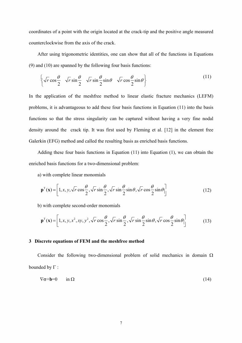
After using trigonometric identities, one can show that all of the functions in Equations

(9) and (10) are spanned by the following four basis functions:

cos sin sin sin cos sin

2 2 2 2r r r rθ θ θ θθ θ

(11)

In the application of the meshfree method to linear elastic fracture mechanics (LEFM)

problems, it is advantageous to add these four basis functions in Equation (11) into the basis

functions so that the stress singularity can be captured without having a very fine nodal

density around the crack tip. It was first used by Fleming et al. [12] in the element free

Galerkin (EFG) method and called the resulting basis as enriched basis functions.

Adding these four basis functions in Equation (11) into Equation (1), we can obtain the

enriched basis functions for a two-dimensional problem:

a) with complete linear monomials

T ( ) 1, , , cos , sin , sin sin , cos sin2 2 2 2

x y r r r rθ θ θ θθ θ = p x (12)

b) with complete second-order monomials

T 2 2( ) 1, , , , , , cos , sin , sin sin , cos sin2 2 2 2

x y x xy y r r r rθ θ θ θθ θ = p x (13)

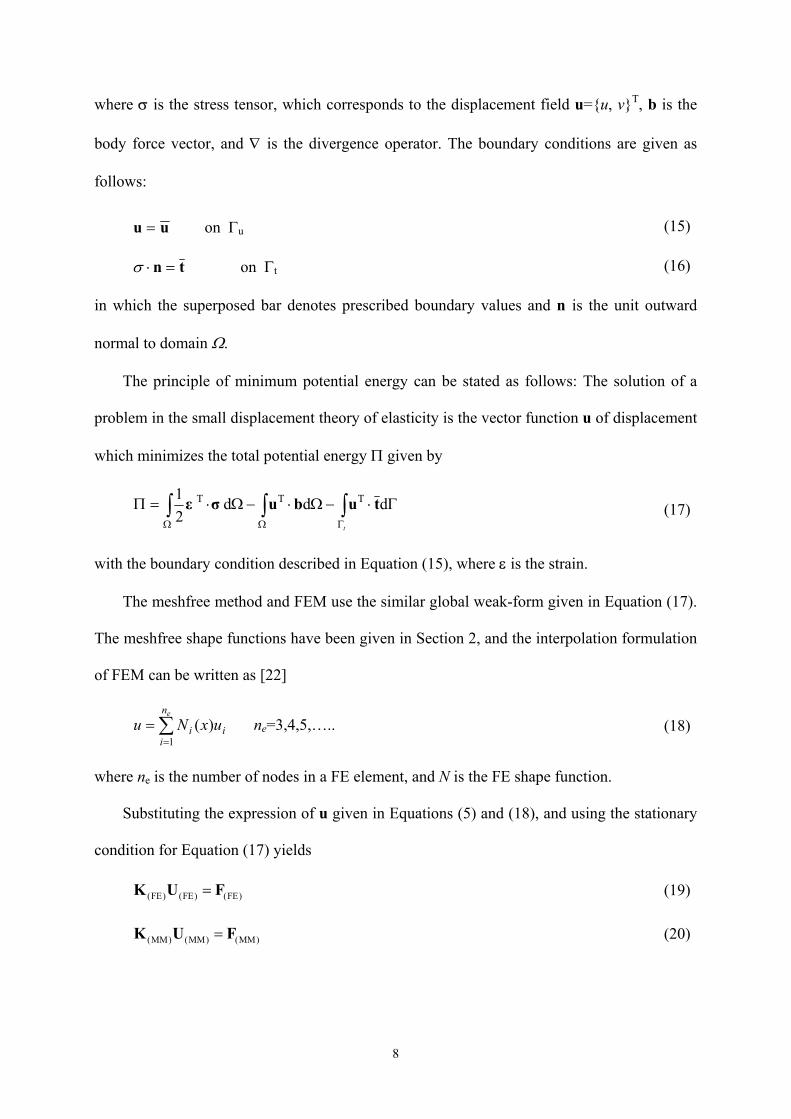
3 Discrete equations of FEM and the meshfree method

Consider the following two-dimensional problem of solid mechanics in domain Ω

bounded by Γ :

∇σ+b=0 in Ω (14)

8

where σ is the stress tensor, which corresponds to the displacement field u=u, vT, b is the

body force vector, and ∇ is the divergence operator. The boundary conditions are given as

follows:

uu = on Γu (15)

tn =⋅σ on Γt (16)

in which the superposed bar denotes prescribed boundary values and n is the unit outward

normal to domain Ω.

The principle of minimum potential energy can be stated as follows: The solution of a

problem in the small displacement theory of elasticity is the vector function u of displacement

which minimizes the total potential energy Π given by

∫ ∫ ∫Ω Ω Γ

Γ⋅−Ω⋅−Ω⋅=Πt

ddd21 TTT tubuσε (17)

with the boundary condition described in Equation (15), where ε is the strain.

The meshfree method and FEM use the similar global weak-form given in Equation (17).

The meshfree shape functions have been given in Section 2, and the interpolation formulation

of FEM can be written as [22]

∑=

=en

iii uxNu

1)( ne=3,4,5,….. (18)

where ne is the number of nodes in a FE element, and N is the FE shape function.

Substituting the expression of u given in Equations (5) and (18), and using the stationary

condition for Equation (17) yields

(FE) (FE) (FE)=K U F (19)

(MM) (MM) (MM)=K U F (20)

9

where (FE)K , (FE)U , (FE)F , (MM)K , (MM)U , and (MM)F are stiffness matrices, the displacement

vectors, and the force vectors for FEM and the meshfree method. Now, we have

T

(FE) (FE) (FE) dij i jΩ

= Ω∫K B DB (21)

T

(MM) (MM) (MM) dij i jΩ

= Ω∫K B DB (22)

t

(FE) d di i iN NΓ Ω

= Γ + Ω∫ ∫F t b (23)

t

(MM) d di i iφ φΓ Ω

= Γ + Ω∫ ∫F t b (24)

where D is the matrix of material constants, and

,

(FE) ,

, ,

00i x

i i y

i y i x

NN

N N

=

B , ,

(MM) ,

, ,

00i x

i i y

i y i x

φφ

φ φ

=

B (25)

4 Coupling of the meshfree method and FEM

4.1 Transition condition

As shown in Figure 2, consider a two-dimensional problem domain with a crack. A sub-

domain, Ω(MM), including the crack is discretized by the meshfree nodes and the other sub-

domain, Ω(FE), uses FEM. These two domains are joined by a transition domain Ω(T) that

possesses displacement compatibility and force equilibrium in coupling Ω(MM) and Ω(FEM).

This means that

(MM) (FE)k k=u u (26)

(MM) (FE) 0k k+ =f f (27)

where (MM)ku , (FE)ku , (MM)kf and (FE)kf are displacements and forces at a transition particle k

obtained by the meshfree method in Ω(MM) and FEM in Ω(FE), respectively.

10

It will be ideal to satisfy both the displacement compatibility and the force equilibrium

conditions, in which the displacement compatibility Equation (26) is the most important and

must be satisfied. In addition, because the meshfree MLSA shape functions lack the delta

function properties, it is difficult to directly connect these two domains.

To satisfy the displacement compatibility condition, two combination techniques, using

the hybrid displacement shape function algorithm [16] and the modified variational form

algorithm [17], have been developed. However, in these techniques, as shown in Figure 1, a

common interface (a curve in the two-dimensional problem) is used between Ω(FE) and Ω(MM).

The meshfree nodes and the FEM nodes along this interface coincide with each other, and are

dependent on each other. It will increase the computational cost and make difficulty for some

problems. In addition, because only an interface curve is used, it is difficult to ensure the

compatibility (especially the high-order continuity). In the following, we will develop a new

transition technique to ensure a smooth transition between Ω(FE) and Ω(MM), which has been

successfully used in the macro/micro/nano multiscale analysis [23].

4.2 Coupling technique

As shown in Figure 2, there is a transition (or bridge) region, Ω(T), between the FEM and

meshfree domains. The generalized displacement of a point in the transition domain at x can

be defined as

(MM) ( )( ) ( )= − FEg u x u x (28)

where (MM) ( )ku x and (FE) ( )ku x are the displacements of a point x, obtained by the

interpolations using the meshfree nodes and the FEM element, respectively, i.e.,

(MM) (MM)( ) ( )k I k II

=∑u x Φ x u (29)

(FE) (FE)( ) ( )k J k JJ

=∑u x N x u

(30)

11

A sub-functional is introduced to enforce the displacement compatibility condition given

in Equation (26) by means of Lagrange multiplier λ in the transition domain

(T ) (T )

(T ) (T )

(T) (MM) (FE)

(MM) (FE)

(MM) (FE)(T) (T)

d d

d d

Ω Ω

Ω Ω

Π = ⋅ Ω = ⋅ − Ω

= ⋅ Ω− ⋅ Ω

= Π −Π

∫ ∫

∫ ∫

λ g λ u u

λ u λ u (31)

In which, (MM)(T)Π and (FE)

(T)Π are the sub-functional for the meshfree part and the FEM part.

Substituting (MM)(T)Π and (FE)

(T)Π separately into Equation (17) for the meshfree method and

FEM, generalized functional forms can be written as

( MM ) ( MM ) (T )( MM )

T T T(MM) (MM)

1 d d d d2

tΩ Ω Γ Ω

Π = ⋅ Ω− ⋅ Ω− ⋅ Γ + ⋅ Ω∫ ∫ ∫ ∫ε σ u b u t λ u (32)

( FE ) ( FE ) (T )( FE )

T T T(FE) (FE)

1 d d d d2

tΩ Ω Γ Ω

Π = ⋅ Ω − ⋅ Ω− ⋅ Γ − ⋅ Ω∫ ∫ ∫ ∫ε σ u b u t λ u (33)

In these variational formulations, the domains of Ω(FE) and Ω(MM) are connected via Lagrange

multiplier λ, which can be given by the interpolation functions Λ and the nodal value of λi

i ii

= Λ ⋅∑λ λ (34)

Λ is the selected interpolation for λi and it can be the FEM shape function.

Substituting Equations (5) and (34) into Equation (32), and using the stationary condition

based on the displacement, the following meshfree equations can be obtained

(MM)(MM) (MM) (MM)

=

UK B F

λ (35)

where (MM)K and (MM)F have been defined in Equations (22) and (24), (MM)B is defined as

(T )

T(MM) d

Ω

= Ω∫B ΛΦ (36)

12

Substituting Equations (18) and (34) into Equation (33), and using the stationary

condition based on the displacement, lead to the following FEM equations

(FE)(FE) (FE) (FE)

− =

UK B F

λ (37)

where (FE)K and (FE)F have been defined in Equations (21) and (23), (FE)B is defined as

(T )

T(FE) d

Ω

= Ω∫B ΛN (38)

It should be mentioned here that it is impossible to solve Equations (35) and (37)

separately. To obtain the unique solution for the global problem, Using the stationary

condition of Equations (35) and (37) based on the of Lagrange multiplier and considering the

compatibility condition,, we can obtain the following relationship,

(MM) (MM) (FE) (FE)T T− =B U B U 0 (39)

Because the meshfree and FEM domains are connected through the transition domain, the

assembly of Equations (35), (37) and (39) yields a linear system of the following form

(MM) (MM) (MM) (MM)

(FE) (FE) ( ) (FE)

(MM) (FE)T T

− =

−

FE

K 0 B U F0 K B U F

B B 0 λ 0 (40)

Solving Equation (40) together with the displacement boundary condition, given in Equation

(15) , we can obtain the solution for the problem considered.

To satisfy the force equilibrium condition, the generalized derivative at a point x can be

written as

(MM) (FE)( )

( ) ( )x

∂ ∂= −

∂ ∂

u x u xg

x x (41)

Using Lagrange multiplier γ , we have

13

(T )

(T ) (T )

(T)( )

(MM) (FE)

(MM) (FE)(T)( ) (T)( )

d

( ) ( )d d

Ω

Ω Ω

Π = ⋅ Ω

∂ ∂= ⋅ Ω− ⋅ Ω

∂ ∂

= Π −Π

∫

∫ ∫

x

x x

γ g

u x u xγ γ

x x (42)

Following the similar procedure from Equation (32) to Equation (40), we can obtain the

coupling equations to satisfy the high-order continuity

(MM) (MM) (MM) (MM) (MM)

(FE) (FE) (FE) ( ) (FE)

(MM) (FE)

(MM) (FE)

T T

T T

− − = − −

FE

K 0 B A U F0 K B A U FB B 0 0 λ 0A A 0 0 γ 0

(43)

where

(T )

T

(MM) dΩ

∂= Ψ Ω

∂∫ΦAx

, (44)

(T )

T

(FE) dΩ

∂= Ψ Ω

∂∫NAx

(45)

In which Ψ is the interpolation functions for γ.

4.3 Numerical implementations

a) The size of transition region

The size of transition region will affect the performance of the coupled method. If the size

is too small, it will decrease the accuracy of the transition, especially for the high order

compatibility. If the size is too big, it will significantly increase the computational cost. For

many problems, it is reasonable to use the following size of transition region:

FE(3 ~ 5)th d≅ ⋅ or MM(3 ~ 5) d⋅ (46)

where dFE and dMM are equivalent sizes of FEM element and meshfree nodal space.

b) The transition particles

14

To get B(MM) and B(FEM) numerically, the transition region can be divided into regular

background cells, which are similar of those used in the meshfree method. However, these

cells are totally independent of the FE elements and the meshfree background cells. In the

practical computation, to simplify the integration and reduce the “meshing” cost, several

layers of transition particles, which are regularly distributed, can be inserted in the transition

domain Ω(T). The displacement compatibility between FEM and meshfree nodes is achieved

through these transition particles.

The advantages of using these transition particles are clear. First, they allow the meshfree

nodes in Ω(MM) to have an arbitrary distribution and become independent of the distributions

of the FEM nodes in Ω(FE). Second, the compatibility conditions in the transition domain can

be conveniently controlled through the adjustment of the number and distribution of the

transition particles. For some sub-transition domains with stronger compatibility requirement,

a finer transition particle distribution can be arranged. Third, the compatibility of higher order

derivatives can be easily satisfied.

c) Lagrange multipliers

The above Lagrange multiplier method is accurate and the physical meaning is also very

clear. However, it will increase the computational cost (especially when the number of

transition particles is large) because new variables (Lagrange multipliers) are added. Hence,

we can use the constant Lagrange multipliers to yield the so-called penalty method, i.e., the

common Lagrange multiplier method can be used to obtain a range of penalty coefficients,

and then use them as constants for this problem and other similar problems to improve

computational efficiency.

15

5 The relay model

With the use of node based interpolation techniques, meshfree methods offer great

opportunities to handle problems of complex geometry including cracks. However, there is

general discontinuity of displacements across a crack, and the interpolation domain used for

the construction of meshfree shape functions can contain numerous irregular boundary

fragments and the computation of nodal weights based on physical distance can be erroneous.

This issue will become more serious in dealing with the fracture problems, especially for the

multi-cracking problems. Several techniques have been reported on the construction of

meshfree approximations with discontinuities and non-convex boundaries, including the

visibility method [2], the diffraction method [24], and the transparency method [24].

However, these methods are only effective for problems with relatively simple domains (e.g.

with one or two cracks, or not many non-convex portions on the boundaries), but not effective

for domains with highly irregular boundaries (e.g., with many cracks). Liu and Tu [25] have

developed a relay model to determine the domain of influence of a node in a complex

problem domain.

The relay model is motivated by the way of a radio communication system composed of

networks of relay stations. Consider an interpolation domain containing a large number of

irregular boundary fragments (or cracks) as shown in Figure 3, in which O is the interpolation

point, P is the field node, and R is the relay point. The field node, e.g., P2, first radiates its

influence in all directions equally, liking a radio signal being broadcasted at a radio station,

until the contained boundaries are encountered. Then its’ influence is relayed through relay

points, e.g., R2-1 and R1-1, to reach the interpolation point O. The distance (called equivalent

distance) between the interpolation point and the field node can then be calculated. In

addition, the weight parameter used in MLSA is measured by the equivalent distance that can

16

be computed based on the relay region defined by a circle involute. The details for the relay

model can be find in Liu [20] and Liu and Tu [25].

6 Numerical results and discussions

Several cases of two-dimensional fracture problems have been studied in order to examine

the present coupled MM/FE method. Except when mentioned, the units are taken as standard

international (SI) units in the following examples.

6.1 Cantilever beam

The coupled method is first verified by a two-dimensional cantilever beam problem,

because its’ analytical solution is available and can be found in textbooks e.g., Timoshenko

and Goodier[26]. Consider a beam, as shown in Figure 4(a), with length L and height D

subjected to a parabolic traction at the free end. The parameters of the beam are taken as

E=3.0×107, ν=0.3, D=12, L=48, and P=1000. The beam has a unit thickness and a plane stress

problem is considered.

As shown in Figure 4(b), the beam is divided into two parts. FEM using the triangular

elements is used in the left part where the essential boundary condition is included. The

meshfree method is used in the right part where the traction boundary condition is included.

These two parts are connected through a transition region that is discretized by 54 regularly

distributed transition particles. Figure 5 illustrates the comparison between the shear stress

calculated analytically and by the coupled method at the cross-section of x=L/2, which shows

an excellent agreement between the analytical and numerical results.

17

6.2 Near-tip crack field

A well-known near-tip field, which is subjected to mode-I displacement field at its edges,

is analyzed. As shown in Figure 6, an edge-cracked square plate is subjected to the following

displacement field for a model-I crack [1].

2

2

cos 1 2sin2 2

2 2sin 1 2cos

2 2

Iu K rv

θ θκ

µ π θ θκ

− + = + −

(47)

Hence, the analytical solution for the stress field is given in Equation (9).

The plate is divided into two parts: the meshfree method is used for the central part, in

which the crack embedded, and FEM is used for other parts. The computational model is

plotted in Figure 7: 441 irregularly distributed nodes are used in the meshfree domain, 578

triangular FEM elements are used in the FEM domain, and 210 regularly distributed transition

particles are used in the transition domains. Figure 8 shows the stress distribution along the

crack axis (when θ=0°). Clearly, the prediction of the new developed method matches the

analytical solution very well.

It should be mentioned that the sole FEM will lead to worse accuracy for this problem,

especially for the stress distributions around the crack tip, because FEM without the enriched

basis function usually has bad accuracy and is difficult to capture the stress singularity near

the crack tip. Although using the high-order FEM elements can partly solve this issue, FEM

still has technical difficulty for the fracture problems (especially the dynamic fracture

problems). It has also been proven [12] that the sole meshfree method has much better

accuracy for the crack problem. However, the computational efficiency will be worse if the

sole meshfree method is used. Our studies show that the present coupled method can keep the

good accuracy of the meshfree method for the crack tip field, and, at the same time, it can

18

save much computational cost because of the use of FEM in the regions far away from the

crack tip.

6.3 Two edge-cracked plates loaded in tension

An edge-cracked square plate subjected to a uniformed tension of 1.0f = , as shown in

Figure 9, is studied. The plane strain case is considered, and 1000, 0.25E ν= = . The

analytical results for KI had been given by Gdoutos [28] and Ching and Batra [27]. For these

parameters used here, the analytical ( ) 11.2I analyticalK = .

The computational model is the same as that used in Section 6.2 and shown in Figure 7.

Stress intensity factors were computed using the domain form of the J-integral. Our study

found that the coupled method using the MLSA with the enriched basis functions makes the

J-integral almost domain independent, given to ( ) 11.31I numericalK = . Compared with the

analytical solution, the coupled method leads to a stable and accurate result.

A square plate with double edge-cracks shown in Figure 10 is also studied. The

computational model in Figure 11 contains 705 irregularly distributed nodes in the meshfree

domain, 538 triangular FEM elements in the FEM domain, and 210 regularly distributed

transition particles in the transition domains. Ching and Batra [27] studied the same problem

and the analytical KI given by Gdouos [28] is ( ) 4.65I analyticalK = . Using the J-integral, the

present coupled method gives ( ) 4.75I numericalK = . The coupled method leads to a very

accurate result.

6.4 Shear edge crack

In this example, a clamped plate with an edged crack and subjected to shear traction is

considered. The parameters have been shown in Figure 12. The material constants used are

63.0 10E = × units and 0.25υ = . A plane strain state of deformation is assumed. The

19

reference solution for the stress intensity factors has been given by Fleming et al. ([12] and

Ching and Batra [27] with 34IK = and 4.55IIK = . Our computational model in Figure 13

has 284 irregularly distributed nodes in the meshfree domain, 280 bi-linear FEM elements in

the FEM domain, and 180 regularly distributed transition particles in the transition domains.

The present coupled method works well for this problem and the computational errors are less

than 2% for both KI and KII.

6.5 Cracks in a complex shaped plate

Let us now consider a plate of complex shape with a “C” shaped crack. The material

constants used are 73.0 10E = × and 0.3υ = . One edge of the plate is fixed, one edge is

subjected to uniformly distributed tension load, and the rest are traction free. As shown in

Figure 14, the plate is divided into two parts. The meshfree method is used in the central part

including the crack, and FEM is used for other parts. The computational model shown in

Figure 15 contains 595 irregularly distributed nodes in the meshfree domain, 660 triangular

FEM elements in the FEM domain, and 560 regularly distributed transition particles in the

transition domains. As a reference solution, this problem is also analyzed by the sole meshfree

method (the software of MFree 2D: Liu [20]) with very fine nodal distribution. Figure 16

shows the distribution of stress, σxx. It is almost identical with the meshfree method result.

Table 1 lists the comparison of displacements and stress of four points shown in Figure 14.

Figure 17 shows the stress distribution along y-axis, and, again, very good agreement is

obtained between the coupled method and the purely meshfree method. The stress

concentrations on the crack tips have been clearly shown with the stress concentration factor

around 3.3.

It should be mentioned here that for this problem the coupled method uses less

computational cost than the pure meshfree method, because we only apply the meshfree

20

method in a very small region (about 10% of the problem domain) and FEM is used in other

area when FEM has a better computational efficiency than the meshfree method (Liu and Gu

[13] ). Hence, the advantage of the present coupled method has been proven by this example.

Table 1 The displacements and stresses for four points in this plate

Displacement Stress

u( 710−× ) v ( 710−× ) xxσ yyσ xyτ

MFree 2D 4.1 3.4 2.31 -0.02 -0.03 Point A

The coupled method 3.9 3.2 2.27 -0.017 -0.028

MFree 2D 4.9 2.8 -0.57 -1.6 -0.45 Point B

The coupled method 4.7 2.9 -0.61 -1.72 -0.55

MFree 2D 5.3 4.2 -0.56 -1.05 0.36 Point C

The coupled method 5.2 4.0 -0.54 -1.01 0.32

MFree 2D 4.5 4.3 3.51 1.13 1.37 Point D

The coupled method 4.2 4.2 3.34 1.08 1.32

7 Concluding remarks

FEM often has experiences difficulties in fracture mechanics problems because of

difficulty in the re-meshing. Meshfree methods are effective for these crack problems, but

they usually have worse computational efficiency. In the analysis of crack problems, we can

find that a crack region usually occupies only a small part in the whole problem domain. It is

desirable and beneficial to combine the meshfree methods with FEM in order to exploit their

advantages while evading their disadvantages.

A novel coupled meshfree/FEM method has been developed in this paper for the analysis

of crack problems. In this coupled method, the meshfree method is used only in a sub-domain

including the crack and FEM is employed in the remaining part. Several numerical techniques

are developed to ensure the effectiveness for this coupled method, including:

21

a) The transition particles are inserted in the transition domain. Through these particles, a

Lagrange multiplier method is used to ensure the compatibility of displacements and their

gradients in the transition.

b) The relay model is used for the effective construction of meshfree interpolation

domains considering the discontinuous boundaries.

Numerical examples have been studied to demonstrate effectiveness of the present

coupled method for crack problems, and very goods results have been obtained. The coupled

method holds the advantages of both the FEM and meshfree methods including: 1) a lower

computation cost; 2) a good accuracy; 3) the enhanced compatibility in the transition domain

between the FEM domain and meshfree domain. Hence, it has been proven that the new

coupled method is effective and robust for the analysis of fracture mechanics problems, and it

has very good potential to become a powerful numerical tool.

Acknowledgement

This work was supported by an ARC Discovery Grant.

References

[1] Gingold RA and Moraghan JJ (1977), Smooth particle hydrodynamics: theory and

applications to non spherical stars. Monthly Notices of the Royal Astronomical Society,

181, 375-389.

[2] Belytschko T, Lu YY and Gu L (1994), Element-Free Galerkin Methods. International

Journal for Numerical Methods in Engineering, 37:229-256.

[3] Liu WK, Jun S, Zhang Y (1995), Reproducing kernel particle methods. International

Journal for Numerical Methods in Engineering, 20: 1081-1106.

[4] Liew KM, Wu YC, Zou GP, Ng TY (2002). Elasto-plasticity revisited: numerical analysis

via reproducing kernel particle method and parametric quadratic programming. Int. J.

Numer. Meth. Engng, 55:669–683.

22

[5] Atluri SN and Shen SP (2002), The Meshfree Local Petrov-Galerkin (MLPG) method.

Tech Sciemce Press. Encino USA.

[6] Atluri SN and Zhu T (1998), A new meshfree local Petrov-Galerkin (MLPG) approach in

computational mechanics. Computational Mechanics, 22: 117-127.

[7] Gu YT and Liu GR (2001a), A meshfree local Petrov-Galerkin (MLPG) method for free

and forced vibration analyses for solids, Computational Mechanics, 27 (3): 188-198.

[8] Gu YT and Liu GR (2001b), A local point interpolation method for static and dynamic

analysis of thin beams, Computer Methods in Applied Mechanics and Engineering, 190:

5515-5528.

[9] Liu GR and Gu YT (2001b), A local radial point interpolation method (LR-PIM) for free

vibration analyses of 2-D solids. Journal of Sound and Vibration, 246(1): 29-46.

[10] Wang QX, Lam KY, et al. (2003). Analysis of microelectromechanical systems (MEMS)

by meshless Local Kriging (LoKriging) method. Journal of Chinese Institute of

Engineers; 27 (4): 573-583.

[11] Liew KM and Chen XL (2004), Mesh-free radial point interpolation method for the

buckling analysis of Mindlin plates subjected to in-plane point loads, International

Journal for Numerical Methods in Engineering, 60(11): 1861-1877.

[12] Fleming, M.; Chu, Y.; Moran, B.; Belytschko, T.(1997): Enriched element-free Galerkin

methods for crack tip fields. International Journal for Numerical Methods in

Engineering, 40: 1483-1504.

[13] Liu GR and Gu YT (2005), An introduction to meshfree methods and their

programming. Springer Press, Berlin.

[14] Belytschko T, Organ D (1995) Coupled finite element-element–free Galerkin method.

Computational Mechanics, 17:186-195

[15] Hegen D (1996), Element-free Galerkin methods in combination with finite element

approaches. Comput. Methods Appl. Mech. Engrg., 135: 143-166.

[16] Gu YT and Liu GR(2001c), A coupled element free Galerkin/Boundary element method

for stress analysis of two-dimensional solids, Computer Methods in Applied Mechanics

and Engineering, 190/34: 4405-4419.

23

[17] Gu YT and Liu GR(2003), Hybrid boundary point interpolation methods and their

coupling with the element free Galerkin method. Engineering Analysis with Boundary

Elements, 27(9): 905-917.

[18] Liu GR and Gu YT(2000), Meshfree Local Petrov-Galerkin (MLPG) method in

combination with finite element and boundary element approaches. Computational

Mechanics, 26(6): 536-546.

[19] Gu YT and Liu GR (2005), Meshfree methods coupled with other methods for solids and

structures. Tsinghua Science and Technology, 10 (1): 8-15.

[20] Liu GR (2002), Mesh Free Methods: Moving Beyond the Finite Element Method. CRC

press, USA

[21] Anderson, T. L. (1991): Fracture Mechanics: Fundamental and Applications (1st Ed.)

CRC Press.

[22] Zienkiewicz OC and Taylor RL (2000), The Finite Element Method. 5th edition,

Butterworth Heinemann, Oxford, UK.

[23] Gu YT and Zhang LC (2006), A concurrent multiscale method for structures based on

the combination of the meshfree method and the molecular dynamics. Multiscale

Modeling and Simulation: A SIAM Interdisciplinary Journal, 5 (4): 1128-1155.

[24] Organ DJ, Fleming M, Belytschko T (1996):Continuous meshfree approximations for

nonconvex bodies by diffraction and transparency. Computational Mechanics, 18: 225-

235.

[25] Liu GR and Tu, ZH(2002), An Adaptive Procedure Based on Background Cells for

Meshfree Methods, Comput. Methods in Appl. Mech. and Engrg., 191: 1923-1943.

[26] Timoshenko SP and Goodier JN (1970), Theory of Elasticity, 3rd Edition. McGraw-hill,

New York.

[27] Ching HK and Batra RC (2001), Determination of Crack Tip Fields in Linear

Elastostatics by the Meshfree Local Petrov-Galerkin (MLPG)Method. CMES, 2(2):

273-289

[28] Gdoutos, E. E. (1993): Fracture Mechanics: an Introduction. Kluwer Academic

Publishers.

24

Figure Caption:

Figure 1 The coupled techniques using the interface boundary

Figure 2 The coupled analysis for the crack problem using the new transition technique

Figure 3 Relay model for an irregular domain with discontinuous boundaries

Figure 4(a) A cantilever beam subjected to a parabolic traction at the free end

Figure 4(b) The computational model for the two-dimensional cantilever beam

Figure 5 Shear stress distributions on the cross-section of the beam at x=L/2

Figure 6 A cracked square plate subjected to Mode-I displacement boundary conditions

Figure 7 The computational model for the edge cracked plate

Figure 8 The distribution of σyy along the axis of the crack (θ=0)

Figure 9 An edge square plate subjected to the tension loading

Figure 10 A double-edge square plate subjected to the tension loading

Figure 11 The computational model for the plate with two edge cracks

Figure 12 An edge-cracked plate subjected to the shear loading

Figure 13 The computational model for the edge-cracked plate subjected to the shear loading

Figure 14 A plate with a “C” shaped center crack

Figure 15 The computational model for the plate with the “C” shaped center crack

Figure 16 The distribution of σxx

Figure 17 The distribution of σxx and σyy along the y axis