Gu, Xu (2010) Systems biology approaches to the computational
311
Systems Biology Approaches to the Computational Modelling of Trypanothione Metabolism in Trypanosoma brucei by Xu Gu A dissertation submitted to The Department of Computing Science of The University of Glasgow for the degree of Doctor of Philosophy March 2010 c Xu Gu, 2010.
Transcript of Gu, Xu (2010) Systems biology approaches to the computational


Systems Biology Approaches to theComputational Modelling of Trypanothione
Metabolism in Trypanosoma brucei
by
Xu Gu
A dissertation submitted to
The Department of Computing Science
ofThe University of Glasgow
for the degree of
Doctor of Philosophy
March 2010
c©Xu Gu, 2010.

2
Abstract
This work presents an advanced modelling procedure, which applies both struc-tural modelling and kinetic modelling approaches to the trypanothione metabolicnetwork in the bloodstream form of Trypanosoma brucei, the parasite responsiblefor African Sleeping sickness. Trypanothione has previously been identified asan essential compound for parasitic protozoa, however the underlying metabolicprocesses are poorly understood. Structural modelling allows the study of thenetwork metabolism in the absence of sufficient quantitative information of tar-get enzymes. Using this approach we examine the essential features associatedwith the control and regulation of intracellular trypanothione level. The firstdetailed kinetic model of the trypanothione metabolic network is developed,based on a critical review of the relevant scientific papers. Kinetic modellingof the network focuses on understanding the effect of anti-trypanosomal drugDFMO and examining other enzymes as potential targets for anti-trypanosomalchemotherapy.
We also consider the inverse problem of parameter estimation when the sys-tem is defined with non-linear differential equations. The performance of arecently developed population-based PSwarm algorithm that has not yet beenwidely applied to biological problems is investigated and the problem of param-eter estimation under conditions such as experimental noise and lack of infor-mation content is illustrated using the ERK signalling pathway. We proposea novel multi-objective optimization algorithm (MoPSwarm) for the validationof perturbation-based models of biological systems, and perform a comparativestudy to determine the factors crucial to the performance of the algorithm. By si-multaneously taking several, possibly conflicting aspects into account, the prob-lem of parameter estimation arising from non-informative experimental measure-ments can be successfully overcome. The reliability and efficiency of MoPSwarmis also tested using the ERK signalling pathway and demonstrated in model val-idation of the polyamine biosynthetic pathway of the trypanothione network.
It is frequently a problem that models of biological systems are based on arelatively small amount of experimental information and that extensive in vivoobservations are rarely available. To address this problem, we propose a newand generic methodological framework guided by the principles of Systems Bi-ology. The proposed methodology integrates concepts from mathematical mod-elling and system identification to enable physical insights about the system tobe accounted for in the modelling procedure. The framework takes advantageof module-based representation and employs PSwarm and our proposed multi-objective optimization algorithm as the core of this framework. The methodolog-ical framework is employed in the study of the trypanothione metabolic network,specifically, the validation of the model of the polyamine biosynthetic pathway.Good agreements with several existing data sets are obtained and new predic-tions about enzyme kinetics and regulatory mechanisms are generated, whichcould be tested by in vivo approaches.

3
Acknowledgements
This thesis would not have been possible without the help and support of
many people.
I am indebted to Professor Ray Welland for the financial support provided
by the Department of Computing Science during the third year of my research
and the writing-up period, without which I could not have completed my study
at Glasgow. I would also like thank him for his interest in my work.
I would like to thank Professor David Gilbert for his guidance, help and
encouragement throughout my research programme. Without his belief and
interest in my work, this thesis would not have been possible.
I would like to thank Professor Des Higham (Department of Mathematics,
University of Strathclyde) for his knowledge, direction and perceptiveness. His
noteworthy comments and constructive criticism on my work have been invalu-
able. I have benefited from his fascinating ideas on the research subject at every
visit to the Strathclyde University.
I would like to thank Professor Mike Barrett for his motivation and advice
throughout the thesis. Many thanks to him for bringing me into this fantastic
research domain concerning African Sleeping sickness. Thanks also go to the
members in his research group at Glasgow Biomedical Research Center for their
interest in my work, particularly, Isabel Vincent for her work on arginase.
I am very grateful to Professor Rainer Breitling, Dr. Barbara Bakker (The
University of Groningen) and Professor Margaret Philips (The University of
Texas Southwestern Medical Center) for their advice, experimental data and
hours of conversation.
Finally I would like to thank my parents for their understanding, endless
patience and constant support.
And of course, Dave, for always being there for me.

4
Declaration
This thesis has not been previously been accepted in substance for any degree
and is not being concurrently submitted in candidature for any degree
All the work reported in this thesis has been performed by myself, except
where otherwise stated. Other sources are acknowledged explicitly in the text.
A bibliography is appended.
Xu Gu
March 2010.

Contents
1 Introduction 15
1.1 Scope of the Thesis . . . . . . . . . . . . . . . . . . . . . . . . . . 15
1.2 Systems Biology . . . . . . . . . . . . . . . . . . . . . . . . . . . . 16
1.3 Computational Modeling . . . . . . . . . . . . . . . . . . . . . . . 17
1.4 Metabolic Modelling . . . . . . . . . . . . . . . . . . . . . . . . . 21
1.5 System Identification . . . . . . . . . . . . . . . . . . . . . . . . . 22
1.6 Trypanothione Metabolic Pathway . . . . . . . . . . . . . . . . . 23
1.7 Thesis Statement . . . . . . . . . . . . . . . . . . . . . . . . . . . 25
1.8 Thesis Contributions . . . . . . . . . . . . . . . . . . . . . . . . . 26
1.9 Outline of the Dissertation . . . . . . . . . . . . . . . . . . . . . . 27
1.10 Publications . . . . . . . . . . . . . . . . . . . . . . . . . . . . . . 29
2 Background and Related Work 30
2.1 Biological Systems . . . . . . . . . . . . . . . . . . . . . . . . . . 30
2.1.1 Metabolic Pathway . . . . . . . . . . . . . . . . . . . . . . 31
2.1.2 Gene Regulatory Pathway . . . . . . . . . . . . . . . . . . 31
2.2 Metabolic Network and Regulation . . . . . . . . . . . . . . . . . 33
2.3 Mathematical Modelling Formalism . . . . . . . . . . . . . . . . . 38
2.3.1 Ordinary Differential Equations . . . . . . . . . . . . . . . 40
2.3.2 Stochastic Master Equations . . . . . . . . . . . . . . . . . 41
2.3.3 Computational Simulation . . . . . . . . . . . . . . . . . . 42
2.4 System Identification . . . . . . . . . . . . . . . . . . . . . . . . . 44
2.5 Network Modularity . . . . . . . . . . . . . . . . . . . . . . . . . 48
2.6 Discussion . . . . . . . . . . . . . . . . . . . . . . . . . . . . . . . 50
3 Structural Modelling 52
3.1 Overview . . . . . . . . . . . . . . . . . . . . . . . . . . . . . . . . 52
3.2 Biological Background . . . . . . . . . . . . . . . . . . . . . . . . 53
5

LIST OF FIGURES 11
7.3 The first three stages of model decomposition of the trypanothione
biosynthesis sub-system . . . . . . . . . . . . . . . . . . . . . . . 213
7.4 Simulation profiles of the key metabolites compared to experi-
mental data in Stage 2 . . . . . . . . . . . . . . . . . . . . . . . . 214
7.5 Simulation profiles for the arginine dynamics obtained in Stage 2
of the model decomposition . . . . . . . . . . . . . . . . . . . . . 215
7.6 Simulation profiles of the key metabolites compared to experi-
mental data in Stage 3 . . . . . . . . . . . . . . . . . . . . . . . . 217
7.7 Results of decompositional Stage 3, arginine-centered strategy . . 218
7.8 Simulation profiles of the arginine and ornithine dynamics with
the modified arginase kinetics . . . . . . . . . . . . . . . . . . . . 221
7.9 Simulation profiles of the arginine and ornithine dynamics with
the modified kinetics of arginase and arginine transporter . . . . . 222
7.10 Simulation profiles of the key metabolites compared to observed
values when glutathione dynamics is approximated with different
experimental data . . . . . . . . . . . . . . . . . . . . . . . . . . . 226
7.11 Simulation profiles of spermidine and GspdSH compared to gene
knockdown data from Xiao et al. . . . . . . . . . . . . . . . . . . 228
7.12 Simulation profiles of trypanothione compared to gene knockdown
data from Xiao et al. . . . . . . . . . . . . . . . . . . . . . . . . . 229
7.13 The schematic representation of polyamine biosynthetic sub-pathway240
7.14 Simulation profiles of spermidine dynamics of polyamine biosyn-
thetic sub-pathway . . . . . . . . . . . . . . . . . . . . . . . . . . 241
7.15 Trade-off solutions of the polyamine model solved by MoPSwarm 243
7.16 Predicted concentration profiles of the steady-state model of the
polyamine biosynthetic sub-pathway . . . . . . . . . . . . . . . . 245
7.17 Predicted concentration profile of the perturbed model of the
polyamine biosynthetic sub-pathway . . . . . . . . . . . . . . . . 247
7.18 Effects of ODC knockdown on polyamine levels in time-dependent
model simulations . . . . . . . . . . . . . . . . . . . . . . . . . . . 248
7.19 Effects on polyamine levels in time-dependent simulations induced
by AdoMetDC knockdown . . . . . . . . . . . . . . . . . . . . . . 249
7.20 Effects on polyamine levels in time-dependent simulations induced
by prozyme knockout . . . . . . . . . . . . . . . . . . . . . . . . . 250
7.21 Effects of changes in parameter β on polyamine levels computed
at the end of simulation . . . . . . . . . . . . . . . . . . . . . . . 251

LIST OF FIGURES 12
7.22 Effects of a three-fold AHS activity up-regulation on polyamine
levels in time-dependent model simulations . . . . . . . . . . . . . 252
7.23 Effects of changes in AHS enzyme related apparent coefficient on
the concentration levels of AdoMet and dAdoMet computed at
the end of simulation . . . . . . . . . . . . . . . . . . . . . . . . . 253

List of Tables
1.1 Data on human African trypanosomiasis (Barrett et al. 2003). . . 24
3.1 Reaction names and stoichiometries of the model shown in Fig-
ure 3.2. . . . . . . . . . . . . . . . . . . . . . . . . . . . . . . . . . 61
3.2 Enzyme subsets of the trypanothione pathway. . . . . . . . . . . . 65
3.3 Elementary modes of the trypanothione model shown in Figure 3.2. 66
3.4 Elementary modes of the identified structural topologies of the
trypanothione pathway summarized in Figure 3.3. . . . . . . . . . 69
3.5 Enzyme subsets of the trypanothione pathway depicted in ST1. . 79
3.6 Steady-state flux distribution predicted by LP optimization . . . . 84
4.1 Parameter values for T. brucei ODC. . . . . . . . . . . . . . . . . 106
4.2 Parameter values for T. brucei AdoMetDC. . . . . . . . . . . . . 111
4.3 Parameter values for T. brucei MAT. . . . . . . . . . . . . . . . . 112
4.4 Parameter values for L. donovani ARG. . . . . . . . . . . . . . . . 114
4.5 Parameter values for T. brucei SpdS. . . . . . . . . . . . . . . . . 116
4.6 Parameter values for the enzyme on the methionine recycling path
in T. brucei. . . . . . . . . . . . . . . . . . . . . . . . . . . . . . . 117
4.7 Parameter values for the enzyme of AdoHcy production in T. brucei.120
4.8 Parameter values for T. brucei γGCS. . . . . . . . . . . . . . . . . 123
4.9 Parameter values for T. brucei GS. . . . . . . . . . . . . . . . . . 123
4.10 Parameter values for T. brucei TryS and TryAdm. . . . . . . . . . 126
4.11 Parameter values for T. brucei TR . . . . . . . . . . . . . . . . . 129
4.12 Parameter values for T. brucei glucose transport. . . . . . . . . . 132
4.13 Parameter values for T. brucei HXK. . . . . . . . . . . . . . . . . 133
4.14 Parameter values for T. brucei G6PDH. . . . . . . . . . . . . . . 135
4.15 Parameter values for T. brucei 6PGDH. . . . . . . . . . . . . . . 136
4.16 The initial kinetic model of the trypanothione metabolism . . . . 137
13

LIST OF TABLES 14
4.17 Steady-state concentrations of the different metabolites and other
time-dependent variables of the trypanothione metabolism. . . . . 138
5.1 An ODE-based computational model of ERK signalling pathway. 155
5.2 Mean and standard deviation values of the parameters estimated
by PSwarm . . . . . . . . . . . . . . . . . . . . . . . . . . . . . . 162
5.3 Mean and standard deviation values of the parameters estimated
by PSwarmGM . . . . . . . . . . . . . . . . . . . . . . . . . . . . 162
6.1 The ODE-based computational model of ERK signalling pathway. 186
7.1 Differential equations for the different metabolites included in the
polyamine biosynthetic sub-pathway. . . . . . . . . . . . . . . . . 239
7.2 Estimated values of unknown parameters of the polyamine biosyn-
thetic sub-pathway. . . . . . . . . . . . . . . . . . . . . . . . . . . 244
7.3 Polyamine concentrations considered as the basal condition of the
polyamine model . . . . . . . . . . . . . . . . . . . . . . . . . . . 246
7.4 Comparison of the steady-state flux distributions in the polyamine
biosynthetic sub-pathway predicted via structural modelling and
kinetic modelling . . . . . . . . . . . . . . . . . . . . . . . . . . . 255
A.1 Dynamic responses of the intracellular metabolite concentrations
in bloodstream-form T. brucei . . . . . . . . . . . . . . . . . . . . 270
A.2 Dynamic responses of the intracellular metabolite concentrations
in procyclic-form T. brucei . . . . . . . . . . . . . . . . . . . . . . 271
A.3 The effects of SpdS knockdown on the intracellular metabolic con-
centrations in bloodstream-form T. brucei . . . . . . . . . . . . . 271

Chapter 1
Introduction
1.1 Scope of the Thesis
To understand complex biological systems, an integration of experimental and
computational research is required. The emerging field of Systems Biology pro-
vides a powerful foundation and established scientific methods to enable the
understanding of biological pathways at the system level. The best way to
achieve a system-level understanding is via the use of computational modelling.
However, constructing mathematical models for poorly understood biological
systems with a large number of components is not a straightforward process.
Standard engineering methodologies for computational modelling are challenged
and an integrated and iterative approach is necessary for studying biological
systems.
In this thesis, the challenge of computational modelling of complex biological
systems is investigated, when the prior knowledge about the system is incomplete
and the available experimental data is sparse. We propose a new methodolog-
ical framework to address this challenge. This framework takes advantage of
a decompositional approach, which integrates metabolic modelling with global
optimization to simultaneously explore the model structure and kinetic param-
eters. We illustrate the feasibility of the proposed methodological framework on
solving an important biological system that causes a serious illness – the try-
panothione metabolic pathway in Trypanosoma brucei, a parasite that causes
African Sleeping sickness. To pursue this goal, some existing scientific methods
are reviewed and then adapted and extended in an appropriate way for use in
solving the problem of interest.
The following sections give an overall introduction to the relevant background
15

CHAPTER 1. INTRODUCTION 16
of the research subject.
1.2 Systems Biology
A big challenge for computer scientists who are considering getting
involved in Systems Biology, in addition to the requirement of good
level of biological foundation, is to keep open-minded and be creative
in the design of modern methodologies to make a contribution to
biological and computer science domain. — Eberhard O. Voit
Systems Biology (Kitano 2002b) is an interdisciplinary field that applies es-
tablished scientific methods to build mathematical models of biological systems
and to address associated biological problems. The subject provides a vital in-
terface between biologists and computer scientists, applied mathematicians and
statisticians to support the development of a unified understanding of the bio-
logical processes involved.
Systems Biology is becoming very popular as it is widely recognized that,
in biology, dynamic behavior of the whole system may not be easily deduced
from collective descriptions of individual parts, and can only be achieved by a
systematic approach with assistance of advanced computing technology. The ex-
ponential growth of biological knowledge offers the possibility to perform various
computational analyses on one organism or across different organisms.
Computational Modelling is an integral component of Systems Biology (Kitano
2002a). In many publications, the terminologies of mathematical modelling
and computational modelling have been used interchangeably, causing confu-
sion to prospective practitioners of this field. Recently, a fierce discussion on
‘dichotomies between computational and mathematical models’ between Fisher
and Henzinger (Fisher and Henzinger 2008) and Hunt et al. (Hunt et al. 2008)
points out that the concepts can only be properly interpreted in the context in
which the model is used.
We hold the view that mathematical modelling and computational modelling
represent two cornerstones of scientific research that are complementary to each
other. Both terminologies intend to answer critical questions concerning system
behavior when the systems are represented in mathematical formats. Addition-
ally, computational modelling reflects a rigorous procedure for investigating the
structure and dynamic regulation of biological systems and developing design
principles of the systems by computationally executing mathematical models.
CHAPTER 1. INTRODUCTION 17
This thesis presents a computational modelling procedure to study the bi-
ological pathway of interest, which involves constructing mathematical models
and devising powerful techniques for the purpose of the study.
1.3 Computational Modeling
Computational Modelling (Bower and Bolouri 2001) is a commonly used ap-
proach to explain and predict system behavior via a variety of mathematical
calculations and established scientific methods. Mathematical models are ap-
proximate and standardized representations of the knowledge of the underlying
processes (de Jong 2002). In the context of biological systems, mathematical
models illustrate a number of different components, rates at which these com-
ponents interact and physical laws that govern the reactions. Good models can
be adopted to supplement or even to replace in vivo or in vitro experiments for
the interpretation and hypothesis of biological phenomenon (Voit 2000).
Computational Systems Biology (Kitano 2002a) suggests a methodological
framework for constructing mathematical models, as illustrated in Figure 1.1.
This modelling methodology is also described as an analytical approach. As
defined by Soderstrom and Stoica (Soderstrom and Stoica 1989), the analytical
approach relies on physical insights to elucidate the dynamic behavior of a phe-
nomenon. This is in contrast to the other approach, the experimental approach,
where mathematical models are a parameterized function and model parameters
are assigned with suitable numerical values by fitting the model to experimental
data. Application of the experimental approach to the construction of mathe-
matical models is defined as System Identification; the subject is discussed in
detail in Section 1.5.
Following the analytical approach for mathematical model construction, one
starts from Requirements Capture for a global identification of the system through
the collection of knowledge regarding the structure and regulation of the sys-
tem, based on which an initial model topology is proposed and the inputs of the
system (initial values of system components and kinetic parameters of chemical
reactions) are defined. The second step of Model Construction determines the
modelling formalism to be applied. In this step, correctness of solution method-
ologies has to be ensured, for example, using continuous modelling methods to
model discrete systems is obviously wrong. Assumptions must be made in this
step in order to constrain a system within a feasible boundary.

CHAPTER 1. INTRODUCTION 18
After a mathemtical model is formulated, Simulation can be carried out.
As defined by (de Jong 2002), simulation is the process of exhibiting informa-
tion contained in the model, which often refers to the description of dynamic
behaviour of the system. Simulation provides us the abstraction of biological sys-
tems, with which our knowledge about the systems can be consolidated. Data
produced from in silico simulation will have to be carefully compared with exper-
imental observations for Model Validation. A critical question to be answered in
the step of model validation is ‘does the model adequately describe the system
of interest?’ Through model validation we gain confidence in the model that
it is useful not only for reproducing measured dynamics but also for predicting
system behavior.
An inconsistency between model results and observations indicates deficien-
cies in the model, which prompts the process of model refinement, where a new
model structure may be designed and the relevant in vivo experiments may have
to be planned. A cyclic workflow from requirement collection to model valida-
tion is often required in order for a final model to be satisfactory. By the end of
the building cycle, a model that is an adequate representation of reality can be
developed. This is followed by Model Analysis in order to study the systemic
properties, for instance, parameter sensitivity analysis. Little can be gained by
using an inadequate model for analysis.
However, one critical limitation of the analytical approach is the dependence
of model construction on a substantial amount of information being available.
An attempt to construct a mathematical model with a complete mechanistic
description of the system is impractical and in some cases, mathematical mod-
elling can only be enabled on a portion of the system. This is particularly the
case when studying new biological processes.
Biological data that can be detected in experiments is usually limited. Com-
putational simulation without a complete initial status is not allowed. Promis-
ingly, given the system outputs, the inputs can be predicted via backward sim-
ulation, assuming the model structure is known. The process of approximating
parameters that are not available from biological experiments is defined as Pa-
rameter Estimation, which is sometimes known as the Inverse Problem. Param-
eter estimation is one building block of the model validation procedure, and is
therefore an important research problem in Systems Biology.
In forward simulations, the well-posedness of the problem, i.e. the existence,
uniqueness and stability of the solution, is often assumed. However, for backward

CHAPTER 1. INTRODUCTION 19
simulations, it is well-known that ill-posedness is generic (Moles et al. 2003). A
theoretical verification by Sontag (Sontag 2006) shows that, in order to suffi-
ciently identify r parameters, as many as 2r+1 experimental measurements must
be available. It is therefore not surprising that for some systems parameter es-
timation is the modelling step that requires the most effort. An experimental
study of the global optimization method in solving the parameter estimation
problem is presented in Chapter 5.
Requirements Capture
RegulatoryInfo Topology
Model Construction
Formal Representation
Model Validation
Model Simulation
No
Model Analysis
Yes
Figure 1.1: Five basic steps of standard computational experimentation.
Importantly, two aspects should be addressed prior to a modelling procedure,
which are concerned with identifying the problem and stating the purpose or the
intended use of the model. An explicit definition of these two aspects will help
clarify the applicability of the model.
The problem definition is concerned with the identification of biological ques-
tions to answer and the measurements available and suitable for the intended
use of the model. The purpose of modelling differs in the aspect of whether the
modelling aims at seeking a model to reproduce what has already been observed
or to make predictions about the system before in vivo experiments are car-
ried out. For example, both steady-state metabolic fluxes and time-dependent
concentrations are suitable for investigating the metabolism, giving rise to two
major perspectives underpinning the modelling of metabolic systems, namely
Structural Modelling and Kinetic Modelling. However, the drawback of the

CHAPTER 1. INTRODUCTION 20
former is the limited predictive power in studying the system behaviour under
different conditions, which is not compatible with the modelling effort that in-
volves the formulation of mechanistic hypotheses about the system dynamics.
The subject of interest is discussed in detail in Section 1.4.
The availability of the prior knowledge determines the level of detail or ab-
straction of the kinetic model of the system. Two types of rate equations, as
defined by Westerhoff et al. (Westerhoff et al. 2009), are phenomenological
equations and mechanically-precise equations. When we attempt to seek the
mechanism responsible for a particular biological phenomena, phenomenological
equations may be sufficient and they could enable simpler or even analytical so-
lutions of the system. However, when attempting to seek for a mechanism that is
actually responsible, precise equations for the system components are required.
Application of phenomenological equations to approximate the dynamic behav-
ior of all the system components belongs to the field of System Identification.
Discussion on the subject of interest is continued in Section 1.5.
Computational modelling of complex biological systems is an interesting chal-
lenge. Biological complexity is embodied in the non-linearity of enzyme kinetics
and mutual interactions with the environment (Westerhoff et al. 2009). In the
context of computational modelling, the problem of complexity appears in two
facets with regard to Dimensionality and Uncertainty.
Dimensionality, as the term indicates, refers to the fact that a large num-
ber of system components are usually interconnected within a tangled complex
web. Uncertainty arises from two main sources – model structure and parame-
ter values. Parameters (including initial condition and kinetic parameters) are
often unknown and imprecise. Parameter estimation through a small sample
or non-representative samples causes large variations in the estimated solutions.
Uncertainty in model structure is concerned with whether the model captures
the right mechanism. An incorrect model structure can impact the accuracy of
parameter estimates, and as a result, the reliability of model predictions.
It is noteworthy that mathematical models evolve as the knowledge about
the systems increases. It is worthwhile to retain multiple models of the same
system with different levels of detail and abstraction, thus the most appropriate
model can be selected for the tasks at hand.
CHAPTER 1. INTRODUCTION 21
1.4 Metabolic Modelling
The approaches applied at various stages of computational modelling are varied
in the amount and type of experimental data available and the intended use
of the model, as elucidated in Section 1.3. The general aim of computational
modelling of metabolic systems falls into two primary categories of studying
time-invariant (i.e. metabolic flux distribution) and time-dependent behavior
(i.e transient metabolite concentrations). The so-called Structural Modelling
and Kinetic Modelling approaches constitute two main approaches of metabolic
engineering (Schuster et al. 1999).
The two main types of modelling are not contradictory but rather com-
plementary to each other. Structural modelling is a relatively straightforward
process that takes the stoichiometry and reversibility of the involved reactions
as the only inputs. Heinrich et al. (Heinrich et al. 1977) stated that a clear
description of the metabolic flux distribution in the system is vital for the un-
derstanding of metabolic regulation. As the knowledge required for structural
modelling is primarily the stoichiometry of the system, this modelling approach
can be regarded as a precondition for kinetic modelling, with which the non-
stiochiometric information, – i.e. enzymatic kinetics, is incorporated.
Both approaches have their own merits. Breitling et al. (Breitling et al. 2008)
argued that structural models can be used to predict mutant growth phenotypes
and wrong predictions can guide iterative model improvement. On the contrary,
kinetic modelling requires the enzyme kinetics and regulatory information; how-
ever, such detailed information has proved to be difficult to obtain. Parameter
estimation is also a complex problem for kinetic modelling when data is miss-
ing. This is however not necessary for structural modelling, resulting in a more
soluble problem with this approach.
The thesis presents an advanced modelling procedure using both modelling
approaches for the metabolic pathway under study. The constructive evalua-
tion of both metabolic models can serve the purpose of chemotherapeutic target
validation and anti-parasitic drug discovery. The computational investigation
aims to gain valuable insights and generate good predictions about the biolog-
ical system under consideration through collectively exploring the steady-state
properties and individual dynamic events of the system.

CHAPTER 1. INTRODUCTION 22
1.5 System Identification
In many cases mathematical model construction starts with the application of
basic physical laws (i.e. mass action) to the process being studied, followed by
using a modelling formalism (i.e. ordinary differential equations) to elucidate
the relations between variables. Given complete physical knowledge and detailed
quantitative information about the system, a correct model can, in theory, be
constructed and all the model parameters can be determined numerically. How-
ever, this situation is very rare in the context of biological applications, where
our prior knowledge is restricted by sparse quantitative information and incom-
plete physical aspects of the underlying processes. In such cases, it is necessary
to use identification techniques.
System identification is defined by Ljung (Ljung 2008) as “the art and science
of building mathematical models of systems from observed input-output data”.
Two broad branches of system identification are structure identification and
parameter estimation (Soderstrom and Stoica 1989). Structure identification is
concerned with finding a suitable model structure, within which a good model
can be determined, and parameter estimation is defined as, given a structure and
a set of experimental data, the determination of model parameters that govern
the dynamic behaviour of the system. In practice, the exploration of structure
and parameters are often carried out iteratively, where a model structure is
chosen and the corresponding parameters are estimated.
The need for system identification has become increasingly common in the
fields of science and technology. The procedure of system identification is charac-
terized by four basic ingredients in sequence according to Soderstrom and Stoica
(Soderstrom and Stoica 1989) and Ljung (Ljung 2008):
1. Requirement of experimental observations; this refers to performing cell
culture experiments to produce experimental data.
2. Determination of an appropriate model; this is the single most important
step in the identification process. It concerns looking for a model struc-
ture to approximate the observed input-output relationship of the system.
Models with different mathematical representations, which differ in the
level of prior information contained, can be formed.
3. Decision of a criterion of fit; this refers to defining a fitting criterion, for
example a least squares criterion (the residual between the model predic-

CHAPTER 1. INTRODUCTION 23
tions and experimental observations) and applying a parameter estimation
process that attempts to match a particular data set against each candi-
date model. A particular model that can best describe the data set is
selected. An appropriate definition of the criterion is critical for the esti-
mation process.
4. Evaluation and Validation; this step is concerned with testing whether the
model is an appropriate representation of the system when it is used with
other data sets. An iterative refinement procedure is required depend-
ing on the acceptable accuracy of the model in approximating the true
description.
The step of Evaluation and Validation in the system identification procedure
should proceed according to the purpose of the modelling. Predictive models
should be evaluated in terms of the goodness of fit in reproducing measured
data, which provides evidence of the credibility of the model. When the purpose
of the modelling is to develop predictive models, the model performance has to be
validated on interpreting fresh data, which is a data set not used for the training
process. Once the model is evaluated with estimates that are valid and the
predictability is assessed as reliable, the model is considered to be sufficiently
relevant in describing the underlying processes and is ready to be applied to
its intended use. If this is not the case, alternative model structures must be
considered, unknown parameters of the model have to be estimated and new
model has to be validated.
System identification depends on the availability of sufficient experimental
observations. One disadvantage of the model obtained by system identification
is the limited physical insight provided, since in most cases the parameters of
the model have no direct physical meaning. Dynamic models pose the most
challenging identification problem due to the non-linear nature and extensive
computational resources required. Concepts related to system identification will
be introduced in detail in Chapter 2.
1.6 Trypanothione Metabolic Pathway
Trypanosoma brucei, a protozoan parasite, is the causative agent of the fatal
disease African Sleeping sickness. Trypanosoma brucei is transferred between
its mammalian hosts by bites of the tsetse fly, which lives within the bloodstream

CHAPTER 1. INTRODUCTION 24
of the mammalian host (bloodstream form) and the midgut of the fly (procyclic
form). The disease is endemic in certain regions of Africa and infects millions
of people annually (Fairlamb 2003). Background information on human African
trypanosomiasis has been reported (Table 1.1). However, compared with these
numbers, research towards understanding the parasite is still insufficient and
more work remains to be done.
Human African TrypanosomiasisNumber infected 0.5 millionDeaths per year 50,000Disability adjusted life years 1,598,000Distribution Sub-Saharan AfricaCausative organisms T.brucei rhodesiense & T.brucei gambienseVector Tsetse fly (Glossina)Natural habitat Forested rivers & shores (gambiense)
Savannah (rhodesiense)Natural host Ungulates & other mammals (rhodesiense)
Mainly man only (gambiense)
Table 1.1: Data on human African trypanosomiasis (Barrett et al. 2003).
Drug development against human African trypanosomiasis has become a
major public concern due to toxicity, efficacy and availability problems with
current drug treatments (Muller et al. 2003, Turrens 2004). Identification of
potential drug targets within the parasites is an invaluable tool for designing
chemotherapeutic agents against the parasitic diseases. The challenge in drug
design arises from the similarity of metabolic pathways in parasitic protozoans
and the mammalian host. Anti-parasitic drugs that are efficient, non-toxic and
affordable are urgently required.
Trypanothione was discovered to be unique to trypanosomatids (Fairlamb
et al. 1985) and has been a major focus of trypanosome research. Several poten-
tial drug targets that result in the depletion of trypanothione, and consequently,
inhibition of the cell growth, have been investigated. The polyamine biosyn-
thetic sub-pathway is of vital importance to the survival of the trypanosomatid
parasite and is a validated drug target for treatment of the disease. α-DL-
Difluoromethylornithine (DFMO), the only new drug licensed for treatment of
African Sleeping sickness in 50 years, inhibits ornithine decarboxylase which
catalyzes the initial step in polyamine biosynthesis (Fairlamb 2003). Glycolysis
in bloodstream-form of Trypanosoma brucei has also been verified as a conve-

CHAPTER 1. INTRODUCTION 25
nient context for studying the prospects for using enzyme inhibitors as antipar-
asitic drugs (Eisenthal and Cornish-Bowden 1998, Albert et al. 2005, Bakker
et al. 1997, Bakker 1998).
This work presents the first attempt at kinetic modelling of the trypan-
othione metabolism in the parasitic organism. While some of these metabolic
components have been studied in other cell types (Rodriguez-Caso et al. 2006)
and are relatively well understood, comparatively little work has been done on
these components in trypanosomal cells. A systematic investigation of various
aspects of the trypanothione metabolism will benefit the development of effi-
cient chemotherapeutic drugs that can exert clinical functions in a consistent
and robust manner.
A mechanistic modelling approach is designed to construct the kinetic model
of the trypanothione metabolic pathway, which supports a simultaneous inves-
tigation of the suitability of model structure and the exploration of missing
parameters. Our in silico investigation focuses on understanding the effect of
anti-trypanosomal drug DFMO and examining other enzymes as potential tar-
gets for anti-trypanosomal chemotherapy. The kinetic modelling starts with an
extensive literature research on the physical basis of the cell functions and avail-
able quantitative information on the system components and their interactions.
Substantial knowledge of the network topology and enzymatic reactions makes
the kinetic modelling possible, yet significant numbers of parameters are un-
known. This poses severe difficulties to standard engineering methodologies for
the study of system behaviour and model-based interpretation of the experimen-
tal data.
1.7 Thesis Statement
The best way to understand complex networks of biological pathways is through
the use of computational modelling. Coupled with experimental data, computa-
tional modelling aims to enable the construction and interpretation of complex
systems in a sound and integrated environment. A major problem for such mod-
elling is the uncertainty and incompleteness of prior knowledge and experimental
observations of the system of interest.
We present a methodological framework based on the principles of Compu-
tational Systems Biology and System Identification to guide the establishment
of mechanistic mathematical models. We demonstrate that the methodologi-

CHAPTER 1. INTRODUCTION 26
cal framework, which integrates model decomposition with metabolic modelling
and global optimization is advantageous in tackling the problem of uncertain and
partial representation of biological systems. We propose a novel approach for
applying a multi-objective optimization scheme to the validation of perturbation-
based models of biological systems and demonstrate that it is a promising strat-
egy for model validation with an integrated study of different system states. The
novel validation approach can be generalized for application to various real-world
multi-objective optimization problems.
We demonstrate the methodological framework using the computational mod-
elling of the trypanothione metabolic pathway in the bloodstream form of Try-
panosoma brucei. The novel model validation approach is tested on a signal-
transduction pathway and applied to the validation of the trypanosome polyamine
biosynthetic sub-pathway. The proposed approaches enable a systematic evalu-
ation of the kinetic model of the trypanothione metabolic pathway, a consistent
interpretation of the underlying biological processes and in silico hypotheses of
uncovered kinetic mechanisms.
1.8 Thesis Contributions
A list of contributions of the thesis is as follows:
• The first structural model of the trypanothione metabolic pathway in
blood-stream-form Trypanosoma brucei, presented in Chapter 3. This
model supports the study of metabolic capabilities of trypanosomes to
support cell growth and the rational identification of potential drug tar-
gets. By means of structural modelling, the correlation between structural
and functional characteristics of the pathway is unravelled, which assists in
the initialization of the proposed decompositional approach in Chapter 7.
• The first kinetic model of the trypanothione metabolic pathway in blood-
stream-form Trypanosoma brucei, proposed in Chapter 4. The kinetic
model is constructed based on information gleaned from the experimental
biology literature, and represented by two functionally independent sub-
networks derived in Chapter 3. This kinetic model is comprehensively
studied and strategically refined in Chapter 7.
• One of the first experimental studies to investigate the performance of the
single objective optimization algorithm PSwarm on a complex real world

CHAPTER 1. INTRODUCTION 27
problem, detailed in Chapter 5. PSwarm is a newly developed population-
based evolutionary algorithm, which has not yet been widely applied to
solve biological systems; in this case the complex model of a signal trans-
duction pathway is examined.
• A novel and generic approach, MoPSwarm, for the validation of perturbation-
based models of biological systems, proposed in Chapter 6. Our proposal
takes advantage of the multi-objective optimization scheme and has the
potential to solve non-linear and dynamic real-world applications. The
usefulness of MoPSwarm is illustrated on the complex model of a signal-
transduction pathway, which enables an effective computation on the pa-
rameter space for system dynamics constrained by multiple conditions.
Reliability of the proposed approach is demonstrated on the validation
of the model of polyamine biosynthetic sub-pathway of the trypanothione
metabolic pathway.
• A methodological framework, proposed in Chapter 7, for addressing the
challenges of computational modelling when the prior knowledge of the
system is incomplete and the experimental data is sparse. The framework
comprises a decompositional approach via an optimization-based study to
the examination of structure correctness of kinetic models. This method-
ological framework is generic to any modelling formalism and independent
of the optimization algorithms used.
• Biologically, a regulatory link between the transporter enzyme of exoge-
nous arginine, intracellular arginase and intracellular ODC of the trypan-
othione metabolic pathway is hypothesized and validated in silico. Un-
known kinetic parameters of the polyamine biosynthetic sub-pathway are
estimated to be tested by in vivo approaches.
1.9 Outline of the Dissertation
This thesis is structured as follows. The connections between these chapters
reflect the systematic development of the thesis from the initial motivation.
In Chapter 2 we give an overview of the background and details about the
theory of computational modelling, with special attention given to metabolic
pathways.

CHAPTER 1. INTRODUCTION 28
In Chapter 3 we provide a comprehensive compilation and description of
reactions pertinent to the modelling of trypanothione metabolism. We describe
the construction of a structural model of the trypanothione pathway, using the
information obtained from a thorough review of the relevant literature. The
model is designed based on topological information and analyzed with theoretical
tools and concepts. We employ established methods of structural analysis to
study topological properties and the growth capabilities of the pathway. We
derive functional modules of the system that can operate at steady-state for the
kinetic study in Chapter 7.
In Chapter 4 we describe the construction of the first kinetic model of the
trypanothione metabolic pathway based on the kinetics of enzymes and metabo-
lites obtained from the literature. The model is built based on the standard
Michaelis-Menten law with non-linear regulation of enzyme kinetics explicitly
formulated.
In Chapter 5 we summarize the state-of-the-art of Particle Swarm optimiza-
tion and investigate the performance of the PSwarm implementation of the algo-
rithm on solving the non-linear optimization problem of the complex model of a
signal-transduction pathway. We conduct a scientific investigation of parameter
estimation problems in various scenarios when the observation data is charac-
terized with different levels of information content and noise. The experimental
results motivate us to seek a better solution for optimization problems when
system parameters are constrained by more than one state of the system.
In Chapter 6 we propose a novel approach for applying a multi-objective opti-
mization scheme that accounts for more than one state of the system. A number
of strategies critical to the multi-objective optimization are discussed via a com-
parative study. Satisfactory simulation results for the signal-transduction path-
way were obtained using the proposed approach, demonstrating the reliability
and utility of the algorithm for model validation.
In Chapter 7 we propose a methodological framework for the system identi-
fication of a poorly understood system – the trypanothione metabolic pathway,
whereby the problems of structure identification and parameter estimation are
simultaneously explored. The relationship between topological and functional
modules observed in Chapter 3 guides the decompositional procedure and di-
rects the search for incorrect mathematical representation in an efficient man-
ner. The multi-objective optimization approach developed in Chapter 6 success-
fully solves a structurally-correct sub-system, namely the polyamine biosynthetic

CHAPTER 1. INTRODUCTION 29
sub-pathway. The methodological framework is demonstrated to be useful for
tackling the challenge of system identification of poorly understood systems.
We review our results and achievements and discuss ideas for future work in
Chapter 8.
1.10 Publications
We intend to submit the following aspects of this work:
1. Mathematical modelling of polyamine metabolism in Trypanosoma brucei.
Journal of Biological Chemistry.
2. Multi-objective optimization algorithm MoPSwarm – a reliable approach
for model validation of biochemical systems. PLoS Computational Biology.
Other publications during the period of this research include
1. D. Gilbert, Hendrik Fuβ, X. Gu, R. Orton, S. Robinson, V. Vyshemirsky,
M. Kurth, C. S. Downes and W. Dubitzky (2006). Computational method-
ologies for modelling, analysis and simulation of signalling networks. Brief-
ings in Bioinformations 7(4), 339–353.
2. D. Gilbert, M. Heiner, S. Rosser, R. Fulton, X. Gu and M. Trybilo (2008).
A Case Study in Model-driven Synthetic Biology. In Biologically Inspired
Cooperative Computing: BICC 2008. IFIP Springer 268, 163–175.
3. X. Liu, J. Jiang, O. Ajayi, X. Gu, D. Gilbert and R. Sinnott (2008).
BioNessie – A Grid Enabled Biochemical Networks Simulation Environ-
ment. Studies in Health Technology and Informatics IOS Press 138, 147–
157. Global Healthgrid: e-Science Meets Biomedical Informatics – Pro-
ceedings of HealthGrid 2008, edited by Solomonides et al..
4. X. Gu, M. Trybilo, S. Ramasy, R. Fulton, S. Rosser and D. Gilbert (2008).
Engineering a novel self-powering electrochemical biosensor. IET Synthetic
Biology (submitted).

Chapter 2
Background and Related Work
In this chapter we review the theory and related research in the domain of
computational modelling of biological systems. Current challenges related to
the research studies are discussed.
2.1 Biological Systems
Biological systems are non-linear and complex networks, where the interaction of
different pathways and dynamics of information processing within the pathway
produces a multitude of biological outputs. A living organism relies on these
pathways to accommodate internal or environmental changes via a variety of
cellular behaviour, for instance, signal transduction, feedback regulation and
communication among cells.
Biological pathways are classified into three categories. Metabolic pathways
exist within cells, which emerge from interactions between locally-transcrib-ed
proteins to perform two essential activities including the generation of energy
(i.e. ATP) and relying on the energy to construct larger organic molecules (i.e.
proteins and nucleic acids). Signalling pathways refer to the movement of signals
from outside the cell to its intracellular response mechanisms through a series of
phosphorylation events, which triggers specific patterns of gene expression. Gene
regulatory pathways control a host of processes of gene expression in response to
intracellular signals. Interactions between the three categories of pathways unify
these processes and bring out the emergent behaviour of the whole organism.
In this section, we focus on metabolic and signal-transduction pathways in
accordance with the biological application of interest. A comprehensive overview
of the signalling pathways can be found in (Cho and Wolkenhauer 2003, Neves
30
CHAPTER 2. BACKGROUND AND RELATED WORK 31
and Iyengar 2002, Berg et al. 2002, Lauffenburger 2000, Heinrich et al. 2002).
Signal-transduction pathways mediate the sensing and processing of stimuli. It
follows a broadly similar course that can be viewed as a molecular circuit. These
molecular circuits detect, amplify, and integrate diverse external signals to gener-
ate responses such as changes in enzyme activity, gene expression, or ion-channel
activity (Berg et al. 2002).
2.1.1 Metabolic Pathway
A metabolic pathway is the collection of enzymatic processes that produce energy
used by the cell and a number of other molecules (Fell 1997).
An individual metabolic pathway involves biosynthesis and biodegradation
catalysed by enzymes. These two types of reactions occur in a completely oppo-
site way: most synthetic reactions require energy and often involve the break-
down of adenosine triphosphate (ATP), whereas degradative reactions eventu-
ally generate ATP. An enzyme-substrate interaction is the elementary unit of
a metabolic pathway. It is common that an enzyme can react with multiple
reactants and a single reaction can be catalyzed by more than one enzyme. Cat-
alytic activities of enzymes are primarily regulated by two processes, including
conformational modification and peptide-bond cleavage.
A better understanding of the metabolism has many applications (Karp and
Mavrovouniotis 1994), which range from bioprocess engineering, aiming at cre-
ation of novel metabolic processes for optimal cellular productions to health-
related areas, concerned with designing potent drugs than can effectively in-
tervene with the metabolism. Towards this end, a number of techniques have
been developed and successfully applied to studying several metabolic pathways.
Metabolic flux analysis is a frequently used methodology for an accurate quan-
tification of the magnitude of pathway fluxes at a steady state participating in
overall cellular functions (see Stephanopoulos 1999). Introductions to the gen-
eral concepts relevant to metabolic systems are continued later in this chapter.
2.1.2 Gene Regulatory Pathway
Gene regulatory pathways, as defined by de Jong (de Jong 2002), concerns regu-
latory interactions between genes and gene-products. The pathway controls the
process of gene expression, which occurs in two steps, namely transcription (from
DNA to RNA) and translation (from RNA to protein). An operon is an impor-

CHAPTER 2. BACKGROUND AND RELATED WORK 32
tant functional unit of transcription and genetic regulation. An operon comprises
a single promoter, the transcription factor binding sites that modulate the rate
of transcription initiation at that promoter, the genes that are transcribed from
the promoter and the transcription terminator (Karp et al. 2002).
A typical process of gene expression is as follows: an initiating signal gives rise
to the activation of a protein called a transcription factor, then the factor simul-
taneously binds DNA and an RNA polymerase, which triggers the transcription
of DNA to mRNA and translation of mRNA to proteins. Transcription rate can
be modulated by two types of proteins, namely depressors and activators, which
exhibit opposite functions in controlling the activity of RNA polymerase, and in
consequence, the gene expression level. Regulation of gene expression is not only
determined by genes per se but also dependent on their relative spatial location
along the operon. For instance, genes that show regional similarities are likely to
be expressed at the same time. The spatial arrangement of genes is therefore an
useful message that can be used to elucidate temporal gene expression patterns.
Multi-level expression of genes renders gene regulatory pathways extremely
complicated, which makes computational modelling of the pathways necessary.
Intensive scientific research has been carried out in this area. De jong (de Jong
2002) conducted a literature survey about work done in analysis and simulation
of gene regulatory pathways, including methods such as Bayesian networks, par-
tial differential equations and rule-based models. Thieffry and Thomas (Thieffry
and Thomas 1998) discussed some qualitative tools for the dynamic analysis of
gene regulatory pathways, where the authors argued that logical formalisms can
be an interesting alternative to differential approaches because in most cases
qualitative descriptions of biological systems are often available.
Wessels et al. (Wessels et al. 2001) compared different genetic approaches
(e.g. pair-wise methods) that rely on high-throughout gene expression data for
the modelling of gene regulatory pathways. An up-to-date review by Crampin
(Crampin 2006) focused on the issues arising in the attempt to identify regu-
latory pathways directly from high-throughout gene expression data measured
using DNA microarray technology and quantitative PCR. Quantitative high-
throughout measurement of gene expression makes large-scale gene expression
analysis possible.
Overall, the complexity of biological systems lies in the multitude of some-
times subtle ways that different types of biological pathways interconnect. There-
fore, in almost all cases, it is hard or impossible to construct complete mathe-

CHAPTER 2. BACKGROUND AND RELATED WORK 33
matical models – mathematical models are only approximate representations of
biological systems with various degrees of accuracy.
2.2 Metabolic Network and Regulation
Metabolic pathways are an essential key to the systemic behaviour of a biological
cell, as they describe a multitude of enzymatic reactions carrying out various
cellular functions. An understanding of metabolic network and regulation is of
practical importance to the development of new pharmaceutical approaches. In
vitro investigation of the inhibitory potential of chemical compounds on network
enzymes is the primary approach for drug target identification. This approach
can be facilitated by in silico simulation of enzyme activities in response to
external stimuli.
A reaction network is characterized by three aspects (Sauro et al. 2006),
including the number of chemical species and processes, the sequence of their in-
teractions and the rate laws governing the elementary reaction velocities. There
are two families of kinetic rate laws that can be used to model the behaviour
of enzyme reactions, namely Mass Action and Michaelis Menten. The follow-
ing section introduces both rate laws according to the description by Cook and
Cleland (Cook and Cleland 2007).
The Rate Laws of Mass Action and Michaelis Menten
The law of mass action states that the rate of a chemical reaction is proportional
to the product of the substrate concentrations raised to a given power. Given a
simple reversible enzymatic pathway, where substrate S reacts to yield product
P by the catalysis of enzyme E, mass action kinetics model the pathway in a
two-step reaction as shown below:
S + E
k+1−−→←−−k−1
ESk+2−−→ P + E (2.1)
The first reaction depicted with double arrow is a reversible reaction reflecting
the reversible binding and unbinding of the enzyme E and the substrate S, where
k+1 and k−1 are rate constants for forward and backward processes respectively.
The second reaction is an irreversible reaction in which the enzyme-substrate
complex ES is irreversibly converted into product P and enzyme E with rate

CHAPTER 2. BACKGROUND AND RELATED WORK 34
constant k+2. The set of differential equations for state variables E, S, ES
and P is constructed as follows. During the whole process, the total enzyme
concentration [E0] remains constant satisfying the formula [E0] = [E] + [ES].
d[E]
dt= −k+1[S][E] + k−1[SE] + k+2[SE]
d[S]
dt= −k−1[S][E] + k−1[SE]
d[ES]
dt= k+1[S][E] − k−1[SE] − k+2[SE]
d[P ]
dt= k+2[SE]
Michaelis-Menten kinetics, defined by Henri Michaelis and Maude Menten,
are a commonly used and powerful rate law for modelling the enzymatic mech-
anisms of metabolic pathways, which quantitatively describe the effect of sub-
strate concentration on enzyme reaction rate.
Michaelis-Menten kinetics is based on quasi-steady-state approximations. It
states that after an initial fast transient, the enzymatic reaction enters a slowly
changing regime where the dependent variables are assumed to be in instanta-
neous equilibrium (Schness and Mendoze 1997). This implies that the concen-
tration of the intermediate complex [ES] is in a quasi-steady state with regard
to substrate [S] and product [P ]. The substrate concentration is assumed to
be much larger than the enzyme concentration ([E0]/[S] << 1), which ensures
that the enzyme can be saturated with substrates. Under this assumption, the
concentration of the intermediate complex remains approximately constant, i.e.
d[ES]/dt ≈ 0. With this knowledge, we can solve for [ES] in terms of [S]
yielding
[ES] =[E0][S]
Km + [S](2.2)
where Km is the half-saturation constant defined as the substrate concentration
at which the reaction rate reaches half of its maximum value:
Km =k−1 + k2
k1
(2.3)
Thus, we derive the differential equation of [S]:
d[S]
dt= − Vmax[S]
Km + [S](2.4)

CHAPTER 2. BACKGROUND AND RELATED WORK 35
Therefore, modelling the sample pathway with Michaelis-Menten kinetics
results in a one-step reaction, as shown below:
S
Vf [S],Km1−−−−−−→←−−−−−−Vb[P ],Km2
P (2.5)
This scheme results in the model given below, which contains two variables
S and P and four parameters including Vf and Vb representing the maximum
rate of the forward and backward reactions, and Km1 and Km2 representing the
half-saturation constants:
d[P ]
dt=
Vf [S]
Km1 + [S]− Vb[P ]
Km2 + [P ]
d[S]
dt=
Vb[P ]
Km2 + [P ]− Vf [S]
Km1 + [S](2.6)
Non-linearity of enzymatic reactions is often characterized with multi-activation
mechanisms where multiple substrates may bind to an enzyme to moderate its
activity. A generic rate equation of the enzyme catalyzing a two-substrate reac-
tion (S1 and S2) is expressed as follow
Venzyme = Vmax · [S1]
Km1 + [S1]· [S2]
Km2 + [S2](2.7)
Overall, Michaelis-Menten kinetics and mass action kinetics are fundamen-
tally equivalent as the former can be derived from the latter. Mass action kinetics
allow the description of pathway dynamics to the level of detail of concentra-
tion of enzyme-substrate complex ([ES]). However, as we are only interested in
the dynamics of substrates ([S]) and products ([P ]) of the reactions, Michaelis-
Menten kinetics are a preferable scheme since fewer differential equations need
to be formulated and are therefore applied in this thesis.
Metabolic Regulation
Tyson et al. (Tyson et al. 2003) explored the physiological responses of cells to
external and internal stimuli, which are governed by genes and proteins interact-
ing in complex signalling pathways. Diverse types of responses can be created
by embedding these signal-response elements in pathways.
Cell dynamics and behaviour are characterised by hyperbolic responses, sig-

CHAPTER 2. BACKGROUND AND RELATED WORK 36
moidal responses (ultrasensitive response) and hysteresis (Sontag 2005). Sig-
moidal responses are characteristics of many signalling cascades, which display
the so-called ultrasensitive response to inputs. Sigmoidal responses can be mod-
elled using the Hill function, where the Hill coefficient measures the degree of
cooperativity between subunits that bind the ligand in multi-subunit proteins.
Hysteresis describes the phenomenon in which the actual steady state depends
on the history of the system. One of the main roles of such hysteric behaviour
is in producing oscillations (Blasius et al. 1998). Feedback loops are recognized
as an important mechanism in the regulation and control of biological functions,
which can be treated as modifiers to stabilize, destabilize, sensitize or de-sensitize
the dynamic behaviour of a process (Wolkenhauer et al. 2004).
The stimulus-response representation of a molecular system is necessary
to understand the dynamic interactions among the components that consti-
tute a pathway (Wolkenhauer et al. 2004). The fundamental building blocks
of metabolic pathways are enzymatic reactions, which characterize a diverse
range of enzyme-substrate interactions that fulfill identifiable metabolic func-
tions. Based on years of research, mathematical formulations describing these
non-linearities have been developed.
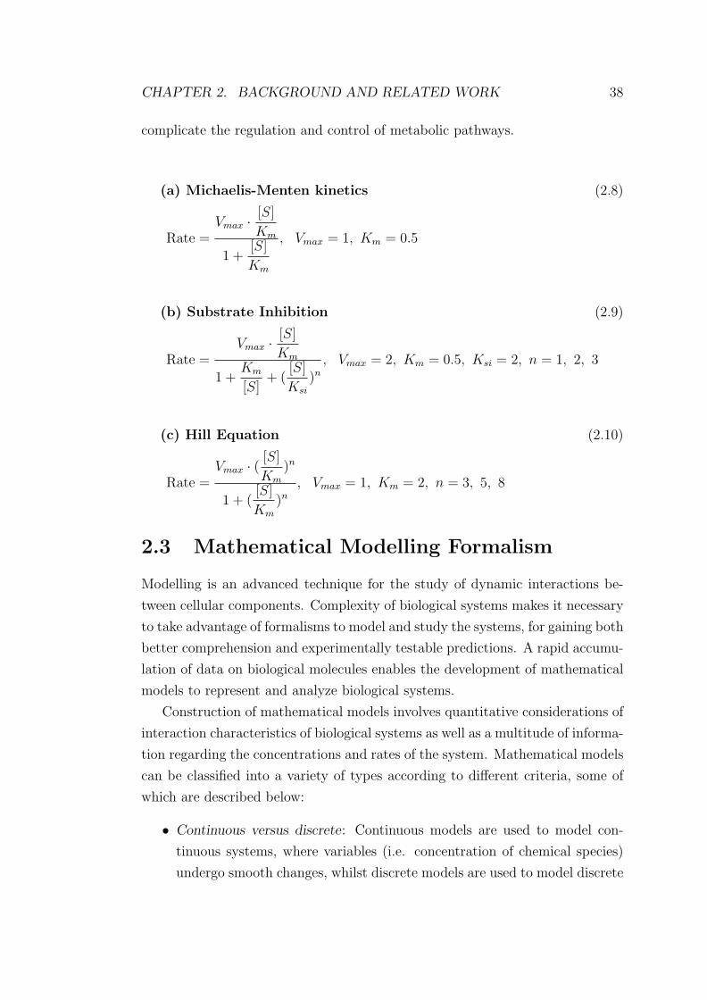
Figure 2.1 presents three typical shapes of the dependence of enzymatic
velocity on substrate concentration, including the standard Michaelis-Menten
mechanism, substrate inhibition and the Hill function.
Conceptually, any substrate that causes a decrease in the production state of
product as its concentration increases will lead to a reaction that displays sub-
strate inhibition kinetics (shown in Figure 2.1(b)). The Hill function corresponds
to a particular biological phenomena – cooperative binding. In cooperative bind-
ing, the binding of the substrate at one site (of an enzyme with multiple active
sites) increases or decreases the affinity for the substrate at other sites. This
is defined as positive cooperativity and negative cooperatively, respectively. As
shown in Figure 2.1(c), when the Hill coefficient n gets higher, a steeper non-
linearity is produced. In the cases of substrate inhibition and Hill equation,
values assigned for n are for illustrative purposes only.
Rate expressions corresponding to the curves are given in Equations (2.8)
to (2.10). From these components, metabolic pathways can produce regulatory
dynamics of great complexity. Many enzymes in metabolic pathways are subject
to feedback regulations, where an end-product activates or inhibits the enzyme
activity by binding to a separate site. A variety of feedback loops can further

CHAPTER 2. BACKGROUND AND RELATED WORK 37
0 1 2 3 4 5Substrate (mM)
0
0.2
0.4
0.6
0.8
1
Rat
e (m
M/m
in)
(a) Michaelis-Menten mechanism
0 1 2 3 4 5Substrate (mM)
0
0.5
1
1.5
Rat
e (m
M/m
in)
n=1n=2n=3
(b) Substrate Inhibition
0 1 2 3 4 5Substrate (mM)
0
0.2
0.4
0.6
0.8
1
Rat
e (m
M/m
in)
n=3n=5n=8
(c) Hill Equation
Figure 2.1: Three typical shapes of the dependence of the enzyme velocity on thesubstrate concentration (in the range 0 to 5 mM) are shown schematically. (a):Michaelis-Menten mechanism. (b): Michaelis-Menten mechanism plus substrateinhibition with n = 1 (continuous line), n = 2 (dotted line), and n = 3 (segmentand dotted line). (c): Hill equation with n = 3 (continuous line), n = 5 (dottedline), and n = 8 (segment and dotted line). The three rate expressions are givenin Equations (2.8) to (2.10).

CHAPTER 2. BACKGROUND AND RELATED WORK 38
complicate the regulation and control of metabolic pathways.
(a) Michaelis-Menten kinetics (2.8)
Rate =Vmax · [S]
Km
1 +[S]
Km
, Vmax = 1, Km = 0.5
(b) Substrate Inhibition (2.9)
Rate =Vmax · [S]
Km
1 +Km
[S]+ (
[S]
Ksi
)n, Vmax = 2, Km = 0.5, Ksi = 2, n = 1, 2, 3
(c) Hill Equation (2.10)
Rate =Vmax · ( [S]
Km
)n
1 + ([S]
Km
)n, Vmax = 1, Km = 2, n = 3, 5, 8
2.3 Mathematical Modelling Formalism
Modelling is an advanced technique for the study of dynamic interactions be-
tween cellular components. Complexity of biological systems makes it necessary
to take advantage of formalisms to model and study the systems, for gaining both
better comprehension and experimentally testable predictions. A rapid accumu-
lation of data on biological molecules enables the development of mathematical
models to represent and analyze biological systems.
Construction of mathematical models involves quantitative considerations of
interaction characteristics of biological systems as well as a multitude of informa-
tion regarding the concentrations and rates of the system. Mathematical models
can be classified into a variety of types according to different criteria, some of
which are described below:
• Continuous versus discrete: Continuous models are used to model con-
tinuous systems, where variables (i.e. concentration of chemical species)
undergo smooth changes, whilst discrete models are used to model discrete

CHAPTER 2. BACKGROUND AND RELATED WORK 39
systems where changes in variables occur in discrete steps (i.e. number of
molecules or a countable number of points in time).
• Deterministic versus stochastic: Given a fixed set of initial conditions, a
deterministic model always produces the same output, whilst a stochastic
model takes randomness or probability distributions into account such that
for a given input, the outcome of the model is not uniquely determined
but takes a range of possible values.
• Static versus dynamic: Models are said to be dynamic if their behaviour
varies with time, and time therefore enters as an independent variable (i.e.
differential equation). Models are static if their behaviour is constant and
does not vary with time (i.e. mass-balance equations).
• Quantitative versus qualitative: Quantitative models are designed to study
time dependent behaviour, whereas qualitative models are mainly used to
identify high-level properties, such as structure and global functions of
biological systems. Qualitative models may contain quantitative variables,
which are however used for qualitative rather than numerical reasoning
about relationships between system components.
In this thesis, we focus on continuous deterministic mathematical models by
means of ordinary differential equations (ODE), which are a widespread formal-
ism to model dynamic systems in science and technology. The ODE formalism
models time-dependent behaviour of system variables with respect to the inde-
pendent variable. In the context of biology, the independent variable is usually
time and dependent variables (so-called state variables) are measurable quan-
tities (i.e. concentrations of biological entities), which have non-negative val-
ues. Models defined with ODEs have been employed to quantitatively analyze
metabolic pathways, for example, the glycolysis pathway in bloodstream-form
Trypanosoma brucei (Bakker 1998), the polyamine metabolic pathway in mam-
malian cells (Rodriguez-Caso et al. 2006) and the glutathione metabolic pathway
in liver cells (Reed et al. 2008). ODE-based modelling and simulation has also
been performed on the ERK (Extracellular Signal Regulated Kinase) cascade
of the MAPK (Mitogen-Activated Protein Kinase) pathway, which transduce a
variety of external signals to generate a wide range of cellular responses (Orton
et al. 2005).

CHAPTER 2. BACKGROUND AND RELATED WORK 40
In this section, we give a detailed explanation of ODE-based modelling tech-
niques. However, an alternative technique of stochastic modelling is also outlined
for the sake of comparison. Generally speaking, stochastic approaches are used
to model components that are present in small molecule numbers (i.e. promot-
ers and transcription factors), whilst deterministic approaches are suitable when
components are present in high concentrations (i.e. proteins).
2.3.1 Ordinary Differential Equations
Dynamic cellular processes are frequently described using sets of differential
equations. Of all types of differential equations, ODEs are the most commonly
used technique to describe and explore dynamics of a specified natural system,
in particular, in the modelling and analysis of biological systems.
Equations relating an unknown function and one or more of its derivatives
is called a differential equation (Ascher et al. 1995). Studying system behaviour
by means of differential equations comprises the following steps:
• to formulate the differential equation that can describe a specific system
• to find an appropriate solution of that equation
• to understand the system by interpreting the solution
Construction of an ODE model of metabolic pathways is illustrated by an
example. Consider the simple metabolic pathway:
Ssυ1−→ Si
υ2−→ Sp (2.11)
where Si is the intermediate component of the pathway, concentrations of which
can vary depending on enzyme activities and concentration of substrate (Ss)
and product (Sp). Intracellular chemical reactions are catalyzed by enzymes Es1
and Es2 at rates υ1 and υ2 respectively. The differential equation of the state
variable Si is expressed as the difference of incoming and outgoing rate velocities
governed by a specific kinetic law (i.e. Michaelis-Menten kinetics)
d[Si]
dt= υ1 − υ2 (2.12)
Due to the non-linear nature, computational calculation is required to in-
tegrate differential equations in order for essential information underlying the

CHAPTER 2. BACKGROUND AND RELATED WORK 41
model structure to be properly interpreted. General methods of numerical inte-
gration include the Euler method and Runge-kutta Method; relevant materials
are available elsewhere (see Press et al. 2002).
A large number of software tools have been developed for the simulation of
dynamic models specified in terms of ODEs. The software tools differ in two
aspects, including the underlying techniques applied and capabilities supported.
Matlab is a general-purpose mathematical environment that is widely used in the
physical and engineering sciences. A major benefit of the Matlab environment
is the comprehensive library of mathematical and graphical functions, enabling
convenient visualization, analysis and optimization of biological models. A com-
prehensive review on modelling tools and resources is given by Gilbert et al.
(Gilbert et al. 2006).
2.3.2 Stochastic Master Equations
The number of molecules participating in elementary reactions can vary by or-
ders of magnitude (Shampine et al. 2000). ODEs are appropriate to model
systems with a large number of molecules involved, in which case the reaction
probability can be assumed to be independent of the details of collisions between
molecules. When modelling biological systems that contain only a few molecules,
the discrete nature of the number of molecules cannot be ignored. It thus may
be useful to develop models that are both discrete and stochastic in order to
accurately describe the random occurrence of molecule collisions. One of the
frequently used models is stochastic master equations, which has the potential
to describe a wide range of phenomena.
The stochastic formalism decompose biological pathways into elementary re-
actions with probabilities are variables to describe the state of the system. A
joint probability distribution, P (X1, . . . , XN , t), is determined by the probabil-
ity of individual molecular species i having Xi number of molecules. Suppose
that there are M different reactions in the system, the change over time of
the probability distribution is expressed in the following equation, based on the
descriptions given by Baldi and Hatfield (Baldi and Hatfield 2002):
P (Xi, . . . , XN , t + Δt) = P (Xi, . . . , XN , t)
(1 −
M∑j=1
αjΔt
)+
M∑j=1
βjΔt (2.13)
where αjΔt is the probability that reaction j will occur in the interval Δt given
CHAPTER 2. BACKGROUND AND RELATED WORK 42
the system in the state X1, . . . , XN at time t and βjΔt is the probability that
reaction j will bring the system to the state X1, . . . , XN in the interval Δt.
Taking the limit as Δt → 0 gives the master equation, which describes the
probability distribution of all possible states at all times, defined as follows:
∂P
∂t=
M∑j=1
(βj − αjP ) (2.14)
Using analytical methods to analyze the master equations would be extremely
difficult, given the amount of information required for the stochastic formalism
(i.e. the number of chemical species involved and the number of molecules
each species contains). Stochastic simulation techniques, for instance, Gillespie’s
method (Gillespie 1977), are required to solve the equations.
Overall, ODE models and stochastic models are concentrated on different
objectives when studying dynamic systems. As stated by de jong (de Jong 2002),
ODEs determine the transient changes of system variables with respect to time,
whilst master equations examine the probability that a shift in the state of the
system occurs.
2.3.3 Computational Simulation
Computational simulation is an essential tool for the study of complex systems,
where a purely empirical approach is infeasible. The type of simulation ap-
plied should correspond to the type of mathematical model to be solved. In
stochastic simulations, concentrations (in terms of numbers of molecules) are
treated as random variables. In contrast, ODE-based approaches are determin-
istic and concentrations are obtained by solving the differential equations (Ullah
et al. 2006). By means of computational simulation, an intuitive impression
of how these equations relate to dynamic responses can be gained. With valid
models, simulation results are able to make predictions about possible behaviour
of biological systems (Endy and Brent 2001).
There can be many circumstances where computational simulation is neces-
sary. Neelamkavil (Neelamkavil 1987) stated that simulation is necessary when
there is a need to study the past, present, or future behaviour of the system
in real time, such as side-effects of new drugs. Computational simulation en-
ables us to investigate the sensitivity of biological systems to parameter changes
such as environmental noise and minor mutations (Liu et al. 2008). Kitano
CHAPTER 2. BACKGROUND AND RELATED WORK 43
(Kitano 2002a) highlighted that noise tolerance is exhibited by several biolog-
ical systems that feature oscillatory behaviour and transcriptional regulations,
however the degree of tolerance can only be quantitatively evaluated using com-
putational simulations. For example, the robustness of segmentation during
Drosophila embryogenesis in response to various kinetic parameters has been
investigated via computational simulation (von Dassow et al. 2000).
Exploration of the time-dependent behaviour of biological processes is one of
the most frequent applications of dynamic models (Wiechert 2002). Huang and
Ferrell (Huang and Jr. 1996) developed differential equation models of MAPK
signalling pathway to study the role of negative feedback mechanisms in gov-
erning ultrasensitivity in the pathway. Mechanisms regulating MAPK pathway
dynamics were further examined by Asthagiri and Lauffenburger (Asthagiri and
Lauffenburger 2001), where the authors implemented feedback mechanisms in a
mathematical model of the pathway and demonstrated that with negative feed-
back regulations, the model yielded a complete signal adaptation to its direct
target. Cho et al. (Cho et al. 2003) developed an ODE model to investigate the
influence of RKIP (the Raf Kinase Inhibitor Protein) on ERK signalling path-
way. Refer to (Hoppensteadt and Peskin 2002) for more interesting applications.
Mathematical models are a valuable tool for organising data and the exami-
nation of complex biological interactions (Bailey 1998). In the context of biology,
mathematical models integrate biological data at various levels (including tran-
scriptome, proteome and metabolome) and provide an unambiguous description
of biological systems. A mismatch between simulation results and experimental
observations can indicate deficiencies in the model, suggest modifications to the
model and guide new biological experiments. For example, as found by Orton et
al. (Orton et al. 2005), computational simulation of the Schoeberl MAPK model
(published by Schoeberl et al. (Schoeberl et al. 2002)) revealed that the negative
feedback loop from ERK-PP to SOS is necessary. Developing sound models with
predictive power is central to the domain of computational modelling.
After a valid model is constructed, formal analysis can be carried out to
study interesting properties of the system. Model analysis comes into various
forms with different objectives. It can be used to understand system structure
or to investigate system dynamics. In reality, analysis of dynamics and structure
are overlapping processes and are beneficial to each other (Kitano 2002b).
Application of analytical methods depends on the amount and type of biolog-
ical knowledge incorporated in the model (Kitano 2002b). For example, static
CHAPTER 2. BACKGROUND AND RELATED WORK 44
models that are based on graph theory are completely adequate for steady-state
analysis, since only the network topology is required. However, static models
are incompatible with simulation-enabled analyses (e.g. parameter sensitivity
analysis), where a dynamic descriptions of the system is necessary.
2.4 System Identification
System identification is defined by Ljung (Ljung 2008) as “the art and science
of building mathematical models of systems from observed input-output data”.
Two broad branches of system identification are Structure Identification and
Parameter Estimation (Soderstrom and Stoica 1989). Structure identification is
concerned with finding a suitable model structure, within which a good model
is to be decided upon, and parameter estimation deals with, given a structure
and a set of experimental data, how the model can be fitted to observation data
in the best possible way. In this section, we focus on the subject of structure
identification. Computational issues associated with global optimization in the
context of single-objective optimization are studied in detail in Chapter 5. A
multi-objective optimization approach for parameter estimation is investigated
in Chapter 6.
According to different levels of initial knowledge about the system and the
purpose of modelling, mathematical model representations can be classified into
three general categories, which are described in generic terms below and as
summarized in the reviews (Ljung 2007, Sontag 2006, Sjoberg et al. 1995).
1. White Box model: This is the case when physical insight about the system
is complete and all the conditions are known quantitatively, indicating that
it is possible to construct the model entirely from prior knowledge.
2. Black Box model: This is the case when no physical insight is available or
used. A black-box model is a parametrized description of the process, and
all parameters are estimated from measurements performed on the process
without taking into account any prior knowledge about the process.
3. Grey Box model: This is the case when physical insight about the system
is incomplete and unknown quantitative conditions have to be determined
from observed data. According to the type and level of information avail-
able for the task, grey-box models can be further divided into the following
sub-classes:

CHAPTER 2. BACKGROUND AND RELATED WORK 45
• A mechanistic description of the system can be built on existing phys-
ical knowledge about the system (i.e. rate laws and interconnection
relationships). When the model structure is defined, the identifica-
tion process is then to estimate the parameters from observed data,
which are unknown physical constants in the description.
• Mechanistic descriptions can be only obtained for some elementary
parts of the system. To construct an entire model, black-box struc-
tures representing non-linear transformations between system com-
ponents are necessary to approximate the ambiguously defined or
unknown dynamics.
The idea of designing white-box models (so-termed mechanistic models) is
to base the model construction on physical cellular functions, thus the results
of model simulation and prediction can be directly applied to actual biological
systems. The development of white-box models in order to understand the sys-
tems of life is the fundamental question addressed by computational systems
biology (Kitano 2002a). A detailed description of biological systems allows the
performance of simulated experiments to predict unobserved properties. How-
ever, a major weakness of this approach is the empirical nature and the essential
relations are often difficult to extract (Heinrich et al. 1977). Constructing a
white-box model for complex dynamic systems is an extremely difficult task as
in most cases the knowledge about the system is at best partial.
System identification is concerned with the development and analysis of
methods for performing black-box modelling (Soderstrom and Stoica 1989). The
black-box model representations appear to be more beneficial in modelling bi-
ological applications that are poorly defined. Black-box models are relatively
easy to construct and use (Soderstrom and Stoica 1989), and can be approx-
imated in the form of, for example, power series polynomials, fuzzy logic or
neural networks. A difficult problem in system identification is to find an appro-
priate mathematical form, in particular when the dynamics of the system are
non-linear.
Basically, black-box modelling looks for a relationship between past observa-
tions and future outputs. The area of black-box modelling is very diverse, and
covers topics from mathematical approximation theory; specifically, estimation
theory, regression and classification methods (Sjoberg et al. 1995).
Sontag et al. (Sontag et al. 2004) attempted to determine reaction mecha-

CHAPTER 2. BACKGROUND AND RELATED WORK 46
nisms of biological systems from the measurements of time-course species con-
centrations. The authors developed quantitative techniques to identify causal
relationships between species by monitoring time-dependent cellular responses
to perturbations. The basic idea is to analyze the direct effect of a small change
in one network node on the activity of another node, while keeping all remain-
ing nodes fixed. The network responses to perturbations are estimated using the
partial derivatives that quantify the influence of each variable upon the rate of
change of other variables. The big advantage of this approach is that it is also
applicable to the situations where some network nodes cannot be perturbed;
this limit is tackled by applying more independent perturbations to other nodes
to which perturbations are allowed. Thus, an increase in the node connections
does not necessary change the number of required perturbation experiments and
calculations.
Gardner et al. (Gardner et al. 2003) applied multiple linear regressions to
the system identification of a nine-gene sub-network of the SOS pathway in Es-
cherichia coli. Regulatory coefficients for each pairs of genes were determined,
whereby the interconnection map and the key regulatory functions between gene
products in the network were identified. In the work by Gardner et al., no prior
knowledge was claimed to be necessary, but still 36 combinations of seven per-
turbations was used. Geier et al. (Geier et al. 2007) addressed the problem of
model construction of gene-regulatory networks from knockout data. The au-
thors compared the performance of different network reconstruction methods and
investigated the impact of data size and observation noise on the construction of
gene regulatory networks. They found that error rates during the construction
process increased with an elevation in the noise level and a decrease in the data
size.
Moreover, Crampin et al. (Crampin, McSharry and Schnell 2004) and Sriv-
idhya et al. (Srividhya et al. 2007) considered the problem of inferring kinetic
mechanisms for chemical reactions from time series data using polynomial mod-
els of chemical reactions based on mass action kinetics. Kocijan et al. (Kocijan
et al. 2003) also took advantage of the black-box identification approach formu-
lated as a Gaussian process model to study the model-based predictive control
problem. Refer to the works (Lauwers et al. 2007, Liu and Wang 2008, Kemna
and Mellichamp 1995) for more examples of the system identification of biolog-
ical systems.
The biggest disadvantage of model construction via black-box modelling is

CHAPTER 2. BACKGROUND AND RELATED WORK 47
the implicit relationship with physical reality (Heinrich et al. 1977). This is to
say that any arbitrary black-box model can be made to fit experimental ob-
servations, however this does not necessarily mean that they represent a phys-
ically correct model of the system. Soderstrom and Stoica (Soderstrom and
Stoica 1989) pointed out that models obtained by system identification in some
cases have limited validity (for example, they are valid only for a certain working
point) and parameters included are used only as tools to give a good description
of the system’s behaviour. The amount of available experimental data and the
non-linearity of biological systems are the deciding factors when selecting an
appropriate model approximation. An overview of system identification tech-
niques for model construction from time series data is given by Crampin et al.
(Crampin, Schnell and McSharry 2004).
In contrast, grey-box modelling can relieve some of the drawbacks arising
from black-box modelling and still maintain dynamical flexibility (Tan and Li
2002, Oussar and Dreyfus 2001). We consider grey-box models as a combination
of white-box and black-box models. Tulleken (Tulleken 1993) argued that grey-
box modelling can benefit the advanced control design, which requires a model
that can adequately describe the mechanisms of the underlying process. Tulleken
proposed an approach to solve the problem of statistical estimation where a
linearly parametrized dynamic regression model was used. Tan and Li (Tan and
Li 2002) employed Pade approximation in the form of a regressive function as
the black-box structure to solve two non-linear chemical processes. Tullenken
(Tulleken 1991) applied this type of modelling to the model construction of a
batch reactor system and indicated that the grey-box strategy could improve
the statistical identification results considerably.
As highlighted by Heinrich et al. (Heinrich et al. 1977), there are compro-
mises among the three modelling representations in the use of models that are
as simple as possible, yet are still consistent with the real system. Simplification
of a model can be achieved through the reduction of the number of variables or
parameters. One useful model reduction technique is based on topological reduc-
tion of metabolic pathways, through which adjacent reactions may be lumped
into a single overall reaction (Heinrich et al. 1977). This technique is applied in
the structural modelling of the trypanothione metabolism in Chapter 3.
In summary, a sound metabolic model is necessary for achieving a global
understanding of the capabilities of metabolic processes. However, no auto-
matic reconstruction methods can be directly used to discover currently un-

CHAPTER 2. BACKGROUND AND RELATED WORK 48
known metabolic reactions (Breitling et al. 2008). Breitling et al. summarized
a number of technological advances that could allow de novo reconstruction of
large unexplored parts of the metabolic map directly from experimental obser-
vations. Breitling et al. (Breitling et al. 2008) highlighted a high-accuracy mass-
spectrometry approach, which has been applied to the study of T. brucei. The
authors argued that this approach can accurately predict the potential connec-
tivity between related metabolites, thus enables a precise de novo reconstruction
of an entire hypothetical metabolic map. Recently developed software by Jour-
dan et al. (Jourdan et al. 2008) enables visualization of mass-spectrometry data
obtained from this method and allows basic analysis of the resulting network.
In many instances, sufficient physical knowledge and quantitative informa-
tion for constructing a mechanistic mathematical model of the entire system is
difficult or impossible to obtain. We take advantage of the concept of grey-
box models in the kinetic modelling of a sub-pathway of the trypanothione
metabolism (the polyamine biosynthetic sub-pathway), as illustrated in Chap-
ter 7. Within the grey-box model, a white-box representation is applied to de-
scribe known physical properties of the system and a black-box representation
is used to approximate the unknown dynamics.
2.5 Network Modularity
Cells can be seen as composed of a large number of self-contained reaction sub-
systems, so-called ‘modules’, which carry out specific biological processes. Cell
behaviour thus can be understood in terms of ‘modules’ interacting via cas-
cades and feedback regulations in a complex web, which is defined by Sontag et
al. (Sontag 2006) as one of the important themes in current molecular biology.
Sub-systems can be thought of as black boxes that process time-dependent in-
put signals (i.e. forcing functions) or external signals (i.e. stimuli) into output
responses (i.e. measurements provided by biological reporter devices). Model
decomposition techniques facilitate the study of emergent properties of intercon-
nections, thus benefiting the model construction of large-scale biological systems
on modular bases (Kholodenko et al. 2002).
From the perspective of molecular biology, a module can be considered as a
group of biological components that are spatially isolated and/or functionally
independent, and classified as topological and functional modules, correspond-
ingly. From a purely topological perspective, hierarchical modularity is evident

CHAPTER 2. BACKGROUND AND RELATED WORK 49
in metabolic networks in all organisms (Ravasz et al. 2002). Topology-based
modules are comparatively straightforward to derive. Since they are based on
graph theory, minimal prior knowledge about biological function or evolution is
required.
Centrality is a core concept for the study of topological modules. Edge be-
tweenness is the most prominent measure of centrality, which determines the
relative importance of an edge within a graph, and therefore the density of
sub-networks of a complex network system (Girvan and Newman 2001). The
measure of edge betweenness favors edges lying between sub-networks and dis-
favors edges lying inside sub-networks. There are various implementations of
this measure. One of the standard variants is shortest-path betweenness, which
finds the shortest paths between all pairs of vertices and counts how many run
along each edge (Newman 2001). Zhao et al. (Zhao et al. 2007) applied this
decompositional approach to examine the co-evolution of topological modules
of metabolic networks in H. sapiens, where they used the simulated annealing
algorithm proposed in (Guimera and Amaral 2005) to develop the modules. In
spite of the prevalence of topological modularity in networks, network modu-
larization should rely on functional characterization of biological components
(Sauro et al. 2006). Hartwell et al. (Hartwell et al. 1999) argued that the iden-
tification of functional modules is a crucial level of abstraction in the modelling
of biological systems. However, how to functionally modularize a network is the
key problem.
Ravasz et al. (Ravasz et al. 2002) proposed a decompositional approach
for the classification of topological modules, where clustering coefficients among
substances are calculated to determine the number and degree of clustering. The
coefficients reflect the The authors attempted to establish a relation between
topological modules and the known functional properties of the metabolites,
and pointed out that biological verification of the relation remains to be the
critical issue. Further experiments and theoretical analyses are needed in order to
understand the potential relation between the identified hierarchical architecture
and functionally relevant sub-networks.
The concept of modularity has been applied to solve the parameter estimation
problem of biological systems, by which the complexity of the problem can be
largely reduced. Van Riel and Sontag (van Riel and Sontag 2006) developed a
‘dependent-input’ approach for the identification of unknown system parameters.
This approach allows a part of the system to be studied independent of the rest
CHAPTER 2. BACKGROUND AND RELATED WORK 50
of the cell by replacing the un-modelled dynamics (of the rest of the system)
with the measured dependent inputs. A critical challenge with regard to the
use of the ‘dependent-input’ approach lies in how to represent the modules to
render the predictive power, since the ultimate goal is not only to examine the
underlying assumptions but also to make predictions to be tested experimentally.
Bentele et al. (Bentele et al. 2004) took advantage of network modularity for
parameter estimation in the apoptotic signalling network. Sensitivity analysis
that describes changes of molecule concentrations as result of changes in the
values of parameters (so-called local sensitivity analysis) is applied to identify
clusters that contain a subset of molecules whose concentrations depend on a
subset of parameters only. The parameter estimation problem was solved via
a two-level hierarchy, where at the upper level, global parameters that belong
to more than one cluster are estimated and at the lower level, remaining local
parameters belonging to individual subsets are estimated separately from each
cluster. At the lower level, estimation of the local parameters is dependent
on the values of the global parameters solved from the upper level. However,
this approach may be computationally expensive, as sensitivity analysis has to
be performed and evaluated within the parameter estimation space after each
iteration step.
In summary, network modularity provides a convenient way to examine the
relationship between topological and functional building blocks that accomplish
specific cellular functions, which assists in the analysis of system behaviour and
exploration of unknown systemic properties. Within a ‘modular’ framework,
the challenge of understanding the complex network of molecular interactions
can be facilitated (Lauffenburger 2000). We take advantage of the concept of
network modularity in the modelling of the trypanothione metabolic pathway.
In Chapter 7, we propose an optimization-based decompositional approach that
is different from the previously discussed approaches to guide the investigation
of model structure correctness of the pathway.
2.6 Discussion
The study of biological pathways is becoming the reference framework for under-
standing the dynamics of many intercellular and intracellular processes. As most
pathways of interest involve components connected through interlocking loops,
an intuitive understanding of their dynamics is hard to obtain. It is therefore

CHAPTER 4. INITIAL KINETIC MODEL 101
in the concentration will give rise to a concomitant increase in the enzyme ac-
tivity. There are three types of inhibitors, called competitive, noncompetitive
and uncompetitive. These inhibitors represent a similar pattern in regulating
enzyme kinetics of chemical reactions. For a simple reaction S + E −→ P ,
the Michaelis-Menten kinetic scheme can be formulated correspondingly. As un-
competitive inhibitors are not common and are difficult to design (Eisenthal and
Cornish-Bowden 1998), the trypanothione metabolic pathway is limited to the
following modes of regulation.
• Competitive Inhibition
Rate =kcat · E · S
Km
1 +S
Km
+I
Ki
• Noncompetitive Inhibition
Rate =kcat · E(
1 +I
KI
)γi· S
Km + S
• Substrate Inhibition
Rate =kcat · E
1 +Km
S+
S
Ksi
• Product Activation
Rate =kcat · E(
1 +Ka
A
)γa· S
Km + S
In the above schemes, kcat represents the turnover number, expressed as
number of substrate molecules turned into product per enzyme site per time
unit. E and Km are the total enzyme concentration and the half-saturation
constant. Ki and Ka stand for the inhibitory and stimulating effect chemical
compounds I and A exert on the enzyme activity, respectively. A regulatory
term can be regarded as the concentration of chemical compounds divided by
activation or inhibition constant. Apart from the scheme of substrate inhibition,

CHAPTER 4. INITIAL KINETIC MODEL 102
when the regulatory terms are set to zero, the above rate equations give identical
kinetics to the standard Michaelis Menten. The parameters γi and γa represent
the strength of inhibition and activation, respectively.
Structural analysis in Chapter 3 implies that the trypanothione metabolism
in T. brucei is composed of two fundamental building blocks, including trypan-
othione biosynthesis and trypanothione redox system. These two building blocks
appear to be spatially isolated in the network topology. This shows an agreement
with observations in the study by Ravasz et al. (Ravasz et al. 2002) that cellular
metabolism is best represented with a hierarchical and modular network. The
hierarchical layout of the trypanothione pathway in T. brucei provides a natural
breakdown of metabolism into relevant sub-networks. Further discussion on the
subject is given in Section 7.8 in Chapter 7.
In the rest of this chapter, we summarize the model description for individual
sub-networks responsible for the trypanothione biosynthesis and the trypanoth-
ione redox system. Trypanothione biosynthesis is achieved through integration
of two elementary sub-pathways carrying out specific cellular functions, namely
the polyamine biosynthetic sub-pathway and the glutathione biosynthetic sub-
pathway. The trypanothione redox system is comprised of two metabolic pro-
cesses, including the trypanothione oxidation and regeneration and the formation
of NADPH and pentoses.
4.3.1 Polyamine Biosynthesis
Polyamines are ubiquitous cellular components essential for cell growth and di-
vision. In mammalian cells, the most common polyamines are putrescine, sper-
midine and spermine. ODC catalyses the initial step in the pathway leading to
putrescine production from ornithine. In the presence of the aminopropyl donor
decarboxylated AdoMet (dAdoMet), spermidine and spermine are synthesized
from putrescine under the catalysis of spermidine synthase and spermine syn-
thase respectively. AdoMetDC catalyses the conversion of S-adenosylmethionine
(AdoMet) to the methyl donor dAdoMet.
ODC and AdoMetDC are rate-limiting enzymes that can be rapidly induced
by various growth stimuli. A comprehensive review on T. brucei ODC and
AdoMetDC can be found in (Persson 2007).
One primary use of polyamines in bloodstream-form trypanosomes lies in
the formation of the conjugate GspdSH, which is an essential substrate for

CHAPTER 4. INITIAL KINETIC MODEL 103
trypanothione biosynthesis. It has been shown that trypanosomes depend on
spermidine for growth and survival, which ceases when spermidine level drops
below a certain level (Heby et al. 2007). There is therefore considerable thera-
peutic potential in compounds that disrupt polyamine biosynthesis (Wallace and
Fraser 2004, Marton and Pegg 1995, Bacchi and Yarlett 2002, Kaiser et al. 2003).
The antiparasitic drug, DFMO, for example, functions in a way that irreversibly
interacts with ODC to reduce polyamine levels.
There is a dependence between levels of polyamines and viability and growth
of parasites. In the parasitic organism L. donovani, polyamine supplementa-
tion can rescue intracellular pools of Δadometdc (Roberts et al. 2002), Δodc
(Jiang et al. 1999) and Δspdsyn (Roberts et al. 2001)1. Unexpectedly, over-
expression of the enzymes did not proportionally increase polyamine content
(Roberts et al. 2007). It was found that lack of spermine (Kaur et al. 1986)
and/or an increase in spermine pool (Ariyanayagam and Fairlamb 2001, Fair-
lamb et al. 1987, Bellofatto et al. 1987) did not affect trypanosomal growth
rate. We therefore excluded spermine production from the model owing to its
negligible role in the regulation of trypanothione metabolism.
Polyamine metabolism in mammalian cells has been studied using mathe-
matical modelling (Rodriguez-Caso et al. 2006). The major differences between
polyamine metabolism in mammals and trypanosomes lie in the specificity of
metabolites and enzymes as well as the associated regulation patterns. The
model of polyamine biosynthesis in T. brucei considers the enzyme activities
and polyamine concentrations extracted from experimental studies. T. brucei
lackes the capacity to assimilate exogenous performed radioactive putrescine and
spermidine (Bacchi et al. 1980, Taylor et al. 2008). The polyamine biosynthetic
sub-pathway takes exogenous methionine and arginine as inputs for the produc-
tion of downstream metabolites. We also incorporate the enzymatic reaction
converting AdoMet in S-adenosyl-L-homocysteine (AdoHcy) under the catalysis
of methyltransferases due to its potential role in regulating AdoMet dynamics.
The polyamine biosynthetic sub-pathway is described mathematically by a
set of rate equations for each of the T. brucei enzymes.
ODC Ornithine, putrescine and spermidine are metabolites common to both
mammalian cells and trypanosome parasites. The major difference between
enzyme ODC in the two families of organisms lies in their turnover rates (Persson
1Δ stands for the enzyme knockout strains of parasites.

CHAPTER 4. INITIAL KINETIC MODEL 104
et al. 2003). ODC has an extremely short intracellular half-life in mammals,
reportedly 15 min to 1 hr, which is in contrast to the more stable protein in T.
brucei with a turnover rate greater than 6 hrs. As indicated by Ghoda et al.
(Ghoda et al. 1990), the stability of T. brucei ODC results from the lack of the
L-terminal PEST sequence (proline, glutamate, serine and threonine) necessary
for rapid degradation and polyamine-dependent regulation.
Rapid turnover allows the enzyme to respond to regulatory stimuli promptly.
Hayashi and Murakami (Hayashi and Murakami 1995) reported that exogenously
added polyamines accelerated repression and destabilization of ODC activity in
mammalian cells. On the contrary, T. brucei ODC activity in the procyclic form
is unaffected by putrescine and spermidine, which indicates that the mechanism
for polyamine-mediated regulation may be absent (Hua et al. 1995). The same
argument with regard to the unresponsiveness of T. brucei ODC to polyamines
was also made by Ghoda et al. (Ghoda et al. 1992). A conflicting experimental
observation, however, reported by Osterman et al. (Osterman et al. 1994), which
indicated that putrescine inhibited ODC with an inactivation coefficient equal to
350±43 μM. The experimental work performed by Osterman et al. is considered
as a relevant data source to our study for its known validity.
A mathematical rate expression for ODC is modelled in the form
VODC = kODCcat · [ODC] ·
[Orn]
KODCmOrn
1 +[Orn]
KODCmOrn
+[Put]
KODCiP
(4.1)
where kODCcat is the turnover number, and KODC
mOrn stands for the half-saturation
constant of the enzyme by ornithine (Orn). KODCiP is the constant of competi-
tive inhibition by putrescine (Put). Square brackets [ · ] stand for intracellular
concentrations of the corresponding metabolites. The same notation scheme is
applied to other equations below.
In the presence of DFMO, ODC is irreversibly deactivated. A modified ex-
pression of the dynamic velocity of ODC is written below:
V DFMOODC = kODC
cat · [ODC]
1 +[DFMO]
KODCiDFMO
·[Orn]
KODCmOrn
1 +[Orn]
KODCmOrn
+[Put]
KODCiP
(4.2)

CHAPTER 4. INITIAL KINETIC MODEL 105
where KODCiDFMO represents the inhibition constant from the inhibitor DFMO.
As ODC activity responds to DFMO in a time and concentration dependent
manner, the dynamics of intracellular DFMO must be known. T. brucei ODC
has a higher KODCiDFMO value of 130 μM for DFMO than that of the mammalian
enzyme (39 μM) (Bitonti et al. 1985). Phillips et al. (Phillips et al. 1988)
reported an even higher value on KODCiDFMO around 160±60 μM. A differential
equation for the transient DFMO concentration is expressed as follows
d[DFMO]
dt= kDFMO
s − kODCd · [DFMO] · V ODC
max
where kDFMOs represents the uptake parameter of the inhibitor and V ODC
max is the
maximum velocity of the enzyme at the normal condition.
However, the DFMO uptake kinetics have not been rigorously characterised
due to a few of factors involved in the process; drug transport and intracellular
distribution, for instance. Procyclic-form T. brucei was reported to take up
DFMO at a linear rate for the initial 60 mins (Phillips and Wang 1987). However,
for simulation of the dynamics of drug-enzyme interactions over 4 days (the
time span considered in model validation), not enough information is available
for an unambiguous characterization of the kinetics of DFMO uptake over the
prolonged time duration.
Despite the absence of a quantitative description, the DFMO-induced sup-
pression of ODC activity is well understood in a qualitative sense. ODC activity
was found to be completely blocked after a certain period of treatment with
DFMO, which caused the amount of putrescine to drop below the experimentally
detectable level (Bacchi et al. 1983, Fairlamb et al. 1987, Bellofatto et al. 1987).
In view of the qualitative knowledge, ODC activity in response to DFMO
is modelled with an exponential decay function below that reflects the time-
dependent pattern of the drug inhibition, expressed as
V ODCmax · e−λ·t (4.3)
where λ stands for the decay rate of ODC under DFMO treatment, and can be
obtained by simple curve fitting, resulting in a value 0.007.
Table 4.1 contains parameter values for T. brucei ODC.
AdoMetDC AdoMetDC is an essential enzyme for the formation of dAdoMet,
the methyl donor for the biosynthesis of spermidine from putrescine. As is the

CHAPTER 4. INITIAL KINETIC MODEL 106
Parameters Description Value/Ranges SourceV ODC
max maximum velocity 45 μmol/min/mg (Phillips et al. 1988)MW molecular weight 45000 (Phillips et al. 1987)kODC
cat turnover rate 444±4.8 min−1 (Osterman et al. 1994)KODC
mOrn half-saturation 160 μM (Bitonti et al. 1985)constant or
280±30 μM (Phillips et al. 1988)KODC
iP inhibition 350±43 μM (Osterman et al. 1994)constant
KODCiDFMO DFMO 220±70 μM (Phillips et al. 1988)
inhibitionλ decay rate 0.007 Analytical Solution
Table 4.1: Parameter values for T. brucei ODC.
case for T. brucei ODC, T. brucei AdoMetDC is a stable enzyme and has a
lower turnover rate than that in mammalian cells. AdoMetDC is a regulatory
enzyme within the polyamine biosynthetic sub-pathway. Regulatory enzymes
can respond to chemical signals with an increase or decrease in their activities.
Metabolic pathways are regulated by controlling the activity of one or more
enzymatic steps along the path. Allosteric control refers to allosteric enzymes
that have distinct binding sites for effector molecules which control their reaction
rates.
AdoMetDC is regulated by an allosteric mechanism with ‘prozyme’, an en-
zymatically inactive close homologue of AdoMetDC iteself. Prozyme induces a
conformational change from an inactive structure to an active one; the bind-
ing of AdoMetDC with prozyme is postulated to enable a dynamical control
on metabolic fluxes through the polyamine pathway (Willert et al. 2007). A
similar mechanism of allosteric regulation was also found for Trypanosoma cruzi
AdoMetDC (Beswick et al. 2006).
Willert et al. (Willert et al. 2007) discovered a regulatory mechanism in
T. brucei that neither AdoMetDC or prozyme per se is sufficiently active to
prompt normal cell growth, and only the complex of AdoMetDC|prozyme can
maintain the physiological level of spermidine. Willert et al. drew a conclusion
that putrescine stimulates the activity of AdoMetDC but has no effect on the
AdoMetDC|prozyme heterodimer.
Recent work by Willert and Phillips (Willert and Phillips 2008) has ex-
tended the subject to examining the influence of AdoMetDC RNAi inhibition

CHAPTER 4. INITIAL KINETIC MODEL 107
and prozyme knockout on polyamine synthesis and parasite growth. In accor-
dance with the study by Willert and Phillips, we elaborate an enzyme-ligand
binding reaction describing the transition of the free inactive conformer (E ′)
into a ligand-occupied active conformer (EL), which complies with the formula
of the total enzyme concentration ET = EO + EL, where L stands for ligand.
EO + L � EOL (4.4)
Prozyme regulates T. brucei AdoMetDC by altering the value of kcat, giving
rise to the so-called ’V-system’, which is in contrast to ’K-system’ that alters
the affinity for substance (Birnbaumer et al. 1980). Here we model the ligand-
enzyme binding reaction as a one-step conformation system, with the assumption
that the ligand can rapidly interact with the enzyme. This assumption makes
sense given the observation that prozyme concentration is not comparable to
the enzyme concentration of AdoMetDC (Willert et al. 2007), giving rise to
the reaction occurring at a rapid-equilibrating rate following the linear mass
action kinetics (i.e. [E]�[S]). Because of the limited amount of prozyme in
parasites, AdoMetDC is present in the cell in both ligand-occupied form and
free form. Accordingly, we express the velocity equation of the total AdoMetDC
as a superposition of two terms stemming from individual form of the enzyme.
The representation of regulatory capabilities in summation of distinct states has
been verified for allosteric enzymes in (Birnbaumer et al. 1980).
AdoMet decarboxylase (AdoMetDC) was reported to be strongly or weakly
activated by putrescine (Bitonti et al. 1986, Tekwani et al. 1992, Willert et al.
2007). Inspection of the details of the experiments that led to these opposing
conclusions showed that different basal levels of putrescine were used by the
different groups and this possibly explains the apparent contradiction. Bitonti
et al. and Willert et al. (Bitonti et al. 1986, Willert et al. 2007) both used crude
extracts rich in putrescine. Tekwani et al. (Tekwani et al. 1992) however used
dialyzed extract without putrescine. In the study of Tekwani et al., addition of
500 μM putrescine gave a 10 fold jump in AdoMetDC activity, which plateaued
at 12 fold enhanced activity with higher concentrations. In vivo putrescine
content was reported at 517 μM (Fairlamb et al. 1987) or 678 μM (Willert and
Phillips 2008), suggesting that the ‘strong’ putrescine activation of AdoMetDC
observed in the study by Tekwani et al. would not be achieved in in vivo
environment. Observations in the works by Bitonti et al. and Willert et al.

CHAPTER 4. INITIAL KINETIC MODEL 108
are therefore considered as relevant data sources to our study.
A mathematical rate expression of the total AdoMetDC is shown below:
VAdoMetDCT = VAdoMetDCL + VAdoMetDCO (4.5)
where VAdoMetDCL and VAdoMetDCO stand for the velocity contributed by the
ligand-occupied and free form of the enzyme, modelled as follows
VAdoMetDCL = kAdoProcat · [AdoMetDCL] ·
[AdoMet]
KAdoPromAdoMet
1 +[AdoMet]
KAdoPromAdoMet
(4.6)
VAdoMetDCO = kAdoMetDCO
cat · [AdoMetDCO] · (4.7)
[AdoMet]
KAdoMetDCO
mAdoMet
1 +[AdoMet]
KAdoMetDCO
mAdoMet
+[dAdoMet]
KAdoMetDCO
idAdoMet
+[KAdoMetDCO
aPut ]
[Put]
where kAdoMetDCO
cat , KAdoMetDCO
mAdoMet and kAdoProcat , KAdoPro
mAdoMet stand for the turnover
rate and half-saturation constant to substrate AdoMet of the free (AdoMetDCO)
and ligand-occupied (AdoMetDCL) form, respectively. Concentration of the
free-form AdoMetDC can be calculated by reducing the total enzyme concen-
tration by the ligand-binding portion
[AdoMetDCO] = [AdoMetDCT ] − [AdoMetDCL]
KAdoMetDCO
aPut and KAdoMetDCO
idAdoMet describe the activation and competitive inhi-
bition exercised by putrescine and dAdoMet. No numbers have been reported
for either parameter in T. brucei. We derived the constant KAdoMetDCO
aPut from
(Bitonti et al. 1986) that gave a value of 1.5 μM. T. brucei AdoMetDC was
thought to be insensitive to dAdoMet, which is in contrast to the strong in-
hibition exerted by dAdoMet on the enzyme in many other species (Pegg and
Jacobs 1983). We apply a range between 1 to 1000 μM to parameter KAdoMetDCidAdoMet
as the quantitative description of T. brucei AdoMetDC in response to product
dAdoMet. The parameter boundaries are wide enough to cover the possibilities
of both weak and strong product inhibition. The parameter estimates from in
silico simulations can be used to qualitatively assess the biological observations.
The formation and dissociation of complex AdoMetDC|Prozyme are de-

CHAPTER 4. INITIAL KINETIC MODEL 109
scribed as an irreversible one-step binding model and a linear decay response,
as shown below
RAdoMetDCL
b = kAdoMetDCL
b · [AdoMetDCT ] · [Prozyme] (4.8)
RAdoMetDCL
d = kAdoMetDCL
d · [AdoMetDCL] (4.9)
where kAdoMetDCL
b and kAdoMetDCL
d stand for the binding and dissociation rate
of the ligand-enzyme interaction. The complex was formed at high affinity with
the dissociation constant smaller than 0.5 μM (Willert et al. 2007); this gives the
functional relation as kAdoMetDCL
d = 0.5 ∗ kAdoMetDCL
b to eliminate one unknown
parameter from the model.
According to the recent experimental observations (Willert and Phillips 2008),
an induction of T. brucei ODC activity was detected when AdoMetDC or
prozyme was inhibited or knocked out. Inhibition of polyamine contents on
ODC activity that has been demonstrated in mammalian cells was not applica-
ble to T. brucei. Willert and Phillips hypothesized that the de-repression of ODC
protein expression could be ascribed to the reduced inhibition by AdoMetDC ac-
tivity, since when AdoMetDC protein expression is diminished, less ODC mRNA
strands would be consumed by AdoMetDC, thus more ODC mRNA could be
translated. Quantitatively, AdoMetDC knockdown induced gene expression of
ODC and prozyme up to an average of 10 to 25 fold the controlled level; exoge-
nous spermidine (100 μM) weakened the stimulating strength but still enabled
5 to 10 fold increases in the enzyme activity. Knockout of prozyme also boosted
ODC expression by 4-5 fold.
To reflect this observation, enzyme ODC is modelled as a variable dependent
on the expression level of AdoMetDC. Equations (4.10) and (4.11) describe the
synthesis term of Prozyme and ODC, respectively, with the expression level of
AdoMetDC and prozyme included in the lower part of the formulas to illustrate
the regulatory effect they exercise.
RProzymes =
(kprozyme
s
1 + [AdoMetDCT ]
)·(
1 +1
[Spd]
)(4.10)
RODCs =
(kodc
s
1 + keq([AdoMetDCT ] + [Prozyme])
)· (4.11)(
1 +1
[Spd]
)RODC
d = kODCd · [ODC] (4.12)

CHAPTER 4. INITIAL KINETIC MODEL 110
where kprozymes and kodc
s represent the production coefficients of prozyme and
ODC, respectively. keq acts as the scaling factor tackling distinct intracellular
amounts of AdoMetDC and prozyme. kODCd is the degradation constant of ODC.
AdoMetDC is a good therapeutic target in T. brucei (Wallace 1996). AbeAdo2,
an enzyme-activated inhibitor of AdoMetDC, was more potent than DFMO
in curing T. brucei infections (Marton and Pegg 1995). In mammalian cells,
dAdoMet does not accumulate under normal conditions because of its rapid uti-
lization in spermidine synthesis. However, DFMO-treated cells display a striking
accumulation of this metabolite due to the lack of putrescine for aminopropyl-
transferase reactions and the elevation of AdoMetDC activity.
In mammalian cells, AdoMetDC activity was detected to elevate threefold
over the normal value within 12 hrs of DFMO addition and then decreased
slightly, with AdoMet staying relatively constant (Mamont et al. 1982). This is
in contrast to drug-treated T. brucei where the levels of AdoMet and dAdoMet
were significantly increased (Fairlamb et al. 1987) concomitant with an approx-
imately 30-70 percent decrease in AdoMetDC activity (Bacchi et al. 1983). Ex-
periments on AdoMetDC down-regulation also revealed a decrease in AdoMet
use for polyamine synthesis and an increase in available AdoMet for tryans-
methylation reactions (Selzer et al. 1996).
Table 4.2 contains parameter values for T. brucei AdoMetDC.
MAT: Methionine Adenosyltransferase In trypanosomes, MAT catalyzes
the synthesis of AdoMet from methionine in the presence of ATP. AdoMet plays
an important role in a variety of cellular functions, such as methylation, sulphu-
ration and polyamine. Polyamines are not inhibitory to the enzyme, and AdoMet
only exercises weak inhibition on the enzyme activity (Yarlett et al. 1993).
Interference with T. brucei polyamine biosynthesis by DFMO resulted in a
dramatic increase in the intracellular AdoMet and dAdoMet pools (Fairlamb
et al. 1987, Bellofatto et al. 1987), and a two-fold increase in AdoMet synthetase
activity in vivo (Yarlett et al. 1991). A mathematical rate expression of AdoMet
synthetase is modelled in the form
VMAT =
⎛⎜⎜⎝
V Metmax · [Met]
KMATmMet
1 +[Met]
KMATmMet
+[AdoMet]
KMATiAdoMet
⎞⎟⎟⎠ ·
⎛⎜⎜⎝
V ATPmax ·
([ATP ]
KMATmATP
)n
1 +
([ATP ]
KMATmATP
)n
⎞⎟⎟⎠ (4.13)
2Systematic name: 5’-{[(Z)-4-Amino-2-butenyl]methylamino}-5’-deoxyadenosine

CHAPTER 4. INITIAL KINETIC MODEL 111
Parameters Description Value/Ranges Source
kAdoMetDCO
cat turnover rate 0.078±0.024 min−1 (Willert et al. 2007)kAdoPro
cat turnover rate 84±6 min−1 (Willert et al. 2007)KAdoPro
mAdoMet half-saturation 110±20 μM (Willert et al. 2007)constant
KAdoMetDCO
mAdoMet half-saturation 380±150 μM (Willert et al. 2007)constant or 30 μM (Bitonti et al. 1986)
KAdoMetDCO
idAdoMet inhibition 1-1000 μM Modellingconstant Assumption
KAdoMetDCO
aPut activation 1.5 μM Analyticalconstant Solution
kb binding 0–10 μM/min Modellingconstant Assumption
kprozymes binding 0–1 μM/min Modelling
constant Assumptionkodc
s synthesis 0–1 μM/min Modellingconstant Assumption
kodcd degradation 0–0.1 μM/min Modelling
constant Assumptionkeq scaling 0–1 μM/min Modelling
constant Assumption[AdoMetDCT ] enzyme 1e-4–1 μM Modelling
concentration Assumption[AdoMetDCO] enzyme 1e-4–1 μM Modelling
concentration Assumption
Table 4.2: Parameter values for T. brucei AdoMetDC.
where kinetic parameters of the enzyme are substrate-concentration dependent;
V Metmax , V ATP
max and KMATmMet, KMAT
mATP denote the maximum velocity and half-saturation
constant for each of the two reactants, respectively. KMATiAdoMet stands for the com-
petitive inhibition by AdoMet. n is the Hill rate of the enzyme activity with
respect to co-substrate ATP.
The maximum velocity of MAT has never been reported in T. brucei, and the
only measurement available for the enzyme was observed in parasitic organism
L. infantum by Reguera et al. (Reguera et al. 2001)3. For this reason, the
enzyme activity of MAT is considered as an unknown parameter during the in
silico simulation of the kinetic model. We thus refined Equation (4.13) by using
a single parameter, V MATmax , to represent the enzyme maximum velocity, which
3MAT with methionine and ATP as substrates were measured to hold the maximum activityof 0.19 μmol/mg/min and 0.12 μmol/mg/min, respectively.

CHAPTER 4. INITIAL KINETIC MODEL 112
results in the rate equation below
VMAT = V MATmax ·
⎛⎜⎜⎝
[Met]
KMATmMet
1 +[Met]
KMATmMet
+[AdoMet]
KMATiAdoMet
⎞⎟⎟⎠ ·
⎛⎜⎜⎝
([ATP ]
KMATmATP
)n
1 +
([ATP ]
KMATmATP
)n
⎞⎟⎟⎠ (4.14)
Table 4.3 contains parameter values for T. brucei MAT. In the model, we
consider ATP as a constitutely supplied protein, since the knowledge concerning
ATP generation and energy conversion with ADP is lacking. ATP concentration
is fixed at its normal cellular value, approximately 4000 μM.
Parameters Description Value/Ranges SourceV MAT
max maximum 1e-3–20 μmol/mg/min Modellingvelocity Assumption
KMATmMet half-saturation 20 μM w.r.t. (Yarlett et al. 1993)
constant [ATP]⊂10-250 μM200 μM w.r.t.[ATP]⊂0.5-5 mM
KMATmATP half-saturation 53 μM w.r.t. (Yarlett et al. 1993)
constant [Met]⊂10-250 μM1750 μM w.r.t.[Met]⊂500-5000 μM
KMATiAdoMet inhibition 240 μM (Yarlett et al. 1993)
constant[ATP ] concentration 4000 μM Normal Value
in cytosol
Table 4.3: Parameter values for T. brucei MAT.
A common feature of MAT protein in parasitic protozoans lies in its sigmoidal
kinetics for both methionine and ATP (Reguera et al. 2007), which display
a concentration dependent pattern. It was evidenced in (Yarlett et al. 1993)
that non-cooperativity was shown for low methionine and ATP concentrations,
whilst positive cooperativity of the enzyme was realized at higher concentrations
of ATP with a Hill rate equal to 2.0.
ARG: Arginase Arginase is a metalloenzyme that plays key roles in many
pathways involving arginine catabolism and metabolism in cells. Comprehensive
reviews on mammalian arginine metabolism are presented elsewhere (Wu and
Sidney M. Morris 1998, Li et al. 2001, Sidney M. Morris 2002).

CHAPTER 4. INITIAL KINETIC MODEL 113
In parasitic protozoan, role of arginase is not limited to polyamine biosynthe-
sis. It has been postulated to be pivotal in helping parasitic species Leishmania
(Vincendeau et al. 2003) and T. cruzi (Peluffo et al. 2004) escape immune re-
sponses by modulating Nitric oxide (NO) production upon macrophage infection.
NO is toxic to parasites, and is produced in macrophages by NO synthase from
arginine. A correlation between arginine metabolism and the cell replication
rate was proposed for T. cruzi (Pereira et al. 2002).
Vincendeau et al. (Vincendeau et al. 2003) argued that arginine concentra-
tion could play a critical role in determining NO toxicity to trypanosomes by
macrophages, where the authors observed that an arginine content greater than
400 μM led to total parasite death. The same effect was obtained with addition
of an arginase inhibitor, e.g. Nw-hydroxy-L-arginine, even for low concentrations
of intracellular arginine (Iniesta et al. 2001).
Gobert et al. (Gobert et al. 2000) presented the only or one of the few
experimental works to study the arginase up-regulation in macrophages from T.
brucei. The authors demonstrated that arginase and NO synthase competed for
substrate availability, and an early and fast induction of arginase activity could
restore the death of T. brucei caused by NO synthase induction. Specifically,
observations during the first 24 hours of trypanosomal infection displayed a
linear and time dependent utilization of arginine in ornithine production with a
percentage of consumption equal to 2.7 per hour.
Kropf et al. (Kropf et al. 2005) reported that arginine in Leishmania parasites
can be converted to NO. The balance between the reactions consuming arginine
– NO and ornithine production – appears to be determined by the requirement
for parasite growth. When arginase, which catalyzes ornithine production, is
inhibited or knocked out, arginine participation in NO production is enhanced
to prevent the accumulation of intracellular arginine. Kropf et al. observed that
when arginase is inhibited, parasite growth can be restored by the addition of
ornithine from an external source. This supports the conclusion that arginase
activity directly regulates parasite growth.
Arginine dynamics in response to DFMO have only been examined in procyclic-
form T. brucei (Bellofatto et al. 1987) and have never been studied in the blood-
stream form. We attempt to understand the arginine metabolism in bloodstream-
form T. brucei by explicitly incorporating the reactions of exogenous arginine
uptake and ornithine production into the model. Since little knowledge about
T. brucei arginase can be found from the literature, we started with a standard

CHAPTER 4. INITIAL KINETIC MODEL 114
Michaelis-Menten kinetics as follows
VARG = V ARGmax ·
[Arg]
KARGmArg
1 +[Arg]
KARGmArg
(4.15)
where V ARGmax and KARG
mArg stand for the maximum velocity and half-saturation
constant to substrate arginine (Arg). Experimental measurements in L. donovani
arginase (Silva et al. 2007) were used in our model, as a substantial amount of
similarity exists between the two parasitic organisms.
Table 4.4 contains parameter values for L. denovani ARG.
Parameters Description Value/Ranges SourceV ARG
max maximum velocity 144.9 μmol/mg/min (Silva et al. 2007)KARG
mArg half-saturation 21500 μM (Silva et al. 2007)constant
Table 4.4: Parameter values for L. donovani ARG.
SpdS: Spermidine Synthase Interference with polyamines has been con-
sidered as an efficient means of parasite destrubtion. Consequently, enzymes,
responsible for polyamine biosynthesis have been the focus of anti-trypanosomal
research. Compared with other enzymes (e.g. ODC and AdoMetDC) in the
pathway, the biochemical properties of SpdS that mediates spermidine produc-
tion are not well understood.
The only two studies available for T. brucei SpdS however return us again the
fact that different groups frequently present conflicting observations on the en-
zyme activity. Taylor et al. (Taylor et al. 2008) detected a Vmax of 0.0119±0.0014
μmol/min/mg, whereas Bitonti et al. (Bitonti et al. 1984) argued that the spe-
cific activity of SpdS in trypanosomes is comparable to the highest enzyme
activity in mammalian tissues, which is reported to vary between 0.43 and 10.95
μmol/min/mg (Rodriguez-Caso et al. 2006).
As demonstrated by Taylor et al. (Taylor et al. 2008), T. brucei does not have
an efficient mechanism for the uptake of exogenous spermidine, and relies on de
novo synthesis to acquire this polyamine. Within 96 hours of switching down
expression of spermidine synthase, there was a 33% decrease in the growth rate,
with a reduction in TbSpSyn mRNA and a 60% decline in spermidine contents;
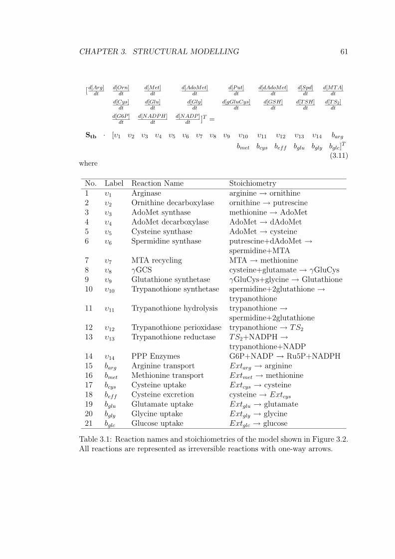
CHAPTER 4. INITIAL KINETIC MODEL 115
putrescine was found to drop to 40% of the normal value. The kinetic mechanism
of the enzyme is modelled in equation (4.16).
dAdoMet is present in parasites with a low intracellular concentration (Yarlett
et al. 1993). Methylthioadenosine (MTA) is the second product formed during
the transfer of an aminopropyl group from dAdoMet to putrescine. MTA is not
detectable in mammals because of its rapid degradation rate (Rodriguez-Caso
et al. 2006). In T. brucei, MTA is rapidly consumed by MTA phosphorylase to
adenine and 5’-methylthioribose-1-phosphate, where the latter is then converted
back to methionine (Berger et al. 1996) (More details can be found later in this
chapter). Owing to the rapid metabolization of MTA, the intracellular concen-
tration of this compound is low (Peter S. Backlund et al. 1982). Spermidine,
however, is present in millimolar concentrations. The spermidine-putrescine ra-
tio of intracellular concentrations in T. brucei was given in the range of 2:1
(Taylor et al. 2008) or 19:1 (Bacchi et al. 1977) in different studies.
A mathematical rate expression for SpdS is modelled in the form
VSpdS = V SpdSmax ·
[dAdoMet]
KSpdSmdAdoMet
1 +[dAdoMet]
KSpdSmdAdoMet
+[MTA]
KSpdSiMTA
·[Put]
KSpdSmP
1 +[Put]
KSpdSmP
+[Spd]
KSpdSiD
(4.16)
where V SpdSmax is the maximum velocity of SpdS. KSpdS
mdAdoMet and KSpdSmP repre-
sent half-saturation constant to substrate dAdoMet and putrescine. KSpdSiD and
KSpdSiMTA are the constants of competitive inhibition by spermidine (Spd) and
MTA, respectively.
Table 4.5 contains parameter values for T. brucei SpdS.
Enzyme involved in methionine recycling from MTA MTA, the byprod-
uct of aminopropyl group transfer from dAdoMet, is recycled to methionine via
a series of enzymatic steps in trypanosomes (Sufrin et al. 2008). The MTA recy-
cling path has been illustrated in mammals (Peter S. Backlund and Smith 1981),
and also observed in parasitic protozoa (Berger et al. 1996, Reguera et al. 2007).
MTA is first converted to methylthioribose-1-phosphate by MTA phosphory-
lase; the latter product is then metabolized to keto-methylthiobutyrate, which
is finally transaminated to methionine.
Methionine has a unique role in cellular growth, originating in its metabolic
conversion to AdoMet, which then participates in several downstream pathways

CHAPTER 4. INITIAL KINETIC MODEL 116
Parameters Description Value/Ranges SourceV SpdS
max maximum 0.0119μmol/mg/min (Taylor et al. 2008)velocity
KSpdSmdAdoMet half-saturation 0.09±0.01 μM (Taylor et al. 2008)
constant (Bitonti et al. 1984)
KSpdSmP half-saturation 205±65 μM (Taylor et al. 2008)
constant (Bitonti et al. 1984)
KSpdSiD inhibition 100 μM (Taylor et al. 2008)
constant
KSpdSiMTA inhibition 1–1000 μM Modelling
constant Assumption
Table 4.5: Parameter values for T. brucei SpdS.
of polyamine biosynthesis and methylation reactions. A constant supply of me-
thionine is imperative for cell proliferation, which requires adequate AdoMet in
physiological functions. The amount of methionine in the environment is lim-
ited and de novo synthesis is energetically expensive (Riscoe et al. 1989). MTA
recycling therefore seems to be an important source of this amino acid.
Because of the importance of MTA recycling in retaining cell viability, in-
terference with methionine metabolism has been explored as a potential target
for chemotherapy for African trypanosomiasis (Porter and Sufrin 1986, Bacchi
et al. 1991, Riscoe et al. 1989, Sufrin et al. 1995).
It has been established that methionine is regenerated via a multistep metabo-
lism of MTA, kinetics for which, however, are not available experimentally.
Available quantitative descriptions for the recycling path limit to the half-
saturation constant of MTA phosphorylase with respect to its substrate MTA.
Since the enzyme has a broad substrate specificity (Ghoda et al. 1988), the in
vivo maximum velocity is hard to obtain, but it is assumed to hold a very high
value (Bacchi et al. 1991).
MTA degradation is important; its accumulation is potentially toxic to mam-
malian cells (Christa et al. 1988). MTA can be degraded through normal protein
efflux or utilization in the recycling path. In our study, we consider methionine
regeneration as the major route of MTA consumption, which is assumed to oc-
cur via a single-step reaction. ‘MetRcy’ is used to denote the enzyme catalyzing
this reaction. Standard Michaelis-Menten kinetics are applied to describe the
CHAPTER 4. INITIAL KINETIC MODEL 117
enzyme kinetics, shown below:
VMetRcy = V MetRcymax ·
[MTA]
KMetRcymMTA
1 +[MTA]
KMetRcymMTA
(4.17)
where V MetRcymax and KMetRcy
mMTA are the maximum velocity of the enzyme and half-
saturation constant to substrate MTA.
Table 4.6 contains parameter values for T. brucei MetRcy catalyzing the
methionine regeneration from MTA.
Parameters Description Value/Ranges SourceV MetRcy
max maximum 1–50 μmol/min/mg Modelling Assumptionvelocity
KMetRcymMTA half-saturation 1–1000 μM Modelling Assumption
constant
Table 4.6: Parameter values for the enzyme on the methionine recycling path inT. brucei.
Trans-methylation Processes AdoMet is the common substrate for both
transmethylation processes and polyamine biosynthesis. The byproduct of AdoMet
methyl donation is S-adenosylhomocysteine (AdoHcy). AdoHcy is then cleaved
to salvage adenosine and homocysteine, where the latter is consumed by trans-
sulfuration events to produce cystathionine and cysteine (Bacchi et al. 1995).
Enzymes of MAT, AdoHcy hydrolase, homocysteine methyltransferase and
AdoMet transmethylases have been detected in cell-free extracts of T. brucei
(Yarlett and Bacchi 1988). AdoHcy exerts a feedback inhibition on AdoMet in
most methylation reactions (Chiang et al. 1996). In T. brucei, transmethylation
reactions were found to be very sensitive to AdoHcy inhibition with an apparent
KI value of 12.9 μM (Yarlett et al. 1991).
By contrast, in mammalian cells, homocysteine is recycled to methionine via
enzymatic catalysis by BHMT4 or MTR5 (Sufrin et al. 1995). Parasitic T. cruzi
and Leishmania species lack the enzyme methionine synthase, which catalyses
the methionine production from homocysteine (Reguera et al. 2007). However,
4Systematic name: Betaine-homocysteine methyltransferase5Systematic name: 5-methyltetrahydrofolate-homocysteine methyltransferase

CHAPTER 4. INITIAL KINETIC MODEL 118
debate remains as to whether homocysteine can be converted to methionine
in T. brucei. It was speculated that whether homocysteine is remethylated
to methionine or irreversibly committed to tran-ssulfuration, largely depends
on AdoMet concentration (Yarlett and Bacchi 1988). A different argument by
Goldberg et al. (Goldberg et al. 2000) suggested that, even though homocysteine
remethylation may exist in T. brucei, as most trans-sulfuration metabolites are
excreted from trypanosomes, any homocysteine recycled to methionine was not
as significant as methionine regeneration from MTA. In the current stage of
model construction, we consider the MTA recycling path as the unique source
of methionine reproduction.
Yarlett and Bacchi (Yarlett and Bacchi 1988) observed that, in contrast to
an enormous elevation of AdoMet level, AdoHcy remained undetectable in T.
brucei after 12hrs and 36hrs of DFMO treatment . This could be explained with
the high activity of cystathionine synthase in T. brucei that effectively converts
AdoHcy into cystathionine and cysteine.
The ratio of AdoMet to AdoHcy, termed the ‘Methylation index’ indicates
the transmethylation potential of a cell. Normal methylation index values were
shown to range from 2:1 to 9:1 (Bacchi et al. 1995). The ratio increased al-
most 20 fold in DFMO-treated trypansomes compared to the ratio under nor-
mal conditions from 6.5 to 114 after 24 hours of DFMO treatment (Yarlett and
Bacchi 1988). Under normal conditions, a decline of the ratio, resulting from
either a reduction in AdoMet or an accumulation of AdoHcy, can induce the
so-called hypermethylation status leading to cell death (Reguera et al. 2007).
Bloodstream-form trypanosomes undergo significant changes in cell methy-
lation events in response to the intervention of polyamine synthesis. Under per-
turbed conditions, the levels of transmethylation byproducts, cystathionine and
cysteine can be rapidly increased. In DFMO-treated trypanosomes, cysteine
and cysthationine in the incubation medium, increased about 5-fold (Bacchi
et al. 1995), while the intracellular pools did not vary significantly from the con-
trol cells. A substantial flow from AdoMet through AdoHcy was also observed,
indicating that the rate of AdoMet utilization in trans-methylation processes
under DFMO treatment may be several times higher than that in normal con-
ditions.
In our study, the consideration of trans-methylation processes is limited to
the first step describing the conversion of AdoMet into AdoHcy. The remaining
reactions under the catalysis of a number of enzymes, including AdoHcy hy-

CHAPTER 4. INITIAL KINETIC MODEL 119
drolase, cystathionine syntase and cystathionase, are excluded from the model,
partially because no or very limited kinetic information is available for the en-
zymes. More importantly, under the DFMO-induced condition, the intermedi-
ates of tran-smethylation processes were quickly excreted into the environment,
and no significant changes were observed in intracellular concentrations of the
metabolites (Bacchi et al. 1995, Yarlett and Bacchi 1988).
Since the kinetic modelling is primarily concerned with evaluating the try-
panothione metabolism under the treatment of anti-trypanosomal drug DFMO,
the trans-methylation intermediates that have no or negligible effects on the in-
tended use of the model are not included. AdoHcy production is incorporated
in the model for its potential role in adjusting the intracellular AdoMet concen-
tration, where the latter is a critical metabolite for trypanothione biosynthesis.
AdoHcy is regarded as a constant metabolite during the in silico simulation and
the methylation index 2:1 is assumed for the ratio of AdoMet to AdoHcy at
normal conditions (resulting in the constraint [AdoHcy] = 0.5 · [AdoMet]) to
approximate the relationship between the concentrations of the metabolites.
‘AHS’ is used to denote the enzyme catalyzing the AdoHcy production from
AdoMet. The kinetic mechanism of the enzyme is modelled based on the stan-
dard Michaelis-Menten kinetics
VAHS = V AHSmax ·
[AdoMet]
KAHSmAdoMet
1 +[AdoMet]
KAHSmAdoMet
+[AdoHcy]
KAHSiAdoHcy
(4.18)
where V AHSmax and KAHS
mAdoMet are the maximum velocity and half-saturation con-
stant to substrate AdoMet. KAHSiAdoHcy is the constant of competitive inhibition
by AdoHcy.
Table 4.7 contains parameter values for T. brucei AHS catalyzing the chem-
ical conversion from AdoMet to AdoHcy.
Methionine & Arginine Transport The uptake rate V MetPtmax of exogenous
methionine into the cytosol of T. brucei was measured to be 8.9×10⁻⁷ mol/L/min
at 26 μM, the human serum concentration of methionine (Goldberg et al. 2000).
Different kinetics were reported by Hasne and Barrett (Hasne and Barrett 2000)
as V MetPtmax = 28.8±0.1 nmol ·min−1 ·(108 cells)−1 and KMetPt
m = 32.8±3.4 μM. In
our study, the numbers from Hasne and Barrett are used for its known validity.

CHAPTER 4. INITIAL KINETIC MODEL 120
Parameters Description Value/Ranges SourceV AHS
max maximum 1e-3–50 μmol/min/mg Modellingvelocity Assumption
KAHSmAdoMet half-saturation 1–1000 μM Modelling
constant AssumptionKAHS
iAdoHcy inhibition 12.9 μM (Yarlett et al. 1991)constant
Table 4.7: Parameter values for the enzyme of AdoHcy production in T. brucei.
Kinetics of exogenous methionine uptake are modelled as a standard Michaelis
Menten, given below:
VMetPt = V MetPtmax ·
[Met]exg
KMetPtm
1 +[Met]exg
KMetPtm
(4.19)
where [Met]exg is the exogenous methionine concentration (26 μM). V Metmax and
KMetPtm are the maximum velocity and the half-saturation constant with respect
to the substrate.
To express the maximum velocity in μmol min−1 (mg cell protein)−1, an
assumption that transporter enzymes account for 10% of overall cell protein
of trypanosome is applied (refer to Section 3.5.1 for detailes). This gave the
maximum velocity of the transporter enzyme of exogenous methionine a value
of 0.276 μmol min−1 (mg cell protein)−1.
A biological experiment examining exogenous arginine uptake was designed
for the task by the group of Mike Barrett. The experimental results showed
that exogenous arginine was taken into T. brucei through two transporters with
distinct affinities. Carriers were measured with a high capacity V ArgPtmaxH and a low
capability V ArgPtmaxL upto 0.9 μmol/min/mg and 0.14 μmol/min/mg, respectively;
half-saturation constants KArgPtmH , 1130 μM and KArgPt
mL , 26 μM, were measured
for each carrier. Exogenous arginine is considered as a constant supply into the
system; the concentration is assumed to be 33 μM in plasma. In accordance
with the experimental observations, arginine transport was expressed as the
superposition of transport functions via both carriers as follows
VArgPt = V ArgPtH + V ArgPt
L (4.20)
CHAPTER 4. INITIAL KINETIC MODEL 121
where
V ArgPtH = V ArgPt
maxH ·[Arg]exg
KArgPtmH
1 +[Arg]exg
KArgPtmH
(4.21)
V ArgPtL = V ArgPt
maxL ·[Arg]exg
KArgPtmL
1 +[Arg]exg
KArgPtmL
(4.22)
The aforementioned biological experiment indicated that in T. brucei argi-
nine has a much lower uptake capability compared to methionine. In Chapter 3
we highlighted that arginine transport observed in L. donovani is about 30 times
higher than the number measured in T. brucei. Even at the level observed in
L. donovani, arginine transport is still not comparable to methionine transport.
Due to the large uncertainty in the numbers reported for arginine transport in
T. brucei, we choose to treat them as unknown parameters. This results in the
following kinetic equation, which replaces the preceding set of equations.
VArgPt = V ArgPtmax ·
[Arg]exg
KArgPtm
1 +[Arg]exg
KArgPtm
(4.23)
where [Arg]exg is the exogenous arginine concentration (30 μM). V ArgPtmax and
KArgPtm are the maximum velocity and half-saturation constant with respect to
exogenous arginine. They are expressed in μmol per min per mg of cell protein
and μM, and constrained by the boundary conditions 0 < V ArgPtmax ≤ 1 and
1 ≤ KArgPtm ≤ 1000, respectively. These unknown parameters will be estimated
during the in silico simulation.
4.3.2 Glutathione Biosynthesis
Glutathione biosynthesis in the model starts from cysteine, to which bloodstream-
form T. brucei is very sensitive. Cysteine in human serum has concentration of
13 μM and can be effectively incorporated into the cell with the maximum veloc-
ity and half-saturation constant at 0.3 μmol ·min−1 ·(mg cell protein)−1 and 400
μM (Duszenko et al. 1985). Cysteine transport is modelled with the standard

CHAPTER 4. INITIAL KINETIC MODEL 122
Michaelis-Menten kinetic, as below:
VCysPt = V CysPtmax ·
[Cys]exg
KCysPtm
1 +[Cys]exg
KCysPtm
(4.24)
where [Cys]exg stands for the concentration of exogenous cysteine. V CysPtmax and
KCysPtm are the maximum velocity and half-saturation constant with respect to
exogenous cysteine.
Conversion of cysteine into glutathione occurs as a two-step enzymatic re-
action. The first and rate-limiting step in the biosynthesis of glutathione is the
ligation of glutamate (Glu) and cysteine (Cys), catalyzed by γ-glutamylcysteine
synthase (gGCS); the product L-γ-glutamyl-L-cysteine (gGluCys) is then con-
verted to glutathione by glutathione synthase (GS) through addition of glycine
(Gly). Huynh et al. (Huynh et al. 2003) observed that gGCS is an essential
enzyme for the growth of T. brucei cells, implying gGCS as a potential drug
target.
Enzyme γGCS is modelled in the form:
VgGCS = V gGCSmax ·
[Glu]
KgGCSmGlu
1 +[Glu]
KgGCSmGlu
+[GSH]
KgGCSiGSH
·
[Cys]
KgGCSmCys
1 +[Cys]
KgGCSmCys
·[ATP ]
KgGCSmATP
1 +[ATP ]
KgGCSmATP
(4.25)
where [Glu] and [Cys] represent the concentrations of the co-substrates of the
enzyme. [ATP ] represents the concentration of a cofactor of the reaction, where
the value is reported in Table 4.3. V gGCSmax is the maximum velocity of the enzyme.
KgGCSmGlu , KgGCS
mCys and KgGCSmATP are the half-saturation constants for each reactant of
the reaction. KgGCSiGSH stands for the feedback inhibition from product glutathione,
which is competitive with respect to the co-substrate glutamate.
Table 4.8 contains parameters for T. brucei gGCS.
GS was only measured in Plasmodium falciparum (Meierjohann et al. 2002)
and no information is available for the enzyme in T. brucei. In our analysis,

CHAPTER 4. INITIAL KINETIC MODEL 123
Parameters Description Value/Ranges SourceV gGCS
max maximum 7.6 μmol/min/mg (Lueder and Phillips 1996)velocity
KgGCSmGlu half-saturation 240 μM (Lueder and Phillips 1996)
constant
KgGCSmCys half-saturation 690 μM (Lueder and Phillips 1996)
constant
KgGCSmATP half-saturation 70 μM (Lueder and Phillips 1996)
constant
KgGCSiGSH feedback 1100 μM (Lueder and Phillips 1996)
inhibition[Glu] intracellular 3000 μM Experimental Data
concentration from Mike Barrett
Table 4.8: Parameter values for T. brucei γGCS.
kinetics of GS are modelled with the standard Michaelis-Menten law:
VGS = V GSmax ·
[Gly]
KGSmGly
1 +[Gly]
KGSmGly
·[ATP ]
KGSmATP
1 +[ATP ]
KGSmATP
·[gGluCys]
KGSmgGluCys
1 +[gGluCys]
KGSmgGluCys
(4.26)
where V GSmax is the maximum velocity. KGS
mGly, KGSmgGluCys and KGS
mATP repre-
sent the half-saturation constants of the enzyme with respect to the substrates
glycine, gGluCys and ATP, respectively.
Table 4.9 contains parameters for T. brucei GS.
Parameters Description Value/Ranges SourceV GS
max maximum 1e-3–20 μmol/min/mg Modellingvelocity Assumption
KGSmGly half-saturation 1–1000 μM Modelling
constant AssumptionKGS
mATP half-saturation 1–1000 μM Modellingconstant Assumption
KGSmgGluCys half-saturation 1–1000 μM Modelling
constant Assumption[Gly] intracellular 4000 μM Experimental Data
concentration from Mike Barrett
Table 4.9: Parameter values for T. brucei GS.

CHAPTER 4. INITIAL KINETIC MODEL 124
The Reversible Reaction of Trypanothione Production
The biosynthetic reaction of trypanothione consists of two steps. First, two
molecules of spermidine are combined with glutathione to synthesize a glutathione-
spermidine dithiol conjugate (GspdSH) that plays a central role in several detox-
ification processes, which is followed by the formation of trypanothione from
the conjugate and one molecule of glutathione. The enzymes of trypanothione
biosynthesis are potential targets for drug design.
TryS: Trypanothione Synthetase Trypanothione synthetase has been the
focus of anti-trypanosomal research, owing to not only its significant role in
trypanosomal viability but also its capability in regulating the levels of GspdSH,
spermidine and glutathione.
Recent work (Willert and Phillips 2008) discovered that, the absence of
GspdSH or trypanothione led to trypanosome death. Willert and Phillips ob-
served that trypanosome death followed an irreversible process. This implies that
when the intracellular spermidine level is lower than a physiologically required
level, the biosynthesis of GspdSH or trypanothione cannot be hardly fulfilled.
The authors suggested that the cell did not build up GspdSH and trypanothione
pools until spermidine level reached an appropriate steady-state set point. This
is commonly referred to as the homeostasis response, a so-called ultrasensitive
response to external signals.
Both a synthetase and amidase activity has been associated with glutathionyl-
spermidine synthetase in Escherichia coli (Kwon et al. 1997, Bollinger et al.
1995), and trypanothione synthetase in Leishmania parasites (Fyfe et al. 2008),
Crithidia fasciculata (Oza et al. 2002) and T. brucei (Oza et al. 2003). The
conflicting activities of synthetase and amidase, which allow for a bidirectional
response between the involved metabolites, may serve to modulate intracellular
levels of the metabolites without additional protein synthesis or degradation of
existing metabolites.
The regulation mechanism between synthetase and amidase is not yet pre-
cisely characterized in T. brucei. However, some qualitative properties of this
enzyme can be predicted by studying other organisms. For example, under nor-
mal conditions, in Escherichia coli, the activity of the amidase site is about
40-fold lower than that of the synthetase site and the former prefers GspdSH as
a substrate over trypanothoine for effective hydrolysis.
Fyfe et al. (Fyfe et al. 2008) observed that the structure of L. major trypan-

CHAPTER 4. INITIAL KINETIC MODEL 125
othione synthetase-amidase has two active sites, where each site binds to differ-
ent molecules for specific functions. Due to the substantial amount of similarity
shared by parasitic Leishmania and Trypanosoma species, it is assumed that
there are no interactions between the active sites of T. brucei synthetase-amidase
and the kinetic behaviour of the conflicting activities are modelled separately.
Kinetic mechanisms of the synthetase catalyzing GspdSH and trypanothione
production are given in equations (4.28) and (4.27), and the amidase kinetics
responsible for the hydrolysis of trypanothione and GspdSH in equations (4.29)
and (4.30), respectively. Parameters for trypanothione synthetase (TryS) and
admidase (TryAdm) are contained in Table 4.10.
V gdTryS =
KTryScat · [TryS]
1 +KTryS
mGSH
[GSH]+
[GSH]
KTrySsiGSH
·[ATP ]
KTrySmATP
1 +[ATP ]
KTrySmATP
· (4.27)
([Spd]
KTrySmD
)n
1 +
([Spd]
KTrySmD
)n
+[GspdSH]
KTrySmGspdSH
V ggTryS =
KTryScat · [TryS]
1 +KTryS
mGSH
[GSH]+
[GSH]
KTrySsiGSH
·
[GspdSH]
KTrySmGspdSH
1 +[GspdSH]
KTrySmGspdSH
·[ATP ]
KTrySmATP
1 +[ATP ]
KTrySmATP
(4.28)
V TSHTryAdm = V TryAdm
maxTSH ·[TSH]
KTryAdmmTSH
1 +[TSH]
KTryAdmmTSH
(4.29)
V GspdSHTryAdm = V TryAdm
maxGspdSH ·
[GspdSH]
KTryAdmmGspdSH
1 +[GspdSH]
KTryAdmmGspdSH
(4.30)

CHAPTER 4. INITIAL KINETIC MODEL 126
Parameters Description Value/Ranges Source
kTryScat turn-over rate 2.9±0.4 s−1 (Oza et al. 2003)
KTrySmGspdSH half-saturation 2.4 μM (Oza et al. 2003)
constant
KTrySmGSH half-saturation 56.2 μM (Oza et al. 2003)
constant
KTrySmATP half-saturation 7.1 μM (Oza et al. 2003)
constant
KTrySmD half-saturation 37.8 μM (Oza et al. 2003)
constant
V TryAdmmaxTSH maximum 6.4e-3 μmol/min/mg (Oza et al. 2003)
velocity
KTryAdmmTSH half-saturation 1–1000 μM Modelling
constant Assumption
V TryAdmmaxGspdSH maximum 21e-3 μmol/min/mg (Oza et al. 2003)
velocity
KTryAdmmGspdSH half-saturation 1–1000 μM Modelling
constant Assumption
KTrySsiGSH substrate 36.5 μM (Oza et al. 2003)
inhibitionn hill coefficient 1–3 Modelling
Assumption[TryS] enzyme 1e-5–0.5 μM Modelling
concentration Assumption
Table 4.10: Parameter values for T. brucei TryS and TryAdm.
where kTryScat is the turnover number. KTryS
mGspdSH , KTrySmGSH , KTryS
mD and KTrySmATP
represent the half-saturation constants of TryS with respect to the substrates
GspdSH, glutathione and spermidine and co-factor ATP, respectively. n rep-
resents the hill coefficient that substrate spermidine may exercise on the en-
zyme. KTrySsiGSH is the substrate inhibition coefficient of glutathione. V TryAdm
maxTSH ,
V TryAdmmaxGspdSH and KTryAdm
mTSH , KTryAdmmGspdSH stand for the maximum velocity and half-
saturation constants of enzyme TryAdm with respect to the substrates TSH and
GspdSH, respectively.
Table 4.10 contains parameters for T. brucei TryS and TryAdm.

CHAPTER 4. INITIAL KINETIC MODEL 127
4.3.3 Trypanothione Oxidation and Regeneration
In most eukaryotes, the glutathione peroxidase-glutathione reductase system
protects cells against oxidative stress. In trypanosomes, the defense mechanism
against oxidative stress is instead achieved by the cyclic action of trypanothione
and the enzymes trypanothione peroxidase and trypanothione reductase.
TPx: Trypanothione Peroxidase Oxidative stress, represented as the level
of hydrogen peroxide (H2O2), is toxic to parasites, which is produced from molec-
ular oxygen in the living environment of parasites. Under normal conditions,
H2O2 is maintained at very low intracellular concentrations by various enzymes
and molecular antioxidants. An intracellular concentration of 0.1 μM is assumed
in our analysis. H2O2 can be consumed by either glutathione or trypanothione
as substrate via both enzymatic and non-enzymatic reactions.
The non-enzymatic processes are excluded from the model, since the non-
enzymatic reduction of H2O2 accounts for only a small proportion of the overall
H2O2 consumption (Henderson et al. 1987). The major route of H2O2 con-
sumption is through the fast response of trypanothione under the catalysis of
trypanosome peroxidase, as shown in reaction (4.31). Trypanosomes can convert
one molecule of H2O2 to two molecules of H2O using trypanothione which is ox-
idized to form trypanothione disulfide (TS2) in the process. TS2 then rapidly
reacts with NADPH to regenerate the intracellular pool of trypanothione. T.
brucei was found to have a value of 1.3 nmol · min−1 · (108 cells)−1 for trypan-
othione peroxidase when using H2O2 as an oxidant (Penketh and Klein 1986).
T (SH)2 + H2O2 −→ TS2 + 2H2O : TPx (4.31)
The standard Michaelis-Menten kinetics are applied to TPx, shown below:
VTPx = V TPxmax ·
[TSH]
KTPxmTSH
1 +[TSH]
KTPxmTSH
·[H2O2]
KTPxmH2O2
1 +[H2O2]
KTPxmH2O2
(4.32)
where V TPxmax is the maximum velocity of enzyme TPx. KTPx
mTSH and KTPxmH2O2
are
the half-saturation constants of TPx with respect to the substrates TSH and
H2O2, respectively.
Trypanothione peroxidase has a very low half-saturation constant with re-

CHAPTER 4. INITIAL KINETIC MODEL 128
spect to substrate H2O2, and is assumed to have a value of 1 μM in our analysis
(Henderson et al. 1987, Penketh and Klein 1986). The half-saturation constant
KTPxmTSH is an unknown parameter. A range of 1–1000 (μM) is given to this
parameter.
H2O2 production in T. brucei has been determined to fall somewhere in the
range 0.2–0.7 nmol · min−1 · (108 cells)−1 (Henderson et al. 1987, Penketh and
Klein 1986). The dynamics of H2O2 are modelled in the form of the difference
between the production rate and consumption rate as follows
d[H2O2]
dt= RH2O2
g − VTPx (4.33)
where RH2O2g represents H2O2 generation in bloodstream-form T. brucei.
TR: Trypanothione Reductase Trypanothione reductase serves an impor-
tant role in the regulation of the intracellular thiol-redox balance and in defense
against oxidant.
It catalyses the conversion of TS2 into trypanothione and trypanosomes with
reduced TR levels were found to be very vulnerable to oxidative stress (Krieger
et al. 2000, Khan 2007). Kinetics for TR are only available for T. cruzi; however
these values are included in the model of T. brucei due to the similarity shared
by the two organisms. The standard Michaelis-Menten law is applied to describe
the kinetic mechanism of TR.
VTR = V TRmax ·
[NADPH]
KTRmNADPH
1 +[NADPH]
KTRmNADPH
·[TS2]
KTRmTS2
1 +[TS2]
KTRmTS2
(4.34)
where V TRmax is the maximum velocity and KTR
mTS2and KTR
mNADPH stand for the
half-saturation constants with respect to the substrate TS2 and coenzyme NADPH.
Table 4.11 contains parameters for T. brucei TR.
Contradicting Observations on Glutathione Reductase The removal of
H2O2 through the action of glutathione peroxidase and glutathione reductase
in mammalian cells is replaced in T. brucei by trypanothione acting as a redox
carrier. It is commonly recognized that T. brucei does not contain glutathione
peroxidase, but a conflicting observation was reported regarding the presence of

CHAPTER 4. INITIAL KINETIC MODEL 129
Parameters Description Value/Ranges SourceV TR
max maximum 112.7 μmol/min/mg (Krauth-Siegel et al. 1987)velocity
KTRmTS2
half-saturation 9 μM (Krauth-Siegel et al. 1987)constant
KTRmNADPH half-saturation 36 μM (Krauth-Siegel et al. 1987)
constant
Table 4.11: Parameter values for T. brucei TR. Note that the values are obtainedfrom experiments on T. cruzi.
glutathione reductase (GR) in the organism. Krauth-Siegel and Comini (Krauth-
Siegel and Comini 2008) observed that T. brucei lacks the necessary genes for
glutathione reductase. However, Fairlamb and Cerami (Fairlamb et al. 1985)
indicate that the activity of glutathione reductase could be readily measured in
the presence of the co-factor trypanothione, and the enzyme-mediated reaction
can be written as follows
GSSG + NADPH −→ 2GSH + NADP : GR (4.35)
GSSG is toxic to cells and under normal conditions it does not accumu-
late because it reduces to glutathione. The rate equation of the enzyme GR
is modelled below. The maximum velocity of GR was reported as 1.4 nmol ·min−1 · (108 cells)−1 (Penketh and Klein 1986) or 4.5 nmol ·min−1 · (108 cells)−1
(Fairlamb et al. 1985).
VGR = V GRmax ·
[GSSG]
KGRmGSSG
1 +[GSSG]
KGSSGmGSSG
·[NADPH]
KGRmNADPH
1 +[NADPH]
KGRmNADPH
(4.36)
where V GRmax is the maximum velocity and KGR
mGSSG and KGRmNADPH stand for the
half-saturation constants with respect to the substrate GSSG and co-enzyme
NADPH.
In T. brucei, trypanothione is a spontaneous reductant of GSSG and thiore-
doxin (Krauth-Siegel et al. 2005). In the present kinetic model, the involvement
of trypanothione in the consumption of GSSG and thioredoxin is neglected owing
to its instantaneous occurrence. The enzymatic reaction in which trypanothione
metabolizes H2O2 is taken as the only reaction that trypanothione participates

CHAPTER 4. INITIAL KINETIC MODEL 130
in as a substrate. Moreover, because of the contradicting observations reported
for GR, the rate equation (4.36) is not taken into account in the modelling pro-
cess. Further clarification is required regarding the presence of this enzyme and
its associated kinetics.
4.3.4 Formation of NADPH and Pentoses
Glycolysis in bloodstream-form T. brucei cells provides a convenient context for
studying the enzyme inhibitors to be used as anti-parasitic drugs (Eisenthal and
Cornish-Bowden 1998) because of the significant differences in the organization
of glycolysis in parasites and host cells. The model of trypanosomal glycolysis
developed by Bakker et al. (Bakker et al. 1997) provides a good starting point
for a systematic investigation of potential drug targets.
Glycolysis represents the sole pathway for glucose metabolism to provide cells
with energy ATP, and bloodstream-form T. brucei depends completely on rapid
glycolysis for its energy supply. Glucose metabolism is facilitated by the glucose
transporter of T. brucei, which follows a reversible process. Intracellular glucose
is converted into D-glucose 6-phosphate (G6P) under the catalysis of hexokinase
(HKK), and consequently glycerol and ribose. The majority of intermediate
compounds and enzymes of the glycolysis pathway are located in the glycosome
of T. brucei.
The pentose phosphate pathway plays a crucial role in the metabolism of
many parasitic protozoa and in the host-parasite relationship (Barrett et al.
2003). The pathway maintains intracellular pools of NADP and NADPH, where
the latter is used as substrate in the protection of trypanosomes against oxida-
tive stress. The cellular ratio of NADPH to NADP is an important means of
regulating the metabolic flux through the pathway. When the NADPH/NADP
ratio is high, a powerful inhibition of trypanosomal growth may occur.
The pentose phosphate pathway converts glucose 6-phosphate (G6P) to ri-
bose 5-phosphate (Ru5P) via a sequence of enzymatic reactions, and the ma-
jority of the pathway intermediates are shown to be cytosolic in T. brucei. The
enzyme hexokinase catalyzing the production of glycosomal G6P is reported to
have an exclusively glycosomal location and T. brucei has not been evidenced to
be able to synthesize G6P de novo in cytosol. This compartmentation constraint
leads to a question of where the required metabolites of the pentose phosphate
pathway come from, especially in the case of G6P. One theory is that a trans-

CHAPTER 4. INITIAL KINETIC MODEL 131
porter exists in the glycosomal membrane that facilitates the transfer of this
intermediate between the glycosome and cytosol (Barrett 1997). However, no
kinetic information describing this postulated membrane transporter in T. bru-
cei has ever been reported. To enable the in silico simulation, we assume that
G6P concentrations in the glycosome and the cytosol are equal, and thus the
well-understood kinetics of glycosomal hexokinase can be applied to the present
model.
The complete pentose phosphate pathway consumes G6P to produce ri-
bose via a series of enzymatic reactions catalyzed by the enzymes Glucose-
6-phosphate Dehydrogenase (G6PDH), 6-phosphogluconolactonase (6PGL), 6-
phosphogluconate dehydrogenase (6PGDH), ribose 5-phosphate isomerase and
ribokinase, leading to the intermediate products D-glucono-1,5-lactone 6-phosph-
ate (6-PGL), 6-phospho-D-gluconate (6-PG), D-ribulose 5-phosphate (Ru5P), D-
ribose 5-phosphate (R5P) and ribose, respectively. In the present kinetic model,
the pentose phosphate pathway is revised in accordance with the intended use
of the model. Two primary factors for trypanosomal growth – trypanothione
biosynthesis and oxidant detoxification – are the focus of the study of trypan-
othione metabolism. Owing to the critical role of NADPH in the defense mech-
anism against oxidative stress, the consideration of the pathway is limited to the
elementary steps that produce NADPH.
The pentose phosphate pathway can be separated into an oxidative branch
and a non-oxidative branch. The oxidative branch of the pathway involves
G6PDH, 6PGL and 6PGDH, which are essential for the protection of the par-
asite against oxidative stress. The reactions processing the exchange between
NADP and NADPH are the reactions catalyzed by G6PDH and 6PGDH, given
as follows
G6P + NADP −→ 6-PGL + NADPH : G6PDH (4.37)
6PG + NADP −→ Ru5P + NADPH : 6PGDH (4.38)
The intermediate reaction responsible for the production of 6PG (the reac-
tant in the chemical reaction in equation (4.38)), occurs spontaneously compared
to other enzymatic reactions in the pathway. 6PGL is a unstable compound
and the necessity of 6PGL to catalyze this reaction in the cells is questionable
(Duffieux et al. 2000). For this reason, a direct conversion from 6PGL into Ru5P
is assumed. Combined with the aforementioned reactions for glucose transport

CHAPTER 4. INITIAL KINETIC MODEL 132
and glycosomal G6P production, the revised pentose phosphate pathway is rep-
resented by the following chemical reactions:
Glucoseext ←→ Glucoseg : GlcPt (4.39)
Glucoseg + ATP −→ G6P + ADP : HKK (4.40)
G6P + NADP −→ 6PG + NADPH : G6PDH (4.41)
6PG + NADP −→ Ru5P + NADPH : 6PGDH (4.42)
Kinetic mechanisms of the required enzymes catalyzing the above reactions
are documented in the following paragraphs.
GlcPt: Glucose Transport The kinetics of glucose transport are known in
detail. We apply the kinetic equation defined by Haanstra et al. (Haanstra
et al. 2008) to model the dynamics of glucose transport, shown below:
VGlcP t = V GlcP tmax · [Glc]ext − [Glc]g
KGlcP tm + [Glc]ext + [Glc]g + α · [Glc]ext
[Glc]gKGlcP t
m
(4.43)
where V GlcP tmax is the maximum velocity of the forward glucose transport reaction.
[Glc]ext and [Glc]g represent the concentrations of exogenous and glycosomal
glucose. As glucose transport is modelled as a reversible reaction, KGlcP tm is thus
the generalized half-saturation constant. α is the scaling factor adjusting the
weight of the forward glucose uptake and the backward glucose efflux.
Table 4.12 contains parameters for T. brucei glucose transport.
Parameters Description Value/Ranges SourceV GlcP t
max maximum 0.109 μmol/min/mg (Haanstra et al. 2008)velocity
KGlcP tm half-saturation 1000 μM (Haanstra et al. 2008)
constantα scaling factor 0.75 μM (Haanstra et al. 2008)[Glc]ext concentration 5000 μM (Haanstra et al. 2008)
in blood
Table 4.12: Parameter values for T. brucei glucose transport.

CHAPTER 4. INITIAL KINETIC MODEL 133
HXK: Hexokinase The kinetic equation of Hexokinase from the model of
glycolysis designed by Haanstra et al. (Haanstra et al. 2008) is adopted, which
is expressed as follows
VHKK = V HXKmax ·
[Glc]gKHXK
mGlcg
· [ATP ]gKHXK
mATP(1 +
[ATP ]gKHXK
mATP
+[ADP ]gKHXK
mADP
)·(
1 +[Glc]gKHXK
mGlcg
+[G6P ]
KHXKmG6P
) (4.44)
where V HXKmax is the maximum velocity. KHXK
mGlcgand KHXK
mATP are the half-saturation
constants of the enzyme with respect to endogenous glucose and co-factor ATP
in glycosome. KHXKmADP and KHXK
mG6P represent the inhibition constant of the prod-
ucts ADP and G6P, respectively.
Table 4.13 contains parameters for T. brucei HXK.
Parameters Description Value/Ranges SourceV HXK
max maximum 1.93 μmol/min/mg (Haanstra et al. 2008)velocity
KHXKmGlcg
half-saturation 100 μM (Haanstra et al. 2008)
constantKHXK
mATP half-saturation 116 μM (Haanstra et al. 2008)constant
KHXKmADP inhibition 126 μM (Haanstra et al. 2008)
constantKHXK
mG6P inhibition 12000 μM (Haanstra et al. 2008)constant
[ATP ]g concentration 240.5 μM (Haanstra et al. 2008)in glycosome
[ADP ]g concentration 1519 μM (Haanstra et al. 2008)in glycosome
Table 4.13: Parameter values for T. brucei HXK.
G6PDH: Glucose-6-phosphate Dehydrogenase G6PDH is the first en-
zyme of the pentose phosphate pathway. The product of the enzyme-mediated
reaction, G6P, is toxic to trypanosomes when it is accumulated. Several stud-
ies on T. brucei G6PDH however return us again to the fact that different
groups frequently present conflicting observations of enzyme activity. Cronin
et al. (Cronin et al. 1989) detected a maximum velocity of 0.0168±0.0057

CHAPTER 4. INITIAL KINETIC MODEL 134
μmol/min/mg and 0.0124±0.0038 μmol/min/mg for the bloodstream form and
procyclic form of T. brucei, respectively, whereas Heise and Opperdoes (Heise
and Opperdoes 1999) measured a maximum velocity of procyclic form T. bru-
cei G6PDH of 14μmol/min/mg. Duffieux et al. (Duffieux et al. 2000) however
reported a much higher value of 740 μmol/min/mg.
The maximum velocity of bloodstream-form T. brucei G6PDH is thus con-
sidered as an unknown parameter due to the conflicting data. The published in
vivo experiments were performed in a realistic environment, where the poten-
tial G6P transport between the glycosome and the cytosol are naturally taken
into account. However, in our kinetic model, no distinction was made between
glycosomal G6P and cytosolic G6P. Treating the maximum velocity of G6PDH
as an unknown parameter adds an extra degree of freedom to the system, which
allows the in silico model to be solved computationally.
Compared to the wide range of values reported for the specific activity of
G6PDH, there is less uncertainty about the value of half-saturation constants
of the enzyme with respect to the involved substrates. The half-saturation con-
stants are hence considered as known parameters, which are extracted from the
published articles.
The Michaelis-Menten based kinetics are applied to model the dynamics of
G6PDH, shown below:
VG6PDH = V G6PDHmax ·
[G6P ]
KG6PDHmG6P
1 +[G6P ]
KG6PDHmG6P
·[NADP ]
KG6PDHmNADP
1 +[NADP ]
KG6PDHmNADP
+[NADPH]
1 + [NADPH]
KG6PDHiNADPH
(4.45)
where V G6PDHmax is the maximum velocity. KG6PDH
mG6P and KG6PDHmNADP are the half-
saturation constants of G6PDH with respect to the substrate G6P and co-
enzyme NADP. KG6PDHiNADPH represents the inhibition constant of product NADPH
on the enzyme.
Table 4.14 contains parameters for T. brucei G6PDH.
Igoillo-Esteve et al. (Igoillo-Esteve et al. 2007) hypothesized that under
normal conditions, T. cruzi G6PDH is maintained in its reduced less-active form
by NADPH. Under oxidative stress, in which the level of the reduced cofactor
drops and other molecules like H2O2 are present, the enzyme is oxidized to attain
its more active form. This process would constitute a fast response to increase
NADPH level to counteract the oxidative stress.

CHAPTER 4. INITIAL KINETIC MODEL 135
Parameters Description Value/Ranges SourceV G6PDH
max maximum 1e-4–40 μmol/min/mg Modellingvelocity Assumption
KG6PDHmG6P half-saturation 138 μM (Duffieux et al. 2000)
constantKG6PDH
mNADP half-saturation 35 μM (Duffieux et al. 2000)constant
KG6PDHiNADPH inhibition 1–1000 μM Modelling
constant Assumption
Table 4.14: Parameter values for T. brucei G6PDH.
We propose that T. brucei G6PDH activity may also be induced by oxidative
stress due to the similarity shared by the two organisms. Accordingly, the rate
equation (4.45) is modified with the last factor representing the activation of
G6PDH by oxidative stress.
VG6PDH = V G6PDHmax ·
[G6P ]
KG6PDHmG6P
1 +[G6P ]
KG6PDHmG6P
·[NADP ]
KG6PDHmNADP
1 +[NADP ]
KG6PDHmNADP
+[NADPH]
1 + [NADPH]
KG6PDHiNADPH
· [H2O2] + Ka
[H2O2]ss + Ka
(4.46)
where [H2O2]ss and [H2O2] represent the concentration of H2O2 under steady-
state and oxidative stress conditions. Ka is the activation constant. When
[H2O2] = [H2O2]ss the factor is 1.
6PGDH: 6-phosphogluconate Dehydrogenase Hanau et al. (Hanau et al.
1996) performed detailed kinetic analysis of T. brucei 6PGDH. The authors
observed that NADPH acts as a competitive inhibitor of NADP and Ru5P is a
competitive inhibitor of 6PG. The maximum velocity of this enzyme has been
measured experimentally by Hanau et al.; however, this parameter is treated as
unknown in the present kinetic model for the same reasons as G6PDH.
The Michaelis-Menten based kinetics for 6PGDH dynamics are
V6PGDH = V 6PGDHmax ·
[6PG]
K6PGDHm6PG
1 +[6PG]
K6PGDHm6PG
+[Ru5P ]
K6PGDHiRu5P
·[NADP ]
K6PGDHmNADP
1 +[NADP ]
K6PGDHmNADP
+[NADPH]
K6PGDHiNADPH
(4.47)
where V 6PGDHmax is the maximum velocity. K6PGDH
m6PG and K6PGDHmNADP are the half-

CHAPTER 4. INITIAL KINETIC MODEL 136
saturation constants of 6PGDH with respect to the substrate 6PG and co-
enzyme NADP. K6PGDHiRu5P and K6PGDH
iNADPH represent the inhibition constants of
the products of the enzyme, Ru5P and NADPH, respectively.
Table 4.15 contains parameters for T. brucei 6PGDH.
Parameters Description Value/Ranges SourceV 6PGDH
max maximum 1e-4–40 μmol/min/mg Modellingvelocity Assumption
k6PGDHcat turnover 27 s−1 (Hanau et al. 1996)
numberK6PGDH
m6PG half-saturation 3.5 μM (Hanau et al. 1996)constant
K6PGDHmNADP half-saturation 1 μM (Hanau et al. 1996)
constantK6PGDH
iRu5P inhibition 30 μM (Hanau et al. 1996)constant
K6PGDHiNADPH inhibition 0.6 μM (Hanau et al. 1996)
constant[Ru5P ] intracellular 20 μM Modelling
concentration Assumption
Table 4.15: Parameter values for T. brucei 6PGDH.
4.4 The Initial Kinetic Model
Differential equations for the different metabolites and other time-dependent
variables of the trypanothione metabolism are formulated in Table 4.16. There
are 20 ODEs for variable metabolites derived from 23 catalytic mechanisms and
3 ODEs for time-dependent variables, derived from 3 regulatory mechanisms.
The steady-state concentrations of the variable metabolites and time-dependent
variables are given in Table 4.17.
To simulate a realistic environment for G6P production, a volume of 0.2451
μL (mg cell protein)−1 is applied to the glycosome (Vg). The remaining intracel-
lular and transport reactions are assumed to take place in the same cell volume.

CHAPTER 4. INITIAL KINETIC MODEL 137
Variables Differential Equations
[Met] d[Met]dt
= VMetPt − VMAT + VMetRcy
[AdoMet] d[AdoMet]dt
= VMAT − VAdoMetDCT − VAdoHcy
[dAdoMet] d[dAdoMet]dt
= VAdoMetDCT − VSpdS
[Arg] d[Arg]dt
= VArgPt − VARG
[Orn] d[Orn]dt
= VARG − VODC
[Put] d[Put]dt
= VODC − VSpdS
[MTA] d[MTA]dt
= VSpdS − VMetRcy
[Cys] d[Cys]dt
= VCysPt − VgGCS
[gGluCys] [gGluCys]dt
= VgGCS − VGS
[Spd] d[Spd]dt
= VSpdS − V gdTryS + V GspdSH
TryAdm
[GspdSH] d[GspdSH]dt
= V gdTryS − V gg
TryS + V TSHTryAdm − V GspdSH
TryAdm
[GSH] d[GSH]dt
= VGS − V gdTryS − V gg
TryS + V GspdSHTryAdm + V TSH
TryAdm
[TSH] d[TSH]dt
= V ggTryS − V TSH
TryAdm − VTPx + VTR
[TS2] d[TS2]dt
= VTPx − VTR
[Glu]ind[Glu]in
dt= VGlcP t − VHXK
[G6P ] d[G6P ]dt
= (VHXK − VG6PDH)/Vg
[6PG] d[6PG]dt
= VG6PDH − V6PGDH
[NADP ] d[NADP ]dt
= VTR − VG6PDH − V6PGDH
[NADPH] d[NADPH]dt
= VG6PDH + V6PGDH − VTR
[H2O2]d[H2O2]
dt= RH2O2
g − VTPx
[ODC] d[ODC]dt
= RODCs − RODC
d
[AdoMetDCL] d[AdoMetDCL]dt
= RAdoMetDCL
b − RAdoMetDCL
d
[Prozyme] d[Prozyme]dt
= RProzymes − RAdoMetDCL
b
Table 4.16: Differential equations for the different metabolites and other time-dependent variables of the trypanothione metabolism.

CHAPTER 4. INITIAL KINETIC MODEL 138
Variables Value/Ranges Source[Orn] 0–43 μM (Fairlamb et al. 1987)
(Bellofatto et al. 1987)
[AdoMet] 0–34 μM (Fairlamb et al. 1987)(Bellofatto et al. 1987)
[Met] 3798 μM Experimental Datafrom Mike Barrett
[Arg] 700±35 μM Experimental Datafrom Mike Barrett
[dAdoMet] 9 μM (Fairlamb et al. 1987)
[Put] 500–700 μM (Fairlamb et al. 1987)
[Spd] 2000–14000 μM (Fairlamb et al. 1987)
[MTA] 20 μM Modelling Assumption
[Cys] 100-1000 μM Modelling Assumption
[GSH] 234 μM (Fairlamb et al. 1987)
[gGluCys] 100 μM Modelling Assumption
[GspdSH] 48 μM (Fairlamb et al. 1987)
[TSH] 340 μM (Fairlamb et al. 1987)
[TS2] 0.1 · [TSH] Analytical Solution
[NADPH] 150 μM Experimental Databy Mike Barrett
[Glc]g 0 μM (Haanstra et al. 2008)
[G6P ] 500 μM (Haanstra et al. 2008)
[NADP ] 150 μM Experimental Databy Mike Barrett
[6PG] 20–500 μM Modelling Assumption
H2O2 0.1 μM Modelling Assumption[ODC] 0.01–0.2 μM Modelling Assumption
[Prozyme] 5e-6–5e-2 μM Modelling Assumption
[AdoMetDCL] 0–0.1 μM Modelling Assumption
Table 4.17: Steady-state concentrations of the different metabolites and othertime-dependent variables of the trypanothione metabolism.
CHAPTER 4. INITIAL KINETIC MODEL 139
4.5 Summary
In this chapter we outlined the development of the first kinetic model of try-
panothione metabolism in bloodstream-form T. brucei. A critical review of the
scientific papers relevant to the trypanothione metabolic pathway was presented.
We illustrated the model structure and enzyme dynamics on the basis of
two individual sub-networks that fulfill specific metabolic functions, including
the trypanothione biosynthetic sub-network and the trypanothione redox sub-
network. Description of the mathematical model concentrated on potential reg-
ulation of trypanosomal enzymes in the context of the control of intracellular
levels of key metabolites and trypanosomal growth. We also explained why bio-
logical measurements extracted from the literature have to be used with caution
and some of the issues raised by conflicting observations in the context of the
modelling procedure were discussed.
Overall, there are a large number of unknown parameters in the kinetic model
of trypanothione metabolism and the experimental data available for solving
the inverse problem is incomplete and uncertain. In Chapter 7 we propose a
methodological framework to strategically evaluate and refine this kinetic model,
where both problems of structure identification and parameter estimation are
investigated. A grey-box mathematical model representation, which combines
mechanistic (white-box) models and empirical (black-box) models, is applied to
successfully model the polyamine biosynthetic sub-pathway.
Missing quantitative information about the metabolic system makes the in
silico model simulation extremely challenging, in which case a reliable parameter
estimation is necessary for identifying unknown parameters. The computational
issues associated with solving the inverse problem of non-linear dynamic systems
(via single-objective optimization) are discussed in Chapter 5.

Chapter 5
Parameter Estimation of
Computational Models
In this chapter some of the basic theory associated with optimization is re-
viewed. A brief discussion of a global optimization approach, Particle Swarm
optimization, and the derivation of the PSwarm algorithm is presented. The
computational issues related to global optimization in studying the dynamic be-
haviour of biological systems are investigated and analysis techniques that can
be employed to evaluate and refine the estimated solutions are discussed.
5.1 Introduction
Optimization in general deals with the minimization (or maximization) of an
objective function that measures the quality of an estimated parameter set in
satisfying a given criteria (e.g. minimization of residuals) for a model that
describes, for example, the dynamics of a non-linear system. In the context
of biological systems, the optimization frequently aims to match experimental
results as closely as possible, however direct determination of in vivo parameters
is difficult and often noisy. Given sufficient experimental measurements of system
components, the goal is to minimize the objective function, normally written
as a least-squares expression, by adjusting the model parameters. Parameter
estimation problems, also known as inverse problems, belong to the family of
system identification, where the model structure is assumed as given.
Traditionally, parameter estimation is tackled by solving the initial-value
problems (Hemker 1972). Arbitrary guesses for the model initial condition and
parameters are chosen, which are refined by comparing the model trajectory
140
CHAPTER 5. PARAMETER ESTIMATION 141
obtained at each iteration of function evaluations with experimental data. The
initial-value approach is efficient and can rapidly converge to the correct solution
only if the initial guess is in the vicinity of the optimal solution (Bock 1982).
Another group of methods for parameter estimation uses a multiple-shooting
approach (Childs and Osborne 1996). These methods are generally used to solve
boundary-value problems. Multiple-shooting methods involve the superposition
of initial-value solutions of the differential equations over short sub-intervals and
enforcing continuity of the solution across interval boundaries. This consequently
transforms the original system into a constrained, over-determined system that is
parameterized by both kinetic parameters and the values of state variables at the
boundaries of each sub-interval. The advantages of multiple-shooting approaches
lie in the conceptual simplicity and the ability to make use of established solution
methods for initial-value problems.
Both of these approaches, however, require a good selection of mesh (as an
initial guess to parameter estimate) in order to avoid drifting far away from
the solution trajectory or converging to a local optimum. When solving stiff
boundary-value problems, the number of mesh points grows unacceptably large
with an increase in the stiffness of the problem (Ascher and Petzold 1998).
In this thesis, the initial-value problem of time-dependent ODEs is consid-
ered. This chapter lays the foundation for the subjects of interest with regard
to parameter estimation and model identifiability. The structure of this chapter
is as follows. In Section 5.2, an introduction to optimization theory is given. In
Section 5.3.1, the Particle Swarm global optimization approach is described. In
Section 5.4, the performance of the optimization method in various scenarios is
evaluated using the ERK signalling pathway as a case study. The identifiabil-
ity analysis performed on the mathematical model of the signalling pathway is
presented in Section 5.5.
5.2 Optimization Background
There are two important concepts associated with optimization, namely search
space and fitness landscape. Exploring the search space refers to the process
of searching for an optimal solution among a collection of candidate solutions.
The optimum solution is often signified with a vector, where the length of the
vector indicates the number of variables to be optimized. This also gives the
dimensionality of the search space. Here we take a two parameter problem as

CHAPTER 5. PARAMETER ESTIMATION 142
an example, forming a two-dimensional search space. Suppose each candidate
solution can be assigned a real-valued fitness. In this case, the fitness landscape
can be thought of as a three-dimensional plot in which the two parameters form a
2D mesh and the fitness at each point is plotted along the third axis. An example
fitness landscape based on trigonometric functions is shown in Figure 5.1. Such
plots are called landscapes because the plot of fitness values typically contains
‘hills’, ‘peaks’ and ‘valleys’.
Parameter 1
Parameter 2
Obj
. Fun
ctio
n
Figure 5.1: A simple fitness landscape for a two-parameter problem.
Optimization techniques can be seen as ways of moving solution candidates
around on the landscape defined by the fitness function. The performance of the
techniques is characterized by the rate of convergence and diversity of optimal
solutions. A difficult but common problem is that the search stops at a local
optimum, a problem termed premature convergence. A local optimum is not
necessarily the highest point in the landscape, but is the highest point in the
local vicinity and any small movement from it results in a reduction in fitness.
A number of computational approaches to parameter optimization have been
employed for biological systems. Optimization methods are generally classified
into either local or global categories based on their capability in solving multi-
modal problems, where multiple local minima are expected. Global optimiza-
tion methods, as the name indicates, attempt to seek the global minimum in
the landscape. Local optimization methods, such as the Gauss-Newton method,

CHAPTER 5. PARAMETER ESTIMATION 143
are however very likely to arrive at solutions of a local nature. A systematic
multi-start method is often used in conjunction with local optimization meth-
ods in order for them to be able to tackle the problem of multi-modality. It is
commonly known that global optimization methods can provide us with globally
optimal solutions, and a combination of stochastic searching strategies and de-
terministic global methods have been shown to be able to enhance the efficiency
of optimization approaches (Rodriguze-Fernandez et al. 2006).
Comparison of optimization methods is beyond the scope of the thesis, how-
ever. A comprehensive study investigating the performance of some local and
global optimization methods is presented by Moles et al. (Moles et al. 2003),
where the authors found that evolutionary strategies coupled with stochastic
ranking technique might be the most competitive optimization algorithm; how-
ever, the computational cost of this algorithm can be very expensive when solving
complex parameter estimation problems.
It would become very difficult to distinguish global and local methods when
the available observed data is noisy and incomplete. One major issue associated
with optimization is concerned with Parameter Identifiability, which aims to
discern whether or not unknown model parameters can be uniquely determined
from experimental data. Theoretically, there are two situations where parame-
ters cannot be independently identified regardless of the optimization methods
applied.
First, intrinsic constraints in the model formulation can cause parameters
to be non-identifiable. Given a simple mathematical function x with respect to
time t and parameters a and b:
x(t) = e(a−b)t · x0
the time-dependent ODE model is derived as
dx
dt= a · x − b · x = (a − b) · x
In this case, the parameters a and b are correlated with each other. The factor
(a− b) will be treated as a single parameter that will be tuned during the opti-
mization process; a unique solution for parameters a and b cannot be obtained.
Second, the lack of information in the observation data causes the parameters
to be non-identifiable. Given another mathematical function with respect to time

CHAPTER 5. PARAMETER ESTIMATION 144
t and parameters a and b:
x(t) = e−bt · C +a
b
where C is a constant. The time-dependent ODE model is represented as
dx
dt= −b · x + a
In this case, optimization with measurements at steady state leads to a and b
not being independently solved for, since the ratio between the two parameters
is the factor that will be adjusted by the optimizer. As shown in Figure 5.2,
the steady-state level is decided by the ratio a/b, and the rate at which the
variable x decays to steady state is controlled by the parameter b in the term
e−bt of the function. In this figure, the ratio a/b is fixed at 0.5 to illustrate that
different values of a and b can yield the same steady state, but different transient
behaviour. The two parameters are more likely to be independently identified
when the transient data, rather than steady-state data, is used for optimization.
Further investigation is necessary to examine if noise in experimental data will
influence parameter identifiability.
5.2.1 Problem Statement
This work deals exclusively with Bound Constrained Optimization problems,
where parameters to be determined are subject to certain constraints. Math-
ematically, the formulation is that of a non-linear programming problem with
boundary conditions on the parameters:
minimize f(z) subject to z ∈ Ω
with
Ω = {z ∈ Rn : l ≤ z ≤ u},
where the inequalities l ≤ z ≤ u are posed on each parameter to be solved for
and l ∈ (−∞, R)n, u ∈ (R, +∞)n, and l ≤ u. In the context of optimization of
biological systems, model parameters must typically be non-negative.
We consider deterministic, non-linear dynamic models of biochemical sys-
tems, described by ordinary differential equations (ODEs). A common statement
CHAPTER 5. PARAMETER ESTIMATION 145
0 1 2 3 4 50
0.5
1
1.5
2
2.5
3
b=0.5
b=1
b=2
b=4a/b
Figure 5.2: A simple decay function for an illustration of the non-identifiabilityproblem. The red dotted line represents the steady-state level, labelled with a/b.The horizontal axis represents time and the vertical axis represents transientvalues of dependent variable x. The convergence of the function to the steadystate is proportional to the increase in the value of parameter b.
of this type of problem is given below:
z(t, x) = f(z(t, x),p)
yM(t, x) = g(z(t, x),p)
where z is the vector of state variables describing the change over time of the
system and p is the vector of model parameters. f specifies the model, and yM is
the vector of measured states. The measurement process yM is modelled by an
observational function g. Often, the experimental data points yD are corrupted
by measurement noise. Given a set of time points i = 1, . . . , m for system
components j = 1, . . . , n, if we assume the noise to be Gaussian with known
constant variance η ∼ N(0, σ2ij), then the experimental data can be expressed
as:
yD(ti, xj) = yM(ti, xj) + ηij
The aim is now to estimate the initial value z0 and the parameters p from

CHAPTER 5. PARAMETER ESTIMATION 146
the observed data yD(ti, xj) by minimizing the objective function, χ(p), which
is defined in the form of a least-squares residual of model predictions (y) and
experimental measurements (yD), as follow:
χ(p) =∑
1≤i≤m
∑1≤j≤n
(yD(ti, xj) − y(ti, xj,p)
σij
)2
(5.1)
5.2.2 Objective Function
Formulating objective functions is not a simple task and typically a rather em-
pirical process. The value of the objective value must ultimately give a measure
of how well the optimization requirements are satisfied. An incorrect mathemat-
ical formulation of the objective function can have an influence on the estimated
solutions when solving non-linear dynamic systems.
Objective functions in the form of least-squares residuals of experimental
observations and model predictions (for each measured system component at
each discrete time point available) is a technique commonly integrated with
optimization methods in solving inverse problems. The simple nature of the
least-squares structure should be used with caution however; as an inappropriate
formulation may affect the searching algorithm, leading to incorrect solutions as
a result.
Take a simple pathway for illustrative purposes. Suppose the output is de-
scribed by a non-linear function y = f(t,p), where variable y is dependent on
time t and parameter p. The objective function formulated using the standard
least-squares structure is applied to resolve the unknown parameter vector p us-
ing steady-state observations. The predicted dynamics of variable y can be pro-
duced by three different sets of parameter estimates, each having approximately
the same objective function value. Figure 5.3 clearly indicates that different sets
of parameter estimates, p, can have the same least-squares residual between the
reference (dotted red) and model simulation (black solid), giving rise to diverse
dynamics for variable y. Only Figure 5.3(c) is consistent with the target, which
is to model steady sate behaviour. This example shows that objective functions
based on residual errors, i.e. a sum of least-squares residual, is not capable of
tackling the estimation problem when the fitting is characterized by more than
one feature. This subject is discussed in detail in Chapter 6, where a solving
strategy to cope with multiple features appropriately is proposed.

CHAPTER 5. PARAMETER ESTIMATION 147
0 5 10 15 20 25 30Time (s)
1
1.5
2
2.5
3
Obj
ectiv
e Fu
nctio
n
(a) Model with linear dynamics
0 5 10 15 20 25 30Time (s)
1
1.5
2
2.5
3
Obj
ectiv
e Fu
nctio
n
(b) Model with oscillatory dynamics
0 5 10 15 20 25 30Time (s)
2
2.5
3
3.5
4
Obj
ectiv
e Fu
nctio
n
(c) Model with the steady-state property
Figure 5.3: Diverse dynamics of variable y with respect to time, produced withdifferent optimal parameter vectors. Vertical bars (blue) in each plot indicate theresidual of the simulated (black solid with circles) and target data (red dotted)at each discrete time point. The sum of the residuals gives the overall valueof the objective function. All the plots return approximately the same overallobjective function value.
5.3 Partical Swarm Optimization
In the past few decades, many algorithms have been applied to solve optimization
problems of dynamic systems. These include evolutionary algorithms (EAs)
(Coello 2002), which are optimization algorithms that incorporate mechanisms
that mirror biological evolutionary processes. They have proved popular as
they require few assumptions about the problem and tend to have better global
convergence properties.
Recently a modern heuristic algorithm–Particle Swarm Optimization (PSO)
has been proposed (Kennedy and Eberhart 1995). PSO is a population-based
optimization algorithm which was inspired by the social behaviour of fish school-
ing and birds flocking. Similar to other EAs, PSO can solve a variety of hard
problems but with a faster convergence rate. The feature that it only requires

CHAPTER 5. PARAMETER ESTIMATION 148
a few parameters to be tuned also makes the algorithm very attractive from the
implementation point of view.
Copasi (Mendes 1993) is a popular software package for modelling, simula-
tion and analysis of biochemical systems. It features many different algorithms
for numerical optimization, ranging from those based on derivatives, to those
inspired by nature, such as evolutionary algorithms. Recently, Copasi has been
expanded with the PSO algorithm (Hoops et al. 2006) because of its very com-
petitive performance in tackling the hard problem of high-dimensional parameter
estimation.
The Bayesian approach (see Girolami 2008) is gaining increasing attention in
this field, serving as a promising alternative; however, when the prior knowledge
is scarce, the requirement for an appropriate prior distribution for all unknown
parameters is very hard to satisfy. The approach can also be very computation-
ally expensive when solving high-dimensional systems. Another drawback is the
difficulty in making the Bayesian approach available within software packages –
many of the fine-tuning tricks are problem specific and hence cannot be easily
generalised. The theoretical sophistication causes the approach too subtle to be
widely employed beyond the Bayes-educated community.
In light of its cost-effectiveness in tacking complex inverse problems, the PSO-
based technique is investigated and employed in the thesis with an application
to biological systems. A brief introduction on the basic PSO technique and the
PSwarm algorithm is given in this section.
5.3.1 Basic PSO Technique
This description follows the presentation of the algorithm given by van den Bergh
(van den Bergh 2001).
The PSO algorithm is based on a population of ‘particles’ that are initialised
randomly and represents solutions of the optimization problem. Particles are
associated with a velocity vector that guides the particle’s movement through
the search space and is dynamically adjusted according to the optimal position(s)
of the particle throughout the previous generations.
Each particle is updated by two ‘best’ values termed pbest and gbest. The
first value is the best position a particle has achieved so far – the so-called
personal best, and the second value is the best particle position found among
all particles – the global best. At each generation t, a stochastic combination

CHAPTER 5. PARAMETER ESTIMATION 149
of the directions to the best position of the ith particle (pbestti) and the best
(among all) particle’s position (gbestt) is added to the previous velocity vector
υti associated with each particle xi, allowing the search space to be effectively
explored. Particles’ velocities are updated by adding the new velocity vector
υt+1i to the old position υt
i according to the equations below:
υt+1i = ω · υt
i + α1 · r1 · (pbestti − xti) + α2 · r2 · (gbestt − xt
i)
xt+1i = xt
i + vt+1i
where ω is called the inertia weight that was proposed by Shi and Eberhart
(Shi and Eberhart 1998). Inertia weight is employed to control the impact of
the previous history of velocities on the current velocity. α1 and α2 are two
positive constants with values upto 2, called the cognitive and social parameter
respectively. r1 and r2 are random numbers in the range 0 to 1.
There is evidence that has shown that PSO can outperform generic algo-
rithm for difficult problem classes, primarily unconstrained global optimiza-
tion problems (Vaz and Vicente 2007, Eberhart and Shi 1998, Parsopoulos and
Vrahatis 2002b). Many successful applications of the PSO algorithm have been
reported for solving engineering problems and numerous improvements to the
algorithm have been proposed (Pant et al. 2008, Huang et al. 2005, Naka and
Fukuyama 2001, Yoshida et al. 1999, van den Bergh and Engelbrecht 2004, Hu
and Eberhart 2002a, Grosan et al. 2005, Higashi and Iba 2003, Krohling et al.
2004). However, very little work (Liu and Yokota 2005) has attempted to tackle
biological problems with PSO. Refer to the thesis by van den Bergh (van den
Bergh 2001) for an in-depth review of PSO-based variations.
Of all the modifications, the strategy of combining the PSO algorithm with
the mutation mechanism often applied to EAs is the most prevalent technique.
Mutation is an important component integral to genetic search. It has the
potential to extend the effective area of the search space by introducing more
diversity into the population (van den Bergh 2001). The mutation operator
is triggered when a predefined threshold is satisfied that quantifies the current
rate of convergence. A good choice of threshold is important to prevent the
disruption of good candidates and the occurrence of a primitive random search.
One modern representative of the PSO-based variations is proposed by Ge
et al. (Ge et al. 2007). The modification introduced an adaptive mutation
mechanism to the standard PSO. At each generation, the prematurity state of

CHAPTER 5. PARAMETER ESTIMATION 150
the algorithm is judged using the variance σ2 and average fitness value f of all
the particles according to the equations:
τ 2 =σ2
f
f 2, where σ2
f =1
n
n∑i=1
(fi − f)2, f =1
n
n∑i=1
fi
where n is the number of particles in the population and fi is the fitness value
of the ith particle. τ 2 represents the convergence degree of the population. If
τ 2 is smaller than a given threshold (a predefined value) and the maximum
number of iterations has not yet been reached, the algorithm is considered to
have arrived at a premature convergence. When τ 2 is satisfied, inactive particles
can be identified using the following inequality:
fg − fi
max[(fg − fj), (j = 1, . . . , n)]≤ θ
where the difference in fitness values between the gbest particle, fg, and the
current particle, fi, over the maximum difference in fitness values between the
gbest particle and the rest of the population is compared with a predefined
threshold, θ. In Ge et al.’s proposal, τ 2 and θ were given values of 0.005 and
0.01.
Next, Gaussian mutation is applied to the inactive particles, where each com-
ponent in the inactive particle is perturbed using a Gaussian random disturbance
with zero mean and constant variance. In our implementation, we randomly gen-
erated 20 samples with Gaussian mutation from each of the inactive particles.
If no perturbed particle is better than the parent particle in terms of the fitness
value, then the parent particle is retained, otherwise the best perturbed particle
is used.
In the following section, we introduce the implementation of the core opti-
mization algorithm that has been employed throughout the thesis.
5.3.2 PSwarm Algorithm
The PSwarm algorithm (Vaz and Vicente 2007) is a recently developed imple-
mentation of PSO. The algorithm is designed around a Search and Poll frame-
work. The Search step is the key to the practical efficiency and takes advantage
of the standard PSO procedure. The Poll step ensures robustness and explores
around the positions of unsuccessful particles in the Search step by perturbing

CHAPTER 5. PARAMETER ESTIMATION 151
the particle in all possible search directions. The Poll step is only involved when
the Search step failed to find an improved solution (i.e. one that decreases the
objective function value).
Generalized pattern search algorithms were defined and analyzed by Torczon
(Torczon 1997). Their study dealt with derivative-free unconstrained optimiza-
tion on continuously differentiable functions using the ideal spanning directions
introduced by Lewis and Torczon (Lewis and Torczon 1996). The set of spanning
directions D is the basic ingredient in the definition of the mesh, and is formed
by the set of unit vectors and their negatives that are the basis for the problem
space, as below:
D = [e1, . . . , en,−e1, . . . ,−en]
PSwarm uses the spanning set to coordinate the search for variables. In the
algorithm, e1, . . . , en and −e1, . . . ,−en form two identity matrices (positive and
negative) of order n representing the dimension of solution vector x.
Given a positive spanning set D and the current iterate k, two sets of points
are defined: the mesh set Mk and the poll set Pk. The mesh is centered around
the current iterate xt and its fitness is parameterized through the mesh size
parameter Δk as follows:
Mk = {xk + ΔkDz : z ∈ Z+} (5.2)
where Z+ is the set of nonnegative integers, which, in the algorithm, has the
dimension equal to the dimension of solution vector x. The mesh set Mk is
used to conduct the search step. If the poll step is activated, the function f is
evaluated at the neighboring mesh points to check if a lower function value can
be found. If either the search or poll step produces an improved mesh point,
then the mesh size parameter is reset using the rule:
Δk+1 = τωkΔk (5.3)
where τ is a rational number ≥ 1 that remains constant over all iterations, and
ω is an integer ≥ 0. If the poll step fails to find an improved mesh point, the
mesh is reset by setting the mesh size parameter
Δk+1 = τωkΔk (5.4)
where τ is greater than one, as defined above and ωk is an integer ≤ −1.

CHAPTER 5. PARAMETER ESTIMATION 152
When no success is obtained at the search step, the poll step evaluates the
function f at the point xk in the poll set. The poll set Pk is composed of mesh
points neighboring the current iterate xk in the directions of the columns of Dk:
Pk = {xk + Δkd : d ∈ Dk} (5.5)
A general procedure of pattern search framework is summarized in Algo-
rithm 1, based on the description given by Audet and Dennis (Audet and
Dennis 2000).
Algorithm 1 A general pattern search algorithm for unconstrained minmization(Audet and Dennis 2000).
1: INITIALIZATION:2: Let x0 ∈ Rn be such that f(x0) is finite. Let D be a positive spanning
set, and let M0 be the mesh defined by Δ0 > 0, and set D0 = D. Set theiteration counter k = 0.
3: SEARCH STEP:4: Evaluate f at a number of points in Mk. If an improved mesh point xk is
found for which f(xk) < f(xk), then set xk+1 = xk and update Δk+1 ≥ Δk
according to rule in Equation (5.3). If the search step was successful, thengo to step 7, otherwise invoke the poll step.
5: POLL STEP:6: Evaluate f on the poll set defined in Equation (5.5). If an improved point is
found for which f(xk + Δkd) ≤ f(xk), then set xk+1 = xk + Δkd and updateΔk+1 ≥ Δk according to rule in Equation (5.3). Otherwise, set xk+1 = xk
and update Δk+1 < Δk according to rule in Equation (5.4).7: Increment k by 1 and go back to the search step.
The algorithm uses the appealing ‘barrier’ strategy to handle the boundary
constraints when solving unconstrained minimization problems, excluding any
infeasible point from being used in the next iteration. The termination criteria
include the satisfaction of the maximum number of iterations and number of
function evaluations, and the specified tolerance threshold.
The PSwarm algorithm applies the standard PSO technique in the search
step to enhance the capability of the pattern search method in solving multi-
modal problems, helping to prevent the population from being trapped at local
optima. In the meantime, the poll step inherited from pattern search meth-
ods rigorously guarantees the convergence to stationary points from arbitrary
starting points. PSwarm has been demonstrated to outperform several global
optimization methods, giving a better convergence rate and an optimal set of pa-

CHAPTER 5. PARAMETER ESTIMATION 153
rameter estimates and a Matlab implementation of the algorithm was obtained
from Vaz and Vicente (Vaz and Vicente 2007).
One objective of the computational investigation is to compare the perfor-
mance of the PSwarm algorithm and its variant with Gaussian mutation, termed
PSwarmGM, when solving a complex biological problem – in this case, the ERK
signalling pathway. The adaptive mutation mechanism proposed by Ge et al.
(Ge et al. 2007) (introduced in Section 5.3.1) was adopted as the modification
to the algorithm as previous results have shown it to have fast convergence and
accurate parameterization in solving non-linear systems. The PSwarm imple-
mentation was modified to include this mutation mechanism by myself.
Crucial questions for model parameter estimation that arise in the process
of computational modelling are concerned with
1. How capable an optimization algorithm is in tackling the problem of inter-
est. This is reduced to testing the performance of an optimization method
• when experimental measurements are not informative, and
• when experimental measurements are contaminated with noise.
2. If unknown parameters are identifiable with a given model structure and
how they are determined by the quality of experimental measurements.
To clarify the above questions, the ERK signalling pathway is considered
as a case study. The computational study was conducted under a variety of
conditions. The first question is investigated in Section 5.4, with both clean
data sets and those corrupted with measurement noise, and data sets containing
different levels of information content. The second question refers to the problem
of model identifiability, which is discussed in Section 5.5.
5.4 Case Study: ERK Signalling Pathway
The ERK signalling system (also called the Ras/Raf1/MEK/ERK pathway) is
“a ubiquitous pathway that conveys mitogenic and differentiation signals from
the cell membrane to the nucleus” (Cho et al. 2003). Briefly, Raf1 (Raf-1* or
activated Raf) is activated by binding to Ras proteins activated by external
stimuli (e.g. growth factor). This then reacts with RKIP to form Raf1/RKIP,
in turn activating ERK, which is responsible for gene expression of transcription
factors. A schematic representation of the pathway is shown in Figure 5.4.

CHAPTER 5. PARAMETER ESTIMATION 154
k6/k76 7
m1
Raf1m2
RKIP
m3 Raf1/RKIP
m4 Raf1/RKIP/ERK
m5
ERK
m6
RKIP-P
m7
MEK-PP
m8 MEK-PP/ERK
m10
RP
m11 RKIP-P/RP
m9
ERK-PP
k1/k2
k11
k9/k10
k5
k3/k4
k8
Figure 5.4: A schematic representation of ERK signalling pathway.
The cascade of Raf1-MEK-ERK regulates cellular proliferation, differentia-
tion, and survival. Its malfunction is a common occurrence in human cancers,
and due to this reason, there has been substantial scientific investigation into
the functioning and structure of this pathway for the development of efficient
therapies. The primary objective of our work consisted of studying the global
optimization approach in solving the inverse problem of this interesting biolog-
ical application. Information about the biological significance of the pathway
in growth factor signaling and cancer can be obtained from the studies (Calder
et al. 2006, Shankland et al. 2005, Schoeberl et al. 2002).
The ERK signalling pathway is selected as the case study of the compu-
tational investigation for its well-characterized mathematical model structure.
Thus, parameter estimation uncertainties arising from an incorrect model struc-
ture can be eliminated. Since model parameters (e.g. reaction rates) are known,
we can assess the accuracy and reliability of parameter estimation methods by
calculating the deviation between estimated parameter sets and the reference

CHAPTER 5. PARAMETER ESTIMATION 155
values. When the reference values of the parameters are not known, this mea-
sure is infeasible, as is the case for the parameter estimation of the polyamine
biosynthetic sub-pathway in Chapter 7.
The computational model is presented in the form of non-linear ODEs based
on mass-action kinetics for the production and decay of all the components in-
volved in different chemical reactions. In Figure 5.4, nodes stand for system
components labelled by proteins and edges indicate biochemical conversion be-
tween proteins with arrows denoting the reversibility of the conversion. Each
node and reaction has an associated concentration and a rate constant, symbol-
ized by mi (where i = 1, 2, . . . , 11) and kj (where j = 1, 2, . . . , 11), respectively.
Rate constants are given in rectangles, where the pair kn/kn+1 represents both
the forward (kn) and backward (kn+1) rate of a particular reaction.
To understand the functionality of the ERK signalling pathway, a quantita-
tive description of the system dynamics is necessary. The ODEs of the pathway
are presented in Table 5.1.
Reaction Number Kinetic Equations
1 −k1 · m1 · m2 + k2 · m3 + k5 · m4
2 −k1 · m1 · m2 + k2 · m3 + k11 · m11
3 k1 · m1 · m2 − k2 · m3 − k3 · m3 · m9 + k4 · m4
4 k3 · m3 · m9 − k4 · m4 − k5 · m4
5 k5 · m4 − k6 · m5 · m7 + k7 · m8
6 k5 · m4 − k9 · m6 · m10 + k10 · m11
7 −k6 · m5 · m7 + k7 · m8 + k8 · m8
8 k6 · m5 · m7 − k7 · m8 − k8 · m8
9 −k3 · m3 · m9 + k4 · m4 + k8 · m8
10 −k9 · m6 · m10 + k10 · m11 + k11 · m11
11 k9 · m6 · m10 − k10 · m11 − k11 · m11
Table 5.1: An ODE-based computational model of ERK signalling pathway.
The performance of both standard PSwarm and PSwarmGM for the solu-
tion of the inverse problem of ERK signalling system is presented. As we are
interested in the dynamic behaviour of the system and since the accuracy of pa-
rameter estimation depends on the actual parameter values, an exact knowledge
of the actual parameters is required in order to assess the performance of the
techniques.
To demonstrate the prospects of experimental design considerations, the fol-
lowing parameters ki and initial concentrations of system components mi|t=0
CHAPTER 5. PARAMETER ESTIMATION 156
have been chosen for the purpose of the presented simulation study.
k1 = 0.53, k2 = 0.0072, k3 = 0.625, k4 = 0.00245, k5 = 0.315, k6 = 0.8,
k7 = 0.0075, k8 = 0.071, k9 = 0.92, k10 = 0.00122, k11 = 0.87.
m1|t=0 = m2|t=0 = 2.5, m3|t=0 = m4|t=0 = m5|t=0 = m6|t=0 = 0,
m7|t=0 = 2.5, m8|t=0 = 0, m9|t=0 = 2.5, m10|t=0 = 3, m11|t=0 = 0.
The computational model of the ERK signalling pathway (Table 5.1) was
then used to generate pseudo-experimental data from the above predefined pa-
rameters and initial concentrations of proteins, to which the estimation algo-
rithm was applied. The time-dependent behaviour of the system components
is shown in Figure 5.5. The time span of the computational simulation was 10
minutes and was solved with the ode15s solver in Matlab. This simulated data
represents the exact results that are free of measurement noise.
0 2 4 6 8 10Time (mins)
0
0.5
1
1.5
2
2.5
3
Con
cent
ratio
n (A
rb. U
nits
)
Raf1RKIPRaf1/RKIPRaf/RKIP/ERKERKRKIP-PMEK-PPMEK-PP/ERKERK-PPRPRKIP-P/RP
Figure 5.5: Simulation profiles of the dynamics of ERK signalling pathway com-puted with the reference values of model parameters and initial concentrationsof system components.

CHAPTER 5. PARAMETER ESTIMATION 157
5.4.1 Informative vs. Non-informative Measurements
This section is concerned with the element of the first question defined in Sec-
tion 5.3.2 – what is the impact of experimental measurements on parameter es-
timation? Towards the end, we employed both estimation algorithms (PSwarm
and PSwarmGM) to solve the inverse problem of the ERK signalling pathway
by using data sets with different levels of information content.
Derivatives of the system dynamics over time are shown in Figure 5.6. It
indicates that over the whole simulation interval 0–10 minutes, large changes in
the concentrations of the system components occur within the first 5 minutes.
No transient dynamics are observed in the later stage of simulation between 5
and 10 minutes, indicating that the system has reached a steady state.
0 2 4 6 8 10Time (mins)
0
0.5
1
1.5
dCon
c\dt
(A
rb. U
nits
)
Raf1RKIPRaf1/RKIPRaf/RKIP/ERKERKRKIP-PMEK-PPMEK-PP/ERKERK-PPRPRKIP-P/RP
Figure 5.6: Derivatives of the concentrations of system components shown inFigure 5.5, with respect to time.
Solving the inverse problem of the ERK signalling pathway involves estimat-
ing 11 parameters. The objective function was formulated using the least-squares
structure (see Equation (5.1)). The choice of the least-squares representation is
suitable for the present study since the fitting is only characterized by the resid-
ual between model simulation and observed data. The estimation algorithms
were evaluated when the simulated data over the three intervals 0–5 minutes,

CHAPTER 5. PARAMETER ESTIMATION 158
5–10 minutes and 0–10 minutes were used as experimental measurements. The
optimization methods of PSwarm and PSwarmGM were executed 100 times to
solve the problem of interest. Each run started with a different initial population
in the search space, and the objective function was evaluated every 30 seconds
of the simulated time interval.
The convergence of the estimation algorithm PSwarm and PSwarmGM to
minima from arbitrary starting points is evaluated by studying the properties
of a sequence of global best solutions (gbest). Global convergence is ensured if
the gbest solution at the current iteration is no worse than the gbest solution
obtained from the previous iteration (Reyes-Sierra and Coello 2006). In order
to determine the most favourable strategy, it is necessary to examine both final
objective function value and the time taken to reach this value (convergence
rate). As such, the strategy that reaches the lowest objective function value in
the shortest time in the most useful.
The convergence curves of the algorithms are plotted in Figure 5.7, which
describe the objective function values calculated by the gbest particle at each
iteration versus computation time. The figure is scaled by applying a logarithm
(base 10) to computation time and a double logarithm (base 10) to the objective
function values in order to allow the convergence tendency to be better shown.
The convergence characteristic was studied for both the best run (smallest ob-
jective function value) and worst run (largest objective function value) returned
by the algorithm when the following data sets were used for the estimation. In
this case, noise-free experimental measurements were considered.
• Data set 1 : pseudo-experimental data over time interval 0–5 minutes
• Data set 2 : pseudo-experimental data over time interval 5–10 minutes
• Data set 3 : pseudo-experimental data over time interval 0–10 minutes
For the best run, as shown in Figure 5.7(a), PSwarm presented a better
convergence at most times for all the data sets. In particular, PSwarm out-
performs PSwarmGM in terms of convergence rate with data set 2 (in blue).
When data set 1 and 3 were used for estimating the parameters, PSwarm and
PSwarmGM dominate the convergence rate in turn; however, in the later stages,
PSwarm approaches the global minimum with a faster convergence speed. Sim-
ilar convergence property is also observed for the worst run, as shown in Fig-
ure 5.7(b). During the entire course of parameter searching, PSwarm always

CHAPTER 5. PARAMETER ESTIMATION 159
arrives at much better objective function value than PSwarmGM. The inves-
tigation demonstrates a good agreement with the finding by van den Bergh
(van den Bergh 2001) that the mutation mechanism can slow down the rate of
convergence of the PSO-based approach.
Figure 5.8 shows the estimated statistical distribution of the objective func-
tion values from PSwarm and PSwarmGM, using the three data sets mentioned
above. It is evident that data set 1 results in a more accurate determination of
the parameters than the other two data sets with both algorithms. In this case,
no significant differences are detected between PSwarm and PSwarmGM. This
suggests that parameter estimation with transient data considerably improves
the performance of the optimization algorithms.
The density plots (Figure 5.8) computed with the last two data sets reveal an
interesting result that might be surprising at first sight: parameter estimation
with data set 3 using the whole-interval dynamics did not improve the optimiza-
tion performance compared with the solutions using data set 2, which captures
only a small range of the system dynamics. This may be due to the fact that
when the observation data points are given equal weight in the objective func-
tion, adding more, less informative points (the steady-state points) reduces the
information content of the data set 3.
Mean and standard deviations of the parameter estimates from 100 runs
of PSwarm and PSwarmGM are reported for the three data sets, reported in
Table 5.2 and Table 5.3. Both algorithms show better performance in recovering
the underlying parameters from transient data over the range 0 to 5 minutes
(data set 1). Additionally, with all data sets, PSwarmGM does not improve the
accuracy of the estimated parameters of the ERK signalling pathway compared
with PSwarm. In the former case, inaccurate mean values or large standard
deviations were observed for all parameters.
5.4.2 Perfect vs. Noisy Measurments
In an attempt to investigate the effect of noise on parameter estimation, the
following three scenarios are examined using both PSwarm and PSwarmGM.
• Scenario 1: perfect data without noise
• Scenario 2: noisy data with a normally distributed error of 5%
• Scenario 3: noisy data with a normally distributed error of 10%

CHAPTER 5. PARAMETER ESTIMATION 160
0 1 2 3 4 5 6Computation Time [log(min)]
1e-06
0.0001
0.01
1O
bj. F
unct
ion
[ log
(log
(val
))]
0-5 mins5-10 mins0-10 mins
Symbol
Line TypePSwarmPSwarmGM
(a) Best run of the optimization algorithms
0 1 2 3 4 5 6 7Computational Time [log(min)]
0.01
0.1
1
Obj
. Fun
ctio
n [ l
og(l
og(v
al))
]
0-5 mins5-10 mins0-10 mins
Symbol
Line TypePSwarmPSwarmGM
(b) Worst run of the optimization algorithms
Figure 5.7: Convergence curves (objective function versus computation time)of PSwarm (solid line) and PSwarmGM (dotted line) with all three data sets:red–data set 1; blue–data set 2; black–data set 3. PSwarm converges to theglobal minimum with better performance in all three cases.

CHAPTER 5. PARAMETER ESTIMATION 161
0 0.01 0.02 0.03Objective Function
0
100
200
300
400
500
600
700
Prob
abili
ty D
ensi
ty
PSwarmPSwarmGM
0-5 mins
0-10 mins5-10 mins
Figure 5.8: The estimated statistical distributions of the objective function val-ues from PSwarm (solid line) and PSwarmGM (dotted line) using all data sets:red–data set 1; blue–data set 2; black–data set 3. Better performance from bothalgorithms is obtained when data set 1 was used.
The data sets employed in scenario 2 and 3 were generated by adding Gaus-
sian white noise to the perfect pseudo-measurements. White noise satisfies the
requirement that the errors are independent and identically distributed. We use
a relative error (r) of 5% and 10% of the measurements to define the standard
deviation σ:
y(ti) = yo(ti) ± σ (5.6)
where σ = r · yo(ti). yo(ti) and y(ti) stand for the pseudo-experimental and the
noise-corrupted measurements at each discrete time point.
The uncertainty in the parameter estimates is analyzed for proteins Raf1 and
Raf1/RKIP, which have the largest changes in dynamics over time course (refer
to Figure 5.6). Model predictions with the estimated parameters from scenario
2 and scenario 3 are comparable over the three time intervals (as defined in the
last section) for both PSwarm and PSwarmGM. In this section, only the results
from PSwarm, scenario 2 are discussed to avoid repetitive analysis.
The predictions of the protein concentrations are given in Figure 5.9. It
shows that parameter estimation with PSwarm using 5% noisy measurements

CHAPTER 5. PARAMETER ESTIMATION 162
Nominal Data set 1 Data set 2 Data set 3Values
P1: 0.5300 0.5390±0.0069 0.7258±0.1754 0.5402±0.0082P2: 0.0072 0.0265±0.0141 0.1212±0.1086 0.0312±0.0206P3: 0.6250 0.6235±0.0083 0.6946±0.1651 0.6281±0.0070P4: 0.00245 0.0046±0.0043 0.0125±0.0177 0.0070±0.0047P5: 0.0315 0.0288±0.0026 0.0300±0.0064 0.0278±0.0035P6: 0.8000 0.9316±0.0628 0.9308±0.0861 0.9381±0.0935P7: 0.0075 0.0681±0.0574 0.0449±0.0395 0.0498±0.0410P8: 0.0710 0.0247±0.0470 0.0616±0.0667 0.0306±0.0374P9: 0.9200 0.9663±0.0485 0.9494±0.0830 0.8919±0.0902P10: 0.00122 0.1500±0.0884 0.0834±0.1002 0.0608±0.0640P11: 0.8700 0.7509±0.1101 0.8079±0.1495 0.7548±0.1094
Table 5.2: Mean and standard deviation values of the parameters estimated byPSwarm. Column 1 gives the nominal values of the parameters and columns 2to 4 report the estimates from each data set.
Nominal Data set 1 Data set 2 Data set 3Values
P1: 0.5300 0.5411±0.0096 0.7622±0.1756 0.5411±0.0087P2: 0.0072 0.0302±0.0170 0.1410±0.1052 0.0321±0.0210P3: 0.6250 0.6238±0.0101 0.6828±0.1678 0.6266±0.0090P4: 0.00245 0.0052±0.0050 0.0121±0.0174 0.0065±0.0046P5: 0.0315 0.0285±0.0030 0.0297±0.0062 0.0279±0.0035P6: 0.8000 0.9465±0.0584 0.9340±0.0913 0.9382±0.0954P7: 0.0075 0.0605±0.0576 0.0547±0.0405 0.0514±0.0407P8: 0.0710 0.0261±0.0524 0.0576±0.0646 0.0309±0.0375P9: 0.9200 0.9770±0.0426 0.9423±0.0879 0.9043±0.0848P10: 0.00122 0.1832±0.1106 0.0814±0.0987 0.0727±0.0621P11: 0.8700 0.7312±0.1331 0.8027±0.1429 0.7560±0.1098
Table 5.3: Mean and standard deviation values of the parameters estimated byPSwarmGM. Column 1 gives the nominal values of the parameters and columns2 to 4 report the estimates from each data set.
over the range of 0–5 minutes and 0–10 minutes compare reasonably well with
the predictions made using the nominal parameter values and those estimated
using the noise-free measurements; the latter is shown in Figure 5.10.
The predictions with measurements over 5–10 minutes are poor, which may
be due to poor identifiability of the parameters for the reactions stabilizing the
steady state. It is observed that a decrease in the information content of the

CHAPTER 5. PARAMETER ESTIMATION 163
0 2 4 6 8 10Time [mins]
0
0.5
1
1.5
2
2.5
3
Con
cent
ratio
n [A
rb. U
nits
]Raf1 ExactRaf1/RKIP Exact
0-5 mins5-10 mins0-10 mins
Line Type
Raf1
Raf1/RKIP
Figure 5.9: Model predictions of the protein concentrations of Raf1 (open circle)and Raf1/RKIP (open square) with parameters estimated from PSwarm when5% noise was added to the pseudo-experimental data.
measurements results in poor model predictions, and this is most prominent
when measurement noise is present. An analysis of the information content of
the data sets is presented in the next section.
5.5 Model Identifiability Analysis
There may exist several groups of functionally related parameters, which may
consequently be difficult or impossible to determine unambiguously. Parameter
values are estimated by fitting the model structure to experimental data, and
parameters for which no unique solution exists are called non-identifiable. Non-
identifiability originates from two sources, including structural non-identifiability
and practical non-identifiability.
Structural non-identifiability is related to the model structure and indepen-
dent of experimental measures. Such non-identifiability is referred to as an a
priori identifiability analysis and in this case the model should be examined be-
fore computational procedures for parameter values. Practical non-identifiability
is determined by the amount and quality of experimental measurements and is
independent of structural identifiability. That is, a system may be confronted

CHAPTER 5. PARAMETER ESTIMATION 164
0 2 4 6 8 10Time [mins]
0
0.5
1
1.5
2
2.5
3
Con
cent
ratio
n [A
rb. U
nits
]Raf1 ExactRaf1/RKIP Exact
0-5 mins5-10 mins0-10 minsRaf1
Raf1/RKIP
Line Type
Figure 5.10: Model predictions of the protein concentrations of Raf1 (open circle)and Raf1/RKIP (open square) with parameters estimated from PSwarm withthe noise-free pseudo-experimental data.
with such identifiability difficulty even with a structurally identifiable model.
It is a necessary prerequisite for mathematical analysis of a parameterized
model that it should be sufficiently identifiable. There are different analytical
strategies that can be employed to investigate the model identifiability. In Ap-
pendix C, we detail the theoretical background of identifiability analysis and the
numerical methods for computational calculation. An identifiability analysis of
the ERK signalling pathway is conducted in this section. The main questions
to be addressed are:
• if model parameters are identifiable with a given model structure, and
• how estimation accuracy is determined by the quality of experimental mea-
surements
5.5.1 Structural Identifiability
The Taylor series and Ritt-Wu are two popular analytical approaches to prove
structural identifiability. However, when it comes to solving complex non-linear
problems, analytical approaches are not feasible. Muller (Muller 2002) presented

CHAPTER 5. PARAMETER ESTIMATION 165
an overview of the relevant numerical methods. An estimation based method
proposed by Muller et al. (Muller et al. 2002) achieved success in proving the
structural identifiability of a non-linear model of anaerobic waste water treat-
ment. The method investigates structural identifiability by calculating the con-
dition number of covariance matrix of the estimates and observing the changes
of the condition number in response to an increase in the number of data points.
When structural non-identifiability is the case, the condition number tends to-
wards infinity.
In this thesis, we employed the well-established numerical method of Jacquez
and Greif (Jacquez and Greif 1985) to evaluate the structural identifiability of
the parameters at the nominal parameter values. When the nominal values are
hard to obtain, which is common in reality, the best set of parameter estimates
can be used instead, since we assume that the best estimates at the convergence
point are close to the true parameter values.
The correlation matrix of the ERK signalling pathway in Figure 5.11 was
generated to evaluate (local) structural identifiability. The numerical method
for calculating the correlation matrix was given in Appendix C.1. In this figure,
certain pairs of parameters presented correlation coefficients very close to +1 or
-1, indicating that some parameters cannot be identified from the data.
11
9
7
8
4
2
5
6
10
1
3
Correlation coefficient for eachvariable pair
11 9 7 8 4 2 5 6 10 1 3
−1
−0.8
−0.6
−0.4
−0.2
0
0.2
0.4
0.6
0.8
1
Par
amet
er #
Parameter #
Figure 5.11: Correlation matrix for evaluating structural identifiability with thedata set devoid of noise.
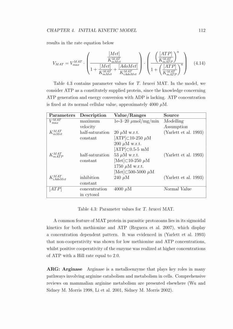
CHAPTER 5. PARAMETER ESTIMATION 166
As an example, Figure 5.11 shows that pairs such as (k6, k7) and (k9, k10) have
correlation values greater than 0.9, while pairs such as (k1, k7) and (k3, k9) have
correlations less than 0.01. To further illustrate the identification difficulties,
Figure 5.12 and Figure 5.13 present a fitness landscape of a two-parameterized
situation for a pair of the highest correlated parameters (k9, k10) and lowest cor-
related parameters (k6, k11), respectively. The first case shows a very long valley
along the diagonal of the parameters k9 and k10, reflecting the fact that there
exist many combinations of the values which can give an equally low value of the
objective function. The second case shows that, due to the lack of correlation,
there is a unique pair of values for k6 and k11 that corresponds to the minimum
of the objective function.
00.2
0.40.6
0.81.0 0
0.20.4
0.60.8
1.0
0.0
0.20.4
0.6
0.81.0
1.21.41.6
Parameter 9 Parameter 10
Obj
. Fun
ctio
n0.0
0.20.4
0.6
0.81.0
1.21.41.6
Figure 5.12: Objective function versus parameters k9 and k10, indicating thelarge parameter correlation.
In the context of optimization, a severe obstacle imposed by parameter corre-
lation is that some of the parameters are unidentifiable or identifiable but poorly
estimable. The latter refers to the situation where a small value of the objective
function can be obtained but some of the estimated parameters always have a
very large standard deviation. If this is the case, then the unidentifiable param-
eters would have to be fixed at measured values or at the best estimated values
in order to make the model structurally identifiable. Alternatively, models can

CHAPTER 5. PARAMETER ESTIMATION 167
00.2
0.40.6
0.81.0 0
0.20.4
0.60.8
1.0
0.0
0.51.0
1.5
2.02.5
3.03.54.0
4.5
Parameter 6 Parameter 11
Obj
. Fun
ctio
n
0.0
0.51.0
1.5
2.02.5
Figure 5.13: Objective function versus parameters k6 and k11, indicating a lackof identifiability.
be reduced further to remove unidentifiable parameters if necessary.
5.5.2 Practical Identifiability
Practical identifiability analysis arises due to limited amount and quality of
experimental data. Practical non-identifiabilities manifest as functionally related
parameters. The analysis examines the probability distribution of parameter
estimates by fitting a model repeatedly to data containing a certain degree of
noise and investigating the estimates.
The Hessian matrix, which contains the second derivatives of the objective
function with respect to the parameter estimates at convergence, is a common
means for testing the practical identifiability. The inverse of the Hessian matrix
gives the variance-covariance matrix of the parameter estimates, which enables
us to quantify the information content of an experimental data set (Faller et al.
2003). A basic procedure for constructing the FIM is presented in Appendix C.2.
The Hessian matrix is interesting in its own right. In gradient descent meth-
ods, the condition number of the Hessian gives an indication of the rate of
convergence and the impact of floating point rounding errors on the minimum

CHAPTER 5. PARAMETER ESTIMATION 168
objective function value (Thacker 1989). This number is defined as a ratio of its
largest to smallest eigenvalues. When the ratio is close to unity, the matrix is
well conditioned. However, in practice, the observable data is generally not rich
enough to allow for reliable estimation of all parameters. This causes an ill-posed
estimation problem, where a large uncertainty in the parameter estimates will
result.
We computed the gradient of the objective function, with each column of
the gradient corresponding to an individual system component, and calculated
the Hessian matrix. The eigenvalues of the Hessian matrix are used to deter-
mine whether a particular set of data is sufficient for parameter estimation. We
determined the information content of all the three sets of experimental measure-
ments (noise free) over 0–5, 5–10 and 0–10 minutes by calculating the condition
number of the Hessian matrix of the best fit estimated by each of the three data
sets. All the three data sets returned a condition number close to zero, with
the first data set (3.7973e-21) being slightly better than the others, and when
5% noise was added to the first data set, a condition number of 4.3305e-25 was
obtained. The tests indicate that the practical identifiability can be improved
by using transient and precise measurements.
The variance-covariance matrix is the key to parameter uncertainty analysis.
The conventional approach dependent on the Hessian matrix is not allowed when
there are non-identifiable parameters in the underlying model. Parameter non-
identifiability results in the Hessian matrix being singular, which causes the
probability distribution of the parameters to be asymmetric. It is fair to say
that the usefulness of Hessian matrix based approach is limited to studying
identifiable parameters only.
The subset of structurally identifiable parameters must be determined be-
forehand in order for the Hessian matrix approach to be useful. The technique
of Singular Value Decomposition can be employed towards this end. Refer to
Golub et al. (Golub et al. 1976) for technical details on the subject. Singular
value decomposition identified a subset of structurally identifiable parameters
(k1, . . . k6) for the model under investigation, which gives a condition number
1.7395e-07 using the first measurement set. This shows that, after removing the
rest of the parameters (k7, . . . k11), the original ill-posed problem is transformed
into a better conditioned problem.

CHAPTER 5. PARAMETER ESTIMATION 169
5.6 Conclusions and Discussion
In this chapter, we investigated the problem of parameter estimation for dynamic
biochemical systems. We gave an in-depth introduction to the theoretical back-
ground of optimization, and evaluated the usefulness of a global optimization
approach – Particle Swarm optimization and the derived method – the PSwarm
algorithm – in solving the inverse problem of non-linear systems. A careful anal-
ysis of an inverse problem related to the ERK signalling pathway was presented
as an illustrative example, where an error-free model structure was assumed.
The case study revealed the usefulness of PSwarm in tacking the problem of
ill-conditioning and multi-modality in parameter estimation.
By definition, parameter estimation involves using observed data to esti-
mate values of parameters based on statistical procedures. Parameter estimation
problems with measurement sets containing different information content were
analyzed. Noise in the measurements leads to noisy estimates of the parameters,
resulting in poor model predictions with the estimated solutions. This is most
prominent when using measurements providing the least information content.
We are aware of variations of standard PSO that are claimed to perform bet-
ter. A modern, well-tested variant (Gaussian Mutation) was implemented and
was also used in this study. In this case, we found that the Gaussian Mutation
variant takes more iterations to converge than with standard PSwarm. Accord-
ingly, standard PSwarm is chosen for the study of the trypanthione metabolic
pathway in Chapter 7. We emphasize that the prediction of correct system dy-
namics is more important than the accuracy of the estimated parameters when
evaluating the performance of the algorithms.
We conducted an analysis of model identifiability and examined the impact
of prior structural knowledge and the quality of experimental measurements on
the parameterization issue. Model identifiability analysis explains the challenges
of estimating parameters for non-linear systems where the parameters are poten-
tially highly correlated. It concluded that the ERK signalling pathway is neither
structurally or practically identifiable, since there are pairs of parameters that
are significantly correlated. Such analysis can guide the estimation problem by
suggesting biological experiments for measuring parameters that are dependent
on each other, or by removing parameters via model reformation for a better
identifiability property.
The challenge of parameter estimation using experimental measurements
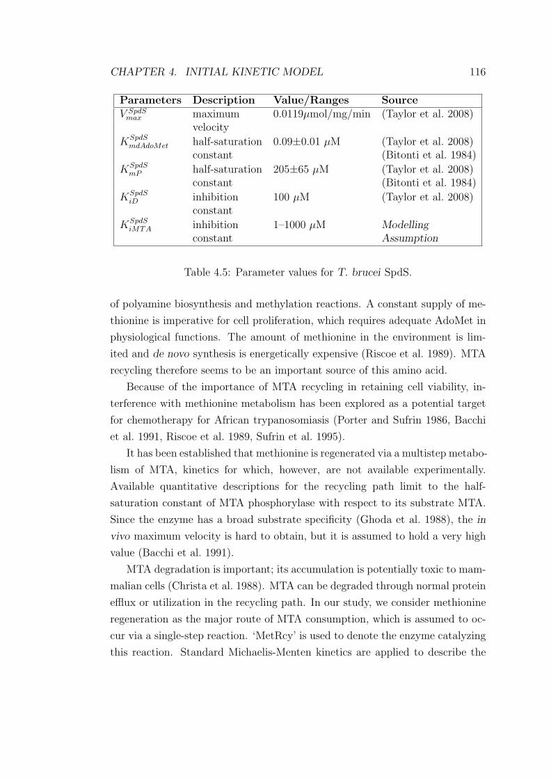
CHAPTER 5. PARAMETER ESTIMATION 170
that suffer from a poor information content (i.e. steady-state data) is addressed
in Chapter 6. We propose an approach that tackles this problem by coupling
transient data, which is rich in information, with steady-state data in the calibra-
tion procedure. The proposed approach can be generalized to solve a variety of
multi-objective optimization problems constrained by more than one condition,
which is particularly useful for model validation of biological systems where the
observed data for parameter estimation is measured in the perturbed condition
of the system. The proposed approach is applied to solve the inverse prob-
lem of the polyamine biosynthetic sub-pathway of the trypanothione metabolic
pathway in Chapter 7.
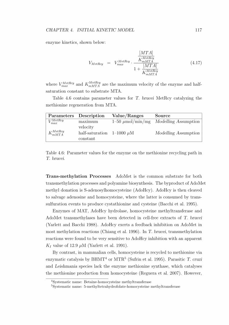
Chapter 6
MoPSwarm: The Proposed
Approach for Perturbation-based
Model Validation
In this chapter we propose a novel approach for applying a multi-objective op-
timization to validation of perturbation-based models of biological systems. We
compare the results from the proposed approach with those from the conven-
tional validation procedure.
6.1 The Challenge
It is necessary to be able to accurately and reliably determine values for system
parameters in order to develop predictive models (van Riel 2006). This is espe-
cially important when the dynamic behaviour of a system is highly dependent
on parameter values. Parameter estimation is therefore an important research
area in Systems Biology.
Parameter estimation is a particularly complex task when the validation of
a biological system can only be achieved by comparing simulation results with
measurements from perturbation experiments. A common approach to model
validation involves a two-step procedure to determine the vector of estimated
parameters that can correctly describe a system’s responses to perturbations.
This involves fitting model parameters to experimental data generated by a
reference cell type (wild type) and then testing this model on data generated by
a variation (mutant). Parameter estimation is one building block of the model
171

CHAPTER 6. MULTI-OBJECTIVE PSWARM 172
validation procedure.
For the trypanothione metabolic pathway under investigation, the drug in-
hibitor DFMO, which degrades the activity of enzyme ODC, was added to the
cell after the cell reached steady state. When solving the model of trypanothione
metabolism, a decision vector p that can be considered as a potential solution
for the unknown parameters should satisfy two constraints:
1. Simulation results of the model with p should be consistent with the ob-
served steady state (wild type)
2. When the parameter of interest in p is perturbed with a certain percentage
that constitutes the perturbed vector p, simulation results of the model
with p should be consistent with the measured perturbation data (mutant).
It is well-known that a major difficulty in estimating model parameters from
the steady-state data (as the reference cell type) lies in the fact that a potentially
very large number of different values can be obtained for the model parameters,
showing equally good consistency with the experimental data. This frequently
makes the common approach infeasible in practice. From the perspective of
parameter estimation, this difficulty arises from the lack of information contained
in the wild-type data used for this purpose, as discussed in Chapter 5. An
intuitive way to solve the problem is to use informative data, for example, the
transient concentrations of the system components, to optimize the parameters
with respect to a mutant and then test potential solutions against the wild-type
cell. Again, the challenge is still present regarding whether or not the decision
vector can meet the steady-state constraint.
Existing implementations of multi-objective optimization with Particle Swarm
(MOPSO) have never been applied to complex real-world applications, by which
we mean the applications involving a large number of decision variables and
dependent on differential equations to describe the system dynamics. Even
the most up-to-date MOPSO implementation by Rabbani et al. (Rabbani
et al. 2009) was initially designed for solving the project selection problem,
formulated as a set of time-independent algebraic equations parameterized with
binary (0 and 1) decision variables.
In this chapter, we thus propose a novel approach for the application of multi-
objective optimization using Particle Swarm for the validation of perturbation-
based models of biological systems. This implementation is inspired by the

CHAPTER 6. MULTI-OBJECTIVE PSWARM 173
single-objective optimizer, PSwarm, which is designed in a Search-and-Poll frame-
work. With the proposed approach, the constraints arising from both the steady-
state condition (wild type) and the perturbed condition (mutant) are handled
simultaneously. In the following sections, the theoretical background of multi-
objective optimization is introduced and our proposed approach is described and
evaluated using the ERK signalling pathway as a case study. The pathway was
studied in detail in Section 5.4 in Chapter 5.
6.2 Multi-objective Optimization
This section provides the necessary background for the work on multi-objective
optimization, which is described later. Some of the basic concepts in multiob-
jective optimization are introduced and the visualization of approximate non-
dominated solutions, as produced by the proposed multi-objective optimizer, is
also presented. The theoretical background related to multi-objective optimiza-
tion is explained based on descriptions given by Fonseca and Fleming (Fonseca
and Fleming 1995) and Coello (Coello 2001).
Most problems in nature have several, possibly conflicting, objectives to be
satisfied. Many of these problems are frequently treated as single-objective op-
timization problems by transforming all but one objective into constraints.
Multi-objective optimization attempts to find a solution to more than one
objective function simultaneously. Specifically, the Multi-objective Optimization
problem can be defined as the problem of finding a solution which would give
values for all objective functions that are acceptable to the performance criteria
(Osyczka 1985). Specifically, multi-objective optimization attempts to find a
vector of decision variables X that optimizes a vector function F
F (X) = [f1(X), f2(X), . . . , fk(X)]T (6.1)
whose elements represent each individual objective function, fi(X).
Multi-objective optimization intends to seek good compromises (or trade-
offs), which are Pareto optimum, rather than a single solution as in conventional
global optimization. By definition, X∗ is Pareto optimal if there exists no feasible
vector of decision variables X ∈ R which would improve one performance criteria
without causing a simultaneous degradation of performance in at least one other
criterion. More precisely, we have the following definition.
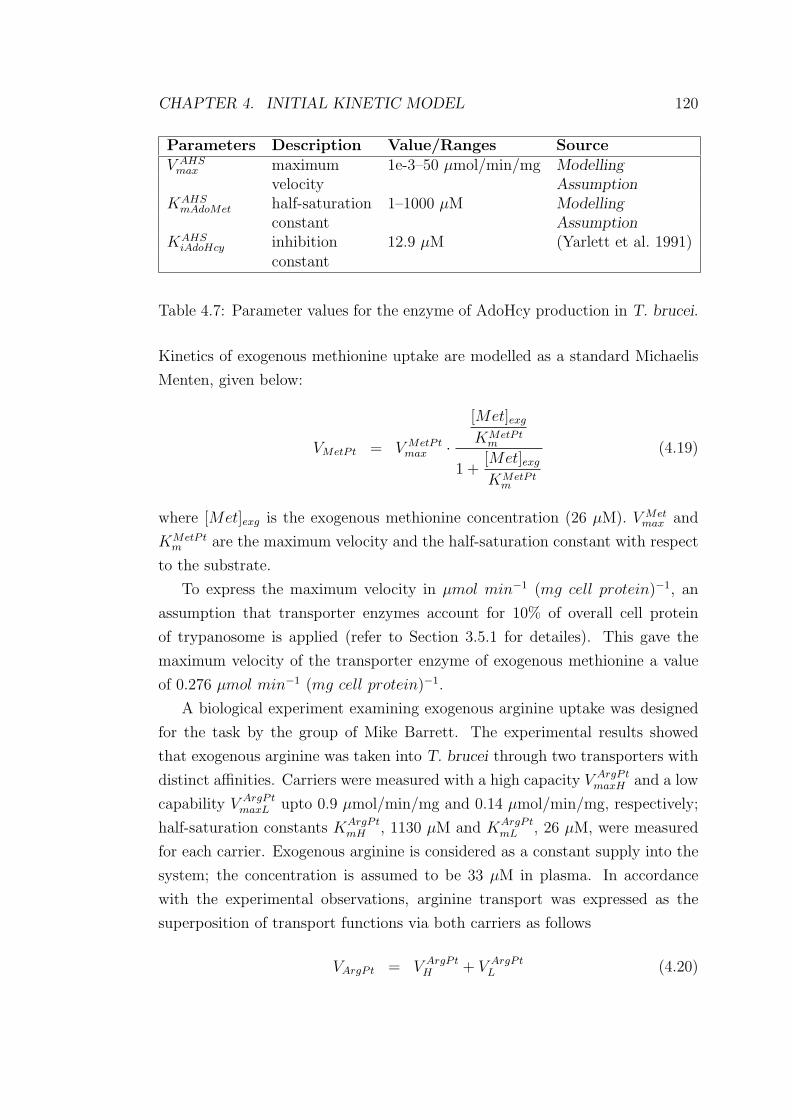
CHAPTER 6. MULTI-OBJECTIVE PSWARM 174
Definition 6.1 (Pareto Optimum): We say that a vector of decision variables
X∗ ∈ R is Pareto optimal if there does not exist another X ∈ R such that fi(X) ≤fi(X
∗) for all i ∈ 1, . . . , k and fj(X) < fj(X∗) for at least one j ∈ 1, . . . , k. Here
R denotes the feasible region of the the problem, where all constraints are satisfied.
The concept defines a set of solutions that is the so-called Pareto optimum
set. The vectors X∗ corresponding to the solutions included in the Pareto opti-
mal set are referred to as non-dominated solutions1. The objective functions of
non-dominated solutions in the Pareto optimal set form the Pareto front, which
can be purely/partially convex, concave or discontinuous. Approximation of the
Pareto front is sometimes referred to as Pareto optimization. If we plot the
objective functions (for two objectives) of the Pareto-optimal solutions, then we
can obtain a Pareto front as shown schematically in Figure 6.1.
0 20 40 60 80 100Objective 1
0
100
200
300
400
Obj
ectiv
e 2
P2
P3
P1
Figure 6.1: An ideal Pareto front for two objective functions is formed with filledcircles in this figure. The rough curve in filled triangles can be understood as anintermediate front resolved during the course of search process. Test particleslabelled with P1, P2 and P3 illustrate different types of solutions. Refer to thetext for a full explanation.
Figure 6.1 indicates that a solution lying on the Pareto-optimal frontier can-
1We will clarify later how to interpret ‘non-dominated solutions’ in this context.

CHAPTER 6. MULTI-OBJECTIVE PSWARM 175
not improve one objective without sacrificing performance in the other. In a
cost-effective scenario, no better performance can be possibly achieved without
increasing cost. Given the constraints of the problem, no solutions can exist in
the region below the front. All possible solutions located in the region above
the front are defined as non-Pareto optimum indicated with filled triangles in
Figure 6.1. As the search continues, the intermediate trade-off curve moves to-
wards the true Pareto front in the possession of a smoother appearance. It is
worth emphasizing that when solving real-world applications, no Pareto front
can be as smooth as it is presented in Figure 6.1 (filled circles); a real example
is demonstrated by Figure 6.3.
A different group of methods for solving multi-objective optimization prob-
lems do not incorporate directly the concept of Pareto optimum. A represen-
tative of non-Pareto approaches is the Aggregation Function, which combines
all objectives into a single objective by using addition, multiplication or any
other combination of arithmetical operators. Individual objective functions are
frequently assigned a weighting value to distinguish the significance of different
objectives. Non-Pareto approaches are simple and easy to implement but they
are unable to produce certain segments of the Pareto front and are limited to
handling only a few objectives. Linear combinations of weights are not appli-
cable when the Pareto front is concave, regardless of the weights used (Fonseca
and Fleming 1995).
Related work on aggregation functions by van Riel and Sontag (van Riel
and Sontag 2006) studied the metabolic regulation in Saccharomyces cerevisiae
when different nitrogen pulses are added to the cell at a number of time points.
Model parameters were estimated via a constrained optimization method, where
solutions are subject to constraint(s). The model was optimized by minimizing
the difference between the experimental data and model output in a least-squares
criterion subject to the constraint of steady-state condition implemented as the
sum of squares. These two identification criteria are added together as the overall
fitness function to be adjusted by the optimizer. van Riel and Sontag again
raised the issue that it is difficult to define the relative importance of different
objectives in a multi-objective criterion and the decision is always somewhat
subjective.

CHAPTER 6. MULTI-OBJECTIVE PSWARM 176
6.2.1 Multi-objective Particle Swarm Optimization
Particle Swarm Optimization (PSO) is one of the newest techniques in the
family of evolutionary algorithms, motivated by the simulation of social be-
haviour. PSO is particularly suitable for multi-objective optimization due to
the high convergence rate of the algorithm. This is discussed in the context
of single-objective optimization in Chapter 5. Due to the population-based na-
ture of PSO, it appears to be fairly straightforward to transform the algorithm
to solve multi-objective optimization problems using a ‘Pareto ranking scheme’
(Goldberg 1989). However, only a few works have been recently proposed for
MOPSO.
The application of evolutionary algorithms into multi-objective optimization
has been under investigation since the mid 1980s, and is largely centered on Ge-
netic Algorithms (Fonseca and Fleming 1993, da Fonseca 1995, Deb et al. 2000).
For example, da Fonseca (da Fonseca 1995) has applied the multi-objective ge-
netic algorithm to a subset selection problem. The selection criteria constrained
by the objectives of residual variance and mean-square prediction error are used
in the selection of appropriate non-linear terms for polynomial models of a pilot
scale liquid-level system. In their study, a large number of 1000 input-output
pairs are employed for the optimization process.
Evolutionary algorithms deal with a set of possible solutions simultaneously.
This is particularly suitable for coping with multi-objective optimization prob-
lems, where the search of the Pareto optimal set may be achieved in a single
run of the algorithm. Evolutionary algorithms are also less susceptible to the
shape or continuity of the Pareto front (Coello 2001). This corresponds to the
problem of concavity and discontinuity when solving optimal vectors over a high-
dimentional search space.
Fieldsend (Fieldsend 2004) compared the proposed techniques for MOPSO
(Hu and Eberhart 2002b, Parsopoulos and Vrahatis 2002a, Coello and Lechuga
2002, Fieldsend and Singh 2002, Mostaghim and Teich 2003). These methods
mainly differ in the two aspects, namely: the use of an external ‘repository’ for
non-dominated solutions, which is retrieved by every particle after each flight
cycle; and the selection of personal best (pbest) and global best (gbest) particles
for each particle in the population. In Fieldsend’s review, the impact of selec-
tion strategies for particles on the convergence rate and diversity of solutions is
emphasized when solving a number of objectives simultaneously.
A recent and comprehensive survey on the state-of-the-art of multi-objective

CHAPTER 6. MULTI-OBJECTIVE PSWARM 177
optimization with PSO is also provided by Reyes-Sierra and Coello (Reyes-Sierra
and Coello 2006). The key issues related to the extension of PSO to multi-
objective optimization scheme are detailed in the survey, and include:
1. How to ensure the diversity in the solutions found in order to obtain a
smooth and uniform distribution and to avoid convergence to a single
solution;
2. How to determine, retain and update the non-dominated solutions during
the search process;
3. How to select leader particles to guide the global search;
Reyes-Sierra and Coello underlined the fact that even though MOPSOs have
been used in a few applications, they are almost never employed as a pri-
mary search engine in solving the real-world applications. This survey urges
researchers from this domain to develop well-designed multi-objective optimizers
in order to effectively solve real-world applications. The usefulness of MOPSOs
should be examined with respect to the capability of the algorithm in producing
reasonably good approximations of the Pareto front when applied to real-wold
multi-objective optimization problems. For instance, applications that include
a large number of decision parameters and time-dependent behaviour of system
components is of interest. This is in contrast to the relatively simple algebraic
equations for which MOPSOs were initially designed and tested with. The lack
of relevant applications may explain why, despite a fast growth of this field,
MOPSO techniques have not yet been widely used in practice.
In the following sections, we provide a detailed description of the proposed
approach for solving complex multi-objective optimization problems. The per-
formance of the approach is evaluated using the ERK signalling pathway as a
case study.
6.2.2 Basic Concepts
In this section we define several mathematical terms used in this chapter in order
to establish a common terminology.
Definition 6.2 (Weak Dominance): A decision vector x∗ from a feasible region
S ∈ R is said to weakly dominate a decision vector x ∈ S (denoted x∗ � x) iff: the

CHAPTER 6. MULTI-OBJECTIVE PSWARM 178
decision vector x∗ is not worse than x in all objectives, stated as fi(x∗) ≤ fi(x) for
i = 1, . . . , k.
Definition 6.3 (Strong Dominance): A decision vector x∗ from a feasible region
S ∈ R is said to strongly dominate a decision vector x ∈ S (denoted x∗ ≺ x) iff:
(i) the decision vector x∗ is not worse than x in objectives where fi(x∗) ≤ fi(x) for
i = 1, . . . , k and (ii) the decision vector x∗ is strictly better than x in at least one
objective where fi(x∗) < fi(x) for i = 1, . . . , k.
Definition 6.4 (Fully Dominated Solutions): A decision vector y is termd a fully
dominated solution with respect to a test vector x iff; the decision vector y is worse
than x in all objectives, i.e. fi(y) > fi(x) for i = 1, . . . , k.
Definition 6.5 (Partially Dominated Solutions): A decision vector y is termed
a partially dominated solution with respect to a test vector x iff; (i) the decision
vector y is strictly better than x in at least one objective, i.e. fi(y) < fi(x) for
i = 1, . . . , k and (ii) the decision vector y is no worse than twice of the objective
value of x in all other objectives, i.e. fi(y) ≤ 2 × fi(x) for i = 1, . . . , k.2
Definition 6.6 (Non-dominated Solutions): A decision vector y is termed a non-
dominated solution with respect to a test vector x iff; the decision vector y is strictly
better than x in all objectives, i.e. fi(y) < fi(x) for i = 1, . . . , k.
It should be emphasized that different types of solutions (e.g. fully domi-
nated, partially dominated and non-dominated solutions) must be defined with
respect to a test particle. As illustrated by Figure 6.1, particle P1 and P3 are
non-dominated solutions with respect to particle P2, and conversely, P2 is a fully
dominated solution with respect to P1 and P3. Particle P1 and P3 are mutually
partially-dominated solutions, as neither solution is superior to the other. Solu-
tions lying on the true Pareto-optimal front should fully dominate all the other
points ‘inside’ the front but partially dominate each other. In other words, no
other solutions in the search space are superior to the Pareto-optimal solutions.
2The choice of ‘2× fi(x)’ is arbitrary and can be changed. This is to avoid the selection ofparticularly bad particles.
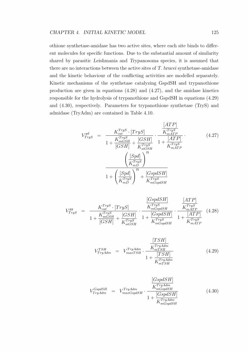
CHAPTER 6. MULTI-OBJECTIVE PSWARM 179
6.3 Description of the Proposed Approach for
Multi-objective Optimization
The currently proposed approach for multiple-objective optimization is based
on the Search-and-Poll framework adopted in the single-objective optimizer
PSwarm, which is a generalized pattern search algorithm – in the search step
standard PSO is employed and the poll step is only activated when the search
step failed.
Our proposal is based on the strategy of having an external repository (also
termed as the archive in this chapter) in which every particle can deposit its flight
experiences after each flight cycle3. The mechanism of crowding distance com-
putation is incorporated in the multi-objective optimization with PSO (Raquel
and Naval 2005) for the purpose of selecting the global best particle.
The crowding distance computation provides an estimate of the density of
solutions surrounding a particular solution in the population (Deb et al. 2000).
It estimates the size of the largest rectangle (or higher dimensional equivalent)
enclosing the solution i without including any other solution in the population.
The crowding distance of a particular solution takes the average distance of its
two neighboring solutions, which helps distribute particles uniformly over the
search space. This computation is carried out for each objective, and the final
distance measure of a solution is computed by adding the individual crowding
distance values calculated for each objective. The pseudo code of the mechanism
(for an individual objective) is given in Algorithm 2, based on the description
by Deb et al. (Deb et al. 2000).
One distinct feature of the proposed approach which we shall call ‘MoP-
Swarm’ is the employment of a Poll step in seeking non-dominated solutions.
The Poll step is used in order to provide more opportunities to gain satisfac-
tory convergence and ensure a good diversity. The problems we are interested
in solving with MoPSwarm are Bound Constrained Optimization problems, the
definition of which was given in Section 5.2.1 in Chapter 5.
In multi-objective optimization, a set of non-dominated solutions represent-
ing the best individuals found so far during the search process replaces the single
global best particle in the single-objective optimization case. This leads to a de-
3In practice, two external repositories are required, one stores the non-dominated solutionsand the other stores the decision variables corresponding to non-dominated solutions. Therepository of non-dominated solutions is manipulated through the searching process, and theother repository should be updated accordingly.

CHAPTER 6. MULTI-OBJECTIVE PSWARM 180
Algorithm 2 Crowding Distance Computation (Deb et al. 2000).
1: Get the number m of non-dominated solutions in the archive REP2: Initialize distance value of each non-dominated solution DistanceREP (i) to
zero for all m stored solutions3: for i = 0 to m do4: Sort the solutions in descending order of the objective value5: Set infinite crowding distance values to the lowest and highest objective
function values DistanceREP (1) = DistanceREP (m) = ∞6: for j = 2 to m − 1 do7: Calculate the average distance of each particle solution us-
ing the formula DistanceREP (j)=DistanceREP (j)+(DistanceREP (j+1) −DistanceREP (j−1))
8: end for9: end for
cision whether an external repository is used to store non-dominated solutions
that are retrieved by every particle after each flight cycle.
MoPSwarm incorporates an external repository (REP ) with a filtering pro-
cess that encourages a uniform distribution of solutions along the Pareto front.
No limit is imposed on the maximum number of solutions that REP can store.
REP is initialized with the objective function values of the initial particles and
the global best guide particle is then selected from a set of Pareto-optimal solu-
tions via distinct selection strategies.
The proposed algorithm is summarized in Algorithm 3.
6.3.1 Local Best Selection
Choosing pbest and gbest particles to direct a swarm member’s flight is not triv-
ial in multi-objective optimization with PSO (Fieldsend 2004). In MoPSwarm,
the selection criteria for pbest for individual particles follows the rule of Strong
Dominance. At each iteration of the flying cycle, for each individual particle,
the position that fully dominates the previous position is recorded. The Poll
step is activated if the search for a local best guide fails at the Search step. In
the Poll step, members in a finite set of trial points are examined in turn and
selected in accordance with the rule of Strong Dominance. The pseudo code for
the selection of local best guide is summarized in Algorithm 4.

CHAPTER 6. MULTI-OBJECTIVE PSWARM 181
Algorithm 3 MoPSwarm: A general algorithm for multiple-objective optimiza-tion1: Choose a population size s and termination criteria. Randomly initialize
the initial particles in the population x1(0), . . . ,xs(0) with initial local bestpositions y1
lb(0), . . . ,yslb(0) and the initial velocities v1(0), . . . ,vs(0).
2: Initialize the external repository REP with f 1(z), . . . , fk(z), wherez ∈ x1(0), . . . ,xs(0) for k objectives
3: while Termination criteria are not met do4: Search for personal best positions, pbest, for individual particles in the
population (defined in Section 6.3.1) using the Search-and-Poll framework5: Update the external repository REP (defined in Section 6.3.3) using the
Search-and-Poll framework6: Refresh the external repository REP every nr iterations (defined in Sec-
tion 6.3.4)7: Select a global best particle, gbest, from REP to guide flying of each
particle in the population (defined in Section 6.3.2).8: Update velocities of individual particles in the population with the formula
x(t + 1) = x(t) + v(t).9: end while
6.3.2 Global Best Selection
As illustrated by Fieldsend (Fieldsend 2004), the selection strategies for gbest to
guide the search of the next cycle fall into two categories, namely ‘unrestricted’
and ‘restricted’ groups. The former allows the selection of members freely from
the external repository, whilst the latter restricts the selection of gbest using
some form of distance measure.
Each method has it own advantages and disadvantages, and often one method
compensates for another’s deficiency. The unrestricted selection of gbest helps
avoid ‘clumping of particles’ and prevents particles from becoming trapped
within limited areas of the search space. However, this method will proba-
bly accept particles with ‘bad’ positions as the leading particle, thus requiring
more computational time on average to converge. The restricted gbest selection
may promote clumping of particles, but a good set of non-dominated solutions
is more likely to be obtained at each iteration.
In our proposed approach, both strategies of ‘unrestricted’ and a geographically-
based selection (Crowding Distance) strategy are examined. With the restricted
selection strategy, a non-dominated solution from the top 10% least crowded
area of the archive is randomly chosen as the global best guide. A different
gbest is selected for each particle in the population.
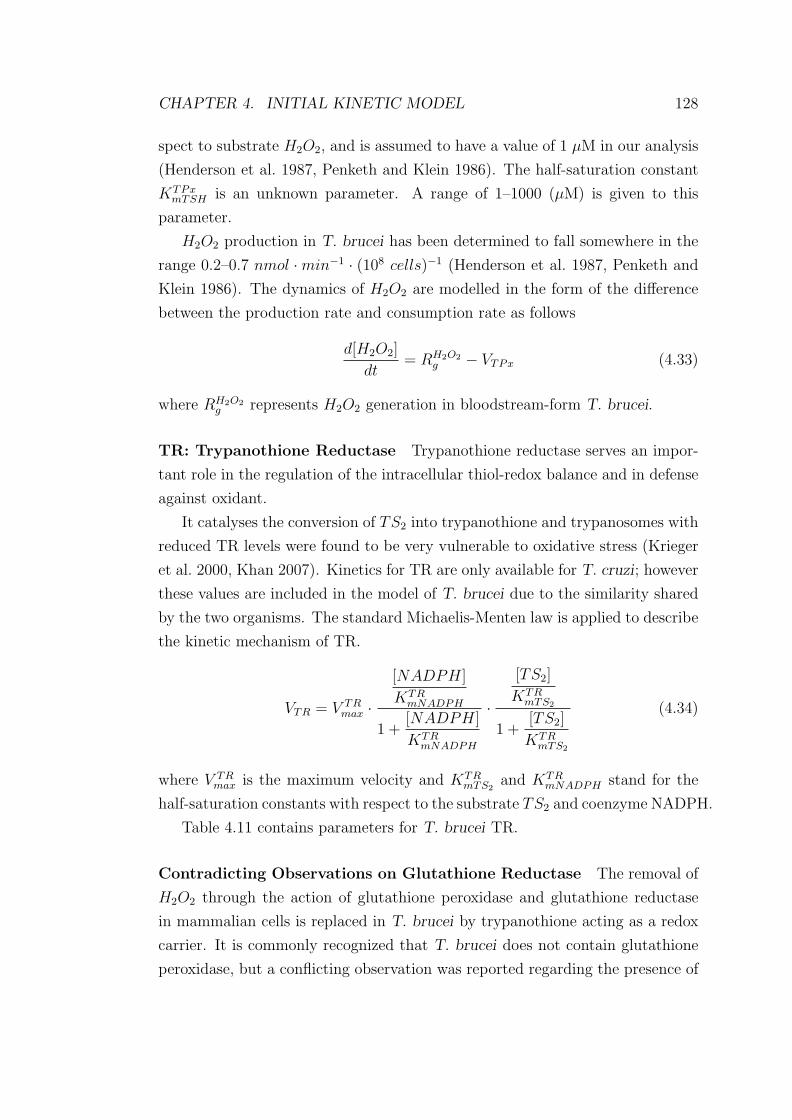
CHAPTER 6. MULTI-OBJECTIVE PSWARM 182
Algorithm 4 Search for local best guide
1: [Search Step]2: for i = 1, . . . , s do (for every particle i): do3: Compute f(xi(t)) for each objective j ∈ 1, . . . , k4: if the decision vector xi fully dominates yi
lb then5: Set yi
lb(t + 1) = xi(t) (update the particle i local best position; searchstep successful)
6: Reset the search direction for pattern search7: end if8: [Poll Step]: Skip the poll step if the search step was successful.9: Choose the spanning set D.
10: if there exists d(t) ∈ D such that f(yilb(t) + αi(t)d(t)) is a non-dominated
solution with respect to f(yilb(t)) then
11: Set yilb(t + 1) = yi
lb(t) + αi(t)d(t) (a new local best position found forthe particle; poll step successful)
12: Set αi(t + 1) = φ(t)αi(t) (increase the mesh size parameter accordingto the rule in Equation (5.3))
13: else14: Set yi
lb(t+1) = yilb (No change in the local best position for all d(t) ∈ D;
poll step unsuccessful)15: Set αi(t + 1) = θ(t)αi(t) (decrease the mesh size parameter according
to the rule in Equation (5.4))16: end if17: end for
6.3.3 Updating the Archive
In the scheme of multi-objective optimization, the definition of ‘superior’ par-
ticles for the update of the archive REP is a critical consideration, which may
have a major influence on the convergence of the algorithm and the diversity of
the Pareto-optimal solutions. In our proposed approach, two different updating
strategies are applied and the resulting optimization performance is assessed.
The two proposals are termed Strong-Dominance and Weak-Dominance up-
dating strategies, which specify that during the search process
1. With the strong-dominance updating strategy, only the particles that are
non-dominated by the stored solutions in the archive are inserted and the
corresponding dominated solutions in the archive are deleted.
2. With the weak-dominance updating strategy, particles that are non-domin-
ated or partially dominated by the stored solutions in the archive are
inserted and only fully dominated stored solutions are deleted.

CHAPTER 6. MULTI-OBJECTIVE PSWARM 183
The Pseudo code of the Weak-Dominance updating strategy is summarized
in Algorithm 5. The description in Algorithm 5 can also be used to refer to the
Strong-Dominance updating strategy, where for the latter partially dominated
solutions are not accepted in the Poll step (see statement 19 in the algorithm).
Algorithm 5 Weak-dominance updating strategy of the archive REP
1: [Search Step]2: for i = 1, . . . , s do (for every particle i): do3: Compute f(xi(t)) for each objective j ∈ 1, . . . , k4: if the current particle f(xi(t)) fully dominates the stored solution(s) in
REP then5: Remove the dominated stored solutions from REP and insert f(xi(t))
into REP6: Retain the remaining stored solutions in REP ; search step successful7: end if8: if the current particle f(xi(t)) partially dominates the stored solution(s)
in REP then9: The current particle is retained for the Poll step
10: No update is made to the archive REP ; search step unsuccessful11: end if12: if the current particle f(xi(t)) is fully dominated by the stored solution(s)
in REP then13: No update is made to the archive REP ; search step unsuccessful14: end if15: end for16: [Poll Step]: Skip the poll step if the search step was successful.17: Choose the spanning set D.18: For dn(t)n=[1,...,m] ∈ D find f(yi(t) + α(t)d(t)) ∈ arg minn∈[1,...,m]f(yi(t) +
α(t)dn(t))19: if there exist f(yi(t)+α(t)d(t)) that fully dominates or partially dominates
f(yi(t)) then20: Set yi(t) = yi(t) + αi(t)d(t) and f(yi(t))=f(yi(t) + α(t)d(t))21: Remove the dominated solution(s) stored in the archive REP22: Insert the solution f(yi(t)) into the archive REP (update of the archive
REP is done; poll step successful)23: Set αi(t + 1) = φ(t)αi(t) (increase the mesh size parameter according to
the rule Equation (5.3)).24: else25: No update is made to the archive REP ; poll step unsuccessful26: Set αi(t + 1) = θ(t)αi(t) (decrease the mesh size parameter according to
the rule in Equation (5.4)).27: end if

CHAPTER 6. MULTI-OBJECTIVE PSWARM 184
6.3.4 Refreshing the Archive
In MoPSwarm, a check on the archive REP is performed every nr=10 iterations4
during the search process. The Pareto-optimal subset of the current archive is
saved and all other (fully dominated) solutions are eliminated. The possibil-
ity that fully dominated solutions are inserted into the archive arises from the
mechanism that we applied to the update of the archive, which is that the Poll
step may accept potentially inferior solutions for the sake of diversity. This re-
fresh step can help form a better Pareto-optimal front by eliminating the fully
dominated solutions from the archive.
6.3.5 Termination Criteria
The maximum number of iterations is a commonly used stopping criterion for
evolutionary algorithms. To ensure a proper termination in practice, in the
proposed approach, we introduce a mechanism for deactivating particles when
the mean magnitude of changing position of the particle within two neighboring
iterations is smaller than the tolerance (1e-5).
Our experiences from experimental testing of MoPSwarm suggest that it is
possible that under some conditions the expected value of the norm of the veloc-
ities vectors tends to zero for most of the particles after being through enough
iterations of the search process. These particles will have less contribution to
the global parameter search for their low search activity. Deactivated particles
from the previous iteration will be removed from the population and won’t be
considered in the subsequent search process.
In the implementation, no particle deactivation is permitted in the first five
iterations of the search cycle, which is designed to allow the particles with small
initial velocity values to start moving. The algorithm terminates when there
is only one particle remained in the population. The mechanism of particle
deactivation can not only save the computational resources by removing the
particles that don’t show enough movement, but also promote a satisfactory
convergence of other particles to the true Pareto front by preventing them from
being trapped by the inactive particles.
4Note that 10 interations is arbitrary and can be changed.

CHAPTER 6. MULTI-OBJECTIVE PSWARM 185
6.4 Case Study: ERK Signalling Pathway
To demonstrate the usefulness of MoPSwarm in solving the inverse problem
of the ERK signalling pathway, a comparison of model validation via both the
common approach and the proposed approach is carried out. The computational
model of the pathway was given in Table 5.1 in Chapter 5.
Regardless of which approach is used, true perturbation data for the ERK
signalling pathway has to be available beforehand. This can be the data de-
scribing the perturbation experiment applied to an arbitrary model parameter.
To obtain a perturbation of the model, we applied a 90% knockdown of each
parameter from its reference value, one at a time, and simulated the model with
the mutated parameter set for perturbation data. The initial conditions and
the reference parameter values for the model simulations are fixed at the num-
bers reported in Chapter 5. Each perturbation data set contains the transient
concentrations of the system’s components at 11 time points evenly spacing the
time span between 0 and 100 minutes.
We observed that under these perturbed conditions some of the parameters
have negligible effects on the change of concentrations of the system’s compo-
nents. To better demonstrate the prospects for experimental design considera-
tions, only the perturbation data exhibiting an evident impact on the system’s
dynamics is retained. The perturbation data to be used as the ‘true’ data in the
second step of model validation was generated with the parameter set where k8
was mutated to 10% of the reference value, and the remaining parameters were
unchanged.
The ODEs of the pathway used in the perturbed condition are shown in
Table 6.1, where k∗8 is expressed as k8 · β. Here, β represents the perturbation
applied to the parameter of interest (k8).
In this in silico study, the initial condition of the pathway is considered as an
unknown parameter so as to mimic a realistic situation, where prior knowledge
about the system is at best partial. This consideration leads to 22 unknown
parameters to be estimated in total. All unknown kinetic parameters were as-
sumed to vary between 0 and 1. Values of the initial concentrations of the
system’s components are restricted to ±20% of the given steady state to help
the convergence of the algorithm from random positions in the search space.
Following the conventional approach, a set of parameters that can satisfy
the steady-state constraint of the pathway was solved using the global optimizer
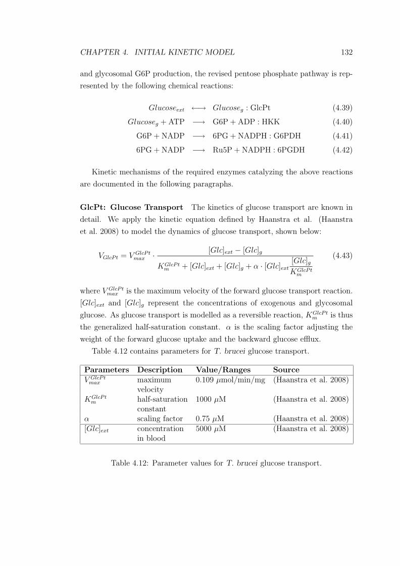
CHAPTER 6. MULTI-OBJECTIVE PSWARM 186
Reaction number Kinetic equations
1 −k1 · m1 · m2 + k2 · m3 + k5 · m4
2 −k1 · m1 · m2 + k2 · m3 + k11 · m11
3 k1 · m1 · m2 − k2 · m3 − k3 · m3 · m9 + k4 · m4
4 k3 · m3 · m9 − k4 · m4 − k5 · m4
5 k5 · m4 − k6 · m5 · m7 + k7 · m8
6 k5 · m4 − k9 · m6 · m10 + k10 · m11
7 −k6 · m5 · m7 + k7 · m8 + k∗8 · m8
8 k6 · m5 · m7 − k7 · m8 − k∗8 · m8
9 −k3 · m3 · m9 + k4 · m4 + k∗8 · m8
10 −k9 · m6 · m10 + k10 · m11 + k11 · m11
11 k9 · m6 · m10 − k10 · m11 − k11 · m11
Table 6.1: The ODE-based computational model of ERK signalling pathway.
PSwarm for the simulation study. Two hundred runs of the steady-state op-
timization were executed in Matlab. Each run starts with a different initial
population of particles and is computed over a simulated time span of 200 min-
utes. The set of parameters, P∗, which gives the smallest value of the objective
function, is retained. P∗ is given below:
k1 = 1, k2 = 0.1880, k3 = 0.8015, k4 = 0.0437, k5 = 1e − 6, k6 = 0.9970,
k7 = 0.1014, k8 = 1e − 6, k9 = 0.9758, k10 = 0.9903, k11 = 1e − 6.
m1|t=0 = 0.3090, m2|t=0 = 0.2320, m3|t=0 = 0.6274, m4|t=0 = 1.5646,
m5|t=0 = 0.03099, m6|t=0 = 0.01487, m7|t=0 = 1.7822, m8|t=0 = 0.7169,
m9|t=0 = 0.1907, m10|t=0 = 2.9364, m11|t=0 = 0.0610.
To test if P∗ is able to reproduce the true perturbation data, a 90% knock-
down is applied to the estimated value of k8 in P∗, which forms the mutated
parameter set, p∗. The model dynamics under the perturbed condition are ap-
proximated with p∗, where the initial condition for model simulation correspond
to the final values of the steady-state model computed with P∗.
The predicted perturbation profiles of Raf1/RKIP, Raf1/RKIP/ERK, MEK-
PP and MEK-PP/ERK are shown in Figure 6.2. The other system components
do not present dynamic changes in response to k8 knockdown and are therefore
omitted from the figure. This figure indicates that with the common approach,
even the ‘best’ set of parameters estimated from the steady state failed to pro-
duce satisfactory results compared with the true perturbation data.

CHAPTER 6. MULTI-OBJECTIVE PSWARM 187
0 20 40 60 80 100Time (mins)
0.5
1
1.5
2
Con
cent
ratio
n (A
rb. U
nits
)Raf1/RKIPRaf1/RKIP/ERKMEK-PPMEK-PP/ERKSimulationReal Data
Figure 6.2: Comparison of the simulated perturbation profile (continuous lines)with the true perturbation data (dotted lines). Note that concentration profilesonly match at t = 0.
6.5 A Comparative Study of MoPSwarm
In this section, we investigate the performance of several variants of MoPSwarm
in solving the multi-objective optimization problem of ERK signalling pathway.
The variants differ in the strategy used for selection of the global best guide
and in whether the archive REP is refreshed. The weak-dominance updating
strategy was adopted in all the MoPSwarm variants, which are summarized
below
• Variant 1: The crowding distance computation is adopted and the archive
is not refreshed.
• Variant 2: The unrestricted selection technique is adopted and the archive
is refreshed every 10 iterations.
• Variant 3: The unrestricted selection technique is adopted and the archive
is not refreshed.
• Variant 4: The crowding distance computation is adopted and the archive
is refreshed every 10 iterations.

CHAPTER 6. MULTI-OBJECTIVE PSWARM 188
Solutions computed with the four variants of MoPSwarm are presented in
Figure 6.3, and the corresponding Pareto front is convex. Note that the scales
are different in each of these plots, indicating significant differences in the range
of the objective function values. The maximum number of iterations was set to
100 and 20 particles were used in the initial population. Both objectives of the
steady-state and perturbed condition are formulated using the penalized likeli-
hood error criterion, in which the error increases exponentially as the distance
between the estimated and observed value increases. The penalized likelihood
error criterion is expressed as follows for time points i = 1, . . . , m and system
components j = 1, . . . , n:
minimize ε =∑
1≤i≤m
∑1≤j≤n
1
fij
(6.2)
where fij is defined as a Normally distributed probability density function, with
a mean of the experimental measurement yD(ti, xj) and a standard deviation σ
of 1. This is given as follows
fij =1√
2πσ2exp
(−(y(ti, xj,p) − yD(ti, xj))
2
2σ2
)(6.3)
where y(ti, xj,p) represents the model predictions. The aim is thus to minimize
the error criterion ε for optimal model parameters p, which corresponds to
minimizing
ε =∑
1≤i≤m
∑1≤j≤n
exp(y(ti, xj,p) − yD(ti, xj))2 (6.4)
The multi-objective optimization problem under study contains a total of
23 unknown parameters, where the first 11 parameters, k1 to k11, are common
to both objectives and the remaining parameters are specific to the individual
objectives. Parameters k12 to k22 represent initial concentrations of the system
components under the steady-state condition, and k23 represents the pertur-
bation (β, varied between 0 and 1) applied to the parameter of interest. For
example, if the estimated value of k23 is 0.8, then the prediction from MoP-
Swarm indicates that a 20% perturbation has to be applied in order for both
objectives to be satisfied simultaneously. To ensure an objective comparison
among the variants, the same population of initial particles was used.
The performance of different MoPSwarm variants is evaluated based on the
following criteria: whether (1) a good distribution of the solutions found is at-

CHAPTER 6. MULTI-OBJECTIVE PSWARM 189
120 125 130 135 140Steady-state Condition
220
220.1
220.2
220.3
220.4
220.5
220.6
Pert
urbe
d C
ondi
tion
(a) Variant 1
121.1 121.15 121.2 121.25 121.3 121.35 121.4Steady-state Condition
220.03
220.03
220.04
220.04
220.05
Pert
urbe
d C
ondi
tion
(b) Variant 2
121 121.02 121.04 121.06 121.08 121.1Steady-state Condition
220
220.05
220.1
220.15
220.2
220.25
220.3
Pert
urbe
d C
ondi
tion
(c) Variant 3
120 125 130 135Steady-state Condition
220
225
230
235
Pert
urbe
d C
ondi
tion
Parameter Set 1
Parameter Set 2
(d) Variant 4
Figure 6.3: Solutions of the multi-objective optimization problem from the differ-ent variants of MoPSwarm. The optimization problem of interest is constrainedby two conditions: the steady-state condition (horizontal axis) and the per-turbed condition (vertical axis). All the Pareto fronts resolved from the variantsare convex. Note the different scales in the four figures.
tained and (2) a wide range of values is covered by the Pareto-optimal solutions
found. In accordance with these criteria, Variant 4 presents the best perfor-
mance and is adopted for use in MoPSwarm. Variant 3 is desirable in terms of
the maximum number of trade-off solutions, but unfavorable in the spread of so-
lutions. The solutions found with Variant 3 are bounded in a small range, which
is also seen in the results computed with Variant 2. Variant 1 shows a better
spread along the horizontal axis than the other two variants, but inferior to the
distribution obtained when using Variant 4. The solutions found with Variant 1
are also restricted to a small range of values for the objective representing the
perturbed condition, and the majority are clustered in the corner nearest the
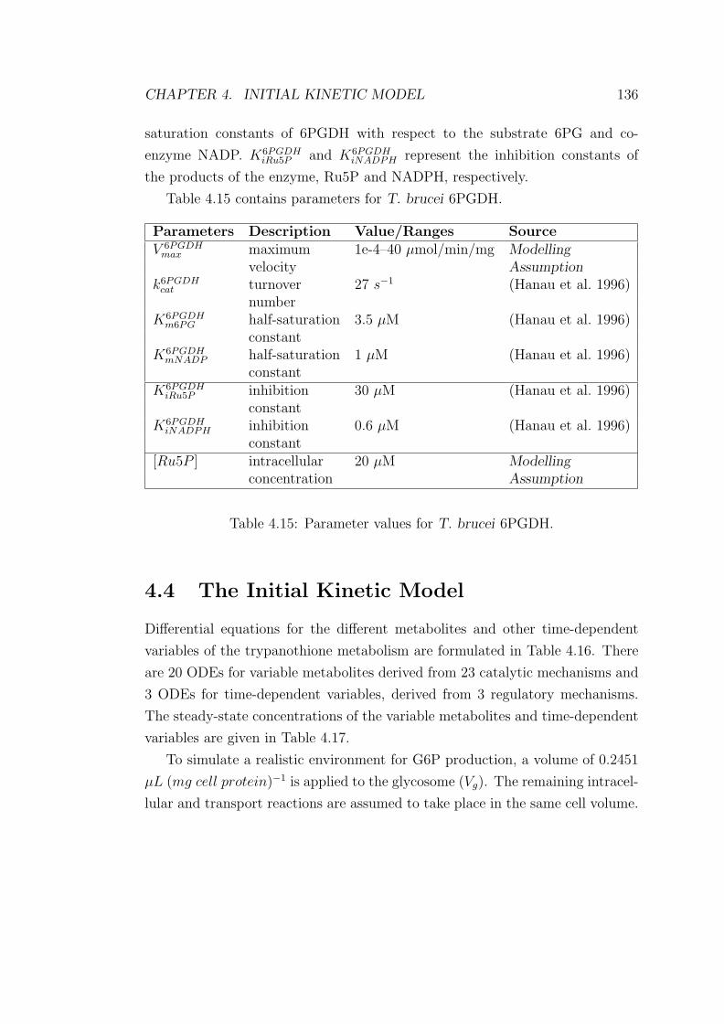
CHAPTER 6. MULTI-OBJECTIVE PSWARM 190
origin.
6.5.1 Archive Updating Strategies
Our in silico study also investigates how the choice of updating strategy for
the archive REP affects the performance of the algorithm when solving the
ERK signalling pathway. The strong-dominance updating strategy only allows
non-dominated particles to be inserted into the archive, which differs from the
weak-dominance updating strategy, where partially dominated particles are also
accepted.
In all the four variants of MoPSwarm (In Variant 1 to Variant 4 defined
above, the weak-dominance updating strategy was applied), the strong-dominance
updating strategy is adopted instead and the performance of each variant is ex-
amined. Interestingly, all these variants converged to a single solution at the
end of each run of the optimization (altogether there were 10 runs, each with
a different population of initial particles). Thus adopting the strong-dominance
updating strategy fails to maintain diversity in the non-dominated solutions.
According to the criteria used to assess the performance of multi-objective algo-
rithms, the weak-dominance updating strategy is preferable.
Figure 6.4 illustrates the potential problem with the strong-dominance up-
dating strategy. If there is a non-dominated solution PN (red filled square) found
in the later stages of the flying cycle, the Pareto-optimal front (black filled cir-
cles) developed in the earlier stages will be completely eliminated. This makes it
very difficult to re-form a well-distributed front again, rather the search engine
is more inclined to move towards the origin as shown by the arrow in red.
Based on the experimental results, we summarize that in the multi-objective
optimization scheme, the selection of global best guide and the update of ex-
ternal repository are two major problems that have to be addressed carefully.
An appropriate selection mechanism is critical in guiding the search towards
the Pareto-optimal set and achieving a well distributed trade-off front. We have
found that it is a very challenging problem particularly where multi-optimization
algorithms are proposed for solving real-world applications. Our in silico investi-
gation (Figure 6.3) demonstrates that the Crowding Distance computation and
the refresh step can facilitate the generation of a well-distributed and smooth
Pareto-optimal front.
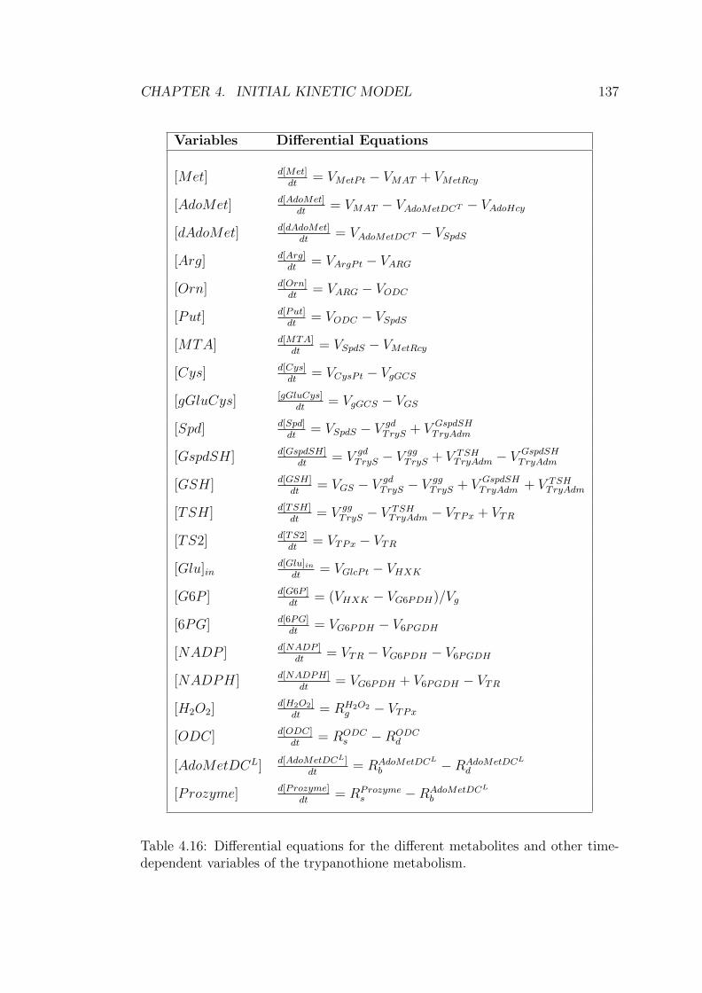
CHAPTER 6. MULTI-OBJECTIVE PSWARM 191
0 50 100 150 200Objective 1
0
100
200
300
400
500
600
700
Obj
ectiv
e 2
PN
Figure 6.4: An illustration of the strong-dominance updating strategy. Thesolution PN moves towards the origin indicated by red arrow.
6.5.2 Mutation Mechanism
Most of the existing implementations of multi-objective optimization with PSO
apply some sort of mutation operator (Reyes-Sierra and Coello 2006). The muta-
tion scheme adopted in the method designed by Coello et al. (Coello et al. 2004)
is implemented in MoPSwarm (Variant 4) and compared with the ‘vanilla’ algo-
rithm. The optimization results from the original MoPSwarm and MoPSwarm
with mutation are shown in Figure 6.5. The results were obtained using 10
particles and 20 iterations.
Our in silico investigations indicate that the mutation operator resulted in
inferior solutions, which is likely due to the additional disorder introduced into
the system by the operator, making it more difficult/slower to converge. As
explained in Figure 6.5, by the end of 20 iterations, MoPSwarm without the
mutation operator produces slightly better results than the alternative. By the
end of the search process (which stopped at 432 iterations due to single particle),
MoPSwarm without mutation produced a good, well-distributed Pareto-optimal
set, whereas MoPSwarm with mutation produced a solution set with much less
diversity, with the results being essentially a small subset of those produced

CHAPTER 6. MULTI-OBJECTIVE PSWARM 192
120 140 160 180 200Steady-state Condition
250
300
350
400
Pert
urbe
d C
ondi
tion
Without MutationWith Mutation
Figure 6.5: A comparison of the performance of MoPSwarm in the use of themutation operator by the end of 20 iterations of the search process.
by MoPSwarm without mutation. The mutation operator tends to drag the
search into a small and condensed area of the parameter space, giving rise to
convergence to a small set of similar solutions.
Reyes-Sierra and Coello (Reyes-Sierra and Coello 2006) draw attention to the
issue that the choice of a good mutation operator is a difficult task, and there
are approaches that show good performance without using any kind of mutation
operator. The incorporation of a mutation operator certainly deserves a more
careful study, which is beyond the scope of the thesis, however. The mutation
mechanism is excluded from our proposal according to the results from the in
silico investigations on the issue.
6.5.3 Optimization Results with MoPSwarm
The predicted concentration profiles of Raf1/RKIP, Raf1/RKIP/ERK, MEK-PP
and MEK-PP/ERK in both steady-state and perturbed conditions are generated
with two particular sets of parameters estimated with Variant 4 of MoPSwarm.
These two sets of parameters are selected from the upper-left end and bottom-
right end of the Pareto front, as shown in Figure 6.3(d).
CHAPTER 6. MULTI-OBJECTIVE PSWARM 193
Parameter Set 1:
k1 = 0.7885, k2 = 0.0576, k3 = 0.5600, k4 = 0.0044, k5 = 0.0218,
k6 = 0.3934, k7 = 0.0068, k8 = 0.0482, k9 = 0.7927, k10 = 0.0041, k11 = 0.7160.
m1|t=0 = 0.4110, m2|t=0 = 0.3200, m3|t=0 = 0.5178, m4|t=0 = 1.4004,
m5|t=0 = 0.0391, m6|t=0 = 0.0205, m7|t=0 = 1.6726, m8|t=0 = 0.8149,
m9|t=0 = 0.1718, m10|t=0 = 2.9295, m11|t=0 = 0.0554.
β = 0.2662.
Parameter Set 2:
k1 = 0.6527, k2 = 0.0106, k3 = 0.5399, k4 = 0.0039, k5 = 0.0330,
k6 = 0.3975, k7 = 0.0010, k8 = 0.0301, k9 = 0.8044, k10 = 0.0026, k11 = 0.7328.
m1|t=0 = 0.4115, m2|t=0 = 0.3198, m3|t=0 = 0.5081, m4|t=0 = 1.3980,
m5|t=0 = 0.0336, m6|t=0 = 0.0201, m7|t=0 = 1.8198, m8|t=0 = 0.8063,
m9|t=0 = 0.1767, m10|t=0 = 2.8189, m11|t=0 = 0.0549.
β = 0.2588.
Parameter Set 1 and Parameter Set 2 are the solutions that have the
minimum values for a single objective function across the Pareto-optimal set,
that is, they have the best objective function values for the steady-state and
perturbed conditions respectively. The steady-state and perturbed concentration
profiles predicted with Parameter Set 1 and Parameter Set 2 are shown in
Figure 6.6 & Figure 6.7 and Figure 6.8 & Figure 6.9, respectively. As indicated
previously, only the four system components shown here present responses to
knockdown of k8, thus the other system components are omitted. It should be
noted that this approach yielded good predictions of the dynamics of the other
system components.
The steady-state concentration profiles of the pathway are simulated with the
model given in Table 5.1 in Chapter 5. The perturbation profile of the pathway
is simulated with the model given in Table 6.1, where the initial condition cor-
responds to the concentration level of the system components simulated for the
steady-state condition. The true experimental data used for comparison against
the simulation results in both conditions is produced with the reference and per-
turbed (with a 90% knockdown applied to k8) parameter sets of the pathway,
respectively.

CHAPTER 6. MULTI-OBJECTIVE PSWARM 194
Compared to the simulation results using the conventional approach (shown
in Figure 6.2), predictions with our proposal are reasonably satisfactory for
both objectives given the large number of unknown parameters. The simulation
profiles shown in Figure 6.6 to Figure 6.9 indicate that with both parameter
sets, the model predicts a steady-state value close to the target, and can also
reproduce the measured dynamics of the system components, even though no
exact match is found in the optimization of either objective.
The predicted values of the perturbation, β, vary between 0.1 and 0.3 along
the Pareto front, which is comparable to the true perturbation value, β = 0.1.
From a biological point of view, predictions of the perturbation between 0.1 and
0.3 indicate that similar effects on the system dynamics could be achieved by
a lower degree of knockdown on the reaction enzyme of interest (i.e. a 70%–
80% predicted perturbation produces a similar effect to the true perturbation of
90%). This observation is useful in a general sense in that although the activity
of an enzyme can never be completely suppressed, enzymes that are easier to
suppress are preferable as drug targets (Bakker et al. 2002). Therefore, one of
the important applications of our proposal is to provide alternative solutions for
perturbation experiments where modifying the rate reaction constants (or initial
concentrations) is more economical and probable than designing a high-affinity
compound inhibitor.
6.6 Discussion
Given that the use of mathematical models may have large consequences for drug
development in case of model inadequacy or lack of precision, these models must
go through a rigorous validation process before they can be adopted as predictive
models. The use of a multi-objective optimization scheme is encouraged for
reliable model validation. It appears to be a natural solution to the optimization
problem that is constrained by more than one condition, particularly, in cases
where, among all the unknown parameters, a subset of parameters is common
to all the objectives and some of them are specific to certain objectives.
The proposed approach MoPSwarm is beneficial in tackling the systems
where the components are time-dependent variables and the number of unknown
parameters is large. MoPSwarm can successfully detect solutions exhibiting con-
vex tradeoffs in the objective function space using a smaller number of popu-
lation (20 initial particles) within a smaller number of generations (maximum

CHAPTER 6. MULTI-OBJECTIVE PSWARM 195
0 50 100 150 200Time (mins)
0
0.5
1
1.5
2
2.5
3C
once
ntra
tion
(Arb
. Uni
ts)
Figure 6.6: Comparison of the predicted concentration profile (continuous line)and the true steady-date data (segment line) for (filled circle): Raf1/RKIP,(open circle): Raf1/RKIP/ERK, (filled square): MEK-PP and (open square):MEK-PP/ERK. The predicted concentration profile is yielded with ParameterSet 1.
1000 generations). By applying the multi-objective optimization scheme, alter-
native solutions that are more practical and effective can be obtained for design
of perturbation experiments. Compared to biological experiments, computa-
tional study is an economical strategy, which can help biologists design in vivo
experiments in a more efficient way.
We presented a comparative study investigating some of the factors impor-
tant to the performance of MoPSwarm in solving multi-objective optimization
problems. We found that the choice of selection scheme for global best guide
and the mechanism for updating the archive is critical for the Pareto-based ap-
proach, from the perspective of promoting an effective search towards the Pareto
front and maintaining diversity in the population.
In summary, a multi-objective optimization scheme is advantageous over
single-objective optimization in two major aspects.
First, in the context of single-objective optimization, a multi-criteria fitness
value must be defined to aggregate individual fitness value, in order to perform

CHAPTER 6. MULTI-OBJECTIVE PSWARM 196
0 50 100Time (mins)
0.5
1
1.5
2C
once
ntra
tion
(Arb
. Uni
ts)
Figure 6.7: Comparison of the predicted concentration profile (continuous line)and the true perturbation data (segment line) for (filled circle): Raf1/RKIP,(open circle): Raf1/RKIP/ERK, (filled square): MEK-PP and (open square):MEK-PP/ERK. The predicted concentration profile is yielded with ParameterSet 1.
an optimization or search process with a single objective. This multi-criteria
fitness value summarizes the degree of satisfaction of all the individual criteria.
The danger of function aggregation lies in the fact that the objectives with large
values may dominate the search process. This leads to the result that objectives
with large function values could be satisfactorily optimized but the performance
of objectives with small function values is always poor. One way to solve the
problem is to weight the individual measures for each criteria and carefully com-
bine them all together into a single measure. However, in our experience, it is
not trivial to develop a good multi-criteria measure that aggregates the individ-
ual criteria properly, which may have a significant impact on the optimization
performance.
Second, in the context of single-objective optimization, normally only one
solution can be detected per optimization run. On the contrary, with the multi-
objective optimizer, a set of Pareto-optimal solutions can be obtained with a
single run of the algorithm. Considering all the objectives simultaneously but in

CHAPTER 6. MULTI-OBJECTIVE PSWARM 197
0 50 100 150 200Time (mins)
0
0.5
1
1.5
2
2.5
3C
once
ntra
tion
(Arb
. Uni
ts)
Figure 6.8: Comparison of the predicted concentration profile (continuous line)and the true steady-state data (segment line) for (filled circle): Raf1/RKIP,(open circle): Raf1/RKIP/ERK, (filled square): MEK-PP and (open square):MEK-PP/ERK. The predicted concentration profile is yielded with ParameterSet 2.
a separate form during the search process allows practitioners to favor certain
objectives over the others in the selection of solutions. Given the Pareto-optimal
front in Figure 6.3(d), biologists can choose the solution according to the impor-
tance ascribed to each objective. For example, if it is more important for the
objective concerning the perturbed condition to be accurately optimized, then
the solutions lying at the bottom of the front are favored, which are the ones
that hold smaller values for this objective function.
Further statistical analysis of the Pareto-optimal solutions of multi-objective
optimization problems can be carried out. Important information can be ob-
tained from the Pareto-optimal front with regards to the reliability of the esti-
mated parameters. This can be achieved by analyzing the variation of estimated
values of the unknown parameters along the Pareto-optimal front. If the esti-
mated values of one parameter vary widely, then it may indicate that either
the available experimental data is not informative enough or the model contains
intrinsic difficulties for estimating this parameter.

CHAPTER 6. MULTI-OBJECTIVE PSWARM 198
0 50 100Time (mins)
0.5
1
1.5
2C
once
ntra
tion
(Arb
. Uni
ts)
Figure 6.9: Comparison of the predicted concentration profile (continuous line)and the true perturbation data (segment line) for (filled circle): Raf1/RKIP,(open circle): Raf1/RKIP/ERK, (filled square): MEK-PP and (open square):MEK-PP/ERK. The predicted concentration profile is yielded with ParameterSet 2.
Application of the analysis (described above) to the solutions displayed in
Figure 6.3(d) implies that it may be hard for parameters k2 and k7 to be accu-
rately estimated with the given observed data, where the coefficient of variation
(ratio of standard deviation over mean) of the estimated values of these param-
eters is large: up to 0.5. Large variations shown on k2 and k7 suggest that
reactions involving these two parameters should ideally be further characterized
or/and more biological experiments concerning the pathway (i.e. with a focus on
the reactions containing k2 and k7) should be designed so as to obtain substantial
measurements.
In Chapter 7, a schematic approach for system identification of the trypan-
othione metabolic pathway in T. brucei is presented. MoPSwarm (Variant 4) is
applied to model validation of the polyamine biosynthetic sub-pathway.

Chapter 7
A Methodological Framework for
Mathematical Modelling of the
Trypanothione Metabolic
pathway
In this chapter we describe the challenges of computational modelling of complex
systems where prior knowledge about the system is incomplete and experimen-
tal data is sparse. We propose a methodological framework to address these
challenges and illustrate the feasibility of the approach in guiding our work on
the computational modelling of a real biological system – the trypanothione
metabolic pathway in Trypanosoma brucei.
7.1 The Challenge
Sauro et al. (Sauro et al. 2006) stated that, owing to the inherent non-linearity
of biological systems, the problem of system identification is extremely challeng-
ing. The authors drew attention to the biochemical network inverse problem
when there are many variables for which there is no experimental data and also
pointed out that few of the existing attempts have been applied to severely
under-determined problems where only a limited amount of information can
contribute to model construction.
Mechanistic modelling is a particularly useful tool in the study of new bio-
logical processes. However, despite its great value, the application of this type
199

CHAPTER 7. A PROPOSED METHODOLOGICAL FRAMEWORK 200
of modelling of large-scale complex biological systems is not straightforward
and sometimes impractical because it necessitates the consideration of many
pathways for which detailed reactions and their kinetic parameters are not yet
known. This is complicated by the fact that exact mechanisms accounting for
the phenomenon under study are frequently elusive.
The experimental measurements of the trypanothione metabolic pathway
are insufficient to achieve a complete mathematical description of the pathway.
In addition, there are several challenges to constructing a suitable mechanistic
mathematical model of the trypanothione pathway. First, there is uncertainty
in the network topology describing chemical activities of the relevant system
components. Second, the use of in vivo enzyme kinetics and regulatory data
measured from different experimental settings also poses difficulties. It is nec-
essary to explore both the model structure and missing parameters in order for
the identification of an appropriate model.
There are many challenges that are imposed on conventional approaches to
modelling, simulation and analysis by the complexity of biological pathways.
This is further complicated by data sparsity, which leads to a requirement for
novel approaches to cope with these challenges (van Riel 2006).
7.2 Goals and Objectives
As stated in Chapter 1, the intended use of the model has a critical impact on
the approaches applied at different stages of the modelling procedure. There
are two primary goals of our work on kinetic modelling of the trypanothione
metabolic pathway as follows:
1. Given the mathematical formulation combined with the estimated param-
eters, the model can reproduce the observed biological phenomenon.
2. With a valid model, predictions of the system responses under different
experimental conditions can be obtained and hypotheses regarding the
biological pathway can be generated to be proved or disproved experimen-
tally.
In order to achieve these goals, two categories of mathematical models are
required for the pathway under consideration – a descriptive model and a predic-
tive model. Different computational strategies are recommended to accomplish
the specific objectives.

CHAPTER 7. A PROPOSED METHODOLOGICAL FRAMEWORK 201
Descriptive models are concerned with the question of ‘whether the model
can reproduce the experimentally measured dynamics of the system’. One use of
such models is to estimate the unknown kinetic parameters and the structural
characters of the system in silico. Descriptive models are evaluated in terms
of goodness of fit and finding a good fit involves simultaneously exploring the
mathematical structure and unknown parameters. The compatibility of simula-
tion results with experimental data provides evidence for the credibility of the
model.
Predictive models are concerned with the question of ‘does the model ade-
quately describe the system of interest’. In other words, in addition to repro-
ducing biological observations, models must be developed to allow predictions
of system dynamics in response to environmental or genetic perturbations. Pre-
dictive models are usually validated using independent data that is not used
for model building and parameter estimation. Good predictions of independent
data can be used to assess the applicability of the model.
7.3 Our Approach
The challenge of kinetic modelling of complex biological systems is investigated,
when prior knowledge about the system is incomplete and observed data is
sparse. We develop a methodological framework to tackle the challenge and
assess the usefulness of our proposal on the trypanothione metabolic pathway.
The schematic flowchart of the proposed methodological framework is illus-
trated in Figure 7.1. The major phases of this framework are Initial Model
Construction, Model Decomposition, Model Reconstruction and Model Valida-
tion. The Model Structure Exploration step is employed in the phases of model
decomposition and model reconstruction, where necessary and applicable. The
proposed framework can be generalized to mathematical modelling of any non-
linear systems that are at best characterized with incomplete and sparse obser-
vation data.
One big strength of this framework is that it can be applied to tackle the
system identification problem of different sub-systems in an independent man-
ner. Once biological information is sufficient for the in silico investigation, these
sub-systems can be further studied with regard to the correctness of mathe-
matical model structures and unknown parameters can be estimated. After the
remaining unexplored portion of the pathway is successfully resolved, the final

CHAPTER 7. A PROPOSED METHODOLOGICAL FRAMEWORK 202
Simulate Initial Model
Decomposition
Decompose Model
Compare with Experiment
Optimization-based Simulation
Model StructureExploration
Reconstruction
Add Removed External Reactions
Optimization-based Simulation
Initia
mpos
struc
No
Yes
Yes
No
Targeted BiologicalExperiments
No Yes
No
Model Validation
Black Box Approximationof Inputs/Outputs (if applicable)
MoPSwarm
No
Yes
Refine Model
Final Model
NoRefine MoFurther Iterations
of This Approach
Yes
Y
oN
SatisfactoryResults?
Initial Model Construction
Model StructureExploration
NoNo
No
Yes
Model StructureExplorationSuccessful?
Yes
No d Bio
Model(s) of OtherSub-systems
Merge Models(if applicable)
y
YYYYes
Correct ModelStructure?
Correct ModelStructure?
YesDecompose Further?
YesYYYYe
SatisfactoryResults?
l Mo
Figure 7.1: The schematic flowchart of the proposed methodological framework.
model of the trypanothione metabolic pathway can be developed by integrating
the models describing individual sub-systems in the step of Merge Model. If
the models are not directly connected, then black-box connectors are required
to link the models and the involved parameters have to be estimated.

CHAPTER 7. A PROPOSED METHODOLOGICAL FRAMEWORK 203
The phase of Initial Model Construction involves gleaning prior knowledge of
the system from the literature, including identifying the network topology, the
characters of enzymatic-reaction mechanisms and the experimentally measured
initial states. The initial states, in the context of biological systems, refer to the
initial concentrations of the system components and kinetic parameter values of
the enzyme catalyzed reactions. The initial kinetic model of the trypanothione
metabolic pathway was presented in Chapter 4.
The phase of Model Decomposition aims to decompose the initial system
into functionally independent sub-systems, and study structural insufficiency
via optimization-based simulation. Models of each sub-system are represented as
closed systems, where the inputs and outputs of the sub-systems are known vari-
ables, approximated with the measured dynamics from biological experiments.
The degree of decomposition is dependent on the correctness of mathematical
model structures of the sub-systems and the availability of experimental mea-
surements for system components. Choosing a model variable to initialize the
decompositional process is not a trivial task. We take advantage of the struc-
tural modelling (see Chapter 3) as a strategy to determine the initial functional
sub-system(s). In this phase, mathematical structures of the sub-systems are
examined and the structures are rejected if no satisfactory fit with the experi-
mental data can be obtained for any possible set in the parameter space. The
consistency of the model behaviour is verified through a qualitative comparison
with experimental data.
The phase of Model Reconstruction continues the investigation into the cor-
rectness of mathematical model structures, the appropriateness of which is ex-
amined via the same optimization procedure. Model reconstruction is an itera-
tive procedure, which can be understood as the reverse of model decomposition,
where enzymatic reactions may be added and/or removed from the sub-system.
By the end of this phase, structurally-correct models can be identified that allow
mechanistic insights into the system or sub-systems, and useful in vivo experi-
ments can be suggested in order to enable structural exploration of the remaining
portions of the system (if there are any) in the future.
Sub-system models that are obtained from the model decomposition and/or
reconstruction phases may be structurally incorrect. Candidate models for these
sub-system(s) are examined for appropriateness in the Model Structure Explo-
ration step. Detailed biological information on structural constraints of the sub-
system is required in order to design biologically meaningful model variants. The

CHAPTER 7. A PROPOSED METHODOLOGICAL FRAMEWORK 204
structural constraints can be specified using the network topology (i.e. elemen-
tary reaction steps) and/or the kinetic character (i.e. regulatory mechanisms
of enzymes or between enzymes). When it is feasible, the constraints are incor-
porated into the current mathematical structure of the sub-system to formulate
new model structures and the appropriateness evaluated via optimization-based
simulation. If a candidate mathematical structure reproduces experimental data
sufficiently accurately, then according to Heinrich et al. (Heinrich et al. 1977),
it is likely that this sub-system is correctly modelled.
The phase of Model Validation is concerned with proving that the model is an
adequate representation of reality, which gives confidence that the model is useful
not only for reproducing measured dynamics, but also consistently interpreting
the underlying biological processes. The multi-objective optimization algorithm,
MoPSwarm, proposed in Chapter 6 is applied in this phase. If only structurally-
correct sub-system(s), rather than a complete kinetic model, are obtained from
the previous phases, then a black-box approximation must be applied to the
inputs and/or outputs of the sub-system(s) prior to the validation procedure
in order to render predictive power. The applicability of the model with the
parameter estimates solved using MoPSwarm is assessed by comparisons between
the model predictions and independent data sets obtained from distinct states of
the system. We term the data sets serving as the inputs to MoPSwarm algorithm
as Estimation Data and the independent data sets for model assessment as
Validation Data. Unsatisfactory results trigger the model refinement process,
which may involve checking the reliability of validation data or examining the
presence of regulatory mechanisms that may be missing from the model.
According to the conventional process of in silico simulation, the model
should be solved as a whole, with all the parameters estimated simultaneously
using the optimization method. The missing protein initial concentrations are
treated as parameters to be estimated together with the unknown kinetic pa-
rameters. The initial kinetic model of the trypanothione metabolism proposed
in Chapter 4 (see Section 4.4) consists of 23 ODEs derived from 23 catalytic
mechanisms and 3 regulatory mechanisms. In this thesis, we focus on study-
ing the trypanothione dynamics at the metabolic level. Towards the end, only
ODEs for variable metabolites are taken into consideration, which results in a
kinetic model consisting of 23 catalytic mechanisms with 80 kinetic parameters.
There are 29 unknown kinetic parameters to be estimated with the optimiza-
tion method and 3 unknown initial concentrations (intracellular AdoHcy, cys-

CHAPTER 7. A PROPOSED METHODOLOGICAL FRAMEWORK 205
teine and G6P). According to Chapter 4, the initial concentration of AdoHcy
can be approximated from the metabolite AdoMet with the equality constraint
[AdoHcy] = 0.2 × [AdoMet].
Prior to computational simulation, models may be simplified by reducing the
number of unknown parameters so as to improve the performance of system iden-
tification. Based on relevant qualitative knowledge, meaningful simplifications
can be introduced on two unknown kinetic parameters as follows.
First, AdoMetDC is assumed to be present in the cell in two forms, namely a
free form and a ligand-occupied form. The total concentration of AdoMetDC is
therefore the superposition of free-form AdoMetDC and ligand-occupied AdoMe-
tDC. We introduced a factor β to represent the percent of free-form AdoMetDC
taking up the total enzyme concentration, thus the ligand-occupied form is ex-
pressed as 1 − β of the total concentration. Willert and Phillips (Willert and
Phillips 2008) observed that the prozyme reacting with AdoMetDC is a lim-
iting factor on the activity of AdoMetDC. This observation implies that the
concentration of the ligand-occupied form accounts for a limited quantity of the
total AdoMetDC concentration. β is assumed to vary between 0.5 and 1 in or-
der to reflect the experimental observation and still allow the ligand-occupied
AdoMetDC to change within a physiologically feasible range. In this way, the
three unknown parameters are reduced to two unknown parameters – the total
concentration of AdoMetDC and the ratio β. The mathematical rate expressions
of the ligand-occupied and free form of the enzyme defined in Equation (4.6) and
Equation (4.7) in Chapter 4 are modified to the following equations
VAdoMetDCL = kAdoProcat · [AdoMetDCT ] · (1 − β) ·
[AdoMet]
KAdoPromAdoMet
1 +[AdoMet]
KAdoPromAdoMet
(7.1)
VAdoMetDCO = kAdoMetDCO
cat · [AdoMetDCT ] · β · (7.2)
[AdoMet]
KAdoMetDCO
mAdoMet
1 +[AdoMet]
KAdoMetDCO
mAdoMet
+[dAdoMet]
KAdoMetDCO
idAdoMet
+[KAdoMetDCO
aPut ]
[Put]
Second, a relation between the enzyme activities of trypanothione peroxidase,
V TPxmax , and H2O2 synthesis rate, Rsyn, is approximated. The published values

CHAPTER 7. A PROPOSED METHODOLOGICAL FRAMEWORK 206
for V TPxmax and Rsyn have been extracted from the literature, which are 1.3 nmol ·
min−1 ·(108 cells)−1 and between 0.2–0.7 nmol ·min−1 ·(108 cells)−1, as given in
Chapter 4. We clarified that the standard unit of enzyme specificity is defined as
μmol ·min−1 · (mg of cells)−1. However, both values are given in the literature
in a different unit. To transform the values into the standard enzyme unit,
the protein concentrations of the associated enzymes must be known. There
are, unfortunately, difficult to measure in vivo. Instead, with the published
values in units of number of cells, a ratio of V TPxmax and Rsyn can be derived,
which falls in the range 1.8 to 6.5. In our study, a ratio of 6.5 is assumed
to describe the relationship between the two parameters, thus removing one
unknown parameter.
7.4 Initial Model Simulation
The experimental observations adopted for global optimization were obtained
from the paper by Fairlamb et al. (Fairlamb et al. 1987). The reported data set
describes the in vivo drug-induced dynamics of bloodstream-form T. brucei in
response to DFMO. This is the only relevant data source that was obtainable for
this project. A few of other types of data has been published (e.g. gene knock-
down data), but they are comparatively insufficient to be used as the Estimation
Data for the identification of model structure and unknown parameters.
The experimental measurements published by Fairlamb et al. are available
for eight metabolites, namely AdoMet, dAdoMet, ornithine, putrescine, spermi-
dine, glutathione, GspdSH and trypanothione, with data given for three time
points (12 hrs, 36 hrs and 48 hrs). This results in a partial and sparse opti-
mization problem, where the availability of observed data is given for only a
portion of the total metabolites (8 out of 20 metabolites) and measured at a
limited number of time points. This constraint poses a significant challenge to
the optimization problem under study.
In order to apply the drug perturbation data reported by Fairlamb et al., a
modification to the initial model has to be modified by incorporating the DFMO-
induced factors. DFMO profoundly changes the metabolism of T. brucei by
altering the enzyme activity of ODC, in consequence, influencing the polyamine
synthesis and content. The steady-state protein levels of other enzymes, in-
cluding SpdS, AdoMetDC, γ-GCS, prozyme, TryS and TR were unaffected by
DFMO inhibition (Xiao et al. 2009).

CHAPTER 7. A PROPOSED METHODOLOGICAL FRAMEWORK 207
According to Bacchi et al. (Bacchi et al. 1983), ODC activity was decreased
by more than 99% within 12-hour treatment of DFMO. In our study, the generic
form of enzyme activity is represented as the product of turnover number and
the protein concentration
V ODCmax = kODC
cat · [ODC] (7.3)
where kODCcat remains fixed in all conditions but the enzyme concentration, [ODC],
may vary in some cases when the biological system is treated with an activator
or inhibitor.
To describe the enzyme inhibition, time-dependent changes of the ODC con-
centration in response to DFMO have to be explicitly modelled. The inhibition
is assumed to follow an exponential decay, expressed as
[ODC]ss · e−λ·t (7.4)
where [ODC]ss is the steady-state ODC concentration. Parameter λ is solved
for simple curve fitting using the qualitative description of the enzyme dynamics
with addition of DFMO and takes a value of 0.007 in this instance. A detailed
discussion of this drug-enzyme interaction was given in Section 4.3.1 in Chap-
ter 4. The rate equation of the enzyme under normal conditions, which was
defined in Equation 4.2, is modified to give the following:
VODC = kODCcat · [ODC]ss · e−λ·t ·
[Orn]
KODCmOrn
1 +[Orn]
KODCmOrn
+[Put]
KODCiP
(7.5)
No boundary values for the unknown parameters can be directly extracted
from the literature. In terms of optimization, there is a trade-off between small
and large ranges within which the parameters may vary. Small ranges on un-
known parameters lead to a narrow search space that will probably preclude po-
tentially good solutions from consideration. On the other hand, a broad search
space is more likely to lead to globally optimal solutions by thoroughly explor-
ing the search space. However, in the latter case it is more likely that the
optimization will move into a region of the search space where the ODE solver
becomes numerically unstable. The lower and upper bounds imposed on the
unknown parameters were assumed to be based on the modeller’s experiences

CHAPTER 7. A PROPOSED METHODOLOGICAL FRAMEWORK 208
and communications with the biologists. The boundary values are reported in
Chapter 4 and are deemed appropriate for the current study. The possibility
that the model is not soluble is thus less likely to stem from ill formation of the
parameter search space.
In total, we carried out 300 optimization runs using the global optimization
algorithm PSwarm. The algorithm parameters were set as follows: 50 initial
particles in the population, 2000 maximum iteration number and 5000 maximum
function evaluations. The simulations were performed for 48 hours and the model
was solved using ode15s from Matlab.
The optimization method failed to produce a set of parameters that can
reasonably reproduce the experimental data. Figure 7.2 shows the simulation
results and experimental measurements for the metabolites critical to the reg-
ulation of trypanosomal growth, including spermidine, glutathione-spermidine
conjugate and trypanothione. The simulation results were calculated with the
estimated set of parameters having the smallest objective function value. In
Figure 7.2(a), Figure 7.2(b) and Figure 7.2(c), the simulation results are con-
stantly higher or lower than the observed data, representing distinct dynamic
trends over the time course. Figure 7.2(d) shows interesting dynamics, where the
simulation results are both higher and lower than the observed data at different
time points.
The optimization problem under investigation is a non-linear, high dimen-
sional problem. Simultaneously estimating all the unknown parameters in the
pathway is computationally expensive and sometimes not possible. This is par-
ticularly true when the observed data is limited. The problem is further com-
plicated by correlations between the unknown parameters. In the following sec-
tions, the proposed methodological framework is applied to guide the computa-
tional modelling of the trypanothione metabolic pathway. We aim at exploring
the ill-defined kinetic mechanisms of the reactions, subsequently, inferring po-
tentially suitable structures, and identifying the sub-system for which a sound
mathematical model can be possibly obtained given the limited experimental
data.
7.5 Model Decomposition
Cells can be seen as composed of a number of sub-systems. These sub-systems
themselves can in turn be further broken down into sub-systems — for example,

CHAPTER 7. A PROPOSED METHODOLOGICAL FRAMEWORK 209
0 500 1000 1500 2000 2500 3000Time (min)
1
10
100
log
GSH
Con
c. (μ
M)
Simulation DataObserved Values
(a) glutathione
0 500 1000 1500 2000 2500 3000Time (min)
0
500
1000
1500
2000
2500
3000
3500
Spd
Con
c. (μ
M)
Simulation DataObserved Values
(b) spermidine
0 500 1000 1500 2000 2500 3000Time (min)
20
30
40
50
60
70
80
90
100
Gsp
dSH
Con
c. (μ
M)
Simulation DataObserved Values
(c) GspdSH
0 500 1000 1500 2000 2500 3000Time (min)
0
500
1000
TSH
Con
c. (μ
M)
Simulation DataObserved Values
(d) trypanothione
Figure 7.2: Simulation profiles compared to experimental data for the keymetabolites when solving the model as a whole. Logarithmic axis is used forglutathione in order to better present the data. Error bars are presented whereappropriate data was available in the original papers.
functionally independent modules. Biological systems can thus be seen as hier-
archical systems. As stated in Chapter 1, a key problem is how to functionally
modularize a system.
In this study, we propose a decompositional approach to break down the ini-
tial model, which is not well-characterized, into modules for the investigation of
the correctness of mathematical model structures. Each module fulfills a certain
metabolic function pertinent to the trypanothione metabolism. The boundaries
of each module are formed by the model components for which there are con-
centration profiles with experimental data. We term these model components as
constant components. Modules should be able to operate independently of the
rest of the system. In the context of global optimization, parameters included in
modules can be estimated separately from the remaining unknown parameters.
The proposed procedure for Model Decomposition is embodied in the follow-

CHAPTER 7. A PROPOSED METHODOLOGICAL FRAMEWORK 210
ing basic steps:
Step 1: If this is the first iteration, identify the initial point for model
decomposition to derive initial modules and go to Step 3. Otherwise,
go to Step 2.
Step 2: Remove boundary components of the module derived from the
previous step of model decomposition. The removal of boundary compo-
nents involves deleting the associated chemical reactions. The formation
of new boundaries should comply with the following conditions:
• If observed data is not available for the new boundary component
after the first set of boundary components is removed, then the re-
actions associated with this component must also be deleted. This
process may be continued for a number of iterations until the exte-
rior components of the resulting module are constant components.
• If observed data is available for the new boundary component af-
ter the first set of boundary components is removed, then either
the reaction(s) incoming to, or the reaction(s) outgoing from this
component are deleted, depending on whether the component set
participates in the module as an input or output.
Step 3: apply global optimization to the module obtained from the first
step. If the results are satisfactory when compared with experimental
results, then this module is considered as an ‘elementary’ module (the
module is assumed to be well-characterized) and no further decomposi-
tion is required.
Step 4: (optionally) return to the first step if the optimization results
are not satisfactory until the end point of decomposition is reached.
The proposed decompositional approach is an iterative process, the termi-
nation of which depends on the quality of the optimization results in describing
the measured system dynamics. Modules derived using this approach should
satisfy the following condition: boundary components of the module are treated
as independent inputs and only the components within the module are variable
components with dynamics dependent on time and the inputs. In order to ap-
ply the global optimization method to the modules, an additional constraint is
imposed – observed data should be available for at least one variable component

CHAPTER 7. A PROPOSED METHODOLOGICAL FRAMEWORK 211
contained in the module. The availability of observed data (e.g. coverage and
adequacy) therefore also determines the degree of model decomposition.
In order to check whether the module’s behaviour is consistent with experi-
mental data, the behaviour is qualitatively compared based on the similarity of
curves or on certain effects which the model can reproduce. This comparison
method is defined by Heinrich et al. (Heinrich et al. 1977) as ‘qualitative com-
parison’. The mathematical structure of the module is rejected if no satisfactory
fit with the experimental data can be obtained.
Identifying the first component to initialise model decomposition is a non-
trivial task, particularly for real systems, where the number of variable com-
ponents involved is often large. It is noteworthy that in metabolic networks a
potential relationship exists between topological modularity and the functional
classification of different metabolites, for example in the metabolic network of
E. coli (Ravasz et al. 2002).
We attempt to take advantage of the network hierarchy to guide the se-
lection of starting point for the decompositional procedure. In Chapter 3, we
conducted structural modelling of the trypanothione pathway. The results pre-
sented indicate that, from a topological perspective, trypanothione metabolism
is organized in a hierarchical architecture. This provides a natural breakdown of
the pathway into two large modules, responsible for two necessary components
of trypanothione metabolism, namely trypanothione biosynthesis and oxidative
stress defense.
However, the oxidative stress defense module cannot be processed for model
decomposition. As stated previously, there must be at least one variable com-
ponent contained in the module where observed data is available; however no
components contained in this module were provided in the experimental mea-
surements by Fairlamb et al..
There is however comparatively sufficient data to investigate the correctness
of the mathematical model structure of the trypanothione biosynthesis mod-
ule. Initially, the constant boundary components of this module are exogenous
methionine, arginine, cysteine and intracellular trypanothione. Following opti-
mization to assess the compatibility of the module with experimental data, the
module will be further partitioned into smaller but more integrated sub-modules.
The time evolution of the intracellular trypanothione is approximated with
a time-dependent polynomial. The use of different input functions to simulate
the concentration profiles of the boundary components has been found to have

CHAPTER 7. A PROPOSED METHODOLOGICAL FRAMEWORK 212
an impact on the accuracy of parameter estimation (Faller et al. 2003). With
the four data points (including the initial concentration) measured by Fairlamb
et al., a polynomial input function up to 4th order can be generated. In this
stage, the error in parameter estimates is irrelevant, since the comparison of
the module’s behaviour to the experimental data is qualitative rather than a
goodness-of-fit criterion, such as on the sum of least squares. A 3rd-order poly-
nomial function is employed in this case, which is believed to be sufficient the
qualitative comparison.
The first three stages of model decomposition of the trypanothione biosyn-
thesis sub-system are shown in Figure 7.3.
Model Decomposition–Stage 1 Optimization of the trypanothione biosyn-
thesis sub-system, which is shown Figure 7.3(A), failed to produce a satisfactory
match with the experimental data. In particular, simulation results for glu-
tathione, spermidine and GspdSH are no better than the results obtained by
solving the entire model (shown in Figure 7.2).
According to the decompositional rules, the trypanothione biosynthesis sub-
system is further decomposed by removing the boundary component, trypan-
othione, which involves deleting the incoming reactions of this metabolite. This
process results in a new module with GspdSH and glutathione as the boundary
components, shown in Figure 7.3(B). The results of this new module are however
still not compatible with experimental data. This indicates that a further level
of model decomposition is required in order to correct the module.
It is worth pointing out that setting glutathione as a known input results
in the optimization method being unable to correctly tune the parameters in-
volved in the upstream glutathione production reactions (sub-pathway in grey
in Figure 7.3(B)). This involves the reactions catalyzed by exogenous cysteine
transporter, gGCS and GS.
Model Decomposition–Stage 2 Removing the boundary component GspdSH
and associated reactions from the module (Figure 7.3(B)) leads to two individual
sub-pathways with spermidine and glutathione as the end products. As discussed
above, the glutathione production sub-pathway cannot be examined for mathe-
matical structure deficiency by parameter estimation because no observed data
is available for the intermediate components included in this sub-pathway.
The spermidine biosynthesis module, shown in Figure 7.3(C), is suitable

CHAPTER 7. A PROPOSED METHODOLOGICAL FRAMEWORK 213
Stage 1
Stage 2
Stage 3
A
B C
D
Figure 7.3: The first three stages of model decomposition of the trypanothionebiosynthesis sub-system: (top left): overview of the trypanothione biosynthesissub-network; (bottom left): reduced module of the sub-network via stage 1; (bot-tom right) reduced module of the sub-network via stage 2; (top right); reducedmodule of sub-network via stage 3. Boundary components of the three reducedmodules are denoted in brown color: GspdSH and glutathione in bottom left;spermidine in bottom right; and spermidine and ornithine in top right.
for the investigation of the correctness of mathematical model structure. In
this case, intracellular spermidine becomes the boundary component that is
approximated with a 3rd-order polynomial function. The simulation results
of the ‘known’ intermediate components (for which observed data is available)
including AdoMet, dAdoMet, ornithine and putrescine are shown in Figure 7.4.
Inspection of Figure 7.4 shows that a moderate improvement in the opti-

CHAPTER 7. A PROPOSED METHODOLOGICAL FRAMEWORK 214
0 500 1000 1500 2000 2500 3000Time (min)
0
500
1000
1500
2000
Ado
Met
Con
c. (μ
M)
Simulation DataObserved Values
(a) AdoMet
0 500 1000 1500 2000 2500 3000Time (min)
0
200
400
600
800
1000
1200
dAdo
Met
Con
c. (μ
M)
Simulation DataObserved Values
(b) dAdoMet
0 500 1000 1500 2000 2500 3000Time (min)
0
200
400
600
800
1000
Orn
Con
c. (μ
M)
Simulation DataObserved Values
(c) ornithine
0 500 1000 1500 2000 2500 3000Time (min)
0
100
200
300
400
500
600
Put C
onc.
(μ
M)
Simulation DataObserved Values
(d) putrescine
Figure 7.4: Simulation profiles compared to experimental data for the keymetabolites obtained in Stage 2 of the model decomposition. Error bars arepresented where appropriate data was available in the original papers.
mization performance in solving the spermidine biosynthesis module. Of the
four intermediate metabolites, the match with experimental data for dAdoMet,
ornithine and putrescine (Figure 7.4(b), Figure 7.4(c) and Figure 7.4(d)) is sat-
isfactory given the sparse experimental data. The simulation results of AdoMet
(Figure 7.4(a)) still contradict the target data in terms of the trend in the change
of transient concentrations.
The simulation profile of arginine is shown in Figure 7.5. No values were
reported by Fairlamb et al. for arginine concentrations in the DFMO inhibi-
tion experiment; however, its intracellular level is assumed not to significantly
change during the course of drug inhibition (Alan H. Fairlamb, personal email,
28 August 2007). Different arginine dynamics were observed in the procyclic-
form T. brucei by Bellofatto et al. (Bellofatto et al. 1987) (see Table A.2 in
Appendix A), where arginine concentrations were increased up to four times of
the steady-state level after 48 hours of DFMO treatment.
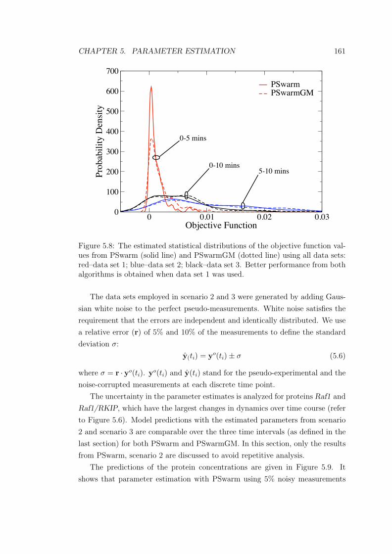
CHAPTER 7. A PROPOSED METHODOLOGICAL FRAMEWORK 215
0 500 1000 1500 2000 2500 3000Time (min)
0
200
400
600
800
Arg
Con
c. (μ
M)
Simulation Data
Figure 7.5: Simulation profiles for the arginine dynamics obtained in Stage 2of the model decomposition. Arginine concentrations reduced to 90% of thesteady-state level within 12 hours of DFMO treatment. No experimental datais available for arginine dynamics.
Regardless of which arginine dynamics are taken into account, simulation
results of the mathematical model deviate from experimental measurements. As
displayed in Figure 7.5, the model prediction for arginine concentrations are con-
tradictory to both assumptions that the concentration increases approximately
linearly or is unchanged during the course of DFMO treatment.
Model Decomposition–Stage 3 The unsatisfactory optimization results ob-
tained from Stage 2 promote further decomposition in order to identify possible
missing reactions or ill-defined kinetics of the spermidine biosynthesis module.
Since the number of metabolites for which observed data is available is compara-
tively large in quantity (4 out of 7 metabolites have experimental measurements),
the proposed decompositional approach allows several strategies to be developed
for decomposition of this module.
We take advantage of the optimization results obtained in Stage 2 to guide
the model decomposition in the current stage. Figure 7.4(a) and Figure 7.5
indicate that the dynamics predicted for AdoMet and arginine present differing

CHAPTER 7. A PROPOSED METHODOLOGICAL FRAMEWORK 216
trends to the observed data. This implies that the reactions participating in the
metabolism of AdoMet and arginine may be ill-characterized. As a consequence,
the purpose of model decomposition in this stage is to examine the correctness
of mathematical model descriptions of the related reactions. Two strategies can
be developed in accordance with the focus of investigation centered on either
AdoMet and arginine metabolism.
Strategy 1 with focus on AdoMet metabolism When the focus of in-
vestigation is concerned with AdoMet metabolism, the spermidine biosynthesis
module (Figure 7.3(C)) is decomposed by removing the upstream reactions for
ornithine production. Such decomposition leads to intracellular ornithine as the
new boundary component of the derived module, shown in Figure 7.3(D). The
concentration profile of intracellular ornithine is approximated with a 3rd-order
polynomial function.
The simulation results of the intermediate components including AdoMet,
dAdoMet and putrescine are shown in Figure 7.6.
It is clear that the simulation results for AdoMet, dAdoMet and putrescine
do not differ considerably from those obtained in Stage 2 of the model decom-
position. Apart from AdoMet (Figure 7.6(a)), the simulation results obtained
for dAdoMet and putrescine (Figure 7.6(b) and Figure 7.6(c)) via global opti-
mization are reasonably good, although not perfect. The overall optimization
performance is satisfactory for solving the high-dimensional search space, given
the limited and incomplete experimental data.
Simulation results in Figure 7.4(a) and Figure 7.6(a) show that almost no
difference is observed in the AdoMet dynamics. The intracellular concentra-
tions of AdoMet are estimated to remain constant over 12 to 48 hours after
DFMO inhibition. This is in contrast to the experimental observations from
Bacchi et al. (Bacchi et al. 1983) and Fairlamb et al. (Fairlamb et al. 1987)
that report AdoMet concentrations increasing more than 50 fold 48 hours af-
ter DFMO treatment. However, more recent and reliable biological experiments
(Xiao et al. 2009) support our model predictions that AdoMet concentrations do
not significantly change in response to DFMO treatment. This is not shown in
Figure 7.6 as Xiao et al. report only a qualitative comparison with their control
experiment.

CHAPTER 7. A PROPOSED METHODOLOGICAL FRAMEWORK 217
0 500 1000 1500 2000 2500 3000Time (min)
0
500
1000
1500
2000
Ado
Met
Con
c. (μ
M)
Simulation DataObserved Values
(a) AdoMet
0 500 1000 1500 2000 2500 3000Time (min)
0
200
400
600
800
1000
1200
dAdo
Met
Con
c. (μ
M)
Simulation DataObserved Values
(b) dAdoMet
0 500 1000 1500 2000 2500 3000Time (min)
0
100
200
300
400
500
600
Put C
onc.
(μ
M)
Simulation DataObserved Values
(c) putrescine
Figure 7.6: Simulation profiles compared to experimental data for the keymetabolites obtained in Stage 3 of the model decomposition. Ornithine is aninput. Error bars are presented where appropriate data was available in theoriginal papers.
Strategy 2 with focus on arginine metabolism When the focus of in-
vestigation is concerned with arginine metabolism, the spermidine biosynthe-
sis module is decomposed by removing the intracellular spermidine and by-
product MTA. This leads to the deletion of methionine and the related reac-
tions. AdoMet, dAdoMet and putrescine therefore become the new boundary
components, as shown in Figure 7.7.
Figure 7.7 shows that the arginine and dAdoMet biosynthetic sub-pathways
are topologically isolated and can be studied independently from each other, as
no interactions between the two branches are indicated at the metabolic level.
We are aware that changes in AdoMetDC activity have an impact on the gene
expression level of ODC (Willert and Phillips 2008), and that ODC suppression
may also have a concomitant influence on AdoMetDC activity, though this has
not yet been evidenced.
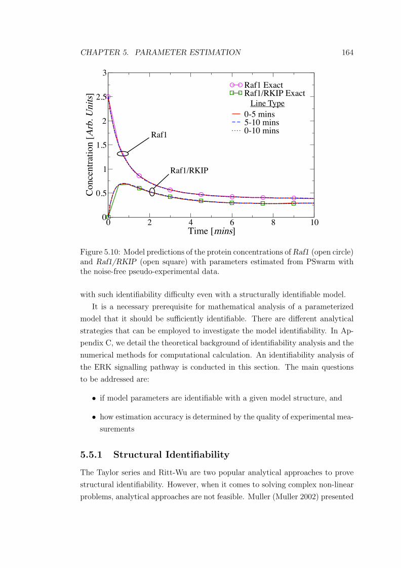
CHAPTER 7. A PROPOSED METHODOLOGICAL FRAMEWORK 218
Figure 7.7: Results of decompositional Stage 3, arginine-centered strategy
The gene-level regulation between the enzyme activities of AdoMetDC and
ODC is not considered in the phase of mode structure exploration, rather they
are solved independently from each other during the optimization process. This
consideration is consistent with the purpose of the current study, which aims to
seek possible solution(s) for the unknown parameters within the defined search
space so that model predictions are compatible with the measured dynamics of
the system. Elucidating the underlying relation between the enzyme activities of
AdoMetDC and ODC is not possible with the DFMO-induced data set that de-
scribes the changes in concentrations at the metabolic level, thus is not relevant
to this study.
The module used for investigating the correctness of the model of arginine
metabolism is the individual sub-pathway on the right side of Figure 7.7. This
module takes putrescine as the boundary component and employes a 3rd-order
polynomial function to approximate its concentration profile. No significant
improvements were obtained for the simulation results of arginine dynamics.
This implies that the enzymatic reactions concerning arginine dynamics may be
incorrect, which suggests in silico exploration for appropriate model structures.

CHAPTER 7. A PROPOSED METHODOLOGICAL FRAMEWORK 219
7.6 Model Structure Exploration
When one attempts to construct a novel model of a complex biological system,
for which the prior knowledge is partial, the first and foremost thing to do is to
examine the soundness of the mathematical model. The mathematical models
considered in this thesis are defined as a set of differential equations, which
associate the changes in concentration levels of system components with reaction
rate equations. The reaction rate equations express the enzyme reaction rate
as a function of the concentrations of other model components. The algebraic
expression for each rate equation depends on the kinetics under consideration.
In this thesis, we apply the law of Michaelis-Menten to model the biological
system of interest.
The structure of mathematical models can be characterized with two types
of structural constraints, including network topology and kinetic character. The
former refers to the spatial layout of system components and the reversibility
of the chemical conversion between them. The latter specifies the realization
of interactions between system components, which is concerned with different
manners by which a reaction mechanism may be regulated. Kinetic characters
of standard Michaelis-menten and the derived forms featuring competitive inhi-
bition, noncompetitive inhibition, substrate inhibition and product activation,
are expressed in Section 4.3 in Chapter 4.
Model structure used to represent biological systems is often a key source
of uncertainty, when there are alternative sets of assumptions for developing
a model. Othmer (Othmer 1980) argued that, biologically, model structure is
important as a constraint, for example, certain structures are not compatible
with some dynamic behaviour fashions. Accurate model formulation can lower
the uncertainty associated with model structure. In silico investigations aimed
at identifying ill-characterized reactions and, subsequently, inferring potentially
suitable structures are inevitable.
In biological systems, there is only a small amount of information that can be
used to guide the design of candidate models. Very few studies take the time to
test the appropriateness of model structures explicitly and show their effects on
model predictions (Swameye et al. 2003). This is mainly because a lot of work is
required and there is a lack of established methods to aid the design. Detailed
biological information is also required in order to establish testable assumptions.
In the absence of enough knowledge, system-specific decisions will have to be

CHAPTER 7. A PROPOSED METHODOLOGICAL FRAMEWORK 220
made when designing variants of a mathematical model of the system.
As the trypanothione metabolic system is better known qualitatively than nu-
merically, we assume that the model inappropriateness discovered in the phase
of model decomposition most likely originates from the kinetic characters of
the system reactions, and the network topology currently in use is acceptable.
The modifications to kinetic mechanisms are reaction specific. In other words,
changes made to the kinetic character of one reaction so that the time-series
metabolite concentrations compare favorably with experimental data may not
be applicable to other reations. As illustrated by Tyson et al. (Tyson et al. 2003),
for a predefined stimuli-response relation, the model structure must comply with
a certain pattern in order for the model to accurately mimic the measured dy-
namics. With additional or modified kinetic characters, a better model repre-
sentation can be selected.
7.6.1 Identification of the Regulatory Link between ArgPt,
ARG and ODC
The model decomposition study reveals that the enzyme kinetics employed in the
arginine metabolism module may be ill defined (the individual sub-pathway on
the right side of Figure 7.7), as discrepancies between the mathematical model
and experimental observations are observed. There is no available biological
knowledge about T. brucei that can be used for postulating underlying model
structures. Instead, we refer to information about other organisms in the liter-
ature to aid the design of candidate models. The corresponding mathematical
structure of the equations are evaluated with two different sets of experimental
data by Bellofatto et al. (Bellofatto et al. 1987) and Fairlamb et al. (Fairlamb
et al. 1987).
Early work indicated that, in mammalian cells, stimulation of ODC would
cause a concomitant increase in the level of arginase expression (Cederbaum
et al. 2003) or that ornithine may have an inhibitory effect on arginase (Selamnia
et al. 1998). These two hypotheses indicate the same phenomenon that arginase
activity may be regulated by the concentration of the enzyme ODC. We propose
the following mathematical expression to reflect the postulated relation between
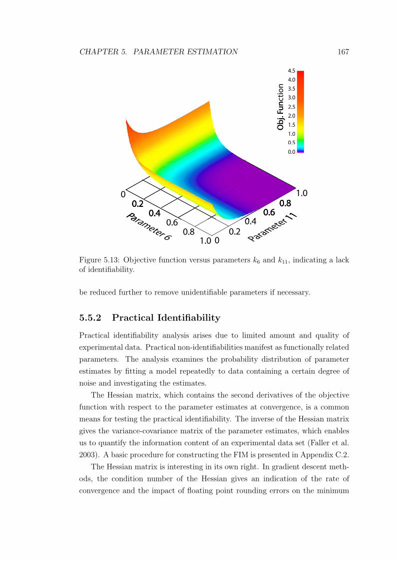
CHAPTER 7. A PROPOSED METHODOLOGICAL FRAMEWORK 221
the two enzymes
VARG =V ARG
max(1 +
KARGaODC
[ODC]
)γ1·
[Arg]
KARGmArg
1 +[Arg]
KARGmArg
(7.6)
where KARGaODC (μM) represents the activation coefficient of the ODC concen-
tration ([ODC]) on the enzyme activities of arginase; and γ1 stands for the
activation strength. These two parameters are assumed to vary between 0 and
10.
We performed an optimization-based simulation study on the arginine metabolism
module to examine the presence of this regulatory relationship in T. brucei. The
rate equations of the constituent enzymes, including arginine uptake, ODC and
arginase, are expressed in Equation (4.23) and Equation (4.2) (in Chapter 4) and
Equation (7.6), respectively. The simulation results for intracellular arginine and
ornithine are shown in Figure 7.8. Both metabolites show a satisfactory match
with the experimental data, where arginine dynamics observed in the procyclic-
form T. brucei are assumed as the true experimental data.
0 500 1000 1500 2000 2500 3000Time (min)
0
500
1000
1500
2000
2500
3000
Arg
Con
c. (μ
M)
Simulation DataObserved Values
(a) arginine
0 500 1000 1500 2000 2500 3000Time (min)
0
200
400
600
800
1000
Orn
Con
c. (μ
M)
Simulation DataObserved Values
(b) ornithine
Figure 7.8: Simulation profiles compared to experimental data for the argi-nine and ornithine dynamics computed with the modified rate of change of theenzyme arginase. In this case, arginine dynamics observed in procyclic-form T.brucei is assumed as the true experimental data. Error bars are presented whereappropriate data was available in the original papers.
However, a different mathematical model structure of the module is required
in order to interpret the dynamics properly when constant arginine concentra-
tions are assumed in the DFMO-induced experiment. Our modelling experience

CHAPTER 7. A PROPOSED METHODOLOGICAL FRAMEWORK 222
suggests that a refined rate equation of the upstream reaction of endogenous
arginine production – exogenous arginine uptake, has to be applied by incorpo-
rating the activatory regulation from the enzyme ODC as follows
VArgPt =V ArgPt
max(1 +
KArgPtaODC
[ODC]
)γ2·
[Arg]exg
KArgPtm
1 +[Arg]exg
KArgPtm
(7.7)
where KArgPtaODC (μM) represents the activation coefficient of the ODC concentra-
tion ([ODC]) on the enzyme activities of arginine transporter; and γ2 stands for
the activation strength. The two parameters are assumed to vary between 0 and
10.
We performed another simulation study on the arginine metabolism module,
where the rate equations of ODC, arginine uptake and arginase are expressed in
Equation (4.2) (in Chapter 4), Equation (7.7) and Equation (7.6), respectively.
The simulation results of the intracellular arginine and ornithine are shown in
Figure 7.9. Both metabolites can be correctly estimated in terms of both the
transient changes and exact values of the intracellular concentrations.
0 500 1000 1500 2000 2500 3000Time (min)
0
200
400
600
800
Arg
Con
c. (μ
M)
Simulation DataObserved Values
(a) arginine
0 500 1000 1500 2000 2500 3000Time (min)
0
200
400
600
800
1000
Orn
Con
c. (μ
M)
Simulation DataObserved Values
(b) ornithine
Figure 7.9: Simulation profiles compared to experimental data for the arginineand ornithine dynamics computed with the modified rate of change of the enzymearginase and arginine transporter. In this case, constant arginine concentrationsare assumed as the true experimental data. Error bars are presented whereappropriate data was available in the original papers.
Applying the fitted module of arginine metabolism, we determined that the
quantitative behaviour of the module is not compatible with both experimental
data sets. By in silico investigation, we identified a regulatory link between the

CHAPTER 7. A PROPOSED METHODOLOGICAL FRAMEWORK 223
arginine uptake, arginase and ODC enzymes as an essential feature of arginine
metabolism. Biological experiments are necessary to experimentally verify this
prediction in T. brucei, however. A recent biological experiment performed
by Darlyuk et al. (Darlyuk et al. 2009) observed that in L. donovani exogenous
arginine uptake increased significantly during cell starvation and was suppressed
to avoid intracellular arginine accumulation (which is toxic to the cell growth)
when polyamines are abundant or genetically ablated from the parasite, which
supports the existence of this link in T. brucei.
7.7 Model Reconstruction
Briefly, our proposed approach attempts to identify the ill-defined reaction(s)
by reducing the whole system into sub-systems for the examination of structure
correctness via global optimization. In Model Structure Exploration phase, we
discovered a potential regulatory link between arginase, arginine transporter
and ODC, which is postulated to be of biological importance in the regulation
of intracellular polyamines contents.
According to the decompositional rules, there are two situations where the
phase of model decomposition terminates and the phase of model reconstruction
begins. The first is, when in a certain stage of model decomposition, the module
becomes ‘elementary’ and has deficiencies in the mathematical model structure.
‘Elementary’ refers to the situation where further decomposition of the module is
not possible. The second is when the resulting module can produce a satisfactory
match with experimental data for the components of interest.
The former restricts a detailed examination of the model structure correct-
ness to a local area of the module. The phase of Model Structure Exploration
is activated in this situation for scrutinizing only the reactions included in the
resulting module for appropriate kinetic characters. The latter situation implies
that the reactions removed from the previous stages of the decomposition pro-
cedure may be incorrectly described, and the kinetic mechanisms related should
be examined for appropriate variants.
To continue the investigation of model structure deficiency, Model Recon-
struction has to be performed in order to scrutinize the reactions in the rest of
the mathematical model. This suggests a procedure where reactions that com-
prise the initial model but are excluded from the structurally-correct module
are added back to the module following the same rules for deciding the bound-

CHAPTER 7. A PROPOSED METHODOLOGICAL FRAMEWORK 224
ary components defined in the proposed decompositional approach. Thereby,
model reconstruction, which is an iterative procedure, can be understood as the
reverse of model decomposition. In this phase of the methodological framework,
we intend to explore the ill-defined kinetic characters of the modules devel-
oped in each stage of the decomposition procedure via global optimization. The
proposed mathematical model structure for arginine metabolism (discussed in
Section 7.6.1) is applied throughout the in silico investigation.
Certainly, designing sound mechanisms to describe enzyme kinetics depends
on how much biological knowledge is available for the reaction(s) in question.
When lacking biological evidence, it is an intrinsic impossibility for ambiguously-
defined reactions to be thoroughly studied. Therefore, the level to which the
process of model decomposition or reconstruction is applied is in most cases
determined by the richness of available biological information.
7.7.1 Experimental Results
We perform optimization-based simulation of the modules developed in all three
stages of model decomposition. To maintain consistency in the use of experi-
mental data, arginine dynamics assumed by Fairlamb et al. for the bloodstream-
form T. brucei in response to DFMO inhibition are applied. Accordingly, Equa-
tion (4.2) (in Chapter 4), Equation (7.7) and Equation (7.6) proposed in Sec-
tion 7.6.1 are employed to model the reactions relevant to arginine metabolism.
Satisfactory simulation results were obtained for the fitted polyamine biosyn-
thetic module in Figure 7.3(C), hence supporting our mathematical formulation
of the reactions in the considered sub-system.
A satisfactory match with the experimental data was also obtained for the
module in Figure 7.3(B), where GSH and GspdSH were boundary components.
Solving the model of the trypanothione biosynthetic module shown in module in
Figure 7.3(A) however resulted in simulation results not consistent to experimen-
tal data, particularly for the metabolites glutathione and GspdSH. In addition
to the introduction of reactions associated with trypanothione synthesis, the
major difference between the modules lies in the inclusion of the glutathione
biosynthetic sub-pathway, where, for the former, glutathione is solved over time
simultaneously with other variable components.
In the following section, we focus on evaluating the correctness of the math-
ematical equations that are currently applied to describe the kinetics of the

CHAPTER 7. A PROPOSED METHODOLOGICAL FRAMEWORK 225
bi-functional enzyme trypanothione synthetase, which catalyzes the reactions
associated with trypanothione synthesis (defined in Equations (4.27) to (4.30)
in Chapter 4). Optimization-based simulation is performed on the entire model,
where glutathione is defined as a known input, approximated with the experi-
mentally measured dynamics.
Investigation on the kinetic character of trypanothione synthetase and
amidase with DFMO-induced experimental data
Our literature research reveals two different GSH dynamics under the DFMO
treatment. Specifically, GSH concentrations were observed to increase by almost
80% (Fairlamb et al. 1987) or reduce by 60% (Xiao et al. 2009) of the controlled
level. The dynamics of other metabolites including spermidine, GspdSH and
trypanothione did not differ significantly between the two experimental settings.
The simulation results for putrescine, spermidine, GspdSH and trypanothione
compared to the observed values from Fairlamb et al. are shown in Figure 7.10,
where the glutathione dynamics are approximated using a 3rd-order polyno-
mial function (fitted to the observations by Fairlamb et al.) and a first-order
exponential function (fitted to the observations by Xiao et al.).
Figure 7.10 indicates that trajectories of the fitted model with different input
functions for glutathione can closely reproduce the experimental data in a self-
consistent manner. Model predictions for putrescine dynamics (Figure 7.10(a))
with two different inputs are almost identical in terms of both the trend and the
estimated values of the concentration changes. Model predictions for the dynam-
ics of spermidine (Figure 7.10(b)), GspdSH (Figure 7.10(c)) and trypanothione
(Figure 7.10(d)) share certain similarities in the transient changes in concentra-
tion, even though they differ in exact values with respect to experimental data.
Interestingly, concentration levels of spermidine and trypanothione are raised
(with both inputs) by about 12% and 40%, respectively, of the initial values
within 6 hours of drug addition, followed by a gradual decrease later on.
One explanation for our in silico observations that spermidine and trypan-
othione concentrations increase sharply is that T. brucei may attempt to restore
proliferation in the early stage of trypanosomal infection via defense mecha-
nisms, for example, the well-known antioxidant enzyme defense system based on
trypanothione (Schirmer et al. 1987). Recently, the compensatory mechanism
of arginase up-regulation by activated macrophages has been observed in Leish-
maina (Kropf et al. 2005) and T. cruzi (Peluffo et al. 2004) to counteract parasite

CHAPTER 7. A PROPOSED METHODOLOGICAL FRAMEWORK 226
0 500 1000 1500 2000 2500 3000Time (min)
0
100
200
300
400
500
600
Put C
onc.
(μ
M)
Simulation Data 1Simulation Data 2Observed Values
(a) putrescine
0 500 1000 1500 2000 2500 3000Time (min)
0
500
1000
1500
2000
2500
3000
Spd
Con
c. (μ
M)
Simulation Data 1Simulation Data 2Observed Values
(b) spermidine
0 500 1000 1500 2000 2500 3000Time (min)
10
20
30
40
50
Gsp
dSH
Con
c. (μ
M)
Simulation Data 1Simulation Data 2Observed Values
(c) GspdSH
0 500 1000 1500 2000 2500 3000Time (min)
100
200
300
400
500
600
TSH
Con
c. (μ
M)
Simulation Data 1Simulation Data 2Observed Values
(d) trypanothione
Figure 7.10: Simulation profiles compared to observed values (Fairlamb et al.)for the key metabolites when glutathione dynamics is approximated using differ-ent experimental data reported by Fairlamb et al. (continuous line) and Xiao etal. (dotted line). Error bars are presented where appropriate data was availablein the original papers.
infection; however this mechanism has not been verified to exist in T. brucei.
Further work is required in order to gain new insights on defense mechanisms in
trypanosomes, and consequently to unravel the underlying causes.
A mathematical model is valid only if it can reproduce all existing data
consistently, given that the data is relatively accurate and the sets are compatible
with each other. To illustrate this principle, we continue the evaluation of the
mathematical equations with another set of experimental data that is suitable
for this investigation, namely the gene-knockdown profile of spermidine synthase
measured by Xiao et al. (Appendix A.2). Since the dynamic behaviour of
ornithine was not reported, intracellular putrescine combined with dAdoMet and
glutathione are taken as the model inputs. All three inputs are approximated
using 3rd-order polynomials.

CHAPTER 7. A PROPOSED METHODOLOGICAL FRAMEWORK 227
In the RNAi knockdown experiment, spermidine synthase mRNA and protein
were reduced up to 90% of the original value by day 2 after the RNAi induction.
No correlated changes in the expression levels of other polyamine biosynthetic
enzymes, trypanothione synthetase or trypanothione reductase were observed in
the in vivo experiment. In accordance with biological information, the inhibition
of enzyme SpdS is assumed to follow a time-dependent exponential decay that
replaces the parameter V SpdSmax in Equation 4.16, expressed as
V SpdSmaxSS · e−λ·t (7.8)
where V SpdSmaxSS stands for the maximum velocity of spermidine synthase under
normal conditions. Parameter λ is solved by simple curve fitting using the
qualitative description of the enzyme dynamics with addition of DFMO and
takes a value of 0.0015 in this instance. The time span from 0 to 6 days is
covered by the experiment.
The resulting time courses of the module for intracellular spermidine and
GspdSH are shown in Figure 7.11. Both metabolites return a satisfactory match
with the experimental data in terms of the transient changes in concentration,
though it is not perfect with regard to the estimated concentration levels. Model
prediction of the trypanothione dynamics reveals rather interesting behaviour, as
shown in Figure 7.12. A high peak within the first 2 hours of DFMO treatment
is observed and presented in more detail in the enlarged inset to discern the peak
clearly.
Overall, in the phase of model reconstruction, the mathematical model struc-
ture of the polyamine biosynthetic module was evaluated to be correct in terms
of the DFMO inhibition data. The entire model of trypanothione metabolism
with glutathione as a known input can reproduce both experimental data sets in
a consistent manner. However, it is not possible to assert that the mathematical
equations currently in use to model the bi-functional enzyme trypanothione syn-
thetase and the trypanothione redox system are definitely correct; the structure
may be disproved later when more experimental observations about the system
are available.
Prior to the step of Model Structure Exploration, which searches for model
variants of the remaining sub-systems, targeted in vivo experiments are required
to distinguish between the two conflicting observations on glutathione dynamics
in response to DFMO inhibition and to explain the abrupt elevation of the

CHAPTER 7. A PROPOSED METHODOLOGICAL FRAMEWORK 228
0 2000 4000 6000 8000Time (min)
0
500
1000
1500
2000
Spd
Con
c. (μ
M)
Simulation DataObserved Values
(a) spermidine
0 2000 4000 6000 8000Time (min)
0.001
0.01
0.1
1
10
100
1000
log
Gsp
dSH
Con
c. (μ
M)
Simulation DataObserved Values
(b) GspdSH
Figure 7.11: Simulation profiles of spermidine and GspdSH compared to geneknockdown data by Xiao et al.. In the simulation plot of GspdSH, the data pointmeasured after four days of RNAi knockdown of spermidine synthase seems tobe corrupted with large noise level. Error bars are presented where appropriatedata was available in the original papers.
metabolite concentration levels within the first 6 hours of DFMO treatment.
Additionally, biological information about other organisms may suggest changes
that can be used to further refine the model of T. brucei. As stated in Chapter 4
(Section 4.3.3), glutathione was found to enable a 15-fold activation of GspdSH
hydrolysis (Fyfe et al. 2008) in Escherichia coli. This promotes an investigation
on the potential stimulating effect that GspdSH exercises on amidase activity in
T. brucei, which may give rise to a modification of the mathematical expression
of the kinetic character of the enzyme.
The remarkable improvement obtained for the fitted model of trypanothione
biosynthesis when glutathione dynamics are given as an input implies that the
glutathione biosynthetic sub-pathway may be ill-characterized. This may be
ascribed to the kinetic mechanisms of reactions related to glutathione production
wrongly formulated or to some elementary reactions vital for the regulation of
glutathione metabolism being missing from the current topological structure. We
have explained that the kinetic character of the upstream reactions of glutathione
production cannot be investigated by our approach, because dynamic responses
of the intermediate metabolites of this sub-pathway (cysteine and gGluCys)
in response to DFMO inhibition have never been measured in vivo, thus the
optimization-based decompositional approach cannot be applied.
A recent hypothesis that the γ-glutamyl transpeptidase cycle is present in T.
brucei (Mike Barrett, personal communication, March 2009) provides support

CHAPTER 7. A PROPOSED METHODOLOGICAL FRAMEWORK 229
0 2000 4000 6000 8000Time (min)
0.01
0.1
1
10
100
log
TSH
Con
c. (μ
M)
Simulation DataObserved Values
0 60 1201
10
100
Figure 7.12: Simulation profiles of trypanothione compared to gene knockdowndata from Xiao et al.. Inset in the figure refers to the enlarge version of theindicated dynamics of trypanothione over the first two hours of DFMO addition.Error bars are presented where appropriate data was available in the originalpapers.
for our postulation of the incompleteness of the network topology concerning glu-
tathione biosynthesis. The γ-glutamyl transpeptidase cycle may have an impor-
tant role in regulating glutathione dynamics, which accounts degradation of glu-
tathione into cysteine, glycine and glutamate via intermediate compounds cys-
teinylglycine and (5-L-glutamyl)-L-amino acid, and regeneration of glutathione
from the products. The γ-glutamyl transpeptidase cycle is supplementary to
research in the area of glutathione metabolism and function (Vina et al. 1989).
This concept is worth consideration for improved comprehension of glutathione
metabolism in T. brucei when relevant biological evidence is substantial enough
for the investigation. Model structure correctness of the glutathione-centered re-
actions can only be assessed when the glutathione dynamics are modelled. This
involves incorporating the glutathione biosynthetic sub-pathway, the γ-glutamyl
transpeptidase cycle and the GspdSH activatory function into a unified environ-
ment.

CHAPTER 7. A PROPOSED METHODOLOGICAL FRAMEWORK 230
7.8 Remarks on Modelling Framework
In summary, we have demonstrated that the proposed methodological frame-
work can be applied to systematically guide and refine the model construction
procedure of biological systems when prior knowledge about the system is in-
complete and the available experimental data is sparse. We illustrate that by
means of optimization-based simulation, biological hypotheses describing differ-
ent underlying processes can be formulated mathematically and evaluated by
comparison to experimental data.
Defining a set of candidate models for complex biological systems is an impor-
tant part of model development, but often underemphasized due to the amount
of work required and the lack of established methods. Only a few studies have
examined the impact of model structure on interpreting biological processes.
The discrepancy between model predictions and experimental data emphasizes
the necessity of investigating various structures for the mathematical models.
Swameye et al. (Swameye et al. 2003) compared models of the JAK-STAT
signalling pathway with the assumption of a feed-forward cascade versus a model
capturing the cycling capacity of STAT5 and identified that the cycling path is
an essential feature of the JAK-STAT core module. The authors underlined
the essentiality of detailed knowledge of biological pathways for establishing
mechanistic models. Takors et al. (Takors et al. 1997) performed a simulation-
based study to discriminate between 10 competing macrokinetic models, where
the best suitable model was selected according to the discrimination criteria
based on probability theory rather than the traditional sum of squares. The
authors also highlighted the importance of the identification and discrimination
of macrokinetic models in bioprocess development.
The works by the authors above have two features in common. First, model
discrimination is largely reliant on experimental data for comparison, and sec-
ond, the assumptions about possible system structures for constructing com-
peting models were taken directly from biological observations measured under
different conditions. By contrast, in our study, no biological information about
the trypanothione metabolic system is available to aid the definition of candi-
date models. It is not surprising that for such a complex and poorly understood
system, relying on repetitive in vivo experiments to discover unknown regula-
tory mechanisms or to clarify ambiguous concepts about the system would be
impractical.

CHAPTER 7. A PROPOSED METHODOLOGICAL FRAMEWORK 231
We made great efforts by means of optimization-based simulation to investi-
gate physical grounds of the underlying biological processes. We proposed two
kinetic mechanisms for arginine metabolism from the two contradictory sets of
experimental data. Both proposed mechanisms imply a potential regulatory link
between the enzymes of polyamine biosynthetic sub-pathway. We also identified
the parts of the model for which structure exploration via computational simu-
lation is not allowed due to the absence of sufficient biological observations. Our
in silico investigations provide advice for biologists on design of in vivo experi-
ments and analysis of the experimental results in order to enable the exploration
of model structure, to discriminate between rival hypotheses and to gain new
insights about the system.
Recently, a Bayesian approach has been applied to model selection of bio-
logical networks (Vyshemirsky 2007), which uses the rules of probability theory
to select among different models. The probability-based approach for model
discrimination was first proposed by Box and Hill (Box and Hill 1967) based
on the concept of entropy. The mathematical method developed by Box and
Hill can also be applied to guide the design of ‘new’ experiments so as to attain
maximum expected discrimination among rival models that would fit the data
equally well. The authors used the method to identify the operating point (e.g.
time, temperature, etc.), at which rival models can be discriminated.
As stated by Box and Hill (Box and Hill 1967), experiments in any given
situation can only be conducted within the physical constraints of the experi-
mental setup, e.g. the time span or operating temperature. This is the so-called
operability region. In the context of biological experiments, the operability re-
gion frequently corresponds to the time span, which can be very extensive, and
it may be impossible to cover the full range. In terms of an experimental design
for model discrimination, our in silico investigations can help improve the effi-
ciency of ‘new’ biological experiments by advising experimentalists to focus on
the operability region where the discriminatory power of the experiments can
be increased. Time-series concentration profiles estimated via computational
simulation, for instance the results in Figure 7.10 and Figure 7.12, indicate that
an enhanced discriminatory capability can be obtained by measuring the system
behaviour over the first 6 hours after DFMO addition.
It is worth emphasizing that a mathematical model is only an approxi-
mate representation of the phenomena being studied; it is useful for achieving
a system-level understanding with the assistance of computational simulation.

CHAPTER 7. A PROPOSED METHODOLOGICAL FRAMEWORK 232
However, in reality, no biological systems will follow a mathematical model ex-
actly. When the number or the precision of observed data points increases, it is
likely that revision of the model will be necessary.
During the course of system identification, it is always important to be re-
minded of the saying from Box (Box 1979) that “all models are wrong, only some
are useful”. Models should be designed and evaluated with respect to their in-
tended use. Asking whether a model is correct or wrong is not appropriate.
Rather, one should ask if the model is valid in representing the essential features
of the system and if uncertainty in the model will result in noticeable effects on
model inferences, and consequently, the confidence in model applicability.
Our study is intended to, given certain experimental data, seek for kinetic
mechanisms of the reactions that can produce a reasonably good description
of the underlying biological properties. The adequacy of model structures in
predicting the system dynamics in different experimental conditions can only
be determined when relevant biological evidence is available for the system.
We argue that model structure is correct if it can reproduce the existing data
consistently within the limit of the modelled biology, whereby models can be
assumed as a good representation of reality.
Remarks on Model Decomposition
We noticed that our proposal on model decomposition and the approach pro-
posed by Koh et al. (Koh et al. 2006) appears similar to a certain degree, for
instance, modules are defined as closed systems. However, fundamentally, they
are distinct approaches as summarized below:
1. In Koh et al.’s approach, model decomposition intends to solve the problem
of parameter estimation, assuming the structure as correct. In contrast,
in our approach, model decomposition intends to solve the problem of
structure identification, where ill-defined reactions can be identified via a
qualitative comparison between model simulation results and experimental
data.
2. In Koh et al.’s approach, a typical evolutionary procedure is applied to
the parameter estimation procedure, which is inactive until all the model
components (so-called sub-systems in our approach) are derived. Their
approach chooses a particular component for parameter estimation that
contains the ‘richest’ information on kinetic parameters and experimental

CHAPTER 7. A PROPOSED METHODOLOGICAL FRAMEWORK 233
data, which enables the remaining components to be solved in sequence. In
our approach, an optimization-based simulation is performed once a sub-
system is derived and the quality of fit and the availability of experimental
data determines if further levels of model decomposition are required.
3. In Koh et al.’s approach, model decomposition begins with a single state
variable and components are derived by adding reactions and metabolites
associated with the state variable according to predefined criteria. In our
approach, model decomposition begins with an entire model and at each
stage, ‘unmeasured metabolites’1 and associated reactions are removed in
a recursive manner until ‘known metabolites’ are obtained which can be
used as module boundaries. It is not clear how Koh et al. initiated the
decompositional procedure, particularly, the selection of the first state vari-
able. Our approach takes advantage of the relationship between structural
topology and functional modules discovered via structural modelling to
initialize the decompositional procedure.
4. In Koh et al.’s approach, model components share inputs or outputs, how-
ever in our approach sub-systems may be subsets of other sub-systems.
The modularity of the trypanothione metabolic pathway (shown in Fig-
ure 4.1) was also explored using a topology-based decomposition strategy. In
order to detect sub-networks, MatlabBGL package2 was used to determine a
betweenness measure based on the shortest path (see Section 2.5 in Chapter 2).
An adjacency matrix was formulated as an input to the algorithm, with each
path (reaction) given equal weight for the pathway vertices (metabolites). An
adjacency matrix (A) of a directed graph (such as the trypanothione pathway)
represents which vertices are adjacent to which other vertices; the entry A(i, j)
is equal to 1 if there is an edge from vertex i to vertex j, otherwise it is 0.
The highest edge betweenness values were obtained for the paths between the
following pairs of metabolites: spermidine, glutathione and trypanothione, and
trypanothione and TS2. These two paths divide the pathway into two topo-
logically isolated sub-networks, which corresponds to the functionally isolated
sub-networks identified in Chapter 3. This observation supports our decom-
position approach, where trypanothoine, which is the joint between the two
1in our context, unknown metabolites refer to metabolites for which no experimental datais available.
2http://www.stanford.edu/∼dgleich/programs/matlab bgl/

CHAPTER 7. A PROPOSED METHODOLOGICAL FRAMEWORK 234
sub-networks, is selected as the initial point. In this way, each sub-network
can be explored independently, which is complemented by an investigation of
interactions among the modules.
Remarks on Model Structure Exploration
The phase of Model Structure Exploration in our proposed framework shares
some similarities with the concept of Model Selection. Model Selection refers
to the process of selecting the ‘best’ model from a given set of potential models
(Anderson et al. 2000). A typical selection strategy is, starting from the smallest
model or from the full model, to add or delete one parameter until a predefined
critical significance is reached. The present study of structure exploration differs
from the framework of model selection in several aspects, including
• First, how a set of candidate models was defined. In the current study,
candidate models were designed by revising the kinetic characters of reac-
tions of the intact model, which is guided by available information from
the literature. When a candidate model is proposed, a global optimiza-
tion task is applied to examine the model correctness in terms of whether
the simulation results can reproduce the observed experimental data. The
number of optimization tasks to be performed is equal to the number of
candidate models proposed, the network topology of which remains fixed
for individual tasks. This is in contrast to the (automatic) procedure of
model selection, which is often realized via a single optimization task that
consists of a number of runs. At each run, the network topology examined
is distinct in terms of which parameters are contained.
• Second, how the ‘best’ candidate is selected. In our study of structure
exploration, a qualitative comparison method is applied, which indicates
that the model with simulation curves most similar to the experimental
data is retained as a good candidate. On the contrary, a pre-specified
criteria is often set in the model selection procedure for a quantitative
comparison of model variants, and the one with the smallest fitness value
is chosen as the ‘best’ model.
Both Model Selection and Structure Exploration procedures are computa-
tionally expensive, particularly for applications when, for Model Selection, no
prior knowledge is given, regarding the sequence or combinatory form in which

CHAPTER 7. A PROPOSED METHODOLOGICAL FRAMEWORK 235
the parameters should be considered and, for Structure Exploration, regarding
the types of kinetic characters to be introduced and on which enzymatic reac-
tions they should be investigated. The automatic procedure of model selection
is more likely to lead to models without biological interpretation, thus models
without biological support should be excluded from the set of candidate models.
In summary, through the processes of model decomposition, model structure
exploration and model reconstruction, a sub-system of the initial mathematical
model (polyamine metabolism) was evaluated and refined to a structurally cor-
rect variant. The polyamine biosynthetic sub-pathway will now be considered
in the phase of model validation.
7.9 Model Validation of Polyamine Metabolism
Model validation is concerned with proving that the model is an adequate repre-
sentation of reality (Neelamkavil 1987). The substantial value of mathematical
models lies in their power to predict system behaviour characterized by new
and fresh data. As previously stated, there is no ultimate proof of correctness
of a mathematical mechanistic model; knowledge about physical insights of the
underlying processes will always increase as more biological evidence becomes
available. In this section, we aim at investigating the general applicability of
the model of the polyamine biosynthetic sub-pathway. Model validation may
challenge the model credibility and encourage further model refinement.
Comparisons of in silico predictions with experimental data enable the eval-
uation of model credibility in interpretation and prediction of biological phe-
nomena. Discrepancy in the comparisons can be used to systematically identify
potential improvements to the model and suggest specific experiments to verify
hypothesized model modifications.
For example, Garfinkel (Garfinkel 1971) suggested computer simulation of
liver gluconeogenesis as a resolution to elucidate the contradictory results (lower
malate concentration vs. higher malate concentration) observed by two groups
of investigators. A critical computer experiment performed in the work is the
simulation of the second data set using the model developed for the first data
set, which revealed the parameters that caused the apparent discrepancy between
the findings. This in silico experiment shows that the same model with different
parameter values can produce behaviour qualitatively consistent with individual
data sets.

CHAPTER 7. A PROPOSED METHODOLOGICAL FRAMEWORK 236
Model applicability of the polyamine biosynthetic sub-pathway is assessed
by comparison between the model predictions and an independent data set ob-
tained in a distinct dynamic state of the system. The experimental data from
DFMO induction and gene knockdown were collected where the system was
initiated with different conditions3. We use physiological steady-state concen-
trations and DFMO-induced data as inputs to the model validation procedure,
tackled by the multi-objective optimization algorithm, MoPSwarm, proposed in
Chapter 6. Gene-perturbed data (so-called validation data) is used to assess
the model applicability with the parameter estimates in response to different
chemical interventions.
7.9.1 Objective Function
Parameter values are refined by comparing simulation results with experimental
measurements. A modified G-test was used as the objective function to measure
the goodness of fit of the model defined in both conditions – polyamine steady-
state model and polyamine perturbed model. The general formula for the test
statistic G is
G = 2 ·∑
i
Oi · ln(Oi
Ei
)
In our study, the term Oi multiplying the natural logarithm in the formula was
removed in order to prevent metabolites with large concentrations dominating
the objective function value. This leads to the following expression
G(p, t) =∑
t
ln(O(t)
E(p, t)) (7.9)
where ln denotes the natural logarithm and the sum is taken over all sampling
points. In the context of optimization of biological pathways, there are discrete
time points. Here, p is the decision vector to be tuned. O(t) and E(p, t) are the
observed data and model simulation, respectively, given at time point t.
As illustrated in Figure 5.3 in Chapter 5, objective functions based on resid-
ual errors are insufficient for parameter estimation problems when the optimiza-
tion performance is measured by more than one criteria. This is the case for
3Large differences in initial conditions of model simulation and experimental settings causedifficulty in presenting data in the same figure without losing the dynamic trends. A loga-rithmic axis is used for some metabolites whose initial conditions differ considerably in thesimulations and experimental observations.
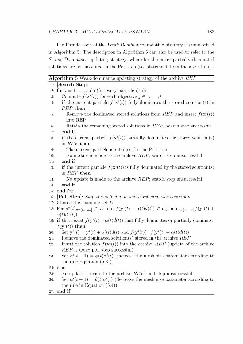
CHAPTER 7. A PROPOSED METHODOLOGICAL FRAMEWORK 237
polyamine steady-state model, where the concentrations of model variables are
constrained by two criteria, namely (1) the residual of observed data and sim-
ulation results and (2) the trend of change of concentrations. A feasible set of
solutions should be tuned for the acquisition of both criteria. We propose the
use of a dynamic penalty function to tackle the second criterion – the trend of
change of concentrations.
A general form of distance based penalty method incorporating a dynamic
aspect based on length of search, l, is as follows, according to the description
given by Smith and Coit (Smith and Coit 1997)
fp(x, l) = f(x) +∑i=1
Si(l)dki
where Si(l) is a function monotonically non-decreasing in value with l. di is the
distance matric of constraint i (e.g. number of generations or the number of
solutions searched) applied to solution x and k is a user-defined exponent, with
values of k of 1 or 2 often used.
The penalty function proposed in this study is defined as follow:
P (p) =m∑
n=1
n · ln(
1+ | E(p, n) − E(p, n + 1)
E(p, n)|)
(7.10)
where ln(1+ | · |) is designed to accurately compute (small) absolute values in | · |that quantify the change in concentration of simulation results calculated at the
boundaries of the time interval. n is the index of the time interval for n = 1 to
m intervals in a time span divided into discrete time points. n is monotonically
non-decreasing, acting as Si(l) in the general expression.
The idea of introducing the penalty function is to incorporate a dynamic as-
pect, which increases the severity of the penalty as the integration or simulation
progresses. The objective function for the polyamine steady-state model with
both criteria is then formulated as below (for a minimization problem):
Gp(p, t) = G(p, t) + P (p) (7.11)
where G(p, t) is the unpenalized objective function and P (p) is the penalty
function.
In practice, penalty functions typically require problem specific tuning to
perform well. A major difficulty of combining all objectives into a single objective
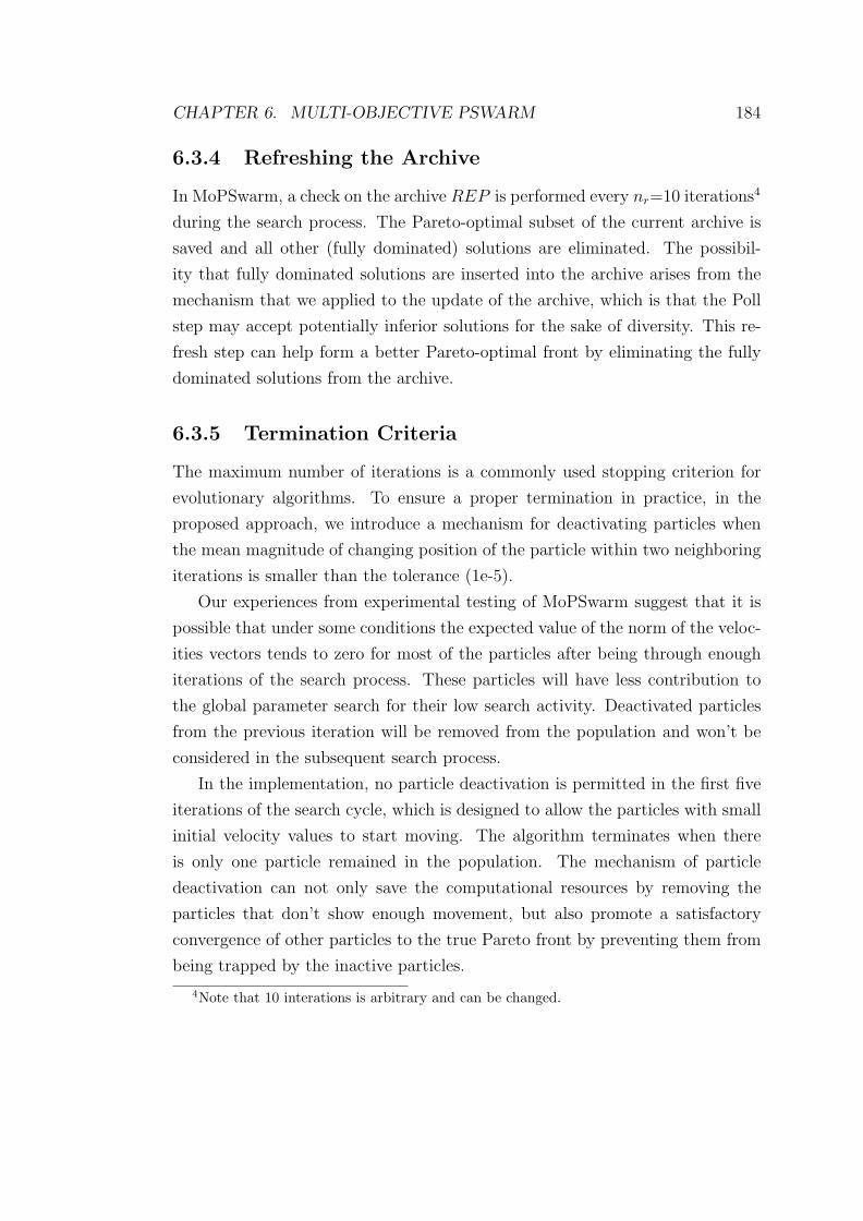
CHAPTER 7. A PROPOSED METHODOLOGICAL FRAMEWORK 238
lies in determining a multi-criteria fitness value to summarize the degree of
satisfaction of all the individual objective. We investigated the appropriateness
of several definitions of the penalty function P (p) differing in the explicit form
of Si(l). The penalty function defined in Equation (7.10) was found to be the
most suitable expression for the problem of interest.
7.9.2 Hill Equation Approximation to Spermidine
In order to evaluate the model predicability, and thus assess its applicability,
interaction of the polyamine biosynthetic module with the rest of the trypan-
othione metabolic system has to be modelled explicitly (polyamine biosynthetic
module is represented as a closed system in the previous phases), which in-
cludes spermidine consumption in GspdSH production and its regeneration from
GspdSH hydrolysis. However, as indicated in the study carried out in the phase
of model reconstruction, the correctness of the current mathematical equations
used to model the bi-functional enzyme trypanothione synthetase is uncertain.
To render predictive power to this module, a black-box structure has to be ap-
plied to the module output – spermidine, to approximate its participation in
other biochemical reactions.
Selecting an appropriate black-box structure to describe non-linear dynamics
is a difficult problem. As introduced in Chapter 2, model structures can take
the form of power series polynomial, fuzzy logic or neural network. We employ
the Hill equation in the form of a regressive function to approximate spermidine
participation in other metabolic functions of the system, as shown below
Vspdout = V spdoutmax ·
([Spd]
Kspdoutm
)n
1 +
([Spd]
Kspdoutm
)n (7.12)
Thereby, spermidine dynamics is modelled by the following differential equation
d[Spd]
dt= VSpdS − Vspdout
where the rate equation of enzyme VSpdS responsible for spermidine production
is given in Equation (4.16) in Chapter 4.
An advantage of using the Hill equation (Equation (7.12)) to approximate the
non-linear dynamics of spermidine participation is that the parameters involved

CHAPTER 7. A PROPOSED METHODOLOGICAL FRAMEWORK 239
Time-dependent Differential EquationsVariables
[Met] d[Met]dt
= VMetPt − VMAT + VMetRcy
[AdoMet] d[AdoMet]dt
= VMAT − VAdoMetDCT − VAdoHcy
[dAdoMet] d[dAdoMet]dt
= VAdoMetDCT − VSpdS
[Arg] d[Arg]dt
= VArgPt − VARG
[Orn] d[Orn]dt
= VARG − VODC
[Put] d[Put]dt
= VODC − VSpdS
[MTA] d[MTA]dt
= VSpdS − VMetRcy
[Spd] d[Spd]dt
= VSpdS − Vspdout
Table 7.1: Differential equations for the different metabolites included in thepolyamine biosynthetic sub-pathway.
in the structure have direct biological meaning: V spdoutmax – maximum velocity of
spermidine participation, Kspdoutm – half-saturation constant, and n – hill coeffi-
cient. This avoids the problem of a lack of physical insight in most cases when
black-box structures are used.
The structure of the reaction diagram of polyamine metabolism in T. brucei
is shown in Figure 7.13. The difference between this diagram and Figure 7.3(C)
lies in the aspect that intracellular spermidine is modelled as a time-dependent
variable rather than a given output approximated with measured dynamics.
Table 7.1 gives the differential equations for the different metabolites in the
polyamine biosynthetic sub-pathway.
We first carry out an optimization-based simulation of the polyamine biosyn-
thetic sub-pathway to examine if the black-box structure in the form of a Hill
equation is sufficient to reproduce observed behaviour of intracellular spermi-
dine. The simulation results of spermidine dynamics (see Figure 7.14) show a
good match with the experimental data, supporting the proposed model struc-
ture.

CHAPTER 7. A PROPOSED METHODOLOGICAL FRAMEWORK 240
Figure 7.13: The schematic representation of polyamine biosynthetic sub-pathway. Metabolites in pink, brown and green ovals represent model compo-nents that are exogenous, constant and variable, respectively. Edges representchemical conversions between model components with arrows indicating reac-tion directionality. Enzymes included in this sub-pathway are denoted with blueboxes. Intracellular spermidine is considered as a time-dependent variable. Thered oval – trypanothione biosynthesis stands for the rest of the trypanothionepathway. The dot-dashed edges represent the regulatory links predicted betweenenzymes of ODC, ARG and the arginine transport enzyme in Section 7.6.
7.9.3 Experimental Results
As introduced in Chapter 6, a common approach to model validation involves
a two-step procedure to determine the vector of estimated parameters that can
correctly describe a system’s response to perturbations. This involves fitting
model parameters to experimental data generated by a reference cell type (wild
type) and then testing this model on data generated by a variation (mutant).
The polyamine steady-state model contains, in total, 28 unknown parameters

CHAPTER 7. A PROPOSED METHODOLOGICAL FRAMEWORK 241
0 500 1000 1500 2000 2500 3000Time (min)
0
500
1000
1500
2000
2500
Spd
Con
c. (μ
M)
Simulation DataObserved Values
Figure 7.14: Simulation profiles for spermidine dynamics of polyamine biosyn-thetic sub-pathway compared to experimental data. Error bars are presentedwhere appropriate data was available in the original papers.
including 20 kinetic parameters and a set of 8 parameters for initial concentra-
tions of the model components. Our initial choices of the protein concentrations
for model simulation vary within ±20% of the physiological levels of polyamines
reported by Fairlamb et al. (Fairlamb et al. 1987) and experimentally measured
by the group of Mike Barrett (University of Glasgow). Following the conven-
tional approach, a set of parameters that can satisfy the steady-state constraint
of the sub-pathway was solved using the global optimizer PSwarm for the sim-
ulation study.
Two hundred runs of the steady-state optimization were executed in Matlab.
Each run starts with a different initial population of particles and is computed
over a simulated time span of 96 hrs (5760 minutes). The set of parameters that
gives the minimum of the objective function, Gp in Equation (7.11), is retained
for testing on DFMO inhibition data in the second step. To perform computa-
tional simulations of DFMO treatment, the time-independent parameter of ODC
concentration in the steady-state model is replaced with the exponential decay
function defined in Equation (7.4). Computational simulation of the perturbed
model failed to produce results consistent with the true perturbation data, even
with the ‘best’ set of parameters estimated from the steady state.

CHAPTER 7. A PROPOSED METHODOLOGICAL FRAMEWORK 242
The failure in model validation of the polyamine sub-pathway demonstrates
that the conventional approach is incapable of tackling the problem of interest,
which is characterized by complex non-linearity of kinetics and high-dimentional
parameter space. The critical challenge of relying on the parameter estimates
solved from the steady state, serving as the first step of the conventional model
validation procedure, carries with it an important message that fitting a steady
state model is a weaker criterion than that of a model of time dependent pro-
cesses describing the temporal behaviour of the model components.
We chose to apply the proposed approach – MoPSwarm – to model valida-
tion of the polyamine biosynthetic sub-pathway. Of 28 unknown parameters, 20
kinetic parameters (k1 to k20) are common to both steady-state and perturbed
model. The set of 8 parameters of initial concentrations (k21 to k28) is specific to
the steady-state model, assumed to vary within ±20% of the reported physiolog-
ical levels. In terms of the mathematical representation, ODC concentration is
a time-invariant parameter for the steady-state model and expressed as a time-
dependent exponential decay for the perturbed model. This aims to mimic the
time-dependent behaviour of DFMO transport across the cell membrane and
into the cell to react with ODC.
Trade-off solutions between the two objectives, defined by Equation (7.11)
for the steady state and Equation (7.9) for the perturbed state, are solved with
MoPSwarm and presented in Figure 7.15. The maximum number of iterations
was set to 1000 and 20 particles were used in the initial population. The search
process of the algorithm terminated at 807 iterations due to there being only a
single particle remaining. Ten optimization runs with different initial random
populations seeds were performed with MoPSwarm.
The selection of good parameter sets is conducted according to a quantitative
comparison method. This type of comparison method is based on a goodness-
of-fit criterion, which is generally applied in the optimization problems where
the emphasis is on the accuracy of the results. We employed the Root Mean
Square (also known as the quadratic mean) to rank the solutions from all ten
simulations. This measure is a common method of defining the importance of
solutions with respect to satisfying both objectives, and is given as
Rms =
√√√√( Objissmax(Objiss)
)2
+
(Objiptb
max(Objiptb)
)2
(7.13)

CHAPTER 7. A PROPOSED METHODOLOGICAL FRAMEWORK 243
0 50 100 150 200Steady-state Condition
10
15
20
25
30
35
40
Pert
urbe
d C
ondi
tion
Figure 7.15: Trade-off solutions of the polyamine model solved by MoPSwarm.The solutions show a good diversity covering a wide range of the fitness land-scape, and the corresponding Pareto front is discontinuous. The point denotedwith a filled circle is the ‘best’ solution of all ten runs as defined by Equa-tion (7.13).
where Objss and Objptb are the values of objective functions responsible for the
steady state and perturbed state given by individual solution i. Note that the
objective function values have been normalized so that they fall in the range
of 0–1, which prevents large absolute values from skewing the metric and gives
equal weighting to both objectives.
The ‘best’ solution from all ten runs, as defined by the above measure, is
selected for investigation and the Pareto front shown in Figure 7.15 corresponds
to the simulation that yielded this solution. Table 7.2 provides the predicted
values for the unknown kinetic parameters common to both objectives, obtained
from this solution (denoted with a filled circle in Figure 7.15). Rate equations
of the corresponding pathway enzymes are indicated explicitly in the table.
It is noteworthy that our model predications of the unknown parameters
are consistent with the qualitative biological information about the system,
which was detailed in Chapter 4 (Section 4.3.1). The predicated value of 778
μM for KAdoMetDCO
idAdoMet confirms the postulation by Pegg and Jacobs (Pegg and

CHAPTER 7. A PROPOSED METHODOLOGICAL FRAMEWORK 244
Jacobs 1983) that T. brucei AdoMetDC is insensitive to the reaction product
dAdoMet. A value of 2.9 μmol/min/mg for V SpdSmax indicates that the maxi-
mum velocity of T. brucei SpdS is comparable to the enzyme activity in mam-
mals as argued by Bitonti et al. (Bitonti et al. 1984) (between 0.43 and 10.95
μmol/min/mg) and disagrees with the value reported by Taylor et al. (Taylor
et al. 2008). Additionally, a large value of 40 μmol/min/mg for V MetRcymax reflects
the observation that the recycling path from MTA to methionine is an important
source of this amino acid.
Predictions on the unknown kinetic parametersEnzymes – Rate Equations Parameters Estimated ValuesODC – Equation (7.5) [ODC] 0.012 μM
AdoMetDC – Equation (7.1) & (7.2)[AdoMetDCL] 1 μM
KAdoMetDCO
idAdoMet 778 μMβ 0.94
MAT – Equation (4.14) V MATmax 1.46 μmol/min/mg
SpdS – Equation (4.16)V SpdS
max 2.9 μmol/min/mg
KSpdSiMTA 10 μM
MetRcy – Equation (4.17)V MetRcy
max 40 μmol/min/mg
KMetRcymMTA 959 μM
AHS – Equation (4.18)V AHS
max 38.9 μmol/min/mgKAHS
mAdoMet 1000 μM
ArgPt – Equation (7.7)
V ArgPtmax 0.75 μmol/min/mg
KArgPtm 1 μM
KArgPtaODC 1e-4 μM
γ2 0.21
ARG – Equation (7.6)KARG
aODC 1e-4 μMγ1 9.94
Spdout – Equation (7.12)V spdout
max 3.73 μmol/min/mgKspdout
m 1000 μMn 3
Table 7.2: Estimated values of unknown parameters of the polyamine biosyn-thetic sub-pathway.
Computational simulation of the model described in Table 7.1 using the pa-
rameter estimates in Table 7.2 thus yielded the steady state shown in Figure 7.16.
The model achieved steady state in less than two days and maintained it until
day 6 (8760 minutes). The initial condition of the steady-state model predicted
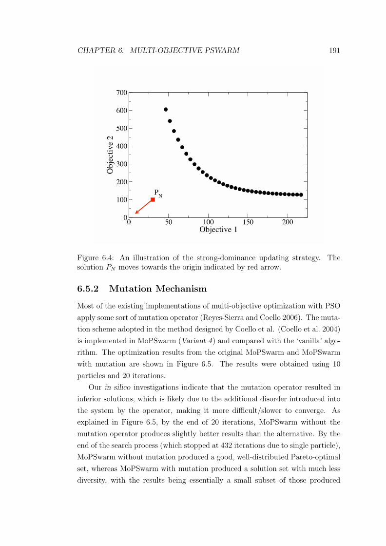
CHAPTER 7. A PROPOSED METHODOLOGICAL FRAMEWORK 245
0 2000 4000 6000 8000Time (min)
0
50
100
150
200
250
300
Con
cent
ratio
n (μ
M)
AdoMetdAdoMetornithine
(a)
0 2000 4000 6000 8000Time (min)
0
500
1000
1500
2000
2500
3000
Con
cent
ratio
n (μ
M)
arginineputrescinespermidine
(b)
Figure 7.16: Predicted concentration profiles of the steady-state model of thepolyamine biosynthetic sub-pathway. All the metabolites reach a steady statewithin 2 days and maintain this over the next 4 days. Figure 7.16(a): AdoMet(continuous line), dAdoMet (dashed line) and ornithine (dashed-dotted line)and Figure 7.16(b): arginine (continuous line), putrescine (dashed line) andspermidine (dashed-dotted line).
with MoPSwarm is given below:
[Met]t=0 = 4557.6 μM, [AdoMet]t=0 = 16.1 μM, [dAdoMet]t=0 = 10.8 μM,
[Arg]t=0 = 560 μM, [Orn]t=0 = 34.4 μM, [Put]t=0 = 413.6 μM,
[MTA]t=0 = 16 μM, [Spd]t=0 = 2482.8 μM.
We call the resulting steady state acquired by the model a basal condition.
Table 7.3 shows that concentrations of polyamine metabolites in this basal con-
dition fit well with actual values observed from experimentally available data.
Deviations of the basal condition from the observed values can be ascribed to
the fact that polyamines are distributed among free and non-covalently bound
polyamine pools in vivo (Shim and Fairlamb 1988) and experimentally measured
data normally corresponds to total intracellular concentrations. In this study,
the model was tuned to respond to free polyamines, and total polyamine concen-
trations can be derived when the ratio of free polyamine concentration to total
polyamine concentration is known.
Computational simulations of the perturbed model shows an agreement with
experimental data on ODC suppression, in which case, the basal condition acts
as the initial model condition for simulation. The predicted concentration profile
of intracellular metabolites of the sub-pathway in response to DFMO treatment
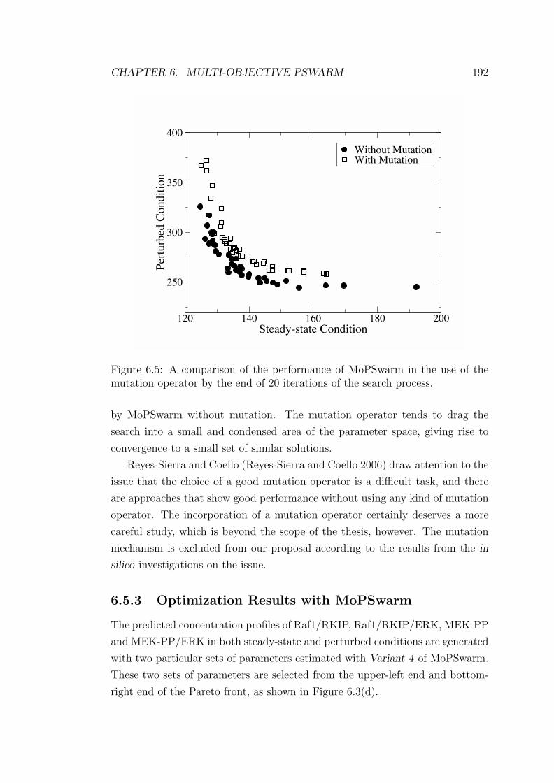
CHAPTER 7. A PROPOSED METHODOLOGICAL FRAMEWORK 246
Polyamine Concentrations (μM)
Met AdoMet dAdoMet Arg Orn Put MTA Spd
from Model 1957 18.3 3.6 118 146 785 17 614from refs. 3978 19 9 700 43 517 20 2069
Table 7.3: Polyamine concentrations considered as the basal conditions of thepolyamine model compared with those reported by Fairlamb et al. and experi-mentally measured by Mike Barrett.
is presented in Figure 7.17. Our simulations using the ‘best’ solution over an
interval of 48 hours predict well the real experimental responses, with a drastic
decrease of putrescine that caused a significant increase of dAdoMet level and a
decrease of spermidine. As expected, AdoMet is almost unchanged with a slight
decrease of the concentration level at the end of the time period. An increase of
ornithine and arginine was observed within first 12 hours of DFMO inhibition,
followed by realization of a different steady state (the arginine concentration
level stabilizes at 825 μM within a simulation interval of 72 hours).
To summarize the results of model validation with MoPSwarm, predictions
of the steady-state model and the perturbed model made using the ‘best’ so-
lution computed from the algorithm describe sufficiently well the physiological
steady-state concentrations and DFMO inhibition data. Our in silico investi-
gation further supports the biological postulation that dramatic changes in the
concentration levels of putrescine and dAdoMet are not accompanied by simi-
lar changes in AdoMet within the given time span, and arginine concentration
may not be significantly changed under the DFMO treatment. Next, we assess
the model applicability of the polyamine biosynthetic sub-pathway by examin-
ing responses to independent data sets obtained in distinct dynamic states of
the system. To the end, data from available gene perturbation experiments on
prozyme, ODC and AdoMetDC are used as validation data. In silico analysis
on some parameters of interest is also presented.
Model predictions on the effects of in vivo ODC knockdown
The similar tendencies in polyamine levels induced by DFMO inhibition are also
observed by a 90% ODC activity down-regulation. The simulation results, shown
in Figure 7.18, accurately capture the transient changes of the metabolite con-
centrations. In all figures, the experimental data measured by Xiao et al. (Xiao
et al. 2009) have been normalized to the initial concentration of the simulation

CHAPTER 7. A PROPOSED METHODOLOGICAL FRAMEWORK 247
0 500 1000 1500 2000 2500 3000Time (min)
0
5
10
15
20
25A
doM
et C
onc.
(μ
M)
Simulation DataObserved Values
(a) AdoMet
0 500 1000 1500 2000 2500 3000Time (min)
0
200
400
600
800
1000
dAdo
Met
Con
c. (μ
M)
Simulation DataObserved Values
(b) dAdoMet
0 500 1000 1500 2000 2500 3000Time (min)
0
200
400
600
800
Arg
Con
c. (μ
M)
Simulation DataObserved Values
(c) arginine
0 500 1000 1500 2000 2500 3000Time (min)
0
200
400
600
800
1000
Orn
Con
c. (μ
M)
Simulation DataObserved Values
(d) ornithine
0 500 1000 1500 2000 2500 3000Time (min)
0
200
400
600
800
Put C
onc.
(μ
M)
Simulation DataObserved Values
(e) putrescine
0 500 1000 1500 2000 2500 3000Time (min)
100
1000
10000
log
Spd
Con
c. (μ
M)
Simulation DataObserved Values
(f) spermidine
Figure 7.17: Predicted concentration profile of the perturbed model of thepolyamine biosynthetic sub-pathway. DFMO effects on polyamine levels in time-response simulations (continuous lines) are compared with experimental data(red dots). ODC concentration was modelled as a time-dependent variable. InFigure 7.17(a), AdoMet dynamics observed by Xiao et al. were adopted asexperimental data. Logarithmic axis is used for spermidine in order to betterpresent the data. Error bars are presented where appropriate data was availablein the original papers.

CHAPTER 7. A PROPOSED METHODOLOGICAL FRAMEWORK 248
data in order to better show the dynamic trend. Effects on the polyamine levels
caused by ODC activity down-regulation are smaller compared to DFMO inhi-
bition. In particular, when simulated with a DFMO treatment versus the ODC
activity down-regulation, putrescine is reduced to 0.2% versus 11% of the basal
condition, and spermidine is reduced to 49% versus 67% of the basal condition,
respectively.
0 500 1000 1500 2000 2500 3000Time (min)
0
5
10
15
20
25
30
Ado
Met
Con
c. (μ
M)
Simulation DataObserved Values
(a) AdoMet
0 500 1000 1500 2000 2500 3000Time (min)
0.001
0.01
0.1
1
10
100
1000
log
dAdo
Met
Con
c. (μ
M)
Simulation DataObserved Values
(b) dAdoMet
0 500 1000 1500 2000 2500 3000Time (min)
10
100
1000
log
Put C
onc.
(μ
M)
Simulation DataObserved Values
(c) putrescine
0 500 1000 1500 2000 2500 3000Time (min)
300
400
500
600
700
Spd
Con
c. (μ
M)
Simulation DataObserved Values
(d) spermidine
Figure 7.18: Effects of ODC knockdown on polyamine levels in time-dependentmodel simulations. In this case, ODC activity is considered a time-independentparameter. Logarithmic axis is used for dAdoMet and putrescine in order tobetter present the data. Error bars are presented where appropriate data wasavailable in the original papers.
Model predictions on the effects of in vivo AdoMetDC knockdown
and prozyme knockout
Willert and Phillips (Willert and Phillips 2008) studied the potential for prozyme
and AdoMetDC to function as regulators in polyamine biosynthesis. The authors
observed that loss of AdoMetDC or prozyme leads to decreases in spermidine and

CHAPTER 7. A PROPOSED METHODOLOGICAL FRAMEWORK 249
0 2000 4000 6000 8000Time (min)
0
1000
2000
3000
4000
5000
6000
7000
Put C
onc.
(μ
M)
Simulation DataObserved Values
(a) putrescine
0 2000 4000 6000 8000Time (min)
200
300
400
500
600
700
Spd
Con
c. (μ
M)
Simulation DataObserved Values
(b) spermidine
Figure 7.19: Effects on polyamine levels in time-dependent simulations inducedby AdoMetDC knockdown. In this case, AdoMetDC activity is considered atime-independent parameter. Error bars are presented where appropriate datawas available in the original papers.
trypanothione and to cell death. When a 70% AdoMet activity down-regulation
and prozyme knockout were applied, simulations of the polyamine model show
a dramatic increase of putrescine and a decrease of spermidine, which is in good
agreement with the tendencies described in the real experimental observations
reported by Willert and Phillips.
Simulation of the time-dependent effects on polyamine levels, putrescine
and spermidine, induced by AdoMetDC knockdown and prozyme knockout are
shown in Figure 7.19 and Figure 7.20. In both figures, the experimental data
has been normalized to the initial concentration of the simulation data in order
to better show the dynamic trend.
In our model, simulations of prozyme knockout and AdoMetDC knockdown
both resulted in a large increase in putrescine levels (approximately 7-fold in-
crease versus the 10-fold increase observed in vivo), whereas prozyme knockout
leads to a more substantial reduction in spermidine than AdoMetDC knock-
down – a 75% reduction due to prozyme knockout versus 55% reduction from
AdoMetDC knockdown. This matches well with the biological observations by
Willert and Phillips regarding the essentiality of prozyme for growth in T. brucei.
In silico simulation also indicates that an increase of putrescine as a consequence
of a 70% AdoMetDC knockdown or prozyme knockout may lead to a concomi-
tant decrease of dAdoMet and methionine; however the concentration levels of
AdoMet and arginine are largely unchanged. These model predictions can be
verified when the relevant experimental data is available.

CHAPTER 7. A PROPOSED METHODOLOGICAL FRAMEWORK 250
0 1000 2000 3000 4000 5000 6000Time (min)
0
5000
10000
15000Pu
t Con
c. (μ
M)
Simulation DataObserved Values
(a) putrescine
0 1000 2000 3000 4000 5000 6000Time (min)
0
200
400
600
800
1000
Spd
Con
c. (μ
M)
Simulation DataObserved Values
(b) spermidine
Figure 7.20: Effects on polyamine levels in time-dependent simulations inducedby prozyme knockout. In this case, the factor 1 − β representing the percentof the complex AdoMetDC|prozyme taking up the total enzyme AdoMetDC isgiven zero. Error bars are presented where appropriate data was available in theoriginal papers.
To further investigate the role that prozyme plays in the regulation of polyamine
metabolism, we performed simulations of polyamine levels with variations in the
value of β (used in Equation (7.1) and Equation (7.2)). In the model, 1 − β
accounts for the percentage of the complex compound AdoMetDC|prozyme tak-
ing up the total enzyme concentration. The value of β was assumed to vary
between 0.5 and 1 in order to reflect experimental observation and still allow
the compound to change within a physiologically feasible range. When β is
close to 1, the AdoMetDC|prozyme compound taking up the total AdoMetDC
concentration is minimal.
Figure 7.21 plots the polyamine levels obtained at the end of the simulated
time span (2880 minutes) using different values of β taken from the range [0.5, 1].
The results show that there is little effect on the polyamine levels for values of
β between 0.5 and 0.9. Significant changes in the polyamine concentrations
were observed as β approaches 1, however. The simulations indicate that the
compound AdoMetDC|prozyme accounts for a limited quantity of the total en-
zyme AdoMetDC, as the percentage of the compound taking up AdoMetDC
concentration is approximated by 1− β, where the estimated value of β is 0.94.
Prozyme reacting with AdoMetDC is a limiting factor on the AdoMetDC ac-
tivity and polyamine biosynthesis, since significant changes in polyamine levels
were only observed when the value of β falls into a small sub-range.

CHAPTER 7. A PROPOSED METHODOLOGICAL FRAMEWORK 251
0.5 0.6 0.7 0.8 0.9 1Beta
0
1000
2000
3000
4000
5000
Con
cent
ratio
n (μ
M)
putrescinespermidine
Figure 7.21: Effects of changes in parameter β on polyamine levels computed atthe end of simulation (2880 minutes): putrescine (continuous line) and spermi-dine (dashed line).
Model predictions on the effects of ‘Methylation index’
The ratio of AdoMet to AdoHcy, termed the ‘Methylation index’ indicates the
transmethylation potential of a cell (refer to Section 4.3.1 in Chapter 4). Nor-
mal methylation was shown to range from 2:1 to 9:1 (Bacchi et al. 1995). A
substantial flow from AdoMet to AdoHcy was observed in our model, with a
value of 38.9 μmol/min/mg estimated for the maximum velocity of the enzyme
AHS, which catalyzes the chemical conversion between the metabolites. Over
the simulated 48 hours of DFMO inhibition, AdoMet concentration level does
not change significantly, resulting in a constant ‘Methylation index’ (AdoHcy is
a constant model component). Our model predictions differ from the experimen-
tal observations given by Yarlett et al. (Yarlett and Bacchi 1988), which showed
that the ratio increased from 6.5 to 114 within 24 hours of DFMO treatment,
due to a large increase in AdoMet. This disagreement results from the differing
observations on the concentration of AdoMet, as observed by Xiao et al. (Xiao
et al. 2009).
Under normal conditions, a decline in the Methylation index can induce the

CHAPTER 7. A PROPOSED METHODOLOGICAL FRAMEWORK 252
so-called hypermethylation status leading to cell death (Reguera et al. 2007).
In our model, the use of AdoMet for AdoHcy production is controlled by the
maximum velocity of the enzyme AHS (V AHSmax ). Simulations of a three-fold AHS
activity up-regulation, as shown in Figure 7.22, result in a significant deple-
tion of AdoMet, dAdoMet and spermidine, accompanied by a large increase of
putrescine. The model predictions are in a good agreement with biological ob-
servations (Reguera et al. 2007) that a decline of the index reduces intracellular
spermidine level, thus leading to cell death.
0 500 1000 1500 2000 2500 3000Time (min)
5
10
15
20
Ado
Met
Con
c. (μ
M)
AdoMet
(a) AdoMet
0 500 1000 1500 2000 2500 3000Time (min)
0
1
2
3
4
dAdo
Met
Con
c. (μ
M)
dAdoMet
(b) dAdoMet
0 500 1000 1500 2000 2500 3000Time (min)
800
1000
1200
1400
1600
1800
2000
Put C
onc.
(μ
M)
putrescine
(c) putrescine
0 500 1000 1500 2000 2500 3000Time (min)
0
200
400
600
800
Spd
Con
c. (μ
M)
spermidine
(d) spermidine
Figure 7.22: Effects of a three-fold AHS activity up-regulation on polyaminelevels in time-dependent model simulations.
Yarlett et al. (Yarlett et al. 1991) found that in T. brucei, transmethylation
reactions were very sensitive to AdoHcy inhibition. Figure 7.23 shows the effect
of apparent inhibition value KAHSiAdoHcy (representing the AdoHcy inhibition on the
enzyme AHS) on AdoMet and dAdoMet intracellular concentrations. AdoMet
concentrations simulated at the final time point of the time span 0 to 48 hours
were plotted. These are calculated using values of KAHSiAdoHcy taken from the range
0.01–2 fold the observed value of 12.9 μM. Our model predicts a gradual reduc-

CHAPTER 7. A PROPOSED METHODOLOGICAL FRAMEWORK 253
0 5 10 15 20 25 30Apparent inhibition (μM)
0
5
10
15
20
25
30
35
Ado
Met
Con
c. (μ
M)
AdoMet
(a) AdoMet
0 5 10 15 20 25 30Apparent inhibition (μM)
0
200
400
600
800
dAdo
Met
Con
c. (μ
M)
dAdoMet
(b) dAdoMet
Figure 7.23: Effects of changes in AHS enzyme related apparent coefficient on theconcentration levels of AdoMet and dAdoMet computed at the end of simulation(2880 minutes). The coefficient varies in the range of 0.01–2 fold of the observedvalue.
tion in the final AdoMet level as the apparent inhibition coefficient increases,
followed by a rapid depletion of dAdoMet. There is, however, no experimental
data available to verify the predictions.
7.9.4 Remarks on the Mathematical Model
We have demonstrated in this section that the proposed mathematical model is
an adequate representation of the system of polyamine metabolism. This allows
various types of analysis methods to be applied to the model. For example,
Metabolic Control Analysis (MCA), as defined by Cascante et al. (Cascante
et al. 2002), provides a quantitative description of system variables (i.e. fluxes
and metabolite concentrations) in response to changes in system parameters.
With this method, the relative control exerted by each step (enzyme) in the
polyamine pathway on the system variables can be assessed and the enzymatic
reactions that have the greatest influence on the regulation of polyamine func-
tion and metabolism can be identified. Our mathematical model also offers
opportunities to investigate different strategies for targeting this pathway in
anti-trypanosomal drug design. For instance, an effective treatment of human
African trypanosomiasis could be achieved by enhancing polyamine depletion via
combined blockage of polyamine synthesis. With such information, promising
targets for anti-protozoal agents can be proposed or less promising possibilities
can be eliminated. The details of such analyses are beyond the scope of the
thesis.

CHAPTER 7. A PROPOSED METHODOLOGICAL FRAMEWORK 254
7.9.5 Structural Modelling vs. Kinetic Modelling
One of the aims of structural modelling is to predict the relative fluxes of all
internal reactions in the system via optimization of a specific objective function
(see Section 3.5.1 in Chapter 3). The steady-state reaction flux distribution
in a metabolic pathway predicted by the mass-balance model can be compared
quantitatively to the fluxes predicted by the kinetic model.
Table 7.4 reports the steady-state flux distribution in the polyamine biosyn-
thetic sub-pathway computed by both approaches. The fluxes going though the
reactions determined by the kinetic model (the corresponding rate equations are
given in Table 7.2) are approximated with the ‘best’ set of parameters. Note
that the flux through the reaction step of exogenous methionine assimilation
has a known value of 0.122 μmol per min per mg of cell protein, calculated by
Equation (4.19) in Chapter 4.
The structural model of the polyamine biosynthetic sub-pathway can be ex-
tracted from matrix (3.12) (defined in Chapter 3). Irrelevant metabolites and
reactions to this sub-pathway are removed, which causes the accidental removal
of an essential reaction step concerned with AdoMet-dependent transmethyla-
tion. To make the model consistent with the schematic representation of the
sub-pathway (see Figure 7.13), the reaction step of AdoHcy production from
AdoMet is introduced (AdoHcy is set as an additional external metabolite) and
a new output reaction describing the conversion of spermidine into trypanoth-
ione biosynthesis (catalyzed by Spdout) is also added.
The reaction flux going through the step of spermidine consumption into try-
panothione biosynthesis is defined as the objective function, in order to allow the
two modelling approaches to be compared. The steady-state flux distribution of
the sub-pathway via structural modelling is obtained by maximizing this objec-
tive function. The flux of the input reaction – exogenous arginine assimilation
– is not available from the literature, and the value approximated by the kinetic
model is assigned to this reaction flux. The flux of the other input reaction –
exogenous methionine assimilation – is fixed as given above. All the internal
reaction fluxes are assumed to vary between 0 and 2, with units of μmol per
min per mg of cell protein. The maximum flux through the objective function
(reaction index 10 in Table 7.4) is constrained with the corresponding flux value
predicted by the kinetic model.
Table 7.4 shows a good match between the predictions from structural mod-
elling and kinetic modelling. The internal fluxes predicted by optimizing the

CHAPTER 7. A PROPOSED METHODOLOGICAL FRAMEWORK 255
Index Reaction Name Stoichiometry SM KM1 Arginase arginine → ornithine 0.7275 0.72752 Ornithine decarboxylase ornithine → putrescine 0.7275 0.72803 AdoMet synthase methionine → AdoMet 0.8500 1.15844 AdoMet decarboxylase AdoMet → dAdoMet 0.7275 0.72805 AdoMet-dependent AdoMet → AdoHcy 0.1220 0.4287
transmethylation6 Spermidine synthase putrescine+dAdoMet 0.7275 0.7301
→ spermidine+MTA7 MTA recycling MTA → methionine 0.7275 0.73018 Arginine assimilation Extarg → arginine 0.7275 0.72759 Methionine assimilation Extmet → methionine 0.1220 0.122010 Spermidine consumption spermidine → 0.7275 0.7386
trypanothione biosynthesis
Table 7.4: Comparison of the steady-state flux distributions in the polyaminebiosynthetic sub-pathway predicted via structural modelling and kinetic mod-elling. All the values are expressed in the units of μmol per min per mg ofcell protein. SM and KM stand for the structural model and kinetic model,respectively.
structural model are almost identical to the fluxes computed with the kinetic
model and the objective function is optimized sufficiently close to the maximum
value (0.7275 versus 0.7386).
Fluxes going through the reaction steps – AdoMet synthase and AdoMet-
dependent transmethylation – were solved with different values. This can be
explained from numerical aspects. AdoMet is a branching point in the polyamine
biosynthetic sub-pathway, where one incoming reaction (reaction 3) is split into
two outgoing reactions (reaction 4 and 5). In this case, when only one flux is
known, in theory, there will be many combinations of flux values to be computed
for the other two reactions, and therefore values of these fluxes can only be
determined based on constraints imposed by other fluxes.
When solving both models, the reaction step describing the conversion of
methionine into AdoMet (reaction index 3 in Table 7.4) is predicted to carry the
maximum flux value of all the internal reactions, indicating the significant role
that this reaction step plays in satisfying the objective function. This observation
is consistent with the analysis results of control-coefficient fluxes representing
the importance of each reaction for efficient and flexible operation of the entire
pathway. As shown in Figure 3.10 in Chapter 3, of all the polyamine reactions,

CHAPTER 7. A PROPOSED METHODOLOGICAL FRAMEWORK 256
the reaction of interest (reaction 3) is calculated with the highest control-effective
flux (Note that in the figure reactions 1–7 and 15–16 correspond to reactions 1–9
in Table 7.4).
In summary, with appropriate constraints, a good interpretation of the metabolic
capacities of the polyamine biosynthetic sub-pathway can be obtained by opti-
mizing the structural model with respect to a specific objective function. The
consistency of predictions of internal reaction fluxes in both types of models
gives confidence that the models are an adequate reflection of the real system,
given the absence of experimental data. With the predicted metabolic fluxes, an
adequate measure of the degree of participation of the polyamine biosynthetic re-
actions in the process of spermidine participation in trypanothione biosynthesis
is obtained.
7.9.6 Computational Issues
MoPSwarm is a reliable and efficient multi-objective optimization algorithm.
From the modelling point of view, model validation with MoPSwarm is a promis-
ing strategy. The present model structure combined with estimated parameter
values is able to consistently interpret the underlying biological processes. This
is ascribed to the fact that MoPSwarm allows an integrated study of different
states of the polyamine biosynthetic sub-pathway, which is an essential condition
for the elucidation of regulatory principles. In the context of parameter estima-
tion, MoPSwarm enables non-dominated solutions covering a well-distributed
Pareto front to be found with a small population of particles (20 initial parti-
cles) and with a small number of generations (less than 1000 generations). The
proposed algorithm is not only able to optimize problems exhibiting straight-
forward convex tradeoffs but also addresses problems resulting discontinuous
Pareto fronts.
Due to the sparse nature of the problem, it is frequently difficult for the
ODE solver to integrate the differential equations. Some regions of the param-
eter space are numerically unstable and the solver may stall or produce invalid
results, such as NaNs (Not a Number) and integration failures. It is necessary to
implement error handlers in MoPSwarm to deal with these problems; the Matlab
solver ode15s was modified to include an extra error handler to prevent stalling
due to invalid results. For a difficult optimization problem, such as this, we
replaced ‘2× fi(x)’ with ‘10× fi(x)’ in the mathematical definition of ‘Partially

CHAPTER 7. A PROPOSED METHODOLOGICAL FRAMEWORK 257
Dominated Solutions’ (see Definition 6.5 in Chapter 6); that is, a particle may
be up to 10x as bad in any one objective if there is any improvement in the other.
This was designed to prompt a good diversity in the Pareto-optimal solutions
by easing the strict constraint imposed on the selection of ‘good’ particles.
During the search process, MoPSwarm was frequently confronted with diffi-
cult search regions with many invalid positions found for both the steady-state
and perturbed model. For example, in the course of identifying the Pareto front
shown in Figure 7.15, MoPSwarm retrieved only 28 trade-off solutions in the pa-
rameter search space with variations in the parameter values covering 5 orders of
magnitude, with 3145 and 2441 invalid results found for the steady-state model
and the perturbed model, respectively. This may explain why the resulting ap-
proximate Pareto-optimal front is concave and discontinuous, being comprised
of four disconnected Pareto-optimal sets and a single point.
Despite the good results achieved by MoPSwarm, the number of fitness func-
tion evaluations may be very large, and the computational cost of using this
approach can vary significantly when solving other systems. The most likely
cause of this is from variations in the time taken to evaluate the model in order
to determine the objective function value. In our case, the average computation
time over ten simulation runs of model validation is approximately 19 hours on
AMD Opteron 2000-based cluster nodes.
7.10 Conclusions
Mathematical modelling of biological systems involves the identification of chem-
ical relations between system components and the formulation of kinetic mecha-
nisms representing the enzymatic catalysis. Constructing a detailed mechanistic
model for the trypanothione metabolic pathway is a challenging task for several
reasons:
• First, the system is ambiguously determined in terms of both network
topology (chemical relations between system components) and kinetic char-
acters (rate laws governing the reaction velocities). A systematic identifi-
cation procedure for model structure correctness is necessary.
• Second, the search space is very complex in terms of both scale and di-
mensionality. Feasible region(s) – where optimal solutions are located in
the search space can be very small and the search can be complicated by

CHAPTER 7. A PROPOSED METHODOLOGICAL FRAMEWORK 258
the existence of infeasible region(s) where no solutions can be achieved and
the system may be numerically unstable.
• Third, the very limited number of experimental observations imposes a
significant challenge to optimization methods. Parameter estimation is
particularly difficult when the dimensionality of parameters to be resolved
is much larger than the number of measurement samples.
In this chapter, we proposed a methodological framework (Figure 7.1) in or-
der to tackle the challenge imposed by data sparsity and incompleteness of prior
knowledge of the system. The purpose of the proposed framework is to reduce
the whole system into sub-systems through an iterative process and then study
the sub-systems in a modular manner, which supports the model refinement
in a functionally independent manner. Module-based representation allows the
understanding of the entire system through parsing the sub-systems that are
smaller in terms of both the number of state variables and kinetic parameters,
by means of which complexity of the original system can be largely reduced.
Module-based representation is thereby a very useful strategy in the develop-
ment of mathematical models for large-scale non-linear dynamic systems.
One major difficulty of system identification lies in the design of correct
model structures to consistently interpret the underlying processes, which in-
volves seeking missing reactions or refining ill-characterized kinetic mechanisms.
When no or limited biological evidence is given, it is almost impossible to make
biologically meaningful assumptions about suitable model structures. The de-
sign principle of model decomposition in the proposed methodological framework
is to direct the search for ill-characterized kinetic characters of the pathway in
an efficient manner. This methodological framework has the potential to solve a
wide range of cellular processes, including gene regulatory pathways, signalling
pathways and metabolic pathways.
The procedure for model structure exploration does not lead to verification of
models; rather to their falsification. Given conflicting experimental data, differ-
ent mathematical models are expected, which may also show major variations
due to imprecise measurements. It of course must also be remembered that
proposed model structures are consistent in describing the biological data only
within limits of experimental noise and the biological phenomena modelled.
By applying the proposed methodological framework, a novel kinetic model of
the polyamine biosynthetic sub-pathway is successfully constructed. The module

CHAPTER 7. A PROPOSED METHODOLOGICAL FRAMEWORK 259
predicability is preserved by using the Hill function to approximate the mod-
ule interaction with the rest of the pathway. The regulatory principles of the
polyamine biosynthetic sub-pathway were elucidated by studying the system in
different physiological states. The agreement between model simulation with the
estimated parameter values and measured data reported in various experimental
conditions shows the good applicability of the kinetic model of the sub-pathway.
The system behaviour that has not yet been observed was also predicted by in
silico model simulations. We observed an abrupt change on the polyamine levels
in response to a gradual decrease of the complex compound – AdoMetDC|prozyme
within a physiological range of the AdoMetDC concentration. A regulatory link
between the polyamine enzymes was predicted to be an essential feature for
arginine metabolism, as inferred from model simulation. An enzyme assay could
be designed to verify the prediction by determining the arginine transport rate
and arginase activity in T. brucei mutants that lack or are deficient in ODC.
The regulatory link can be verified if suppression of arginine transport rate and
arginine activity is observed.

Chapter 8
Conclusions and Future Work
In this thesis, the challenges associated with the computational modelling of
complex biological systems when prior knowledge was restricted by sparse quan-
titative information and incomplete physical descriptions of the underlying pro-
cesses have been investigated. In this chapter we summarize the main points
of the work and reiterate the contributions drawn. We also discuss interesting
future work directions, including possible improvements and extensions on the
proposed approaches.
8.1 Conclusions
A systematic approach is necessary to elucidate the complex relationships involv-
ing multiple system components governed by non-linear kinetics. The emerging
field of Systems Biology provides a powerful foundation and established scientific
methods to enable the study of biological pathways at the system level.
In biology, the identification and understanding of system behaviour is not an
easy task. The difficulty in achieving a system-level understanding stems from
the intrinsic complexity of biological systems where large numbers of functionally
diverse components interact non-linearly. It has been widely accepted that the
best way to understand complex networks of biological pathways is via the use
of computational modelling. However, this is often complicated by incomplete
prior knowledge of the system. Inconsistent and sparse experimental data of the
network also creates a multitude of problems for the modelling process.
Constructing a sound mathematical model to understand biological systems
is a challenging endeavor. Mathematical models with a high degree of precision
and quality are necessary for drug discovery and treatment optimization, where
260

CHAPTER 8. CONCLUSIONS AND FUTURE WORK 261
multiple aspects of the biological processes have to be integrated and the model
predictions must be validated with the experimental observations. Mathematical
modelling is also a useful tool for the development of new processes and in this
case has allowed disparate information about the system to be organized and
represented in a coherent manner.
Chapter 4 contributes to knowledge of the first detailed kinetic model of an
important biological system – the trypanothione metabolic pathway in the proto-
zoan parasite Trypanosoma brucei. We focused on continuous and deterministic
descriptions of the trypanothione metabolism by using non-linear ordinary dif-
ferential equations. We took into account the essential information in order to
build a useful mathematical model. An extensive literature search about the
metabolic pathway was conducted, where scientific papers relevant to individual
enzyme kinetic properties were critically reviewed.
We have proposed a new methodological framework to address the mod-
elling challenges and illustrated the feasibility of the framework by studying the
trypanothione metabolic pathway in Trypanosoma brucei. Metabolism in this
parasitic organism is the focus of several investigations for anti-trypanosomal
therapeutics, as Trypanosoma brucei remains a major problem in developing
countries despite the availability of several drugs. To achieve the goals, some
existing scientific methods have been reviewed and then adapted and extended
in an appropriate way for use in solving the problem of interest.
8.1.1 Metabolic Modelling
As stated in Chapter 1, the type of model should depend on the biological sys-
tem in question, the type/amount of information available and the intended use
of the model. A system-level understanding of the trypanothoine metabolism
has been attempted through structural and kinetic modelling approaches. Both
approaches are essential to understand the metabolic properties of the path-
way and focus on topological and regulatory properties, respectively. Structural
modelling and kinetic modelling are complementary approaches, and one enables
a determination of a variety of model properties that could not be allowed by
the other.
Knowledge about the trypanothione metabolic pathway is currently restricted
to a qualitative view and the network topology is better understood than its nu-
merical aspects. Most of the cellular enzymes, such as regulatory mechanisms

CHAPTER 8. CONCLUSIONS AND FUTURE WORK 262
are, at best, qualitatively known; detailed enzyme-kinetic models are lacking.
This creates severe difficulties for kinetic modelling of the pathway in order to
comprehend the trypanothione metabolism in its entirety, which was demon-
strated in Chapter 7. In the absence of enough kinetic information, structural
modelling is one promising approach for the understanding the trypanothione
metabolism as a whole.
Chapter 3 reported the first structural model of the trypanothione metabolic
pathway. In this chapter, we applied a theoretical structural modelling approach
to study the network metabolism even in the absence of sufficient quantitative
information of target enzymes. This structural modelling approach is based on
the stoichiometry and the reversibility of the metabolic reactions, which is a
structural invariant of the pathway, and uses theoretical tools to investigate the
model. Topological properties and metabolic capabilities of the trypanothione
pathway to support cell growth were investigated with this approach. Essential
genes were predicted by optimizing the mass-balance model of the pathway with
respect to given objective functions (biomass yield and H2O2 residual).
By structural modelling, we computationally tested the completeness of avail-
able topological information based on the elementary mode analysis. When the
metabolic flux measurements become available and adequate, the postulated ad-
ditional reactions of the pathway can be verified. We examined the consistency of
given objective functions for linear programming with experimentally observed
genotypes. Wrong predictions revealed an incorrect definition of the objective
functions, improving our understanding of the growth control of trypanosomes.
Two constituting factors of the trypanosomal growth are characterized with two
topological modules carrying out specific metabolic functions – the trypanoth-
ione biosynthetic system and the trypanothione redox system.
Although the structural model was not used for simulation, it still helped
us focus on the essential features of the system and facilitated the construction
and simplification of the kinetic model of the pathway. This type of modelling
enabled an establishment of the correlation between topological modules (spa-
tially isolated) and functional modules (carrying out a monotonous metabolic
function), which is otherwise not easy to achieve. This information was used to
aid the initialization of model decomposition in the methodological framework
proposed in Chapter 7.
Application of structural modelling to the trypanothione metabolic pathway
provided us a relatively simple starting point to understanding the approach.

CHAPTER 8. CONCLUSIONS AND FUTURE WORK 263
The work performed demonstrates the feasibility of structural modelling for un-
derstanding the system when it extends to the genome level. The predictions
of the steady-state flux distribution in the polyamine biosynthetic sub-pathway
from structural modelling and kinetic modelling were compared with appropriate
constraints. Since the measurement of fluxes is a tedious task, the good agree-
ment of both models indicates that the models are adequate representations of
the real system.
However, flux distributions under steady-state conditions do not explain any-
thing about the regulatory principles of the system and the disadvantage of
structural modelling is that dynamical aspects of the systems are left implicit.
We have demonstrated in Chapter 4 and further discussed in Chapter 7 that a
realistic metabolic model, using coupled enzymatic reactions, can only be de-
scribed by a system of non-linear equations for which no analytical solutions can
be easily obtained.
8.1.2 Optimization of Computational Models
Chapter 5 laid the foundation for the optimization-based study, which played
an essential role in the methodological framework proposed in Chapter 7. This
chapter reviewed some of the basic theory associated with optimization and dis-
cussed Particle Swarm global optimization and the derived PSwarm algorithm.
PSwarm is a recently developed population-based optimization method and has
not yet been widely applied to biological problems. This chapter investigated the
performance of the algorithm, which demonstrated that PSwarm is capable and
efficient in tackling the inverse problem of complex biological systems. PSwarm
was employed as the search engine during the examination of model structural
correctness. The problem of parameter estimation suffering from missing exper-
imental measurements and lack of information content was illustrated using the
ERK signalling pathway.
Chapter 6 proposed a novel approach MoPSwarm for applying a multi-
objective optimization to the validation of perturbation-based models of bio-
logical systems. MoPSwarm is a generalized pattern search algorithm, defined
by a Search-and-Poll framework, where the standard particle swarm optimiza-
tion is employed in the search step and the poll step is only activated when the
search step failed. Satisfactory simulation results of the ERK signalling path-
way using the proposed validation approach demonstrated the reliability and

CHAPTER 8. CONCLUSIONS AND FUTURE WORK 264
utility of the proposed algorithm for model validation in comparison with the
conventional approach. This chapter, combined with the work on the algorithm
presented in Chapter 7, indicated that model validation is the most difficult
problem in the modelling process, particularly when the model predicability is
reliant on accurate and reliable quantification of parameters.
Despite the great challenge in solving the real-world applications (includ-
ing the ERK signalling pathway and the polyamine biosynthetic sub-pathway)
due to their non-linear nature, MoPSwarm has shown good performance in tack-
ling multi-objective optimization problems characterized with various properties.
Experimental results from model simulation of both biological pathways demon-
strated that MoPSwarm enables us to find non-dominated solutions covering a
wide-spread Pareto front with a small number of population (20 initial particles)
and with a small number of generations (less than 1000 generations).
Multi-objective optimization simultaneously takes several, possibly conflict-
ing aspects into consideration. We have demonstrated that with the multi-
objective optimization scheme, a population of solutions results from a single
run of the algorithm owing to the contradictory objectives and several parts of
the objective space can be explored simultaneously. A practical interpretation
of the Pareto-optimal front is that different solutions can be selected to describe
the system according to the degree of confidence ascribed to individual objective.
We have performed a comparative study investigating some of the factors
important to the performance of MoPSwarm in solving multi-objective opti-
mization problems. We have found that the choice of selection scheme for global
best guide and the mechanism for updating the archive is critical for the Pareto-
based approach, from the perspective of promoting an effective search towards
the Pareto front and maintaining diversity in the population. Experimental
investigation indicated that MoPSwarm is capable of tackling the multi-modal
objective function space. The proposed algorithm is not only able to detect solu-
tion spaces exhibiting straightforward convex tradeoffs but also address concave
and discontinuous Pareto fronts. By simultaneously optimizing the steady-state
and perturbed model, the difficulty of potentially large steady-state degrees of
freedom can be relieved by incorporating time-depedent system dynamics. Com-
putational investigations of MoPSwarm underlined the necessity of considering
more than one state of the system for reliable parameter estimation.

CHAPTER 8. CONCLUSIONS AND FUTURE WORK 265
8.1.3 Computational Modelling
The proposed methodological framework is envisioned as an important contribu-
tion to the mechanism-based mathematical modelling of complex biological sys-
tems. The novelty lies in the integration of mathematical modelling (analytical
approach) and system identification (experimental approach) to enable physical
insights about the system to be accounted for in the modelling procedure, partic-
ularly when our prior knowledge is restricted. By means of the methodological
framework, the mathematical model of the trypanothione metabolic pathway
initially described in Chapter 4 was explored strategically.
We have carried out in this thesis one of the few works on studying model
inappropriateness. Mismatch between the model responses given a certain struc-
ture and experimental observations via the optimization-based study with PSwarm
has uncovered the inappropriateness in the model representation.
A major biological use of this work would be to generate predictions about
enzyme kinetics and regulatory mechanisms to be tested by in vivo approaches.
Since mathematical models are manipulable, the basic principles of metabolic
regulations via different kinetic characters can be evaluated. Data produced in
silico combined with collections of in vivo experiments motivate the formula-
tion of new hypotheses to be placed in computational experiments for testing
and validation. The regulatory link between the polyamine enzymes, includ-
ing exogenous arginine transporter, arginase and ODC has been hypothesized
and validated via in silico model simulation that is amenable to further biolog-
ical studies. After biological experiments have been performed for hypothesis
verification, models can be iteratively improved and new insights can be gained.
The significance of model decomposition in the early stage of computational
modelling has been underlined. The module-based model presentation has al-
lowed us to focus on comparatively well-characterized modules and to study
the poorly-defined sub-systems when the relevant biological information is ade-
quate for a mechanism-based model construction. The model decompositional
approach assisted in an effective identification of the possible ill-characterized
reactions without detailed biological information being available.
In terms of computational modelling, the module-dependent study allowed
the selection of appropriate model representations to elaborate the underlying
processes of the system described by different amounts of relevant prior knowl-
edge. The usefulness of characterizing different parts of the system with different
mathematical model representations has been demonstrated in the computa-

CHAPTER 8. CONCLUSIONS AND FUTURE WORK 266
tional modelling of the polyamine biosynthetic sub-pathway in Chapter 7 – the
enzymatic reactions for spermidine production were modelled based on detailed
physical insights and spermidine participation in the rest of the trypanothione
metabolic system was approximated with a non-linear regression function. From
the optimization point of view, module-based representation simplified the math-
ematical description of the system by approximating ambiguously-characterized
sub-systems with a parametric function, reducing the degrees of freedom of the
parameters to be estimated.
Understanding complex biological systems on the basis of functional modules
enables flexible system models to be built from reusable components and allows
different calculations to be employed for these components. Module-based mod-
els can also assist the analysis of similar modules in related species (e.g. in T.
brucei, Leishmania and T. cruzi) to identify mutually-shared or species-specific
functions.
The model of polyamine biosynthetic sub-pathway developed in this thesis
has enabled a scientific explanation of measured data and a consistent interpre-
tation of the underlying biological processes. We have shown that our model
of polyamine interconversion reflects some critical features observed in experi-
mental approaches, such as ODC knockdown, AdoMetDC knockdown, prozyme
knockout and variations in the Methlyation index. The modelling activities per-
formed on the trypanothione metabolic pathway have great potential to help
experimentalists clarify conceptual ambiguities and to provide a platform for
rational identification of potential anti-trypanosomal druge targets.
8.2 Future Work
There are several areas for possible improvements and extensions on the work
presented in this thesis.
The first suggestion for future research work is the investigation of
the trypanothione metabolism in Trypanosoma brucei on the genomic
scale. Reconstruction of the metabolic network of the parasite Leishmaina ma-
jor has recently been reported by Chavali et al. (Chavali et al. 2008). The
work in Chapter 3 and Chapter 4 provides an opportunity for the genome-scale
construction of the metabolic network in the parasite Trypanosoma brucei. To
achieve the goal, a variety of data sources must be integrated in order to ex-
pand the existing structural model, including available genomic, proteomic and
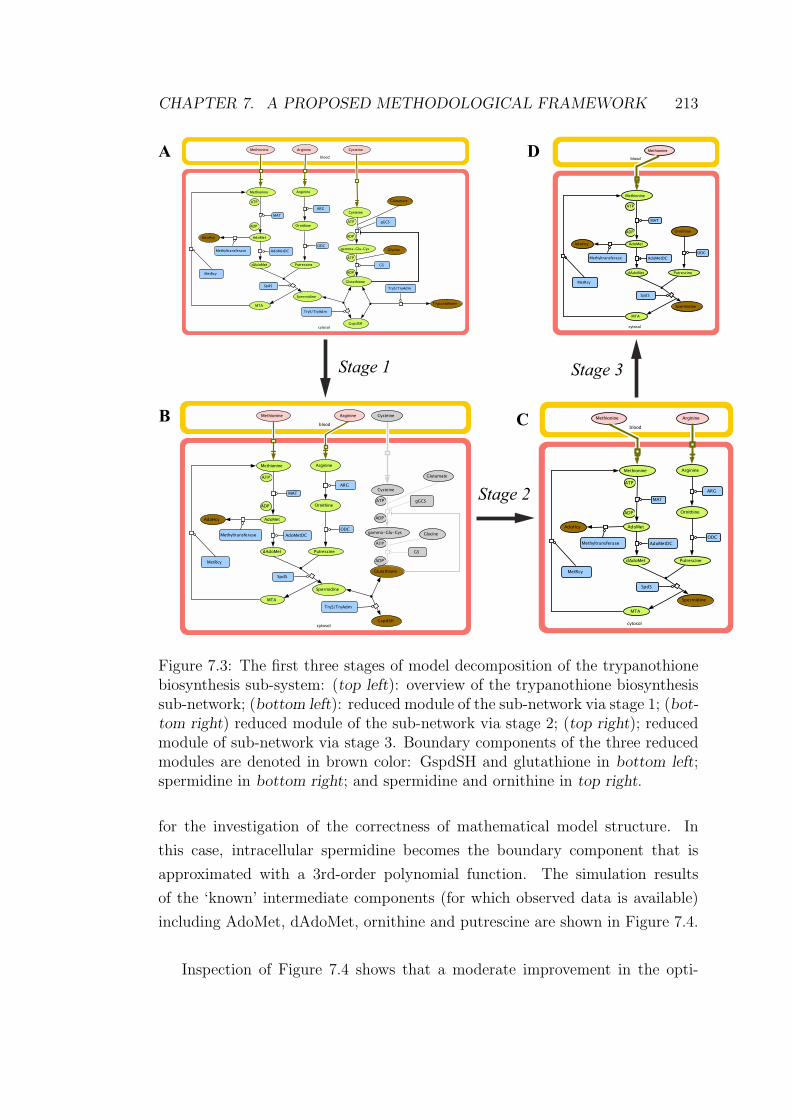
CHAPTER 8. CONCLUSIONS AND FUTURE WORK 267
metabolomic data. The computational modelling and systems analysis meth-
ods described in Chapter 3 could be readily applied to the future study of this
parasitic organism.
The second suggestion for future research work is the integration
of structural model and kinetic model of the trypanothione metabolic
pathway in order to build a whole-cell model. We have emphasized the
importance of structural modelling and kinetic modelling as individual mod-
elling approach for studying metabolic pathways. A strategy of integrating the
structural and kinetic models appears to be prevalent in practice. Recently, a
framework that combines models of different types of biological processes (e.g.
metabolic and regulatory processes ) was developed by Covert et al. (Covert
et al. 2008) for building whole-cell models. Their framework requires the avail-
ability of different models (e.g. structural model and kinetic models) of the same
system in order to create an integrated model. Our work in Chapter 3, Chapter 4
and Chapter 7 developed the structural model and tackled the construction of
kinetic model for T. brucei, making the proposed framework by Covert et al.
suitable for application to the development of a whole-cell model in T. brucei.
As their approach demands a complete description of the initial conditions
of biomass, enzymes and metabolites of the system, a number of in vivo ex-
periments must be performed in order for their approach to be useful. A good
starting point of future research would concentrate on the model of polyamine
biosynthetic sub-pathway, for which some unknown parameters have already
been estimated with MoPSwarm. An interesting question to address could be
concerned with studying the regulation between AdoMetDC and prozyme of
the polyamine sub-pathway. The regulatory mechanism of the two enzymes has
been postulated via the kinetic modelling in Chapter 4. However, the postulated
mechanism cannot be tested due to the lack of measured dynamics essential for
the purpose. We expect that by integrating the kinetic model with the struc-
tural model of the polyamine biosynthetic sub-pathway, more knowledge could
be gained for this regulatory mechanism.
The third suggestion for future research work is a parallel imple-
mentation of the multi-objective optimization algorithm MoPSwarm
for increased computational speed. To increase the usefulness of the MoP-
Swarm proposed in this thesis, a potential enhancement to the computational
efficiency of the algorithm is suggested. The Poll step is an important strategy
adopted in the algorithm to guarantee satisfactory convergence to stationary

CHAPTER 8. CONCLUSIONS AND FUTURE WORK 268
points and a good diversity of the Pareto-optimal solutions. However, the num-
ber of evaluations of fitness functions in the Poll step may be very large and the
computational cost of using this approach can vary significantly when solving
other systems.
A parallel implementation of the algorithm would be a good solution for
improving the computational speed. An attempt has been made to parallelize
Particle Swarm for application to computationally demanding single-objective
optimization problems (Schutte et al. 2003). Other general strategies could be
parallelization onto multiple processors using an interface such as MPI (message
passing interface – http://www.open-mpi.org/) or parallelization onto hardware
accelerated platform such as GPUs.
The fourth suggestion for future research work is the enhancement
of the algorithm MoPSwarm for tackling multi-objective optimization
problems. Although MoPSwarm as designed in this thesis in general aims at
solving optimization problems constrained by multiple objectives (more than two
objectives), the focus has been given to solving problems with two objectives.
The requirement to enhance the generalization of MoPSwarm mandates further
work on designing appropriate mechanisms in selecting trade-off solutions among
objective functions. This may involve assigning different ‘weights’ to individual
objective as importance factors when they are simultaneously solved. MoP-
Swarm is a stand-alone algorithm and only requires mathematical model (e.g
ODEs) and objective functions (e.g. least squares) as inputs, which facilitates
future enhancement of the algorithm.
The final suggestion for future research work is the adaptation
of the methodological framework for automatic computational mod-
elling. The methodological framework proposed in Chapter 7 intends to tackle
the problem of structure identification caused by ill-defined kinetic mechanisms
of reaction enzymes, since in most cases the network topology is better under-
stood than regulatory mechanisms. This framework is fundamentally a heuristic
approach, where modeller’s interactions with the framework in each phase are
necessary. Automatic modelling procedure would be appealing in practice, par-
ticularly for extreme cases, where no biological information concerning either
network topology or kinetic mechanisms is obtainable for in silico investigation
of system identification problems.
We envision that automation of the modelling methodology could be achieved
via a bilevel architecture. The outer level searches through a library of reactions

CHAPTER 8. CONCLUSIONS AND FUTURE WORK 269
and/or enzyme kinetics to include so that model simulation can agree with ex-
perimental data given a particular model structure. An appropriate (qualitative
or quantitative) measure of the level of agreement between model simulation and
system responses is crucial for determining ‘good’ structures. The inner level
deals with the problem of model validation for the structure(s) that passed the
outer level examination, in which case MoPSwarm can be employed.
However, to make the automated procedure useful, certain issues should be
taken into account. One issue is that models without biological interpretation
could be derived. Much attention has to be paid in the selection of suitable
model structures and models without biological support should not be included
in the set of candidate models. Another issue is that computational cost can be
enormous with increasing model complexity. This difficulty could be relieved by
incorporating expert knowledge about ‘good’ parts of the model structure, and
focusing on only suspected system characteristics during the procedure.

Appendix A
Experimental Data
This section reports the experimental observations that are used for the study
in Chapter 7. This data includes DFMO-treated drug responses and single-gene
knockdown profiles. Intracellular concentrations of the metabolites are given in
μM that are caculated based on a volume of 58 μL/109 trypanosomes (Opperdoes
et al. 1984).
A.1 DFMO-treated Drug Responses
Table A.1 summarizes the effect of DFMO on bloodstream-form T. brucei (Fairlamb
et al. 1987) and Table A.2 the effect on procyclic form T. brucei (Bellofatto
et al. 1987).
Metabolites Wt Wt+DFMO Wt+DFMO Wt+DFMO12hrs 36hrs 48hrs
ornithine 43 759 759 569putrescine 517 3.3 3.3 3.3AdoMet 19 34 1069 1431dAdoMet 9 34 397 793Spermidine 2069 948 845 517GspdSH 48 34 31 29glutathione 234 397 414 397trypanothione 340 257 207 116
Table A.1: Dynamic responses of the intracellular metabolite concentrations inbloodstream-form T. brucei. Wt (wild-type) and Wt+DFMO stand for intra-cellular concentrations at the steady state and under drug inhibition.
270

APPENDIX A. EXPERIMENTAL DATA 271
Metabolites Wt Wt+DFMO Wt+DFMO Wt+DFMO12hrs 36hrs 48hrs
arginine 603 862 1293 1896ornithine 43 2069 2069 2069putrescine 2931 258 0 0dAdoMet 0 172 431 603Spermidine 3793 2758 1465 1034GspdSH 77 34 34 34glutathione 465 552 862 1000trypanothione 672 431 379 310
Table A.2: Dynamic responses of the intracellular metabolite concentrations inprocyclic-form T. brucei. Wt (wild-type) and Wt+DFMO stand for intracellularconcentrations at the steady state and under drug inhibition.
A.2 Single-gene Knockdown Profiles
Table A.3 summarizes the effects of SpdS (spermidine synthase) knockdown on
the intracellular metabolite concentrations in T. brucei (Xiao et al. 2009).
Metabolites Wt Wt+Tet Wt+Tet Wt+Tet12hrs 36hrs 48hrs
putrescine 869 517 445 245dAdoMet 0.07 2.24 7.07 10.7Spermidine 1548 881 407 366GspdSH 11.2 1.2 3 1e-3glutathione 164 188 198 210trypanothione 2.6 2.2 2.6 3.4e-2
Table A.3: The effects of SpdS knockdown on the intracellular metabolic concen-trations in bloodstream-form T. brucei. Wt and Wt+Tet stand for intracellularconcentrations at the steady state and after Tet induction. The addition of Tet(tetracycline) degrades the target enzyme, essentially knocking it down by agiven fraction.
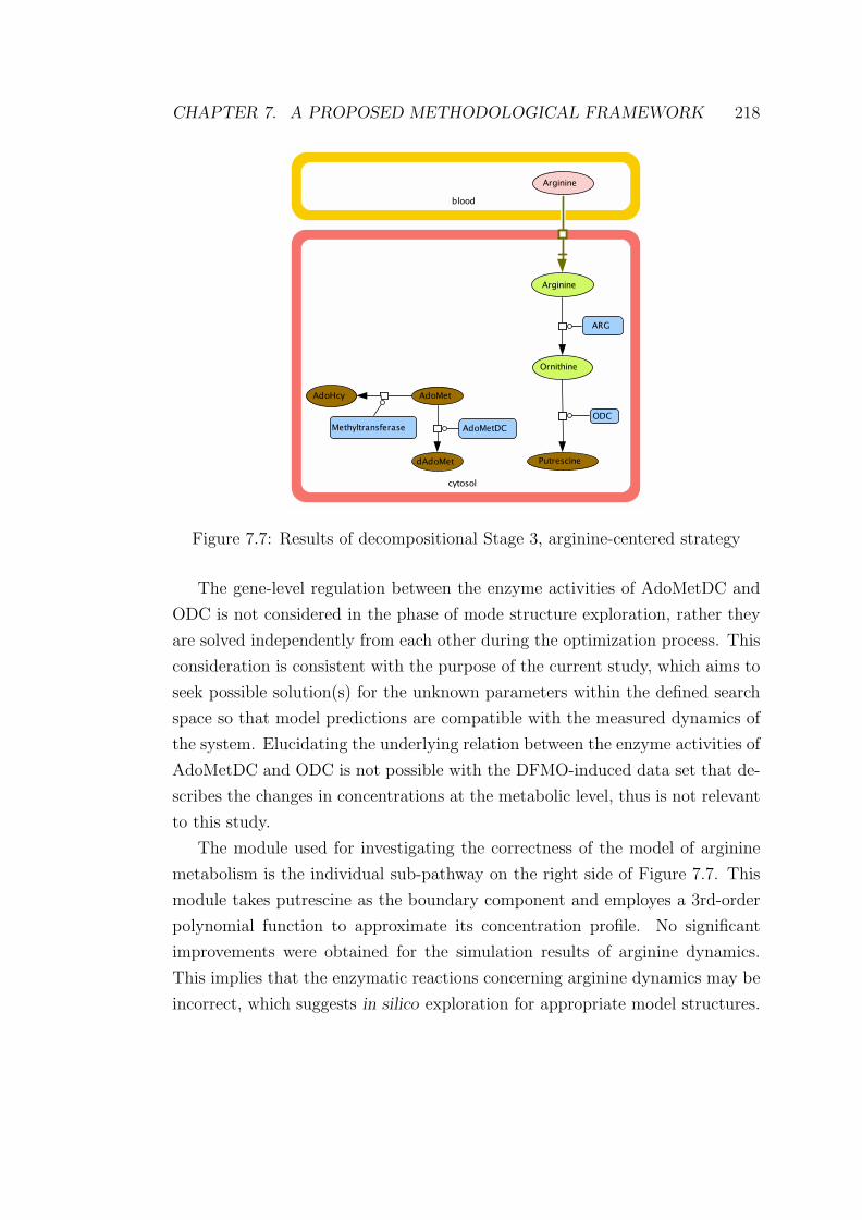
Appendix B
Structural Analysis
B.1 The Computational Approach for Detect-
ing Network Gaps
The main idea of the computational investigation is to examine, after adding
new branches to one metabolite at a time, whether the elementary modes of
the new topology can cover all the enzymatic reactions. Elementary modes are
computed with the package METATOOL, where the stoichiometric matrix is
used as a direct input.
With the assumption that additional reactions occur in isolation, the num-
ber of structural topologies to be examined is equal to the number of internal
metabolites. Computationally, additional reactions are embodied in the last col-
umn of the original stoichiometric matrix, where a non-zero entry in the column
represents the involvement of the metabolite in the corresponding reaction.
By way of example, let’s assume that the internal metabolite arginine has an
additional outgoing branch. Accordingly, the original matrix is expanded with
an additional column. There are no changes to the rows as no new metabolites
are included. The last column of the expanded matrix is given by the following
vector [−1 0 0 0 0 0 0 0 0 0 0 0 0 0 0 0 0 0
]where the non-zero entry ‘-1’ represents the consumption of arginine in the
additional reaction. As we assume that the additional reactions take place in
isolation–one reaction at a time, there is only one non-zero entry in the vector.
We also examined the structural topology when the additional reactions of
the internal metabolites are assumed to take place in pairs. In this case, two ad-
272

APPENDIX B. STRUCTURAL ANALYSIS 273
ditional branches are appended to the end of the original stoichiometric matrix
(Stb). The number of scenarios to be examined for network gaps is the number
of possible combinations for the selection of 2 metabolites from n pairs, which isn!
k!·(n−k)!, where n! denotes the factorial of n, the number of internal metabolites
and k is the number of components selected (i.e. 2). When selecting any two
from 18 internal metabolites, there are 153 possible pairings to examine. Com-
putational results of this examination are detailed in the section ‘Network Gaps
Identification’ in Chapter 3.
B.2 Mass-balance Model of the Trypanothione
Pathway in ST1
This section presents the mass-balance model and the stoichiometric matrix of
the trypanothione metabolic pathway represented by structural topology ST1.
Refer to texts in Section 3.4 for a detailed description. Structural topology
ST1 introduced a new reaction concerning trypanothione consumption in other
metabolic functions to Table 3.1, written as
No. Label Reaction Name Stochiometry22 υtshout TSH Consumption TSH → tsh end

APPENDIX B. STRUCTURAL ANALYSIS 274
X1 = d[Arg]dt = 0 = barg − υ1
X2 = d[Orn]dt = 0 = υ1 − υ2
X3 = d[Met]dt = 0 = bmet − υ3 + υ7
X4 = d[AdoMet]dt = 0 = υ3 − υ4 − υ5
X5 = d[Put]dt = 0 = υ2 − υ6
X6 = d[dAdoMet]dt = 0 = υ4 − υ6
X7 = d[Spd]dt = 0 = υ6 − υ10 + υ11
X8 = d[MTA]dt = 0 = υ6 − υ7
X9 = d[Cys]dt = 0 = bcys − befcys + υ5 − υ8
X10 = d[Glu]dt = 0 = bglu − υ8
X11 = d[Gly]dt = 0 = bgly − υ9
X12 = d[gGluCys]dt = 0 = υ8 − υ9
X13 = d[GSH]dt = 0 = υ9 − 2 · υ10 + 2 · υ11
X14 = d[TSH]dt = 0 = υ10 − υ11 − υ12 + υ13 − υtshout
X15 = d[TS2]dt = 0 = υ12 − υ13
X16 = d[G6P ]dt = 0 = bglc − υ14
X17 = d[NADPH]dt = 0 = −υ13 + υ14
X18 = d[NADP ]dt = 0 = υ13 − υ14
(B.1)
[d[Arg]dt
d[Orn]dt
d[Met]dt
d[AdoMet]dt
d[Put]dt
d[dAdoMet]dt
d[Spd]dt
d[MTA]dt
d[Cys]dt
d[Glu]dt
d[Gly]dt
d[gGluCys]dt
d[GSH]dt
d[TSH]dt
d[TS2]dt
d[G6P ]dt
d[NADPH]dt
d[NADP ]dt ]T =
Stb · [υ1 υ2 υ3 υ4 υ5 υ6 υ7 υ8 υ9 υ10 υ11 υ12 υ13 υ14
barg bmet bcys beff bglu bgly bglc υtshout]T
where
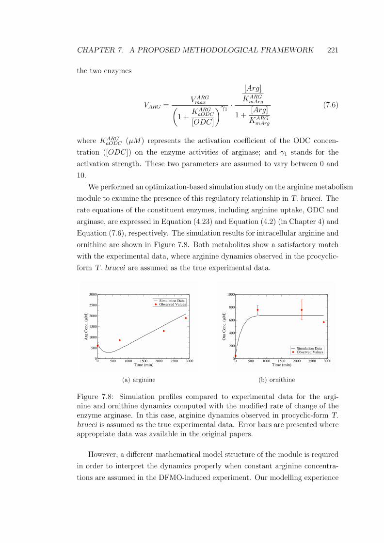
APPENDIX B. STRUCTURAL ANALYSIS 275
Stb =
2666666666666666666666666666664
−1 0 0 0 0 0 0 0 0 0 0 0 0 0 1 0 0 0 0 0 0 01 −1 0 0 0 0 0 0 0 0 0 0 0 0 0 0 0 0 0 0 0 00 0 −1 0 0 0 1 0 0 0 0 0 0 0 0 1 0 0 0 0 0 00 0 1 −1 −1 0 0 0 0 0 0 0 0 0 0 0 0 0 0 0 0 00 1 0 0 0 −1 0 0 0 0 0 0 0 0 0 0 0 0 0 0 0 00 0 0 1 0 −1 0 0 0 0 0 0 0 0 0 0 0 0 0 0 0 00 0 0 0 0 1 0 0 0 −1 1 0 0 0 0 0 0 0 0 0 0 00 0 0 0 0 1 −1 0 0 0 0 0 0 0 0 0 0 0 0 0 0 00 0 0 0 1 0 0 −1 0 0 0 0 0 0 0 0 1 −1 0 0 0 00 0 0 0 0 0 0 −1 0 0 0 0 0 0 0 0 0 0 1 0 0 00 0 0 0 0 0 0 0 −1 0 0 0 0 0 0 0 0 0 0 1 0 00 0 0 0 0 0 0 1 −1 0 0 0 0 0 0 0 0 0 0 0 0 00 0 0 0 0 0 0 0 1 −2 2 0 0 0 0 0 0 0 0 0 0 00 0 0 0 0 0 0 0 0 1 −1 −1 1 0 0 0 0 0 0 0 0 −10 0 0 0 0 0 0 0 0 0 0 1 −1 0 0 0 0 0 0 0 0 00 0 0 0 0 0 0 0 0 0 0 0 0 −1 0 0 0 0 0 0 1 00 0 0 0 0 0 0 0 0 0 0 0 −1 1 0 0 0 0 0 0 0 00 0 0 0 0 0 0 0 0 0 0 0 1 −1 0 0 0 0 0 0 0 0
3777777777777777777777777777775
(B.2)
B.3 LP Optimization for Maximum Growth Rate
When the mass-balance model in Equation (B.1) is used for the maximization of
growth yield, the reaction labelled as υtshout is replaced with the growth rate υgr.
The stoichiometric matrix formulated in (B.2) is used for the task of interest.
From the biological point of view, the last column in this matrix represents the
reaction flux converting the metabolite precursor into biomass components.
B.4 LP Optimization for Minimum Residual Er-
ror with Respect to H2O2 Production Rate
The following mass-balance model is employed for the prediction of gene essen-
tiality, expressing the residual error between the calculated and measured rate of
H2O2 production as an objective. The optimal steady-state fluxes of individual
reactions are calculated by minimizing the error.
The mass-balance model for LP optimization of the minimum residual er-
ror below is based on Equation (B.1) given in Appendix B.2. To enable the
H2O2 production rate to be computationally simulated, H2O2 is considered as
a variable metabolite and the corresponding mass-balance equation is formu-
lated, which is specified by X16. This introduces a new reaction flux to the
mass-balance model in Equation (B.1), written as below

APPENDIX B. STRUCTURAL ANALYSIS 276
No. Label Reaction Name Stochiometry23 rH2O2 H2O2 production H2O2 Source → H2O2
X1 = d[Arg]dt = 0 = barg − υ1
X2 = d[Orn]dt = 0 = υ1 − υ2
X3 = d[Met]dt = 0 = bmet − υ3 + υ7
X4 = d[AdoMet]dt = 0 = υ3 − υ4 − υ5
X5 = d[Put]dt = 0 = υ2 − υ6
X6 = d[dAdoMet]dt = 0 = υ4 − υ6
X7 = d[Spd]dt = 0 = υ6 − υ10 + υ11
X8 = d[MTA]dt = 0 = υ6 − υ7
X9 = d[Cys]dt = 0 = bcys − befcys + υ5 − υ8
X10 = d[Glu]dt = 0 = bglu − υ8
X11 = d[Gly]dt = 0 = bgly − υ9
X12 = d[gGluCys]dt = 0 = υ8 − υ9
X13 = d[GSH]dt = 0 = υ9 − 2 · υ10 + 2 · υ11
X14 = d[TSH]dt = 0 = υ10 − υ11 − υ12 + υ13 − υtshout
X15 = d[TS2]dt = 0 = υ12 − υ13
X16 = d[G6P ]dt = 0 = bglc − υ14
X17 = d[NADPH]dt = 0 = −υ13 + υ14
X18 = d[NADP ]dt = 0 = υ13 − υ14
X19 = d[H2O2]dt = 0 = rH2O2 − υ12
(B.3)

Appendix C
System Identifiability
In this appendix we detail the mathematical concepts behind the computational
procedures developed for identifiability analysis, including the details for the
numerical computation of Jacobian matrix, Fisher information matrix, covari-
ance and correlation matrices, confidence intervals and other related statistical
measures.
C.1 A Priori Structural Identifiability
Structural identifiability analysis is performed to investigate whether all model
parameters can be estimated given the available knowledge of the system. Out-
put sensitivity functions are central to the evaluation of a priori local identifiabil-
ity. Linearly dependent sensitivity functions result in parameter estimates that
are correlated. In our study, the numerical method for checking local structural
identifiability is based on the description given by Zak et al. (Zak et al. 2003).
Suppose the system is expressed as a set of Nx differential equations with Nx
states (x) and Np parameters (p). Taking p as ‘true values’ of the parameter
set, the Nx × Np sensitivity matrices of the measured states are calculated at a
large enough number of points N where:
Sx(i,j) =
(∂xi
∂pj
)x=x(t,p), p=p
The correlation matrix of the parameters (Mc) was calculated:
Mc = correlation(G)
277

APPENDIX C. SYSTEM IDENTIFIABILITY 278
where
G =
⎡⎢⎢⎢⎢⎣
Sx(t1)
Sx(t2)...
Sx(tN)
⎤⎥⎥⎥⎥⎦
Parameters that are locally identifiable have correlations with all other pa-
rameters between -1 and +1. Parameters that are not locally identifiable have
correlations of exactly -1 or +1 with at least one other parameter.
Sensitivity matrices Sxij have to be calculated for the measured states at a
large number of time points to diminish the numerical bias introduced from the
lack of points.
Computing the sensitivity matrix involves calculating the gradient of each
component of the gradient vector of the system output. One possibility is to
evaluate these gradients using finite differences: perturbing each independent
parameter p in turn, calculating the perturbed gradient of each system state
x, subtracting the unperturbed gradient, and dividing by the magnitude of the
perturbation (Dennis and Schnabel 1983).
The method of finite difference approximation is straightforward in that only
the calculation of xi is required with nominal and perturbed parameters. How-
ever, the numerical values obtained may vary significantly with Δθj, and re-
peated solutions of the model are required for each parameter. The central
finite difference is used in the computation of sensitivity matrix with the form
below. This method, compared with the forward and backward finite difference
approximation, gives rise to the smallest round-off error.
si,j(t) =∂xi(t)
∂θi
=xi(θj + Δθj, t) − xi(θj − Δθj, t)
2 ∗ Δθj
(C.1)
C.2 Practical Identifiability with Hessian Ma-
trix
A unified formalism for constructing the Hessian matrix is given in this section.
A Hessian matrix is the second derivative of the objective function G with
respect to the parameters. Let Δ = (Δθ1, . . . , Δθi) be the estimates of Δθ, and
G = (G1, . . . , Gj) be the objective function values calculated for each of system
APPENDIX C. SYSTEM IDENTIFIABILITY 279
states. The Hessian matrix is defined as follows⎛⎜⎜⎜⎜⎜⎜⎜⎜⎜⎜⎜⎜⎝
∂G1
∂θ1
∂G2
∂θ1. . .
∂Gj
∂θ1
∂G1
∂θ2
∂G2
∂θ2. . .
∂Gj
∂θ2
......
. . ....
∂Gj
∂θi
∂Gj
∂θi. . .
∂Gj
∂θi
⎞⎟⎟⎟⎟⎟⎟⎟⎟⎟⎟⎟⎟⎠
To investigate the practical identifiability, a Hessian matrix (Hij) of partial
derivatives of the objective function with respect to the parameter vector has to
be formulated.
Hij = (JTJ)ij +n∑
i=1
rl · ∂2Gij
∂θi∂θj
where J is the Jacobian or gradient matrix of the objective function with respect
to the parameter vector in the form of
Jij =∂Gij(θ)
∂θj
(C.2)
In the presence of small residuals, the Gauss-Newton approximation to the
Hessian states that the terms containing the residuals can be ignored, thus giving
the following equation:
Hij = (JTJ)ij (C.3)
The Jacobian matrix J records the absolute difference between the objective
function calculated with the nominal value of θj in the parameter vector θ and
the perturbed value, which can be computed with the central finite difference in
Equation (C.1).
The Hessian matrix is often called the Fisher information matrix. Inverting
the Hessian matrix gives the approximate Variance-Covariance matrix as follow
Mvc =
⎛⎜⎜⎜⎜⎝
σ2i=1,i=1 σi=1,i=2 . . . σi=1,i=i
σi=2,i=1 σ2i=2,i=2 . . . σi=2,i=i
......
. . ....
σi=i,i=1 σi=i,i=2 . . . σ2i=i,i=i
⎞⎟⎟⎟⎟⎠ (C.4)
The diagonal elements of the Variance-Covariance matrix are the variances,
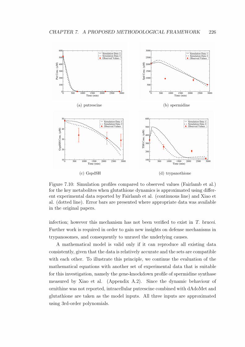
APPENDIX C. SYSTEM IDENTIFIABILITY 280
which can be used to construct confidence intervals for the parameters. The
correlation coefficients between parameters pi and the pj are approximated by:
Rpi,pj=
Cpi,pj√Cpi,piCpj,pj
, pi �= pj
Rpi,pj= 1, pi = pj
The correlation matrix measures the relationship between the parameters
and indicates pairs of parameters where changes in the model output due to a
change in one parameter value can be compensated by an appropriate change in
an other parameter value.
With the Variance-Covariance matrix, 95% confidence intervals can be cal-
culated for any identifiable parameters, which are given as:
CI = pi ± 1.96σ(pi)
where pi denotes the nominal parameter value. Here, symmetry of the confidence
region about the nominal values is assumed.

Bibliography
Albert, M.-A., Haanstra, J. R., Hannaert, V., Roy, J. V., Opperdoes, F. R.,
Bakker, B. M. and Michels, P. A. M.: 2005, Experimental and in Silico
analyses of glycolytic flux control in bloodstream form Trypanosoma brucei,
The Journal of Biological Chemistry 280(31), 28306–28315.
Alhonen-Hongisto, L., Seppanen, P. and Janne, J.: 1980, Intracellular pu-
trescine and spermidine deprivation induces increased uptake of the na-
trual polyamines and methylglyoxal bis(guanylhydrazone), The Journal of
Biological Chemistry 192, 941–945.
Anderson, D. R., Burnham, K. P. and Thompson, W. L.: 2000, Null hypoth-
esis testing: problems, prevalence and an alternative, Journal of Wildlife
Management 64, 912–923.
Ariyanayagam, M. R. and Fairlamb, A. H.: 2001, Ovothiol and trypanothione
as antioxidants in trypanosomatids, Molecular & Biochemical Parasitology
115, 189–198.
Ascher, U. M., Matthejj, R. and Russell, R.: 1995, Numerical Solution of Bound-
ary Value Problems for Ordinary Differential Equations, SIAM, Philadel-
phia.
Ascher, U. M. and Petzold, L. R.: 1998, Computer methods for ordinary differ-
ential equations and differential-algebraic equations, SIAM.
Asthagiri, A. R. and Lauffenburger, D. A.: 2001, A computational study of
feedback effects on signal dynamics in a mitogen-activated protein kinase
(mapk) pathway model, Biotechnol. Prog. 17, 227–239.
Audet, C. and Dennis, J. E.: 2000, Analysis of generalized pattern searches,
SIAM J. Optim 13, 889–903.
281

BIBLIOGRAPHY 282
Bacchi, C. J., Garofalo, J., Mockenhaupt, D., McCann, P. P., Diekema, K. A.,
Pegg, A. E., Nathan, H. C., Mullaney, E. A., Chunosoff, L., Sjoerdsma, A.
and Hutner, S. H.: 1983, In vivo effects of α-DL-difluoromethylornithine on
the metabolism and morphology of Trypanosoma brucei brucei, Molecular
and Biochemical Parasitology 7, 209–225.
Bacchi, C. J., Goldberg, B., Garofalo-Hannan, J., Rattendi, D., Lyte, P. and
Yarlett, N.: 1995, Fate of soluble methionine in African trypanosomes:
effects of metabolic inhibitors, Biochemistry 309, 737–743.
Bacchi, C. J., Lipschik, G. Y. and Nathan, H. C.: 1977, Polyamines in Try-
panosomatids, Journal of Bacteriology 131(2), 657–661.
Bacchi, C. J., Nathan, H. C., Hutner, S. H., McCann, P. P. and Sjoerdsma,
A.: 1980, Polyamine metabolism: A potential therapeutic target in Try-
panosomes, Science 210, 332–334.
Bacchi, C. J., Sufrin, J. R., Nathan, H. C., Spoess, A. J., Hannan, T., Garo-
falo, J., Alecia, K., Katz, L. and Yarlett, N.: 1991, 5’-Alkyl-substituted
analogs of 5’-Methylthioadenosine as Trypanocides, Antimicrobial Agents
and Chemotherapy 35(7), 1315–1320.
Bacchi, C. J. and Yarlett, N.: 2002, Polyamine metabolism as chemotherapeutic
target in protozoan parasites, Mini Reviews in Medicinal Chemistry 2, 553–
563.
Bailey, J. E.: 1998, Mathematical modeling and analysis in biochemical en-
gineering: Past accomplishments and future opportunities, Biotechnology
Progress 14(1), 8–20.
Bakker, B. M.: 1998, Control and regulation of glycolysis in Trypanosoma brucei,
PhD thesis, Vrije Universiteit.
Bakker, B. M., Assmus, H. E., Bruggeman, F., Haanstra, J. R., Klipp, E. and
Westerhoff, H.: 2002, Network-based selectivity of antiparasitic inhibitors,
Molecular Biology Reports 29, 1–5.
Bakker, B. M., Michels, P. A. M., Opperdoes, F. R. and Westerhoff, H. V.: 1997,
Glycolysis in bloodstream form Trypanosoma brucei can be understood in
terms of the kinetics of the glycolytic enzymes, The Journal of Biological
Chemistry 272(6), 3207–3215.

BIBLIOGRAPHY 283
Baldi, P. and Hatfield, G. W.: 2002, DNA Microarrays and Gene Expression,
Cambridge University Press, chapter Chapter 8. Systems Biology, pp. 135–
165.
Barrett, M. P.: 1997, The pentose phosphate pathway and parasitic protozoa,
Parasitology Today 13(1), 11–16.
Barrett, M. P., Burchmore, R. J., Stich, A., Lazzari, J. O., Frasch, A. C.,
Cazzulo, J. J. and Krishna, S.: 2003, The trypanosomiases, The Lancet
362, 1469–1480.
Basselin, M., Lawrence, F. and Robert-Gero, M.: 1996, Pentamidine uptake in
leishmania donovani and leishmania amazonensis promastigotes and axenic
amastigotes, Biochemistry 315, 631–634.
Behre, J., Wilhelm, T., von Kamp, A., Ruppin, E. and Schuster, S.: 2008, Struc-
tural robustness of metabolic networks with respect to multiple knockouts,
Journal of Theoretical Biology 252, 433–441.
Bellofatto, V., Fairlamb, A. H., Henderson, G. B. and Cross, G. A. M.: 1987,
Biochemical changes associated with α-difluoromethylornithine uptake and
resistance in trypanosoma brucei, Molecular and Biochemical Parasitology
25, 227–238.
Bentele, M., Lavrik, I., Ulrich, M., Stoβer, S., Heermann, D. W., Kalthoff,
H., Krammer, P. H. and Eils, R.: 2004, Mathematical modeling reveals
threshold mechanism in cd95-induced apoptosis, The Journal of Cell Biol-
ogy 166(6), 839–851.
Berg, J. M., Tymoczko, J. L., Stryer, L. and Clarke, N. D.: 2002, Biochemistry,
W. H. Freeman and Company, chapter 15. Signal-transduction pathways:
An introduction to information metabolism.
Berger, B. J., Dai, W. W., Wang, H., Stark, R. E. and Cerami, A.: 1996, Aro-
matic amino acid transamination and methionine recycling in trypanoso-
matids, Proc. Natl. Acad. Sci. 93, 4126–4130.
Beswick, T. C., Willert, E. K. and Phillips, M. A.: 2006, Mechanisms of allosteric
regulation of trypanosoma cruzi S-Adenosylmethionine decarboxylase, Bio-
chemistry 45, 7797–7807.

BIBLIOGRAPHY 284
Birnbaumer, L., Bearer, C. F. and Iyengar, R.: 1980, A two-state model of
an enzyme with an allosteric regulatory site capable of metabolizing the
regulatory ligand, The Journal of Biological Chemistry 255(8), 3552–3557.
Bitonti, A. J., Bacchi, C. J., McCann, P. P. and Sjoerdsma, A.: 1985, Cat-
alytic irreversible inhibition of Trypanosoma brucei brucei ornithine de-
carboxylase by substrate and product analogs and their effects on murine
trypanosomiasis, Biochem Pharmacol 34(10), 1773–1777.
Bitonti, A. J., Dumont, J. A. and McCann, P. P.: 1986, Characterization of
trypanosoma brucei brucei S-adenosyl-L-methione decarboxylase and its in-
hibition by Berenil, pentamidine and methylglyoxal bis(guanylhydrazone),
The Journal of Biological Chemistry 237, 685–689.
Bitonti, A. J., Kelly, S. E. and McCann, P. P.: 1984, Characterization of spermi-
dine synthase from trypanosoma brucei brucei, Molecular and Biochemical
Parasitology 13, 21–28.
Blasius, B., Beck, F. and Luttge, U.: 1998, Oscillatory model of Crassulacean
acid metabolism: structural analysis and stability boundaries with a dis-
crete hysteresis switch, Plant Cell Environ 21, 775–784.
Bock, H. G.: 1982, Recent advances in parameter estimation identification tech-
niques for ode, in P. Deuflhard and E. Hairer (eds), Numerical treatment of
inverse problems in differential and integral equations, pp. 95–112.
Bollinger, J. M., Kwon, J. D. S., Huisman, G. W., Kolter, R. and Walsh, C. T.:
1995, Glutathionylspermidine metabolism in escherichia coli, The Journal
of Biological Chemistry 270(23), 14031–14041.
Bower, J. M. and Bolouri, H.: 2001, Computational Modelling of Genetic and
Biochemical Networks, MIT Press.
Box, G. E. P.: 1979, Robustness in the strategy of scientific model building, in
R. L. Launer and G. N. Wilkinson (eds), Robustness in Statistics, Academic
Press Inc.,U.S., pp. 201–236.
Box, G. E. P. and Hill, W. J.: 1967, Discriminating among mechanistic models,
Technometrics 9(1), 57–71.

BIBLIOGRAPHY 285
Breitling, R., Vitkup, D. and Barrett, M. P.: 2008, New surveyor tools for
charting microbial metabolic maps, Nature 6, 156–161.
Burgard, A. P. and Maranas, C. D.: 2003, Optimization-based framework for
inferring and testing hypothesized metabolic objective functions, Biotech-
nology and Bioengineering 82(6), 670–677.
Calder, M., Gilmore, S. and Hillston, J.: 2006, Modelling the influence of rkip
on the erk signalling pathway using the stochastic process algebra pepa,
Lecture Notes in Computer Science 4230, 1–23.
Cascante, M., Boros, L. G., Comin-Anduix, B., de Atauri, P., Centelles, J. J.
and Lee, P. W.-N.: 2002, Metabolic control analysis in drug discovery and
disease, Nature Biotechnology 20, 243–249.
Cederbaum, S. D., Yu, H., Grody, W. W., Kern, R. M., Yoo, P. and Iyer, R. K.:
2003, Arginases i and ii: do their functions overlap?, Molecular Genetics
and Metabolism 81(1), 38–44.
Chavali, A. K., Whittemore, J. D., Eddy, J. A., Williams, K. T. and Papin, J. A.:
2008, Systems analysis of metabolism in the pathogenic trypanosomatid
Leishmaina major, Molecular Systems Biology 4(177), 1–19.
Chiang, P. K., Gordon, R. K., Tal, H., Zeng, G. C., Doctor, B. P., Pardhasaradhi,
K. and McCann, P. P.: 1996, S-Adenosylmethionine and methylation, The
FASEB Journal 10, 471–480.
Childs, B. and Osborne, M.: 1996, Fitting solutions of ordinary differential
equations to observed data, in R. L. May and A. K. Easton (eds), Compu-
tational techniques and applications: CTAC’95, World Scientifc Publishing
Co, Singapore, pp. 193–198.
Cho, K.-H., Shin, S.-Y., Kim, H.-W., Wolkenhauer, O., McFerran, B. and Kolch,
W.: 2003, Mathematical modeling of the influence of RKIP on the ERK sig-
naling pathway, in C. Priami (ed.), Conference of Computational Methods
in Systems Biology (CSMB’03), Vol. 2602, Springer-Verlag, pp. 127–141.
Cho, K.-H. and Wolkenhauer, O.: 2003, Analysis and modelling of signal trans-
duction pathways in systems biology, Biochemical Society Transactions
31, 1503–1509.

BIBLIOGRAPHY 286
Christa, L., Kersual, J., Auge, J. and Perignon, J.-L.: 1988, Methylthioadeno-
sine toxicity and metabolism to methionine in mammalian cells, Journal of
Biochemistry 255, 145–152.
Coello, C. A. C.: 2001, A short tutorial on evolutionary multiobjective opti-
mization, Proceedings of the First International Conference on Evolutionary
Multi-Criterion Optimization, Springer-Verlag, pp. 21–40.
Coello, C. A. C.: 2002, Theoretical and numerical constraint-handling tech-
niques used with evolutionary algorithms: a survey of the state of the art,
Computer Methods in Applied Mechanics and Engineering 191, 1254–1287.
Coello, C. A. C. and Lechuga, M. S.: 2002, Mopso: a proposal for multiple
objective particle swarm optimization, In Proceedings of the 2002 Congess
on Evolutionary Computation, part of the 2002 IEEE World Congress on
Computational Intelligence, IEEE Press, Hawaii, pp. 1051–1056.
Coello, C. A. C., Pulido, G. T. and Lechuga, M. S.: 2004, Handling multiple
objectives with particle swarm optimization, IEEE Transactions on evolu-
tionary computation 8(3), 256–279.
Comini, M. A., Guerrero, S. A., Haile, S., Menge, U., Lunsdorf, H. and Flohe,
L.: 2004, Validation of Trypanosoma brucei trypanothione synthetase as
drug target, Free Radical Biology & Medicine 36(10), 1289–1302.
Cook, P. F. and Cleland, W. W.: 2007, Enzyme Kinetics and Mechanism, Gar-
land Science, New York, USA.
Covert, M. W., Xiao, N., Chen, T. J. and Karr, J. R.: 2008, Integrating
metabolic, transcriptional regulatory and signal transduction models in Es-
cherichia coli, Bioinformatics 24(8), 2044–2050.
Crampin, E. J.: 2006, System identification challenges from systems biology, 14th
IFAC Symposium on System Identification, Newcastle, Australia, pp. 81–93.
Crampin, E. J., McSharry, P. E. and Schnell, S.: 2004, Extracting biochem-
ical reaction kinetics from time series data, Knowledge-Based Intelligent
Information and Engineering Systems, Pt 2, Proceedings 3214, 329–336.

BIBLIOGRAPHY 287
Crampin, E. J., Schnell, S. and McSharry, P. E.: 2004, Mathematical and com-
putational techniques to deduce complex biochemical reaction mechanism,
Progress in Biophysics & Molecular Biology 86, 77–112.
Cronin, C. N., Nolan, D. P. and Voorheis, H. P.: 1989, The enzymes of the clas-
sical pentose phosphate pathway display differential activities in procyclic
and bloodstreams forms of Trypanosome brucei, FEBS Letters 244(1), 26–
30.
da Fonseca, C. M. M.: 1995, Multiobjective genetic algorithms with application
to control engineering problems, PhD thesis, University of Sheffield.
Darlyuk, L., Goldman, A., Roberts, S. C., Ullman, B., Rentsch, D. and Zilber-
stein, D.: 2009, Arginine homeostasis and transport in the human pathogen
Leishmania donovani, Journal of Biology Chemistry 284(30), 19800–19807.
de Jong, H.: 2002, Modeling and simulation of genetic regulatory systems: A
literature review, Computational Biology 9(1), 67–103.
Deb, K., Agrawal, S., Pratap, A. and Meyarivan, T.: 2000, A fast elitist
non-dominated sorting genetic algorithm for multi-objective optimization:
Nsga-ii, Proceedings of the 6th International Conference on Parallel Prob-
lem Solving from Nature, Springer, pp. 849–858.
Dennis, J. E. and Schnabel, R. B.: 1983, Numerical methods for unconstrained
optimization and nonlinear equations, Prentice-Hall, Englewood Cliffs.
Duarte, N. C., Herrgard, M. J. and ∅ Palsson, B.: 2004, Reconstruction and
validation of Saccharomyces cerevisiae ind750, a fully compartmentalized
genome-scale metabolic model, Genome Research 14, 1298–1309.
Duffieux, F., Roy, J. V., Michels, P. A. M. and Opperdoes, F. R.: 2000, Molec-
ular characterization of the first two enzymes of the pentose-phosphate
pathway of Trypanosoma brucei, The Journal of Biological Chemistry
275(36), 27559–27565.
Duszenko, M., Ferguson, M. A. J., Lamont, G. S., Rifkin, M. R. and Cross, G.
A. M.: 1985, Cysteine eliminates the feeder cell requirement for cultivation
of trypanosoma brucei, The Journal of Experimental Medicine 162, 1256–
1263.

BIBLIOGRAPHY 288
Eberhart, R. C. and Shi, Y.: 1998, Comparison between genetic algorithms and
particle swarm optimization, The 7th Annual Conference on Evolutionary
Programming, San Diego, USA.
Edwards, J. S. and Palsson, B. O.: 2000a, Metabolic flux balance analysis and
the in silico analysis of Escherichia coli k-12 gene deletions, BMC Bioinfor-
matics 1(1), 1–10.
Edwards, J. S. and Palsson, B. O.: 2000b, The Escherichia coli MG1655 in silico
metabolic genotype: its definition, characteristics, and capabilities, PNAS
97(10), 5528–5533.
Eisenthal, R. and Cornish-Bowden, A.: 1998, Prospects for antiparasitic drugs,
The Journal of Biological Chemistry 273(10), 5500–5505.
Endy, D. and Brent, R.: 2001, Modelling cellular behaviour, Nature 409, 391–
395.
Erdi, P. and Toth, J.: 1988, Mathematical models of chemical reactions: theory
and applications of deterministic and stochastic models (Nonlinear science),
Manchester University Press.
Fairlamb, A. H.: 2003, Chemotherapy of human African trypanosomiasis: cur-
rent and future prospects, Trends in Parasitology 19(11), 488–494.
Fairlamb, A. H., Blackburn, P., Ulrich, P., Chait, B. T. and Creami, A.: 1985,
Trypanothione: A Novel Bio(glutathionyl)spermidine Cofactor for Glu-
tathione Reductase in Trypanosomatids, Science 227, 1485–1487.
Fairlamb, A. H., Henderson, G. B., Bacchi, C. J. and Cerami, A.: 1987, In vivo
effects of difluoromethylornithine on trypanothione and polyamine levels
in bloodstream forms of Trypanosoma brucei, Molecular and Biochemical
Parasitology 24, 185–191.
Faller, D., Klingmuller, U. and Timmer, J.: 2003, Simulation methods for opti-
mal experimental design in Systems Biology, SIMULATION 79, 717–725.
Fell, D. A.: 1997, Systems properties of metabolic networks, in Y. Bar-Yam (ed.),
Proceedings of the International Conference on Complex Systems, Nashua,
NH, pp. 21–26.

BIBLIOGRAPHY 289
Fieldsend, J. E.: 2004, Multi-objective particle swarm optimization methods,
Technical report, Department of Computer Science, University of Exeter.
Fieldsend, J. E. and Singh, S.: 2002, A multi-objective algorithm based upon
particle swarm optimization, an efficient data structure and turbulence,
In Proceedings of UK Workshop on Computational Intelligence (UKCI’02),
Birmingham, UK, pp. 37–44.
Fisher, J. and Henzinger, T. A.: 2008, Executable cell biology, Nature Biotech-
nology 25, 1239–1249.
Fonseca, C. M. and Fleming, P. J.: 1993, Genetic algorithms for multiobjective
optimization: Formulation, discussion and generalization, Genetic Algo-
rithms: Proceedings of the Fifth International Conference, Morgan Kauf-
mann, pp. 416–423.
Fonseca, C. M. and Fleming, P. J.: 1995, An overview of evolutionary algorithms
in multiobjective optimization, Evolutionary Computation 3, 1–16.
Fouce, R. B., Escribano, M. I. and Alunda, J. M.: 1991, Putrescine uptake regu-
lation in response to alpha-difluoromethylornithine treatment in leishmania
infantum promastigotes, Molecular and Cellular Biochemistry 107, 127–
133.
Fyfe, P. K., Oza, S. L., Fairlamb, A. H. and Hunter, W. N.: 2008, Leishmania
trypanothione synthetase-amidase structure reveals a basis for regulation of
conflicting synthetic and hydrolytic activities, Journal of Biological Chem-
istry 283, 17672–17680.
Gardner, T. S., di Bernardo, D., Lorenz, D. and Collins, J. J.: 2003, Inferring
genetic networks and identifying compound mode of action via expression
profiling, Science 301, 102–105.
Garfinkel, D.: 1971, Resolution by computer simulation of contradictory exper-
imental findings as to the effect on gluconeogenesis of oleate addition in
perfused rat liver, Biochemical and Biophysical Research Communications
42(4), 621–626.
Ge, H.-W., Liang, Y.-C. and Marchese, M.: 2007, An improved particle swarm
optimization-based dynamic recurrent neural network for identifying and

BIBLIOGRAPHY 290
controlling nonlinear systems, Computers and Structures 85(21-22), 1611–
1622.
Geier, F., Timmer, J. and Fleck, C.: 2007, Reconstructing gene-regulatory net-
works from time series, knock-out data and prior knowledge, BMC Systems
Biology 1(11), 1–16.
Ghoda, L., Sidney, D., Macrae, M. and Coffino, P.: 1992, Structural el-
ements of ornithine decarboxylase required for intracellular degrada-
tion and polyamine-dependent regulation, Molecular and Cellular Biology
12(5), 2178–2185.
Ghoda, L. Y., Phillips, M. A., Bass, K. E., Wang, C. C. and Coffino, P.:
1990, Trypanosome ornthine decarboxylase is stable because it lacks se-
quences found in carboxyl terminus of the mouse enzyme which target the
latter for intracellular degradation, The Journal of Biological Chemistry
265(20), 11823–11826.
Ghoda, L. Y., Savarese, T. M., Northrup, C. H., R. E. Parks, J., Garofalo, J.,
Katz, L., Ellenbogen, B. B. and Bacchi, C. J.: 1988, Substrate specifici-
ties of 5’-deoxy-5’-methylthioadenosine phosphorylase from Trypanosoma
brucei brucei and mammalian cells, Mol. Biochem. Parasitol. 27, 109–118.
Gilbert, D., Fuβ, H., Gu, X., Orton, R., Robinson, S., Vyshemirsky, V., Kurth,
M. J., Downes, C. S. and Dubitzky, W.: 2006, Computational methodolo-
gies for modelling, analysis and simulation of signalling networks, Briefings
in Bioinformatics 7(4), 339–353.
Gillespie, D. T.: 1977, Exact stochastic simulation of coupled chemical reactions,
J. Phys. Chem 81(25), 2340–2361.
Girolami, M.: 2008, Bayesian inference for differential equations, Theoretical
Computer Science 408(1), 4–16.
Girvan, M. and Newman, M. E. J.: 2001, Community structure in social and
biological networks, PNAS 99(12), 7821–7826.
Gobert, A. P., Daulouede, S., Lepoivre, M., Boucher, J. L., Bouteille, B., Buguet,
A., Cespuglio, R., Veyret, B. and Vincendeau, P.: 2000, L-arginine avail-
ability modulates local nitric oxide production and parasitic killing in ex-
perimental trypanosomiasis, Infection and Immunity 68(8), 4653–4657.

BIBLIOGRAPHY 291
Goldberg, B., Rottendi, D., Lloyd, D., Yarlett, N. and Bacchi, C. J.: 2000,
Kinetics of methionine transport and metabolism by trypanosoma brucei
brucei and trypanosoma brucei rhodesiense, Archives of Biochemistry and
Biophysics 377(1), 49–57.
Goldberg, D. E.: 1989, Genetic Algorithms in Search, Optimization and Machine
Learning, Addison-Wesley Publishing Company, Reading, Massachusetts.
Golub, G., Klema, V. and Stewart, G. W.: 1976, Rank degeneracy and least
squares problems, Technical Report TR-456, Department of Computer Sci-
ence, University of Maryland, College Park, MD.
Grosan, C., Abraham, A., Han, S. and Gelbukh, A.: 2005, Hybrid particle
swarm - evolutionary algorithm for search and optimization, Lecture Notes
in Computer Science 3789, 623–632.
Guimera, R. and Amaral, L.: 2005, Functional cartography of complex metabolic
networks, Nature 433(7028), 895–900.
Haanstra, J. R., van Tuijl, A., Kessler, P., Reijnders, W., Michels, P. A. M.,
Westerhoff, H. V., Parsons, M. and Bakker, B. M.: 2008, Compartmenta-
tion prevents a lethal turbo-explosion of glycolysis in trypanosomes, PNAS
105(46), 17718–17723.
Hanau, S., Rippa, M., Bertelli, M., Dallocchio, F. and Barrett, M. P.: 1996, 6-
phosphogluconate dehydrogenase from Trypanosoma brucei: kinetic anal-
ysis and inhibition by trypanocidal drugs, Eur. J. Biochem. 240, 592–599.
Hartwell, L. H., Hopfield, J. J., Leibler, S. and Murray, A. W.: 1999, From
molecular to modular biology, Nature 402, C47–C52.
Hasne, M.-P. and Barrett, M. P.: 2000, Transport of methionine in trypanosoma
brucei brucei, Molecular and Biochemical Parasitology 111, 299–307.
Hayashi, S. and Murakami, Y.: 1995, Rapid and regulated degradation of or-
nithine decarboxylase, Biochemistry 306, 1–10.
Heby, O., Persson, L. and Rentala, M.: 2007, Targeting the polyamine biosyn-
thetic enzymes: a promising approach to therapy of african sleeping sick-
ness, chagas’ disease and leishmaniasis, Amino Acids 33, 359–366.

BIBLIOGRAPHY 292
Heinrich, R., Neel, B. G. and Rapoport, T. A.: 2002, Mathematical models of
protein kinase signal transduction, Molecular 9, 957–970.
Heinrich, R., Rapoport, S. M. and Rapoport, T. A.: 1977, Metabolic regulation
and mathematical models, Progress in Biophysics and Molecular Biology
32, 1–82.
Heinrich, R. and Schuster, S.: 1996, The Regulation of Cellular Systems,
Springer.
Heise, N. and Opperdoes, F. R.: 1999, Purification, localization and charac-
terization of glucose-6-phosphate dehydrogenase of Trypanosoma brucei,
Molecular and Biochemical Parasitology 99, 21–32.
Hemker, P. W.: 1972, Numerical methods for differential equations in system
simulation and in parameter estimation, in H. C. Hemker and B. Hess (eds),
Analysis and simulation of biochemical systems, pp. 59–80.
Henderson, G. B., Fairlamb, A. H. and Cerami, A.: 1987, Trypanothione depen-
dent peroxide metabolism in crithidia fasciculata and trypanosoma brucei,
Molecular and Biochemical Parasitology 24, 39–45.
Herrgard, M. J., Fong, S. S. and ∅ Palsson, B.: 2006, Identification of genome-
scale metabolic network models using experimentally measured flux profiles,
PLOS Computational Biology 2, 0676–0686.
Higashi, N. and Iba, H.: 2003, Particle swarm optimization with gaussian mu-
tation, Proceedings of the IEEE on Swarm Intelligence Symposium, 2003,
SIS’03, pp. 72–79.
Hofmeyr, J. H. S.: 1986, Steady-state modelling of metabolic pathways: A guide
for the prospective simulator, Comp. Appl. Biosci 2(1), 5–11.
Hoops, S., Sahle, S., Gauges, R., Lee, C., Pahle, J., Simus, N., Singhal, M.,
Xu, L., Mendes, P. and Kummer, U.: 2006, COPASI–a COmplex PAthway
SImulator, Bioinformatics 22(24), 3067–3074.
Hoppensteadt, F. C. and Peskin, C. S.: 2002, Modeling and Simulation in
Medicine and the Life Science, Springer-Verlag, New York, the USA.
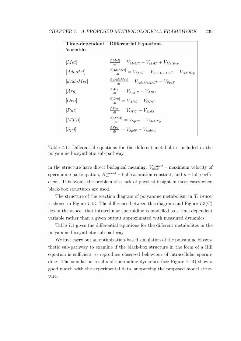
BIBLIOGRAPHY 293
Hu, X. and Eberhart, R. C.: 2002a, Adaptive particle swarm optimization: De-
tection and response to dynamic systems, Proceedings of the IEEE Congress
on Evolutionary Computation (CEC 2002), Hawaii, USA, pp. 1677–1681.
Hu, X. and Eberhart, R. C.: 2002b, Multiobjective optimization using dynamic
neighborhood particle swarm optimization, In Proceedings of the 2002 Con-
gess on Evolutionary Computation, part of the 2002 IEEE World Congress
on Computational Intelligence, IEEE Press, Hawaii, pp. 1–5.
Hua, S., Li, X., Coffino, P. and Wang, C. C.: 1995, Rat antizyme inhibits
the activity but does not promote the degradation of mouse ornithine de-
carboxylase in Trypanosoma brucei, The Journal of Biological Chemistry
270(17), 10264–10271.
Huang, C.-M., Huang, C.-J. and Wang, M.-L.: 2005, A particle swarm optimiza-
tion to identifying the armax model for short-term load forecasting, IEEE
transaction on power systems 20(2).
Huang, C.-Y. F. and Jr., J. E. F.: 1996, Ultrasensitivity in the mitogen-activated
protein kinase cascade, Proc. Natl. Acad. Sci. USA 93, 10078–10083.
Hunt, C. A., Ropella, G. E. P., Park, S. and Engelberg, J.: 2008, Dichotomies
between computational and mathematical models, Nature Biotechnology
26(7), 737–738.
Huynh, T. T., Huynh, V. T., Harmon, M. A. and Phillips, M. A.: 2003, Gene
knockdown of γ-glutamylcysteine synthetase by RNAi in the parasitic pro-
tozoa Trypanosoma brucei demonstrates that it is an essential enzyme, The
Journal of Biological Chemistry 278(41), 39794–39800.
Igoillo-Esteve, M., Maugeri, D., Stern, A. L., Beluardi, P. and Cazzulo, J. J.:
2007, The pentose phosphate in Trypanosoma cruzi: a potential target for
the chemotherapy of Chagas disease, Annals of the Brazilian Academy of
Sciences 79(4), 649–663.
Iniesta, V., Gomez-Nieto, L. C. and Corraliza, I.: 2001, The inhibition of
arginase by N-Hydroxy-L-Arginine controls the growth of leishmaina in-
side macrophages, The Journal of Experimental Medicine 193(6), 777–783.

BIBLIOGRAPHY 294
Jacquez, J. A. and Greif, P.: 1985, Numerical parameter identifiability and
estimability: integrating identifiability, estimability, and optimal sampling
design, Mathematical BioSciences 77, 201–227.
Jiang, Y., Roberts, S. C., Jardim, A., Carter, N. S., Shih, S., Ariyanayagam, M.,
Fairlamb, A. H. and Ullman, B.: 1999, Ornithine decarboxylase gene dele-
tion mutants of leishmania donovani, The Journal of Biological Chemistry
274(6), 3781–3788.
Jourdan, F., Breitling, R., Barrett, M. P. and Gilbert, D.: 2008, Metanetter:
inference and visualization of high-resolution metabolomic networks, Bioin-
formatics 24(1), 143–145.
Kaiser, A. E., Gottwald, A. M., Wiersch, C. S., Maier, W. A. and Seitz, H. M.:
2003, Spermidine metabolism in parasitic protozoa - a comparison to the sit-
uation in prokaryotes, viruses, plants and fungi, Folia parasitologica 50, 3–
18.
Kandpal, M., Fouce, R. B., Pal, A., Guru, P. Y. and Tekwani, B. L.: 1995,
Kinetics and molecular characteristics of arginine transport by Leishmania
donovani promastigotes, Molecular and Biochemical Parasitology 71, 193–
201.
Karp, P. D. and Mavrovouniotis, M. L.: 1994, Representing, analyzing, and
synthesizing biochemical pathways, IEEE Expert: Intelligent Systems and
Their Applications 09(2), 11–21.
Karp, P. D., Paley, S. and Romero, P.: 2002, The pathway tools software,
Bioinformatics 18, 225–232.
Kauffman, K. J., Prakash, P. and Edwards, J. S.: 2003, Advances in flux balance
analysis, Current Opinion in Biotechnology 14, 491–496.
Kaur, K., Emmett, K., McCann, P. P., Sjoerdsma, A. and Ullman, B.: 1986,
Effects of DL-alpha-difluoromethylornithine on leishmania donovani pro-
mastigotes, J. Protozool 33, 518–521.
Keiser, J., Stich, A. and Burri, C.: 2001, New drugs for the treatment of hu-
man African trypanosomiasis: research and development, Trends Parasitol
17(1), 42–49.

BIBLIOGRAPHY 295
Kelly, J. M., Taylor, M. C., Smith, K., Hunter, K. J. and Fairlamb, A. H.: 1993,
Phenotype of recombinant Leishmania donovani and Trypanosoma cruzi
which over-express trypanothione reductase, European Journal of Biochem-
istry 218, 29–37.
Kemna, A. H. and Mellichamp, D. A.: 1995, Identification of combined physical
and empirical models using nonlinear A Prior knowledge, Control Eng.
Practice 3(3), 375–382.
Kennedy, J. and Eberhart, R. C.: 1995, Particle swarm optimization, IEEE
International Conference on Neural Networks 4, 1942–1948.
Khan, M. O. F.: 2007, Trypanothione reductase: a viable chemotherapeutic
target for antitrypanosomal and antileishmanial drug desing, Drug Target
Insights 1, 129–146.
Kholodenko, B. N., Kiyatkin, A., Bruggeman, F. J., Sontag, E. and Westerhoff,
H. V.: 2002, Untangling the wires: A strategy to trace functional inter-
actions in signaling and gene networks, Proc. Natl. Acad. Sci. 99, 12841–
12846.
Kitano, H.: 2002a, Computational systems biology, Nature 420, 206–210.
Kitano, H.: 2002b, Systems biology: a brief overview, Science 295(5560), 1662–
1664.
Klamt, S. and Stelling, J.: 2003, Two approaches for metabolic pathway analy-
sis?, Trends in Biotechnology 21(2), 64–69.
Kocijan, J., Murray-Smith, R., Rasmussen, C. E. and Likar, B.: 2003, Predic-
tive control with gaussian process models, in B. Zajc and M. Tkal (eds),
Proceedings of IEEE Region 8 Eurocon 2003: Computer as a Tool, pp. 352–
356.
Koh, G., Teong, H. F. C., Clement, M.-V., Hsu, D. and Thiagarajan, P. S.: 2006,
A decompositional approach to parameter estimation in pathway modeling:
a case study of the Akt and MAPK pathways, Bioinformatics 22(14), e271–
e280.
Krauth-Siegel, R. L., Bauer, H. and Schirmer, R. H.: 2005, Dithiol proteins
as guardians of the intracellular redox milieu in parasites: old and new
BIBLIOGRAPHY 296
drug targets in trypanosomes and malaria-causing plasmodia, Angewandte
Chemie (International ed. in English) 44(5), 690–715.
Krauth-Siegel, R. L. and Comini, M. A.: 2008, Redox control in trypanoso-
matids, parasitic protozoa with trypanothione-based thiol metabolism,
Biochimica et biophysica acta 1780(11), 1236–1248.
Krauth-Siegel, R. L., Enders, B., Henderson, G. B., Fairlamb, A. H. and
Schirmer, R. H.: 1987, Trypanothione reductase from trypanosoma
cruzi purification and characterization of the crystalline enzyme, Eur. J.
Biochem. 164, 123–128.
Krauth-Siegel, R. L. and Inhoff, O.: 2003, Parasite-specific trypanothione re-
ductase as a drug target molecule, Parasitol Res 90, S77–S85.
Krieger, S., Schwarz, W., Ariyanayagam, M. R., Fairlamb, A. H., Krauth-Siegel,
R. L. and Clayton, C.: 2000, Trypanosomes lacking trypanothione reductase
are avirulent and show increased sensitivity to oxidative stress, Molecular
Microbiology 35(3), 542–552.
Krohling, R. A., Hoffmann, F. and dos Santos Coelho, L.: 2004, Co-evolutionary
particle swarm optimization for min-max problems using gaussian distribu-
tions, IEEE Transactions on Systems, Man and Cybernetics pp. 1407–1416.
Kropf, P., Fuentes, J. M., Fahnrich, E., Arpa, L., Herath, S., Weber, V., Soler,
G., Celada, A., Modolell, M. and Muller, I.: 2005, Arginase and polyamine
synthesis are key factors in the regulation of experimental leishmaniasis in
vivo, The FASEB Journal 19(8), 1–25.
Kumar, V. S., Dasika, M. S. and Maranas, C. D.: 2007, Optimization based auto-
mated curation of metabolic reconstructions, BMC Bioinformatics 8(1), 1–
16.
Kwon, D. S., Lin, C.-H., Chen, S., Coward, J. K., Walsh, C. T. and
J. Martin Bollinger, J.: 1997, Dissection of gluathionylspermidine syn-
thetase/amidase from escherichia coli into autonomously folding and func-
tional synthetase and amidase domains, The Journal of Biological Chem-
istry 272(4), 2429–2436.
Lauffenburger, D. A.: 2000, Cell signaling pathways as control modules: Com-
plexity for simplicity, PNAS 97(10), 5031–5033.

BIBLIOGRAPHY 297
Lauwers, L., Schoukens, J., Pintelon, R., Moer, W. V. and Gomme, L.: 2007,
Some practical applications of a nonlinear block structure identification pro-
cedure, Instrumentation and Measurement, Technology Conference, IMTC,
Warsaw, Poland, pp. 1–6.
Lee, K., Berthiaume, F., Stephanopoulos, G. N. and Yarmush, M. L.: 1999,
Metabolic flux analysis: a powerful tool for monitoring tissue function,
Tissue Engineering 5(4), 347–368.
Lewis, R. M. and Torczon, V.: 1996, Rank ordering and positive basis in pattern
search algorithms, Technical Report 71, ICASE NASA Langley Research
Center.
Li, H., Meininger, C. J., James R. Hawker, J., Haynes, T. E., Kepka-Lenhart, D.,
Mistry, S. K. and Sidney M. Morris, J.: 2001, Regulatory role of arginase i
and ii in nitric oxide, polyamine, and proline syntheses in endothelial cells,
Am J Physiol Endocrinol Metab 280, 75–82.
Liu, P. K. and Wang, F. S.: 2008, Inference of biochemical network models
in s-system using multi-objective optimization approach, Bioinformatics
pp. 1–7.
Liu, X., Jiang, J., Ajayi, O., Gu, X., Gilbert, D. and Sinnott, R.: 2008, Bionessie
– a grid enabled biochemical networks simulation environment, in S. et al.
(ed.), Global Healthgrid: e-Science Meets Biomedical Informatics – Pro-
ceedings of HealthGrid 2008, Vol. 138, pp. 147–157.
Liu, Y. and Yokota, H.: 2005, Modeling transcriptional regulation in chondro-
genesis using particle swarm optimization, CIBCB, pp. 311–317.
Ljung, L.: 2007, Some aspects on nonlinear black-box modeling in system iden-
tification, Technical report, Linkopings Universitet.
Ljung, L.: 2008, Perspective on system identification, Plenary Session, 17th
IFAC World Congress, Seoul, Korea.
Lueder, D. V. and Phillips, M. A.: 1996, Characterization of trypanosoma brucei
γ-glutamylcysteine synthetase, an essential enzyme in the biosynthesis of
trypanothione Diglutathionylspermidine, The Journal of Biological Chem-
istry 271(29), 17485–17490.

BIBLIOGRAPHY 298
Mamont, P. S., Danzin, C., Wagner, J., Siat, M., Joder-ohlenbusch, A.-M.
and Claverie, N.: 1982, Accumulation of decarboxylated S-Adenosyl-L-
Methionine in mammalian cells as a consequence of the inhibition of pu-
trescine biosynthesis, Eur. J. Biochem 123, 499–504.
Marton, L. J. and Pegg, A. E.: 1995, Polyamines as targets for therapeutic
intervention, Annual Reviews 35, 55–91.
Meierjohann, S., Walter, R. D. and Muller, S.: 2002, Glutathione synthetase
from plasmodium falciparum, Journal of Biochemistry 363, 833–838.
Mendes, P.: 1993, GEPASI: a software package for modelling the dynamics,
steady states and control of biochemical and other systems, Bioinformatics
9(5), 563–571.
Moles, C. G., Mendes, P. and Banga, J. R.: 2003, Parameter estimation in bio-
chemical pathways: A comparison of global optimization methods, Genome
Research 13, 2467–2474.
Morohashi, H., Winn, A. E., Borisuk, M. T., Bolouri, H., Doyle, J. and Kitano,
H.: 2002, Robustness as a measure of plausibility in models of biochemical
networks, Journal of Theoretical Biology 216, 19–30.
Mostaghim, S. and Teich, J.: 2003, Strategies for finding good local guides in
multi-objective particle swarm optimizers (mopso), In IEEE Swarm Intel-
ligence Symposium.
Muller, S., Liebau, E., Walter, R. D. and Krauth-Siegel, R. L.: 2003, Thiol-
based redox metabolism of protozoan parasites, Trends in Parasitology
19(7), 320–327.
Muller, T. G.: 2002, Modeling complex systems with differential equations, PhD
thesis, Albert-Ludwigs University.
Muller, T. G., Noykova, N., Gyllenberg, M. and Timmer, J.: 2002, Parame-
ter identifiability in dynamical models of anaerobic waste water treatment,
Mathematical Biosciences 177, 147–160.
Naka, S. and Fukuyama, Y.: 2001, Practical distribution state estimation using
hybrid particle swarm optimization, Proceeding of IEEE Power Engineer-
ing, Columbus, Ohio, USA.
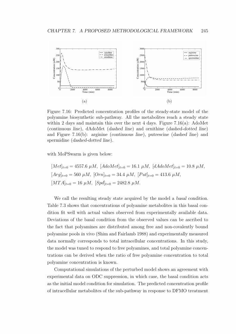
BIBLIOGRAPHY 299
Neelamkavil, F.: 1987, Computer Simulation and Modelling, John Wiley and
Sons.
Neves, S. R. and Iyengar, R.: 2002, Modeling of signaling networks, BioEssays
24, 1110–1117.
Newman, M. E. J.: 2001, Scientific collaboration networks. ii. shortest paths,
weighted networks, and centrality, Physical Review 64, 1–7.
Nogales, J., ∅ Palsson, B. and Thiele, I.: 2008, A genome-scale metabolic re-
construction of Pseudomonas putida kt2440: ijn746 as a cell factory, BMC
Systems Biology 2(1), 1–20.
Oancea, I.: 2003, Topological analysis of metabolic and regulatory networks by
decomposition methods, PhD thesis, Humboldt University, Berlin, Germany.
Opperdoes, F. R., Baudhuin, P., Coppens, I., Roe, C. D., Edwards, S. W., Wei-
jers, P. J. and Misset, O.: 1984, Purification, morphometric analysis, and
characterization of th glycosomes (microbodies) of the protozoan hemoflag-
ellate trypanosoma brucei, The Journal of Cell Biology 98, 1178–1184.
Orton, R. J., Sturm, O. E., Vyshemirsky, V., Calder, M., Gilbert, D. and Kolch,
W.: 2005, Computational modelling of the receptor-tyrosine-inase-activated
mark pathway, Biochemical Society 392, 249–261.
Osterman, A., Grishin, N. V., Kinch, L. N. and Phillips, M. A.: 1994, For-
mation of functional cross-species heterodimers of ornithine decarboxylase,
Biochemistry 33, 13662–13667.
Osyczka, A.: 1985, Multicriteria optimization for engineering design, In Design
Optimization, Springer.
Othmer, H. G.: 1980, The interaction of structure and dynamics in chemical
reaction networks, Proceedings of an international workshop, Heidelberg,
Germany.
Oussar, Y. and Dreyfus, G.: 2001, How to be a gray box: dynamics semi-physical
modeling, Neural Networks 14, 1161–1172.
Oza, S. L., Ariyanayagam, M. R., Aitcheson, N. and Fairlamb, A. H.: 2003,
Properties of trypanothione synthetase from trypanosoma brucei, Molecular
& Biochemical Parasitology 131, 25–33.

BIBLIOGRAPHY 300
Oza, S. L., Ariyanayagam, M. R. and Fairlamb, A. H.: 2002, Characterization
of recombinant glutathionylspermidine synthetase/amidase from crithidia
fasciculata, Journal of Biochemistry 364, 679–686.
Pant, M., Thangaraj, R. and Abraham, A.: 2008, Particle swarm optimization
using adaptive mutation, DEXA ’08: Proceedings of the 2008 19th Inter-
national Conference on Database and Expert Systems Application, IEEE
Computer Society, Washington, DC, USA, pp. 519–523.
Papin, J. A., Price, N. D., Wiback, S. J., Fell, D. A. and Palsson, B. O.: 2003,
Metabolic pathways in the post-genome era, Trends in Biochemical Science
28(5), 250–258.
Parsopoulos, K. E. and Vrahatis, M. N.: 2002a, Particle swarm optimization
method in multiobjective problems, In Proceedings of the 2002 ACM Sym-
posium on Applied Computing (SAC 2002), pp. 603–607.
Parsopoulos, K. E. and Vrahatis, M. N.: 2002b, Recent approaches to global
optimization problems through particle swarm optimizaiton, Natural Com-
puting 1, 225–230.
Pegg, A. E. and Jacobs, G.: 1983, Comparison of inhibitors of S-
adenosylmethionine decarboxylase from different species, Biochemistry
213, 495–502.
Peluffo, G., Piacenza, L., Irigoin, F., Alvarez, M. N. and Radi, R.: 2004, L-
arginine metabolism during interaction of trypanosoma cruzi with host cells,
Trends in Parasitology 20(8), 363–369.
Penketh, P. G. and Klein, R. A.: 1986, Hydrogen peroxide metabolism in try-
panosoma brucei, Molecular and Biochemical Parasitology 20, 111–121.
Pereira, C. A., Alonso, G. D., Ivaldi, S., Alves, A. S. M. J. M., Bouvier,
L. A., Flawia, M. M. and Torres, H. N.: 2002, Arginine metabolism in
trypanosoma cruzi is coupled to parasite stage and replication, FEBS Let-
ters 526, 111–114.
Persson, L.: 2007, Ornithine decarboxylase and S-adenosylmethionine decar-
boxylase in trypanosomatids, Biochemical Society Transactions 35, 314–
317.

BIBLIOGRAPHY 301
Persson, L., Jeppsson, A. and Nasizadeh, S.: 2003, Turnover of trypanosomal
ornithine decarboxylases, Biochemical Society Transactions 31, 411–414.
Peter S. Backlund, J., Chang, C. P. and Smith, R. A.: 1982, Identification of
2-Keto-4-methylthiobutyrate as an intermediate compound in methionine
synthesis from 5’-Methylthioadenosine, The Journal of Biological Chemistry
257(8), 4196–4202.
Peter S. Backlund, J. and Smith, R. A.: 1981, Methionine synthesis from
5’-methylthioadenosine in rat liver, The Journal of Biological Chemistry
256(4), 1533–1535.
Pfeiffer, T., Sanchez-Valdenebro, I., Nuno, J. C., Montero, F. and Schuster, S.:
1999, Metatool: for studying metabolic networks, Bioinformatics 15(3).
Phillips, M. A., Coffino, P. and Wang, C. C.: 1987, Cloning and sequencing of
the ornithine decarboxylase gene from trypanosoma brucei, The Journal of
Biological Chemistry 262(18), 8721–8727.
Phillips, M. A., Coffino, P. and Wang, C. C.: 1988, Trypanosoma brucei ornithine
decarboxylase: enzyme purification, characterization, and expression in es-
cherichia coli, The Journal of Biological Chemistry 263(34), 17933–17941.
Phillips, M. A. and Wang, C. C.: 1987, A Trypanosoma brucei mutant resis-
tant to α-difluoromethylornithine, Molecular and Biochemical Parasitology
22, 9–17.
Porter, C. W. and Sufrin, J. R.: 1986, Interference with polyamine biosynthe-
sis and/or function by analogs of polyamines or methionine as a potential
anticancer chemotherapeutic strategy, Anticancer Res. 6(4), 525–542.
Press, W. H., Teukolsky, S. A., Vetterling, W. T. and Flannery, B. P.: 2002,
Numerical Recipes in C: The Art of Scientific Computing, Cambridge Uni-
versity Press, Cambridge, UK.
Quesne, S. A. L. and Fairlamb, A. H.: 1996, Regulation of a high-affinity di-
amine transport system in Trypanosoma cruzi epimastigotes, Journal of
Biochemistry 316, 481–486.

BIBLIOGRAPHY 302
Rabbani, M., Bajestani, M. A. and Khoshkhou, G. B.: 2009, A multi-objective
particle swarm optimization for project selection problem, Expert Systems
with Applications .
Raman, K., Rajagopalan, P. and Chandra, N.: 2005, Flux balance analysis of
mycolic acid pathway: targets for anti-tubercular drugs, PLOS Computa-
tional Biology 1, 349–358.
Raquel, C. R. and Naval, P. C.: 2005, An effective use of crowding distance
in multiobjective particle swarm optimization, GECCO ’05: Proceedings of
the 2005 conference on Genetic and evolutionary computation, ACM, New
York, NY, USA, pp. 257–264.
Ravasz, E., Somera, A. L., Mongru, D. A., Oltvai, Z. N. and Barabasi, A. L.:
2002, Hierarchical organization of modularity in metabolic networks, Sci-
ence 297, 1551–1555.
Reed, J. L., Patel, T. R., Chen, K. H., Joyce, A. R., Applebee, M. K., Herring,
C. D., Bui, O. T., Knight, E. M., Fong, S. S. and ∅ Palsson, B.: 2006,
Systems approach to refining genome annotation, PNAS 103(46), 17480–
17484.
Reed, M. C., Thomas, R. L., Pavisic, J., James, S. J., Ulrich, C. M. and Nijhout,
H. F.: 2008, A mathematical model of glutathione metabolism, Theoretical
Biology and Medical Modelling 5(8), 1–16.
Reguera, R. M., Balana-Fouce, R., Perez-Pertejo, Y., Fernandez, F. J., Garcia-
Estrada, C., Cubria, J. C. and an David Ordonez, C. O.: 2001, Cloning
expression and characterization of methionine adenosyltransferase in Leish-
mania infantum promastigotes, The Journal of Biological Chemistry pp. 1–
40.
Reguera, R. M., Redondo, C. M., Perez-Pertejo, Y. and Balana-Fouce, R.: 2007,
S-adenosymethionine in protozoan parasites: Functions, synthesis and reg-
ulation, Molecular & Biochemical Parasitology 152, 1–10.
Reyes-Sierra, M. and Coello, C. A. C.: 2006, Multi-objective particle swarm
optimizers: A survey of the state-of-the-art, International Journal of Com-
putational Intelligence Research 2(3), 287–308.

BIBLIOGRAPHY 303
Riscoe, M. K., Ferro, A. J. and Fitchen, H.: 1989, Methionine recycling as a
target for antiprotozoal drug development, Parasitology Today 5(10), 330–
333.
Roberts, S. C., Jiang, Y., Gasteier, J., Frydman, B., Marton, L. J., Heby, O.
and Ullman, B.: 2007, Leishmania donovani polyamine biosynthetic en-
zyme overproducers as tools to investigate the mode of action of cytotoxic
polyamine analogs, Antimicrobial Agents and Chemotherapy 51(2), 438–
445.
Roberts, S. C., Jiang, Y., Jardim, A., Carter, N. S., Heby, O. and Ullman, B.:
2001, Genetic analysis of spermidine synthase from leishmania donovani,
Molecular and Biochemical Parasitology 115(2), 217–226.
Roberts, S. C., Scott, J., Gasteier, J. E., Jiang, Y., Brooks, B., Jardim, A.,
Carter, N. S., Heby, O. and Ullman, B.: 2002, S-Adenosylmethionine de-
carboxylase from leishmania donovani, The Journal of Biological Chemistry
277(8), 5902–5909.
Roberts, S. C., Tancer, M. J., Polinsky, M. R., Gibson, K. M., Heby, O.
and Ullman, B.: 2004, Arginase plays a pivotal role in polyamine pre-
cursor metabolism in leishmaina, The Journal of Biological Chemistry
279(22), 23668–23678.
Rodriguez-Caso, C., Montanez, R., Cascante, M., Sanchez-Jimenez, F. and Med-
ina, M. A.: 2006, Mathematical modelling of polyamine metabolism in
mammals, The Journal of Biological Chemistry 281(31), 21799–21812.
Rodriguze-Fernandez, M., Egea, J. A. and Banga, J. R.: 2006, Novel meta-
heuristic for parameter estimation in nonlinear dynamic biological systems,
BMC Bioinformatics 7.
Sauro, H. M., Uhrmacher, A. M., Harel, D., Hucka, M., Kwiatkowska, M.,
Mendes, P., Shaffer, C. A., Stromback, L. and Tyson, J. J.: 2006, Challenges
for modeling and simulation methods in systems biology, in L. F. Perrone,
F. P. Wieland, J. Liu, B. G. Lawson, D. M. Nicol and R. M. Fujimoto (eds),
Proceedings of the 2006 Winter Simulation Conference, pp. 1720–1730.

BIBLIOGRAPHY 304
Schilling, C. H., Edwards, J. S., Letscher, D. and Palsson, B.: 2000, Combining
pathway analysis with flux balance analysis for the comprehensive study of
metabolic systems, Biotechnology and Bioengineering 71(4), 286–306.
Schirmer, R. H., Schollhammer, T., Eisenbrand, G. and Krauth-Siegel, R. L.:
1987, Oxidative stress as a defense mechanism against parasitic infections,
Free Rad. Res. Comms. 3(1-5), 3–12.
Schmidt, H. and Krauth-Siegel, R. L.: 2003, Functional and physicochemical
characterization of the thioredoxin systems in Trypanosoma brucei, The
Journal of Biological Chemistry 278(47), 46329–46336.
Schness, S. and Mendoze, C.: 1997, Closed form solution for time-dependent
enzyme kinetics, Journal of Theoretical Biology 187, 207–212.
Schoeberl, B., Eichler-Jonsson, C., Gilles, E. D. and Muller, G.: 2002, Compu-
tational modeling of the dynamics of the MAP kinase cascade activated by
surface and internalized EGF receptors, Nature Biotechnology 20, 370–375.
Schuster, S., Dandekar, T. and Fell, D. A.: 1999, Detection of elementary flux
modes in biochemical networks: a promising tool for pathway analysis and
metabolic engineering, Trends in Biotechnology 17, 53–60.
Schuster, S., Fell, D. A. and Dandekar, T.: 2000, A general definition of
metabolic pathways useful for systematic organization and analysis of com-
plex metabolic networks, Nature Biotechnology 18, 326–332.
Schuster, S., Hilgetag, C., Woods, J. H. and Fell, D. A.: 2002, Reaction routes
in biochemical reaction systems: Algebraic properties, validated calculation
procedure and example from nucleotide metabolism, Journal of Mathemat-
ical Biology 45, 153–181.
Schuster, S., Klamt, S., Weckwerth, W., Moldenhauer, F. and Pfeiffer, T.: 2002,
Use of network analysis of metaboli systems in bioengineering, Bioprocess
biosyst Eng 22, 363–372.
Schuster, S. and Schusters, R.: 1990, Detecting strictly detailed balanced subnet-
works in open chemical reaction networks, Journal of Mathematical Chem-
istry 6, 17–40.

BIBLIOGRAPHY 305
Schutte, J. F., Reinbolt, J. A., Fregly, B. J., Haftka, R. T. and George, A. D.:
2003, Parallel global optimization with the particle swarm algorithm, Jour-
nal of Numerical Methods in Engineering 61, 2296–2315.
Schwartz, J.-M. and Kanehisa, M.: 2005, A quadratic programming approach
for decomposing steady-state metabolic flux distributions onto elementary
modes, Bioinformatics 21(Suppl. 2), ii204–ii205.
Schwartz, J.-M. and Kanehisa, M.: 2006, Quantitative elementary mode analysis
of metabolic pathways: the example of yeast glycolysis, BMC Bioinformat-
ics 7(186), 1–20.
Soderstrom, T. and Stoica, P.: 1989, System Identification, Prentice Hall.
Sjoberg, J., Zhang, Q., Ljung, L., Benveniste, A., Delyon, B., Glorennec, P.,
Hjalmarsson, H. and Juditsky, A.: 1995, Nonlinear black-box modeling in
system identification: a unified overview, Automatica 31, 1691–1724.
Selamnia, M., Mayeur, C., Robert, V. and Blachier, F.: 1998, α-
difluoromethylornithine (DFMO) as a potent arginase activity inhibitor in
human colon carcinoma cells, Biochemical Pharmacology 55, 1241–1245.
Selzer, P. M., Hesse, F., Hamm-Kunzelmann, B., Muhlstadt, K., Echner, H.
and Duszenko, M.: 1996, Down regulation of S-adenosylmethionine decar-
boxylase activity of trypanosoma brucei brucei during transition from long
slender to short stumpy-like forms in axenic culture, Eur. J. Cell Biol.
99, 173–179.
Shampine, L. F., Kierzenka, J. A. and Reichelt, M. W.: 2000,
Solving boundary value problems for ordinary differential equa-
tions in matlab with bvp4c, p. 27pp. Manuscript, available at
http://www.mathworks.com/bvp tutorial.
Shankland, C., Tran, N., Baral, C. and Kolch, W.: 2005, Reasoning about
the erk signal transduction pathway using BioSigNet-RR, In proceedings of
Computational Methods in Systems Biology, CMSB, Informal publication,
pp. 79–90.
Shi, Y. and Eberhart, R. C.: 1998, Parameter selection in particle swarm opti-
mization, Lecture Notes in Computer Science 1447, 591–600.

BIBLIOGRAPHY 306
Shim, H. and Fairlamb, A. H.: 1988, Levels of polyamines, glutathione and
glutathione-spermidine conjugates during growth of the insect Trypanoso-
matid Crithidia fasciculata, Journal of General Microbiology 134, 807–817.
Sidney M. Morris, J.: 2002, Regulation of enzymes of the urea cycle and arginine
metabolism, Annu. Rev. Nutr. 22, 87–105.
Silva, E. R., Silva, M. F. L., Fischer, H., Mortara, R. A., Mayer, M. D.,
Framesqui, K., Silber, A. M. and Floeter-Winter, L. M.: 2007, Biochemi-
cal and biophysical properties of a highly active recombinant arginase from
leishmania (leishmania) amazonensis and subcellular localization of native
enzyme, Molecular & Biochemical Parasitology 159(2), 104–111.
Smith, A. E. and Coit, D. W.: 1997, Handbook of Evolutionary Computation,
Joint Publication of Oxford University Press and Institute of Physics Pub-
lishing, chapter Section C5.2, Penalty Functions.
Sontag, E. D.: 2005, Molecular systems biology and control: A qualitative-
quantitative approach, In Decision and Control, European Control Confer-
ence CDC-ECC’05, pp. 2314–2319.
Sontag, E. D.: 2006, Some remarks on input choices for biochemi-
cal systems, Optimization and Control (math.OC) . Available at
http://arxiv.org/abs/math/0606261v1.
Sontag, E., Kiyatkin, A. and Kholodenko, B. N.: 2004, Inferring dynamic ar-
chitecture of cellular networks using time series of gene expression, protein
and metabolite data, Bioinformatics 20(12), 1877–1886.
Srividhya, J., Schnell, S., Crampin, E. J. and E., P.: 2007, Reconstructing
biochemical pathways from time course data, Proteomics 7, 828–838.
Stelling, J., Klamt, S., Bettenbrock, K., Schuster, S. and Gilles, E. D.: 2002,
Metabolic network structure determines key aspects of functionality and
regulation, Nature 420, 190–193.
Stephanopoulos, G.: 1999, Metabolic fluxes and metabolic engineering,
Metabolic Engineering 1, 1–11.

BIBLIOGRAPHY 307
Stephanopoulos, G. N., Aristidou, A. A. and Nielsen, J.: 1998, Metabolic Engi-
neering: Principles and Methodologies, Academic Press, California, USA,
chapter 8: Metabolic Flux Analysis, pp. 309–351.
Sufrin, J. R., Meshnick, S. R., Spiess, A. J., Garofalo-Hannan, J., Pan, X.-Q.
and Bacchi, C. J.: 1995, Methionine recycling pathways and antimalarial
drug design, Antimicrobial Agents and Chemotherapy 39(11), 2511–1515.
Sufrin, J. R., Spiess, A. J., Canio J. Marasco, J., Rattendi, D. and Bacchi, C. J.:
2008, Novel trypanocidal analogs of 5’-(methylthio)-adenosine, Antimicro-
bial Agents and Chemotherapy 52(1), 211–219.
Swameye, I., Muller, T. G., Timmer, J., Sandra, O. and Klingmuller, U.: 2003,
Identification of nucleocytoplasmic cycling as a remote sensor in cellular
signaling by databased modeling, Proc. Natl. Acad. Sci. 100(3), 1028–1033.
Takors, R., Wiechert, W. and Weuster-Botz, D.: 1997, Experimental design
for the identification of macrokinetic models and model discrimination,
Biotechnology and Bioengineering 56(5), 565–576.
Tan, K. C. and Li, Y.: 2002, Grey-box model identification via evolutionary
computing, Control Engineering Practice 10(7), 673–684.
Taylor, M. C., Kaur, H., Blessington, B., Kelly, J. M. and Wilkinson, S. R.: 2008,
Validation of spermdine synthase as a drug target in african trypanosomes,
Biochem. J 409, 563–569.
Tekwani, B. L., Bacchi, C. J. and Pegg, A. E.: 1992, Putrescine activated S-
adenosylmethionine decarboxylase from trypanosoma brucei brucei, Molec-
ular and Cellular Biochemistry 117, 53–61.
Thacker, W. C.: 1989, The role of the Hessian matrix in fitting models to
measurements, Journal of Geophysical Research 94(C5), 6177–6196.
Thieffry, D. and Thomas, R.: 1998, Qualitative analysis of gene networks, in
R. B. Altman, A. K. Dunker, L. Hunter and T. E. Klein (eds), Pacific
Symposium on Biocomputing, Vol. 3, Singapore, pp. 77–88.
Torczon, V.: 1997, On the convergence of pattern search algorithms, SIAM
Journal on Optimization 7(1), 1–25.
BIBLIOGRAPHY 308
Tulleken, H.: 1993, Grey-box modelling and identification using physical knowl-
edge and bayesian techniques, Automatica 29(2), 285–308.
Tulleken, H. J. A. F.: 1991, Application of the grey-box approach to parameter
estimation in physicochemical models, Proceedings of the 30th Conference
on Decision and Control, Brighton, England.
Turnock, D. C. and Ferguson, M. A. J.: 2007, Sugar nucleotide pools of Try-
panosoma brucei, Trypanosoma cruzei, and Leishmania major, Eukaryotic
Cell 6(8), 1450–1463.
Turrens, J. F.: 2004, Oxidative stress and antioxidant defense: a target for the
treatment of diseases caused by parasitic protozoa, Molecular Aspects of
Medicine 25, 211–220.
Tyson, J. J., Chen, K. C. and Novak, B.: 2003, Sniffers, buzzers, toggles and
blinkers: dynamics of regulatory and signalling pathways in the cell, Cur-
rent Opinion in Cell Biology 15, 221–231.
Ullah, M., Schmidt, H., Cho, K.-H. and Wolkenhauer, O.: 2006, Deterministic
modelling and stochastic simulation of biochemical pathways using matlab,
Systems Biology 153, 53–60.
van den Bergh, F.: 2001, An Analysis of Particle Swarm Optimizers, PhD thesis,
University of Pretoria.
van den Bergh, F. and Engelbrecht, A. P.: 2004, A cooperative approach to par-
ticle swarm optimization, IEEE transactions on evolutionary computation
8(3).
van Riel, N. A. W.: 2006, Dynamic modelling and analysis of biochemical net-
works: mechanism-based models and model-based experiments, Briefings
in Bioinformatics 7, 364–374.
van Riel, N. A. W. and Sontag, E. D.: 2006, Parameter estimation in mod-
els combining signal transduction and metabolic pathways: the dependent
input approach, IEE Proceeding Systems Biology 153(4), 263–274.
Varma, A. and Palsson, B. O.: 1993, Metabolic capabilities of Escherichia coli:
synthesis of biosynthetic precursors and cofactors, Journal of Theoretical
Biology 165(4), 477–502.

BIBLIOGRAPHY 309
Varma, A. and Palsson, B. O.: 1994, Metabolic flux balancing: Basic concepts,
scientific and practical use, Nature 12, 994–998.
Vaz, A. I. F. and Vicente, L. N.: 2007, A particle swarm pattern search method
for bound constrained global optimization, Journal of Global Optimization
39, 197–219.
Vina, J. R., Palacin, M. and Puertes, I. R.: 1989, Role of the γ-glutamyl cycle
in the regulation of amino acid translocation, The American Journal of
Physiology 257, E916–E922.
Vincendeau, P., Gobert, A. P., Daulouede, S., Moynet, D. and Mossalayi, M. D.:
2003, Arginases in parasitic diseases, Trends in Parasitology 19(1), 9–12.
Voit, E. O.: 2000, Computational Analysis of Biochemical Systems: A Practi-
cal Guide for Biochemists and Molecular Biologists, Cambridge University
Press.
von Dassow, G., Meir, E., Munro, E. M. and Odell, G. M.: 2000, The segment
polarity network is a robust developmental module, Nature 406, 188–192.
von Kamp, A. and Schuster, S.: 2006, Metatool 5.0: fast and flexible elementary
modes analysis, Bioinformatics 22(15).
Vyshemirsky, V.: 2007, Probabilistic Reasoning and Inference for Systems Biol-
ogy, PhD thesis, The University of Glasgow, Glasgow, UK.
Wallace, H. M.: 1996, Polyamines in human health, Proceedings of the Nutrition
Society, Vol. 55, pp. 419–431.
Wallace, H. M. and Fraser, A. V.: 2004, Inhibitors of polyamine metabolism:
review article, Amino Acids 26, 353–365.
Wessels, L. F. A., Someren, E. P. V. and Reinders, M. J. T.: 2001, A comparison
of genetic network models, Pacific Symposium on Biocomputing, pp. 508–
519.
Westerhoff, H. V., Kolodkin, A., Conradie, R., Wilkinson, S. J., Bruggeman,
F. J., Krab, K., van Schuppen, J. H., Hardin, H., Bakker, B. M., Mone,
M. J., Rybakova, K. N., Eijken, M., van Leeuwen, H. J. P. and Snoep, J. L.:
2009, Systems biology towards life in silico: mathematics of the control of
living cells, Journal of mathematical biology 58, 7–34.

BIBLIOGRAPHY 310
Wiechert, W.: 2001, 13c metabolic flux analysis, Metabolic Engineering 3, 195–
206.
Wiechert, W.: 2002, Modeling and simulation: tools for metabolic engineering,
Journal of Biotechnology 94, 37–63.
Wilhelm, T., Behre, J. and Schuster, S.: 2004, Analysis of structural robustness
of metabolic networks, IEE Proc. Syst. Biol. 1(1), 114–120.
Willert, E. K., Fitzpatrick, R. and Phillips, M. A.: 2007, Allosteric regulation of
an essential trypanosome polyamine biosynthetic enzyme by a catalytically
dead homolog, PNAS 104(20), 8275–8280.
Willert, E. K. and Phillips, M. A.: 2008, Regulated expression of an essential al-
losteric activator of polyamine biosynthesis in African Trypanosomes, PLoS
Pathogens 4, 1–12.
Wolkenhauer, O., Ullah, M., Wellstead, P. and Cho, K.: 2004, The dynamic
systems approach to control and regulation of intracellular networks, FEBS
Letters 579, 1846–1853.
Wu, G. and Sidney M. Morris, J.: 1998, Arginine metabolism: nitric oxide and
beyond, Biochemistry 336, 1–17.
Xiao, Y., McCloskey, D. E. and Phillips, M. A.: 2009, Rna inference-mediated
silencing of ornithine decarboxylase and spermidine synthase genes in Try-
panosoma brucei provides insight into regulation of polyamine biosynthesis,
Eukaryotic Cell 8(5), 747–755.
Yarlett, N. and Bacchi, C. J.: 1988, Effect of dl-α-difluoromethylorinthine on
methionine cycle intermediates in trypanosoma brucei brucei, Molecular and
Biochemical Parasitology 27, 1–10.
Yarlett, N., Garofalo, J., Goldberg, B., Ciminelli, M. A., Ruggiero, V., Sufrin,
J. R. and Bacchi, C. J.: 1993, S-adenosylmethionine synthetase in blood-
stream Trypanosoma brucei, Biochim Biophys Acta 24(1), 68–76.
Yarlett, N., Quamina, A. and Bacchi, C. J.: 1991, Protein methylase
in Trypanosoma brucei brucei: activities and response to DL-alpha-
difluoromethylornithine, Journal of General Microbiology 137(3), 717–724.

BIBLIOGRAPHY 311
Yoshida, H., Kawata, K., Fukuyama, Y. and Yoshida, H.: 1999, A particle swarm
optimization for reactive power and voltage control considering voltage sta-
bility, Proceedings of the International Conference on Intelligent System
Application to Power Systems (ISAP’99), Rio de Janeiro, Brazil, pp. 117–
121.
Zak, D. E., Gonye, G. E., Schwaber, J. S. and Doyle, F. J.: 2003, Importance of
input perturbations and stochastic gene expression in the reverse engineer-
ing of genetic regulatory networks: insights from an identifiability analysis
of an in silico network, Genome Research 13, 2396–2405.
Zhao, J., Ding, G.-H., Tao, L., Yu, H., Yu, Z.-H., Luo, J. H., Gao, Z.-W.
and Li, Y.-X.: 2007, Modular co-evolution of metabolic networks, BMC
Bioinformatics 8(311), 1–12.