ĠSTANBUL TECHNICAL UNIVERSITY INSTITUTE OF …polen.itu.edu.tr/bitstream/11527/4674/1/11629.pdf ·...
139
ĠSTANBUL TECHNICAL UNIVERSITY INSTITUTE OF SCIENCE AND TECHNOLOGY M.Sc. Thesis by Aykut CEYHAN Department : Aeronautical&Astronautical Engineering Programme : Interdisciplenary programme June 2011 UNMANNED HELICOPTER PRE-DESIGN AND ANALYSIS
Transcript of ĠSTANBUL TECHNICAL UNIVERSITY INSTITUTE OF …polen.itu.edu.tr/bitstream/11527/4674/1/11629.pdf ·...

ĠSTANBUL TECHNICAL UNIVERSITY INSTITUTE OF SCIENCE AND TECHNOLOGY
M.Sc. Thesis by
Aykut CEYHAN
Department : Aeronautical&Astronautical Engineering
Programme : Interdisciplenary programme
June 2011
UNMANNED HELICOPTER PRE-DESIGN AND ANALYSIS


ĠSTANBUL TECHNICAL UNIVERSITY INSTITUTE OF SCIENCE AND TECHNOLOGY
M.Sc. Thesis by
Aykut CEYHAN
(511091124)
Date of submission : 06 May 2011
Date of defence examination: 08 June 2011
Supervisor (Chairman) : Assoc. Prof. Dr. Vedat Z. DOĞAN (ITU)
Members of the Examining Committee : Prof. Dr. Zahit MECĠTOĞLU(ITU)
Prof. Dr. Tuncer TOPRAK(ITU)
June 2011
UNMANNED HELICOPTER PRE-DESIGN AND ANALYSIS


Haziran 2011
ĠSTANBUL TEKNĠK ÜNĠVERSĠTESĠ FEN BĠLĠMLERĠ ENSTĠTÜSÜ
YÜKSEK LĠSANS TEZĠ
Aykut CEYHAN
(511091124)
Tezin Enstitüye Verildiği Tarih : 06 Mayıs 2011
Tezin Savunulduğu Tarih : 08 Haziran 2011
Tez Danışmanı : Doç. Dr. Vedat Ziya DOĞAN (ĠTÜ)
Diğer Jüri Üyeleri : Prof. Dr. Zahit MECĠTOĞLU (ĠTÜ)
Prof. Dr. Tuncer TOPRAK (ĠTÜ)
ĠNSANSIZ HELĠKOPTER ÖN TASARIMI VE ANALĠZĠ


v
FOREWORD
I would like to express my deep appreciation and thanks for my supervisor Assoc.
Prof. Dr. Vedat Ziya Doğan and my family for their support.
June 2011
Aykut Ceyhan
Aeronatical&Astronautical Engineering

vi

vii
TABLE OF CONTENTS
Page
TABLE OF CONTENTS ......................................................................................... vii ABBREVIATIONS ................................................................................................... ix
LIST OF TABLES .................................................................................................... xi LIST OF FIGURES ................................................................................................ xiii SUMMARY .............................................................................................................. xv
ÖZET ....................................................................................................................... xvii 1. INTRODUCTION .............................................................................................. 1
1.1. Purpose ......................................................................................................... 1 1.2. Similar design .............................................................................................. 2
2. CONCEPTUAL DESIGN ................................................................................. 3 2.1. Introduction .................................................................................................. 3
2.2. Mission requirements ................................................................................... 3 2.3. Payload ......................................................................................................... 4 2.4. Main rotor configuration .............................................................................. 8
2.4.1. Single rotor ........................................................................................... 8 2.4.2. Coaxial rotor......................................................................................... 9
2.4.3. Tandem rotor ...................................................................................... 10 2.4.4. Selection of main rotor configuration ................................................ 10
2.5. Tail rotor configuration .............................................................................. 11
2.5.1. Conventional tail rotor ....................................................................... 11
2.5.2. Notar ................................................................................................... 12 2.5.3. Fan-in-fin ........................................................................................... 12
2.5.4. Selection of tail rotor configuration ................................................... 13 2.6. Hub configuration ...................................................................................... 14
2.6.1. Teetering rotor .................................................................................... 14
2.6.2. Fully-articulated rotor ........................................................................ 15 2.6.3. Hingeless rotor ................................................................................... 15
2.6.4. Bearingless rotor ................................................................................ 15 2.6.5. Selection of hub.................................................................................. 15
2.7. Landing gear configuration ........................................................................ 16 2.8. Empennage ................................................................................................. 16 2.9. Engine ........................................................................................................ 16
2.10. Mission overview and pre-work on design ................................................ 17
2.11. Mission requirements ................................................................................. 20
3. MAIN ROTOR DESIGN ................................................................................. 21 3.1. First estimation of gross weight ................................................................. 21 3.2. Gross weight iteration ................................................................................ 33 3.3. Power required to hover IGE ..................................................................... 37 3.4. Power calculations at forward flight .......................................................... 38 3.5. Twist rate calculation with BEMT ............................................................. 46

viii
4. TAIL ROTOR DESIGN .................................................................................. 53 4.1. Preliminary tail rotor geometry .................................................................. 53 4.2. Power required ........................................................................................... 54
4.2.1. Power required at hover ..................................................................... 54
4.2.2. Power required at forward flight ........................................................ 58
5. TOTAL POWER CALCULATIONS AND ENGINE SELECTION .......... 61 5.1. Total power calculations ............................................................................ 61
5.1.1. Total power required for hover and forward flight ............................ 61 5.1.2. Required shaft power ......................................................................... 63
5.1.3. Required total engine shaft power ...................................................... 63 5.2. Engine selection ......................................................................................... 63
6. DESIGN FOR SELECTED ENGINE ............................................................ 67 6.1. Main rotor design ....................................................................................... 67 6.2. Tail rotor design ......................................................................................... 85
6.3. Total power calculations ............................................................................ 90
7. PERFORMANCE ANALYSIS ....................................................................... 93 7.1. Effect of density altitude ............................................................................ 93 7.2. Lift-to-Drag Ratios ..................................................................................... 93 7.3. Climb performance ..................................................................................... 94 7.4. Fuel consumption of the engine ................................................................. 99
7.5. Speed for minimum power and best endurance ....................................... 100 7.6. Speed for maximum range ....................................................................... 101 7.7. Ceiling ...................................................................................................... 102
8. VISUAL DESIGN WITH CATIA ................................................................ 105 8.1. Main rotor ................................................................................................. 105
8.2. Tail rotor ................................................................................................... 107 8.3. Fuselage .................................................................................................... 108
9. CONCLUSION ............................................................................................... 115 REFERENCES ....................................................................................................... 117
CURRICULUM VITAE ........................................................................................ 119

ix
ABBREVIATIONS
BEMT : Blade element momentum theory
BET : Blade element theory
BL : Blade loading
DL : Disk loading
EO : Electro-optical
GW : Gross weight
IGE : In ground effect
IR : Infrared
NOTAR : No tail rotor
OGE : Out of ground effect
PL : Payload
RPM : Revolution per minute
UL : Useful load

x

xi
LIST OF TABLES
Page
Table 2.1 : Trade study for rotors ............................................................................. 11 Table 2.2 : Trade study for tail rotor ........................................................................ 14
Table 2.3 : Trade study for hub ................................................................................ 16 Table 2.4 : Specifications of first engine.................................................................. 17 Table 2.5 : First approach to geometric quantities ................................................... 18 Table 2.6 : Mission requirements ............................................................................. 20
Table 3.1 : Disk loading data for similar helicopters ............................................... 22 Table 3.2 : Advance ratio blade loading coefficient variation ................................. 24 Table 3.3 : Inputs for Reynolds calculator ............................................................... 29
Table 3.4 : Profile drag coefficients with respect to Reynolds numbers for VR7 ... 30 Table 3.5 : Determination of Reynolds number at r=0.2 ......................................... 30
Table 3.6 : First gross weight iteration ..................................................................... 34 Table 3.7 : Determination of drag coefficient at blade stations at sea level ............ 36 Table 3.8 : Determination of drag coefficient at blade stations at 2000 meters ....... 36
Table 3.9 : Average profile drag coefficients ........................................................... 36 Table 3.10: Forward flight power calculator ............................................................. 40
Table 3.11: Induced velocity iteration....................................................................... 42 Table 3.12: Revised induced power values at sea level ............................................ 43 Table 3.13: Revised induced power values at 2000 meters ...................................... 43
Table 3.14: Power values at forward flight at sea level ............................................ 44
Table 3.15: Power values at forward flight at 2000 meters ...................................... 44 Table 3.16: Tip mach number at sea level ................................................................ 45
Table 3.17: Tip mach number at 2000 meters ........................................................... 46 Table 3.18: Modified momentum theory output of BEMT calculator ...................... 47 Table 3.19: BET output of BEMT calculator up to seven degrees ........................... 47
Table 3.20: BET output of BEMT calculator between 7 and 15 degrees twist angle48 Table 3.21: Input of BEMT ....................................................................................... 50
Table 3.22: Output of BEMT .................................................................................... 50 Table 3.23: Total power with BEMT ........................................................................ 51 Table 3.24: Helicopter's specifications ..................................................................... 52 Table 4.1 : Tail rotor power for untwisted main rotor blades at sea level ............... 55 Table 4.2 : Tail rotor power for untwisted main rotor blades at 2000 meters .......... 56
Table 4.3 : Tail rotor power for twisted main rotor blades at sea level ................... 57
Table 4.4 : Tail rotor power for twisted main rotor blades at 2000 meters .............. 57
Table 4.5 : Tail rotor power at forward flight at sea level ....................................... 58 Table 4.6 : Tail rotor power at forward flight at 2000 meters .................................. 59 Table 5.1 : Total power at hover .............................................................................. 61 Table 5.2 : Total power at forward flight at sea level .............................................. 62 Table 5.3 : Total power at forward flight at 2000 meters ........................................ 62 Table 5.4 : Comparison of power values ................................................................. 63 Table 5.5 : Engine database ..................................................................................... 65

xii
Table 5.6 : Specifications of selected engine ........................................................... 66
Table 6.1 : Geometric specifications of design before last iteration ........................ 69 Table 6.2 : Weight of design .................................................................................... 69 Table 6.3 : New gross weight iteration ..................................................................... 70
Table 6.4 : Last geometric specifications of design ................................................. 70 Table 6.5 : Profile drag coefficients at blade stations at hover at sea level .............. 71 Table 6.6 : Profile drag coefficients at blade stations at hover at 2000 meters ........ 71 Table 6.7 : Mean profile drag coefficients ............................................................... 72 Table 6.8 : Input of BEMT ....................................................................................... 74
Table 6.9 : Modified momentum theory output of BEMT calculator ...................... 74 Table 6.10: BET output of calculator up to seven degrees ....................................... 75 Table 6.11: BET output of calculator between 8 and 15 degrees .............................. 75 Table 6.12: Input for BEMT for last design .............................................................. 77 Table 6.13: Output of BEMT for last design............................................................. 78
Table 6.14: Power values of BEMT for last design .................................................. 78
Table 6.15: Forward flight power calculator for last design ..................................... 80
Table 6.16: Induced power calculator for advance ratios smaller than 0.1 ............... 80 Table 6.17: Obtained induced velocities for last design ........................................... 81 Table 6.18: Power values at forward flight at sea level ............................................ 82 Table 6.19: Power values at forward flight at 2000 meters ....................................... 82
Table 6.20: Tip mach number for last design ............................................................ 84 Table 6.21: Specifications of last design ................................................................... 84 Table 6.22: Tail rotor power for untwisted main rotor blades at sea level ................ 87
Table 6.23: Tail rotor power for untwisted main rotor blades at 2000 meters .......... 87 Table 6.24: Tail rotor power for twisted main rotor blades at sea level .................... 88
Table 6.25: Tail rotor power for twisted main rotor blades at 2000 meters .............. 88 Table 6.26: Tail rotor power at forward flight at sea level ........................................ 89 Table 6.27: Tail rotor power at forward flight at 2000 meters .................................. 89
Table 6.28: Total power at hover .............................................................................. 90
Table 6.29: Total power at forward flight at sea level .............................................. 91 Table 6.30: Total power at forward flight at 2000 meters......................................... 91 Table 6.31: Comparison of power values for new design ......................................... 92
Table 7.1 : Lift to drag ratio values of design .......................................................... 94 Table 7.2 : Maximum rate of climb with respect to forward velocity ...................... 98
Table 7.3 : Fuel consumption of selected engine ................................................... 100

xiii
LIST OF FIGURES
Page
Figure 2.1 : Specifications of turret camera .............................................................. 5 Figure 2.2 : The selected turret camera ..................................................................... 6
Figure 2.3 : Images from Cobalt 190 ........................................................................ 6 Figure 2.4 : Mission computer .................................................................................. 7 Figure 2.5 : Specifications of mission computer....................................................... 7
Figure 2.6 : Other specifications of mission computer ............................................. 8 Figure 2.7 : Conventional helicopter......................................................................... 9 Figure 2.8 : Coaxial helicopter .................................................................................. 9 Figure 2.9 : Tandem helicopter ............................................................................... 10
Figure 2.10: Conventional tail rotor ......................................................................... 11 Figure 2.11: Notar .................................................................................................... 12
Figure 2.12: Fenestron ............................................................................................. 13 Figure 2.13: Axes of a blade .................................................................................... 14 Figure 2.14: A basic computer code for power ........................................................ 19
Figure 2.15: A mission profile ................................................................................. 20 Figure 3.1 : Gross weight disk loading variation .................................................... 23
Figure 3.2 : Blade loading coefficient advance ratio variation ............................... 24 Figure 3.3 : Lift and drag coefficients of VR7 at 75000 Reynolds ......................... 27 Figure 3.4 : Lift and drag coefficients of VR7 at 100000 Reynolds ....................... 27
Figure 3.5 : Velocity distribution over the blade .................................................... 28
Figure 3.6 : Profile drag coefficient Reynolds variation of VR7 ............................ 30 Figure 3.7 : Variation of profile drag coefficient with respect to blade stations .... 31
Figure 3.8 : VR7 airfoil's geometric shape ............................................................. 32 Figure 3.9 : Matlab code for induced velocity iteration .......................................... 41 Figure 3.10: Powers at forward flight at sea level ................................................... 45
Figure 3.11: Variation of thrust coefficient with respect to twist angle .................. 48 Figure 5.1 : Power output with respect to displacement for 4 stroke engines ........ 64
Figure 5.2 : Nitto NR 20 EH Wankel engine .......................................................... 66 Figure 5.3 : Draftings of selected engine ................................................................ 66 Figure 6.1 : Profile drag coefficient change with respect to blade station .............. 72 Figure 6.2 : Thrust coefficient twist angle change of last design ........................... 76 Figure 6.3 : Induced velocity variation with respect to forward speed ................... 81
Figure 6.4 : Power versus forward speed at sea level ............................................. 83
Figure 6.5 : Power versus forward speed at 2000 meters ....................................... 83
Figure 6.6 : Comparison of total power values obtained at different altitudes ....... 83 Figure 7.1 : Power curves due to forward speed and different altitudes ................. 93 Figure 7.2 : Lift to drag ratios of design ................................................................. 94 Figure 7.3 : Climb ................................................................................................... 95 Figure 7.4 : Maximum rate of climb curves............................................................ 98 Figure 7.5 : Constructing maximum rate of climb formula .................................... 99

xiv
Figure 7.6 : Relationship between lift to drag ratio and forward speed ............... 101
Figure 8.1 : Main rotor blade ............................................................................... 105 Figure 8.2 : Main rotor blade holder .................................................................... 106 Figure 8.3 : Hub, swashplate, flybar and pitchlinks ............................................. 106
Figure 8.4 : Flexbeam .......................................................................................... 107 Figure 8.5 : Tail rotor blades and joint ................................................................. 107 Figure 8.6 : Left view of fuselage ........................................................................ 108 Figure 8.7 : Top view of fuselage ........................................................................ 108 Figure 8.8 : Front view of fuselage ...................................................................... 109
Figure 8.9 : Designed exhaust and its roof ........................................................... 109 Figure 8.10 : Fuselage without fuel tank ................................................................ 110 Figure 8.11 : Fuel tank ........................................................................................... 110 Figure 8.12 : Air intakes ......................................................................................... 111 Figure 8.13 : Tail and vertical stabilizer ................................................................ 111
Figure 8.14 : Landing gear ..................................................................................... 112
Figure 8.15 : An overview of interior .................................................................... 112
Figure 8.16 : Another overview of interior ............................................................ 113 Figure 8.17 : Complete design ............................................................................... 113 Figure 8.18 : Drafting of design ............................................................................. 114

xv
UNMANNED HELICOPTER PRE-DESIGN AND ANALYSIS
SUMMARY
Unmanned helicopter conceptual design can be done by different methods. These
methods change with manufacturer by manufacturer. At this thesis, an estimated
value of gross weight is calculated using ideal helicopter formula which states that
useful load per gross weight should be between 0.5 and 0.55. This estimated gross
weight value is used to obtain a disk loading value which depends on statistical data
taken from similar helicopters. With respect to this disk loading value, blade loading
and some aerodynamic data are obtained. Aspect ratio of main rotor and tail rotor is
wanted to be kept in specified intervals. Weight iteration formulas has been gotton
from references which has been stated at relevant chapters. Main rotor power
configurations is obtained and by using these data, tail rotor is designed with certain
assumptions. By using these processes, a design is constructed and an engine is
selected. All calculations are remade with respect to selected engine. Power values
at different configurations were determined and performance analysis of designed
helicopter has been done. At this thesis, conceptual and preliminary design of a
helicopter is explained in detail. At last chapter under the light of determined
dimensions, an example helicopter is constructed by a commercial computer aided
drawing programme. While preparing drawings, a visual design process has been
done. Fuselage is designed by considering aerodynamic efficiency. For future works,
with selected materials considering the weight approximations used in the thesis,
blade dynamic analysis, computational fluid dynamics analysis, hub strenght analysis
can be done.

xvi

xvii
ĠNSANSIZ HELĠKOPTER ÖN TASARIMI VE ANALĠZĠ
ÖZET
İnsansız helikopter tasarım süreci farklı metotlarla işleyebilir. Bu metotlar üreticiden
üreticiye değişir. Bu tezde maksimum kalkış ağırlığı için ilk yaklaşık değer, faydalı
yük maksimum kalkış ağırlığı oranının 0.5 ile 0.55 arasında olması gerektiğini
belirten ideal helikopter yaklaşımı kullanılarak bulunur. Bu bulunan maksimum
kalkış ağırlığı benzer helikopterlerden çıkarılan istastiki veriler yardımı ile disk
yüklemesini bulmakta kullanılır. Bu disk yüklemesi değerine göre pala yüklemesi ve
bazı aerodinamik veriler elde edilir. Ana ve kuyruk rotoru için en boy oranı
tanımlanan aralıklar içinde tutulmak istenerek bir tasarım yapılır. Ağırlık
yaklaşımları kullanılarak yeni bir maksimum kalkış ağırlığı elde edilir. Ana rotorun
güç konfigurasyonları belirlenerek kuyruk rotoru belirli kabuller ile tasarlanır.
Tasarlanan yeni kongürasyon için yeni bir motor seçilir ve bu seçilen motor için
bütün işlemler yenilenir. Farklı durumlar için güç değerleri belirlenir ve tasarımın
performans analizi yapılır. Bu tezde bir helikopterin ön tasarımı işlenmiştir. Son
bölümde belirlenen boyutlar için örnek bir helikopter ticari bir çizim programı
aracılığı ile çizilir ve görsel tasarım yapılır. Gövde tasarımı aerodinamik verim göz
önüne alınarak görsel olarak tamamlanır. Malzeme atanması, yapısal ve akış
analizleri detaylı tasarımın bünyesinde olduğundan incelenmemiştir. İleriki
çalışmalar için ağırlık yaklaşımları gözönüne alınarak seçilecek malzemeler eşliğinde
pala dinamik analizi, hesaplamalı akışkanlar dinamiği, hub dayanım analizleri gibi
çalışmalar yapılabilir.

xviii

1
1. INTRODUCTION
Helicopter design process is very complicated and can be defined in three steps;
conceptual, preliminary and detailed design. At conceptual design, mission profile is
obtained and the elements of aircraft are determined by trade-off studies. At this
work during conceptual design process, trade-off studies have been done and some
specifications as number of blades, engine, interval of dimensions, mission
requirements,etc. have been stated at Chapter 2.
Preliminary design determines the helicopter preliminary dimensions, performance,
ceilings,etc. This process is just the start point of the helicopter design process and
gives an overview of aimed helicopter. This work only contains ceonceptual and
preliminary design process. The drawings of designed helicopter can be seen at
Chapter 8.
1.1. Purpose
The purpose of this work is to demonstrate the conceptual and preliminary design
process of a single rotor conventional unmanned helicopter. The assumptions during
the design process can not be used in detailed design and the calculations which have
been done here, just gives an overview of the aimed design. After material selection
and several analyses the iterative design process should be redone and while doing
this iteration new approaches should be used such as new weight iterations, disk
loading data, variable profile drag coefficients,etc. The defined mission is achieved
and the aimed mission profile is obtained. During the design process, calculations
have been made for two altitudes, namely sea level and 2000 meters, in order to
maintain the operational altitude defined as 2000 meters. The ceilings which has
been obtained at the end of Chapter 7, are not true values; because during
calculations engine’s performance with respect to altitude change is neglected. The
expected values for hover ceiling and service ceilings 2500 meters and 3500 meters
respectively. Already, the engine’s maximum operational altitude is 4000 meters.
Assuming constant profile drag coefficients gives misvalued profile power values for

2
detailed design but these calculations are sufficient enough for preliminary design
process. A more detailed Reynolds number and profile drag coefficient approach will
be needed for detailed design.
The purpose of this work is to obtain a preliminary design of an unmanned helicopter
for the defined payloads. The empty performance of the helicopter has not been
considered.
1.2. Similar design
A single rotor unmanned helicopter database was constructed to be able to use
statistical data to start the design. Disk loading data was obtained from there. The
considered helicopters can be stated as; Atech-pro Foucade, Survey-copter, DSS
Scorpio 6, Flycam Flycam, Nrist Z-2, Black eagle50/STD-5 Helivision, Dragonfly
DP 3, Techno Sud Vigilant, Robochopper, Scandicraft APID, Yamaha R-50,
Yamaha R-max, NRL Dragon Warrior, Camcopter, Soar Bird, Fuji Rph-2, Cac
systemes/ED Heliot.

3
2. CONCEPTUAL DESIGN
2.1. Introduction
At this chapter,mission requirements and a payload which is capable of handling the
requirements for that mission and main configurations of helicopter like main rotor,
tail rotor, hub and landing gear configurations will be selected by trade-off studies.
An engine is selected primitively. This choice can easily be changed by user at the
later stages.
2.2. Mission requirements
The helicopter will carry a FLIR camera which has thermal/normal imaging lens and
laser pointer on itself. Various types of payloads are considered. These payloads will
be explained under the payload title.
Primary mission of this unmanned helicopter is search and rescue. During search and
rescue missions there is a need to cover as much of the area as rapidly as possible.
Use of unmanned helicopters in such missions together with rescue teams may save
time and lives. Helicopters can scan difficult terrain with various sensors and
day/night cameras. The system is suitable for mobile search and rescue units because
of its compactness. Vertical take-off and landing abilities makes helicopters useful in
such missions. The ability to hover and move in all directions gives the user more
time and ease to scan objects and track the required object. Also laser pointer is a
good way of tracking objects.
Secondary mission of this rotorcraft is law enforcement. Often the best method of
law enforcement is done by viewing from above. Many police forces use manned
helicopter units both in emergency and routine situations.
Nearly all airborne tasks are done by manned helicopters equipped with visual
cameras and IR sensors. But the use of manned helicopters has disadvantages like
high maintenance costs, pilot necessity and danger of lives of crew during violent

4
events. Unmanned vehicles are efficient and very useful for every law enforcement
tasks. Rotary unmanned air vehicles have great advantages and can be used for
stealth operations or regular patrols. It can send live video from the situation area to
the user and it can’t be detected easily compared with like more bigger and noisy
manned ones. And also with a laser pointer, the helicopter can be used for targetting
systems for aircraft and missiles.
Another mission of this unmanned conventional helicopter is power line inspection.
Power line inspection involves examining the pylons and their high voltage
insulators [6]. This process is usually being performed by helicopters. Typically the
smallest team is made up of an observer using necessary equipment and a pilot flying
at about 5-25 km/h [6]. The manned helicopter usually hovers at a horizontal
distance close enough for observation, approximately 25-200 meters and at a height
of about 5-25 meters from the ground. This means that the noise produced may be a
problem due to noise abatement laws and disturbance to livestock. With the current
economic situation where cost reduction is much more important than ever, replacing
this method of inspection should be considered. But the dimensions of this unmanned
helicopter will be too big for this type of mission in cities and noise will become a
problem. But its level of noise is still too low when it is compared with manned
helicopters. So; it can be still used for this mission.
All of these missions can be achieved by only one FLIR camera. It will be selected
later on this chapter. Estimated mission time for this helicopter is one hour.
2.3. Payload
Cobalt 190 turret provides seven payload in one. It carries four cameras, laser
rangefinder, laser designator and laser pointer [7]. Cobalt 190 can be used in
reconnasissance, surveillance, target acquisition and target identification. It is a
compact sensor suite which can be defined a 19 cm diameter gyro-stabilized turret
that carries seven payloads simultaneously. It has a mid-range IR sensor with
continuous zoom optics, a long wavelength infrared sensor and two EO sensors [7].
All these daylight/night sensors provide wide field of view. It also has eyesafe laser
range finder which supports high accuracy to range to target, target geolocation and
Geo-LockTM capability [7].

5
Figure 2.1 : Specifications of turret camera [7]
Cobalt 190 includes a laser designator supports precision targeting. The last sensor it
has is a laser pointer which pinpoints targets for observers using night vision
equipment, while remaining invisible to others. It simultaneously detect targets with
both IR and EO sensors. Targets acquired with one sensor can be handed off to the
other. Its design provides two simultaneous video output that viewing two sensors
simultaneously in separate display or split screen is possible. The camera will be
located at the most suitable forward position in the airframe as the center of weight
remains in the possible center of weight envelope. The drawings and location can be
seen from Catia drawings.

6
Figure 2.2 : The selected turret camera [7]
Figure 2.3 : Images from Cobalt 190 [7]
A mission computer is loaded into vehicle in order to be able to use it in different
mission types with the same payload. Parvus DuraCOR 820 computer is selected.
This computer is proper for MIL-STD-704E standarts [8].
The DuraCOR 820 is a mission processor system, optimally designed for
military/aerospace ground mobile and airborne deployments. Targeting unmanned
applications where reliable high performance computing is required, the DuraCOR
820 can be suitable for harsh environmental conditions such as high altitude, extreme
temperatures and high vibration levels. It also has a autopilot circuit for unmanned
systems.

7
Figure 2.4 : Mission computer [8]
Figure 2.5 : Specifications of mission computer [8]

8
Figure 2.6 : Other specifications of mission computer [8]
2.4. Main rotor configuration
Under this title, main rotor configurations are explained and one of them will be
selected by trade-off.
2.4.1. Single rotor
The single rotor configuration or conventional helicopters needs tail rotors to provide
anti torque. The conventional helicopters are the most preferred helicopters and the
lift is maintained by only one rotor. Their good hover performance and their more
stabilized structures compared with other types make them a good choice during the
trade-off process.

9
Figure 2.7 : Conventional helicopter [2]
2.4.2. Coaxial rotor
This system has two counter rotating rotors to balance anti torque without tail rotor.
So, all power is used for lift only. The efficient usage of motor power, flight safety
and low structural weight are the advantages of co-axial rotors compared with
conventional ones. Besides, worse autorotation ability, control difficulties and
aerodynamic inefficiencies for high disk loadings are the disadvantages of co-axial
helicopters [5].
Figure 2.8 : Coaxial helicopter [2]

10
2.4.3. Tandem rotor
They are the most preferred rotor configurations after single rotor configuration. The
rotors are rotating counter like co-axial rotors but here the second rotor is positioned
on the tail. They do not need anti torque devices as in the co-axial ones. They
preferred for heavy transportation helicopters. Tandem helicopters can carry external
loads because their center of gravity envelope is more wide than the others. They
have smaller blades than conventional rotors because they have two rotor system. So,
the rotors are rotating at higher RPM values than the conventional ones. This gives
smaller reduction ratio between engine. And smaller ratios means lighter
transmissions. Tandem helicopters have disadvantages like their control problem,
slow stabilities and higher weights [5].
Figure 2.9 : Tandem helicopter [2]
2.4.4. Selection of main rotor configuration
A trade-off table is shown below. The meaning of points are also given in another
table.

11
Table 2.1: Trade study for rotors
% Single Co-axial Tandem 1 Very bad
Velocity 8 4 3 4 2 Bad
Noise 10 4 3 2 3 Normal
Range 12 3 4 5 4 Good
Hover efficiency 10 4 5 4 5 Very good
Autorotation 8 4 3 2
Dimension 10 4 5 3
Weight 10 4 5 2
Manoeuvrability 8 2 2 2
Productibility 8 5 4 4
Maintenance 8 4 2 4
Reliability 8 5 4 4
3.88 3.72 3.3
As a result of trade-off study single rotor conguration is selected.
2.5. Tail rotor configuration
Main rotor is selected and there is an anti torque device needed. Types of tail rotors
are described below and then one of them is selected by trade-off.
2.5.1. Conventional tail rotor
They are the most used anti torque systems which are very simple and cheap. The
purpose of a conventional tail rotor is to generate a thrust force in the opposite
direction of the thrust which is generated in main rotor by means of rotation effect.
Most conventional tail rotors have two to five blades whose tips are exposed to the
external air.
Figure 2.10 : Conventional tail rotor [2]

12
2.5.2. Notar
NOTAR (NO TAil Rotor), is a different anti torque system makes use of compressed
air that is forced out of slots inside the tail boom [9]. This jet of air changes the
direction of the air flow to create an aerodynamic force that balance the aircraft.
Figure 2.11 : Notar [9]
2.5.3. Fan-in-fin
The advantages of fenestron system with respect to conventional tail rotor can be
summarized as increased safety, being less vulnerable to foreign object damage and
reduced noise. Disadvantages can be stated as higher weight and higher air resistance
due to the enclosure thickness, higher consruction cost and higher power requirement
for a given thrust value. The fenestron can produce the same total thrust for the same
power as a tail rotor nearly 30% larger and fan diameter can be small as
approximately 30% of the tail rotor it is replacing [5]. The be effective, the depth of
the duct should be at least 20% of the fan diameter [5].
At this thesis, fenestron was introduced and it is confirmed that it is not necessary.
Fenestron should be selected for much more heavier aircrafts.

13
Figure 2.12 : Fenestron [2]
2.5.4. Selection of tail rotor configuration
Most of the unmanned helicopters use conventional tail rotors because of easiness of
manufacturing. Notar and Fenestron designs is too complicated for a small size
unmanned helicopter. Fenestron blades will be too small and this gives the
manufacturer a problem. Notar selection is never been efficient like conventional
ones. So; Notar takes the minimum point in the trade-off study.
Because of these, the conventional tail rotor configuration is selected. Due to the
design process, this selection could be aborted and fenestron design will be able to
selected for example more smaller blade radii will be able to be necessary; so this
makes fenestron choice more logical. But for now; conventional tail rotor
configuration is selected. The pusher configuration is selected. Therefore,for a main
rotor rotating clokwise, tair rotor is on the left side of the tail rotating clockwise.
Tractor configuration is not selected because at tractor configuration the inflow is
going into the tail and this gives inefficiency of tail rotor performance. Tail rotor can
be seen from the Catia drawings.

14
Table 2.2: Trade study for tail rotor
% Conventional Notar Fenestron
1 Very bad
Maneuverability 10 5 2 3
2 Bad
Noise 15 3 5 4
3 Normal
Efficiency 15 4 3 5
4 Good
Productibility 15 5 2 3
5 Very good
Reliability 15 4 4 4
Maintenance 15 5 3 3
Safety 15 3 5 5
4.1 3.5 3.9
2.6. Hub configuration
Different configurations was considered and a hub configuration was selected. In
order to select most suitable hub type, four hub types were investigated:
teetering/gimbaled, articulated, hingeless and bearingless. In order to understand the
basics clearly a figure is given below.
Figure 2.13 : Axes of a blade [4]
2.6.1. Teetering rotor
It does not use independent lead-lag or flapping hinges. When one blade flaps up the
other flaps down. Also seperate feathering bearing gives cyclic or collective pitching
ability to system. It needs a stabilizer bar which acts like a gyroscope and introduce

15
flapping cyclic pitch feedback. It is mechanically simple but because of stabilizer bar
this type of hubs have high parasitic drag in forward flight. On later teetering rotor
designs,this problem is solved.
2.6.2. Fully-articulated rotor
It contains flap and lead-lag hinges both and a feathering bearing. Because of low
drag and aerodynamic damping in the lead-lag plane,mechanical dampers are located
at the lag hinges. It is mechanically complicated structure and its maintenance cost is
higher. These hinges and its mechanical complication makes this rotor
disadvantageous because of high parasitic drag in forward flight.
2.6.3. Hingeless rotor
It does not have lead/lag or flapping hinges. It contains a feathering bearing. It uses
elastic flexing of a structural beam instead of hinges; so it is mechanically much
more simple than articulated systems. Its design process is so complicated than the
teetering or articulated systems. But it gives a advantage in forward flight because of
its lower parasitic drag. The configuration has better maneuvering capability because
its stiff hub design makes the helicopter is more sensitive to control inputs.
2.6.4. Bearingless rotor
Different from hingeless design, bearingless rotor also eliminates the feathering
bearing. Three degree of freedom is obtained by bending,flexing and twisting of the
hub. Its design process is complicated because of the structural beams should be
made from new technology born composite materials such as Kevlar.
2.6.5. Selection of hub
Teetering design is not considered because of its necessity of a stabilizer bar.
Bearingless rotor hub configuration is selected with the trade-off table shown below.

16
Table 2.3: Trade study for hub
% Articulated Hingeless Bearingless 1 Very bad
Maintenance 35 1 3 5 2 Bad
Maneuverability 15 1 3 3 3 Normal
Cost 20 5 4 3 4 Good
Productibility 30 4 3 2 5 Very good
2.7 3.2 3.4
2.7. Landing gear configuration
The aircraft will be relatively small in size and weight and it does not have to achieve
high forward speeds. So, a rectractable landing gear does not needed. Tricycle-type
landing gear is not needed also. Skid type landing gear is selected here.
2.8. Empennage
At the tail rotor a vertical stabilizer will be used. The primary purpose of of vertical
stabilizer is to provide stability in yaw. While the tail rotor itself provides
considerable yaw stability, the vertical stabilizer may also be required to provide
suffcient anti-torque to allow continued flight in the event of the loss of the tail rotor.
This side force can be provided by using an airfoil section with a relatively large
amount of camber.NACA 63421 airfoil has been used in design. At flybar, NACA
63418 airfoil is used for paddles.
2.9. Engine
To find an estimated gross weight value, at first an engine must be selected. Various
types of engines has been considered. This selection can be changed at later stages
due to the power needed by helicopter. Momentum theory will be used and the error
rate of theory will be considered.
DA-85 engine which is produced by Desert Aircraft Company, is selected at first
stage.Various types of engines were considered like Nitto Manufacturing (NRG-
20EH and NR-20EH), AMT Engines (Mercury), Wankel rotary engine (49 PI),
Kavan engine (4-stroke,50cc model), Wren 44 helicopter engine, Zenoah (G26/G231
Heli), Radne Motor AB (Raket 120), Mecoa (.32 Heli, .46 Heli, .46 Heli-swamp
buggy with pull starter), Toki (.40 Heli engine with muffer), HB (.25 Heli, .40 Heli,

17
.61 PDP Heli), O.S. Engines (37SZ-H Ringed heli engine, 50-SX-H Ringed hyper
heli engine, 55 HZ-R DRS Heli engine, 55HZ-H Hyper Ringed Heli engine w/40L,
55HZ Limited Heli engine w/Powerboost pipe, 70SZ-H Ring 3D Heli engine, 91HZ
Ringed, 91HZ, 91HZ-R 3D Helicopter engine, 91RZ-H Rear Exhaust Ringed heli
engine)
Table 2.4 : Specifications of first engine [13]
Displacement 5.24ci (85.9cc)
Output 8.5 hp(6.3kW)
Weight 4.3 lbs (1.95 kilos)
Bore 2.047 in (52 mm)
Stroke 1.59 in (40.49 mm)
Length 5.9 in (150 mm)
RPM Range 1200 to 7500
RPM Max 9500
Fuel Consumption 2.2 oz/min @ 6,000 RPM
Warranty 3 years
The characteristics of selected engine can be seen above. It has Walbro carburator
and 7075 aluminum alloy crankcase. Its fuel consumption 2.2 oz/min (0.062 kg/min).
2.10. Mission overview and pre-work on design
For this selected engine an estimated gross weight can be calculated from the given
formula below which is suitable for an ideal helicopter
(2.1)
For this helicopter this ratio will be selected 0.5
(2.2)
Payload mass is 8.2 kg and a mission computer which is 1.32 kg. Payload is
approximately 10 kg. And mission time is defined one hour, the required fuel is;
(2.3)

18
So the useful load is approximately 14 kg. By using these data, gross weight is
calculated as approximately 28 kg. This is an estimated value and it only shows the
order of the size of the helicopter. By using estimations, the motor can be checked if
it is suitable for this gross weight with momentum theory by considering the worst
scenario. Before doing this, radius and chord value interval must be defined.
Table 2.5: First approach to geometric quantities
Main rotor radius r 0.6<r<1.5
Main rotor chord c 0.03<c<0.1
Endurance t 60 min
Payload PL 14 kg
Gross weight GW 28 kg
Power output of motor Peng 6.3 kW
Transmission losses
app. 20%
Root cut out ratio<1
0.2
Main rotor radius and chord intervals are taken from similar size helicopters and
transmission losses of transmitted power is an approximated value for general
helicopters [5].
(2.4)
where is root cut out ratio and must be small from one. Here, it is selected 0.2 as
the worst scenario. B is tip loss factor and can be defined by Gessow and Myers as;
(2.5)
The c defined above is tip chord. Here it is taken as 0.03 as the worst scenario for lift
and radius is selected as r=0.6 m and the density of air is taken 0.84 at 11000 ft. The
induced velocity for hover which is the most power consuming scenario is;
(2.6)
And for hover the rotor thrust is;
(2.7)
And the power consumed by rotor is

19
(2.8)
This power value will be compared with the power output of engine selected
considering the transmisson losses as 20% and the 30% error rate of momentum
theory
Figure 2.14 : A basic computer code for power
The final engine output for worst scenario is 5.55 kW. This means the selected
engine is suitable for this helicopter by means of power needs.
The calculations above is not valid actually. This is done only because to have the
first approximation of selecting the engine and determining an estimated value for
gross weight. At similar design processes empty weight value will be an input for
starting the design.But here an engine is selected to find useful load and gross
weight. But it should not be forgotten that this selection is not suitable actually for
design processes. The engine is a rubber engine, so it can be changed at later steps of
work.The next chapter will focus on main rotor design and for this engine blades will
be designed.
An example of mission profile needs to be constructed in order to understand the
concept. This profile is just an example and calculations are not done for this
situation.

20
2.11. Mission requirements
Table 2.6: Mission requirements
Range Best range
Endurance 60 min
Payload weight 8.2 kg FLIR + 1.34 kg mission processor
Payload camera volume 19cm x 19 cm x 27 cm
Payload computer volume 7.7 cm x 10.92cm x 17.91cm
Start up 0.5 min
Climb 5 min
Hover 5 min
Forward flight 10 min + 10 min at maximum speed
Loiter 24 min at best endurance speed
Descent 5 min
Landing/shut down 0.5 min
Cruise speed 80 km/h
Operation altitude 2000 m
The mission requirement can be seen from the table above. An example mission
profile is sketched below.
Figure 2.15 : A mission profile
Mission profile is an ordinary mission’s profile. The design is expected to counter all
these requirements.

21
3. MAIN ROTOR DESIGN
3.1. First estimation of gross weight
The first step of design is determining an estimated value for helicopter’s gross
weight which has already be done at Chapter 2 by a rubber engine. Usually the gross
weight is an input variable at design processes. It can be calculated from
manufacturer’s empty weight-gross weight charts or from historical data for typical
missions.
GW=28 kg (3.1)
The second step is to calculating the maximum tip velocity by an assumption that at
the tip, any section has a Mach number below 0.65. [3] The target altitude of the
helicopter is 2000 meters. Rotor tip speed will be maximum at sea level so the
calculations for tip speed will be calculated for sea level.
The speed of sound can be calculated by
=340 m/s at sea level (3.2)
Where T is temperature in Celsius and a is the speed of sound. At sea level the speed
of sound is 340 m/s. The maximum tip velocity Vtip,max is;
= 221m/s (3.3)
Here a=340 m/s and Mtip,max=0.65. So; maximum tip velocity is calculated as 221m/s
Rotor radius will be calculated from the equation below by using disk loading-gross
weight charts for similar helicopters.
(3.4)
Data mentioned above are listed at the table below.

22
Table 3.1: Disk loading data for similar helicopters[2]
Helicopter Radius (m) GW (kg) DL ( )
Atech-pro Foucade 0.900 7.2 27.735
Copter 1 0.910 10.4 39.184
DSS Scorpio 6 0.900 13 50.078
Flycam Flycam(Medium) 0.900 15.2 58.553
Copter 2 1.100 18 46.408
Flycam Flycam(Industrial) 1.100 20.7 53.370
Flycam Flycam(Giant) 1.500 31 42.980
Nrist Z-2 1.625 35 41.350
Black eagle50/STD-5 Helivision 1.009 35 107.254
DSS Scorpio 30 1.100 38 97.974
Dragonfly DP 3 1.120 38.1 94.718
Techno Sud Vigilant 0.975 39 127.954
Robochopper 1.120 50 124.302
Scandicraft APID 1.490 55 77.220
Dragonfly DP4 1.295 63.5 118.08
Camcopter 1.545 66 86.250
Yamaha R-50 1.535 67 88.700
Yamaha R-max 1.560 88 113.170
Yanmar YH-300 1.690 88 96.078
NRL Dragon Warrior 1.220 113 237.280
Soar Bird 2.920 280 102.440
Fuji Rph-2 2.400 325 176.015
Cac systemes/ED Heliot 3.350 450 125.240
SAIC Vigilante 600 3.505 499 126.650
Orka-1200 3.600 680 163.600
Robocopter 300/Argus 4.090 794 140.070
RQ-8 Fire Scout 4.190 1157 205.197
Disk loading and gross weight values are of some of the helicopters listed above is
shown below. Here the variance is 0.9266. Estimated disk loading value can be
calculated by the equation below
(3.5)
For GW= 28 kg disk loading is 57.98. At this work T is defined as thrust means
T=GW(9.81) until another definiton will be made.

23
Figure 3.1 : Gross weight disk loading variation
The optimum radius of the main rotor is
(3.6)
Maximum rotational velocity can be calculated since the rotor radius and maximum
tip velocity are known from the equation given below:
(3.7)
The density value at 2000 meters altitude will be calculated as the helicopter will
operate at that altitude.
(3.8)
where h is altitude in meters and is the density at sea level which equals to
[4] . So; the density value at 2000 meters is 1.0087 .
At first all calculations will be done for sea level condition,later they will be done
operating altitude,2000 meters,also.
The first estimation of thrust coefficient can be found by using the equation below:
(3.9)

24
Maximum forward speed can be seen from mission requirements. The required
maximum forward speed is 130 km/h. So the maximum advance ratio can be found
(3.10)
Blade loading-advance ratio variation can be seen from the table given below[3].
Table 3.2 : Advance ratio blade loading coefficient variation
Advance Ratio Blade Loading
0.10 0.126
0.15 0.122
0.20 0.117
0.25 0.112
0.30 0.106
0.35 0.100
0.40 0.091
0.45 0.085
0.50 0.075
0.55 0.065
0.60 0.054
Figure 3.2 : Blade loading coefficient advance ratio variation
As it can be seen from above blade loading can be written with an acceptable
variation 0.9994;
(3.11)
BL=0.1208240

25
The first aproximation for solidity can be calculated by using
(3.12)
Solidity is
(3.13)
Two rotor blades will be used. Number of blades is a function of radius, solidity,
vibration and weight. The blade chord can be determined by
(3.14)
For a helicopter rotor, the aspect ratio can be defined as the radius over chord.
Historically, the main rotor aspect ratio has between 15 to 20 [3] .
(3.15)
This value is not valid since the interval is 15<AR<20. The rotational speed will be
decreased in order to obtain an acceptable aspect ratio.
Define as tip speed equals to Vtip=118 m/s. The new thrust coefficient is
(3.16)
Advance ratio
(3.17)
Blade loading coefficient;
(3.18)
Solidity;
(3.19)
Aspect ratio;

26
(3.20)
This aspect ratio value can be accepted.
The new chord value is;
(3.21)
Mean rotor lift coefficient can be calculated by the equation that’s given below;
(3.22)
Typical values of mean lift coefficient for helicopters range from about 0.4 to 0.7.
The value found above is acceptable.
While selecting an airfoil there are important points needs to be taken into account.
These are high stall angle of attack to avoid stall on the retreating side of the
blade,high lift curve slope to avoid operation at high angles of attack, high maximum
lift coefficient to provide the necessary lift, high drag divergence Mach number to
avoid comppresibility effects on the advancing side of the blade, low drag at
combinations of angles of attack and Mach numbers representing conditions at hover
and cruise and low pitching moments to avoid high control loads excessice twisting
of the blades [1].
BoeingVR-7 airfoil is selected for a acceptable hovering performance with a
reasonable forward flight performance and profile drag coefficient and lift curve
slope will be determined.This airfoil is a high-speed airfoil but it has also has a good
lifting capability. Other more efficient for hovering high-lift airfoils like OA-214,0A
212 RC(4)-10 was not selected because also a reasonable higher speed is required.
On the other hand high-speed airfoils like Bell FX-69-H-083, RC(5)-10, VR-15,OA-
206 was not prefferred in order to maintain a good hovering performance.
To determine which Reynolds number is selected in order to use airfoil charts listed
by the manufacturer, kinematic viscosity at sea level (later, 2000 meters altitude),
cruise speed ,the retreating blade’s velocity at r=0.2 and chord values are necessary.

27
Required cruise speed is 80 km/h. Chord value is c= m and kinematic
viscosity which can be defined as at 2000 meters altitude
is [10] . At sea level,it is
(3.23)
The airfoil data at 75000 and 100000 Reynolds number was found and the figures
below was sketched [11].
Figure 3.3 : Lift and drag coefficients of VR7 at 75000 Reynolds
Figure 3.4 : Lift and drag coefficients of VR7 at 100000 Reynolds

28
For a rotary-wing vehicle,the lowest value of Reynolds number will be on the
retreating blades. The blades velocity distibution for hover and forward flight can be
seen at the figure below.
Figure 3.5 :Velocity distribution over the blade [4]
The lowest value of Reynolds during hover is on the retreating blade. At this design
there will be a root cut-out at ratio r=0.2. So for r=0.2 it is necessary to calculate the
Mach numbers and corresponding Reynolds numbers.
r is the ratio of location on the blade versus radius and it changes between 0 and 1.
Reynolds number can be stated as;
(3.24)
where M is the Mach number and a is the speed of sound.
During forward flight there is a reverse flow region. This area’s effect is neglected
during this design process and to lower the effects of this region a root cut out is
constructed.
The retreating side of the blade is the critical part and during forward flight an
approximation needs to be done for deciding which section is selected for calculating

29
the Reynolds number and corresponding drag coefficient. But profile drag
coefficients are obtained from hovering rotor in this work and it is assumed that the
value is not changed with increasing speed.
At retreating side, the lowest mach number and lowest Reynolds number is on the
blade’s root-cut out’s end point(r=0.2) At this point the speed of blade’s section is
zero. The speed of sound can be defined as; [4]
(3.25)
And the temperature change can be modelled with [4]
(3.26)
Table 3.3: Inputs for Reynolds calculator
Tip speed INPUT
Speed of sound at sea level 340.5 m/s
Speed of sound at 2000 meters 338.1228 m/s
Blade's speed at r=0.2 -
Mach number at hover for r=0.2 of retreating blade at sea level OUTPUT
Mach number at hover for r=0.2 of retreating blade at 2000m OUTPUT
Chord INPUT
Kinematic viscosity at sea level 0.00001466
Kinematic viscosity at 2000 meters 1.35E-01
Reynolds number of retreating blade r=0.2 at sea level hover OUTPUT
Reynolds number of retreating blade r=0.2 at 2000m hover OUTPUT
At sea level speed of sound is 340.5 m/s and at 2000 meters the speed of sound is
338.12 m/
By using these calculator,for hover Reynolds numbers can be obtained and the power
curve given before, can be used to estimate values for profile drag coefficients.
An assumption has to be made for VR7 airfoil for Reynolds number and profile drag
coefficient. It is expected that for low Reynolds number, the drag coefficient is
higher and decreasing with increasing Reynolds number. For relatively higher
Reynolds number profile drag coefficient is approached as a constant.At this
work,after the obtaining of the profile drag coefficients, it is assumed that they do not
change with forward speed and only depends on profile and density.

30
The Reynolds number and the profile drag coefficients with respect to that Reynolds
number can be seen at the table below.
Table 3.4 : Profile drag coefficients with respect to Reynolds numbers for VR7 [11]
Reynolds number Cd (VR7)
25000 0.02819
50000 0.01981
75000 0.01668
100000 0.01464
For that table an equation can be constructed in order to determine the profile drag
coefficients with respect to the Reynolds numbers that are worked on.
Figure 3.6 : Profile drag coefficient Reynolds variation of VR7
This assumption can not be made for detailed design of the helicopter but for
conceptual and preliminary design process it is enough for modelling the Reynolds
number effect on profile drag coefficients which will be used in process.
The hover values can be seen at the table below.
Table 3.5: Determination of Reynolds number at r=0.2
Mach number at hover for r=0.2 of blade
Reynolds number
Profile drag coefficient
Sea level 0.068722467 97458.39533 0.014733
2000 meters 0.069205626 105241.8463 0.014161

31
The obtained drag coefficient by this method gives an over designed helicopter.
Another approach is necessary. In detailed design process, the drag coefficient
distribution on blades must be constructed. But in preliminary design, drag
coefficient can be approached as a constant. The value which will be used for power
calculations at hover will be assumed as the arithmetic mean of value of drag
coefficients at stations that are constructed on the blades by r=0.1 interval. The
average values of profile drag coefficients at sea level and 2000 meters altitude at
hover were obtained as 0.009533 and 0.009164, respectively. The variation of profile
drag coefficients can be seen at the figure below with respect to stations.
Figure 3.7 : Variation of profile drag coefficient with respect to blade stations
Mean lift coefficients which will be calculated during the design process will be used
to determine the mean angle of attack or effective angle of attack from the tables for
airfoil selected.
(3.27)
For this value of lift coefficent,mean angle of attack is between 4.5 and 5 degrees.It
can be approximated as 4.3 degrees because at these values of angle of attack and lift
coefficient the curve can be approximated linearly by interpolation with a small rate
of error.This error is said to be relatively small for preliminary and conceptual design
process but as for the profile drag coefficient, during the detailed design process this
assumptions can not be used.

32
(3.28)
Lift curve slope can be calculated as;
(3.29)
(3.30)
Profile drag coefficient at hover at obtained from the average value of
stations’ values and can be shown below.
for sea level (3.31)
for 2000 meters (3.32)
The airfoil’s shape is illustrated below.
Figure 3.8 : VR7 airfoil's geometric shape
The total power required to hover OGE at sea level is the sum of induces power and
profile power. A tip-loss effect factor is defined;
(3.33)

33
Gesgow and Myers suggest an empirical tip-loss factor based on blade geometry
alone where [4]
(3.34)
The last tip-loss function will be used at calculations.
(3.35)
Also root-cut ratio should be defined.
Effective rotor area is defined as;
(3.36)
Induced power factor can be defined approximately as [4]
(3.37)
at sea level (3.38)
at sea level (3.39)
So the total power required to hover out-of-ground effect at sea level is;
(3.40)
At 2000 meters altitude, for fixed design variables as radius,chord etc. ,the power
needs of rotor is;
(3.41)
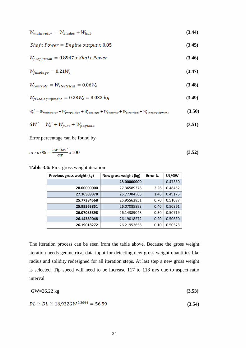
3.2. Gross weight iteration
An iteration of gross weight will be done by using statistical data [3]. The unit
conversion is done. This iteration process will go on until 5% error rate of gross
weight will be reached.
(3.42)
(3.43)
34
(3.44)
(3.45)
(3.46)
(3.47)
(3.48)
(3.49)
(3.50)
(3.51)
Error percentage can be found by
(3.52)
Table 3.6: First gross weight iteration
Previous gross weight (kg) New gross weight (kg) Error % UL/GW
28.00000000 0.47350
28.00000000 27.36589378 2.26 0.48452
27.36589378 25.77384568 1.46 0.49175
25.77384568 25.95563851 0.70 0.51087
25.95563851 26.07085898 0.40 0.50861
26.07085898 26.14389048 0.30 0.50719
26.14389048 26.19018272 0.20 0.50630
26.19018272 26.21952658 0.10 0.50573
The iteration process can be seen from the table above. Because the gross weight
iteration needs geometrical data input for detecting new gross weight quantities like
radius and solidity redesigned for all iteration steps. At last step a new gross weight
is selected. Tip speed will need to be increase 117 to 118 m/s due to aspect ratio
interval
GW=26.22 kg (3.53)
(3.54)

35
(3.55)
(3.56)
(3.57)
Maximum advance ratio and blade loading coefficient are;
(3.58)
(3.59)
(3.60)
(3.61)
Aspect ratio should be between 15 and 20. It is an acceptable value
(3.62)
(3.63)
As it was explained at the first iteration step, the average values of profile drag
coefficients will be used and for new design weight they need to determined again.
At hover the average drag coefficients of the stations located by 1 intervals at
sea level and 2000 meters altitude are 0.0096445 and 0.0092702 respectively.
These average values can be seen at the tables given below. At first, the local blade
station speeds are obtained in meters per second, then by using the speed of sound at
the defined altitudes local Mach numbers are obtained. With tables of airfoil, local
Reynolds numbers and corresponding local profile drag coefficients are defined. At
last average values of these coefficients are obtained.

36
Table 3.7: Determination of drag coefficient at blade stations at sea level
r Blade station speed (m/s) Mach number Reynolds number Profile Drag coefficient
0.2 23.4 0.068722467 96728.51296 0.014735835
0.3 35.1 0.1030837 145092.7694 0.012169134
0.4 46.8 0.137444934 193457.0259 0.010624013
0.4 46.8 0.137444934 193457.0259 0.010624013
0.5 58.5 0.171806167 241821.2824 0.009561963
0.6 70.2 0.206167401 290185.5389 0.008773513
0.7 81.9 0.240528634 338549.7954 0.00815783
0.8 93.6 0.274889868 386914.0518 0.007659536
0.9 105.3 0.309251101 435278.3083 0.007245335
1 117 0.343612335 483642.5648 0.006893835
Average 0.009644501
Table 3.8: Determination of drag coefficient at blade stations at 2000 meters
r Blade station speed (m/s) Mach number Reynolds number Profile Drag coefficient
0.2 23.4 0.069205626 105188.0424 0.014164079
0.3 35.1 0.103808439 157782.0636 0.011696967
0.4 46.8 0.138411252 210376.0849 0.010211797
0.4 46.8 0.138411252 210376.0849 0.010211797
0.5 58.5 0.173014065 262970.1061 0.009190956
0.6 70.2 0.207616878 315564.1273 0.008433097
0.7 81.9 0.242219691 368158.1485 0.007841303
0.8 93.6 0.276822504 420752.1697 0.007362343
0.9 105.3 0.311425316 473346.1909 0.006964213
1 117 0.346028129 525940.2122 0.006626352
Average 0.009270291
Table 3.9: Average profile drag coefficients
Profile drag coefficient
Sea level 0.0096445
2000 meters 0.0092702
At forward flight for all airspeeds independently, all stations profile drag coefficients
have been found and the average values of these values are stated at the table below.
At 2000 meters altitude all calculations were redone.
(3.64)

37
For this value of lift coefficent, mean angle of attack can be approximated as 4.5
degrees.
(3.65)
Lift curve slope can be calculated as;
(3.66)
(3.67)
Power required to hover OGE can be calculated as;
(3.68)
Root cut out ratio is 0.2 and induced power factor is 1.15
(3.69)
(3.70)
at sea level (3.71)
at sea level (3.72)
So the total power required to hover out-of-ground effect at sea level is;
(3.73)
Induced power is approximately 75% of total power.
The power required for rotor at hover at 2000 meters altitude is;
(3.74)
3.3. Power required to hover IGE
The profile does not change for hover IGE, but the induced power will be smaller. In
all cases ground effect will be negligible for rotors hovering greater than three rotor
radii above the ground [4].

38
Hayden assumed that only the induced part of the power is influenced by the
ground[4]. Assume that ground effect at 2 meters altitude will be calculated;
(3.75)
(3.76)
Where A= 0.9926 and B= 0.0379
(3.77)
(3.78)
Total power required to hover in-ground effect at two meters altitude is
which is smaller than power required to hover out-of-ground effect as
expected. It can be seen that above the altitude 3.6 meters there is no ground effect to
provide advantages to helicopter.
3.4. Power calculations at forward flight
For advancing ratios larger than 0.1, induced power for forward flight can be
approximated by Glauert high-speed formula which is given below; [4]
(3.79)
Because for high speeds, , thrust equation can be written as;
(3.80)
And the induced power is
Profile power for forward flight can be corrected with Stepniewski constant K=4.7
and it can be written as [4];
(3.81)
For climb speed occurance climb power can be defined as;

39
(3.82)
where is climb celocity and T is the thrust.
Parasitic power results from viscous shear effects and flow seperation on the
airframe,rotor hub and so on. Parasitic power can be calculated by equivalent flat
plate approach [4].
(3.83)
where f is equivalent flat plate area. This value can be calculated from helicopter data
history [3].
(3.84)
Here gross weight’s unit is kilogram and the exact formula from the reference shown
above was changed into SI unit system.
(3.85)
For example, with cruise level speed 80 km/h and 2000 meters altitude, the parasitic
power is expected to be lower.
(3.86)
For high speed forward flight, parasitic power will be larger than the lower speed
one.
Total main rotor power for forward flight will be calculated for two different
altitudes (sea level and 2000 meters) and for a speed range 0-130 km/h. Chord and
radius values will be fixed.
The calculator is constructed in Excel. The Matlab codes are not uısed at this stage.
Two different density of air values can be seen. The inputs and outputs can be seen
at the table given below.
40
Table 3.10: Forward flight power calculator
Gross weight 26.22 kg
Forward velocity in km/h INPUT
Forward velocity in m/s -------------------
Tip speed 117 m/s
Advance ratio -------------------
Density 1.225 or 1.0087 kg/m^3
Main rotor radius 1.202819122 m
Number of blades 2
Main rotor chord 0.060630997 m
Profile drag coefficient INPUT
Stepniewski constant 4.7
Equivalent flat plate area 0.033266803
Tip-loss effect 0.974796295
Root cut-out ratio 0.2
Effective rotor disk area 4.137143869
Induced power factor 1.15
Solidity 0.032090354
Profile power for hover OUTPUT (kW)
Profile power for forward flight OUTPUT (kW)
Induced power for hover OUTPUT (kW)
Induced power in forward flight for nu>0.1 OUTPUT (kW)
Parasitic power for forward flight OUTPUT (kW)
Total power for hover OUTPUT (kW)
Total power for forward flight OUTPUT (kW)
The important point in these calculations is remembering the induced power
approximation of Glauert is only valid when advance ratio is higher than 0.1. For the
speed values 10, 20, 30 and 40 km/h, the advance ratio is lower than 0.1; so
Glauert’s high-speed formula can not be used.
(3.87)
By using this equation ,for forward speeds less than 42.12 km/h for defined tip speed
117 m/s, a new approximation for induced power is required.
(3.88)
where induced velocity can be stated as; [4]

41
(3.89)
A numerical approach is required. Here induced velocity at hover is;
(3.90)
The error is acceptable and the convergence is said to occur if error rate which is
stated below is smaller than 0.0005.
(3.91)
These numerical approach can be approached by the Matlab code given above or by
using Excel.
Figure 3.9 : Matlab code for induced velocity iteration
For 10 km/h speed at sea level the tables of iteration are given to show the process,
for other speed values and altitude induced velocities are calculated and new forward
flight tables are constructed.

42
Table 3.11: Induced velocity iteration
v_i (m/s) v_i+1 (m/s)
0 9.135608661
2.601438526 6.42140156
3.5276232 5.447873909
4.023991762 5.009392535
4.28983731 4.796718253
4.429924769 4.690451048
4.502863435 4.636641925
4.540571423 4.609222682
4.559990113 4.595207292
4.569969685 4.588032117
4.575092844 4.584355882
4.577721432 4.582471585
4.579069721 4.581505567
4.579761202 4.58101027
4.580115806 4.580756306
4.580297647 4.580626083
4.580390893 4.580559308
4.580438708 4.580525068
4.580463227 4.58050751
4.5804758 4.580498507
4.580482247 4.580493891
4.580485553 4.580491523
4.580487248 4.580490309
4.580488117 4.580489687
4.580488563 4.580489368
4.580488791 4.580489204
4.580488909 4.58048912
4.580488969 4.580489077
4.580488999 4.580489055
4.580489015 4.580489044
4.580489023 4.580489038
4.580489028 4.580489035
4.58048903 4.580489033
4.580489031 4.580489033
4.580489031 4.580489032
4.580489032 4.580489032
4.580489032 4.580489032
4.580489032 4.580489032
4.580489032 4.580489032
4.580489032 4.580489032
4.580489032 4.580489032
4.580489032 4.580489032
4.580489032 4.580489032
4.580489032 4.580489032

43
Table 3.12 : Revised induced power values at sea level
Gross weight 26.22 26.22 26.22 26.22
Density(SEA LEVEL) 1.225 1.225 1.225 1.225
Radius 1.202819122 1.202819 1.202819 1.202819
Chord 0.060630997 0.060631 0.060631 0.060631
Root-cut out 0.2 0.2 0.2 0.2
Forward speed 2.778 5.556 8.334 11.112
Alfa(radian) 0.078539816 0.07854 0.07854 0.07854
Tip loss 0.974796295 0.974796 0.974796 0.974796
Effective disk area 4.137143867 4.137144 4.137144 4.137144
Thrust 257.2182 257.2182 257.2182 257.2182
Vh 5.037528236 5.037528 5.037528 5.037528
Forward speed km/h 10 20 30 40
Alfa(degrees) 4.5 4.5 4.5 4.5
Induced power factor 1.15 1.15 1.15 1.15
Obtained induced velocity 4.58048932 3.678179 2.818362 2.207275
Induced power at forward flight 1.354913001 1.088009 0.833674 0.652914
Table 3.13 : Revised induced power values 2000 meters
Gross weight 26.22 26.22 26.22 26.22
Density(2000 meters) 1.0087 1.0087 1.0087 1.0087
Radius 1.202819122 1.202819 1.202819 1.202819
Chord 0.060630997 0.060631 0.060631 0.060631
Root-cut out 0.2 0.2 0.2 0.2
Forward speed 2.778 5.556 8.334 11.112
Alfa(radian) 0.078539816 0.07854 0.07854 0.07854
Tip loss 0.974796295 0.974796 0.974796 0.974796
Effective disk area 4.137143867 4.137144 4.137144 4.137144
Thrust 257.2182 257.2182 257.2182 257.2182
Vh 5.551425645 5.551426 5.551426 5.551426
Forward speed km/h 10 20 30 40
Alfa(degrees) 4.5 4.5 4.5 4.5
Induced power factor 1.15 1.15 1.15 1.15
Obtained induced velocity 5.122765819 4.248555 3.342899 2.651348
Induced power at forward flight 1.515318893 1.256726 0.988832 0.784271

44
After the correction of induced power values below the advance ratio makes the
Glauert’s high speed formula wrong,new power tables can be revised. These revised
forward flight power tables can be written as;
Table 3.14: Power values at forward flight at sea level
Forward
Speed Profile Power Induced Power
Parasitic
Power
Total Power at
sea level
10 0.314852804 1.354913001 0.000436727 1.670202532
20 0.317348553 1.088008665 0.003493813 1.408851031
30 0.321508135 0.833674052 0.011791619 1.166973806
40 0.32733155 0.652914111 0.027950503 1.008196164
50 0.334818797 0.540464308 0.054590827 0.929873932
60 0.343969877 0.450386923 0.094332949 0.888689749
70 0.35478479 0.386045934 0.14979723 0.890627954
80 0.367263535 0.337790192 0.223604028 0.928657755
90 0.381406114 0.300257949 0.318373704 1.000037767
100 0.397212525 0.270232154 0.436726617 1.104171296
110 0.414682768 0.245665594 0.581283127 1.241631489
120 0.433816845 0.225193462 0.754663594 1.413673901
130 0.454614754 0.207870888 0.959488377 1.621974019
Table 3.15: Power values at forward flight at 2000 meters
Profile Power Induced Power
Parasitic
Power
Total Power at
2000m
10 0.249197043 1.515318893 0.000359613 1.764875549
20 0.251172357 1.256726392 0.002876905 1.510775654
30 0.254464548 0.988832494 0.009709556 1.253006598
40 0.259073615 0.784271087 0.023015243 1.066359945
50 0.264999558 0.656358458 0.044951647 0.966309663
60 0.272242378 0.546965382 0.077676446 0.896884206
70 0.280802074 0.46882747 0.123347319 0.872976863
80 0.290678646 0.410224036 0.184121945 0.885024627
90 0.301872095 0.364643588 0.262158004 0.928673687
100 0.31438242 0.328179229 0.359613174 1.002174823
110 0.328209621 0.298344754 0.478645135 1.10519951
120 0.343353699 0.273482691 0.621411565 1.238247955
130 0.359814652 0.252445561 0.790070144 1.402330357

45
The variation of powers at sea level with respect to increasing forward speed can be
seen at the figure below.
Figure 3.10 : Powers at forward flight at sea level
The tip Mach number of advancing side of the blade should also be checked.
(3.92)
Table 3.16: Tip mach number at sea level
Forward speed
km/h
Forward
speed m/s Tip Mach number
10 2.777777778 0.351770272
20 5.555555556 0.35992821
30 8.333333333 0.368086148
40 11.11111111 0.376244085
50 13.88888889 0.384402023
60 16.66666667 0.392559961
70 19.44444444 0.400717899
80 22.22222222 0.408875836
90 25.00000000 0.417033774
100 27.77777778 0.425191712
110 30.55555556 0.433349649
120 33.33333333 0.441507587
130 36.11111111 0.449665525
Tip speed 117 At sea level
Speed of
sound 340.5

46
Table 3.17: Tip mach number at 2000 meters
Forward speed
km/h
Forward speed
m/s Tip Mach number
10 2.777777778 0.354243422
20 5.555555556 0.362458715
30 8.333333333 0.370674008
40 11.11111111 0.3788893
50 13.88888889 0.387104593
60 16.66666667 0.395319886
70 19.44444444 0.403535178
80 22.22222222 0.411750471
90 25.00000000 0.419965764
100 27.77777778 0.428181057
110 30.55555556 0.436396349
120 33.33333333 0.444611642
130 36.11111111 0.452826935
Tip speed 117.0000000 At 2000 meters
Speed of sound 338.1228
All these power calculations are done considering a zero twist blade. At this work,
modified momentum theory is used for forward flight analysis and blade element
momentum theory approach will be used at the end of this chapter considering
twisted blades at hover. For the zero twist, results can be seen at the tables given
before and for twisted blades, results can be seen the table at the end of this chapter.
3.5. Twist rate calculation with BEMT
At this section an estimation of twist rate will be done. All other geometric
specifications of main rotor will be fixed.
Thrust coefficient taken from modified momentum theory will be used to determine
which twist rate should be used from BET analysis. The twist angle which has
obtained from BET, will be used in BEMT to determine inflow ratios and thrust
coefficients at the stations respectively.
For twist angles between zero and fifteen; twenty iterations has been made by the
formula given above [4].
(3.93)
is 8.033 /rad, solidity is 0.032090354. Tip loss factor is 0.974796295. Twist
angle values are given 0 to 15 and twenty iterations has been made in order to
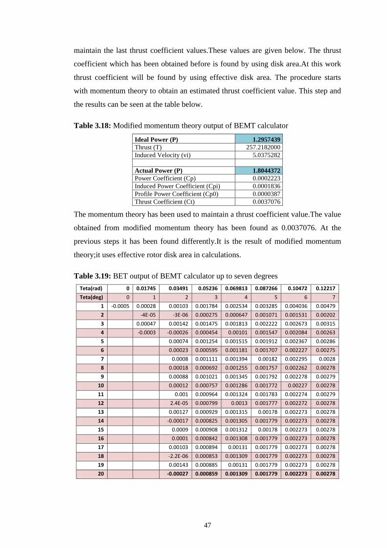
47
maintain the last thrust coefficient values.These values are given below. The thrust
coefficient which has been obtained before is found by using disk area.At this work
thrust coefficient will be found by using effective disk area. The procedure starts
with momentum theory to obtain an estimated thrust coefficient value. This step and
the results can be seen at the table below.
Table 3.18: Modified momentum theory output of BEMT calculator
Ideal Power (P) 1.2957439
Thrust (T) 257.2182000
Induced Velocity (vi) 5.0375282
Actual Power (P) 1.8044372
Power Coefficient (Cp) 0.0002223
Induced Power Coefficient (Cpi) 0.0001836
Profile Power Coefficient (Cp0) 0.0000387
Thrust Coefficient (Ct) 0.0037076
The momentum theory has been used to maintain a thrust coefficient value.The value
obtained from modified momentum theory has been found as 0.0037076. At the
previous steps it has been found differently.It is the result of modified momentum
theory;it uses effective rotor disk area in calculations.
Table 3.19: BET output of BEMT calculator up to seven degrees
Teta(rad) 0 0.01745 0.03491 0.05236 0.069813 0.087266 0.10472 0.12217
Teta(deg) 0 1 2 3 4 5 6 7
1 -0.0005 0.00028 0.00103 0.001784 0.002534 0.003285 0.004036 0.00479
2 -4E-05 -3E-06 0.000275 0.000647 0.001071 0.001531 0.00202
3 0.00047 0.00142 0.001475 0.001813 0.002222 0.002673 0.00315
4 -0.0003 -0.00026 0.000454 0.00101 0.001547 0.002084 0.00263
5 0.00074 0.001254 0.001515 0.001912 0.002367 0.00286
6 0.00023 0.000595 0.001181 0.001707 0.002227 0.00275
7 0.0008 0.001111 0.001394 0.00182 0.002295 0.0028
8 0.00018 0.000692 0.001255 0.001757 0.002262 0.00278
9 0.00088 0.001021 0.001345 0.001792 0.002278 0.00279
10 0.00012 0.000757 0.001286 0.001772 0.00227 0.00278
11 0.001 0.000964 0.001324 0.001783 0.002274 0.00279
12 2.4E-05 0.000799 0.0013 0.001777 0.002272 0.00278
13 0.00127 0.000929 0.001315 0.00178 0.002273 0.00278
14 -0.00017 0.000825 0.001305 0.001779 0.002273 0.00278
15 0.0009 0.000908 0.001312 0.00178 0.002273 0.00278
16 0.0001 0.000842 0.001308 0.001779 0.002273 0.00278
17 0.00103 0.000894 0.00131 0.001779 0.002273 0.00278
18 -2.2E-06 0.000853 0.001309 0.001779 0.002273 0.00278
19 0.00143 0.000885 0.00131 0.001779 0.002273 0.00278
20 -0.00027 0.000859 0.001309 0.001779 0.002273 0.00278

48
Table 3.20: BET output of BEMT calculator between 7 and 15 degrees twist angle
Teta(rad) 0,139626 0,15708 0,174533 0,191986 0,20944 0,226893 0,244346 0,261799
Teta(deg) 8 9 10 11 12 13 14 15
1 0,005537 0,006287 0,007038 0,007789 0,008539 0,00929 0,01004 0,010791
2 0,002523 0,003045 0,00358 0,004127 0,004683 0,005247 0,005819 0,006398
3 0,003654 0,004173 0,004706 0,00525 0,005805 0,006368 0,006939 0,007516
4 0,003176 0,003732 0,004296 0,004866 0,005442 0,006024 0,00661 0,007202
5 0,003368 0,003897 0,004439 0,004992 0,005555 0,006126 0,006704 0,007288
6 0,003289 0,003834 0,004388 0,00495 0,005519 0,006095 0,006677 0,007264
7 0,003321 0,003858 0,004406 0,004964 0,005531 0,006104 0,006685 0,007271
8 0,003308 0,003849 0,0044 0,00496 0,005527 0,006102 0,006682 0,007269
9 0,003313 0,003852 0,004402 0,004961 0,005528 0,006102 0,006683 0,007269
10 0,003311 0,003851 0,004401 0,004961 0,005528 0,006102 0,006683 0,007269
11 0,003312 0,003851 0,004401 0,004961 0,005528 0,006102 0,006683 0,007269
12 0,003312 0,003851 0,004401 0,004961 0,005528 0,006102 0,006683 0,007269
13 0,003312 0,003851 0,004401 0,004961 0,005528 0,006102 0,006683 0,007269
14 0,003312 0,003851 0,004401 0,004961 0,005528 0,006102 0,006683 0,007269
15 0,003312 0,003851 0,004401 0,004961 0,005528 0,006102 0,006683 0,007269
16 0,003312 0,003851 0,004401 0,004961 0,005528 0,006102 0,006683 0,007269
17 0,003312 0,003851 0,004401 0,004961 0,005528 0,006102 0,006683 0,007269
18 0,003312 0,003851 0,004401 0,004961 0,005528 0,006102 0,006683 0,007269
19 0,003312 0,003851 0,004401 0,004961 0,005528 0,006102 0,006683 0,007269
20 0,003312 0,003851 0,004401 0,004961 0,005528 0,006102 0,006683 0,007269
The thrust coefficient value obtained from modified momentum theory has been
found as 0.0037076. As it can be seen from the figure below, twist angle should be
8.8 degrees(actually by the figure below it is 8.8152 degrees,but it was approximated
to 8.8 degrees) .
Figure 3.11 : Variation of thrust coefficient with respect to twist angle

49
Power coefficient can be defined as the formula given below by the uniform inflow
and constant drag coefficient assumptions [4]
(3.94)
In hover with uniform inflow the equation given above, returns into simple
momentum theory because for this assumptions .So;
(3.95)
The second term is the extra power predicted by the BET that is required overcome
profile drag of blades, which has been already introduced in momentum theory.
So,the total power can be written as;
(3.96)
BET analysis will not be used at here to calculate total power. BEMT will be used by
using 40 stations at the blade. Firstly, inflow ratios at the stations will be calculated
and then, thrust and power coefficients will be found by using these inflow ratio
values. The estimated value for twist angle from BET will be used with a linear twist
distribution assumption.
Blade element momentum theory was used for power calculations for twisted blades.
The inflow ratio on each station can be found by; [4]
(3.97)
Where n=(1,N) element station number, and are the radius and pitch angle
at the mid-span of each of the N stations. Here, N equals to 40. Thrust coefficients
can be calculated and summed by rectangular approach.
(3.98)
(3.99)
The 8.8 twist angle is used in calculations.

50
The tables of this process can be seen from the table for sea level computations
below.
Table 3.21: Input of BEMT
Seçilen twist 8.8
Effective AoA 4.4
Delta r 0.0225
Table 3.22: Output of BEMT
Section Inflow ratio Ct Cpi
0,10000000 0,00000 0,00000000000 0,00000000000
0,11125000 0,01171 0,00000137329 0,00000003217
0,13375000 0,01340 0,00000216138 0,00000005792
0,15625000 0,01496 0,00000314606 0,00000009411
0,17875000 0,01640 0,00000432832 0,00000014199
0,20125000 0,01775 0,00000570686 0,00000020260
0,22375000 0,01901 0,00000727862 0,00000027676
0,24625000 0,02020 0,00000903921 0,00000036510
0,26875000 0,02131 0,00001098319 0,00000046809
0,29125000 0,02236 0,00001310427 0,00000058600
0,31375000 0,02335 0,00001539543 0,00000071896
0,33625000 0,02429 0,00001784912 0,00000086697
0,35875000 0,02517 0,00002045726 0,00000102987
0,38125000 0,02601 0,00002321140 0,00000120741
0,40375000 0,02680 0,00002610269 0,00000139920
0,42625000 0,02755 0,00002912203 0,00000160476
0,44875000 0,02826 0,00003226004 0,00000182349
0,47125000 0,02893 0,00003550711 0,00000205474
0,49375000 0,02957 0,00003885344 0,00000229773
0,51625000 0,03017 0,00004228908 0,00000255165
0,53875000 0,03074 0,00004580391 0,00000281559
0,56125000 0,03127 0,00004938769 0,00000308858
0,58375000 0,03177 0,00005303008 0,00000336960
0,60625000 0,03224 0,00005672064 0,00000365759
0,62875000 0,03268 0,00006044884 0,00000395141
0,65125000 0,03310 0,00006420410 0,00000424990
0,67375000 0,03348 0,00006797577 0,00000455188
0,69625000 0,03384 0,00007175316 0,00000485610
0,71875000 0,03417 0,00007552554 0,00000516132
0,74125000 0,03447 0,00007928217 0,00000546625
0,76375000 0,03475 0,00008301227 0,00000576961
0,78625000 0,03500 0,00008670505 0,00000607009
0,80875000 0,03523 0,00009034975 0,00000636637
0,83125000 0,03543 0,00009393559 0,00000665715
0,85375000 0,03561 0,00009745180 0,00000694110
0,87625000 0,03577 0,00010088766 0,00000721692
0,89875000 0,03590 0,00010423245 0,00000748331
0,92125000 0,03600 0,00010747551 0,00000773899
0,94375000 0,03609 0,00011060623 0,00000798270
0,96625000 0,03615 0,00011361403 0,00000821319
0,98875000 0,03618 0,00011648843 0,00000842926

51
The thrust coefficients at each station is summed and the obtained result is
0.00206705945. The induced power coefficients are also summed up and profile
power coefficient is obtained with the values of profile drag coefficient and solidity.
These two power coefficient is summed and total power coefficient is obtained.This
coefficient is used to obtain total power value at hover by BEMT. The total out of
ground effect power at hover obtained by BEMT at sea level and 2000 meters
altitude can be stated as;
Table 3.23: Total power with BEMT
Sea level 2000 meters
Total Power 1.432984 kW 1.565378 kW
When the values for 2000 meters altitude were obtained, the twist angle founded
from BET was changed. The value was 10.1 degree approximately. It means at that
altitude, the value of required thrust can only be obtained by equal or higher values
of twist.This means for a fixed twist more power is needed.
BET can be used to determine at what rate should the blades have and can be used to
estimate how much power needed during the hover mission. The modified
momentum theory is nearly have the same error rates with BEMT but the momentum
theory does not contain the inflow on the blades,twist rates,etc.
Main rotor calculations is completed and the tail rotor design with respect to these
power requirements will be done at Chapter 4. These values which were used here
should not be written as with too mant unnecessary decimals, but these values used
here are calculated using Microsoft Excel and nothing was changed. The Excel
format and Matlab code of design uses same decimal values.
At the end of this chapter, the values calculated here, namely the new concept,
should be shown in one table.
At cruise speed 80 km/h, helicopter’s some specifications can be summarized as

52
Table 3.24: Helicopter's specifications
Gross weight 26.22 kg
Required cruise speed 80 km/h
Maximum Forward speed 130 km/h
Blade tip speed 117 m/s
Thrust coeeficient 0.003374764
Solidity 0.032090354
Maximum advance ratio 0.308641
Mean lift coefficient 0.630986557
Airfoil Boeing-Vertol VR7
Main rotor radius 1.202819122 m
Chord 0.060690997
Blade twist 8.8 degrees
Airfoil lift-curve slope 8.033 /rad
Airfoil profile drag coefficient 0.014683642 at sea level
Number of blades 2
Aspect ratio of main rotor 19.93
Induced power at hover 1.490105537 kW
Profile power at hover 0.311020886 kW
Total power OGE at hover 1.804126422kW
Total power IGE at hover 1.7367 kW for 2 meters
Power at hover with twisted blades 1.432984 kW
Induced power at forward flight (80km/h) 0.337790192 kW
Profile power at forward flight(80km/h) 0.3672635 kW
Parasitic power at forward flight(80km/h) 0.223604028 kW
Total power at forward flight(80km/h) 0.928657 kW

53
4. TAIL ROTOR DESIGN
Tail rotor provides an anti-torque force to encounter the torque of the main rotor on
the airframe. It also gives yaw stability and makes the control of aircraft on the yaw
axis desirable. Another advantage of tail rotor its weathercock stability [4]. For
example if the aircraft is yawed nose-left ,then the tail rotor will experince an
additional climb performance.
4.1. Preliminary tail rotor geometry
Radius of the tail rotor is roughly one sixth of the radius of the main rotor and the tip
speed of tail rotor is approximately is the same as the main rotor tip speed which
means the rotational velocities of the tail rotors are roughly six times of the main
rotor rotational velocity which is an important issue needs to be solved for rotor
noise levels problems [4]. For small helicopters, the ratio of the radius of the main
rotor and tail rotor can be approximated as six, but with increasing gross weight this
ratio will be much more smaller than that [3]. At this work, the ratio will be accepted
as six and the tip speed of the tail rotor approximated as 117 m/s. NACA 0012
airfoil will be used for tail rotor blades.
(4.1)
(4.2)
(4.3)
This RPM value is too high, but decreasing the tip speed gives increase in power
needs of the tail rotor. The airfoil is used for main rotor is different so the drag
coefficient of the tail rotor can be stated as 0.011 for NACA 0012 for hovering
performance [12]. As it was mentioned at Chapter 2 in trade studies, the number of
blades of the tail rotor is 2.

54
The distance from the main rotor shaft and the tail rotor shaft can be approximated
as;
(4.4)
These 0.2 value is an approximation and it is defined as 0.5 ft in English unit system
[3].
The aspect ratios for tail rotors can be changed between 4.5 and 8 [5]. By the
definition an approximated chord value can be obtained for an aspect ratio as 6.
(4.5)
4.2. Power required
Power needed for tail rotor at hover will be much more than power needed at forward
flight. But at high forward speeds,the power sometimes can exceed the hovering
value.
4.2.1. Power required at hover
The thrust needed for tail rotor can be stated as;
(4.6)
And the thrust coefficient can be found by;
(4.7)
Tip-loss factor B will be calculated with;
(4.8)
or tip-loss factor can be stated with thrust coefficient as;
(4.9)
The induced and profile powers for tail rotor can be stated as;
(4.10)

55
(4.11)
(4.12)
The power values for the hovering can be seen from the table above. The profile drag
coefficient is assumed to be constant as NACA 0012 airfoil is used for tail rotor zero
twisted blades.
Table 4.1: Tail rotor power for untwisted main rotor blades at sea level
Main rotor total power at sea level 1.800496029 kW
Main rotor rotational velocity 97.27148318 rad/s
Distance between main and tail rotor shafts 1.603288976 m
Thrust required at tail rotor at hover 11.54502356 N
Thrust coefficient of tail rotor at hover 0.005453044
Tip-loss factor 0.947783892
Density 1.225
Radius of main rotor 1.202819122 m
Radius of tail rotor 0.200469854 m
Disk area of tail rotor 0.126254835
Aspect ratio of tail rotor 6
Chord of tail rotor 0.033411642 m
Solidity of tail rotor 0.106060606
Profile drag coefficient of main rotor 0.0096445
Profile drag coefficient of tail rotor 0.011
Tip speed of tail rotor 117 m/s
Number of blades of tail rotor 2
Induced power at hover for tail rotor 74.41763431 W
Profile power at hover for tail rotor 36.12422146 W
Total power at hover OGE for tail rotor 110.5418558 W
Total power required of tail rotor at hover OGE at sea level is 0.110 kW.Another
table needs to be constructed for 2000 meters altitude. It is already founded that total
hovering power for 2000 meters is 1.89 kW for untwisted blades.
For 2000 meters altitude the table will be reconstructed and it can be seen at below.
But these values are calculated for untwisted main rotor blades.

56
Table 4.2: Tail rotor power for untwisted main rotor blades at 2000 meters
Main rotor total power at 2000 meters 1.890655471 kW
Main rotor rotational velocity 97.27148318 rad/s
Distance between main and tail rotor shafts 1.603288976 m
Thrust required at tail rotor at hover 12.12313807 N
Thrust coefficient of tail rotor at hover 0.00695118
Tip-loss factor 0.941045866
Density 1.0087
Radius of main rotor 1.202819122 m
Radius of tail rotor 0.200469854 m
Disk area of tail rotor 0.126305653
Aspect ratio of tail rotor 6
Chord of tail rotor 0.033411642 m
Solidity of tail rotor 0.106060606
Profile drag coefficient of main rotor 0.0092702
Profile drag coefficient of tail rotor 0.011
Tip speed of tail rotor 117 m/s
Number of blades of tail rotor 2
Induced power at hover for tail rotor 88.85960612 W
Profile power at hover for tail rotor 29.7576887 W
Total power at hover OGE for tail rotor 118.6172948 W
For twisted main rotor blades, the power required for main rotor is obtained as
P=1.80 kW for sea level and P=1.89 kW for 2000 meters altitude.
For linearly twisted main rotor blades with a twist angle 8.8 degrees, the tables need
to be reconstructed and the power requirements for the tail rotor need to be
recalculated. Results can be seen from the tables below.
As twist of main rotor has been taken into account, the power needs of main rotor
decreased. As it is expected, the tail rotor power needed for encountering the torque
produced by main rotor was also decreased.
These power values considering twisted main rotor blades will be used during the
design.

57
Table 4.3: Tail rotor power for twisted main rotor blades at sea level
Main rotor total power at sea level with twisted blades 1.432984 kW
Main rotor rotational velocity 97.27148318 rad/s
Distance between main and tail rotor shafts 1.603288976 m
Thrust required at tail rotor at hover 9.188486825 N
Thrust coefficient of tail rotor at hover 0.004338238
Tip-loss factor 0.953426197
Density 1.225
Radius of main rotor 1.202819122 m
Radius of tail rotor 0.200469854 m
Disk area of tail rotor 0.126305653
Aspect ratio of tail rotor 6
Chord of tail rotor 0.033411642 m
Solidity of tail rotor 0.106060606
Profile drag coefficient of main rotor 0.0096445
Profile drag coefficient of tail rotor 0.011
Tip speed of tail rotor 117 m/s
Number of blades of tail rotor 2
Induced power at hover for tail rotor 52.51513409 W
Profile power at hover for tail rotor 36.13876144 W
Total power at hover OGE for tail rotor 88.65389552 W
Table 4.4: Tail rotor power for twisted main rotor blades at 2000 meters
Main rotor total power at 2000 meters with twisted blades 1.565378 kW
Main rotor rotational velocity 97.27148318 rad/s
Distance between main and tail rotor shafts 1.603288976 m
Thrust required at tail rotor at hover 10.03741502 N
Thrust coefficient of tail rotor at hover 0.005755265
Tip-loss factor 0.946356429
Density 1.0087
Radius of main rotor 1.202819122 m
Radius of tail rotor 0.200469854 m
Disk area of tail rotor 0.126305653
Aspect ratio of tail rotor 6
Chord of tail rotor 0.033411642 m
Solidity of tail rotor 0.106060606
Profile drag coefficient of main rotor 0.0092702
Profile drag coefficient of tail rotor 0.011
Tip speed of tail rotor 117 m/s
Number of blades of tail rotor 2
Induced power at hover for tail rotor 66.56879311 W
Profile power at hover for tail rotor 29.7576887 W
Total power at hover OGE for tail rotor 96.32648181 W

58
4.2.2. Power required at forward flight
Power required at forward flight for both main and tail rotors will be smaller than the
hovering rotors. This makes the hovering performance the key point at design
process. Tail rotor power will be calculated for different forward flight speeds and of
course because of the changing profile drag coefficients, the tail rotor’s performance
is affected.
(4.13)
where at forward flight, total power which is the sum of profile,parasitic and induced
power was calculated before for different airspeeds. These data will be used for
obtaining the required thrust for tail rotor. Then; thrust coefficient,tip-loss factor and
induced power are obtained for different advance ratios.The data at sea level can be
seen the table below.
Table 4.5: Tail rotor power at forward flight at sea level
Forward
speed
Total power
of main rotor at forward
flight
Thrust
required at tail
rotor to encounter
torque
Thrust
coefficient
Tip-loss
factor Profile power
Induced
power
Tail rotor power at sea
level
10 1.670202532 10.70956407 0.005058433 0.949708686 36.21992315 66.35294879 102.5728719
20 1.408851031 9.033742971 0.004266894 0.953810746 36.50702824 51.18377716 87.6908054
30 1.166973806 7.482793556 0.003534337 0.957962298 36.98553671 38.41847983 75.40401654
40 1.008196164 6.464689882 0.003053457 0.960926624 37.65544857 30.75560439 68.41105296
50 0.929873932 5.962477161 0.002816248 0.962475022 38.51676383 27.19841358 65.71517741
60 0.888689749 5.698398621 0.002691516 0.963315424 39.56948247 25.38947223 64.9589547
70 0.890627954 5.710826652 0.002697386 0.963275442 40.8136045 25.47363526 66.28723976
80 0.928657755 5.954678872 0.002812565 0.962499569 42.24912993 27.14437977 69.39350969
90 1.000037767 6.412377139 0.003028749 0.961085038 43.87605874 30.37803777 74.25409651
100 1.104171296 7.080095383 0.003344131 0.959109103 45.69439094 35.31698314 81.01137408
110 1.241631489 7.961508699 0.003760448 0.956638452 47.70412653 42.22193915 89.92606568
120 1.413673901 9.064667863 0.004281501 0.953731754 49.90526551 51.45108638 101.3563519
130 1.621974019 10.40031634 0.004912366 0.950440107 52.29780788 63.45093368 115.7487416
As it can be seen from the tables, at very low or very high airpeeds the power
required to transmitted to tail rotor is exceeds the hovering value. Profile drag
coefficient is assumed to be constant for tail rotor calculations and the expression
which gives the induced part of the total power at forward flight is constructed to
obtain a thrust to encounter the main rotor torque.

59
For 2000 meters altitude,the forward flight performance of tail rotor is;
Table 4.6: Tail rotor power at forward flight at 2000 meters
Forward
speed
Total power of main rotor
at forward
flight
Thrust
required at tail rotor to
encounter
torque
Thrust
coefficient
Tip-loss
factor Profile power
Induced
power
Tail rotor
power at
2000m
10 1.764875549 11.31662023 0.006488738 0.943040639 29.83652393 79.97187938 109.8084033
20 1.510775654 9.687297411 0.005554514 0.947300311 30.07302962 63.05345201 93.12648163
30 1.253006598 8.03444743 0.004606801 0.952006244 30.46720576 47.39001232 77.85721807
40 1.066359945 6.837643899 0.003920577 0.955724857 31.01905235 37.06119644 68.08024879
50 0.966309663 6.196107989 0.003552732 0.957853043 31.72856941 31.89864109 63.6272105
60 0.896884206 5.750942586 0.003297483 0.959395305 32.59575692 28.47761124 61.07336816
70 0.872976863 5.597645476 0.003209585 0.95994014 33.62061489 27.33106341 60.9516783
80 0.885024627 5.674897367 0.00325388 0.959664658 34.80314331 27.90680476 62.70994807
90 0.928673687 5.954781029 0.00341436 0.958681967 36.14334219 30.02733116 66.17067335
100 1.002174823 6.426080233 0.003684594 0.957078014 37.64121152 33.71820709 71.35941861
110 1.105199510 7.086688433 0.004063374 0.954925761 39.29675132 39.13704195 78.43379326
120 1.238247955 7.939813018 0.00455254 0.95228973 41.10996157 46.54134284 87.6513044
130 1.402330357 8.991931532 0.005155805 0.949226952 43.08084227 56.27325334 99.35409561

60

61
5. TOTAL POWER CALCULATIONS AND ENGINE SELECTION
5.1. Total power calculations
At this section, total power required for hover and forward flight will be determined,
required rotor shaft power will be determined at sea level and operational altitude
and at the end engine shaft power will be determined.
5.1.1. Total power required for hover and forward flight
Total power required for hover is the sum of total main rotor power and total tail
rotor power at hover for specified design. The design and all power values will
change at the selection of motor at Chapter 5.2. So, all of the calculations at Chapter
3, Chapter 4 and Chapter 5.1 will be recalculated.
Total power for hover can be stated as;
(5.1)
At sea level and the operational altitude 2000 meters the total power required for
hover for the design with zero-twisted main rotor blades and with twisted main rotor
blades can be seen at the table below.
Table 5.1: Total power at hover
Main rotor
power for
hover OGE
Tail rotor
power for
hover OGE
Total power
for hover
OGE
Zero-twisted main rotor blades at sea level 1.804126 kW 0.110541 kW 1.914667 kW
Zero-twisted main rotor blades at 2000 m 1.890655 kW 0.118617 kW 2.009272 kW
Twisted main rotor blades at sea level 1.432984 kW 0.087919 kW 1.520903 kW
Twisted main rotor blades at 2000 m 1.565378 kW 0.096326 kW 1.661704 kW
Total power for forward flight is the sum of main rotor and tail rotor powers at
specified speed values.It can be stated as;
(5.2)

62
All these values can be seen the tables which are constructed for both sea level and
2000 meters are given below.
Table 5.2: Total power at forward flight at sea level
Forward speed Main rotor power Tail rotor power Total power at sea level (kW)
10 1.670202532 0.102572872 1.772775404
20 1.408851031 0.087690805 1.496541836
30 1.166973806 0.075404017 1.242377822
40 1.008196164 0.068411053 1.076607216
50 0.929873932 0.065715177 0.995589109
60 0.888689749 0.064958955 0.953648704
70 0.890627954 0.06628724 0.956915193
80 0.928657755 0.06939351 0.998051265
90 1.000037767 0.074254097 1.074291863
100 1.104171296 0.081011374 1.185182670
110 1.241631489 0.089926066 1.331557555
120 1.413673901 0.101356352 1.515030253
130 1.621974019 0.115748742 1.737722761
Table 5.3: Total power at forward flight at 2000 meters
Forward speed Main rotor power Tail rotor power Total power at 2000 m (kW)
10 1.764875549 0.109808403 1.874683952
20 1.510775654 0.093126482 1.603902136
30 1.253006598 0.077857218 1.330863816
40 1.066359945 0.068080249 1.134440194
50 0.966309663 0.06362721 1.029936874
60 0.896884206 0.061073368 0.957957574
70 0.872976863 0.060951678 0.933928541
80 0.885024627 0.062709948 0.947734575
90 0.928673687 0.066170673 0.994844360
100 1.002174823 0.071359419 1.073534241
110 1.10519951 0.078433793 1.183633303
120 1.238247955 0.087651304 1.325899259
130 1.402330357 0.099354096 1.501684453

63
5.1.2. Required shaft power
The power required will be selected as the maximum power at forward flight at 2000
meters altitude namely 1.874683952 kW. Power values for hover are higher than that
value but the zero twisted condition has not taken into acccount because the blades
have twist.
Table 5.4: Comparison of power values
Maximum Power at forward flight
Power at hover with zero twist
Power at hover with twist
At sea level 1.772775404 kW 1.914667 kW 1.520903 kW
At 2000 meters 1.874683952 kW 2.009272 kW 1.661704 kW
Power needs of helicopter can be seen from the table above. The biggest value of
power at both sea level and operational altitude forward flight power tables is the
value given above.From now on, zero twisted main rotor configuration is not
considered. Therefore, required rotor shaft power can be stated as the maximum
power at the table namely 1.874683952 kW
5.1.3. Required total engine shaft power
Required total engine shaft power can be calculated by considering fifteen percent of
transmission and accessories losses [3]. So,the required total engine shaft power can
be stated as;
(5.3)
5.2. Engine selection
Total required engine power was approximated. At here, an engine, which is capable
of encountering the power requirements of the helicopter, will be selected here. At
first engine’s type will be selected. In general, two stroke engines have an excellent
power-to-weight ratio and are relatively inexpensive. They are unfortunately also not
very fuel efficient and exhibit high vibration and noise levels. Four cylinder engines
are the most fuel efficient internal combustion engines. They however have lower
vibration and noise levels than the two stroke engines, but have a higher vibration
level than a Wankel engine. They also have a lower power-to-weight ratio than a two
stroke engine of comparable power output.

64
A figure shows the displacement required at the 4 stroke engine for the required
power.
Figure 5.1 : Power output with respect to displacement for 4 stroke engines [13]
By using the formula given at the figure above, the displacement required at a 4-
stroke engine can be stated as; [13]
(5.4)
A 30cc engine will works for the design. Capacities for the given engines at the table
are calculated by using the formulas which are given below; [13]
(5.5)
(5.6)
J/ccfam is an efficiency unit.It means energy in joules per cc of fuel air mixture.
At the table given below specifications of some engines are shown. These values are
obtained from different sources. [13]
A wankel engine is selected. Because it produces less noise compared with 2 stroke
and 4 stroke engines. The selected engine is NR 20 EH 36 cc, four stroke, petrol
(gasoline) engine. Some detailed specifications for the selected engine are given at
the Table 5.6. The required engine shaft power 2.195 kW.

65
Table 5.5: Engine database
Engine Manufacturer Type
Mass
(kg)
Power
output (kW)
Efficiency
(J/ccfam)
Capacity
(cc)
BGX-1
3500 RN O.S. Engines
2-stroke methanol
powered 1.34
3.06 kW at
10,000 rpm 0.525 35
116 Gx 2 Evolution Engines
2-stroke gasoline
powered 1.493
3.015 kW at
8,500 rpm 0.615 34
G450PU Zenoah(Husqvarna)
2-stroke pre-mixed
fuel powered 2.148
2.9 kW at
8000 rpm 0.483 45
FT-300 O.S. Engines
2-cylinder 4-stroke
glow fuel powered 1.828
3.0 kW at
7,000 rpm 1.05 50
FF-300
radial O.S. Engines
5 cylinder 4-stroke
glow fuel powered 2.673
3.0 kW at
8,000 rpm 0.905 50
FF-320 O.S. Engines
4 cylinder 4-stroke
glow fuel powered 2.19
3.06 kWat
8,000 rpm 0.846 55
FA-300T Saito Engines
2 cylinder 4-stroke
glow fuel powered 1.75
3.504 kW at
8000 rpm 1.168 45
FA-300TD Saito Engines
2 cylinder 4-stroke
glow fuel powered 1.85
3.579 kW at
8000 rpm 1.136 45
Kavan Kavan
4 stroke petrol
powered 2.6
3.28 kW at
9200 rpm 0.856 50
FG-36 Saito Engines
36 cc, four stroke,
petrol (gasoline)
engine 1.76
2.6 kW at
8300 rpm 1.164 36
Sonic 30 Cubewano Wankel 1.5
3.72 kW at
8000 rpm
Wren 44
Heli engine Wren Turbines Gas turbine engine 5.2
5.1 kW at
15000 rpm
NRG 20EH Nitto
Wankel 20cc
Gasoline powered 1.8 1.34 kW
NR 20EH Nitto
Wankel 20cc
Alcohol powered 1.493 2.24 kW
Wren heli
engine Wren Turbines Gas turbine engine 2.077
6 kW at
13500 rpm
Raket 120 Raket 6.8
10 kW at
9000 rpm
37SZ-H
Ringed heli
engine O.S. Engines 0.293
1.03 kW at
18000 rpm 6.07
50SX-H
Ringed
Hyper Heli
Engine O.S. Engines 0.406
1.42 kW at
17000 rpm 8.17
55HZ-H
Hyper
Ringed Heli
engine O.S. Engines 0.408
1.57 kW at
17000 rpm 8.93
70SZ-H
Ring 3D
Heli Engine O.S. Engines 0.553
1.86 kW at
16000 rpm 11.5
91HZ
Ringed Heli
engine O.S. Engines 0.618
2.74 kW at
15000 rpm 14.95
Speed
Tuned
91HZ-R 3C
Heli engine O.S. Engines 0.603
2.98 kW at
15500 rpm 14.9

66
Figure 5.2 : Nitto NR 20 EH Wankel engine
Figure 5.3 : Draftings of selected engine [14]
Table 5.6: Specifications of selected engine [14]
Weight 1.493 kg
Displacement 20cc
Fuel type Glow(Alcohol)
Fuel consumption 38cc/min
Power 2.24 kW at 9500
RPM
RPM Range 2000-13000
Maximum operational altitude 4000 m

67
6. DESIGN FOR SELECTED ENGINE
6.1. Main rotor design
For the selected engine a new gross weight iteration has to be done because
estimated fuel weight and engine weight is decreased. The engine’s fuel consumption
is 38cc/min. Density of alcohol is approximately 790 [15]
The new fuel weight for the defined mission time equals to one hour is;
(6.1)
Engine’s weight is 1.493 kg.
So; gross weight iteration can be defined as;
(6.2)
(6.3)
(6.4)
(6.5)
(6.6)
(6.7)
(6.8)
At this step of design,it is assumed that transmission losses are 15%, which was
assumed that 10% at the premature steps of the design. This gives a more reliable
design.
(6.9)

68
(6.10)
(6.11)
(6.12)
(6.13)
(6.14)
(6.15)
Using the formulas given above a new gross weight value is obtained and by using
the formulas given below a new design is completed.By using the values of this new
design, another gross weight value is obtained. Aimed error rate between gross
weight is 10%.
(6.16)
(6.17)
(6.18)
(6.19)
Advance ratio and blade loading coefficient are;
(6.20)
(6.21)
(6.22)
During the design iteration, it has been taken into account that the aspect ratio should
be between the interval 15 and 20. When it is more than 20, tip speed is decreased.
(6.23)
For new aspect ratio chord can be stated as;

69
(6.24)
By using blade loading, mean lift coefficient can be expressed as;
(6.25)
The input of for first iteration of gross weight can be seen the table below.
Table 6.1: Geometric specifications of design before last iteration
Gross weight 26.22
Disk loading 56.59149598
Radius 1.202819122
Tip speed 117
Density 1.2250
Area 4.545174068
Maximum forward speed 130
Number of blades 2
Thrust coeff. 0.003374764
Max. advance ratio 0.308641975
Blade loading 0.105164426
Solidity 0.032090354
Aspect ratio 19.83835315
Chord 0.060630997
After the first iteration new gross weight value can be seen the table below. This
procedure will go on until error rate will be under 10% percentage.
Table 6.2: Weight of design
Payload weight 9.54
Fuel weight 1.8
Empty weight 14.88
Engine weight 1.493
Engine output 2.24
Shaft power 1.904
Propulsion weight 1.703509
Fuselage weight 3.1248
Controls 0.8928
Electrical 0.8928
Fixed eq 4.1664
Blades 0.20599
Hub 0.131358
New gross weight 22.45766

70
During the gross weight iteration these error percentages and gross weight values are
obtained;
Table 6.3: New gross weight iteration
Iteration number
Previous gross weight
New gross weight Error % UL/GW
1 26.62 23.70828309 10.93808 0.478314
2 23.70828309 21.85938739 7.798522 0.51877
3 21.85938739 20.68668018 5.364776 0.548179
The iteration process is terminated because the useful load per gross weight ratio can
not exceed 0.55.A new gross weight value should be selected.
New gross weight is 20.68668018 kg. For this gross weight geometric specification
of the main rotor can be seen at the table below.
Table 6.4: Last geometric specifications of design
Gross weight 20.68668018
Disk loading 51.84709662
Radius 1.116201873
Tip speed 113
Density 1.2250
Area 3.914131086
Maximum forward speed 130
Number of blades 2
Thrust coeff. 0.003314603
Max. advance ratio 0.319567355
Blade loading 0.103728026
Solidity 0.031954745
Aspect ratio 19.92254287
Chord 0.056027078
The aspect ratio should be between 15 and 20. Therefore tip speed was decreased.
(6.26)
For this value of lift coefficient, mean angle of attack can be approximated as 4.3
degrees.
(6.27)
Lift curve slope can be calculated as;

71
(6.28)
(6.29)
Profile drag coefficient can be calculated at
To obtain profile drag coefficient values, the assumptions at Chapter 3 should be
remade. At this chapter not only the average values will be shown; all tables used in
obtaining the average profile drag coefficients will be given step by step.
At hover the profile drag coefficients at sea level and 2000 meters altitude at the
blade stations can be seen at the tables given below.
Table 6.5: Profile drag coefficients at blade stations at hover at sea level
r Speed at station Mach number Reynolds number
Profile Drag
coefficients at sea level
0.2 22.6 0.066372981 86371.89378 0.015544927
0.3 33.9 0.099559471 129557.8407 0.012837298
0.4 45.2 0.132745962 172743.7876 0.01120734
0.4 45.2 0.132745962 172743.7876 0.01120734
0.5 56.5 0.165932452 215929.7344 0.010086976
0.6 67.8 0.199118943 259115.6813 0.009255235
0.7 79.1 0.232305433 302301.6282 0.008605747
0.8 90.4 0.265491924 345487.5751 0.008080093
0.9 101.7 0.298678414 388673.522 0.00764315
1 113 0.331864905 431859.4689 0.007272351
The average value of the profile drag coefficients at sea level is obtained from the
table as 0.010174046.
Table 6.6: Profile drag coefficients at blade stations at hover at 2000 meters
r Speed at station Mach number Reynolds number
Profile Drag coefficients
at 2000 meters
0.2 22.6 0.06684 93925.67 0.014942
0.3 33.9 0.100259 140888.5 0.012339
0.4 45.2 0.133679 187851.3 0.010772
0.4 45.2 0.133679 187851.3 0.010772
0.5 56.5 0.167099 234814.2 0.009696
0.6 67.8 0.200519 281777 0.008896
0.7 79.1 0.233939 328739.8 0.008272
0.8 90.4 0.267358 375702.7 0.007767
0.9 101.7 0.300778 422665.5 0.007347
1 113 0.334198 469628.4 0.00699

72
The average value of the profile drag coefficients at 2000 meters altitude is obtained
from the table as 0.009779.The variation of drag coefficient values with respect to
location on the blade can be seen at the figure given below.
Table 6.7: Mean profile drag coefficients
Mean profile drag coefficients
at hover
Sea level 0.010174046
2000 meters 0.009779289
Figure 6.1: Profile drag coefficient change with respect to blade station
Power required to hover OGE can be calculated as;
(6.30)
Root cut out ratio is 0.2 and induced power factor is 1.15
(6.31)
(6.32)
at sea level (6.33)
at sea level (6.34)

73
So the total power required to hover out-of-ground effect at sea level is;
(6.35)
For fixed geometric design parameters,the total power required to hover out-of
ground effect at 2000 meters is;
(6.36)
Power required to hover IGE can be found by;
Assume that ground effect at 2 meters altitude will be calculated;
(6.37)
(6.38)
where A= 0.9926 and B= 0.0379
(6.39)
(6.40)
Twist rate can be calculated by BEMT. Input of BEMT can be seen the table below.
Blade element theory is used for calculating the twist by comparing the thrust
coefficient value obtained from classical momentum theory. By considering the twist
value obtained from blade element momentum theory, inflow ratios, thrust
coefficients, power coefficients and power values are obtained at each station with
blade element momentum theory. All of these values are summed and total power
required value is obtained for blades with defined twist rates. Twist is used at blades
to decrease the power requirements of design.
Because of necessary twist, modified momentum theory can not be used. Blade
element theory and blade element momentum theory was used for obtaining twist
and the new power requirements.

74
Table 6.8: Input of BEMT
Max. Take-off Weight (W) 20.68668018
Gravitational Constant (g) 9.81
Air Density (ρ_SL) 1.225
Air Density (ρ_2000) 1.0087
Effective Disc Area (Ae) 3.563563793
Disc Area (A) 3.914131088
Pi (π) 3.141592654
Rotor Diameter (D) 2.232403746
Rotor Radius ( R) 1.1162018730
Number of Blades (Nb) 2
Chord ( c) 0.056027078
Solidity (ς) 0.031954744
Cd0 0.010174046
Kapha (к) 1.15
Blade Tip Velocity (Vtip) 113
Rotor RPM 966.7341905
Rotor Root Cutout 0.2
Radial Velocity (Ω) 101.2361677
Clα 8.2827
Tip loss factor 0.974902802
Power output of engine 2.24 kW
The pre-work with momentum theory has already be done for hover,but it can be
seen the table below. At the table, ideal power means the power without tip losses
and without root cut-out losses. It is the result of momentum theory, but the actual
power is the result of modified momentum theory. The power required is increased
by considering the losses with modified theory.
Table 6.9: Modified momentum theory output of BEMT calculator
Ideal Power (P) 0.9783954
Thrust (T) 202.9363326
Induced Velocity (vi) 4.8211938
Actual Power (P) 1.3811282
Power Coefficient (Cp) 0.0002193
Induced Power Coefficient (Cpi) 0.0001786
Profile Power Coefficient (Cp0) 0.0000406
Thrust Coefficient (Ct) 0.0036407
The momentum theory has been used to maintain a thrust coefficient value.The value
obtained from modified momentum theory has been found as 0.0036407. At the
previous steps it has been found differently.It is the result of modified momentum
theory; it uses effective rotor disk area in calculations.

75
Table 6.10: BET output of calculator up to seven degrees
Teta(rad) 0 0.017453 0.034907 0.05236 0.069813 0.087266 0.10472 0.122173
Teta(deg) 0 1 2 3 4 5 6 7
1 -0.00048 0.00029 0.00106 0.00183 0.0026 0.00337 0.004139 0.004909
2 -4.7E-05 -2.3E-05 0.000257 0.000633 0.001064 0.001532 0.002027
3 0.00044 0.001312 0.001541 0.001873 0.002284 0.002741 0.003229
4 -0.00024 -0.0002 0.000426 0.001003 0.001556 0.002107 0.002662
5 0.000864 0.001319 0.00156 0.001957 0.002417 0.002913
6 0.000129 0.000567 0.001184 0.001727 0.00226 0.002799
7 0.000995 0.001167 0.001428 0.001855 0.002338 0.00285
8 2.63E-05 0.00067 0.001266 0.001782 0.002299 0.002827
9 0.001294 0.001067 0.001372 0.001823 0.002318 0.002838
10 -0.00019 0.000742 0.001302 0.0018 0.002309 0.002833
11 0.000884 0.001003 0.001348 0.001813 0.002313 0.002835
12 0.000113 0.00079 0.001318 0.001806 0.002311 0.002834
13 0.001031 0.000961 0.001338 0.00181 0.002312 0.002834
14 -8.6E-07 0.000822 0.001324 0.001808 0.002312 0.002834
15 0.001495 0.000934 0.001333 0.001809 0.002312 0.002834
16 -0.00032 0.000843 0.001327 0.001808 0.002312 0.002834
17 0.000687 0.000916 0.001331 0.001809 0.002312 0.002834
18 0.000282 0.000857 0.001329 0.001808 0.002312 0.002834
19 0.000734 0.000905 0.00133 0.001809 0.002312 0.002834
20 0.00024 0.000866 0.001329 0.001809 0.002312 0.002834
Table 6.11: BET output of calculator between 8 and 15 degrees
Teta(rad) 0.139626 0.15708 0.174533 0.191986 0.20944 0.226893 0.244346 0.261799
Teta(deg) 8 9 10 11 12 13 14 15
1 0.005679 0.006449 0.007219 0.007989 0.008759 0.009529 0.010299 0.011069
2 0.002542 0.003075 0.003621 0.004179 0.004747 0.005324 0.005908 0.006499
3 0.003739 0.004268 0.004811 0.005366 0.005932 0.006507 0.00709 0.007679
4 0.003224 0.003794 0.00437 0.004953 0.005542 0.006137 0.006738 0.007343
5 0.003434 0.003973 0.004526 0.005091 0.005666 0.006249 0.006839 0.007436
6 0.003347 0.003904 0.00447 0.005044 0.005626 0.006215 0.00681 0.00741
7 0.003383 0.00393 0.00449 0.00506 0.005639 0.006225 0.006818 0.007417
8 0.003368 0.00392 0.004483 0.005055 0.005635 0.006222 0.006816 0.007415
9 0.003374 0.003924 0.004486 0.005057 0.005636 0.006223 0.006816 0.007416
10 0.003371 0.003923 0.004485 0.005056 0.005636 0.006223 0.006816 0.007416
11 0.003373 0.003923 0.004485 0.005056 0.005636 0.006223 0.006816 0.007416
12 0.003372 0.003923 0.004485 0.005056 0.005636 0.006223 0.006816 0.007416
13 0.003372 0.003923 0.004485 0.005056 0.005636 0.006223 0.006816 0.007416
14 0.003372 0.003923 0.004485 0.005056 0.005636 0.006223 0.006816 0.007416
15 0.003372 0.003923 0.004485 0.005056 0.005636 0.006223 0.006816 0.007416
16 0.003372 0.003923 0.004485 0.005056 0.005636 0.006223 0.006816 0.007416
17 0.003372 0.003923 0.004485 0.005056 0.005636 0.006223 0.006816 0.007416
18 0.003372 0.003923 0.004485 0.005056 0.005636 0.006223 0.006816 0.007416
19 0.003372 0.003923 0.004485 0.005056 0.005636 0.006223 0.006816 0.007416
20 0.003372 0.003923 0.004485 0.005056 0.005636 0.006223 0.006816 0.007416

76
The thrust coefficient value obtained from modified momentum theory has been
found as 0.0036407. As it can be seen from the figure below, twist angle should be
8.3 degrees(actually by the figure below it is 8.32388 degrees,but it was
approximated to 8.3 degrees) .
Figure 6.2 : Thrust coefficient twist angle change of last design
Power coefficient can be defined as the formula given below by the uniform inflow
and constant drag coefficient assumptions
(6.41)
In hover with uniform inflow the equation given above, returns into simple
momentum theory because for this assumptions .So;
(6.42)
The second term is the extra power predicted by the BET that is required overcome
profile drag of blades, which has been already introduced in momentum theory.
So,the total power can be written as;
(6.43)
BET analysis will not be used at here to calculate total power. BEMT will be used by
using 40 stations at the blade. Firstly, inflow ratios at the stations will be calculated
and then, thrust and power coefficients will be found by using these inflow ratio

77
values. The estimated value for twist angle from BET will be used with a linear twist
distribution assumption.
Blade element momentum theory was used for power calculations for twisted blades.
The inflow ratio on each station can be found by;
(6.44)
where n=(1,N) element station number, and are the radius and pitch angle
at the mid-span of each of the N stations. Here, N equals to 40. Thrust coefficients
can be calculated and summed by rectangular approach.
(6.45)
(6.46)
The 8.8 twist angle is used in calculations. The tables of this process can be seen
from the table for sea level computations below.
Table 6.12: Input for BEMT for last design
Seçilen twist 8.3
Effective AoA 4.3
Delta r 0.0225
The thrust coefficients at each station is summed and the obtained result is
0.00201402625. The induced power coefficients is also summed up and profile
power coefficient is obtained with the values of profile drag coefficient and solidity.
These two power coefficient is summed and total power coefficient is obtained.This
coefficient is used to obtain total power value at hover by BEMT. The total out of
ground effect power at hover obtained by BEMT at sea level and 2000 meters
altitude can be stated at Table 6.14

78
Table 6.13: Output of BEMT for last design
Section Inflow ratio Ct Cpi
0.10000000 0.00000 0.00000000000 0.00000000000
0.11125000 0.01135 0.00000129092 0.00000002932
0.13375000 0.01301 0.00000203753 0.00000005302
0.15625000 0.01454 0.00000297301 0.00000008646
0.17875000 0.01596 0.00000409894 0.00000013086
0.20125000 0.01729 0.00000541465 0.00000018724
0.22375000 0.01853 0.00000691772 0.00000025643
0.24625000 0.01970 0.00000860442 0.00000033908
0.26875000 0.02081 0.00001046998 0.00000043567
0.29125000 0.02185 0.00001250876 0.00000054651
0.31375000 0.02283 0.00001471443 0.00000067179
0.33625000 0.02376 0.00001708007 0.00000081154
0.35875000 0.02464 0.00001959829 0.00000096570
0.38125000 0.02547 0.00002226129 0.00000113404
0.40375000 0.02626 0.00002506089 0.00000131628
0.42625000 0.02701 0.00002798863 0.00000151199
0.44875000 0.02772 0.00003103579 0.00000172068
0.47125000 0.02839 0.00003419342 0.00000194177
0.49375000 0.02903 0.00003745237 0.00000217457
0.51625000 0.02963 0.00004080332 0.00000241837
0.53875000 0.03020 0.00004423679 0.00000267233
0.56125000 0.03074 0.00004774319 0.00000293561
0.58375000 0.03125 0.00005131280 0.00000320726
0.60625000 0.03173 0.00005493581 0.00000348631
0.62875000 0.03218 0.00005860233 0.00000377174
0.65125000 0.03260 0.00006230239 0.00000406249
0.67375000 0.03300 0.00006602595 0.00000435744
0.69625000 0.03337 0.00006976295 0.00000465547
0.71875000 0.03371 0.00007350325 0.00000495541
0.74125000 0.03403 0.00007723670 0.00000525608
0.76375000 0.03432 0.00008095313 0.00000555627
0.78625000 0.03459 0.00008464235 0.00000585477
0.80875000 0.03483 0.00008829416 0.00000615035
0.83125000 0.03505 0.00009189836 0.00000644176
0.85375000 0.03524 0.00009544475 0.00000672777
0.87625000 0.03542 0.00009892316 0.00000700715
0.89875000 0.03557 0.00010232344 0.00000727867
0.92125000 0.03569 0.00010563546 0.00000754110
0.94375000 0.03580 0.00010884913 0.00000779323
0.96625000 0.03588 0.00011195440 0.00000803389
0.98875000 0.03594 0.00011494129 0.00000826189
Table 6.14: Power values of BEMT for last design
Sea level 2000 meters
Total Power 1.0920618 kW 1.156943 kW

79
When the values for 2000 meters altitude were obtained the twist angle founded from
BET was changed. The value was 9.8 degree approximately.(Actual value is 9.75164
degrees) It means at that altitude, the value of required thrust can only be obtained by
equal or higher values of twist.This means for the designed twist, helicopter needs
more power; more twist. This power difference is easily be encountered because the
helicopter actually needs more power from that value at relatively high speeds.
Induced power for forward flight will be calculated for 0 to 40 km/h forward speeds
by classical formula with numerical iteration for induced velocity and 40 to 130 km/h
by Glauert’s high-speed formula. Profile power is found with the help of Stepniewski
constant and parasitic power will be calculated with equivalent flat plate approach.
(6.47)
This is the Glauert’s high-speed formula’s necessity.Forward speeds less than 11.5
m/s (40.68 km/h)must be considered with classical induced power formula with
numerical approach to induced velocity.
The input table for the speeds higher than 40 km/h can be at Table 6.15
Total main rotor power for forward flight will be calculated for two different
altitudes (sea level and 2000 meters) and for a speed range 0-130 km/h. Chord and
radius values will be fixed.
The calculator is constructed in Excel. The Matlab codes are not uısed at this stage.
Two different density of air values can be seen. The inputs and outputs can be seen
at the table given below.

80
Table 6.15: Forward flight power calculator for last design
Gross weight 20.68668018
Forward velocity in km/h INPUT
Forward velocity in m/s ----------------------
Tip speed 113
Advance ratio ----------------------
Density 1.225 or 1.0087
Main rotor radius 1.116201873
Number of blades 2
Main rotor chord 0.056027078
Profile drag coefficient INPUT
Stepniewski constant 4.7
Equivalent flat plate area 0.02728868
Tip-loss effect 0.9749028
Root cut-out ratio 0.2
Effective rotor disk area 3.5635637
Induced power factor 1.15
Solidity 0.03195474
Profile power for hover OUTPUT
Profile power for forward flight OUTPUT
Induced power for hover OUTPUT
Induced power in forward flight (50-130
km/h) OUTPUT
Parasitic power for forward flight OUTPUT
Total power for hover OUTPUT
Total power for forward flight OUTPUT
And the input of numerical approach to induced velocity to obtain induced power
between forward speeds 0 and 40 km/h can be stated as;
Table 6.16: Induced power calculator for advance ratios smaller than 0.1
Gross weight 20.68668018
Density 1.225 or 1.0087
Radius 1.116201873
Chord 0.056027078
Root-cut out 0.2
Forward speed Conversion of speed to m/s
Alfa(radian) 0.075049158
Tip loss 0.9749028
Effective disk area 3.5635637
Thrust 202.9363325
Vh Depends on density
Forward speed km/h INPUT(0 to 40 km/h)
Alfa(degrees) 4,3
Induced power factor 1,15
Obtained induced velocity Comes from numerical
analysis
Induced power at forward flight OUTPUT

81
The induced velocities obtained during numerical approach can be seen at the table
below for the changing forward speeds.
Table 6.17: Obtained induced velocities for last design
Forward
Speed(km/h)
Induced velocity at sea
level(m/s)
Induced velocity at
2000 meters(m/s)
10 4.354574572 4.875685391
20 3.442709119 3.988335955
30 2.60693535 3.09981241
40 2.031091019 2.443140059
50 1.647522832 1.991004187
60 1.38136929 1.672808113
70 1.187769475 1.439843648
80 1.041186444 1.26287055
90 0.926550835 1.124211775
100 0.834527345 1.012779361
110 0.759063495 0.921333734
120 0.696076769 0.844970744
130 0.642718715 0.780259238
Induced velocity in m/s change with respect to forward velocity in km/h can be seen
at the figure below.
Figure 6.3: Induced velocity variation with respect to forward speed
By using these inputs, the power tables of different velocities at sea level and 2000
meters altitude can be stated as;

82
Table 6.18: Power values at forward flight at sea level
Forward Speed Profile Power Induced Power Parasitic Power Total Power
10 0.2567005 1.016256603 0.000358246 1.273315348
20 0.258881483 0.803448377 0.002865967 1.065195827
30 0.262516454 0.608398184 0.009672637 0.880587275
40 0.267605414 0.474009487 0.022927732 0.764542633
50 0.274148362 0.390570403 0.044780727 0.709499492
60 0.282145299 0.325475336 0.077381096 0.685001731
70 0.291596224 0.278978859 0.122878315 0.693453398
80 0.302501138 0.244106502 0.183421858 0.730029498
90 0.314860041 0.216983557 0.2611612 0.793004798
100 0.328672932 0.195285202 0.358245816 0.882203949
110 0.343939812 0.177532001 0.47682518 0.998296993
120 0.36066068 0.162737668 0.619048769 1.142447117
130 0.378835536 0.150219386 0.787066057 1.316120979
Table 6.19: Power values at forward flight at 2000 meters
Profile Power Induced Power Parasitic Power Total Power
10 0.203173111 1.137871769 0.00029499 1.341339869
20 0.204899313 0.930785012 0.002359919 1.138044244
30 0.207776318 0.723424246 0.007964726 0.93916529
40 0.211804124 0.570172166 0.01887935 0.800855639
50 0.216982731 0.474322141 0.03687373 0.728178602
60 0.223312141 0.395268451 0.063717805 0.682298397
70 0.230792352 0.338801529 0.101181515 0.670775396
80 0.239423364 0.296451338 0.151034798 0.686909501
90 0.249205179 0.263512301 0.215047593 0.727765073
100 0.260137795 0.237161071 0.29498984 0.792288706
110 0.272221213 0.215600973 0.392631477 0.880453663
120 0.285455433 0.197634225 0.509742444 0.992832102
130 0.299840454 0.182431593 0.648092679 1.130364725
Glauert’s high speed formula gives 0.278978859332098 kW induced power for 70
km/h at sea level. The induced velocity at 70 km/h at sea level is 1.18776947545784
m/s. With the induced velocity which is obtained from numerical approach, the
induced power is 0.277197818475472 kW. By these data the error percentage of
Glauert high-speed formula can be stated as approximately 6%.
The variation of powers for changing forward velocity at sea level and 2000 meters
and the total power curves of these two altitudes can be seen the figures given below.

83
Figure 6.4 : Power versus forward speed at sea level
Figure 6.5 : : Power versus forwrad speed at 2000 meters
Figure 6.6 : Comparison of total power values obtained at different altitudes

84
The tip Mach number of the advancing side of the blade is checked.
Table 6.20: Tip mach number for last design
Forward speed
km/h
Forward speed
m/s
Tip Mach
number
10 2.777777778 0.340022842
20 5.555555556 0.348180780
30 8.333333333 0.356338718
40 11.11111111 0.364496655
50 13.88888889 0.372654593
60 16.66666667 0.380812531
70 19.44444444 0.388970468
80 22.22222222 0.397128406
90 25.00000000 0.405286344
100 27.77777778 0.413444281
110 30.55555556 0.421602219
120 33.33333333 0.429760157
130 36.11111111 0.437918094
Tip speed 113
Speed of sound 340.5
At specified cruise speed 80 km/h some specifications of main rotor can summarized
as;
Table 6.21: Specifications of last design
Gross weight 20.686680182973 m
Cruise speed 80 km/h
Maximum Forward speed 130 km/h
Blade tip speed 113 m/s
Thrust coefficient 0.00331460259294509
Solidity 0.0319547447622814
Maximum advance ratio 0.319567354965585
Mean lift coefficient 0.622368155515528
Airfoil Boeing-Vertol VR7
Main rotor radius 1.11620187258989 m
Chord 0.0560270784696832 m
Blade twist 8.3 degrees
Airfoil lift-curve slope 8.2827 /rad
Airfoil profile drag coefficient(sea level) 0.010174045641733
Number of blades 2
Aspect ratio of main rotor 1,9922542868157500
Induced power at hover 1.12515470625714 kW
Profile power at hover 0.255973507368591 kW
Total power OGE at hover 1.38112821362573 kW
Total power IGE at hover 1.33804 kW for 2 meters
Power at hover with twisted blades 1.0920618 kW
Induced power at forward flight(80 km/h) 0.244106502 kW
Profile power at forward flight(80km/h) 0.302501 kW
Parasitic power at forward flight(80 km/h) 0.183421858 kW
Total power at 80km/h 0.730029 kW

85
6.2. Tail rotor design
Radius of the tail rotor is roughly one sixth of the radius of the main rotor and the tip
speed of tail rotor is approximately is the same as the main rotor tip speed. For small
helicopters, the ratio of the radius of the main rotor and tail rotor can be
approximated as six, but with increasing gross weight, this ratio will be much more
smaller than that. At this work, the ratio will be accepted as six and the tip speed of
the tail rotor approximated as 113 m/s. NACA 0012 airfoil will be used for tail rotor
blades.
(6.48)
(6.49)
The airfoil is used for main rotor is different so the drag coefficient of the tail rotor
can be stated as 0.011 for NACA 0012. As it was mentioned at Chapter 2 in trade
studies, the number of blades of the tail rotor is 2. The distance from the main rotor
shaft and the tail rotor shaft can be approximated as;
(6.50)
The aspect ratios for tail rotors can be changed between 4.5 and 8. [5] By the
definition an approximated chord value can be obtained for an aspect ratio as 6.
(6.51)
Power needed for tail rotor at hover will be much more than power needed at forward
flight. But at high forward speeds, the power sometimes can exceed the hovering
value.
The thrust needed for tail rotor can be stated as;
(6.52)
And the thrust coefficient can be found by;
(6.53)

86
Tip-loss factor B will be calculated with;
(6.54)
or tip-loss factor can be stated with thrust coefficient as;
(6.55)
The induced and profile powers for tail rotor can be stated as;
(6.56)
(6.57)
(6.58)
The power values for the hovering can be seen from the tables above. The profile
drag coefficient is assumed to be constant as NACA 0012 airfoil is used for tail rotor
zero twisted blades. There are four tables located below which two are constructed
for two different altitudes,namely sea level and 2000 meters and the other two
constructed for illustrating zero-twisted main rotor blades or twisted main rotor
blades conditions.
The weight approximations can not be used for unmanned helicopters, these
approximations are given for example. Tail rotor power values also depends on these
calculations, so the values calculated here are not correct actually.
Hovering performance is the key point at design process because power required at
forward flight for both main and tail rotors will be smaller than the hovering rotors
except high forward speeds. Tail rotor power will be calculated for different forward
flight speeds and of course because of the changing profile drag coefficients, the tail
rotor’s performance is affected.
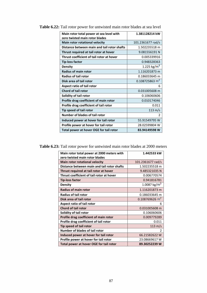
87
Table 6.22: Tail rotor power for untwisted main rotor blades at sea level
Main rotor total power at sea level with zero twisted main rotor blades
1.381128214 kW
Main rotor rotational velocity 101.2361677 rad/s
Distance between main and tail rotor shafts 1.502235518 m
Thrust required at tail rotor at hover 9.081556191 N
Thrust coefficient of tail rotor at hover 0.005339916
Tip-loss factor 0.948328363
Density 1.225 kg/
Radius of main rotor 1.116201873 m
Radius of tail rotor 0.186033645 m
Disk area of tail rotor 0.108725863
Aspect ratio of tail rotor 6
Chord of tail rotor 0.031005608 m
Solidity of tail rotor 0.106060606
Profile drag coefficient of main rotor 0.010174046
Profile drag coefficient of tail rotor 0.011
Tip speed of tail rotor 113 m/s
Number of blades of tail rotor 2
Induced power at hover for tail rotor 55.91549795 W
Profile power at hover for tail rotor 28.02599804 W
Total power at hover OGE for tail rotor 83.94149598 W
Table 6.23: Tail rotor power for untwisted main rotor blades at 2000 meters
Main rotor total power at 2000 meters with zero twisted main rotor blades
1.442533 kW
Main rotor rotational velocity 101.2361677 rad/s
Distance between main and tail rotor shafts 1.502235518 m
Thrust required at tail rotor at hover 9.485321035 N
Thrust coefficient of tail rotor at hover 0.006770574
Tip-loss factor 0.941816781
Density 1.0087 kg/
Radius of main rotor 1.116201873 m
Radius of tail rotor 0.186033645 m
Disk area of tail rotor 0.108769626
Aspect ratio of tail rotor 6
Chord of tail rotor 0.031005608 m
Solidity of tail rotor 0.106060606
Profile drag coefficient of main rotor 0.009779289
Profile drag coefficient of tail rotor 0.011
Tip speed of tail rotor 113 m/s
Number of blades of tail rotor 2
Induced power at hover for tail rotor 66.21582622 W
Profile power at hover for tail rotor 23.08669617 W
Total power at hover OGE for tail rotor 89.30252239 W

88
Table 6.24: Tail rotor power for twisted main rotor blades at sea level
Main rotor total power at sea level with twisted main rotor blades
1.0920618 kW
Main rotor rotational velocity 101.2361677 rad/s
Distance between main and tail rotor shafts
1.502235518 m
Thrust required at tail rotor at hover 7.18081095 N
Thrust coefficient of tail rotor at hover 0.004220587
Tip-loss factor 0.954062068
Density 1.225 kg/
Radius of main rotor 1.116201873 m
Radius of tail rotor 0.186033645 m
Disk area of tail rotor 0.108769626
Aspect ratio of tail rotor 6
Chord of tail rotor 0.031005608 m
Solidity of tail rotor 0.106060606
Profile drag coefficient of main rotor 0.010174046
Profile drag coefficient of tail rotor 0.011
Tip speed of tail rotor 113 m/s
Number of blades of tail rotor 2
Induced power at hover for tail rotor 39.07030051 W
Profile power at hover for tail rotor 28.03727849 W
Total power at hover OGE for tail rotor 67.107579 W
Table 6.25: Tail rotor power for twisted main rotor blades at 2000 meters
Main rotor total power at 2000 meters with twisted main rotor blades
1.156943 kW
Main rotor rotational velocity 101.2361677 rad/s
Distance between main and tail rotor shafts
1.502235518 m
Thrust required at tail rotor at hover 7.60743482 N
Thrust coefficient of tail rotor at hover 0.005430148
Tip-loss factor 0.947893626
Density 1.0087 kg/
Radius of main rotor 1.116201873 m
Radius of tail rotor 0.186033645 m
Disk area of tail rotor 0.108769626
Aspect ratio of tail rotor 6
Chord of tail rotor 0.031005608 m
Solidity of tail rotor 0.106060606
Profile drag coefficient of main rotor 0.009779289
Profile drag coefficient of tail rotor 0.011
Tip speed of tail rotor 113 m/s
Number of blades of tail rotor 2
Induced power at hover for tail rotor 47.25501791 W
Profile power at hover for tail rotor 23.08669617 W
Total power at hover OGE for tail rotor 70.34171408 W

89
(6.59)
where at forward flight, total power which is the sum of profile, parasitic and
induced power was calculated before for different airspeeds. These data will be used
for obtaining the required thrust for tail rotor. Then thrust coefficient,tip-loss factor
and induced power are obtained for different advance ratios.The data at sea level can
be seen the table below.
Table 6.26: Tail rotor power at forward flight at sea level
Forward
speed Total Power
Thrust required
at tail rotor to
encounter torque
Thrust
coefficient
Tip-loss
factor
Profile
power
Induced
power
Tail rotor
power
10 1.273315348 8.372636783 0.004923075 0.950386118 28.1056 49.39054 77.49614004
20 1.065195827 7.004154761 0.004118413 0.95462152 28.34439 37.62296 65.96734147
30 0.880587275 5.790268231 0.003404653 0.958740741 28.74237 28.15771 56.90008386
40 0.764542633 5.027221086 0.002955984 0.961555336 29.29955 22.71267 52.01222263
50 0.709499492 4.665287003 0.002743169 0.962965092 30.01592 20.27484 50.29076909
60 0.685001731 4.504202904 0.002648452 0.963610084 30.89149 19.22101 50.11249813
70 0.693453398 4.559776523 0.002681129 0.96338628 31.92625 19.58238 51.50863116
80 0.730029498 4.800281281 0.002822545 0.962433094 33.12021 21.17288 54.29309366
90 0.793004798 5.214372974 0.003066029 0.960846271 34.47336 24.01042 58.48378019
100 0.882203949 5.80089861 0.003410904 0.958702884 35.9857 28.23641 64.22210964
110 0.998296993 6.564264021 0.003859759 0.956069606 37.65724 34.08318 71.74042028
120 1.142447117 7.512117691 0.004417093 0.953004825 39.48798 41.85998 81.34795394
130 1.316120979 8.654103584 0.005088576 0.949559065 41.4779 51.94714 93.42504598
Table 6.27: Tail rotor power at forward flight at 2000 meters
Forward
speed Total Power
Thrust required at tail rotor to
encounter torque
Thrust
coefficient
Tip-loss
factor
Profile
power
Induced
power
Tail rotor
power
10 1.341339869 8.819929442 0.00629562 0.943894649 23.15226505 59.24126416 82.3935292
20 1.138044244 7.48316677 0.00534145 0.948320959 23.34897169 46.08111318 69.43008487
30 0.939165290 6.175445745 0.004408 0.953053212 23.67681608 34.37442891 58.05124498
40 0.800855639 5.265995885 0.00375884 0.956647715 24.13579823 26.96614773 51.10194596
50 0.728178602 4.788110784 0.00341773 0.958661584 24.72591814 23.33088085 48.05679899
60 0.682298397 4.486427234 0.00320239 0.959985071 25.4471758 21.13180711 46.57898292
70 0.670775396 4.410658179 0.00314831 0.960324406 26.29957123 20.59146809 46.89103931
80 0.686909501 4.516747372 0.00322403 0.959850085 27.28310441 21.34938987 48.63249428
90 0.727765073 4.785391638 0.00341579 0.958673324 28.39777535 23.31072396 51.70849931
100 0.792288706 5.209664338 0.00371863 0.956880213 29.64358404 26.52816525 56.1717493
110 0.880453663 5.789389674 0.00413244 0.954544324 31.0205305 31.153242 62.1737725
120 0.992832102 6.528329833 0.00465989 0.951730503 32.52861471 37.41444599 69.9430607
130 1.130364725 7.432670384 0.0053054 0.948495619 34.16783667 45.6070683 79.77490497

90
As it can be seen from the tables, at very low or very high airpeeds the power
required to transmitted to tail rotor is exceeds the hovering value. Profile drag
coefficient is assumed to be constant for tail rotor calculations and the expression
which gives the induced part of the total power at forward flight is constructed to
obtain a thrust to encounter the main rotor torque.
6.3. Total power calculations
Total power for hover can be stated as;
(6.60)
At sea level and the operational altitude 2000 meters the total power required for
hover for the design with zero-twisted main rotor blades and with twisted main rotor
blades can be seen at the table below.
Table 6.28: Total power at hover
Main rotor power for hover OGE
Tail rotor power for hover OGE
Total power for hover OGE
Zero-twisted main rotor blades at sea level 1.381128 kW 0.0839414 kW 1.465069 kW
Zero-twisted main rotor blades at 2000 m 1.442533 kW 0.0893025 kW 1.531835 kW
Twisted main rotor blades at sea level 1.0920618 kW 0.067107 kW 1.159169 kW
Twisted main rotor blades at 2000 m 1.156943 kW 0.070341 kW 1.2272847 kW
Total power for forward flight is the sum of main rotor and tail rotor powers at
specified speed values.It can be stated as;
(6.61)
All these values can be seen the tables which are constructed for both sea level and
2000 meters are given at Table 6.29 and Table 6.30. As it can be seen from the tables
with the increasing altitude, power requirements of helicopter durng forward flight
decreases. This happens because of decreasing air drag force with increasing
altiude,therefore decreasing parasitic drag.
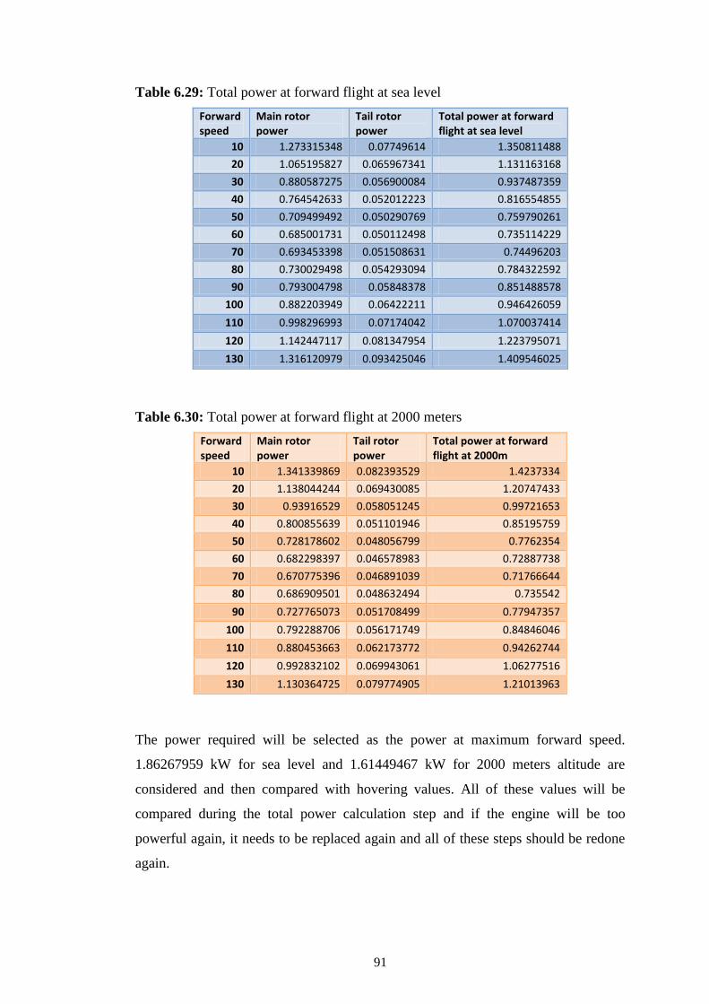
91
Table 6.29: Total power at forward flight at sea level
Forward speed
Main rotor power
Tail rotor power
Total power at forward flight at sea level
10 1.273315348 0.07749614 1.350811488
20 1.065195827 0.065967341 1.131163168
30 0.880587275 0.056900084 0.937487359
40 0.764542633 0.052012223 0.816554855
50 0.709499492 0.050290769 0.759790261
60 0.685001731 0.050112498 0.735114229
70 0.693453398 0.051508631 0.74496203
80 0.730029498 0.054293094 0.784322592
90 0.793004798 0.05848378 0.851488578
100 0.882203949 0.06422211 0.946426059
110 0.998296993 0.07174042 1.070037414
120 1.142447117 0.081347954 1.223795071
130 1.316120979 0.093425046 1.409546025
Table 6.30: Total power at forward flight at 2000 meters
Forward speed
Main rotor power
Tail rotor power
Total power at forward flight at 2000m
10 1.341339869 0.082393529 1.4237334
20 1.138044244 0.069430085 1.20747433
30 0.93916529 0.058051245 0.99721653
40 0.800855639 0.051101946 0.85195759
50 0.728178602 0.048056799 0.7762354
60 0.682298397 0.046578983 0.72887738
70 0.670775396 0.046891039 0.71766644
80 0.686909501 0.048632494 0.735542
90 0.727765073 0.051708499 0.77947357
100 0.792288706 0.056171749 0.84846046
110 0.880453663 0.062173772 0.94262744
120 0.992832102 0.069943061 1.06277516
130 1.130364725 0.079774905 1.21013963
The power required will be selected as the power at maximum forward speed.
1.86267959 kW for sea level and 1.61449467 kW for 2000 meters altitude are
considered and then compared with hovering values. All of these values will be
compared during the total power calculation step and if the engine will be too
powerful again, it needs to be replaced again and all of these steps should be redone
again.

92
Table 6.31: Comparison of power values for new design
Maximum power at forward flight
Power at hover with zero twist
Power at hover with twist
At sea level 1.409546025 kW 1.465069 kW 1.159169 kW
At 2000 meters 1.4237334 kW 1.531835 kW 1.2272847 kW
Power needs of helicopter can be seen from the table above. The biggest value of
power at both sea level and operational altitude forward flight power tables is the
value given above. Required rotor shaft power can be stated as the maximum power
at the table namely 1.4237334 kW. The zero twisted conditions are not taken into
account.
Required total engine shaft power can be calculated by considering fifteen percent of
transmission and accessories losses. Maximum engine power output is 2.24 kW.
So,the required total engine shaft power can be stated as;
(6.62)
A safety factor should be taken into account as 1.2 to overcome the instability
conditions, other environmental effects and inaccuracy rate of momentum theory,
modified momentum theory, BET and BEMT [16]. The rotor shaft power with
respect to these statements can be defined as;
(6.63)
So the engine is said to be suitable for the new design. The difference between the
available and the required shaft powers are considered in determining the climb
performance at Chapter 7.

93
7. PERFORMANCE ANALYSIS
7.1. Effect of density altitude
Two different altitudes was considered at this work;sea level and 2000 meters. With
the increasing altitude, the power required is expected to increase in hover and lower
airspeeds but at higher airspeeds with increasing altitude the power required is
expected to decrease because of the lower density results lower parasitic drag. Higher
density altitude actually affects the engine’s performance but it has not been taken
into account here because of the decreasing power requirements of helicopter with
increasing altitude value.
Figure 7.1: Power curves due to forward speed and different altitudes
These statements can be seen from the figure above. At 2000 meters at higher
airspeed less power is required by rotors compared with sea level but at low
airspeeds at 2000 meters higher power is required by rotors than the sea level.
7.2. Lift-to-Drag Ratios
The lift-to-drag ratio of the rotor alone is; [4]
(7.1)

94
The lift-to-drag ratio of the complete helicopter can be stated as;
(7.2)
Figure 7.2: Lift to drag ratios of design
L/D increases raipdly as induced power requirements decrease and reaches a
maximum,then drops off as the parasitic power requirements rapidly increase.
The values that is plotted at the figure above can be seen at the table given below.
Table 7.1: Lift to drag ratio values of design
Forward Speed L/D at sea level L/D at 2000m
10 0.442712 0.420260404
20 1.0584195 0.990668048
30 1.9204639 1.800679948
40 2.9492772 2.815548807
50 3.9726035 3.870698982
60 4.9376112 4.957174493
70 5.690338 5.882720605
80 6.1774165 6.565197125
90 6.3977019 6.97121709
100 6.3898154 7.114982592
110 6.2114105 7.042769702
120 5.9211007 6.813382048
130 5.5680721 6.483090183
7.3. Climb performance
The climb power can be defined as the time rate of increase of potential energy. The
rate of increase of potential energy can be stated as;
(7.3)

95
At here, it is assumed that thrust equals to weight of helicopter. However,there is
usually an increment in thrust required to overcome weight because of vertical drag
on the fuselage that results from the action of the rotor slipstream velocity. The
vertical drag value is approximately 5% of the gross weight for conventional
helicopters [4].
For the worst scenario, it is assumed that thrust required needs to increase 10% .
Thrust needs an increment because of vertical drag penalty.
(7.4)
(7.5)
At this formula, is the average velocity in the rotor slipstream and is the
equivalent drag area.
The momentum theory states that for axial climb; [4]
(7.6)
For low rates of climb it is assumed that
(7.7)
is defined as the average velocity in the rotor slipstream; namely the wake velocity.
Figure 7.3: Climb [4]

96
Frım the figure given above it can be seen at the total wake velocity is equals to;
(7.8)
(7.9)
(7.10)
(7.11)
(7.12)
(7.13)
It can be seen that wake velocity is independent of climb velocity.
The rotor thrust can be stated as;
(7.14)
Induced velocity for hover can be written as;
(7.15)
So the thrust is;
(7.16)
Rearranging and solving for thrust gives;
(7.17)
is smaller than 0.1 [4]
(7.18)
For the worst scenario it can be assumed as equals to 0.1. So the thrust with vertical
drag penalty can be stated as;

97
(7.19)
It should be remembered that gross weight is in kilograms,thrust is in newton. The
gross weight is also multiplied by gravitational constant g.For that new thrust value,
climb velocity will be estimated.
The total power equation can be used to estimate the climb velocity at any forward
speed.
(7.20)
It is assumed that for low rates of climb power, induced power,profile power and the
airframe drag D remain constant.
(7.21)
Here; is the net power required to maintain level flight conditions at the same
forward speed, is the installed power and is the excess power available.
The output of selected is engine 2.24 kW and 15% of its output goes to transmission
losses.The remaining part is 1.904 kW which is called actual rotor shaft power
available. The available power with this engine is 1.904 kW. Required rotor shaft
power is 1.46 kW which is the maximum power requirement of the helicopter. But at
the end of Chapter 6, a safety factor is constructed as 1.2.This factor should be taken
into account in order to model the losses because of off-design conditions such as
environmental effects and modelling errors. This constant can not be 1.5, it just had
taken into account for small losses. It does not represent all effects such as high
speed winds or bad weather conditions. The level power varies with forward flight
speed. It has been given at the tables before at Chapter 6.

98
Table 7.2: Maximum rate of climb with respect to forward velocity
Forward Speed(km/h)
Maximum rate of climb at sea level(m/s)
Maximum rate of climb at 2000m(m/s)
10 1.256446137 0.867977022
20 2.426555208 2.020030897
30 3.45830369 3.140114822
40 4.102534519 3.913937331
50 4.404930487 4.317324046
60 4.536384481 4.569609382
70 4.483923343 4.629332251
80 4.274242017 4.534105689
90 3.916435824 4.300073683
100 3.410685508 3.93256722
110 2.75218392 3.430921506
120 1.933087152 2.790871336
130 0.943555905 2.005832323
Figure 7.4 : Maximum rate of climb curves
The maximum point on the curve gives best rate of climb. At the excel a curve can
be fitted into that scatter data. By getting derivative and making equals to zero of that
curve’s equation, an extremum point can be found. In order to determine these value
at sea level, an excel curve will be fitted into that data.

99
Figure 7.5 : Constructing maximum rate of climb formula
The maximum point on the curve gives best rate of climb. At the excel a curve can
be fitted into that scatter data.By getting derivative and making equals to zero of that
curve’s equation, an extremum point can be found. Third degree polynomial curve
fits these data with variation 0.9981.
By doing this calculations, forward speed coordinate of the pick point of the curve is
57.83 km/h. For this value, climb rate is approximately 4.56 m/s. This value is too
high for that type of helicopters. The maximum rate of climb has to have a limit for
the proper use of formulas and assumptions. While calculating the climb
performance by the formulas given above, it was assumed that the helicopter will
have low rates of climb. Similar unmanned helicopters have approximately 2.5 or 3
m/s best rate of climb. This result means the selected engine is too strong for that
design, but actually in order to be capable of comprimising the power values the
selected engine is not too strong.
7.4. Fuel consumption of the engine
The specific fuel consumption of the engine is 0.8041 [14] and at this work, fuel
consumption is assumed as constant. Generally, SFC quickly approaches a nearly
constant value as the engine reaches its maximum continuous rated power output.
Clearly the engine operates more efficiently under these condition.

100
Fuel flow rates for constant SFC with respect to motor output will be a linear line.
Various fuel flow rates can be seen the table given below.
Table 7.3: Fuel consumption of selected engine
Power output (kW)
Fuel consumption (kg/h)
0.00 0.000000
0.25 0.201025
0.50 0.402050
0.75 0.603075
1.00 0.804001
1.25 1.005125
1.50 1.206150
1.75 1.407175
2.00 1.608200
2.24 1.801184
7.5. Speed for minimum power and best endurance
Maximum rate of climb is obtained at the speed for minimum power in level flight.
This speed value also determines the speed to give best endurance.To obtain
maximum endurance, fuel burn per unit time must be minimum.The weight of fuel
can be defined as;
(7.22)
Or the endurance can be defined as
(7.23)
At this design SFC assumed as constant 0.8041 and the maximum fuel weight that
helicopter can carry is 1.8 kg. As it can be seen from climb performance; maximum
rate of climb is obtained at 57.83 km/h. For that speed value, the required power of
helicopter is 0.87 kW approximately with the safety factor 1.2. 57.83 km/h is the
speed for minimum power or speed for best endurance. The endurance can be found
as
(7.24)
The best endurance of the designed helicopter is 2.5 hours approximately. When the
helicopter is on level flight at 57.83 km/h, it can reach at that values. The aimed

101
endurance is one hour but it should be noted that these value is best endurance; not
the endurance and the variation of specific fuel consumption of the engine is not
considered.
7.6. Speed for maximum range
The range of helicopter is the distance it can fly with its payload and takeoff weight.
It can be defined as;
(7.25)
To obtain the maximum range value of the helicopter; it should be noted that V/P
ratio has to be maximum for fixed fuel weight,1.8 kg, and constant SFC. Here is
the maximum range speed and is the power required at that forward speed.
These data can be obtained from lift-to-drag ratios given before. Bu using the data at
sea level;
Figure 7.6 :Relationship between lift to drag ratio and forward speed
Best lift-to-drag ratio occurs approximately at 107 km/h.
(7.26)
For that speed value the power required by helicopter is 1.096 kW
The maximum range of the helicopter can be obtained as;
(7.27)

102
The formula given above is actually does not completely represent the range value.
The range will be higher than the result although this increase is very little. As the
fuel burns, total weight decreases;so the power requirements of the helicopter
decreases. At the formula which has been given above, the fuel weight is decreasing
with time. Another approach can be made as;
(7.28)
(7.29)
where
The power required for that value of weight can be calculated and by using the
formulas, range at any cruise speed can be calculated. For small helicopters the fuel
weight can be assumed as constant and the formulas given above affect the range
values very little; so it can be neglected [4].
7.7. Ceiling
Two different ceiling definition is investigated here; hover ceiling and service
ceiling. Hover ceiling is the maximum altitude that the helicopter is able to hover at
and service ceiling is the the altitude that best power values for reaches available
shatf power. At this work, it is assumed that engine’s characteristics does not depend
on altitude. Engine’s performance actually decreases with increasing altitude.
Available rotor shaft power after transmission losses can be stated as;
(7.30)
During the calculation of climb performance a safety factor 1.2 has been taken into
account. So a more realistic power value will be 1.52 kW.
Power at hover can be defined as;
(7.31)

103
where effective rotor disk area , thrust
, induced power factor , tip speed
, solidity , profile drag coefficient
Solving the equation above gives that;
(7.32)
This is the highest altitudes’ density value for hover.
(7.33)
The altitude value is 3654.8 meters. This the hover ceiling of the designed helicopter.
Actually an iteration process is needed therefore the profile drag coefficient also
depends on density at the ceiling. But at ceiling calculations profile drag coefficient
at sea level is accepted to modelling the maximum profile drag coefficient so
minimum air density,maximum celing value. This means the ceiling values obtained
here are overvalued.
Service ceiling is the altitude at which the total power required at speed for minimum
power equals to available power transmitted to rotor. It actually models that the
minimum power requirements of rotor reaches at available power at which density,
so on at which altitude. It can be said that; the service ceiling is the altitude that
helicopter can operate with its minimum power configuration. This speed value is
57.83 km/h.
(7.34)
Putting the values of powers for 57.83 km/h data as a function of unknown quantity
and solving gives the maximum altitude that helicopter can maintain a level flight;
in another words service ceiling. To find climb power, the climb rate should be taken
as a very small value [4].
Induced power at speed fo minimum power can be stated by Glauert’s high
speed formula as the advance ratio is larger than 0.1;
(7.35)
104
(7.36)
Profile power at speed for minimum power depends on profile drag coefficient and
density as area, solidity and tip speed are constants.But at the service ceiling
calculations the maximum value of profile drag coefficient, namely sea level value is
used. Tail rotor power is approximately 6% of total power at this work. As the total
power value reaches maximum available power values, the tail rotor power at the
ceiling is assumed as constant equals to 6% available shaft power. Climb velocity
will be accepted as 1m/s as a small value to be able to model the level flight
conditions at the ceiling.
Available rotor shaft power after transmission losses can be stated as;
(7.37)
During the calculation of climb performance a safety factor 1.2 has been taken into
account. So a more realistic available power value will be 1.52 kW.
(7.38)
Solving this equation for density gives that
(7.39)
By using
(7.40)
These values are too high when it is compared with similar helicopters. A value of
approximately 2500 meters was expected for hover ceiling and 3500 meters for
service ceiling.This overvaluation can be the result of selecting a more powerful
engine than needed or using a constant profile drag coefficient. But actually it is the
result of engine’s neglected performance; the engine’s performance has not been
taken into account due to altitude change and this makes the calculations highly
overvalued. It has been already stated as engine does not work above 4000 meters
altitudes.

105
8. VISUAL DESIGN WITH CATIA
8.1. Main rotor
With respect to selected airfoil, radius, chord and twist, blades are constructed in
Catia. VR7 airfoil is selected.
Figure 8.1 : Main rotor blade
A blade can be seen from the figure given above. Blade holder can be seen at the
figure given below.

106
Figure 8.2 : Main rotor blade holder
Hub, flybar, paddles, hub roof, swashplate, pitch links,flexbeam, rotor shaft can be
seen at the figure below. NACA63418 profile is used at paddles.
Figure 8.3 : Hub, swashplate, flybar and pitchlinks

107
Flexbeam can be seen more detailed at the figure below.
Figure 8.4 : Flexbeam
8.2. Tail rotor
NACA 0012 airfoil is selected for the tail rotor blades. The blades and joint
mechanism can be seen at the figure below.
Figure 8.5 : Tail rotor blades and joint

108
8.3. Fuselage
Fuselage is designed for covering all the payloads and other equipments required for
the mission. Aerodynamic behaviour of the fuselage has been taken into account
visually while constructing the sketches. The helicopter needs to be relatively faster
compared with the similar designs; so the fuselage is designed for the aim to obtain
an aerodynamically efficient structure. The design can be seen from the figures given
below.
Figure 8.6 : Left view of fuselage
Figure 8.7 : Top view of fuselage

109
Figure 8.8 : Front view of fuselage
The exhaust of the engine and the tail joint are covered with roofs to prevent flow
seperation. It can be seen at the figure.
Figure 8.9 : Designed exhaust and its roof

110
The fuel tank is a seperated design and with the mounting of the tank the fuselage
itself has a flat or another name smooth bottom surface for aerodynamic efficiency.
The tank can be mounted to the fuselage easily and the fuel inputs to the fuselage,
then be sent to the engine with a pump located in the fuselage. The fuel tank and its
joint at the fuselage can be seen at the figures given below.
Figure 8.10 : Fuselage without fuel tank
Figure 8.11: Fuel tank

111
To be able to cool the engine, air intakes and exhausts are designed visually. The
engine air intakes can be seen at the figure below.
Figure 8.12: Air intakes
NACA63421 airfoil is used at the vertical stabilizers at the tail.It can be seen at the
figure below.
Figure 8.13 : Tail and vertical stabilizer

112
Twin skid landing gear is designed virtually. The fuel tank is located outside and
under the fuselage; so the landing gear is fixed above the tank. The gear only can be
seen detailed at the figure below.
Figure 8.14 : Landing gear
Camera, mission computer, transmission system, engine,fuel pump can be seen at
the figure given below. The camera is wanted to keep at the most possible forward
direction in the fuselage in order to obtain a reasonable center of weight distribution.
Figure 8.15 : An overview of interior
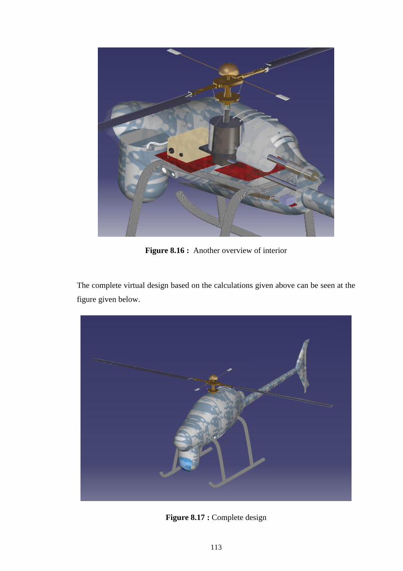
113
Figure 8.16 : Another overview of interior
The complete virtual design based on the calculations given above can be seen at the
figure given below.
Figure 8.17 : Complete design

114
Figure 8.18 : Drafting of design

115
9. CONCLUSION
Preliminary design just gives an overview to the designer at the first steps of detailed
design. The data obtained from here are all approximated values and lots of
assumptions such as constant drag coefficients can not be made during the detailed
design process. But these assumptions can be accepted as valid for preliminary
calculations.
At this work, the systems which will be used in the design was selected by trade-off
studies and a rough value of gross weight is approximated at Chapter 2. By the
selections have been done here, main rotor and tail rotors are designed with a new
gross weight iteration at Chapter 3 and Chapter 4 respectively. Then, total power
requirements were obtained and a suitable engine was selected at Chapter 5. At
Chapter 6, all rotor design process was repeated and a new concept was constructed.
All geometrical specifications of rotors were obtained at there. At Chapter 7,
helicopter’s performance analysis was made and at Chapter 8, helicopter was
drawned with the help of commercial software Catia.
Unmanned helicopters have lots of area of use. They can be used in different mission
types. At this work, the mission profile should not be considered so important
because at the payload of helicopter improved technology is used. This turret which
has seven sensors on it, is capable of doing lots of mission profiles except the
missions which needs high maneuverability. The helicopter was designed to achieve
high altitudes flights but actually the selected engine does not support above 4000
meters altitudes. At the future works, a more complicated, high performance
turboshaft engine should be selected. This gives extra weight to helicopter; but this
design is capable of flying with a turboshaft engine and its fuel required with a
reduction in mission time.

116

117
REFERENCES
[1] Bousman G.W., 2000, Aerofoil Dynamic Stall and Rotorcraft Maneuverability,
Army/Nasa Rotorcraft Division
[2] Jane’s Inc., Jane’s Unmanned Aerial Vehicles and Targets, Jane’s Information
Group, (2003).
[3] Kee S.G.,1983, Guide for conceptual helicopter design, Naval postgraduate
school.
[4] Leishman J.G., 2006, Principles of helicopter aerodynamics, Cambridge
University Press.
[5] Prouty R.W.,1985, Helicopter Aerodynamics, First edition, Potomac:Philips.
[6] Url-1 <http://www.barnardmicrosystems.com/L4E_aerial_supervisor.htm>,
accessed at 12.01.2011.
[7] Url-2 <http://www.gs.flir.com/products/airborne/cobalt190.cfm>, accessed at
04.02.2011.
[8] Url-3 < http://www.parvus.com/product/overview.aspx?prod=DuraCOR820>,
accessed at 04.02.2011.
[9] Url-4 <http://en.wikipedia.org/wiki/NOTAR>, accessed at 14.02.2011.
[10] Url-5 <http://www.engineeringtoolbox.com/dynamic-absolute-kinematic-
viscosity-d_412.html>accessed at 16.02.2011.
[11] Url-6 < http://www.ae.illinois.edu/m-selig/ads/coord_database.html#V>,
accessed at 09.04.2011.
[12] Url-7 < http://www.cfd-online.com/Wiki/NACA0012_airfoil>, accessed at
01.04.2011.
[13] Url-8 < http://www.barnardmicrosystems.com/L4E_4_stroke.htm>, accessed at
18.01.2011.
[14] Url-9 < http://www.nitto-mfg.com/nrsyokaieng.htm>, accessed at 22.01.2011.
[15] Url-10 < http://www.engineeringtoolbox.com/density-specific-weight-gravity-
d_290.html >, accessed at 24.01.2011.
[16] Url-11< http://blogs.nasa.gov/cm/blog/waynehalesblog/posts/
post_1229459081779.html >, accessed at 18.04.2011.

118

119
CURRICULUM VITAE
Candidate’s full name: Aykut Ceyhan
Place and date of birth: İstanbul / 03.09.1981
Permanent Address: Evtaş Blok. O-2 Blok. No:16 Gaziosmanpaşa/İstanbul
Universities attended: İTÜ(Astronautical Engineering)