GSM Capacity Planning-45

8/10/2019 GSM Capacity Planning-45

http://slidepdf.com/reader/full/gsm-capacity-planning-45 1/42

GSM Capacity Planning

Objective

·Learn about the basic concepts and prediction methods of capacity

planning.

·Master the network planning flow.

·Master how to increase network capacity and plan locations



Contents

1 Basic Concepts of GSM Capacity Planning...............................................................................................1

1.1 Traffic and !"#................................................................................................................................1

1.$ "all "ongestion %atio and &rlang' Table.................................................................................... .....(

2 Capacity Prediction.............................................................................................................................. ........7

$.1 Overview..............................................................................................................................................)

$.$ "apacity *rediction Method................................................................................................................)

$.$.1 +rowth Trend............................................................................................................................)

$.$.$ *opulation *enetration %ate...................................................................................................1,

$.$.( +rowth "urve.........................................................................................................................1$

$.$.- "onic.......................................................................................................................................1

$.( Traffic /istribution *rediction...........................................................................................................10

3 Capacity Planning Flow.............................................................................................................................19

(.1 "apacity *lanning deas....................................................................................................................12

(.$ *rere3uisites for "apacity *lanning.............................................................................................. ....$,

(.( "apacity *lanning "alculation Method.............................................................................................$,

(.- "hannel "apacity *lanning.......................................................................................................... .....$1

(.-.1 4/""! "apacity *lanning....................................................................................................$1

(.-.$ """! "hannel "onfiguration *rinciple................................................................................$-

(.-.( %ecommended #ssignment *rinciples for """! "hannels and T"! "hannels........... ..... .$

4 Capacity Planning pti!i"ation...............................................................................................................27

# $etwor% Capacity &!pro'e!ent...............................................................................................................29

.1 Method of mproving the 5etwork "apacity.................................................................................. ..$2

.$ #nalysis of mproving the 5etwork "apacity...................................................................................$2



.$.1 *rinciple of "ell 4plitting.......................................................................................................$2

.$.$ More #ggressive 6re3uency Multiple7ing *attern................................................................(,

.$.( #dding Microcellular &3uipment...........................................................................................(,

.$.- &7panding 6re3uency and............................................................................................... ....(1

.$. #dopting !alf %ate.................................................................................................................(1

( )ocation *rea Planning..............................................................................................................................33

0.1 /emarcating oundary of L#...........................................................................................................((

0.$ *aging "apacity of L#......................................................................................................................(-

0.$.1 #nalysis of *aging *rinciple......................................................................................... .........(-

0.$.$ *aging *olicy..........................................................................................................................(

0.$.( 4etting *aging *arameters......................................................................................................(

0.$.- "alculating L# "apacity...................................................................................................... ..(8

0.$. &ffect of 4M4 on *aging "apacity of L#..............................................................................-,



1 Basic Concepts of GSM CapacityPlanning

This document describes capacity planning of base stations on the 44 side of the

+4M network9 which serves as the basis for capacity planning of others.

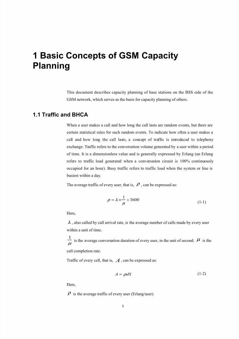
1.1 Traffic and BHCA

:hen a user makes a call and how long the call lasts are random events9 but there are

certain statistical rules for such random events. To indicate how often a user makes a

call and how long the call lasts9 a concept of traffic is introduced to telephony

e7change. Traffic refers to the conversation volume generated by a user within a period

of time. t is a dimensionless value and is generally e7pressed by &rlang ;an &rlang

refers to traffic load generated when a conversation circuit is 1,,< continuously

occupied for an hour=. usy traffic refers to traffic load when the system or line is

busiest within a day.

The average traffic of every user9 that is9 ρ 9 can be e7pressed as>

(0,,1

÷×= µ

λ ρ

!ere9

λ 9 also called by call arrival rate9 is the average number of calls made by every user

within a unit of time.

µ 1 is the average conversation duration of every user9 in the unit of second. µ is the

call completion rate.

Traffic of every cell9 that is9 A 9 can be e7pressed as>

dS A ρ =

!ere9

ρ is the average traffic of every user ;&rlang?user=.

;1'1=

;1'$=



d is the user density ;user amount? km $=.

S is the acreage of the cell ;km

$

=.

n actual environments9 traffic varies with time. &ven though the possible traffic

changes in the long'term development process are not considered9 yet traffic still

changes periodically in the short term ;on a daily or weekly basis=.

n general9 one hour when traffic is heaviest is called busy hour. #ccordingly9 the

number of calls with the one hour is the busy hour call amount or busy hour call

attempt9 that is9 !"# for short. usy traffic ;that is9 traffic within the busy hour= can

be e7pressed as>

(0,,1

÷×=

µ ρ BHCA BH

n network planning9 busy traffic is generally a design inde7 and it is believed that a

+4M network9 if supporting busy traffic9 is certainly able to deal with common traffic.

n network planning and design9 busy traffic of every user is generally used as an

inde7. usy traffic of every user can be e7pressed as>

(0,,1, ÷××= µ

β α ρ

!ere9

, ρ is busy traffic of every user.

α is the number of calls made by every user within a day.

β is the busy hour factor ;ratio of busy traffic to total traffic within a day=.

usy traffic of the system can also be e7pressed as>

N BH ×= , ρ ρ

N is the total number of users in the system.

N BH ×= , ρ ρ is a very important formula for capacity planning. t is obvious that

during system planning9 the e7pected capacity of the system must e7ceed the estimated

BH ρ .

n the current system9 the average busy traffic of every user can be obtained generally

from the statistical data of the e7isting network. t can be known from the preceding

2

;1'(=



"hapter 1 asic "oncepts of +4M "apacity *lanning

formula that the average busy traffic of every user in the current system is the total

busy traffic divided by the number of registered users on the @L% during the busy

hour. /uring network planning9 however9 some margins are generally reserved for the

average busy traffic of every user in the current system.

n "hina9 the e7perience in operating the common mobile telephone network in recent

years shows that the acceptable average busy traffic of every user is ,.,$ to ,.,(

&rl?user. This e3uals 0 calls ;including incoming and outgoing calls= made by every

user every day and $ minutes per call.

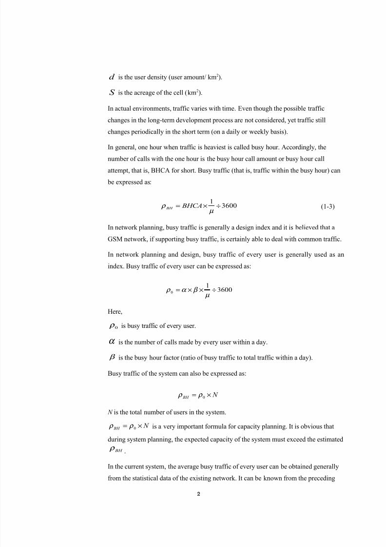
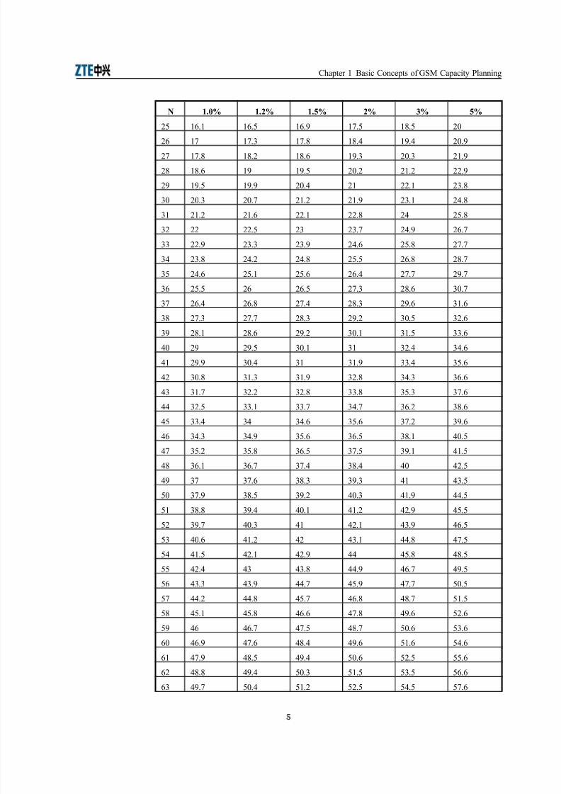
1.2 Call Congestion Ratio and Erlang-B Ta le"all loss or congestion> :hen a call is made on condition that all the channels of a

wireless communications system have already been occupied9 the call is unsuccessful

and then is lost or congested. The call congestion ratio refers to the probability that

such a call is congested.

+rade of service ;+O4= indicates the congestion level and is defined as the probability

of congestion. /uring planning of a +4M system9 +O4 of a traffic channel ;T"!= is

generally $< or <.

#s specified in the Technical Mechanism for the Common Mobile Telephone Network 9

the call congestion ratio of a wireless channel is smaller than or e3ual to <. n a high'

density traffic area9 $< is used. n general9 all common mobile telephone networks are

the call congestion systems. /uring system designs9 although a user within a cell ;or

sector= is designed to continue his or her call attempt if his or her first call cannot

occupy the idle channel9 yet the Asector sharingB or Adirected retryB function diverts the

congested call of the user to another sector for searching for an idle channel9 that is9 the

user leaves the sector that he or she originally accesses. Therefore9 for users of every

sector9 every call of users is lost if there is no idle channel9 and the result is that the

overall congestion feature is comparatively close to the &rlang' call rules.

#ccording to the &rlang call congestion formula and the call congestion calculation

table9 a call must have the following characteristics>

· &very call is random9 which is independent of or irrelevant to other calls.

· &very call has the same probability in terms of time.

· :hen a call cannot occupy the idle channel9 the call is lost9 instead of waiting a

period of time for the channel to become idle.

3



+4M "apacity *lanning

The &rlang' formula is>

This formula provides the relationship between the call congestion ratio 9 traffic #9

and channel amount n. #ccording to this formula9 you can calculate traffic at different

call congestion ratios and on different channels. The calculated traffic values form an

&rlang' table. f knowing any two of the preceding 9 #9 and n9 you can calculate the

value of the third one.

The following table is an &rlang' table formed according to calculation via the &rlang

formula and is used for convenient 3uery.

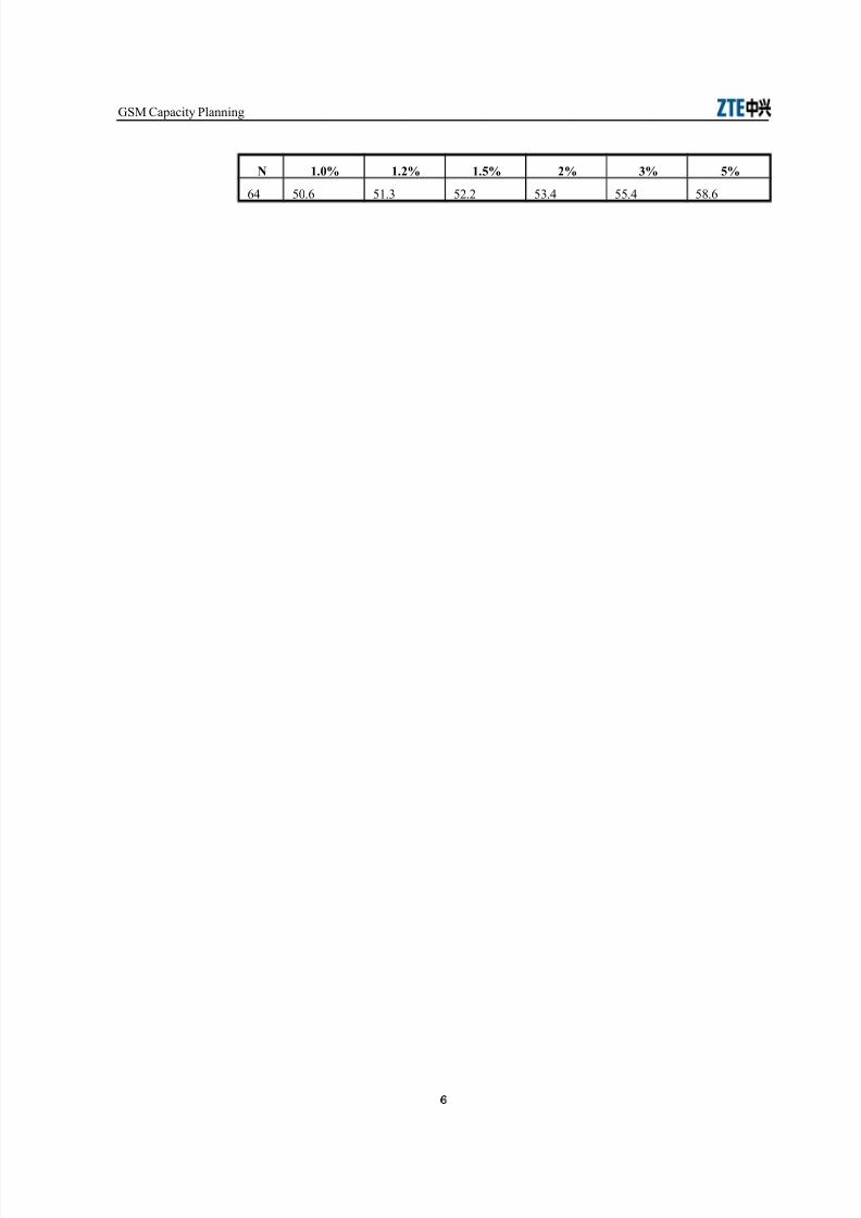
$ 1.+, 1.2, 1.#, 2, 3, #,

1 ,.,1,1 ,.,1$1 ,.,1 $ ,.,$,- ,.,(,2 ,., $0

$ ,.1 ( ,.108 ,.12 ,.$$( ,.$8$ ,.(81

( ,.- ,.-82 ,. ( ,.0,$ ,.)1 ,.822

- ,.802 ,.2$$ ,.22$ 1.,2 1.$0 1. $

1.(0 1.-( 1. $ 1.00 1.88 $.$$0 1.21 $ $.11 $.$8 $. - $.20

) $. $.0 $.)- $.2- (.$ (.)-

8 (.1( (.$ (.- (.0( (.22 -. -

2 (.)8 (.2$ -.,2 -.(- -.) .()

1, -.-0 -.01 -.81 .,8 . ( 0.$$

11 .10 .($ . - .8- 0.(( ).,8

1$ .88 0., 0.$2 0.01 ).1- ).2

1( 0.01 0.8 )., ).- ).2) 8.8(

1- ).( ). 0 ).8$ 8.$ 8.8 2.)(

1 8.11 8.(( 8.01 2.,1 2.0 1,.0

10 8.88 2.11 2.-1 2.8( 1,. 11.

1) 2.0 2.82 1,.$ 1,.) 11.- 1$.

18 1,.- 1,.) 11 11. 1$.$ 1(.-

12 11.$ 11. 11.8 1$.( 1(.1 1-.(

$, 1$ 1$.( 1$.) 1(.$ 1- 1 .$

$1 1$.8 1(.1 1(. 1- 1-.2 10.$

$$ 1(.) 1- 1-.( 1-.2 1 .8 1).1

$( 1-. 1-.8 1 .$ 1 .8 10.) 18.1

$- 1 .( 1 .0 10 10.0 1).0 12

4




$ 1.+, 1.2, 1.#, 2, 3, #,

$ 10.1 10. 10.2 1). 18. $,

$0 1) 1).( 1).8 18.- 12.- $,.2

$) 1).8 18.$ 18.0 12.( $,.( $1.2

$8 18.0 12 12. $,.$ $1.$ $$.2

$2 12. 12.2 $,.- $1 $$.1 $(.8

(, $,.( $,.) $1.$ $1.2 $(.1 $-.8

(1 $1.$ $1.0 $$.1 $$.8 $- $ .8

($ $$ $$. $( $(.) $-.2 $0.)

(( $$.2 $(.( $(.2 $-.0 $ .8 $).)

(- $(.8 $-.$ $-.8 $ . $0.8 $8.)

( $-.0 $ .1 $ .0 $0.- $).) $2.)(0 $ . $0 $0. $).( $8.0 (,.)

() $0.- $0.8 $).- $8.( $2.0 (1.0

(8 $).( $).) $8.( $2.$ (,. ($.0

(2 $8.1 $8.0 $2.$ (,.1 (1. ((.0

-, $2 $2. (,.1 (1 ($.- (-.0

-1 $2.2 (,.- (1 (1.2 ((.- ( .0

-$ (,.8 (1.( (1.2 ($.8 (-.( (0.0

-( (1.) ($.$ ($.8 ((.8 ( .( ().0

-- ($. ((.1 ((.) (-.) (0.$ (8.0

- ((.- (- (-.0 ( .0 ().$ (2.0

-0 (-.( (-.2 ( .0 (0. (8.1 -,.

-) ( .$ ( .8 (0. (). (2.1 -1.

-8 (0.1 (0.) ().- (8.- -, -$.

-2 () ().0 (8.( (2.( -1 -(.

, ().2 (8. (2.$ -,.( -1.2 --.

1 (8.8 (2.- -,.1 -1.$ -$.2 - .

$ (2.) -,.( -1 -$.1 -(.2 -0.

( -,.0 -1.$ -$ -(.1 --.8 -).

- -1. -$.1 -$.2 -- - .8 -8.-$.- -( -(.8 --.2 -0.) -2.

0 -(.( -(.2 --.) - .2 -).) ,.

) --.$ --.8 - .) -0.8 -8.) 1.

8 - .1 - .8 -0.0 -).8 -2.0 $.0

2 -0 -0.) -). -8.) ,.0 (.0

0, -0.2 -).0 -8.- -2.0 1.0 -.0

01 -).2 -8. -2.- ,.0 $. .0

0$ -8.8 -2.- ,.( 1. (. 0.0

0( -2.) ,.- 1.$ $. -. ).0

5




$ 1.+, 1.2, 1.#, 2, 3, #,

0- ,.0 1.( $.$ (.- .- 8.0

6



2 Capacity Prediction

2.1 !"er"ie#

n terms of cellular network planning9 the system capacity re3uirements must be

determined first9 that is9 how many users will be in the system and how much traffic the

users will generate. This serves as the basis of designs on the whole cellular network.

The prediction analysis of system capacity aims to reflect the actual and future capacity

re3uirements in the system so as to estimate the number of channels re3uired in the

system. 5etwork planning is implemented based on the distribution of initial and future

traffic re3uirements obtained through various statistics and calculations.

"apacity prediction needs to take into consideration the following factors>

1. ncoming status

$. /istribution of population at different age groups and incoming groups

(. #s'is economic status of the region

-. ntroduction of service competition

. %educed or preferential mobile service e7panses

0. *ublicity and development goals of mobile operators

2.2 Capacity Prediction Met$od

1. 4hort'term prediction ;1 to $ years= or long'term prediction ;( to years=

$. *opulation penetration rate

(. +rowth trend

-. +rowth curve

. "onic

2.2.1 Gro#t$ Trend

1= #s'is mobile communications outside of "hina

n Cune $,,(9 the number of mobile users worldwide has hit 1.( billion9 with a

7



penetration rate of over 18<. A%eplacement of fi7ed with mobileB has become

an increasingly obvious trend. "urrently9 over 1,, countries worldwide have

seen more mobile users than fi7ed'line users.

n &urope9 the average penetration rate of mobile phones is about ) < and the

market penetration rate is almost saturated. &uropean operators are raising

service #%*D to compensate for loss incurred by slow growth of the user base.

:hat is delightful is that the data services are on the continuous increase. n

$,,$9 revenues from the data services accounted for 1(.0< of the total revenues

in &urope9 of which the short message service took up the major part and such

services as +*%4 and :#* held less than <.

*rior to Culy $,,19 #merica was the worldEs largest mobile communications

market and its penetration rate of mobile phones was about ,<. !owever9 due

to fierce market competition9 revenues from mobile services are constrained and

the overall growth of the mobile user base is not promising. #t the same time9

along with the slowdown of #merican economy9 operators in #merica were

confronted with many difficulties. Dnder such circumstances9 it was a possible

way out of the economy shadow for the mobile communications industry to seek

out cooperation and collaboration and develop new service models.

Dnlike &urope and #merica9 Capan and 4outh Forea witnessed good results.

#lthough the proportion of mobile uses in Capan and 4outh Forea had already

e7ceeded 0,< early9 the enriched data services9 however9 brought in continuous

service revenues. *articularly9 in Capan9 the mobile data users accounted for ),<

to 8,< of the total mobile users and the proportion of revenues from the data

services e7ceeded $,<9 with the short message service taking up only (<.

n the developing countries and certain under'developing countries9 the mobile

communications services are still growing astonishingly. 4pecifically9 in over half of #frican countries9 the number of mobile users has e7ceeded that of fi7ed'

line users. n addition9 8 < of the total mobile users are prepaid users. n $,,$9

the average proportion of prepaid users was about ,< worldwide and this

figure is still on the increase.

$= #s'is mobile communications in "hina

n "hina9 the mobile communications services have been maintaining a

momentum of rapid growth. y Culy $,,19 the number of mobile users in "hina

8




surpassed that in #merica and "hina became the worldEs largest mobile

communications market. Two years later9 "hinaEs mobile user base has e7ceeded

$ ) million by October $,,( and this was the first time that the mobile user base

e7ceeded the fi7ed line user base ;$ million=. "urrently9 the penetration rate of

mobile communications in "hina is about $,<. n the ne7t five years9 this figure

will be increased greatly. "hina still lags far behind her &uropean and #merican

counterparts in terms of the overall country power and especially9 the

development in "hina is imbalanced. #ll these trigger the shift of mobile

communications from high'end users to common users. The short message

service is widely accepted and is e7plosively growing. n $,,(9 the total number

of short messages hit 18, billion. n addition9 the multimedia message service

;MM4= is gradually burgeoning. t is believed in the telecommunications

industry that the MM4 service is a rising star and also a runner for fostering the

(+ service markets.

(= Overall development trend of mobile communications

:ithin a period of time in the future9 the mobile user base continues to be

e7panded and its dominance role will be future fortified. !owever9 the

continuous efforts are still re3uired for the compliance of mobile services with

application standards. The #%*D will continue to fall until the data services are

widely accepted and booming. The voice and its value'added services will also

continue to grow and in addition9 the data services will develop continuously.

#ll these re3uire a cost'effective (+ network. The (+ network9 however9 will

grow in a step'by'step manner because considerable $+ networks e7ist and the

data services do not growth astonishingly. 6or a long period of time9 $+?$. +

and (+ technologies will coe7ist.

The following describes an e7ample of the growth trend prediction method>

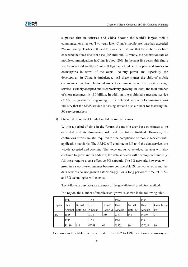
n a region9 the number of mobile users grows as shown in the following table.

%egion

122$ 122( 122- 122

Dser

#mount

+rowth

%ate ;<=

Dser

#mount

+rowth

%ate ;<=

Dser

#mount

+rowth

%ate ;<=

Dser

#mount

+rowth %ate

;<=

!G 1,8 (,(( 18, )(0) 1-( 1- (2 2)

1220 122) 1228 1222

(118, 11- -2)01 0, 2(2$$ 82 1))0 2 82

#s shown in this table9 the growth rate from 122$ to 1222 is not on a year'on'year

9




decrease. nstead9 the growth rate fluctuates irregularly. Therefore9 in $,,,9 the average

growth rate from 122$ to 12229 that is9 ),<9 is used as the growth rate. n $,,19 the

growth rate uses -,<9 slightly higher the average national level (8.8 <. This also

complies with the actual conditions of the region ;the region is a medium'siHed city=. n

$,,$9 the growth rate uses (,<.

ased on the growth trend prediction method9 the prediction of mobile users in this

region from $,,, to $,,$ is shown in the following table.

%egion

$,,, $,,1 $,,$

Dser

#mount

+rowth %ate

;<=Dser #mount

+rowth %ate

;<=Dser #mount +rowth %ate ;<=

!G (,$,$1 ), -$$8$2 -, -20)8 (,

2.2.2 Pop%lation Penetration Rate

:hen determining the penetration rate9 take into consideration the following factors>

1. *enetration rate of mobile phones in moderately developed countries in the

world

$. &7pected attainable inde7 in the ne7t several years across the country

(. Market penetration rates of operators in the current region

-. &conomic development status in the current region

The following table lists national penetration rate of mobile phones from 122 to $,,$.

Iear 122 1220 122) 1228 1222 $,,, $,,1 $,,$

Dser amount

;1,9 ,,,=(0$.2 08-.8 1(0- $-20 (-($ , ( ),10 2$12

*enetration

rate ;<=,.(,$ ,. ) 1.1- $.,8 $.0- (.82 .-, ).02

#s estimated by relevant e7perts9 in the ne7t $ to ( years9 the penetration rate of mobile

phones will hit 1,<. 6or e7ample9 in LanHhou9 an important city in 5orthwest "hina

and also a moderately developed city across the country in terms of economic

development status9 the penetration rate has reached 0<. t is e7pected that the 1,<

goal will come $ to ( years in advance9 that is9 in $,,,9 LanHhou will see the

penetration rate 1,<. The following tables show the penetration rates in LanHhou and

across the country in recent several years.

The following table shows the as'is penetration rate of mobile phones in a certain

0




region.

45 %egion

1220 122) 1228 1222

Dser

#mount ;1,9

,,,=

*enetration

%ate ;<=

Dser

#mount ;1,9

,,,=

*enetration

%ate ;<=

Dser

#mount

;1,9 ,,,=

*enetration

%ate ;<=

Dser

#mount

;1,9 ,,,=

*enetration

%ate ;<=

1 +L (118, 1.1( -2)01 1.)) 2(2$$ (.$ 1))0 2 0.1$

#s shown in the table above9 in 12289 the penetration rate in this region is already

higher than the national average. This also reflects the regionEs role as a provincial

capital city. n 12229 the penetration rate is three'fold higher than the national average.

ased on such a proportion9 from $,,, to $,,$9 the penetration rate in this region will

be about 1,<9 1 <9 and $,< respectively.

n 4hanghai and eijing9 the penetration rate of mobile users has e7ceeded 1 <. This

region is a moderately developed city and it is possible that its penetration rate is two

years behind ejing9 that is9 1 < in $,,1. Therefore9 it is acceptable that this regionEs

penetration rate in the ne7t three years is 1,<9 1 <9 and $,< respectively.

"urrently9 "hina Dnicom holds a market share of 1,< throughout the country and its

goal is to hit $,< to (,< market share. #fter the restructuring of "hina Telecom9

"hina Mobile will turn out a new picture to compete with "hina Dnicom. #nd it is

estimated that "hina DnicomEs growth of market share will slow down. ased on such

an analysis9 the market share of "hina Dnicom in this region in the ne7t three years is

estimated to be 1,<9 1 <9 and $,< respectively. #long with market development9 the

supportive measures taken by the nation for "hina Dnicom will be phased out and the

market goes in a more standardiHed manner. #s a result9 in the future9 what is more

appealing to users is service 3uality and new service offerings.

The following table shows the estimated population of this region from $,,, to $,,$.

45 %egion

1220 122) 1228 $,,, $,,1 $,,$

*opulation

;1,9,,,=

*opulation

;1,9,,,=

*opulation

;1,9,,,=

5atural

+rowth

%ate ;J=

*opulation

;1,9,,,=

*opulation

;1,9,,,=

*opulation

;1,9,,,=

1 LanHhou$)0.,2 $8,.-0 $88. 0 .2, $21.28 $2(.), $2 .-(

#ccording to the estimated population and "hina MobileEs estimated market share in

the ne7t several years9 the estimated user base of "hina Mobile in three city of this




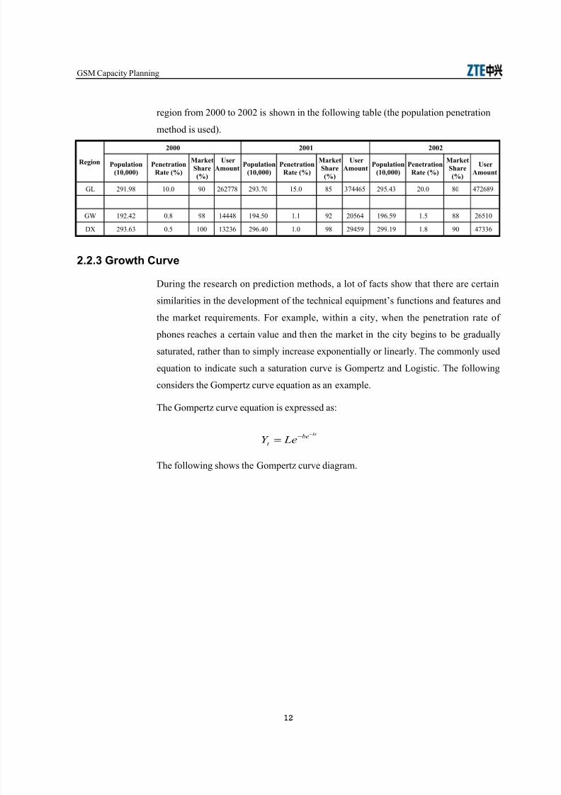
region from $,,, to $,,$ is shown in the following table ;the population penetration

method is used=.

-egion

2+++ 2++1 2++2

Pop lation/1+0+++

Penetration-ate /,

Mar%etS are/,

ser*!o nt Pop lation

/1+0+++Penetration

-ate /,

Mar%etS are/,

ser*!o nt Pop lation

/1+0+++Penetration

-ate /,

Mar%etS are/,

ser*!o nt

+L $21.28 1,., 2, $0$))8 $2(.), 1 ., 8 ()--0 $2 .-( $,., 8, -)$082

+: 12$.-$ ,.8 28 1---8 12-. , 1.1 2$ $, 0- 120. 2 1. 88 $0 1,

/G $2(.0( ,. 1,, 1($(0 $20.-, 1., 28 $2- 2 $22.12 1.8 2, -)((0

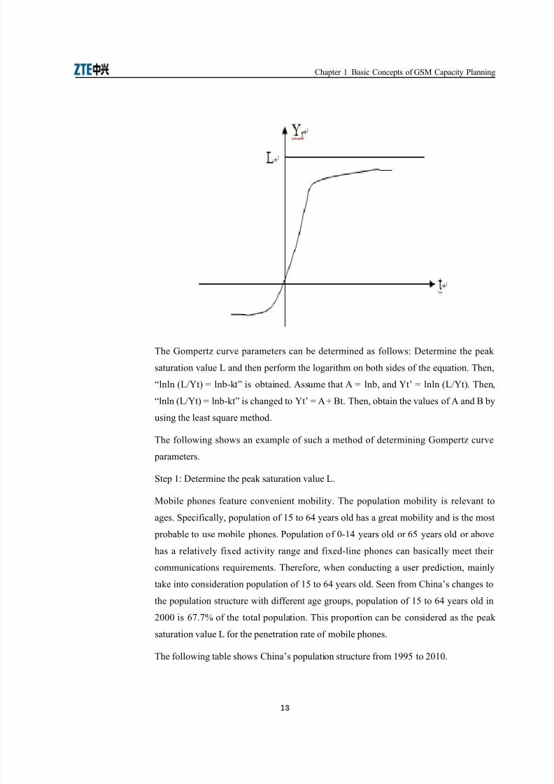
2.2.& Gro#t$ C%r"e

/uring the research on prediction methods9 a lot of facts show that there are certain

similarities in the development of the technical e3uipmentEs functions and features and

the market re3uirements. 6or e7ample9 within a city9 when the penetration rate of

phones reaches a certain value and then the market in the city begins to be gradually

saturated9 rather than to simply increase e7ponentially or linearly. The commonly used

e3uation to indicate such a saturation curve is +ompertH and Logistic. The following

considers the +ompertH curve e3uation as an e7ample.

The +ompertH curve e3uation is e7pressed as>

kt bet LeY

−−

=

The following shows the +ompertH curve diagram.

2




The +ompertH curve parameters can be determined as follows> /etermine the peak

saturation value L and then perform the logarithm on both sides of the e3uation. Then9

Alnln ;L?It= K lnb'ktB is obtained. #ssume that # K lnb9 and ItE K lnln ;L?It=. Then9

Alnln ;L?It= K lnb'ktB is changed to ItE K # t. Then9 obtain the values of # and by

using the least s3uare method.

The following shows an e7ample of such a method of determining +ompertH curve

parameters.

4tep 1> /etermine the peak saturation value L.

Mobile phones feature convenient mobility. The population mobility is relevant to

ages. 4pecifically9 population of 1 to 0- years old has a great mobility and is the most

probable to use mobile phones. *opulation of ,'1- years old or 0 years old or above

has a relatively fi7ed activity range and fi7ed'line phones can basically meet their communications re3uirements. Therefore9 when conducting a user prediction9 mainly

take into consideration population of 1 to 0- years old. 4een from "hinaEs changes to

the population structure with different age groups9 population of 1 to 0- years old in

$,,, is 0).)< of the total population. This proportion can be considered as the peak

saturation value L for the penetration rate of mobile phones.

The following table shows "hinaEs population structure from 122 to $,1,.

3




ear

5otal Pop lation +614 ears ld 1#6(4 ears ld (# ears ld or * o'e

Pop lationProportion

Pop lation*!o nt /1+0

+++


Pop lation*!o nt/1+0 +++


Pop lation*!o nt /1+0

+++


Pop lation*!o nt/1+0 +++

122 1,, 1$11$1 $0.) ($(,( 00.0 8,)$) 0.) 8,21

1220 1,, 1$$$-8 $0.- ($$)( 00.8 8100$ 0.8 8(1(

122) 1,, 1$((8 $0.1 ($$,( 0) 8$008 0.2 8 1-

1228 1,, 1$- ($ $ .8 ($1$2 0).$ 8(080 ) 8)1)

$,,, 1,, 1$08 2 $ .( ($1, 0).) 8 8-1 ) 821(

$,, 1,, 1(1-(8 $$.2 (,,22 02. 21( , ).0 2282

$,1, 1,, 1(018( $,.) $8$-8 )1.1 20)22 8.$ 111(0

4tep $> "alculate the values of # and . The following table considers a city +L as an

e7ample.

ear S$ /t ser *!o nt / t t8 lnln/): t tt8 t; t8 t2

1220 1 (118, 1.-$$200 1.-$$200,-$ 1

122) $ -2)01 1.(,(--- $.0,088)0- -

1228 ( 2(2$$ 1.11-,00 (.(-$128 $( 2

1222 - 1))0 2 ,.8)2(-- (. 1)()),1- 10

4um 1, ( $ $$ -.)128$, 1,.882-$2$$ (,

Obtain the values of # and by using the least s3uare method and set up a mathematic

model as shown below>

.$-

1,9- === t n

4




t et e y

18$,$-.,1$2 -,.12)0),−

−=

1$2 -.918$,$-., ===−= Aeb B K

0( ,$.1NO =−= t B y A t

18$,$-.,N

NNN$$

OO

−=−

−=

∑∑

t nt

yt n yt B t t

-

)128$.-O =t y

*redict the user amount of the city +L in $,,, and apply tK to the preceding formula.

Then9 obtain y$,,,K$ ,8,-. Likewise9 apply tK0 and tK)9 then obtain y$,,1K( (0$2

and y$,,$K-),822 respectively.

The following table shows the predicted mobile user amount of the city +L from $,,,

to $,,$ by using the growth curve method.

S$ -egionser *!o nt

2+++ 2++1 2++2

1 +L $ ,8,- ( (0$2 -),822

#ny type of telecommunications service needs to go through four phases9 debut9

growth9 saturation9 and degradation. 6or any service having such four phases9 you can

use the growth curve method to perform prediction and this method is very suitable to

medium'term prediction.

2.2.' Conic

6or many engineering problems9 it is a common practice to search out an appro7imatee7pression for the function relationship of two variables according to several groups of

lab data for these two variables. The appro7imate e7pression is generally called

empirical formula. #fter an empirical formula is set up9 certain e7perience accumulated

during production and e7periments can be raised to the theory for analysis. /uring a

mobile user prediction9 an empirical formula can be set up based on the user

development over the last several years and through the empirical formula9 the ne7t

several yearsE user development can be predicted.

n a city9 the growth of mobile users can be e7pressed by the following empirical

5




formula>

cba y ++= $

!ere9 7 represents the year and y the amount of mobile users.

#pply the user amount of the last several years and select constants a9 b9 and c by using

the least s3uare method.

σ $ $ $

1

= − + +=

∑P ; =Q y a b ci

N

The values of a9 b9 and c are calculated as follows>

,=Q;P

,=Q;P

,=Q;P

1

$$

1

$$

1

$$$

∑

∑

∑

=

=

=

=++−=

=++−=

=++−=

N

iiii

N

iiiii

N

iiiii

cba yc

cba yb

cba ya

∂ ∂σ

∂ ∂σ

∂ ∂σ

#pply the mobile user data of the city +L from 1220 to 1222 and then calculate thevalues of a9 b9 and c. Then9 based on the values9 you can predict the mobile user

amount of the city +L in the ne7t three years.

The following table shows the predicated mobile user amount of the city +L from $,,,

to $,,$ by using the conic method.

S$ -egionser *!o nt

2+++ 2++1 2++2

1 +L $8)()1 -(,)2, 0,018-

2.& Traffic (istri %tion Prediction

Traffic is mainly centraliHed in medium and large'siHed cities. &specially9 in the center

of an urban area9 there is a comparatively high'density traffic region. :ithin the region9

an area with e7tremely heavy traffic generally e7ists. n the suburban areas9 traffic is

low. :hen constructing a network9 take into consideration all the preceding factors and

deploy nodes properlyR otherwise9 the e3uipment resources for the low traffic areas will

be wasted and the capacity in the heavy traffic areas will be insufficient9 thus adversely

affecting the return on investments ;%O = and service 3uality of the network. To avoid

6




the preceding adverse impact9 conduct a prediction and survey of traffic distribution

beforehand and then based on the prediction and survey result9 deploy base stations and

determine the fre3uency multiple7ing mode.

#t early stages9 you can use such statistical data as population distribution9 incoming

status9 vehicle use distribution9 and phone use to predict the geographic distribution of

traffic re3uirements. #fter a network is built out and runs in the normal state9 you can

use the traffic statistical report of OM" to obtain a comparatively comprehensive

traffic distribution of the mobile service area for future optimiHation and capacity

e7pansion.

Three methods are currently available to the traffic density prediction> percentage' based method9 linear prediction method9 and linear prediction manual adjustment.

*ercentage'based method> The service area is divided into several sub'areas9 such as9

high'density user sub'area9 medium'density user sub'area9 and low'density user area

;for e7ample9 densely populated urban area9 common urban area9 and suburban area=

and then different percentages are allocated to these areas during the mobile user

prediction. Then9 multiply the predicated user amount by the percentage of an area to

obtain the total user amount of the area9 and then divide this total user amount by the

acreage of the area to obtain the user density of the region.

Linear prediction method> ased on the cell planning software and the digital map9

allocate the actual statistical busy traffic of the e7isting base stations to every cell9 and

then import the total traffic in the target year to the *". Then9 the cell planning

software can generate the traffic distribution diagram in the target year according to the

e7isting traffic distribution.

7



& Capacity Planning )lo#

ased on the preceding traffic prediction and traffic distribution prediction9 you can

obtain the total traffic re3uirements within the service area and the traffic distribution

and acreage within every specific area.

#fter a correct predication of user development within the planned area9 select a proper

fre3uency multiple7ing mode according to the available fre3uency band resources. n

addition9 after considering the configured capabilities of wireless system products as

well as the wireless environment?user distribution characteristics within the planned

area9 determine site'type configuration for different types of area and ultimately obtain

the site 3uantity that meets capacity re3uirements. "apacity planning needs to yield the

following results>

· 5umber of base stations that meet traffic re3uirements within the planned area

· 4ite'type configuration of every base station

· 5umber of traffic channels and users and traffic provided by every sector

· 5umber of traffic channels and users and traffic provided by every base station

· 5umber of traffic channels and users and traffic provided by the whole network

The preceding planning is an initial planning. That is9 after wireless coverage planning

and analysis9 certain base stations may be added or deleted. Then9 the number of base

stations and their locations are finally determined after repeated planning and analysis.

&.1 Capacity Planning *deas# common capacity planning flow is> conducting capacity prediction 'S analyHing

traffic distribution 'S determining site'type configuration 'S determining the number of

base stations 'S determining the layout of base stations.

#t different stages of network planning9 the work focuses are also different>

· #t the ele!entary stage of network development9 t ere are a few capacity

re< ire!ents 9 the site is generally small9 and the network is relatively simple.

n this case9 mainly consider the basic coverage.

9



#t the inter!ediate stage of network development9 t ere are a large n ! er

of capacity re< ire!ents 9 the coverage re3uirements are high9 and the network

is relatively comple7. n this case9 take such measures as capacity e7pansion of

base stations and cell splitting.

#t the ad'anced stage of network development9 t ere are enor!o s capacity

re< ire!ents 9 the hole'free coverage is re3uired9 and the network is comple7.

n this case9 take such measures as adding micro cells and setting up dual'

fre3uency networks.

&.2 Prere+%isites for Capacity Planningefore a prediction of total traffic and traffic distribution9 the following prere3uisites

are met>

· +O4 provided by the system ;call congestion ratio=

· #vailable fre3uency band resources and fre3uency multiple7ing mode

&.& Capacity Planning Calc%lation Met$od

&stimate the number of base stations and their types and capacity in thecapacity'constrained area.

&stimate the ma7imum site type for different types of area according to the

available fre3uency band resources and fre3uency multiple7ing mode.

Obtain the capacity of every base station according to the traffic model and

&rlang' table.

Obtain the number of re3uired base stations by dividing the total traffic by the

ma7imum capacity ;sum of capacity of all cells= of a base station.

&stimate the number of base stations and their types and capacity in the

coverage'constrained area.

Obtain the total number of base stations re3uired by a type of area by dividing

the area acreage by the coverage acreage ;estimated= of every base station.

Obtain the re3uired traffic within a cell by multiplying the coverage acreage

;estimated= of the cell by the corresponding traffic density.

&stimate the number of re3uired voice channels and control channels according

20




to the &rlang' table.

Obtain the number of re3uired carrier fre3uencies of a cell by dividing the sumof the voice channels and control channels by 8.

The output results are total number of base stations and their types.

The following is an e7ample of calculating capacity of a base station.

n an 4-?-?- base station9 every cell has ($ channels9 of which $2 are traffic channels.

#ssume that the call congestion ratio is $<. #ccording to the &rlang' table9 it is

found that traffic carried in this base station is $1.,( &rl. #ssume that the average busy

traffic of every user is ,.,$ &rl9 then9 it is calculated that 8-1 users can be

accommodated. Then9 the whole base station can accommodate $ $( users ;8-1 7 ( K

$ $(=.

&.' C$annel Capacity Planning

&.'.1 S(CCH Capacity Planning

1. S=CC> c annel str ct re and ser'ice type

#n 4/""! channel has two types of structure> 4/""!?- and 4/""!?8. These twotypes of structure are applied to the hybrid control channel and independent control

channel respectively. n a +4M system9 the cell broadcast service can be provisioned.

That is9 within an area9 the short messages of the short message service center are

broadcast to all registered users within the area. :hen the cell broadcast service is

provisioned9 the broadcast traffic channel " "! of every cell must occupy an 4/""!

channel.

"ombined channel>

""! """! 4/""!?- ;T4,=

5on'combined ;independent= channel>

""! """! ;T4,= G 7 4/""!?8 ;timeslots for ""! carriers fre3uencies 1') or

any timeslot for other carrier fre3uencies=

/uring network designs9 G can be configured according to the number of carrier

fre3uencies ;that is9 number of T"! channels= and the proportion of T"! traffic to

4/""! traffic.

2




#n 4/""! channel mainly carries the following types of services>

· Location update or periodic location update

· M4 attachment?separation

· "all set'up

· 4hort message

· 6a7 and supplementary services

6or networks with different structures and user habits and for different traffic models9

time when the preceding various events are occupying the 4/""! channel is also

different.

2. S=CC> G S and S=CC>:5C> capacity proportion

:hen the number of 4/""! channels is defined9 the call congestion ratios of 4/""!

channels and T"! channels must be comprehensively considered. This is because in a

conversation9 4/""! channels are used to transmit the call connection signaling and

T"! channels are used to transmit voice or data information. 4/""! channels and

T"! channels are e3ually important for set'up of a conversation. 4/""!9 however9

can utiliHe the physical channels of carrier fre3uencies in a more effective manner.

Therefore9 the call congestion ratio of 4/""! channels must be lower than that of

T"! channels.

The basic principles for determining the call congestion ratio of 4/""! channels are

as follows> The call congestion ratio of 4/""! channels must be $ < of that of T"!

channels. f the call congestion ratio of 4/""! channels is higher than $ < of that of

T"! channels9 more 4/""! channels must be defined. 6or the 4/""!?- structure9

the call congestion ratio of 4/""! channels must be ,< of that of T"! channels.

n general9 the +O4 of the 4/""!?8 structure is calculated as 1?- of the +O4 of T"!.The +O4 of the 4/""!?- structure is calculated as 1?$ of the +O4 of T"!.

6or e7ample9 when the +O4 of T"! is $<>

· 4/""!?- +O4 K 1<

· 4/""!?8 +O4 K ,. <

ased on the channel assignment algorithm of 4"9 signaling can be transmitted on

the T"! channels. 5o matter which channel assignment method ;pre'assignment or

dynamic assignment= is used9 signaling both can be transmitted on the T"! channels.

22




/uring set'up of a call9 T"! channels are immediately assigned for transmitting call

connecting signaling. This can reduce call congestion ratio and improve +O4.

3. S=CC> Capacity Prediction

4/""! traffic prediction is calculated according to common service models. /ifferent

networks and traffic models have different 4/""! traffic models. /uring actual

4/""! planning9 make calculations according to the service models provided by

operators.

f the service models have already been provided9 you can calculate per'user traffic of

every type of phone action.

The corresponding calculation formula is as follows>

The following shows the calculation process ;only considering location update9 short

message9 and call set'up=>

"onventions>

· Location update factor> L

· *roportion of short message amount to call amount> 4

· #verage call duration> T

· "ell traffic> #cell

· Location update duration> TLD· "all set'up duration> T"

· 4hort message duration> T4M4

· 4/""! clear protection duration> T+

Then9

· usy call amount of a cell> U"#LL K #cell 7 (0,,?T

· usy location update amount> ULD K L 7 #cell 7 (0,,?T

23




· usy short message amount> U4M4 K 4 7 #cell 7 (0,,?T K 0#cell

Then9 traffic carried by 4/""! is>

#4/""! K PU"#LL 7 T" ULD 7 ;TLD T+= U4M4 7 ;T4M4 T+=Q?(0,,

#fter traffic is obtained9 you can obtain the number of re3uired 4/""! channels from

the &rlang' table according to the corresponding +O4.

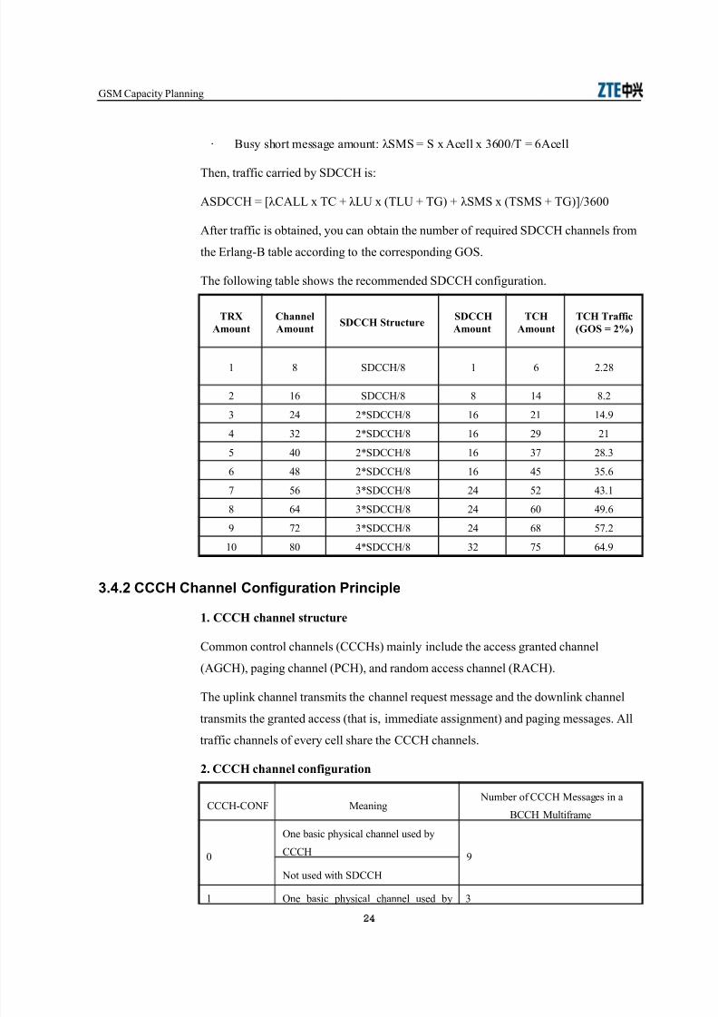
The following table shows the recommended 4/""! configuration.

5-?*!o nt

C annel*!o nt

S=CC> Str ct re S=CC>*!o nt

5C>*!o nt

5C> 5raffic/G S 2,

1 8 4/""!?8 1 0 $.$8

$ 10 4/""!?8 8 1- 8.$

( $- $N4/""!?8 10 $1 1-.2

- ($ $N4/""!?8 10 $2 $1

-, $N4/""!?8 10 () $8.(

0 -8 $N4/""!?8 10 - ( .0

) 0 (N4/""!?8 $- $ -(.1

8 0- (N4/""!?8 $- 0, -2.0

2 )$ (N4/""!?8 $- 08 ).$

1, 8, -N4/""!?8 ($ ) 0-.2

&.'.2 CCCH C$annel Config%ration Principle

1. CCC> c annel str ct re

"ommon control channels ;"""!s= mainly include the access granted channel

;#+"!=9 paging channel ;*"!=9 and random access channel ;%#"!=.

The uplink channel transmits the channel re3uest message and the downlink channel

transmits the granted access ;that is9 immediate assignment= and paging messages. #ll

traffic channels of every cell share the """! channels.

2. CCC> c annel config ration

"""!'"O56 Meaning 5umber of """! Messages in a

""! Multiframe

,

One basic physical channel used by

"""! 2

5ot used with 4/""!

1 One basic physical channel used by (

24




"""!'"O56 Meaning 5umber of """! Messages in a

""! Multiframe

"""!

Dsed with 4/""!

$

Two basic physical channels used by

"""! 18

5ot used with 4/""!

-

Three basic physical channels used by

"""! $)

5ot used with 4/""!

0

6our basic physical channels used by

"""! (0

5ot used with 4/""!

&.'.& Reco,,ended Assign,ent Principles for CCCH C$annels and TCHC$annels

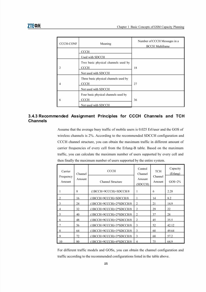
#ssume that the average busy traffic of mobile users is ,.,$ &rl?user and the +O4 of

wireless channels is $<. #ccording to the recommended 4/""! configuration and

"""! channel structure9 you can obtain the ma7imum traffic in different amount of

carrier fre3uencies of every cell from the &rlang' table. ased on the ma7imum

traffic9 you can calculate the ma7imum number of users supported by every cell and

then finally the ma7imum number of users supported by the entire system.

"arrier

6re3uency

#mount

"hannel

#mount

"""!"ontrol

"hannel

#mount

;4/""!=

T"!

"hannel

#mount

"apacity

;&rlang=

"hannel 4tructure +O4K$<

1 8 ;1 ""! 2"""!= 4/""!?8 1 0 $.$8

$ 10 ;1 ""! 2"""!= 4/""!?8 1 1- 8.$

( $- ;1 ""! 2"""!= $N4/""!?8 $ $1 1-.2- ($ ;1 ""! 2"""!= $N4/""!?8 $ $2 $$

-, ;1 ""! 2"""!= $N4/""!?8 $ () $8

0 -8 ;1 ""! 2"""!= $N4/""!?8 $ - ( .

) 0 ;1 ""! 2"""!= (N4/""!?8 ( $ -$.1$

8 0- ;1 ""! 2"""!= (N4/""!?8 ( 0, -2.0-

2 )$ ;1 ""! 2"""!= (N4/""!?8 ( 08 ).$

1, 8, ;1 ""! 2"""!= -N4/""!?8 - ) 0-.2

6or different traffic models and +O4s9 you can obtain the channel configuration and

traffic according to the recommended configurations listed in the table above.

25




26



' Capacity Planning !pti,i ation

The initial capacity planning is mainly based on various predications and assumptions.

#s network planning and network construction are implemented9 traffic models may

change and these changes to traffic models ;such as change to the siHe of a traffic

model= have a direct and important impact on capacity planning. n actual conditions9

the initial capacity planning will be adjusted and optimiHed9 thereby laying a good

foundation for future network optimiHation and reducing investments under certainconditions.

The recommended traffic model calculation method on the e7iting network is as

follows>

:hen any of the following factors occurs9 you need to consider adjusting and

optimiHing capacity planning>

"hanges to user behavior> Mainly consider the user capacity offset caused by

mobility of users in the local network. Dse behavior includes user traffic

behavior and user mobility behavior. These two types of behavior lead to user

traffic offset from the macro and micro perspectives respectively. #s for the

e7tent to which the traffic offset affects the network9 we can use the fluctuation

coefficient ;1., '1.1 in general= for measurement. The network margins caused by such offset cannot be saved during network construction.

5on'linear channel configuration> "hannel configuration is calculated according

to the number of carrier fre3uencies rather than linearly based on re3uirements.

This certainly leads to wastes. 6or e7ample9 a cell only needs 2 T"! channels9

but we need to configure $ T%Gs ;that is9 1- T"! channels=. This means that

T"! channels are wasted. #ccording to domestic network research and

e7perience and statistics of several local networks9 non'linear channel

configuration decreases network utiliHation by $,< to $ <. 6or provincial

27



capital cities9 the figure is $,< and for common cities9 the figure is $ <.

&specially9 for the backward areas9 the figure is (,< because there are many

single'carrier'fre3uency cells.

#t early stages of network construction9 if heavy traffic congestion occurs9 you

need to consider the suppressed traffic re3uirements due to traffic congestion

when performing a traffic model prediction. 4pecifically9 add the traffic re3uired

for solving traffic congestion as the actual traffic to the traffic model. Then9 the

traffic model is a true traffic model that meets actual conditions.

#t different stages of network construction9 it is proper to carry out an analysis

and prediction of traffic models periodically.

f the predicted proportion of activated mobile users is relatively proper9 take

into consideration this proportion. This can reduce the traffic model value of

every user9 and reduce costs of base stations or compensate for impact caused by

other uncontrollable factors.

Other impacts.

28



/et#or0 Capacity *,pro"e,ent

n the initial stage of a +4M network9 the number of users is limited9 and in this case9

fewer T4s with small model are suitable for the network capacity. n this situation9

the main problem is network coverage. :ith the rapid user development and new

service promotion9 cell congestion is more and more severe and the network 3uality is

attacked. Therefore9 it is urgent to improve the network capacity. The process of the

capacity design is>

T4 with small model'S T4 e7pansion and cell splitting'SMicrocellular increase in

hot stop'STwo fre3uency construction'S!alf rate provisioning

.1 Met$od of *,pro"ing t$e /et#or0 Capacity

#dopting cell splitting

#dopting the more aggressive fre3uency multiple7ing pattern

#dding microcellular e3uipment

&7panding fre3uency band

#dopting half rate

.2 Analysis of *,pro"ing t$e /et#or0 Capacity

.2.1 Principle of Cell Splitting

n the initial stage of a +4M network9 the network coverage is the main problem. This is because the antenna height is high9 distance between T4s is

large9 and the coverage radius is large.

:ith the user increment9 the original cell can be split into cells with smaller

coverage area.

4horten the distance between T4s9 lower the antenna height9 or increase the

antenna downtilt angle appropriately9 so as to narrow the coverage radius.

Through cell splitting9 increase the number of T4s in the network9 and then the

29



carrier fre3uencies and channels of the entire network increase9 accordingly9 the

traffic and users are accommodated.

Method of implementing cellular splitting

#dd a new T4 at the center point of the connection line between two e7isting

T4s.

Dse half of the radius of the e7isting cell as the radius of the split cell and the

antenna direction of sectors after splitting remains unchanged.

"ell splitting is limited and the distance of macro'cellular T4s is at least -,,m.

The antenna height of a T4 cannot be very high. That is9 in a medium siHe city9 theantenna height is about $ m.

6or a T4 with high antenna height9 lower the height in cell splitting.

.2.2 More Aggressi"e )re+%ency M%ltiple ing Pattern

f the network capacity cannot be increased through cell splitting9 the more aggressive

fre3uency multiple7ing pattern can be used. That is9 improve the fre3uency band usage

and enlarge the T4 model supported by the network9 so as to improve the network

capacity.

The common aggressive fre3uency multiple7ing patterns are>

Multiple multiple7ing pattern ;M%*=

1 7 ( ;or 1 7 1= multiple7ing

"oncentric circle

.2.& Adding Microcell%lar E+%ip,ent

Two cases for microcellular> One is to improve the coverage blind Hone and the

other is to solve the problem of traffic overflow of the hot spot with high traffic.

The macro'cellular with large coverage is in the lower layer and absorbs the

main traffic. The micro'cellular is with a higher layer and is the supplement of

the macro'cellular coverage9 which improves the indoor coverage9 absorbs the

traffic of the hot spot9 and improves the network 3uality.

.2.' E panding )re+%ency Band

Through e7panding the fre3uency band9 increase the carrier fre3uency of each30



3ocation Area Planning

Location area ;L#= is an important concept in +4M. #ccording to the +4M protocol9

the entire mobile communication network is divided into different service areas based

on location area code ;L#"=. L# is the unit for paging scope in a +4M system. That is9

the paging message pages in the unit of L#. The paging message of a mobile

subscriber is sent in all the cells of an L#. One L# may contain one or more base

station controllers ; 4"= but it belongs to only one mobile switch center ;M4"=. naddition9 one 4" or M4" may contain multiple L#s.

The siHe of an L#9 the coverage of an L#"9 is a key factor in the system. n the aspect

of decreasing the location update fre3uency and economiHing the channel resources of

a system9 the bigger the L# is the better. This is because the more the location update9

the bigger the 4/""! load9 which wastes the channel resources and increases the

M4" and !L% load. n addition9 the mobile station re3uires about 1,s to update cells.

n this period of time9 a call cannot be made. !owever9 if an L# is over siHe and is

beyond the paging capability of the system9 the paging signaling load in the system isvery high9 which leads to paging message loss and decrement of the paging success

ratio. The low paging success ratio generates the second call for a subscriber. n this

case9 the paging load in the system increases and the paging success ratio deteriorates.

Therefore9 the L# cannot be set to a large value. n network planning9 consider and

balance the L# capacity9 channel resources and paging capability in the system. n the

case that the paging load is not very high9 decrease the update fre3uency of the L# to a

minimiHed value.

.1 (e,arcating Bo%ndary of 3A

n the initial stage of a +4M network9 T4s in multiple 4"s can be divided into an

L#. :ith the increase of traffic and carrier fre3uency capacity9 the traffic carried by

each 4" increases greatly and L# demarcation approaches to 4" demarcation. That

is9 one 4" is demarcated to one L#. n a fewer cases9 one 4" can be demarcated to

multiple L#s. !owever9 problems may arise because of the very small L#. 6or

e7ample9 inter'L# update occurs more fre3uently and thus the switch load increases.

:hen location update occurs in different L#s9 a mobile phone cannot communicate33



normally. n density urban areas with high traffic9 a mobile phone is active in the

overlap areas of different L#s. n this case9 a high re3uirement for boundary setting of

two L#s or multiple L#s is re3uired. :ith the network development9 user density

increases and the effect of inter'L# update on the system load increases. Therefore9 the

boundary setting of L#s is more important. #ccording to features of the normal

location update9 boundary demarcation of the L# needs to comply with the following

principles>

Try not to set the boundary away from the areas with high traffic such as urban

areas9 instead9 set it in areas with low traffic or for low'end users such as rural

areas and factories. These areas are with low density9 location update scope of

the mobile phone narrows9 and inter'L# update has relatively lower load for the

network. :hen the L# boundary should cover the urban areas9 try to set the

boundary in the areas with low mobility such as residential areas.

4et the L# boundary and the road with an angle and try to prevent the overlap

areas of the L# from being in the areas with high mobility. This avoids a large

amount of toggle location update in inter'L#. f the setting is improper9 the

system will be severely affected.

The boundary of multiple L#s is avoided in the same small area9 and this prevents the mobile phone from fre3uently updating among location areas in the

small area.

:hen demarcating the boundary9 the traffic increase trend needs to be taken into

consideration. n addition9 in designing paging capacity and traffic capacity of

an L#9 the e7pansion margin needs to be considered9 so as to prevent the L#

from demarcating and splitting fre3uently.

.2 Paging Capacity of 3A

.2.1 Analysis of Paging Principle

:hen a mobile station of an L#" is paged9 the M4" initiates the paging re3uest for all

the cells corresponding to the L#" through 4". "urrently9 the +4M network

provides two paging modes> TM4 and M4 .

n the +4M system9 each user is allocated with a uni3ue M4 . The M4 is written in

the 4 M card of a mobile phone9 and it is with eight bytes and is used for identity

34



"hapter 0 Location #rea *lanning

identification. The TM4 is allocated temporarily by the @L% for the visited mobile

subscriber after successful authentication. The TM4 is temporarily used for the air

interface instead of the M4 only in the @L% jurisdictional areas. n addition9 TM4

corresponds to M4 and is with four bytes. n this case9 when the paging channel of

the air interface adopts M4 9 the paging re3uest contains only two M4 numbersR but

if TM4 is adopted9 four TM4 numbers are contained. Therefore9 paging load of M4

is twice more than that of TM4 .

:hen obtaining current L# of the mobile station from @L%9 M4" initiates the paging

message to all the 4"s in the L#. #fter receiving the paging message9 4"s send the

paging message to all the cells belonging to the L# of the 4"s. :hen receiving the

paging message9 T4 sends the paging re3uest to paging sub'channels where the

paging group is located. The paging re3uest carries M4 or TM4 of the paged user.

#fter receiving the paging re3uest9 the mobile station uses the random access channel

;%#"!= to allocate 4/""!. n addition9 after confirming that the T4 activates the

re3uired 4/""!9 4" assigns the 4/""! to the mobile station by assigning the

message in the access grant channel ;#+"!=. Then9 the mobile station uses the

4/""! to send the paging response to 4" and 4" forwards the paging response to

M4". n this case9 a successful radio paging is complete.

.2.2 Paging Policy

f the M4 L# is known in @L%9 the first paging message is broadcasted in the L#s that

are registered in M49 that is9 local paging. f M4 does not respond to the first paging9

M4" initiates the second paging. Dsually9 the second paging is broadcasted in the

original L#. !owever9 the second paging can be performed in all the cells in the entire

M4"9 that is9 global paging. The global paging is with a higher success ratio. n paging9

TM4 or M4 can be used to differentiate M4.

.2.& Setting Paging Para,eters

#ccording to the +M4 specifications9 """! has two configurations>

4hared """! and 4/""!9 also called combined ""!. n this configuration9

each multiframe transfers three paging groups.

Dn'shared """! and 4/""!9 also called un'combined ""!. n this

configuration9 each multiframe transfers nine paging groups.

The paging group can be used as the paging channel ;*"!= to broadcast the paging

35




re3uest9 and can be used as the #+"! to respond the access re3uest of a mobile phone.

n operation9 multiple multiframes can be combined together so as to form a paging

cycle to increase the number of paging groups in a cell. n this case9 the mobile phone

senses its belonged paging group periodically. Therefore9 when the mobile phone is

called9 it monitors the paging re3uest sent from the T4 and responds.

f there are many paging groups9 a long time will be cost before the mobile phone

monitors the correct paging group. This increases the paging time. f there are fewer

paging groups9 the paging setup time will be shortened because the mobile phone

answers the paging group fre3uently. This wastes electricity of the mobile phone. The

number of paging groups of a cell can be adjusted through the following two

parameters>

#ccess grant reserved blocks ; 4'#+' LF'%&4=

This parameter defines the number of paging groups that are configured with the

dedicated #+"! of each multiframe. 6or the cell with combined ""!9 4'#+'

LF'%&4 ranges from , to $. 6or the cell with un'combined ""!9 4'#+' LF'

%&4 ranges from , to ). f the cell broadcast channel ;" "!= is used9 4'#+' LF'

%&4 ranges from 1 to ). The value of 4'#+' LF'%&4 can be ,9 it indicates that no

dedicated #+"! is used9 and all the paging groups are shared by *"! and #+"!. f 4'#+' LF'%&4 is e3ual to or larger than 19 it indicates that a paging group is

reserved as the dedicated #+"!. This is determined by the traffic of the cell.

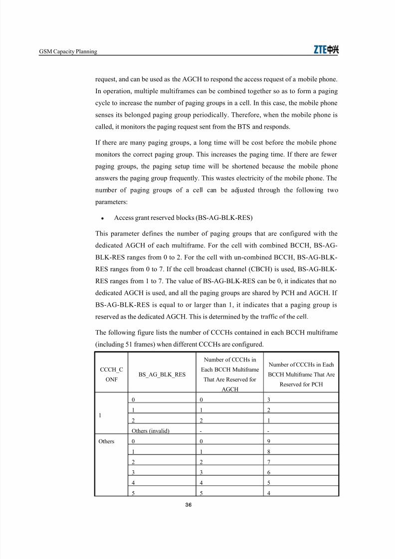
The following figure lists the number of """!s contained in each ""! multiframe

;including 1 frames= when different """!s are configured.

"""!V"

O564V#+V LFV%&4

5umber of """!s in

&ach ""! Multiframe

That #re %eserved for

#+"!

5umber of """!s in &ach

""! Multiframe That #re

%eserved for *"!

1

, , (

1 1 $

$ $ 1

Others ;invalid= ' '

Others , , 2

1 1 8

$ $ )

( ( 0

- -

-

36




"""!V"

O564V#+V LFV%&4

5umber of """!s in

&ach ""! Multiframe

That #re %eserved for #+"!

5umber of """!s in &ach

""! Multiframe That #re

%eserved for *"!

0 0 (

) ) $

*aging channel multiframes ; 4'*#'M6%#M4=

This parameter defines multiframes in 1 T/M# frames of M4 of the same paging

group that are sent by the transmission paging message. #ccording to the +4M

specifications9 each mobile subscriber ;corresponding to each M4 = belongs to a

paging group. n every cell9 each paging group corresponds to a paging sub'channel.

The mobile station calculates to which paging group it belongs based on its M4 .

Then9 it calculates the location of the paging sub'channel that belongs to the paging

group. n an actual network9 the mobile station just listens the paging sub'channel to

which it belongs but not listen the contents of other paging sub'channels. n addition9

disable the power of certain hardware components of the mobile station to save the

power cost ;source of /%G=. s*aMframes refers to a cycle with how many

multiframes that are used as the paging sub'channels. #ctually9 this parameter

determines the number of paging sub'channels of the paging channels in a cell."alculation of this parameter is mainly used to calculate the paging group of M49 so as

to sense the corresponding paging sub'channels.

The following tables lists the relation between #+"! and M6%M49 and number of

paging group and paging group interval.

4V*#V

M6%#M

4

*aging +roup

nterval ;s=

5umber of *aging +roups in

"ombined ""!

5umber of *aging +roups in Dn'

combined ""!

#+"!K, #+"!K1 #+"!K, #+"!K1

$ ,.-) 0 - 18 10( ,.)1 2 0 $) $-

- ,.2- 1$ 8 (0 ($

1.18 1 1, - -,

0 1.-1 18 1$ - -8

) 1.0 $1 1- 0( 0

8 1.82 $- 10 )$ 0-

2 $.1$ $) 18 81 )$

37




.2.' Calc%lating 3A Capacity

The method of calculating the L# capacity is as follows>

*aging blocks?s 7 *aging messages?paging block K Ma7imum pagings?s'S4upported

pagings?h'S*ermitted traffic?L#'S4upported carrier fre3uencies?L#

*aging blocks?s>

One frame K -.01 ms and one multiframe K ,.$( -s. #ssume that #+ access grant

reserved blocks are permitted9 paging blocks each second are>

6or the un'combined ""!> *aging blocks?s K ;2'#+ = ? ,.$( - ;paging

blocks?s=

6or the combined ""!> *aging blocks?s K ;('#+ = ? ,.$( - ;paging blocks?s=

6or the un'combined ""!9 WT& configures #+ K $9 that is9 paging blocks?s K

$2.)?s. 6or the combined ""!9 WT& configures #+ K 19 that is9 paging blocks?s K

8. ?s.

5ote that in an L#9 it is not suitable to configure the combined ""! cell and un'

combined ""! cell concurrently9 and the access grant reserved blocks must be the

same in the same L#. Otherwise9 the paging capacity degrades to be the lowest paging

capacity of an L#. !owever9 if the capacity of a cell is small9 and the L#" resources

are in short supply9 the combine ""! cell and un'combined ""! cell can be

configured in a same L#. This increases the number of traffic channels of T4s in ,1

and 4111 models.

Pagings:paging loc%s /?

:hen a T4 broadcasts a paging re3uest through a paging group9 there are following

configurations> two M4 s9 two TM4 s and one M4 9 and four TM4 s.

n this case9 the average pagings G sent by each paging block is>

G K $ pagings?paging block M4 is used.

G K - pagings?paging block TM4 is used.

The ma7imum pagings * sent each second

can be calculated>

6or the un'combined ""!> * K ;2'#+ = ? ,.$( - ;paging blocks?s= 7 G

;pagings?paging block=

38




6or the combined ""!> * K ;('#+ = ? ,.$( - ;paging blocks?s= 7 G

;pagings?paging block=

6or M4 9 when the un'combined ""! is used9 if #+ K $9 * K 2.-) pagings?sR

when the combined ""! is used9 if #+ K 19 * K 10.22 pagings?s.

6or TM4 9 when the un'combined ""! is used9 if #+ K $9 * K 118.2 pagings?sR

when the combined ""! is used9 if #+ K 19 * K ((.28 pagings?s.

Per!itted traffic:)* /5

:hen designing the L# capacity9 note that the L# siHe cannot e7ceed the ma7imum

paging capacity it can be bore. n the case of a running network9 paging messages

issued by 4" in the basic measurement can be collected from the server9 and then

converts the result to paging messages?s. The paging messages?s cannot e7ceed the

preceding calculated result.

:hen there is no traffic data to be used as reference9 if a new network is created9

calculate the traffic according to an assumed traffic model.

#verage communication time> 0,s9 that is9 1?0, &rl.

*roportion of successful called M4s pagings generated by 4M4 and total

pagings 4M4 pagings is (,<. f the D44/ service is provisioned in the

network9 the 4M4 pagings generated by the D44/ service should be contained

in the preceding 4M4 pagings.

#ssume that ) < M4s respond in the first paging9 $ < M4s respond in the

second paging9 and M4s that respond in the third paging are not taken into

account. n this case9 successful called M4 each time needs 1.$ pagings.

"aution>

The above'mentioned traffic model data is for reference. f a new network is pre'

planned9 and no e7isting network data or data from other carriers for reference9 confirm

with the office s engineers. f an e7isting network is planned9 calculation must be

performed based on the statistics of the server9 including the average communication

time9 proportion of pagings9 and proportion of the first and second pagings. :here9

proportion of pagings K successful called M4s ;leading to paging and generating T"!

traffic= pagings generated by 4M4 ? total pagings 4M4 pagings.

39




#ssume that the paging channel is congested after pagings e7ceed ,< of the

theoretical ma7imum paging capacity. That is9 under the condition that pagings do not

e7ceed ,< of the ma7imum paging capacity9 the original paging messages are not lost

because of full paging 3ueues in a T4. n this case9 the paging capacity in a second is

* 7 ,<.

:hen M4 is used9 if #+ K $ and the un'combined ""! is used9 the traffic

permitted in an L# is>

T 7 (,< ? ;1 ? 0,= 7 1.$ K * 7 ,< K 2.-) 7 (0,, 7 ,<

T K -) ).0 &rl ;#+ K $ and un'combined ""! is used=

n the same way>

TK 1( 2.(2 &rl ;#+ K 1 and the combined ""! is used=

:hen TM4 is used9 the traffic permitted in an L# is>

TK 2 1 .)$ &rl ;#+ K $ and un'combined ""! is used=

TK $)18.)8 &rl ;#+ K 1 and the combined ""! is used=

.2. Effect of SMS on Paging Capacity of 3A

The 4M4 can be sent through 4/""! or 4#""!. The sending process can be divided

into the 4M4 calling process and 4M4 called process according to differences between

the sent 4M4 and the received 4M4. The effect of 4M4 on the paging capacity of an

L# represents in the effect on receiving 4M4 by a mobile phone. That is9 when a

mobile phone receives 4M49 the systems pages the mobile phone just like that the

mobile phone serves as the called party. Therefore9 it can be determined that the effect

on receiving a short message by a mobile phone is the same as the effect that the

mobile phone serves as the called party. The following calculates 4M4 and analyHes

the effect of the 4M4 on the system according to an 4M4 traffic model.

#ssume that the 4M4 service is three 4M4?subscriber?day9 the resend proportion is

(,< and the centraliHed inde7 in busy hour is ,.1$. Take 1,,9,,, subscribers in an L#

as an e7ample9 4M4 pagings in busy hour of an L# is>

1,,,,, 7 ( 7 ,.1$ 7 ;1 (,<= K -08,, ;pagings?h=

6rom the result9 we can see that paging caused by 4M4 is large and has effect on the

system.

40




n addition9 4M4 features in burst. n peak hours such as holidays9 the burst factor

reaches ('8. That is9 in peak hours9 4M4 in holidays are ('8 multiples more than

normal. #t this time9 pagings caused by 4M4 is>

1,,,,, 7 ( 7 ,.1$ 7 8 7 ;1 (,<= K ()--,, ;pagings?h=

This value is very tremendous and peak hours of 4M4 accompany peak hours of

traffic. These two peaks lead to very big paging and attack the system greatly. n this

case9 flow control protection is re3uired. 6or e7ample9 do not resend the 4M49 delay

sending 4M4 in peak hours9 and decrease the ma7imum pagings. This meets the

re3uirements of 4M4 and traffic in peak hours.

GSM Capacity Planning-45

Documents

Transcript of GSM Capacity Planning-45