GSI Tutorial 2010
48
6/29/2010 Wan-Shu Wu 1 GSI Tutorial 2010 Background and Observation Error Estimation and Tuning
description
GSI Tutorial 2010. Background and Observation Error Estimation and Tuning. Background Error. Background error covariance Multivariate relation Covariance with fat-tailed power spectrum Estimate background error. - PowerPoint PPT Presentation
Transcript of GSI Tutorial 2010

6/29/2010 Wan-Shu Wu 1
GSI Tutorial 2010
Background and Observation Error Estimation and Tuning
6/29/2010 Wan-Shu Wu 2
Background Error
1. Background error covariance
2. Multivariate relation
3. Covariance with fat-tailed power spectrum
4. Estimate background error

6/29/2010 Wan-Shu Wu 3
Analysis system produces an analysis through the minimization of an objective function given by
J = xT B-1 x + ( H x – y ) T R-1 ( H x – y )
Jb Jo
Wherex is a vector of analysis increments,B is the background error covariance matrix,
y is a vector of the observational residuals, y = y obs – H xguess
R is the observational and representativeness error covariance matrixH is the transformation operator from the analysis variable
to the form of the observations.

6/29/2010 Wan-Shu Wu 4
One ob test
&SETUP
….
oneobtest=.true.
&SINGLEOB_TEST
maginnov=1.,magoberr=1.,oneob_type=‘t’,
oblat=45.,oblon=270.,obpres=850.,
obdattime=2010062900,obhourset=0.,

6/29/2010 Wan-Shu Wu 5
Temp Analysis Increment from Single Temp obs
6/29/2010 Wan-Shu Wu 6
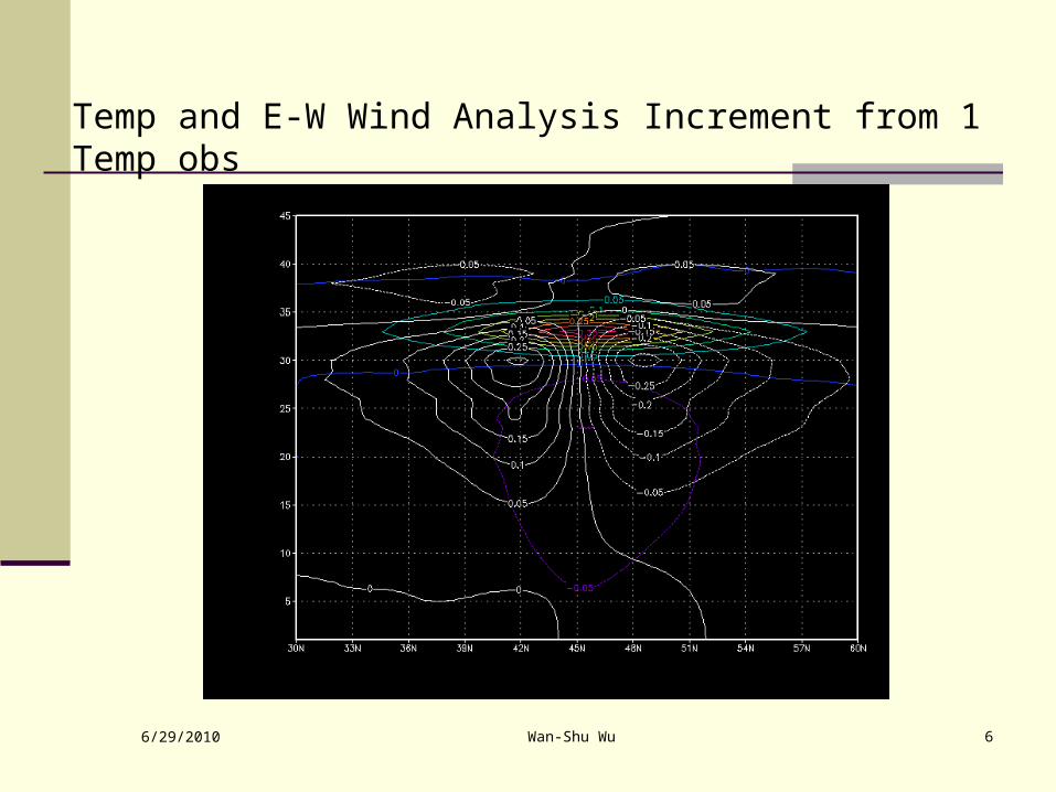
Temp and E-W Wind Analysis Increment from 1 Temp obs
6/29/2010 Wan-Shu Wu 7
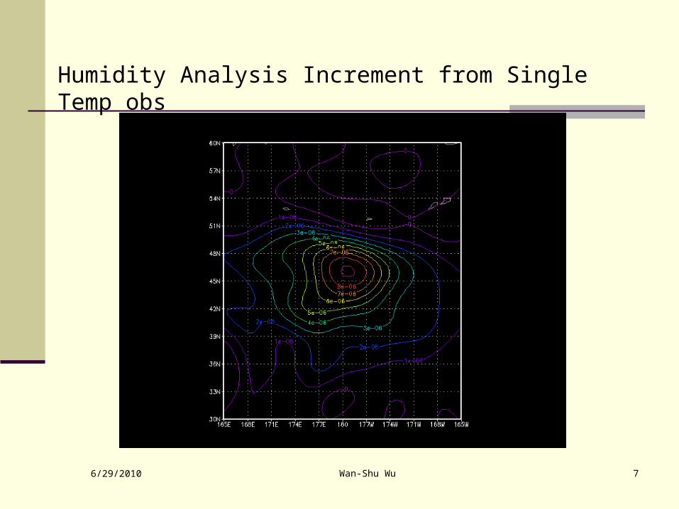
Humidity Analysis Increment from Single Temp obs
6/29/2010 Wan-Shu Wu 8
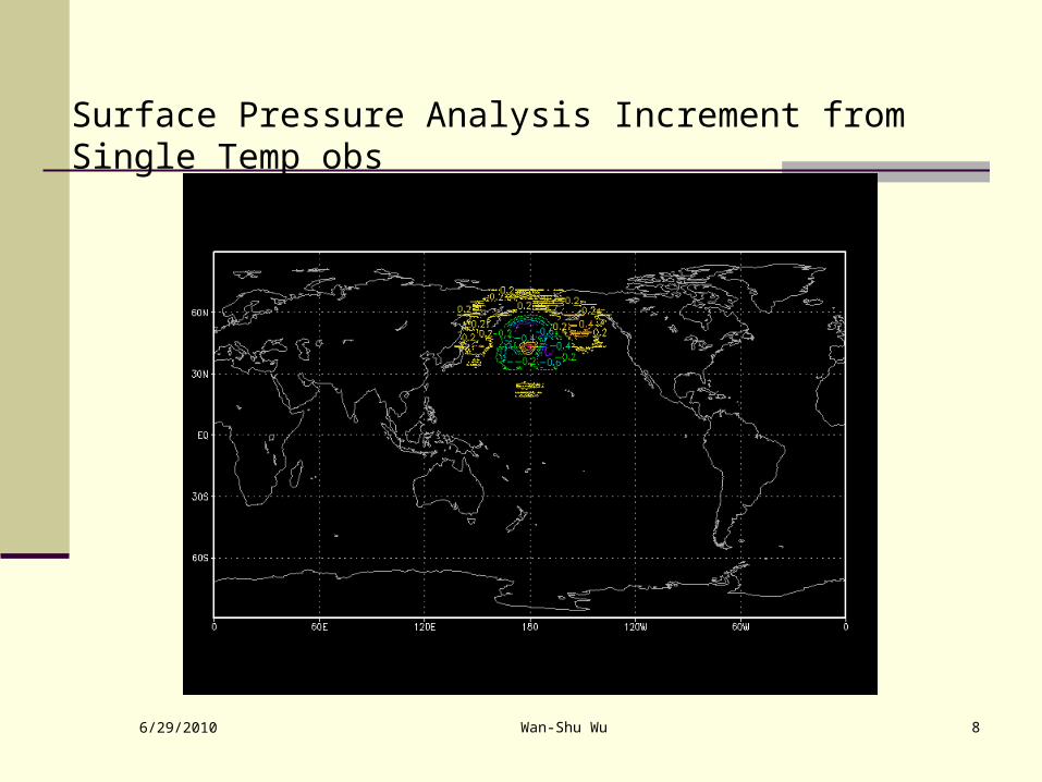
Surface Pressure Analysis Increment from Single Temp obs

6/29/2010 Wan-Shu Wu 9
Multivariate relation
Balanced part of the temperature is defined by
Tb = G where G is an empirical matrix that projects increments of stream function at one level to a vertical profile of balanced part of temperature increments. G is latitude dependent.
Balanced part of the velocity potential is defined as
b = c where coefficient c is function of latitude and height.
Balanced part of the surface pressure increment is defined as
Pb = W where matrix W integrates the appropriate contribution of the stream function from each level.
6/29/2010 Wan-Shu Wu 10
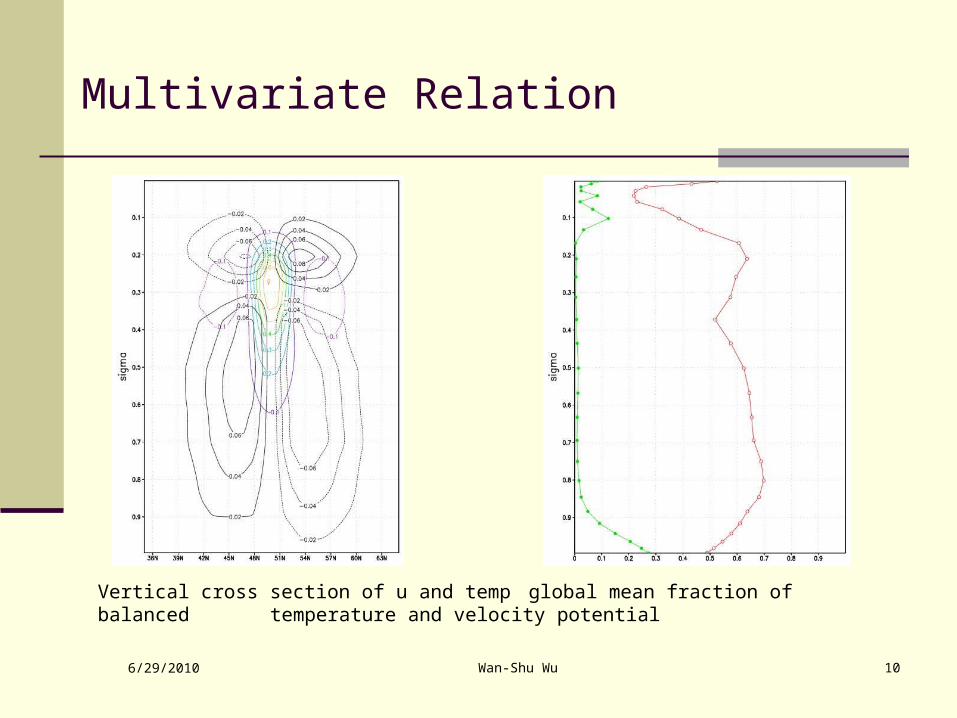
Multivariate Relation
Vertical cross section of u and temp global mean fraction of balanced temperature and velocity potential

6/29/2010 Wan-Shu Wu 11
Control Variable and Error Variances
Normalized relative humidity (qoption=2)
RH / RHb) = RHb ( P/Pb + q /qb - T /b )where
(RHb) : standard deviation of background error as function of RHb
b : - 1 / d(RH)/d(T)
multivariate relation with Temp and P
*Holm et al.(2002) ECMWF Tech Memo
6/29/2010 Wan-Shu Wu 12
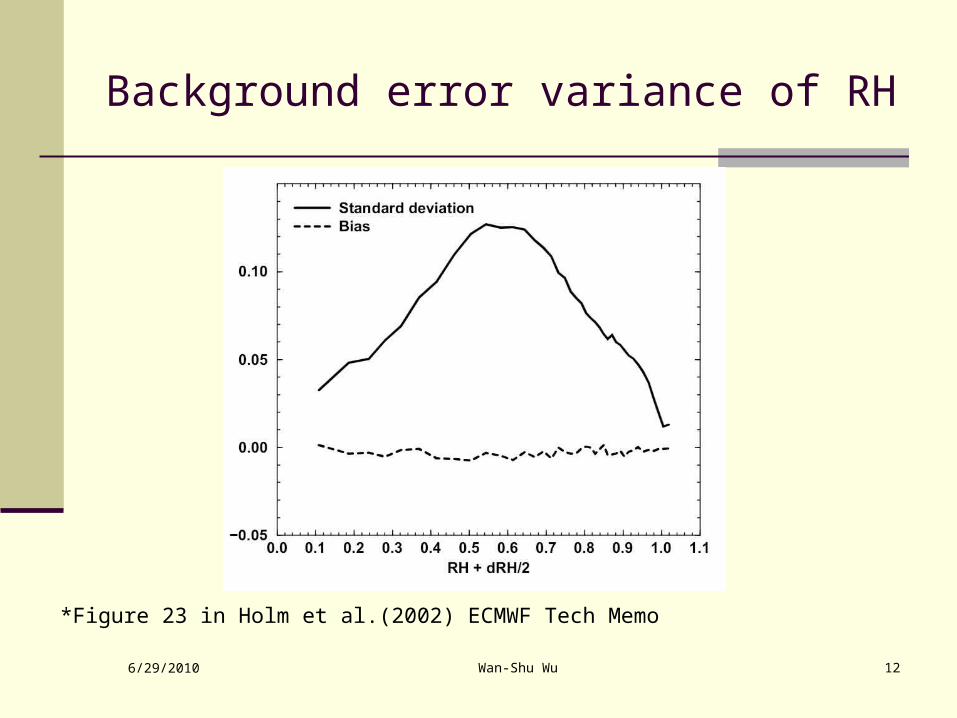
Background error variance of RH
*Figure 23 in Holm et al.(2002) ECMWF Tech Memo

6/29/2010 Wan-Shu Wu 13
Control Variables and Model Vaiables
U (left) and v (right) increments at sigma level 0.267, of a 1 m/s westerly wind observational residual at 50N and 330 E at 250 mb.
6/29/2010 Wan-Shu Wu 14
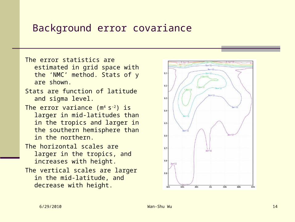
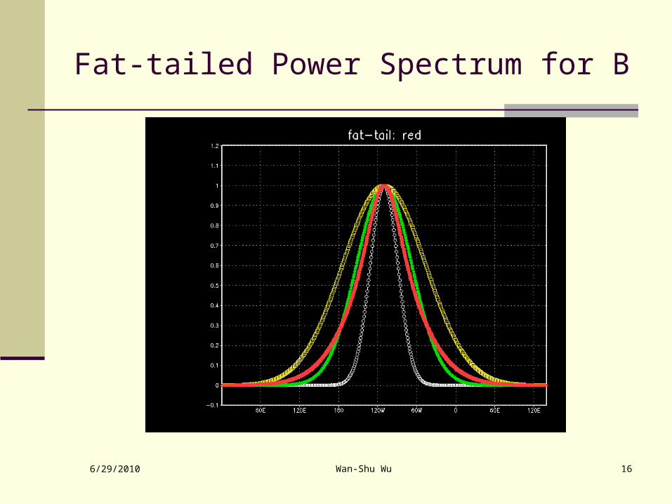
Background error covariance
The error statistics are estimated in grid space with the ‘NMC’ method. Stats of y are shown.
Stats are function of latitude and sigma level.
The error variance (m4 s-2) is larger in mid-latitudes than in the tropics and larger in the southern hemisphere than in the northern.
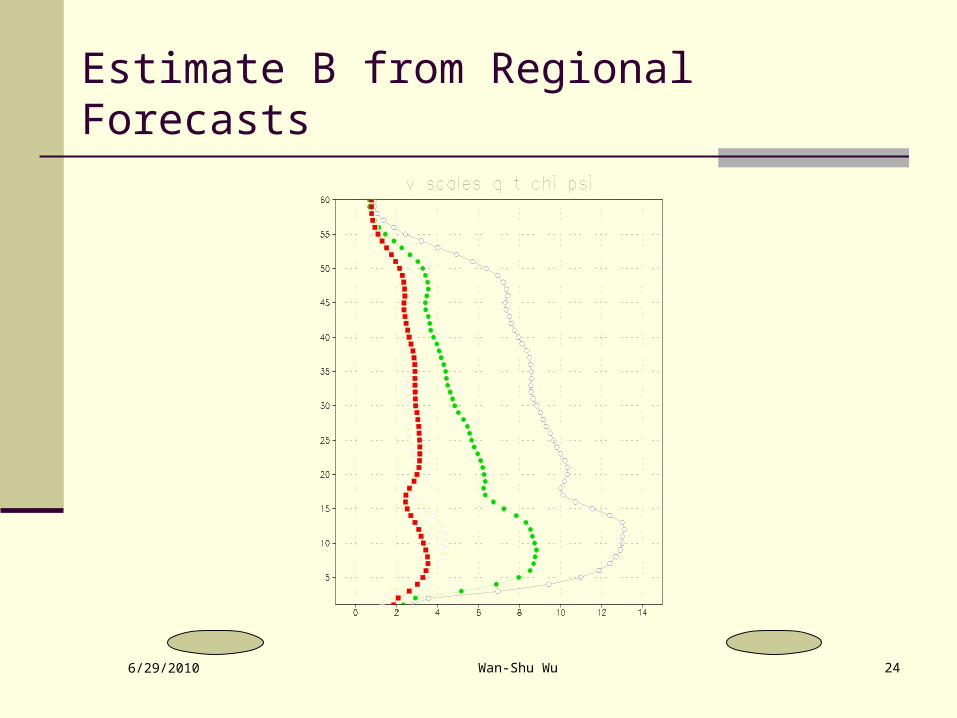
The horizontal scales are larger in the tropics, and increases with height.
The vertical scales are larger in the mid-latitude, and decrease with height.

6/29/2010 Wan-Shu Wu 15
Background error covariance
Horizontal scales in units of 100km vertical scale in units of vertical grid
6/29/2010 Wan-Shu Wu 16
Fat-tailed Power Spectrum for B

6/29/2010 Wan-Shu Wu 17
Fat-tailed Power Spectrum
Psfc increments with single homogeneous
recursive filter. (scale C) Cross validation
6/29/2010 Wan-Shu Wu 18
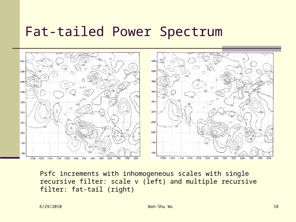
Fat-tailed Power Spectrum
Psfc increments with inhomogeneous scales with single recursive filter: scale v (left) and multiple recursive filter: fat-tail (right)
6/29/2010 Wan-Shu Wu 19
Estimate Background Error
NMC methodtime differences of forecasts (48-24hr)Basic assumption: linear error growth with time
Ensemble methodensemble differences of forecastsBasic assumption: ensemble represents real spread
Conventional methoddifferences of forecasts and obsdifficulties: obs coverage, multivariate…
6/29/2010 Wan-Shu Wu 20
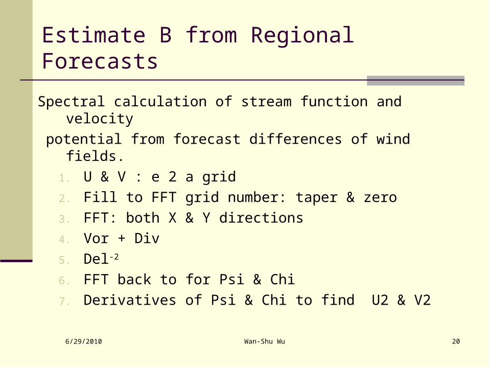
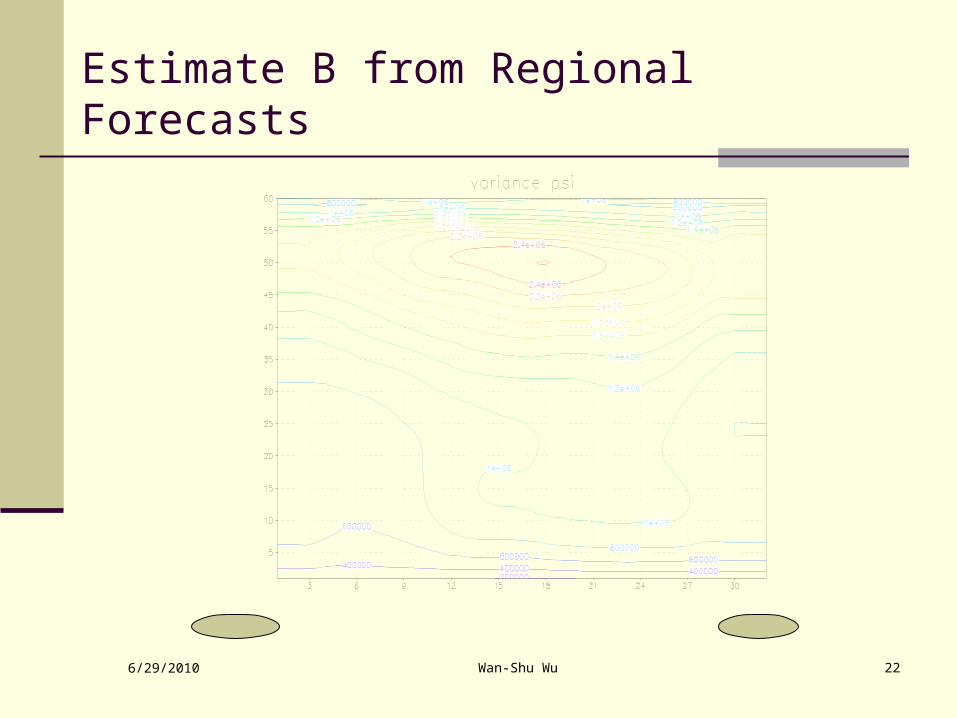
Estimate B from Regional Forecasts
Spectral calculation of stream function and velocity
potential from forecast differences of wind fields.
1. U & V : e 2 a grid
2. Fill to FFT grid number: taper & zero
3. FFT: both X & Y directions
4. Vor + Div
5. Del-2
6. FFT back to for Psi & Chi
7. Derivatives of Psi & Chi to find U2 & V2
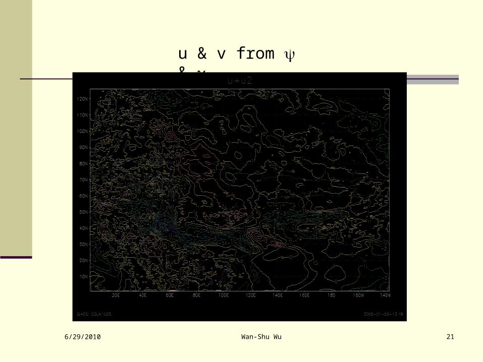
6/29/2010 Wan-Shu Wu 21
u & v from &
6/29/2010 Wan-Shu Wu 22
Estimate B from Regional Forecasts

6/29/2010 Wan-Shu Wu 23
Estimate B from Regional Forecasts
6/29/2010 Wan-Shu Wu 24
Estimate B from Regional Forecasts

6/29/2010 Wan-Shu Wu 25
Tuning Background Parameters
berror=$FIXnam/nam_glb_berror.f77
&BKGERRas=0.28,0.28,0.3,0.7,0.1,0.1,1.0,1.0,hzscl=0.373,0.746,1.50,vs=0.6,
(Note that hzscl and vs apply to all variables)
Q: How to find out definitions of “as”?A: GSI code
( grep “as(4)” *90 to find in prewgt_reg.f90 )

6/29/2010 Wan-Shu Wu 26
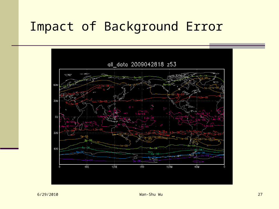
Impact of Background Error
6/29/2010 Wan-Shu Wu 27
Impact of Background Error

6/29/2010 Wan-Shu Wu 28
B adjustment ex2: Analysis increments of ozone
6/29/2010 Wan-Shu Wu 29
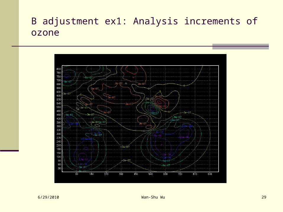
B adjustment ex1: Analysis increments of ozone
6/29/2010 Wan-Shu Wu 30
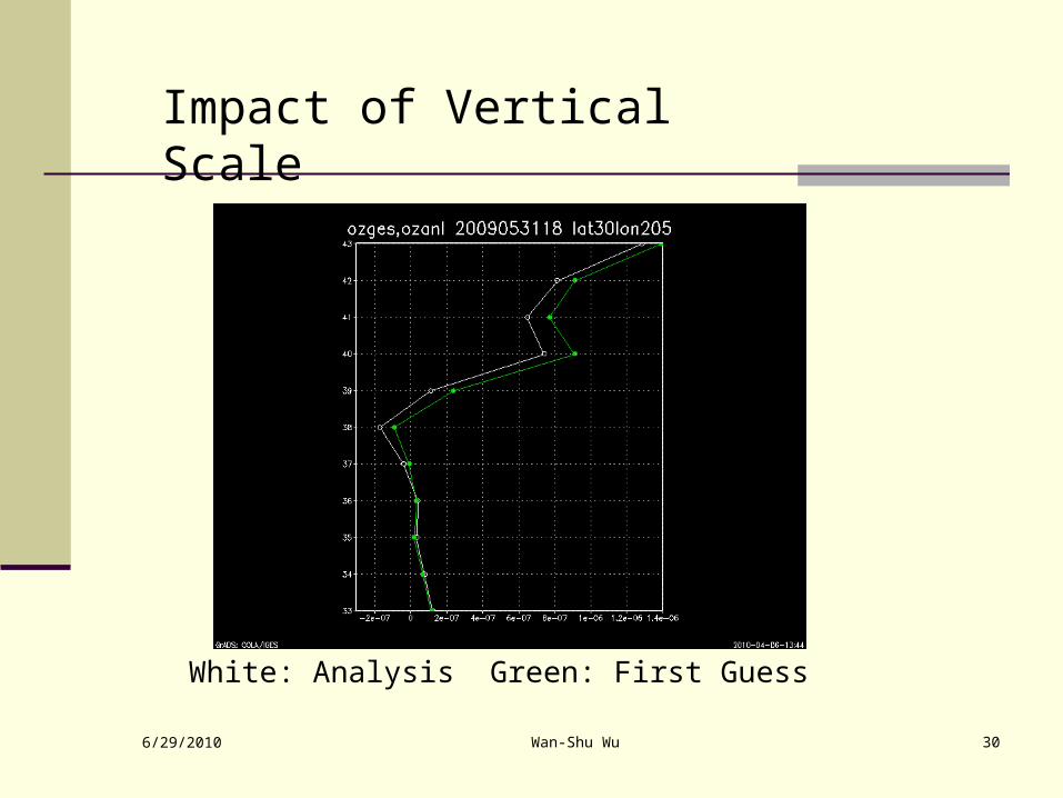
Impact of Vertical Scale
White: Analysis Green: First Guess

6/29/2010 Wan-Shu Wu 31
Impact of Vertical Scale
6/29/2010 Wan-Shu Wu 32
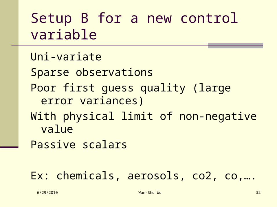
Setup B for a new control variable
Uni-variate
Sparse observations
Poor first guess quality (large error variances)
With physical limit of non-negative value
Passive scalars
Ex: chemicals, aerosols, co2, co,….
6/29/2010 Wan-Shu Wu 33
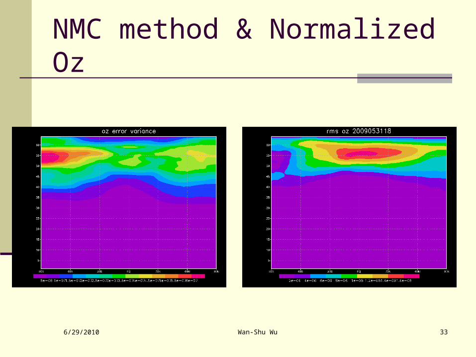
NMC method & Normalized Oz
6/29/2010 Wan-Shu Wu 34
Background error and their estimation
1. Multivariate relation
2. Background error covariance
3. Covariance with fat-tailed power spectrum
4. Estimate background error
6/29/2010 Wan-Shu Wu 35
Observational Error
Conventional adjustmentsAdaptive Tuning
6/29/2010 Wan-Shu Wu 36
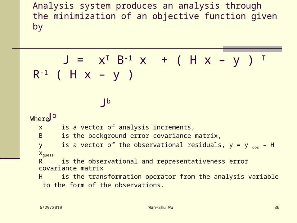
Analysis system produces an analysis through the minimization of an objective function given by
J = xT B-1 x + ( H x – y ) T R-1 ( H x – y )
Jb Jo
Wherex is a vector of analysis increments,B is the background error covariance matrix,
y is a vector of the observational residuals, y = y obs – H xguess
R is the observational and representativeness error covariance matrixH is the transformation operator from the analysis variable
to the form of the observations.
6/29/2010 Wan-Shu Wu 37
No method is optimal; There’ll be issues to solve and subjective tuning, smoothing, and averaging.
Ex: 1) background error
Ex: 2) ob error tune In a semi-operational system, tune B variances so that the
analysis penalties are about half of original penalties; including the scale effects.
Tune Oberror’s so that they are about the same as guess fit to data
Discussions
6/29/2010 Wan-Shu Wu 38
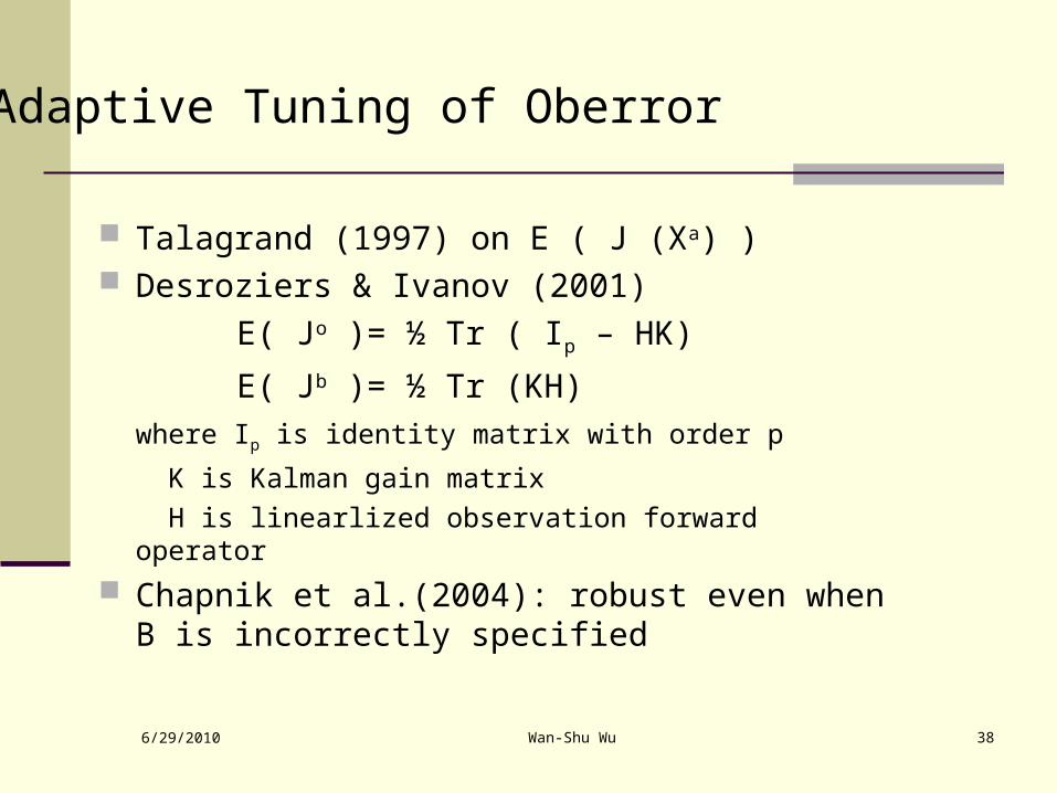
Talagrand (1997) on E ( J (Xa) ) Desroziers & Ivanov (2001)
E( Jo )= ½ Tr ( Ip – HK)
E( Jb )= ½ Tr (KH)
where Ip is identity matrix with order p
K is Kalman gain matrix
H is linearlized observation forward operator
Chapnik et al.(2004): robust even when B is incorrectly specified
Adaptive Tuning of Oberror
6/29/2010 Wan-Shu Wu 39
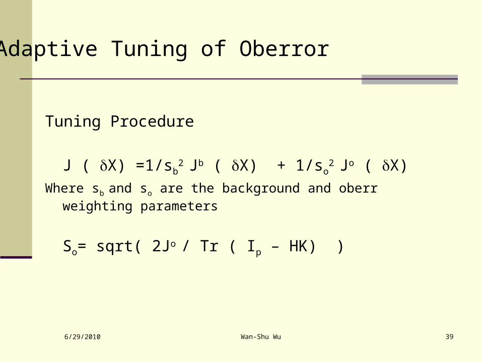
Tuning Procedure
J ( X) =1/sb2 Jb ( X) + 1/so
2 Jo ( X)
Where sb and so are the background and oberr weighting parameters
So= sqrt( 2Jo / Tr ( Ip – HK) )
Adaptive Tuning of Oberror

6/29/2010 Wan-Shu Wu 40
Analysis system produces an analysis through the minimization of an objective function given by
J = xT B-1 x + ( H x – y ) T R-1 ( H x – y )
Jb Jo
Wherex is a vector of analysis increments,B is the background error covariance matrix,
y is a vector of the observational residuals, y = y obs – H xguess
R is the observational and representativeness error covariance matrixH is the transformation operator from the analysis variable
to the form of the observations.

6/29/2010 Wan-Shu Wu 41
Tr ( Ip – HK) = Nobs -
( R-1/2 H Xa(y+R1/2+ R-1/2 H Xa(ywhere is random number with standard Gaussian distribution (mean: 0;variance:1 )
2 outer iterations each produces an analysis;
output new error table
Consecutive jobs show the method converged
Sum = (1-so)2
Randomized estimation of Tr (HK)

6/29/2010 Wan-Shu Wu 42
So for each ob type
So function of height (pressure)
rawinsonde, aircft, aircar, profiler winds, dropsonde, satwind…
So constant with height
ship, synoptic, metar, bogus, ssm/I, ers speed, aircft wind, aircar wind…
The setup can be changed in penal.f90

6/29/2010 Wan-Shu Wu 43
Turn on adaptive tuning of Oberr
1) &SETUPoberror_tune=.true.
2) If Global mode:&OBSQCoberrflg=.true.
(Regional mode: oberrflg=.true. is default)(find in file stdout: GSIMOD: ***WARNING*** reset oberrflg= T)
Note: GSI does not produce a valid analysis under the setup
6/29/2010 Wan-Shu Wu 44
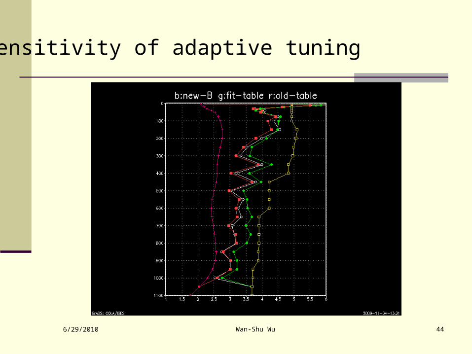
Sensitivity of adaptive tuning
6/29/2010 Wan-Shu Wu 45
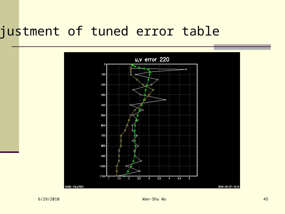
Adjustment of tuned error table
6/29/2010 Wan-Shu Wu 46
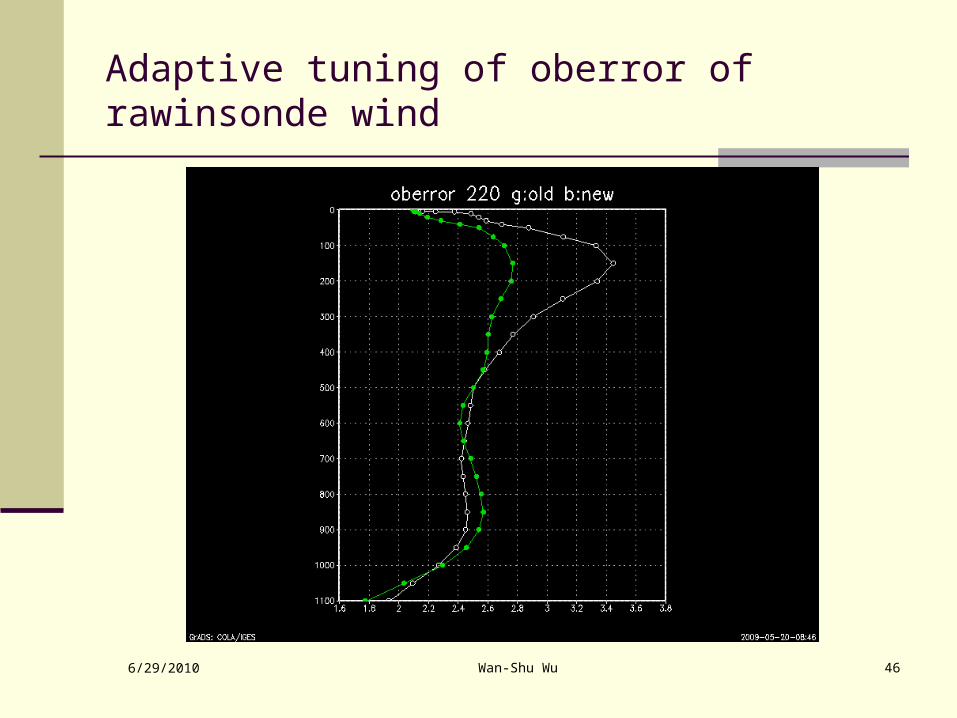
Adaptive tuning of oberror of rawinsonde wind
6/29/2010 Wan-Shu Wu 47
1) Can the tuning parameters of background error be changed with different outer loop?
A: No, they should not be changed. ( solving for the same original problem)
2) Why more than one outer loop?
A: To account for the nonlinear effect of the observational forward operator.
Questions on B and outer loop
6/29/2010 Wan-Shu Wu 48
Working code = answers to most questions
with print and plot Plot to check changes
Good Luck on Using GSI!
Suggestions