GSAS 2019 Operations Assessment & Guidelines Manual - For ...

ICESat (GLAS) Science Processing
Software Document Series
Volume #GSAS Detailed Design DocumentVersion 3.0
Jeffrey Lee/Raytheon ITSSObservational Science BranchLaboratory for Hydrospheric ProcessesNASA/GSFC Wallops Flight FacilityWallops Island, Virginia 23337
October 2002
ICESat Contacts:
Bob E. Schutz, GLAS Science Team LeaderUniversity of Texas Center for Space ResearchAustin, Texas 78759-5321
David W. Hancock III, Science Software Development LeaderNASA/GSFC Wallops Flight FacilityWallops Island, Virginia 23337
H. Jay Zwally, ICESat Project ScientistNASA Goddard Space Flight CenterGreenbelt, Maryland 20771


Foreword
This document describes the detailed design of GLAS Science Algorithm Software.
The GEOSCIENCE LASER ALTIMETER SYSTEM (GLAS) is a part of the EOS pro-gram. This laser altimetry mission will be carried on the spacecraft designated EOS ICESat (Ice, Cloud and Land Elevation Satellite). The GLAS laser is a frequency-dou-bled, cavity-pumped, solid state Nd:YAG laser.
This document was prepared by the Observational Science Branch at NASA GSFC/WFF, Wallops Island, VA, in support of B. E. Schutz, GLAS Science Team Leader for the GLAS Investigation. This work was performed under the direction of David W. Hancock, III, who may be contacted at (757) 824-1238, [email protected] (e-mail), or (757) 824-1036 (FAX).
The following GLAS Team members contributed to the creation of this document:
Raytheon/Kristine Barbieri
Raytheon/Suneel Bhardwaj
Raytheon/Anita Brenner
972/David W. Hancock, III
Raytheon/Peggy Jester
Raytheon/Steve McLaughlin
Raytheon/Carol Purdy
Raytheon/Lee Anne Roberts
October 2002 Page iii Version 3.0

GSAS Detailed Design Document Foreword
Version 3.0 Page iv October 2002

Table of Contents
Foreword . . . . . . . . . . . . . . . . . . . . . . . . . . . . . . . . . . . . . . . . . . . . . . . . . . . . . . . . . . iiiTable of Contents . . . . . . . . . . . . . . . . . . . . . . . . . . . . . . . . . . . . . . . . . . . . . . . . . . . . vList of Figures. . . . . . . . . . . . . . . . . . . . . . . . . . . . . . . . . . . . . . . . . . . . . . . . . . . . . . . ixList of Tables . . . . . . . . . . . . . . . . . . . . . . . . . . . . . . . . . . . . . . . . . . . . . . . . . . . . . . .xi
Section 1 Introduction1.1 Identification of Document . . . . . . . . . . . . . . . . . . . . . . . . . . . . . . . 1-11.2 Scope of Document . . . . . . . . . . . . . . . . . . . . . . . . . . . . . . . . . . . . . 1-11.3 Purpose and Objectives of Document . . . . . . . . . . . . . . . . . . . . . . . 1-11.4 Document Status and Schedule . . . . . . . . . . . . . . . . . . . . . . . . . . . 1-11.5 Document Organization . . . . . . . . . . . . . . . . . . . . . . . . . . . . . . . . . 1-11.6 Document Change History . . . . . . . . . . . . . . . . . . . . . . . . . . . . . . . 1-2
Section 2 Related Documentation2.1 Parent Documents. . . . . . . . . . . . . . . . . . . . . . . . . . . . . . . . . . . . . . 2-12.2 Applicable Documents. . . . . . . . . . . . . . . . . . . . . . . . . . . . . . . . . . . 2-12.3 Information Documents . . . . . . . . . . . . . . . . . . . . . . . . . . . . . . . . . 2-2
Section 3 Design Issues3.1 Requirements. . . . . . . . . . . . . . . . . . . . . . . . . . . . . . . . . . . . . . . . . . 3-13.2 Single vs. Multiple Executables . . . . . . . . . . . . . . . . . . . . . . . . . . . 3-13.3 Software Reuse . . . . . . . . . . . . . . . . . . . . . . . . . . . . . . . . . . . . . . . . 3-23.4 I/O and Unit Conversion . . . . . . . . . . . . . . . . . . . . . . . . . . . . . . . . . 3-23.5 Reprocessing and Pass-Thrus. . . . . . . . . . . . . . . . . . . . . . . . . . . . . 3-23.6 Data Buffering. . . . . . . . . . . . . . . . . . . . . . . . . . . . . . . . . . . . . . . . . 3-3
Section 4 Design Overview4.1 GSAS Design Overview. . . . . . . . . . . . . . . . . . . . . . . . . . . . . . . . . . 4-14.2 PGEs . . . . . . . . . . . . . . . . . . . . . . . . . . . . . . . . . . . . . . . . . . . . . . . . 4-14.3 Files . . . . . . . . . . . . . . . . . . . . . . . . . . . . . . . . . . . . . . . . . . . . . . . . . 4-34.4 Science Algorithms . . . . . . . . . . . . . . . . . . . . . . . . . . . . . . . . . . . . . 4-34.5 Utilities . . . . . . . . . . . . . . . . . . . . . . . . . . . . . . . . . . . . . . . . . . . . . . 4-3
Section 5 Foundation Libraries5.1 The Platform Library (platform_lib) . . . . . . . . . . . . . . . . . . . . . . . 5-15.2 The Control Library (cntrl_lib) . . . . . . . . . . . . . . . . . . . . . . . . . . . . 5-25.3 The Error Library (err_lib) . . . . . . . . . . . . . . . . . . . . . . . . . . . . . . . 5-35.4 The Math Library (math_lib) . . . . . . . . . . . . . . . . . . . . . . . . . . . . . 5-45.5 The Ancillary Library (anc_lib) . . . . . . . . . . . . . . . . . . . . . . . . . . . 5-45.6 The File Library (file_lib) . . . . . . . . . . . . . . . . . . . . . . . . . . . . . . . . 5-65.7 The Time Library (time_lib) . . . . . . . . . . . . . . . . . . . . . . . . . . . . . . 5-65.8 The Product Library (prod_lib). . . . . . . . . . . . . . . . . . . . . . . . . . . . 5-75.9 The Exec Library (exec_lib) . . . . . . . . . . . . . . . . . . . . . . . . . . . . . . 5-8
October 2002 Page v Version 3.0

GSAS Detailed Design Document Table of Contents
Section 6 Common Functionality6.1 Control File Parsing . . . . . . . . . . . . . . . . . . . . . . . . . . . . . . . . . . . . 6-16.2 ANC07 Constants Files . . . . . . . . . . . . . . . . . . . . . . . . . . . . . . . . . 6-56.3 Invalid Values and Error/Status Reporting . . . . . . . . . . . . . . . . . 6-66.4 ANC06 Metadata/Log File . . . . . . . . . . . . . . . . . . . . . . . . . . . . . . . 6-96.5 Product Internal Data Storage, Conversion and I/O . . . . . . . . . . 6-96.6 Product Headers . . . . . . . . . . . . . . . . . . . . . . . . . . . . . . . . . . . . . . 6-126.7 Summary. . . . . . . . . . . . . . . . . . . . . . . . . . . . . . . . . . . . . . . . . . . . 6-13
Section 7 GSAS Core PGEs7.1 Function . . . . . . . . . . . . . . . . . . . . . . . . . . . . . . . . . . . . . . . . . . . . . 7-17.2 Requirements . . . . . . . . . . . . . . . . . . . . . . . . . . . . . . . . . . . . . . . . . 7-17.3 Approach . . . . . . . . . . . . . . . . . . . . . . . . . . . . . . . . . . . . . . . . . . . . . 7-17.4 Design . . . . . . . . . . . . . . . . . . . . . . . . . . . . . . . . . . . . . . . . . . . . . . . 7-2
Section 8 GLAS_L0proc8.1 Overview . . . . . . . . . . . . . . . . . . . . . . . . . . . . . . . . . . . . . . . . . . . . . 8-18.2 Function . . . . . . . . . . . . . . . . . . . . . . . . . . . . . . . . . . . . . . . . . . . . . 8-18.3 Approach . . . . . . . . . . . . . . . . . . . . . . . . . . . . . . . . . . . . . . . . . . . . . 8-28.4 Input and Output Files. . . . . . . . . . . . . . . . . . . . . . . . . . . . . . . . . . 8-28.5 Design . . . . . . . . . . . . . . . . . . . . . . . . . . . . . . . . . . . . . . . . . . . . . . . 8-7
Section 9 GLAS_L1A9.1 Overview . . . . . . . . . . . . . . . . . . . . . . . . . . . . . . . . . . . . . . . . . . . . . 9-19.2 Function . . . . . . . . . . . . . . . . . . . . . . . . . . . . . . . . . . . . . . . . . . . . . 9-19.3 Design Approach. . . . . . . . . . . . . . . . . . . . . . . . . . . . . . . . . . . . . . . 9-19.4 Input and Output Files. . . . . . . . . . . . . . . . . . . . . . . . . . . . . . . . . . 9-29.5 GLAS_L1A PGE . . . . . . . . . . . . . . . . . . . . . . . . . . . . . . . . . . . . . . . 9-29.6 L1A Manager (L1A_Mgr) . . . . . . . . . . . . . . . . . . . . . . . . . . . . . . . . 9-49.7 PGE/Manager Implementation Details. . . . . . . . . . . . . . . . . . . . . 9-69.8 L1A_Subsystem . . . . . . . . . . . . . . . . . . . . . . . . . . . . . . . . . . . . . . . 9-8
Section 10 GLAS_Alt10.1 Function . . . . . . . . . . . . . . . . . . . . . . . . . . . . . . . . . . . . . . . . . . . . 10-110.2 Design Approach. . . . . . . . . . . . . . . . . . . . . . . . . . . . . . . . . . . . . . 10-110.3 Input and Output Files. . . . . . . . . . . . . . . . . . . . . . . . . . . . . . . . . 10-110.4 GLAS_Alt . . . . . . . . . . . . . . . . . . . . . . . . . . . . . . . . . . . . . . . . . . . 10-410.5 Waveform Manager (WF_Mgr) . . . . . . . . . . . . . . . . . . . . . . . . . . 10-510.6 Elevation Manager (Elev_Mgr) . . . . . . . . . . . . . . . . . . . . . . . . . . 10-810.7 PGE/Manager Implementation Details. . . . . . . . . . . . . . . . . . . . 10-910.8 WF_Subsystem . . . . . . . . . . . . . . . . . . . . . . . . . . . . . . . . . . . . . . 10-2010.9 Elev_Subsystem . . . . . . . . . . . . . . . . . . . . . . . . . . . . . . . . . . . . . 10-37
Section 11 GLAS_Atm11.1 Overview . . . . . . . . . . . . . . . . . . . . . . . . . . . . . . . . . . . . . . . . . . . . 11-111.2 Function . . . . . . . . . . . . . . . . . . . . . . . . . . . . . . . . . . . . . . . . . . . . 11-111.3 Design Approach. . . . . . . . . . . . . . . . . . . . . . . . . . . . . . . . . . . . . . 11-1
Version 3.0 Page vi October 2002

Table of Contents GSAS Detailed Design Document
11.4 Input and Output Files . . . . . . . . . . . . . . . . . . . . . . . . . . . . . . . . . 11-211.5 Functions . . . . . . . . . . . . . . . . . . . . . . . . . . . . . . . . . . . . . . . . . . . . 11-411.6 Atm_Subsystem. . . . . . . . . . . . . . . . . . . . . . . . . . . . . . . . . . . . . . . 11-9
Section 12 GLAS_Reader12.1 Function . . . . . . . . . . . . . . . . . . . . . . . . . . . . . . . . . . . . . . . . . . . . . 12-112.2 Design Approach . . . . . . . . . . . . . . . . . . . . . . . . . . . . . . . . . . . . . . 12-112.3 Input and Output Files . . . . . . . . . . . . . . . . . . . . . . . . . . . . . . . . . 12-112.4 GLAS_Reader . . . . . . . . . . . . . . . . . . . . . . . . . . . . . . . . . . . . . . . . 12-3
Section 13 met_util13.1 Overview . . . . . . . . . . . . . . . . . . . . . . . . . . . . . . . . . . . . . . . . . . . . 13-113.2 Function . . . . . . . . . . . . . . . . . . . . . . . . . . . . . . . . . . . . . . . . . . . . . 13-113.3 Design Approach . . . . . . . . . . . . . . . . . . . . . . . . . . . . . . . . . . . . . . 13-113.4 Input and Output Files . . . . . . . . . . . . . . . . . . . . . . . . . . . . . . . . . 13-113.5 Functions . . . . . . . . . . . . . . . . . . . . . . . . . . . . . . . . . . . . . . . . . . . . 13-113.6 Functional Overview . . . . . . . . . . . . . . . . . . . . . . . . . . . . . . . . . . . 13-2
Section 14 reforbit_util14.1 Overview . . . . . . . . . . . . . . . . . . . . . . . . . . . . . . . . . . . . . . . . . . . . 14-114.2 Function . . . . . . . . . . . . . . . . . . . . . . . . . . . . . . . . . . . . . . . . . . . . . 14-114.3 Design Approach . . . . . . . . . . . . . . . . . . . . . . . . . . . . . . . . . . . . . . 14-114.4 Input and Output Files . . . . . . . . . . . . . . . . . . . . . . . . . . . . . . . . . 14-114.5 Functions . . . . . . . . . . . . . . . . . . . . . . . . . . . . . . . . . . . . . . . . . . . . 14-114.6 Functional Overview . . . . . . . . . . . . . . . . . . . . . . . . . . . . . . . . . . . 14-2
Section 15 createGran_util15.1 Overview . . . . . . . . . . . . . . . . . . . . . . . . . . . . . . . . . . . . . . . . . . . . 15-115.2 Function . . . . . . . . . . . . . . . . . . . . . . . . . . . . . . . . . . . . . . . . . . . . . 15-115.3 Design Approach . . . . . . . . . . . . . . . . . . . . . . . . . . . . . . . . . . . . . . 15-115.4 Input and Output Files . . . . . . . . . . . . . . . . . . . . . . . . . . . . . . . . . 15-415.5 Functions . . . . . . . . . . . . . . . . . . . . . . . . . . . . . . . . . . . . . . . . . . . . 15-515.6 Functional Overview . . . . . . . . . . . . . . . . . . . . . . . . . . . . . . . . . . . 15-5
Section 16 atm_anc16.1 Overview . . . . . . . . . . . . . . . . . . . . . . . . . . . . . . . . . . . . . . . . . . . . 16-116.2 Function . . . . . . . . . . . . . . . . . . . . . . . . . . . . . . . . . . . . . . . . . . . . . 16-116.3 Design Approach . . . . . . . . . . . . . . . . . . . . . . . . . . . . . . . . . . . . . . 16-116.4 Input and Output Files . . . . . . . . . . . . . . . . . . . . . . . . . . . . . . . . . 16-116.5 Functions . . . . . . . . . . . . . . . . . . . . . . . . . . . . . . . . . . . . . . . . . . . . 16-216.6 Functional Overview of Calibration Modules . . . . . . . . . . . . . . . 16-2
Section 17 GLAS_Meta17.1 Function . . . . . . . . . . . . . . . . . . . . . . . . . . . . . . . . . . . . . . . . . . . . . 17-117.2 Design Approach . . . . . . . . . . . . . . . . . . . . . . . . . . . . . . . . . . . . . . 17-117.3 Input and Output Files . . . . . . . . . . . . . . . . . . . . . . . . . . . . . . . . . 17-117.4 GLAS_Meta . . . . . . . . . . . . . . . . . . . . . . . . . . . . . . . . . . . . . . . . . . 17-3
October 2002 Page vii Version 3.0

GSAS Detailed Design Document Table of Contents
Section 18 GLAS_APID18.1 Function . . . . . . . . . . . . . . . . . . . . . . . . . . . . . . . . . . . . . . . . . . . . 18-118.2 Design Approach. . . . . . . . . . . . . . . . . . . . . . . . . . . . . . . . . . . . . . 18-118.3 Input and Output Files. . . . . . . . . . . . . . . . . . . . . . . . . . . . . . . . . 18-118.4 GLAS_APID . . . . . . . . . . . . . . . . . . . . . . . . . . . . . . . . . . . . . . . . . 18-2
Appendix A Processing Scenarios
Appendix B Makefiles and LibrariesB.1 Compilation. . . . . . . . . . . . . . . . . . . . . . . . . . . . . . . . . . . . . . . . . . . B-1B.2 Using Libraries . . . . . . . . . . . . . . . . . . . . . . . . . . . . . . . . . . . . . . . . B-2B.3 Some Development Hints . . . . . . . . . . . . . . . . . . . . . . . . . . . . . . . . B-2B.4 Makefile Details . . . . . . . . . . . . . . . . . . . . . . . . . . . . . . . . . . . . . . . B-3B.5 Types of Makefiles . . . . . . . . . . . . . . . . . . . . . . . . . . . . . . . . . . . . . B-3B.6 A Sample Heavily-Commented Makefile . . . . . . . . . . . . . . . . . . . B-4
Abbreviations & Acronyms. . . . . . . . . . . . . . . . . . . . . . . . . . . . . . . . . . . . . . . . . . AB-1Glossary. . . . . . . . . . . . . . . . . . . . . . . . . . . . . . . . . . . . . . . . . . . . . . . . . . . . . . . . GL-1
Version 3.0 Page viii October 2002

List of Figures
Figure 1-1 I-SIPS Software Top-Level Decomposition . . . . . . . . . . . . . . . . . . . 1-2
Figure 4-1 GSAS Layers . . . . . . . . . . . . . . . . . . . . . . . . . . . . . . . . . . . . . . . . . . . . 4-1
Figure 4-2 Simplified GSAS Data Flow Diagram . . . . . . . . . . . . . . . . . . . . . . . 4-2
Figure 6-1 Error Ancillary File Format . . . . . . . . . . . . . . . . . . . . . . . . . . . . . . . . 6-7
Figure 7-1 Top-Level Structure Chart . . . . . . . . . . . . . . . . . . . . . . . . . . . . . . . . . 7-3
Figure 7-2 MainInit . . . . . . . . . . . . . . . . . . . . . . . . . . . . . . . . . . . . . . . . . . . . . . . . 7-4
Figure 7-3 GetControl . . . . . . . . . . . . . . . . . . . . . . . . . . . . . . . . . . . . . . . . . . . . . . 7-5
Figure 7-4 ReadData . . . . . . . . . . . . . . . . . . . . . . . . . . . . . . . . . . . . . . . . . . . . . . . 7-8
Figure 8-1 GLAS_L0proc Structure Chart . . . . . . . . . . . . . . . . . . . . . . . . . . . . . 8-8
Figure 9-1 GLAS_L1A Structure Chart. . . . . . . . . . . . . . . . . . . . . . . . . . . . . . . . 9-4
Figure 9-2 L1A_Mgr Structure Chart . . . . . . . . . . . . . . . . . . . . . . . . . . . . . . . . . 9-5
Figure 9-3 L1A Manager Flow Chart . . . . . . . . . . . . . . . . . . . . . . . . . . . . . . . . . 9-6
Figure 9-4 Level 1A Computations . . . . . . . . . . . . . . . . . . . . . . . . . . . . . . . . . . . 9-8
Figure 10-1 GLAS_Alt Structure Chart. . . . . . . . . . . . . . . . . . . . . . . . . . . . . . . . 10-5
Figure 10-2 WF_Mgr Structure Chart . . . . . . . . . . . . . . . . . . . . . . . . . . . . . . . . . 10-6
Figure 10-3 WF Manager Flowchart . . . . . . . . . . . . . . . . . . . . . . . . . . . . . . . . . . 10-7
Figure 10-4 Elev_Mgr Structure Chart . . . . . . . . . . . . . . . . . . . . . . . . . . . . . . . . 10-9
Figure 10-5 Elev_Mgr Flow Chart . . . . . . . . . . . . . . . . . . . . . . . . . . . . . . . . . . . 10-10
Figure 10-6 W_Assess . . . . . . . . . . . . . . . . . . . . . . . . . . . . . . . . . . . . . . . . . . . . . 10-21
Figure 10-7 Assess Waveform Sub-Processes . . . . . . . . . . . . . . . . . . . . . . . . . 10-24
Figure 10-8 W_FunctionalFt . . . . . . . . . . . . . . . . . . . . . . . . . . . . . . . . . . . . . . . . 10-27
Figure 10-9 W_FunctionalFt Subprocesses. . . . . . . . . . . . . . . . . . . . . . . . . . . . 10-28
Figure 10-10 WFMgr Structure Chart . . . . . . . . . . . . . . . . . . . . . . . . . . . . . . . . . 10-36
Figure 10-11 W_Assess Structure Chart . . . . . . . . . . . . . . . . . . . . . . . . . . . . . . . 10-36
Figure 10-12 W_FunctionalFt Structure Chart. . . . . . . . . . . . . . . . . . . . . . . . . . 10-37
Figure 10-13 Level 1B and 2 Elevation DFD . . . . . . . . . . . . . . . . . . . . . . . . . . . 10-38
Figure 10-14 Level 1B Elevation Computation DFD. . . . . . . . . . . . . . . . . . . . . 10-39
Figure 10-15 Tide Corrections Routines DFD . . . . . . . . . . . . . . . . . . . . . . . . . . 10-40
Figure 10-16 Calculate Level2 Elevations DFD . . . . . . . . . . . . . . . . . . . . . . . . . 10-41
Figure 10-17 Elevation Manager . . . . . . . . . . . . . . . . . . . . . . . . . . . . . . . . . . . . . 10-42
October 2002 Page ix Version 3.0

GSAS Detailed Design Document List of Figures
Figure 10-18 Calculate Level 2 Elevations Structure Chart . . . . . . . . . . . . . . . 10-45
Figure 10-19 Tide Correction Routines Structure Chart. . . . . . . . . . . . . . . . . . 10-46
Figure 10-20 GetGeoid Structure Chart . . . . . . . . . . . . . . . . . . . . . . . . . . . . . . . 10-46
Figure 10-21 Calculate Trop Corrections Structure Chart . . . . . . . . . . . . . . . . 10-47
Figure 11-1 GLAS_Atm Structure Chart . . . . . . . . . . . . . . . . . . . . . . . . . . . . . . 11-5
Figure 11-2 Atm_Mgr Structure Chart . . . . . . . . . . . . . . . . . . . . . . . . . . . . . . . . 11-6
Figure 11-3 ATM Manager - Part 1 . . . . . . . . . . . . . . . . . . . . . . . . . . . . . . . . . . . 11-7
Figure 11-4 ATM Manager - Part 2 . . . . . . . . . . . . . . . . . . . . . . . . . . . . . . . . . . . 11-8
Figure 11-5 Atmosphere Subsystem Processes . . . . . . . . . . . . . . . . . . . . . . . . 11-10
Figure 11-6 ATM L1B Calculate Calibration Coefficients, Profile Locations, and DEM Subprocesses. . . . . . . . . . . . . . . . . . . . . . . . . . . . . . . . . . 11-11
Figure 11-7 ATM L1B Backscatter Subprocesses. . . . . . . . . . . . . . . . . . . . . . . 11-12
Figure 11-8 ATM L1B QA Statistics and WriteATM Subprocesses . . . . . . . 11-13
Figure 11-9 ATM L1B QA Statistics and WriteATM Subprocesses . . . . . . . 11-14
Figure 11-10 ATM L2: Cloud / Aerosol Layer Heights Subprocesses. . . . . . 11-15
Figure 11-11 Atmosphere Subsystem: Optical Properties Subprocesses. . . . 11-16
Figure 11-12 ATM L2 QA Statistics and WriteATM Subprocesses . . . . . . . . 11-16
Figure 11-13 ATM Calibration Coefficient / Profile Location / DEM Modules. . . . . . . . . . . . . . . . . . . . . . . . . . . . . . . . . . . . . . . . . . 11-17
Figure 11-14 ATM Backscatter Modules. . . . . . . . . . . . . . . . . . . . . . . . . . . . . . . 11-17
Figure 11-15 ATM L1B QA Statistics / Write ATM Modules . . . . . . . . . . . . . 11-18
Figure 11-16 ATM 20 sec Buffering Module . . . . . . . . . . . . . . . . . . . . . . . . . . . 11-18
Figure 11-17 ATM Cloud / Aerosol Layer Heights Modules . . . . . . . . . . . . . 11-19
Figure 11-18 ATM Optical Properties Module . . . . . . . . . . . . . . . . . . . . . . . . . 11-19
Figure 11-19 L2 QA Statistics / Write ATM Modules . . . . . . . . . . . . . . . . . . . 11-20
Figure 13-1 Process Flow Diagram: Overall Process . . . . . . . . . . . . . . . . . . . . 13-3
Figure 13-2 Process Flow Diagram: Shell Script . . . . . . . . . . . . . . . . . . . . . . . . 13-4
Figure 14-1 Process Flow Diagram . . . . . . . . . . . . . . . . . . . . . . . . . . . . . . . . . . . 14-3
Figure 15-1 Process Flow Diagram . . . . . . . . . . . . . . . . . . . . . . . . . . . . . . . . . . . 15-6
Figure 16-1 Process Flow Diagram . . . . . . . . . . . . . . . . . . . . . . . . . . . . . . . . . . . 16-3
Version 3.0 Page x October 2002

List of Tables
Table 4-1 Subsystem, Libraries and Products . . . . . . . . . . . . . . . . . . . . . . . . . 4-3
Table 5-1 Library Inter-dependencies . . . . . . . . . . . . . . . . . . . . . . . . . . . . . . . . 5-1
Table 5-2 platform_lib Modules. . . . . . . . . . . . . . . . . . . . . . . . . . . . . . . . . . . . . 5-2
Table 5-3 cntrl_lib Modules . . . . . . . . . . . . . . . . . . . . . . . . . . . . . . . . . . . . . . . . 5-2
Table 5-4 err_lib Modules . . . . . . . . . . . . . . . . . . . . . . . . . . . . . . . . . . . . . . . . . . 5-3
Table 5-5 math_lib Modules . . . . . . . . . . . . . . . . . . . . . . . . . . . . . . . . . . . . . . . . 5-4
Table 5-6 anc_lib Modules . . . . . . . . . . . . . . . . . . . . . . . . . . . . . . . . . . . . . . . . . 5-4
Table 5-7 file_lib Modules. . . . . . . . . . . . . . . . . . . . . . . . . . . . . . . . . . . . . . . . . . 5-6
Table 5-8 time_lib Modules . . . . . . . . . . . . . . . . . . . . . . . . . . . . . . . . . . . . . . . . 5-7
Table 5-9 prod_lib Modules . . . . . . . . . . . . . . . . . . . . . . . . . . . . . . . . . . . . . . . . 5-7
Table 5-10 fexec_lib Modules . . . . . . . . . . . . . . . . . . . . . . . . . . . . . . . . . . . . . . . . 5-8
Table 6-1 Required Single-Instance Keywords . . . . . . . . . . . . . . . . . . . . . . . . 6-2
Table 6-2 Optional Multiple-Instance Keywords . . . . . . . . . . . . . . . . . . . . . . 6-2
Table 6-3 PASSID Control Line Elements. . . . . . . . . . . . . . . . . . . . . . . . . . . . . 6-2
Table 6-4 passid Field Description. . . . . . . . . . . . . . . . . . . . . . . . . . . . . . . . . . . 6-3
Table 6-5 File Segment and Version Fields. . . . . . . . . . . . . . . . . . . . . . . . . . . . 6-4
Table 6-6 Invalid Values . . . . . . . . . . . . . . . . . . . . . . . . . . . . . . . . . . . . . . . . . . . 6-6
Table 6-7 PGE Exit Status Codes . . . . . . . . . . . . . . . . . . . . . . . . . . . . . . . . . . . . 6-7
Table 6-9 Error Sections. . . . . . . . . . . . . . . . . . . . . . . . . . . . . . . . . . . . . . . . . . . . 6-8
Table 6-8 Error String Format. . . . . . . . . . . . . . . . . . . . . . . . . . . . . . . . . . . . . . . 6-8
Table 6-10 Error Severity Codes. . . . . . . . . . . . . . . . . . . . . . . . . . . . . . . . . . . . . . 6-9
Table 6-11 Product Module Functionality . . . . . . . . . . . . . . . . . . . . . . . . . . . . 6-10
Table 8-1 GLAS_L0proc Inputs . . . . . . . . . . . . . . . . . . . . . . . . . . . . . . . . . . . . . 8-2
Table 8-3 Supported APIDs . . . . . . . . . . . . . . . . . . . . . . . . . . . . . . . . . . . . . . . . 8-3
Table 8-2 GLAS_L0proc Outputs. . . . . . . . . . . . . . . . . . . . . . . . . . . . . . . . . . . . 8-3
Table 8-4 ANC33 Field Descriptions . . . . . . . . . . . . . . . . . . . . . . . . . . . . . . . . . 8-4
Table 8-6 ANC32 Format/Description . . . . . . . . . . . . . . . . . . . . . . . . . . . . . . . 8-6
Table 8-5 ANC29 Format/Description . . . . . . . . . . . . . . . . . . . . . . . . . . . . . . . 8-6
Table 9-1 GLAS_L1A Inputs. . . . . . . . . . . . . . . . . . . . . . . . . . . . . . . . . . . . . . . . 9-2
Table 9-2 GLAS_L1A Outputs . . . . . . . . . . . . . . . . . . . . . . . . . . . . . . . . . . . . . . 9-3
October 2002 Page xi Version 3.0

GSAS Detailed Design Document List of Tables
Table 10-1 GLAS_Alt Inputs. . . . . . . . . . . . . . . . . . . . . . . . . . . . . . . . . . . . . . . . 10-2
Table 10-2 GLAS_Alt Outputs . . . . . . . . . . . . . . . . . . . . . . . . . . . . . . . . . . . . . . 10-3
Table 11-1 GLAS_Atm Inputs . . . . . . . . . . . . . . . . . . . . . . . . . . . . . . . . . . . . . . 11-2
Table 11-2 GLAS_Atm Outputs . . . . . . . . . . . . . . . . . . . . . . . . . . . . . . . . . . . . . 11-3
Table 12-1 GLAS_Reader Inputs . . . . . . . . . . . . . . . . . . . . . . . . . . . . . . . . . . . . 12-1
Table 13-1 met_util Inputs . . . . . . . . . . . . . . . . . . . . . . . . . . . . . . . . . . . . . . . . . 13-2
Table 13-2 met_util Outputs . . . . . . . . . . . . . . . . . . . . . . . . . . . . . . . . . . . . . . . . 13-2
Table 14-1 createGran_util Inputs . . . . . . . . . . . . . . . . . . . . . . . . . . . . . . . . . . . 14-1
Table 14-2 createGran_util Outputs . . . . . . . . . . . . . . . . . . . . . . . . . . . . . . . . . 14-2
Table 15-1 createGran_util Inputs . . . . . . . . . . . . . . . . . . . . . . . . . . . . . . . . . . . 15-4
Table 15-2 createGran_util Outputs . . . . . . . . . . . . . . . . . . . . . . . . . . . . . . . . . 15-4
Table 16-1 atm_anc Inputs . . . . . . . . . . . . . . . . . . . . . . . . . . . . . . . . . . . . . . . . . 16-1
Table 16-2 atm_anc Outputs. . . . . . . . . . . . . . . . . . . . . . . . . . . . . . . . . . . . . . . . 16-2
Table 17-1 GLAS_Meta Inputs . . . . . . . . . . . . . . . . . . . . . . . . . . . . . . . . . . . . . . 17-1
Table 17-2 GLAS_Meta Outputs . . . . . . . . . . . . . . . . . . . . . . . . . . . . . . . . . . . . 17-2
Table 18-1 GLAS_APID Inputs . . . . . . . . . . . . . . . . . . . . . . . . . . . . . . . . . . . . . 18-1
Table 18-2 GLAS_APID Outputs . . . . . . . . . . . . . . . . . . . . . . . . . . . . . . . . . . . . 18-2
Table A-1 Reprocessing Scenarios . . . . . . . . . . . . . . . . . . . . . . . . . . . . . . . . . . . A-1
Version 3.0 Page xii October 2002

Section 1
Introduction
1.1 Identification of Document
This document is identified as the GLAS Science Algorithm Software (GSAS) Detailed Design Document. The unique document identification number within the GLAS Ground Data System numbering scheme is TBD. Successive editions of this document will be uniquely identified by the cover and page date marks.
1.2 Scope of Document
The GLAS I-SIPS Data Processing System, show in Figure 1-1, provides data process-ing and mission support for the Geoscience Laser Altimeter System (GLAS). I-SIPS is composed of two major software components - the GLAS Science Algorithm Soft-ware (GSAS) and the Scheduling and Data Management System (SDMS). GSAS pro-cesses Level-0 satellite data and creates EOS Level 1A/B and 2 data products. SDMS provides for scheduling of processing and the ingest, staging, archiving and catalog-ing of associated data files. This document describes the detailed design of GSAS.
1.3 Purpose and Objectives of Document
This document describes the detailed design of the GLAS Science Algorithm Soft-ware. It contains descriptions, flow charts, data flow diagrams, and structure charts for each major component of the GSAS.
The purpose of this document is to present the detailed design of the GSAS. It is intended as a reference source which would assist the maintenance programmer in making changes which fix or enhance the documented software.
1.4 Document Status and Schedule
The GLAS Science Algorithm Software Detailed Design Document is currently released as Version 3.0 (V3.0).
1.5 Document Organization
This document's outline is assembled in a form similar to those presented in the NASA Software Engineering Program [Information Document 2.3a].
October 2002 Page 1-1 Version 3.0

GSAS Detailed Design Document Introduction
1.6 Document Change History
Figure 1-1 I-SIPS Software Top-Level Decomposition
Document Name: GLAS Science Algorithm Software Detailed Design Document
Version Number Date Nature of Change
Version 0 August 1999 Original Version
Version 1 November 2000 Revised for V1 software.
Version 2 November 2001 Revised for V2 software.
Version 2.2 July 2002 Revised for V2.2 software.
Version 3.0 October 2002 Revised for V3.0 software.
GLA00_xx(APIDs)
GLAS_L0proc
GLAS_L1AL1A
ANCxx(Ancillary)
Control Files
ANC29ANC32
GLAxx Files(Products)
ANC06(Log/Meta)
QAPxx Files(Products)
BRWxx(Browse)
GLA00_xx (APIDs)
L1A ALT
L1A ATM
L1A ENG
L1A ATT
GLA01
GLA02
GLA03
GLA04
GLAS_Alt
GLA05
L1B Waveform/ Range DistAssessment,
Std Range Corr,POD/PAD, Inst Corr,
Det Geoloc,Calc WF
Characteristics
L1B and 2 Elevation
POD Interp, Geoid, Trop, Tides,
Rough & Slope,Std Spot Loc & Elev,Reflectivity, Surface
Elevation & Characteristics
Ice SheetSpot &Elev
Sea IceSpot &Elev
LandSpot &Elev
OceanSpot &Elev
MET_Util ANC01
ANC40
GLAS_AtmL1B and 2 Atmosphere
Backscatter
GLA08 GLA09 GLA10 GLA11
BoundaryLayers Cross Sections Optical Depth
GLA07
ATM_Anc
ANC36
Create_GLA16
GLAxx
GLA16
GLAS_ReaderGLAxx
TEXT
ANCxx
QAP01
QAP03
QAP04
QAP02
QAP05 QAP06 QAP12 QAP13 QAP14 QAP15
GLA15GLA14GLA13GLA12GLA06
QAP08 QAP09 QAP10 QAP11QAP07
GSAS: GLAS Science Algorithm Software : Science Data Processing and Utilities
SDMS: Science Data Management System: Ingest, Stage, Schedule, Archive, Limited Distribution
GLAS_GPS
GLA00_GPS
ANC39
BROWSE
QAP_xx
BRWxx
Version 3.0 Page 1-2 October 2002

Section 2
Related Documentation
2.1 Parent Documents
Parent documents are those external, higher-level documents that contribute infor-mation to the scope and content of this document. The following GLAS documents are parent to this document.
a) GLAS Science Software Management Plan (GLAS SSMP), Version 3.0, August 1998, NASA Goddard Space Flight Center, NASA/TM-1999-208641/VER3/VOL1.
b) GLAS Science Data Management Plan (GLAS SDMP), Version 4.0 July 1999, NASA Goddard Space Flight Center, NASA/TM-1999-208641/VER4/VOL2.
c) GLAS Science Software Requirements Document (GLAS SSRD), Version 2.1 August 2000, NASA Goddard Space Flight Center.
d) GLAS I-SIPS Software Architectural Design Document, Version 2.0, NASA God-dard Space Flight Center, October 1998.
2.2 Applicable Documents
Applicable documents include reference documents that are not parent documents. This category includes reference documents that have direct applicability to, or con-tain policies binding upon, or information directing or dictating the content of this document. The following GLAS, EOS Project, NASA, or other Agency documents are cited as applicable to this architectural design document.
a) Data Production Software and Science Computing Facility (SCF) Standards and Guidelines, January 14, 1994, Goddard Space Flight Center, 423-16-01.
b) EOS Output Data Products, Processes, and Input Requirements, Version 3.2, November 1995, Science Processing Support Office.
c) NASA Earth Observing System Geoscience Laser Altimeter System GLAS Science Requirements Document, Version 2.01, October 1997, Center for Space Research, University of Texas at Austin.
d) Precision Orbit Determination (POD), Algorithm Theoretical Basis Document, Version 2.2, October 2002, Center for Space Research, The University of Texas at Austin.
e) Atmospheric Delay Correction to GLAS Laser Altimeter Ranges, Algorithm Theo-retical Basis Document, March 2001, Massachusetts Institute of Technology.
f) Geoscience Laser Altimeter System: Surface Roughness of Ice Sheets, Algorithm Theoretical Basis Document, Version 0.3, December 1996, University of Wis-consin.
October 2002 Page 2-1 Version 3.0

GSAS Detailed Design Document Related Documentation
g) Determination of Sea Ice Surface Roughness from Laser Altimeter Waveform, Algo-rithm Theoretical Basis Document, Version 0 (Preliminary), December 1995, The Ohio State University.
h) Laser Footprint Location and Surface Profiles, Algorithm Theoretical Basis Docu-ment, Version 3.0, October 2002, Center for Space Research, The University of Texas at Austin.
i) Precision Attitude Determination (PAD), Algorithm Theoretical Basis Document, Version 2.2, October 2002, Center for Space Research, The University of Texas at Austin.
j) The Algorithm Theoretical Basis Document for Level 1A Processing, Version 1.0, October 2002, NASA Goddard Space Flight Center Wallops Flight Facility.
k) Algorithm Theoretical Basis Document: Derivation of Range and Range Distributions From Laser Pulse Waveform Analysis for Surface Elevations, Roughness, Slope, and Vegetation Heights, Version 3.0, July 2000, NASA GSFC, et. al.
l) Algorithm Theoretical Basis Document for the GLAS Atmospheric Channel Observa-tions, Version 0 (Preliminary), December 1995, Goddard Space Flight Center.
2.3 Information Documents
The following documents are provided as sources of information that provide back-ground or supplemental information that may clarify or amplify material presented in this document.
a) NASA Software Documentation Standard Software Engineering Program, NASA, NASA-STD-21000-91, July 29, 1991.
b) Science User’s Guide and Operations Procedure Handbook for the ECS Project, Vol-ume 4: Software Developer’s Guide to Preparation, Delivery, Integration and Test with ECS, Final, August 1995, Hughes Information Technology Corporation, 205-CD-002-002.
c) GSAS Users Guide, Version 4.0, October 2002, NASA Goddard Space Flight Center.
d) GLAS Standard Data Products Specification - Level 1, Version 6.0, October 2002, NASA Goddard Space Flight Center Wallops Flight Facility, GLAS-DPS-2621.
e) GLAS Standard Data Products Specification - Level 2, Version 6.0, October 2002, NASA Goddard Space Flight Center Wallops Flight Facility, GLAS-DPS-2641.
f) Data Production Software, Data Management, and Flight Operations Working Agreement for AIRS, AMSU-A and MHS/AMSU-B, NASA Goddard Space Flight Center, January 1994.
Version 3.0 Page 2-2 October 2002

Section 3
Design Issues
3.1 Requirements
GSAS was designed with many specific and several generic requirements in mind. These requirements may be found in the GLAS Software Requirement Document. Several of the more critical requirements are listed here:
• The software will be designed for maximum portability and code-reuse.
• When possible, science algorithm subroutines should be coded in a manner to allow for re-use outside of GSAS. Subroutines, for example, should pass data via arguments and not rely on the presence of global product data structures.
• All Level 1 and Level 2 standard data products will be produced in an integer-binary format. (The GLA16 HDF-EOS product is an exception to this.)
• Input and output products will be delimited by start and stop times.
• Full processing history will be available via metadata.
• Standardized messaging and error-handling using local ancillary files will be available to all subprocesses.
• Changeable parameters will be defined in local ancillary files.
• Implement the capability to fully and partially process and reprocess data with several different scenarios, including:
- One processing string that starts with GLAS telemetry data (GLA00) as input to create all output L1A products (GLA01-03).
- One processing string that starts with GPS-specific GLAS telemetry data (GLA00_xx) as input to create all output L1A GPS product (GLA04_GPS).
- One processing string that starts with L1A altimetry data (GLA01) as input to create an output waveform product (GLA05).
- One processing string that starts with a waveform product (GLA05) input as to produce output elevation products (GLA06, 12,13,14,15).
- One processing string that starts with L1A atmosphere (GLA02) input and produces output atmosphere products (GLA07,08,09,10,11).
- One processing string that starts with a waveform product (GLA05) as input to produce an output elevation product (GLA06).
3.2 Single vs. Multiple Executables
In the earlier designs of GSAS, the team incorporated a single-executable strategy. This approach changed in V2 to focus on multiple PGEs (Product Generation Execut-ables). A PGE is an executable program which performs a specific function. The ‘core’
October 2002 Page 3-1 Version 3.0

GSAS Detailed Design Document Design Issues
PGEs perform specific portions of the GLAS data processing and generate deliver-able GLAS Data Products (Products). The core PGEs are accompanied by a set of util-ity PGEs which perform such functions as creating ancillary data files, performing quality assurance and generating browse products.
3.3 Software Reuse
The team recognizes that there will be several task–specific PGEs which will interface with data created by the I-SIPS data processing system. In order to effect the reuse of this software, the GLAS Team has implemented major components and subsystems as shared libraries. These libraries are generic such that they may be used by several different GSAS components without modification. It is intended that associated util-ity software will be written to use these libraries in order to maximize code-reuse and ease coding and maintenance tasks.
3.4 I/O and Unit Conversion
The software reuse approach was especially important in the design of the GLAS Product input/output routines. The I/O routines were designed in a modular fash-ion to make them available for use in software outside of the core PGEs. All input/output statements are implemented in product-specific subroutines. All data trans-formations (scaling from integer to floating point and vice versa) are implemented in product-specific routines. This insures consistency in the conversion process method-ology and forces a great deal of granularity in the design. Additionally, care was taken to minimize the number of support routines required by the I/O conversion processes in order to maximize the potential for software reuse.
3.5 Reprocessing and Pass-Thrus
Reprocessing and partial-processing requirements dictated great care in the design of GSAS. In addition to executing all science algorithms consecutively, it is required that GSAS be able to run selected science algorithms with varying input data types. Pro-cessing with a selected set of science algorithms and products is defined as a specific processing “scenario”. The software not only must be able to execute selected science algorithms, it is required to rewrite selected products, partially replacing selected data. An example of this is replacing the orbit on the primary elevation product (GLA06).
In order to accommodate the reprocessing requirement, the GSAS processing soft-ware is designed to use “pass-thru” data management. The “pass-thru” concept dic-tates that common data are passed from lower-numbered products to higher-numbered products on input. In the design, the products can be input, output or both. Science algorithms are required to use input data from the highest-numbered product possible and pass computed data to requisite higher-numbered products.
Version 3.0 Page 3-2 October 2002
Design Issues GSAS Detailed Design Document
3.6 Data Buffering
Data buffering is a fairly complex process. GSAS is required to process data one sec-ond at a time without buffering, except in two cases: the Atmosphere subsystem and the L1A L_Att processing.
The Atmosphere subsystem ATBD has required that data be buffered to twenty sec-onds. This buffering has been designed into the Atmosphere subsystem, such that other portions of the software are not impacted by the added complexity. However, during the implementation it was decided to minimize the buffering complexity by adopting a constraint such that GLA08-11 will not be processed independently of one another. This constraint somewhat limits the granularity of re-processing, but was approved by the GLAS Change Control Board as an acceptable trade-off. The buffer-ing concept is fully documented in the Atmosphere section.
L_Att processing is complicated by the issue of time delays aboard the spacecraft. All data for one second of APID 1984 (PRAP) are not contained within a single one sec-ond packet. In order to precisely time-align the relevant data, the L1A subsystem uses a 6-record double-buffered algorithm to match the relevant LRS and IST data to the APID19 shot times. Given the potential for missing data, some valid PRAP data may be lost if its corresponding APID19 data are missing.
October 2002 Page 3-3 Version 3.0

GSAS Detailed Design Document Design Issues
Version 3.0 Page 3-4 October 2002

Section 4
Design Overview
4.1 GSAS Design Overview
The GSAS processing system is designed to be both efficient and flexible. The system is designed for operational flexibility, considering data availability constraints and reprocessing requirements. In order to meet these requirements, the design of the software consists of up to four functional layers which work together to perform the data processing function. From the bottom up, the first layer is a set of generic library routines which form the foundation of the software. The second layer is comprised of the science algorithm subsystem libraries, which perform the actual transformation from raw data into GLAS products. The third layer is the subsystem managers, which control the execution of the science algorithms. The fourth and final layer is made of four core PGEs, executable “shells” which surround the subsystem managers and provide standardized I/O, error handling, and initialization.
4.2 PGEs
The GSAS PGEs are:
• GLAS_L0proc, which processes GLAS L0 data;
• GLAS_L1A, which executes the Level 1A (L1A) subsystem;
• GLAS_Alt, which executes the Waveforms (WF) and Elevation (Elev) sub-systems;
• GLAS_Atm, which executes the Atmosphere (Atm) subsystems;
• GLAS_Meta, which products inventory metadata files;.
• and Other PGEs which perform utility functions.
The first four PGEs are “core” PGEs. Figure 4-2 is a very simplified data flow diagram which shows the relationship between GSAS PGEs and GLAS data products. Many ancillary files and utilities are required for GSAS processing. These have been omit-ted in order to show an overview of GSAS.
Figure 4-1 GSAS Layers
L0 ExecutableL0
Executable
Common Libraries
Atmosphere Library Waveforms Library Elevation LibraryLevel 1A Library
Level 1A Manager
Level 1B and 2 Atmosphere Manager
Level 1B Waveforms Manager
Level 1B and 2 Elevation Manager
Science Algorithms Science Algorithms Science Algorithms Science Algorithms
L0procPGE
L1A PGE Atmosphere PGE Altimetry PGE
UtilitiyPGEs
October 2002 Page 4-1 Version 3.0

GSAS Detailed Design Document Design Overview
Figure 4-2 Simplified GSAS Data Flow Diagram
GLAS_L1A
GLAS_L0proc
GLAS_Alt GLAS_Atm
GLA00APIDs
GLA01 GLA02 GLA03
GLA05 GLA06
GLA12
GLA13GLA14
GLA15
ANC29
GLA07 GLA08
GLA09 GLA10
GLA04
GLA16GLAxx
ANC32
GLAS_GPS
ANC39
Create_GLA16
Version 3.0 Page 4-2 October 2002

Design Overview GSAS Detailed Design Document
4.3 Files
Throughout this document, files are referenced as one of two types: GLA or ANC. GLA files are, for the most part, fixed-length, integer-binary format Product files con-taining Level 0-2 GLAS science data. GLA16 is the single Level-3 Product and is HDF-EOS formatted. GLA files are both input and output to GSAS. ANC files are requisite multi-format ancillary files. Some are supplied by the science team, others are received from external data providers. The prime difference between GLA and ANC files are that GLA files are deliverable data products, whereas ANC files are not. These files are detailed in the GLAS Data Management Plan and GLAS Data Product Users Guide.
4.4 Science Algorithms
GSAS science algorithms are published in the Algorithm Theoretical Basis Docu-ments (ATBD) provided by the GLAS Science Team. The resulting code is grouped into four ATBD subsystems separated by scientific discipline. These subsytems, sci-ence data products, and the science algorithm libraries are listed in Table 4-1.
The subsystems are designed such that data required by each subsystem is available from a product (data file) written by a preceding subsystem. As a result there is very little data dependence between the subsystems.
Associated with each ATBD subsystem is a corresponding Subsystem Manager. These Managers use control input to determine what processes to execute within the subsystem and what data to write.
4.5 Utilities
In addition to the core PGEs, there are several utility PGEs which perform various data transformations and computations. These utilities use the same core library rou-tines as the core PGEs. There are two main types of utilities:
• Utilities executed infrequently – based on static or near-static input. Examples are:
- Reference orbit groundtrack file creation
- Create DEM file
Table 4-1 Subsystem, Libraries and Products
Subsystem Library Output Products
L1A Processing l1a_lib GLA01-04
Waveform Processing wf_lib GLA05
Atmosphere Processing atm_lib GLA07-11
Elevation Processing elev_lib GLA06,12-15
October 2002 Page 4-3 Version 3.0
GSAS Detailed Design Document Design Overview
- Ingest and reformat geoid file
- Create regional masks data set
- Create global and regional load tide grids
- Assist in verifying product content
- Assist in processing spacecraft test data
• Utilities executed routinely as part of daily production processing. Examples are:
- Calculate granule start times and ascending node times
- Create level 0 index files
- Subset Meteorological data files
- Create Browse products
- Verify QA products
Version 3.0 Page 4-4 October 2002

Section 5
Foundation Libraries
The base level of GSAS software is implemented as a set of core libraries. These libraries are coded in a generic manner such that all GSAS software can make use of the code. This design maximizes code reuse and all inherent advantages.
Library code is implemented in separate directories and grouped by functional area. A single makefile in each library directory will compile the code into a dynamically-linked shared library. A “master” makefile will compile all the libraries and create the final binaries in one step. See the GSAS User Guide for details on file layout and com-pilation specifics.
There is a set of dependencies between the libraries. Order in which libraries are com-piled is important since libraries may depend upon other libraries for support rou-tines.This is not relevant if the developer uses the supplied “master” makefile, but the developer should be aware that these dependencies exist. This is illustrated in Table 5-1.
5.1 The Platform Library (platform_lib)
platform_lib is the most basic library in the foundation libraries. Nearly all GSAS code uses routines from the platform library. The purpose is to provide consistent datatypes across all GSAS software, to provide a place for storing constants, and to
Table 5-1 Library Inter-dependencies
To build... The following libraries are required...
platform_lib <none>
time_lib platform_lib
cntrl_lib platform_lib
err_lib platform_lib,
math_lib platform_lib
anc_lib platform_lib, cntrl_lib, err_lib, math_lib
prod_lib platform_lib, cntrl_lib, err_lib
file_lib platform_lib, cntrl_lib
geo_lib platform_lib, cntrl_lib, err_lib, math_lib, anc_lib
exec_lib platform_lib, cntrl_lib, err_lib, math_lib, anc_lib
October 2002 Page 5-1 Version 3.0

GSAS Detailed Design Document Foundation Libraries
provide compiler-dependent F90 routines. Modules included in the platform_lib are described in Table 5-2.
5.2 The Control Library (cntrl_lib)
cntrl_lib provides control-related functions to GSAS software. Components include routines for parsing “keyword=value” formatted files, string functions, user-inter-face functions, and a common file control datatype. Modules included in the cntrl_lib are described in Table 5-3.
Table 5-2 platform_lib Modules
Module Description
kinds_mod Defines the basic GLAS datatypes, for example 2 byte integers, 4 byte integers, 4 byte reals, and 8 byte reals.
types_mod Defines common complex GLAS datatypes, including structures. (depreci-ated)
const_glob_mod Defines common global constants. These constants are initialized as parameters or have values read from an ancillary file.
const_atm_mod Defines atmosphere-related constants. These constants are initialized as parameters or have values read from an ancillary file.
const_elev_mod Defines elevation-related constants. These constants are initialized as parameters or have values read from an ancillary file.
const_l1a_mod Defines L1A-related constants. These constants are initialized as parame-ters or have values read from an ancillary file.
const_wf_mod Defines waveform-related constants. These constants are initialized as parameters or have values read from an ancillary file.
lnblnk Returns position of the last non-blank character in a string. Provided for those F90 implementation which do not support this function.
vers_platform_mod Version information for the library.
Table 5-3 cntrl_lib Modules
Module Description
centertext_mod Centers a text string within an 80 character padded string.
compare_kval_mod Compares keyvalues against label. Strings are converted to uppercase before a comparison is performed. This ensures that keyvalues are not case-sensitive.
doubleline_mod Prints an 80 character double line to the supplied IO unit.
fStruct_mod Defines a generic GLAS file info structure. Also contains routines to initial-ize and print a file info structure.
find_keyword_mod Searches for the provided keyword within a set of provided values.
Version 3.0 Page 5-2 October 2002
Foundation Libraries GSAS Detailed Design Document
5.3 The Error Library (err_lib)
err_lib provides status and error-related functions to GSAS software. err_lib is designed to read messages from an ancillary file. Errors and status messages (hence-forth referred as errors) are reported to an output ancillary file (if available) and to standard output (stdout). Errors have negative numeric designations; status mes-sages have positive designations. Errors are designed to be configurable as to the severity of the error and frequency of printout.
Modules included in the err_lib are described in Table 5-4.
getans Reads a character of input, and validates that input from a list of accept-able values.
keyval_mod Defines a keyword=value datatype.
multimenu_mod Returns a set of logicals based on user menu selection
parse_keyval_mod Parses keyword and value components from argument string.
read_line_mod Reads a line of input, skipping comments (#).
singleline_mod Prints an 80 character single line
strcompress Compresses multiple spaces to a single space within a string
strtrim Trims white space from around a text string
tolower Converts alpha characters to lower case
toupper Converts alpha characters to upper case
writebanner_mod Prints banner at start of processing
vers_cntrl_mod Version information for the library.
Table 5-4 err_lib Modules
Module Description
ANC06_mod Writes an error message to the ANC06 unit in a standard format. In order to avoid cyclic dependencies, ANC06_mod will not use GLAS Error_mod upon encountering an error (since GLAS Error WILL use ANC06_mod). A result code will be returned, but the caller must act upon it, if necessary.
ErrDefs_mod Defines the GSAS error data structure.
ErrorBoot_mod Initializes the error to generic values before the ancillary error file is read.
ErrorInit_mod Perform initializations for the Error and Status function by extracting the error variables from argument error strings. This routine does dynamic array allocation so that the number of errors is not fixed. A routine is also provided to print the parsed errors.
Table 5-3 cntrl_lib Modules (Continued)
Module Description
October 2002 Page 5-3 Version 3.0

GSAS Detailed Design Document Foundation Libraries
5.4 The Math Library (math_lib)
math_lib provides standard math routines to GSAS software. Components include bilinear interpolation and matrix multiplication. Modules included in the cntrl_lib are described in Table 5-5.
5.5 The Ancillary Library (anc_lib)
anc_lib provides routines to read and parse GLAS ancillary files. GSAS ancillary files are of various formats. Some ancillary files contain relatively static data while others contain dynamic data.
Modules included in the anc_lib are described in Table 5-6.
GLAS_Error_mod Receives an error number as an argument, looks up the error, writes the error to ANC06 and stdout, and returns a severity code to the calling pro-cess.
WriteError_mod Formats an error and writes to ANC06 and stdout.
vers_err_mod Version information for the library.
Table 5-5 math_lib Modules
Module Description
c_bilin_interp_mod Calculates the value of properties at a point by doing a bilinear interpola-tion of the 4 points straddling it.
c_matmul_mod Returns the product of two matrices.
c_minmaxmean_mod Provides routines to compute statistics for the given parameter.
c_quadratic_mod Solves a quadratic equation up to rank of 4.
vers_math_mod Version information for the library.
Table 5-6 anc_lib Modules
Module Description
anc01_met_mod Reads meteorological (met) header data into a global data structure. Structures exist for two met header files. Also verifies the existence of associated met data files and provides a routine to write the met header information to stdout.
anc07_mod Parses an ANC07 file and calls specific routines to read each parsed sec-tion.
anc07_atm_mod Reads and parses atmosphere-related constants from a constants ancil-lary file.
Table 5-4 err_lib Modules (Continued)
Module Description
Version 3.0 Page 5-4 October 2002

Foundation Libraries GSAS Detailed Design Document
anc07_glob_mod Reads and parses global constants from a constants ancillary file.
anc07_elev_mod Reads and parses elevation-related constants from a constants ancillary file.
anc07_err_mod Reads and parses error constants from a constants ancillary file.
anc07_l1a_mod Reads and parses L1A-related constants from a constants ancillary file.
anc07_stat_mod Reads and parses status constants from a constants ancillary file.
anc07_wf_mod Reads and parses waveform-related constants from a constants ancillary file.
anc08_pod_mod Contains Precision/Predict Orbit Determination (POD) record length and a flag to determine if POD is of predicted or precision quality.
anc09_pad_mod Contains Precision Attitude Determination (PAD) record length, public data structure, availability flag, and routines to initialize and read PAD records.
anc12_dem_mod Contains Digital Elevation Model (DEM) record lengths, unit number, pub-lic LandMask, and routines to read, calculate and print the DEM values.
an c13_geoid_mod Contains the Geoid record length, public grid and routines to initialize and read the geoid.
anc16_ltide_mod Contains the record length and unit of the load tide ancillary file.
anc17_otide_mod Contains the record length and unit of the ocean tide ancillary file.
anc18_stdatm_mod Reads and stores the standard atmosphere ancillary file.
anc24_rot_mod Contains the record length and unit of the rotation matrix ancillary file.
anc25_gpsutc_mod Reads and parses the GPS/UTC time conversion file.
anc27_surftype_mod Reads and stores the surface type file.
anc29_index_mod Reads, writes, and stores the GLAS_L0proc index file.
anc30_aer_mod Reads and stores the global aerosol map ancillary file.
anc31_trop_mod Reads and store the global aerosol trop map ancillary file.
anc32_gps_mod Reads, writes and stores the GLAS_L0proc GPS correlation file.
anc33_utc_mod Reads the UTC time conversion file.
anc35_ozone_mod Reads and stores the ozone file.
anc36_atm_mod Reads the atmosphere calibration file.
anc38_msf_mod Reads the atmosphere multiple scattering factor file.
anc_hdr_mod Reads and writes the limited header portion of selected ancillary files.
vers_anc_mod Version information for the library.
Table 5-6 anc_lib Modules (Continued)
Module Description
October 2002 Page 5-5 Version 3.0

GSAS Detailed Design Document Foundation Libraries
5.6 The File Library (file_lib)
file_lib provides standard routines to open and close GSAS files using the passed file info structures. Modules included in the file_lib are described in Table 5-7.
5.7 The Time Library (time_lib)
time_lib is the only GSAS source code implemented in C. It is an implementation of a GSFC time library and used by GSAS with little to no modification. time_lib provides
Table 5-7 file_lib Modules
Module Description
OpenFInFile_mod Opens an input file.
OpenFOutFile_mod Opens an output file.
CloseFile_mod Closes a file.
parse_fname_mod Parses the standard GSAS file naming convention.
vers_file_mod Version information for the library.
Version 3.0 Page 5-6 October 2002

Foundation Libraries GSAS Detailed Design Document
routines for converting to/from various time formats. Modules included in the time_lib are described in Table 5-8.
5.8 The Product Library (prod_lib)
prod_lib provides routines to read, write, and convert GLAS products. The routines (and concepts) are fully described in the Common Functionality section. Modules included in the prod_lib are described in Table 5-9 (where xx = a GLAS product num-ber [01-15]).
Table 5-8 time_lib Modules
Module Description
dateinterface Has routines for the following functions:-add two arrays holding times into a third array-add a yymmdd and a day-add a yyyymmdd and a day-find the difference between two yymmdd's in days and seconds-find the difference between two yyyymmdd's in days and seconds-convert between yyyymmdd, hms, mjd, fday, and mjdsec-convert yymd fday to J2000 days and fday-convert J2000 days and fday to yymd fday-convert yymmdd or yyymmdd to yyyymmdd-convert yyyymmdd to yymmdd-convert mjd to yymmdd-convert mjd to yyyymmdd-convert yymmdd to mjd-convert yyyymmdd to mjd-convert hhmmss to fday-convert fday to hhmmss-convert fday to hm with decimal seconds-convert yyyymmdd to ddd-convert yyyymmdd to yyyyddd-convert yyyyddd to yymmdd -convert mjd to mjdsec-convert mjdsec to mjd-convert mjdsec to sec-check if yyyy is a leap year
j2000to19char_mod Converts J2000 seconds to 19 character ASCII representation.
vers_file_mod Version information for the library.
Table 5-9 prod_lib Modules
Module Description
GLA00_mod Contains routines for reading GLA00 APIDs.
GLA00_xx_mod Contains public data structures for GLA00 APIDs and routines to initialize, convert, and print the product and algorithm data structures.
GLAxx_mod Contains routines for reading and writing GLAxx product data structures.
October 2002 Page 5-7 Version 3.0

GSAS Detailed Design Document Foundation Libraries
5.9 The Exec Library (exec_lib)
exec_lib contains high-level routines which are common to each of the GSAS PGEs. Much of the code which was in the original single executable has been modified and moved into this library. Modules included in the exec_lib are described in Table 5-10.
GLAxx_alg_mod Contains public data structures for GLAxx algorithmdata and routines to initialize and print the data structure.
GLAxx_prod_mod Contains public data structures for GLAxx product data and routines to ini-tialize print the data structure.
GLAxx_scal_mod Contains public data structures for GLAxx scale data and routines to ini-tialize and print the data structure. Also contains routines to convert from product units to algorithm units and the reverse.
GLAxx_Pass_mod Passes common data from a lower-numbered product/algorithm data structure to higher-numbered product/algorithm data structures.
GLAxx_flags_mod Contains routines for packing and unpacking GLAxx flags.
common_flags_mod Contains routines for packing and unpacking common flags.
common_hdr_mod Contains routines to read and write common elements of the product headers.
conversions_mod Contains routines for performing common data conversions.
get_numhdrs_mod Searches through product headers to find number of headers.
prod_def_mod Contains record sizes for all GLAxx products.
vers_prod_mod Version information for the library.
Table 5-10 fexec_lib Modules
Module Description
CheckOutput_mod Loops through the file type structures to determine if any more output is requested.
CloseFiles_mod Closed any opened files, based on file control structure.
CntlDefs_mod Initializes common control definitions.
MainInit_mod Performs common initialization functions.
MainWrap_mod Performs common wrap-up functions.
OpenFiles_mod Opens requested files, based on file control structure.
ReadAnc_mod Reads ancillary files, based on file control structure.
ReadData_mod Reads data from opened files in a time-synchronous fashion.
Table 5-9 prod_lib Modules (Continued)
Module Description
Version 3.0 Page 5-8 October 2002

Foundation Libraries GSAS Detailed Design Document
StdCntl_mod Parses common control instructions from a Control files.
Write_AncVer_mod. Writes ancillary file version info to ANC06.
Write_LibVer_mod Writes library version info to ANC06.
check_recndx_mod Utility function for comparing start/stop times of granules.
com_hdr_update Updates the header data structures for product files.
fCntl_mod Defines file control structures.
get_fileindex_mod Utility function for determining file type from filename.
get_secstart_mod Finds start of control file section.
parse_filecntl_mod Parses file information from control file.
passid_mod Holds passid information parsed from the control file.
vers_exec_mod Version information for the library.
Table 5-10 fexec_lib Modules (Continued)
Module Description
October 2002 Page 5-9 Version 3.0

GSAS Detailed Design Document Foundation Libraries
Version 3.0 Page 5-10 October 2002

Section 6
Common Functionality
GSAS code was designed to maximize software reuse capabilities. The foundation libraries provide a code base which the developer can use to ensure consistency and maximize code reuse among GSAS PGEs. The libraries provide standardized rou-tines for such things as parsing control files, reading constants files, and reporting error/status messages. By following GSAS conventions, PGEs can basically take advantages of these services “for free.” The previous section introduced the compo-nents of the foundation libraries. This section describes the functionality provided by these libraries.
6.1 Control File Parsing
GSAS PGEs are designed to use Control files as the interface between GSAS and the user (or controlling process). Control files provide dynamic control information to PGEs.
PGEs are designed to take the name of the control file passed as a command-line argument during each invocation of the PGE. Most PGEs should terminate with a fatal error if the command-line argument is missing, the specified file does not exist, or the file is unreadable. The exception to this rule is when the PGE provides a rudi-mentary user-interface when invoked without a control filename. GLAS_Reader and GLAS_APID, utilities, are currently the only instances of this exception.
GSAS control files are designed to be part of a larger control file used by one or more PGEs. The larger control file includes sections which identify the PGE that will per-form the task requiring the inputs contained in the section. Each section is bounded by an "=" sign in column 1, followed by the PGE name that requires the control inputs. Exact section names will be shown in the PGE-specific control file section of this document.
All GSAS control files are created in standard GSAS “keyword=value” format. This format is text-based and consists of a line containing a keyword/value pair delimited by an equal sign (=). The ordering of the keywords is not relevant but should follow a convention for consistency. Multiple instances of certain keywords are allowed. The keyword is not case sensitive. Spaces are allowed, but not required. Comment lines must be prepended by a “#” character. The keyword is limited to 255 characters; the value is limited to 255 characters.
PGE sections within a control file contain both common and process-specific informa-tion. The process-specific portions of control files will be provided within the docu-mentation for each specific PGE. This section will document the common elements of
October 2002 Page 6-1 Version 3.0

GSAS Detailed Design Document Common Functionality
the control files. Within a control file section, some information is required, other is optional. Required single-instance keywords include:
Optional multiple-instance keywords include:
6.1.1 PASSID Specification
A PASSID section is required in the control file when creating GLA products. There should be one instance of the following keyword/values for all tracks which fall within the minimum/maximum time of the data being processed. This information is required for GLAS_L1A, GLAS_Alt, and GLAS_Atm. This information is NOT required for GLAS_L0proc or other utilities.
PASSID=revolution_num<sp>passid<sp>start_time<sp>stop_time<sp>equator_crossing_lon<sp>nose_path_number.
Descriptions of the PASSID elements are provided in Table 6-3.
Table 6-1 Required Single-Instance Keywords
Keyword Value
TEMPLATE_NAME= Name of the control file template.
EXEC_KEY= Unique (per day) execution key
DATE_GENERATED= Date the control file was generated.
OPERATOR= Operator who generated the control file.
PGE_VERSION= Version number of the target PGE.
Table 6-2 Optional Multiple-Instance Keywords
Keyword Value
PASSID= Pass-related information
TRACK= Track [number start_time stop_time]
INPUT_FILE= Input file [filename start_time stop_time]
OUTPUT_FILE= Output file [filename start_time stop_time]
WRITE_CONST= Signals that the specified constants should be written to ANC06.
Table 6-3 PASSID Control Line Elements
Element Description
revolution_num integer, containing the auto-incrementing rev number.
passid 11-byte character, further described below.
start_time double-precision float, containing J2000 UTC time in seconds.
stop_time double-precision float, containing J2000 UTC time in seconds.
Version 3.0 Page 6-2 October 2002

Common Functionality GSAS Detailed Design Document
The eleven-byte passid field will be treated as follows: prkkccctttt. Descriptions of each element are provided in Table 6-4.
6.1.2 Input/Output File Specification
Input and Output files are required to be designated using the GSAS-standard nam-ing convention defined in Appendix A. The type of each file specified is determined by parsing specific components of the filename which are required by all of the nam-ing methods defined in the specification. These common components of all filenames are:
HHHxx_mmm...ff.eee
(where: HHH is the type identification, xx is the type id number, mmm is the release number, ff is the file sub-type, and eee is the file extension.)
GSAS software uses the type identification, the type id number and the file sub-type to determine what type of file is specified in the control file. The filetype-parsing rou-tines are not case-sensitive when determining the type of file specified. However, the filenames are case-sensitive during file opening and creation.
All files are required to be delimited by start and stop times. These times are floating point values specified on the control line as J2000 time in seconds. On both input and output, records are skipped until the time in the current record is greater than or equal to the specified start-time and less than or equal to the specified stop-time. Static ancillary files are required to have start-times and stop-times present for con-sistency, but these are currently ignored.
The general formats for an input and output file specifications are:
INPUT_FILE=file_name<sp>start_time<sp>stop_timeOUTPUT_FILE=file_name<sp>start_time<sp>stop_time
equator_crossing_lon float, containing the equator crossing longitude.
nose_path_number integer, containing the NOSE path number.
Table 6-4 passid Field Description
Field Description
p repeat ground track phase (integer, length=1)
r reference orbit number (integer, length=1)
kk instance (integer, length=2)
ccc cycle (integer, length=3)
tttt track (integer, length=4)
Table 6-3 PASSID Control Line Elements (Continued)
Element Description
October 2002 Page 6-3 Version 3.0

GSAS Detailed Design Document Common Functionality
Additionally, GLA product file entries should contain segment and version informa-tion. This information is specified in the format:
INPUT_FILE=file_name<sp>start_time<sp>stop_time<sp>gran_rel_num<sp>gran_ver_num<sp>gran_segment
OUTPUT_FILE=file_name<sp>start_time<sp>stop_time<sp>gran_rel_num<sp>gran_ver_num<sp>gran_segment
Segment and version information fields are described in Table 6-5.
Files with INPUT_FILE and OUTPUT_FILE keywords must be listed in chronologi-cal order based on start and stop times. The start time of one file may overlap the stop time of another. In this case, data within the overlapping range will be written to the first file and not the second.
6.1.3 Input Data Time Selection
As referenced in the Control File section, all files are required to be delimited by start and stop times. PGEs which support time selection will skip that data which are out-side the limits defined by start and stop times. This data will be read, but not pro-cessed. Additionally, given the case of multiple input files of the same type, the PGE will seemlessly skip from one file to the next when all data from the current file has been read (or skipped via time selection).
Certain input ancillary files do not support input time selection but require, none the less, start and stop times in their control file entry. This was a design decision intended to promote consistency within the control file content. The start and stop times for these ancillary files should encompass the entire time range of the input data.
6.1.4 Output Data Time Selection
As with input files, all output files are required to be delimited by start and stop times on their control file entry. PGEs which support time selection will not write that data which are outside the limits defined by start and stop times. Additionally, given the case of multiple output files of the same type, the PGE will seemlessly skip from one file to the next when the current data time falls outside the range of the current output file. It is important to note that input data time selection and output data time selection are completely independent of one another. There is, however, a practical
Table 6-5 File Segment and Version Fields
Field Description
gran_rel_num granule release number (CCB controlled, mmm in filenaming convention.) Character max length of 20.
gran_ver_num granule version number (Auto-incrementing, nn in filenaming conven-tion). Character max length of 20.
gran_segment orbit segment of the granule (if more that 1 segment, use 0).Character max length of 1.
Version 3.0 Page 6-4 October 2002

Common Functionality GSAS Detailed Design Document
relationship between the two, since output data for a particular time cannot be writ-ten if no input data for that time are read (or specified).
6.1.5 Execution scenarios
Most core PGEs permit multiple execution scenarios. Certain sets of computations have been grouped together by the software designers. Execution of these sets can be specified via specific execution flags with the PGE control file. The detailed docu-mentation for each PGE specifies what execution flags are available and the processes they control. Additionally, there are dependencies between input file type, output file type, and the execution flags. These dependencies define execution scenarios, which will be described in the respective PGE detailed documentation.
6.2 ANC07 Constants Files
ANC07 files are used to provide GSAS with static, change-controlled parameters pro-vided by the Science Team and used during processing of GLAS data. These parame-ters were carefully selected such that these parameters could be modified without forcing a recompilation of the processing software. It is critical that these files are tightly change-controlled since unapproved modification could result in erroneous or inconsistent data being generated during the creation of the GLAS Products.
There are several types of ANC07 files. These types include a global constants file, an error file, and constants files specific to each of the science algorithm categories.
Constants files are specified as input files within a particular PGE’s control file. The global constants file and the error constants file are required for all executables.
GSAS ANC07 files are delimited by section identifiers which differ (by design) from control files section identifiers. Each section is bounded by the section name and an "=". The section delimiters are defined as follows:
BEG_OF_STATUS=...Status section contents...END_OF_STATUS=
BEG_OF_ERROR=...Error section contents...END_OF_ERROR
BEG_OF_GLOBALS=...Global constants section contents...END_OF_GLOBALS
BEG_OF_ATM=...Atmosphere constants section contents...END_OF_ATM
BEG_OF_ELEV=...Elevation constants section contents...END_OF_ELEV
October 2002 Page 6-5 Version 3.0

GSAS Detailed Design Document Common Functionality
BEG_OF_L1A=...L1A constants section contents...END_OF_L1A
All GSAS ANC07 files are created in standard GSAS “keyword=value” format. This format is text-based and consists of a line containing a keyword/value pair delimited by an equal sign (=). The ordering of the keywords is not relevant but should follow a convention for consistency. Multiple instances of keywords are not allowed. The key-word is not case sensitive. Spaces are allowed, but not required. Comment lines must be prepended by a “#” character. The keyword is limited to 255 characters; the value is limited to 255 characters.
6.3 Invalid Values and Error/Status Reporting
This section documents the use of standardized methods of dealing with invalid data and error/status conditions.
6.3.1 Invalid Values
Not all data received from GLAS will be suitable for science processing. In addition, given the nature of the raw telemetry packets, some data may be missing. The con-cept of an “invalid value” is used to signify that data is invalid or missing and should not be used for processing. Invalid values are datatype-specific values which are defined in the GLAS global constants module. These variables are assigned to Prod-uct variables in order to indicate invalid or missing data. These values are defined in Table 6-6. Great care should be taken to avoid using an invalid value during a calcu-lation. Additionally, great care must be taken by both the programmer and data user to determine if the variable in question is defined as potentially invalid. One can only consider data to be invalid if the product documentation defines that variable as potentially invalid and the variable has the appropriate invalid value respective to its datatype.
6.3.2 Exit Status
All GSAS PGEs are required to return an exit status indicating success or failure of the process. This status is returned through an operating system call and can be que-
Table 6-6 Invalid Values
Datatype Invalid Value
1 byte integer 127
2 byte integer 32767
4 byte integer 2147483647
4 byte real 3.40282E+38x7F7FFFFF
8 byte real 1.797693094862316E+308x7FEFFFFFFFFFFFFF
Version 3.0 Page 6-6 October 2002

Common Functionality GSAS Detailed Design Document
ried by other operating system processes. The supported exit status codes are gFA-TAL=3 and gNO_ERROR=0.
Note that the Exit status was designed to return numbers consistent with the GSAS error/status reporting facility’s error severity values. However, the exit status codes are but a subset of the GSAS error severity codes.
6.3.3 Error and Status Reporting
GSAS uses a common error/status reporting facility. This ensures that error/status reporting is handled in a consistent manner throughout the software. This facility is based on the ANC07 error file and is configurable by the user.
An important related point is that GSAS is designed such that only the main PGE routine can terminate processing. Subroutines are not allowed to terminate process-ing, but should indicate a fatal error by passing the appropriate error severity code back to their calling processes. The calling process can then exit with the correct exit status result code.
The ANC07 error file is in standard GSAS “keyword=value” format. This format is text-based and consists of a line containing a keyword/value pair delimited by an equal sign (=). The keyword is not case sensitive. Spaces are allowed, but not required. Comment lines must be prepended by a “#” character. As with other ANC07 files, the sections for error and status must be delimited by section identifiers. Identifiers for each section are listed below.
BEG_OF_STATUS=...Status section contents...END_OF_STATUS=
BEG_OF_ERROR=...Error section contents...END_OF_ERROR
The format of the error/status content is defined in Figure 6-1. The keyword can have
the value of “ERROR” or “STATUS” and identifies if the line contains an error or sta-tus entry. The value is a text string with the specific format defined in Table 6-8.
Table 6-7 PGE Exit Status Codes
Value Description
0 Process completed with no errors.
3 Process failed.
KEYWORD=nnnnnnxttttttttttttttttttttttttttttttttttttttttttttttttttxsxffffff
Figure 6-1 Error Ancillary File Format
October 2002 Page 6-7 Version 3.0

GSAS Detailed Design Document Common Functionality
There is a specific error number for each error/status value. Within the ANC07 file, these error numbers are numerically split into multiple sub-sections. Errors have neg-ative numeric designations; status messages have positive designations.
Each major portion of the GSAS software supported by the specific error file begins at a different subsection number. Within a subsection, error numbers must be consecu-tive The use of sub-sectioning is optional for a simple error file. The GSAS ANC07 error file has 5 subsections. Table 6-9 lists each of the subsections and their starting error/status number.
GLAS error messages are designed to inform a user when the software has encoun-tered a problem. GLAS status messages are designed to assist the user in observing the flow of the processing. Status messages usually alert the user when the software begins execution of a subroutine. A great deal of flexibility was designed into this software in order to allow the user to customize the error/status display.
The user may modify error and status entries in order to configure the severity of the error and frequency of printout. The user is cautioned to seek GLAS change-control board approval before modifying the severity of an error. GSAS software will termi-nate processing upon receipt of a fatal severity code. Thus, modifying the severity may enable the software to execute in a non-tested mode.
The severity number controls how the GLAS software reacts when an error occurs. The 4 levels of severity are described in Table 6-10. GLAS software will terminate on a Fatal error. The frequency number controls how often an error message is printed
Table 6-8 Error String Format
Character Positions Description
n 1-6 Error code (must be sequential within a section)
x 7,58,60 Space character (delimiter)
t 8-57 Message
s 59 Error severity (see Table 6-10)
f 61-66 Frequency of reporting (message is reported on 1st occurrence, then every f’th time)
Table 6-9 Error Sections
Starting Numbers Description
-10001/10001 General error/status.
-20001/20001 L1A error/status.
-30001/30001 Waveform error/status
-40001/40001 Atmosphere error/status
-50001/50001 Elevation error/status.
Version 3.0 Page 6-8 October 2002

Common Functionality GSAS Detailed Design Document
out. The first instance of a specific error is always printed. Subsequent instances are printed out at the frequency specified. All instances are counted and the number of occurrences printed in an output summary.
6.4 ANC06 Metadata/Log File
GSAS PGEs create ANC06 output files which contain processing information, error messages, and status messages. These files are in a modified version of the GSAS key-word=value format. The format of an ANC06 entry is:
[time] [keyword]=[value]
The first field [time] is the time in UTC seconds. The time is that of the data being processed when the entry was written (if no data have been processed, the time may be 0 or an invalid value). The time is a GSAS-standard time representation (UTC sec-onds). The second field [keyword] is a keyword describing the type of information presented. The third field [value] is a formatted text message describing the event. Comments are allowed in order to group messages logically. Comment lines are pre-pended by the pound (#) sign.
The value field contains the actual message and its format varies dependent on the type of message displayed. Error/Status values, for example, have several subfields. The first field is the numeric error/status code. The second field is the error severity (see Section 7 for details). The third field is the name of the routine which reported the error. The fourth field is the standard error text with optional detailed text. The format of the subfields within the value field is shown below:
error_num, severity, calling_routine, std_message opt_text
6.5 Product Internal Data Storage, Conversion and I/O
The GSAS I/O and unit conversion process is sufficiently complex and important to describe in detail.The design of this process is what allows GSAS to meet the repro-cessing requirements.
First, some definitions: (1) algorithm data (in units for algorithm use) are that data which are in a form most favorable for display and calculation; (2) product data (in units for I/O) are data which are in a form most favorable for machine independence and storage efficiency. It is important to understand the process by which algorithm
Table 6-10 Error Severity Codes
Severity Description
0 No error
1 Information/status
2 Warning
3 Fatal
October 2002 Page 6-9 Version 3.0

GSAS Detailed Design Document Common Functionality
data gets transformed into product data (and product data gets transformed back into algorithm data).
6.5.1 Product Modules
There are several different types of modules involved in the product conversion pro-cess. These modules were briefly described in the prod_lib section but will be detailed here. Table 6-11 (where xx = a GLA product number [01-15]) defines each component. All modules are designed with software reuse as a primary goal.
6.5.2 Internal Product Data Storage
Data for each product are stored internally in two different formats. For each prod-uct, there is one global data structure containing product data. These data are in the exact same format as the integer-binary data written to and read from GLAS product files. There is also a global data structure for each product containing algorithm-for-mat (mostly double precision) data for use in scientific calculations. The product modules and the GSAS Managers use these public data structures. However, data are passed from the Managers to the science algorithms via the argument list.
Table 6-11 Product Module Functionality
Module Functionality
kinds_mod defines basic data types (4-byte integer, 8-byte real, etc.)
types_mod defines any global data structures
GLAxx_prod_mod defines product-specific (where xx=product number) record format and associated global product data struc-ture. Each module also includes one subroutine to initialize the product data and another to print the data in a human-readable form.
GLAxx_mod contains routines to read (ReadGLAxx) and write (WriteGLAxx) the product data structure in binary format.
GLAxx_alg_mod defines product-specific global algorithm data structure. Each module also includes one subroutine to initialize the algorithm data and another to print the data in a human-readable form
GLAxx_scal_mod defines product-specific global scaling data structure. Also includes subroutines to initialize the scaling data, convert from product to algorithm format (GLAxx_P2A), convert from algorithm to product format (GLAxx_A2P), and print the scaling data in a human-readable form.
common_flag_mod contains routines for packing/unpacking common flags.
GLAxx_flag_mod contains routines for packing/unpacking product-specific flags.
Version 3.0 Page 6-10 October 2002
Common Functionality GSAS Detailed Design Document
6.5.3 Product Input/Output
GLAxx product files are defined as integer-binary fixed-length files. These product files will contain text header records (as described later) followed by binary data records.
The GLAxx_prod_mod defines a specific data structure which exactly matches the format of each data record of the appropriate product file. This data structure is used in an unformatted direct-IO statement to read/write a data record from/to disk.
When multiple products are read simultaneously, a data record from a lower-num-bered product is read before the data from a higher-numbered product. This is important to the concept of “Pass-thru” (explained in Section 6.5.5).
6.5.4 Product-to-Algorithm Conversion (P2A)
When a data record is read from disk into memory, the data are stored in the product data structure. In order to be useful in scientific calculations, the data must be con-verted from product format into algorithm format. The process is called “Product-to-Algorithm Conversion”.
When a record of data is read, the values are stored in a product data structure. The appropriate algorithm data structure is initialized to either zeros or invalid values, as specified by the product documentation.
Each product variable is checked for an invalid value. If the data is determined to be invalid, no conversion is performed. As a result of initializing the algorithm structure appropriately, if the product variable is invalid, the algorithm value, by default, con-tains an invalid value.
If the values are determined valid, the data will be converted from product to algo-rithm format by one or more of the following processes.
• converting to unsigned (if necessary)
• scaling by a scale factor: Algorithm_Value = Product_Value* Scale_Factor
• unpacking bits into individual flags.
For the most part, scaling is performed by multiplying the integer product value by a floating point scale factor and storing the result in a double-precision algorithm vari-able within the global algorithm data structure. The exceptions to this rule are flags, which are unpacked with specific subroutines and a few variables which are used as integers by the science algorithms.
6.5.5 Pass-Thru
After a product is read and converted to algorithm format, common data must be passed from lower-numbered product/algorithm data structures to higher-num-bered product/algorithm data structures. This pass-thru process enables re-process-ing to be treated the same as normal processing. It is important that both product and
October 2002 Page 6-11 Version 3.0

GSAS Detailed Design Document Common Functionality
algorithm data is passed. The subsystem managers (discussed below) are designed to take full advantage of the pass-thru process.
6.5.6 Managers
The subsystem managers ‘use’ the global algorithm data structures. If an intermedi-ate conversion is necessary, the managers create local variables. The managers pass the appropriate variables to the science algorithms via the argument list. (L1A is an exception to this since the L1A routines basically use the entire data structures.) Spe-cific algorithms are executed based on the state of control flags received from the PGE in order to allow for re-processing.
A key concept is that the manager uses the variable in the highest-numbered product for which it is responsible. For example, if the same variable is on GLA05 and GLA06, the elevations manager always uses the variable from the GLA06 algorithm struc-ture, no matter if GLA06 is read for input or not. The pass-thru process ensures that the value is always there.
After a science algorithm returns execution to the manager, the manager performs its own pass-thru function. It copies any local variables back to the algorithm data struc-ture and then passes any modified algorithm variables to the higher-numbered prod-uct/algorithm data structures. This is essentially a repeat of the pass-thru process described in 6.5.5, except the candidate variables are limited to those modified by each respective science algorithm.
6.5.7 Algorithm to Product Conversion (A2P)
After the manager has finished executing science algorithms, each algorithm struc-ture must be converted back to product data. This is essentially a reverse of the P2A process.
First, the product structure is initialized. Then, each algorithm variable is checked for an invalid value. If the variable is determined valid, the data will be converted from algorithm to product format by one or more of the following processes.
• unscaling by a scale factor:Product_Value = nint(Algorithm_Value/Scale_Factor)
• unpacking bits into individual flags.
For the most part, scaling is performed by taking the nearest integer of the double precision algorithm value divided by a floating point scale factor. The result is stored back into an integer product variable within the global product data structure. The exceptions to this rule are flags, which are packed with specific subroutines and a few variables which are used as integers by the science algorithms.
6.6 Product Headers
GSAS Products begin with ASCII header records containing information regarding the processing which created the Product and the data contained within. These header records are exactly the same size as a Product data record and contain ASCII
Version 3.0 Page 6-12 October 2002

Common Functionality GSAS Detailed Design Document
information in a slightly modified KEYWORD=VALUE format. In order to conserve space on the product, the header entries are not delimited by the record length, but by a semi-colon (;) and linefeed (ASCII 10).
By design, the first two header entries are the record length and number of header records. This allows product readers to verify the record length and jump directly to the first data record, if necessary. Most of the remaining information within the head-ers is directly applicable to the generation of metadata files for EOS ingest.
Although the majority of entries in the Product headers are common to all products, GSAS Products may contain special and specific header entries. This is handled by product-specific header modules (GLAxx_hdr_mod). The common elements of the Product Headers and associated subroutines are contained within a common header module (common_hdr_mod). Most of the header software is contained within the GSAS product library. The exception is the com_hdr_update routine, which is con-tained within the exec_lib since it needs to interface more directly with the PGEs.
When a product file is opened for output, GSAS initializes the product’s header infor-mation and determines how many records will be needed to contain the header data. Many of the header entry values are already known at this time and can be filled in immediately. A fixed number of bytes is reserved for those entries whose values must be filled at a later time. GSAS writes the initial header records to the product and sets the file pointer to the first data record. At the end of a granule, any those unfilled header records are set to a value and the header records are re-written at the top of the Product. Care is taken to make sure that the header records have not grown large enough to overwrite any Product data.
6.7 Summary
Again, it is important for developers to realize the capability built into the GSAS libraries. Use of the PGE model presented in the next section can lead to significant reductions in development time and much greater consistency throughout the GLAS software.
GLAS_Reader was written partially as an example for the capability gained through using the libraries. With only about 1300 lines of heavily commented code (and most other lines subroutine calls), GLAS_Reader uses the product library routines to read and print nearly any GLAS file currently in use. The services it uses include:
• Full control file parsing.
• Time-selective processing.
• Multi-granule processing.
• Full error reporting.
• Full I/O support.
• Full ANC06 logging.
October 2002 Page 6-13 Version 3.0

GSAS Detailed Design Document Common Functionality
Additionally, a fairly significant portion of the 1300 lines includes a rudimentary user interface which allows a user to interact with GLAS_Reader without requiring a con-trol file. This shows that the use of the libraries does not necessarily restrict the devel-oper to follow the conventional GSAS model. The model provides developer with the flexibility to handle special requirements within the basic development GSAS model.
Version 3.0 Page 6-14 October 2002

Section 7
GSAS Core PGEs
7.1 Function
GSAS core PGEs comprise the topmost level of the GSAS data processing software. These executables are responsible for controlling the data processing. They perform initializations, set constants, read ancillary data, handle data input and output, and provide a global error facility. The basic design of all GSAS core PGEs is the same. As such, this section will document a generic PGE design. Changes from this basic design will be documented in the section for each specific PGE.
7.2 Requirements
Most requirements are PGE-specific and defined in the appropriate PGE section. There are several high-level requirements which the core PGE approach satisfies.
• A control file will be used to control processing and specify input and output files.
• Files will be opened and closed within the PGE and its associated managers. Processing routines will not open or close files.
• Common values will be used to designated missing or invalid data on GLAS products.
• A common error/status facility will be used.
• All error/status messages will be logged and written to a log file (ANC06).
• Version information will be logged.
• Summary statistics such as number of records read/written and the number occurrences of each type of status/error will be computed and logged.
• Reference data subject to change will be stored and retrieved from change-controlled ancillary files (ANC07).
7.3 Approach
• The system start and stop will be controlled by each respective executable at the uppermost level.
• Processing will be performed one record at a time, though individual sub-systems may buffer multiple records before processing. Multiple input prod-ucts will be time-synchronized. (GLAS_L0proc is an exception to this.)
• Control flags will determine which subsystem or subsystem process will be executed.
• Input and output data will be delimited by start and stop times.
October 2002 Page 7-1 Version 3.0

GSAS Detailed Design Document GSAS Core PGEs
• The system will provide for partial processing and reprocessing scenarios.
• In order to maximize code reuse and ease-of-use, PGEs will be designed to use standard facilities provided by the GSAS libraries.
7.4 Design
Figure 7-1 shows the top-level structure chart of a generic GSAS core PGE. The basic algorithm for a GSAS PGE is:
• Initialize (MainInit)
• Set the local execution flags (eCntrl_Init)
• Parse the Control File (GetControl)
• Open the specified files (OpenFiles)
• Print the control file (Print_Cntl)
• Read static ancillary files (ReadAnc)
• Write version info (Write_LibVer, Write_AncVer)
• Until all specified data are processed...
- Read Data (ReadData)
- Process Data (Manager)
- Write Data (Manager)
• Close all files and generate summaries (MainWrap)
The main routine for a GSAS PGE is local to the PGE - in other words, the source code is located within the PGE subdirectory, not within a library. The main PGE routine will perform other functions besides calling the appropriate subroutines. Code within the main routine will
• Initialize flags indicating start and end of processing
• Write its version number
• Write any associated subsystem version info
• Set a status code indicating success or failure on program termination
Additionally, in the case of a PGE with no Manager, subroutine calls to processing code and actual data transformations may be located within the main routine.
Although not shown on the structure charts, nearly every GSAS routine calls glas_error, the standard error facility, to report error and status messages.
Subsequent sections will identify and explain the functionality of each of the struc-ture chart elements.
Version 3.0 Page 7-2 October 2002

GSAS Core PGEs GSAS Detailed Design Document
7.4.1 MainInit
MainInit is an element of the exec_lib. The MainInit structure chart is show in Figure 7-2. MainInit performs the following functions:
• Initializes the ANC06 output channel to stdout in order to display initializa-tion error messages to the console.
• Initializes the default error subsystem. (error_boot)
• Initializes the standard file control structures. (fCntl_Init)
• Initializes Product scaling values. (GLAxx_scal_init)
• Initializes Algorithm data structures to default values. (GLAxx_alg_init)
• Initializes Product data structures to default values. (GLAxx_prod_init).
7.4.1.1 Error_Boot
The error_boot routine is part of the error_lib. It initializes the glas_error facility with a “bootstrap” set of error codes in order to facilitate error handling during the initial-ization and file-opening phases of execution. These “bootstrap” errors will be over-written once the ANC07 error file is read later in execution.
7.4.1.2 fCntl_Init
fCntl_Init is within the fCntl_mod entry of the exec_lib. fCntl_mod contains both file-related parameters and subroutines. These parameters include:
• Maximum number of file types
Figure 7-1 Top-Level Structure Chart
Core PGEMainInit
eCntrl_Init
GetControl
OpenFiles
Print_Cntl ReadANC
Write_AncVer
ReadData
Manager(s)
MainWrap
Write_LibVer
October 2002 Page 7-3 Version 3.0
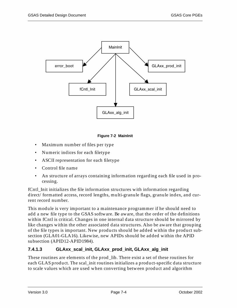
GSAS Detailed Design Document GSAS Core PGEs
• Maximum number of files per type
• Numeric indices for each filetype
• ASCII representation for each filetype
• Control file name
• An structure of arrays containing information regarding each file used in pro-cessing.
fCntl_Init initializes the file information structures with information regarding direct/formatted access, record lengths, multi-granule flags, granule index, and cur-rent record number.
This module is very important to a maintenance programmer if he should need to add a new file type to the GSAS software. Be aware, that the order of the definitions within fCntl is critical. Changes in one internal data structure should be mirrored by like changes within the other associated data structures. Also be aware that grouping of the file types is important. New products should be added within the product sub-section (GLA01-GLA16). Likewise, new APIDs should be added within the APID subsection (APID12-APID1984).
7.4.1.3 GLAxx_scal_init, GLAxx_prod_init, GLAxx_alg_init
These routines are elements of the prod_lib. There exist a set of these routines for each GLAS product. The scal_init routines initializes a product-specific data structure to scale values which are used when converting between product and algorithm
Figure 7-2 MainInit
MainInit
GLAxx_scal_init
error_boot
fCntl_Init
GLAxx_alg_init
GLAxx_prod_init
Version 3.0 Page 7-4 October 2002

GSAS Core PGEs GSAS Detailed Design Document
units. The prod_init and alg_init routines initializes the respective product and algo-rithm data structures to initial and/or invalid values.
7.4.2 eCntl_Init
eCntl_Init is a routine within eCntl_mod, which is local to each PGE. eCntl_mod con-tains the local execution flags which the Manager uses to control process flow. eCntl_Init initializes these flags. These flags are later set by GetControl based on val-ues within the control file.
7.4.3 GetControl
GetControl is a routine local to each specific PGE. This routine reads and parses the control file. It’s structure chart is in Figure 7-3. GetControl performs the following functions:
• Initializes standard control structures (init_StdCntl)
• Opens the control file. (OpenCF)
• Reads the control file until it finds the specified section header.
• Reads the section contents, parsing local and standard (parse_StdCntl) control file entries.
• Sets control flags based on control file entries.
• Closes the control file at the end of the section.
• Performs sanity-checking.
Of particular importance in the routine is the fact that it parses control entries which are specific to each individual PGE. Execution and option flags are defined in a local eCntl module. GetControl sets these flags based on parsed control values. If a mainte-nance programmer needs to add another control flag to a PGE, he must make changes in both eCntl_mod and GetControl.
Figure 7-3 GetControl
GetControl
init_StdCntl
OpenCF Parse_StdCntl
Sanity_Check
October 2002 Page 7-5 Version 3.0

GSAS Detailed Design Document GSAS Core PGEs
7.4.3.1 Init_StdCntl
Init_StdCntl is a subroutine within the StdCntl_mod of the exec_lib. It initializes the text representation of standard (i.e.: common to all PGEs) control file elements.
7.4.3.2 OpenCF
OpenCF is a subroutine within the StdCntl_mod of the exec_lib. It uses a system call to get the value of the control file argument. Platform-specific defines are used here to set the correct position of the argument within the argument list. After getting the name of the control file, OpenCF opens the specified file and scans the file for the start of the specified section. If the control file cannot be opened, a fatal error is returned to the calling process.
7.4.3.3 Parse_StdCntl
Parse_StdCntl is a subroutine within the StdCntl_mod of the exec_lib. It takes control file entries common to all PGEs and parses them, filling the appropriate data struc-ture. In the case of INPUT_FILE and OUTPUT_FILE controls, the routine will attempt to decode the filetype from the filename and fill the appropriate file control structure.
7.4.3.4 Sanity_Check
Sanity_Check is a subroutine within the local GetControl module. It will examine the parsed execution flags and file control structures in order to determine if the control file specifications are valid for the specific PGE. Each PGE has a set of pre-determined rules which dictate what combination of flags and files are appropriate for the defined execution scenarios. Errors will be generated if Sanity_Check finds a problem with the control file configuration.
7.4.4 OpenFiles
OpenFiles is an element of the exec_lib. It opens the first granule of each filetype specified in the control file. The files are opened as direct or formatted based on infor-mation in the file control structure. Normally, OpenFiles assigns a unit to each file it opens and reassigns that same unit to each subsequent granule of that particular file-type. However, in the case of multi-file granules (indicated by a flag in the file control structure), OpenFiles will assign unique units to each file of the first granule and open all files of the first granule. Those files which are not opened are checked for existence and readability.
7.4.5 PrintCntl
PrintCntl is a subroutine of the StdCntl module within the exec_lib. It writes the con-trol file contents to the ANC06 log file.
7.4.6 Write_LibVer
Write_LibVer is an element of the exec_lib. It writes foundation library version infor-mation to the ANC06 log file.
Version 3.0 Page 7-6 October 2002

GSAS Core PGEs GSAS Detailed Design Document
7.4.7 ReadAnc
ReadAnc is an element of the exec_lib. It calls subroutines within the anc_lib to read all requested static ancillary files. The contents of these files are kept in core memory, and, by definition, only read once per execution.
Some special cases exist within ReadAnc:
• If available, the first two ANC01 header files are read via ReadAnc, but subse-quent ANC01 header files are read in a time-synchronized fashion within ReadData. Subsystem-specific MET routines read the actual MET science data.
• Precision Orbit Determination files (ANC08) are not read, but the number of POD files available are counted and this count is stored in a global variable within anc08_pod_mod for later use. A POD data structure is initialized based on the number of files available.
• Precision Attitude files (ANC09) are via a special routine which converts the provided GPS time to UTC time. A flag is set which can be used to determine if valid PAD data exist.
• ANC29 and ANC32 files are read into memory and sorted to account for potential PDS boundary problems. The ANC29.32 design is documented in more detail in the GLAS_L0proc and GLAS_L1A sections.
7.4.8 Write_AncVer
Write_AncVer is an element of the exec_lib. It writes any version information regard-ing ancillary files which were read to the ANC06 log file.
7.4.9 ReadData
ReadData is an element of the exec_lib. It calls subroutines to read one second of requested dynamic ancillary and product data in a time-synchronized fashion. It also seemlessly handles end-of-granule conditions and sets file-specific data availability flags in the appropriate file control structure. Figure 7-4 shows the structure chart for ReadData.
Data are read in a logical order which allows lower-numbered products to pass val-ues forward to data structures of higher-level products. See Section 6.5 for more information regarding the “pass-thru” concept and product/algorithm data conver-sion.
The time-synchronization methodology used by ReadData is rather complex. The fol-lowing algorithm will attempt to describe the procedure:
• Save time and index of last data read.
• Initialize global time and index to invalid
• Loop through each input file type we are to synchronize
- Set data time and index to invalid
- Get the current granule index of the current filetype
October 2002 Page 7-7 Version 3.0

GSAS Detailed Design Document GSAS Core PGEs
- Set the readnew flag to false.
- Loop within the current granule of the current filetype unless the file is not available or we reach EOF
- Read a data record (ReadRecord)
- Cycle if EOF
- Cycle if data time < specified start time
- Set sync time to data time of record we just read
- Exit Interior Loop
- We exit exterior loop when we have a sync time and data time >= sync time +- limit. If we exceeded the limit, decrement the counter and fill the record with invalids. Write error message regarding data gap.
Figure 7-4 ReadData
ReadData
ReadRecord InvalidRecord read_met_hdr
ReadGLA00
ReadGLAxx
GLAxx_P2A
Pass_GLAxx
ReadANC09
next_granule
GLAxx_prod_init
GLAxx_alg_init
read_gla00_index read_apid19 read_apid25
read_apid35
read_apid55
Version 3.0 Page 7-8 October 2002

GSAS Core PGEs GSAS Detailed Design Document
• Check all input files from which we sync for EOF. If all EOF, then set end-of-processing flag and return to calling routine.
• If requested, synchronize ANC09 with data time.
• If requested, synchronize ANC01 with data time. Since we keep 2 ANC01 header files in memory, move the 2nd to the 1st and read a new one into the 1st until data are synchronized.
Note that custom read subroutines are required for APIDs 19, 25, 35 and 55. These are required since these APIDs have data misalignments while prevent them from being read in the standard way.
7.4.9.1 ReadRecord
ReadRecord is an internal subroutine to ReadData. It calls file-specific routines to read one second of the requested data type. ReadRecord will seemlessly move across multiple granules, if necessary. If unsuccessful in reading the requested record, it will set the specific data structure to invalid values and return a flag indicating failure.
7.4.9.2 next_granule
next_granule is an internal subroutine to ReadData. It closes the current granule and open the next, if available. File control structures are set to indicate success or failure.
7.4.9.3 InvalidRec
InvalidRec is an internal subroutine to ReadData. It calls file-specific routines to set the data structures of the target file to invalid values.
7.4.10 Managers
Managers are routines local to each specific PGE. Managers control and execute pro-cess-specific tasks. The use of a Manager routine in a PGE is entirely optional. The purpose of a manager is to provide a software layer between the fairly generic main routine and the task-specific subroutines or subsystem libraries. A good rule of thumb is to use a Manager for complex processing jobs, but to simply insert code into the main routine for relatively simple tasks.
7.4.11 MainWrap
MainWrap is an element of the exec_lib. This routine is called just before the end of execution to close any open files and write summary data to ANC06. This summary data includes:
• The number of each type of status message encountered.
• The number of each type of error message encountered.
• The number of records read for each input file used.
• The number of records written for each output file created.
October 2002 Page 7-9 Version 3.0

GSAS Detailed Design Document GSAS Core PGEs
Version 3.0 Page 7-10 October 2002

Section 8
GLAS_L0proc
8.1 Overview
GLAS Level 0 APID files will normally be distributed as a PDS (Production Data Set) in approximately 6 hour segments or as an EDS (Expedited Data Set) which will be distributed as a Pass Data Dump. There will be several files, each containing a spe-cific APID record for the segment. These segments will be sets of real-time and play-back data received from the polar ground stations. The software that will pre-process GLAS L0 data is the GLAS Level-0 Processor (GLAS_L0proc).
8.2 Function
GLAS_L0proc is a utility PGE that will time synchronize GLA00 APIDs in a manner such that records within different GLAS products may be easily correlated. To do this GLAS_L0proc creates a unique number (rec_ndx) for each packet of data collected by the GLAS instrument. This index will be assigned to the matching records within each Level 0 APID and will account for the 0.25 second waveform Altimeter Digitizer packets
GLAS_L0proc will read each input APID and ancillary file listed in the control file and produce a single index file (ANC29) and a single GPS time correction file (ANC32). The ANC29 file will contain an index to each record in the set of files in the PDS/EDS. The program will group the data in one-second intervals. The ANC32 file will be used during L1A processing to assist in precise laser shot time-tagging.
GLAS_L0proc will also perform limited error checking on the APIDs it reads. It will signal an error if more than the maximum allowed APID records fall within a second and write a warning message to ANC06. Several fields within the APID primary header will be checked against reference values. These errors will be flagged and recorded. Duplicate APID records are checked, flagged and recorded, as well.
The core GLAS PGEs are used as a model for GLAS_L0proc. A major difference in the GLAS_L0proc implementation is that it reads the APIDs one file at a time, rather than synchronously reading all the APIDs record by record. Despite this difference, a great deal of the PGE model was used to create GLAS_L0proc, which will ease software maintenance chores.
Developer experience is that working with L0 spacecraft data can entail a great deal of debugging with regards to both software and the actual data. With this in mind, a significant amount of debug code is embedded within GLAS_L0proc. This code can be turned on with compiler flags but will generate an extensive amount of output. This output is very useful for debugging purposes but can drastically slow execution time. The recommended method of running with debugging turned on is to redirect stdout to a file which can be examined after the run.
October 2002 Page 8-1 Version 3.0

GSAS Detailed Design Document GLAS_L0proc
GLAS_L0proc records statistics such as the number of missing records, number of received records, number of bad records, etc. The software checks for too many occurrences of an APID per second. Duplicate data is flagged as an error (warning not fatal) and the message written to ANC06. Quality issues are tracked and reports made of any problems/potential problems.
8.3 Approach
• GLAS_L0proc uses many of the standard routines from the model GSAS PGE with only minor changes.
• GLAS_L0proc does not perform partial/selective processing or reprocessing. There are no execution flags defined within GLAS_L0proc. Start and stop time are required on control file INPUT_FILE and OUTPUT_FILE specifications for consistency, but are not used.
• GLAS_L0proc uses the operating system-based qsort for sorting tasks. Glue code written in C is used in conjunction with qsort.
• Several constants are needed by GLAS_L0proc processing. Constants include such things at mission elapsed time (MET) offsets, APID identification code, APID record lengths, and sort order keys. These constants are included within the GLA00 product module in order to facilitate code reuse and ease configu-ration management.
• The manager functionality is within the main GLAS_L0proc routine.
• ReadData is not used since data is read file-by-file, rather than record-by-record.
8.4 Input and Output Files
Table 8-1 lists the required inputs to GLAS_L0proc. Table 8-2 lists the outputs created by GLAS_L0proc. Files which are specific to GLAS_L0proc are documented in this section. See the appropriate section of this document or the GLAS Science Data Man-agement Plan for details regarding the those files not specific to GLAS_L0proc.
Table 8-1 GLAS_L0proc Inputs
File Spec Type Source Short Description
gla00*_??.dat Level-0 APID EDOS GLAS Level-0 APID files (one file per each APID type).
anc07*_00.dat Static Ancillary Science Team GLAS error file.
anc07*_01.dat Static Ancillary Science Team GLAS global constants file.
anc33*.dat Dynamic Ancillary ISIPS Operations Counter-to-UTC conversion file.
Control File Control ISIPS Operations Control file.
Version 3.0 Page 8-2 October 2002

GLAS_L0proc GSAS Detailed Design Document
8.4.1 GLA00 APID Files
The GLA00 APIDs are Level-0 multi-rate spacecraft data files provided to the GLAS data processing facility by EDOS. There is a separate file for each specific APID type received from the spacecraft. These files are fully documented by the GLAS Instru-ment Team and within the GLAS L1A ATBD. These APIDs are listed in Table 8-3.
Table 8-2 GLAS_L0proc Outputs
File Spec Type Destination Short Description
anc29*.dat Dynamic Ancillary GLAS_L1A Index file correlating APID times.
anc32*.dat Dynamic Ancillary GLAS_L1A GPS time correction file used for precision timing of GLAS data.
anc06*.dat Dynamic Ancillary ISIPS Operations Standard metadata/processing log file.
Table 8-3 Supported APIDs
APID Description
12 Altimeter Digitizer Large Sci Pkt
13 Altimeter Digitizer Small Sci Pkt
14 Altimeter Digitizer Eng Pkt
15 Photon Counter Sci Pkt
16 Photon Counter Eng Pkt
17 Cloud Digitizer Sci Pkt
18 Cloud Digitizer Eng Pkt
19 Ancillary Science Pkt
20 CT HW telemetry #1 Data Pkt
21 CT HW Telemetry #2 Data Pkt
22 CT HW Telemetry #3 Data Pkt
23 CT HW telemetry #4 Data Pkt
24 Small Software #1 Tlm
25 Large Software Telemetry #1 Packet
26 LPA Data Pkt
27 Memory Dwell Packets 1
28 Memory Dwell Packets 2
31 DSP Code Memory Dump
October 2002 Page 8-3 Version 3.0

GSAS Detailed Design Document GLAS_L0proc
8.4.2 ANC33 MET Counter to UTC Conversion File
The ANC33 file is used to convert mission-elapsed time (MET), which is provided in the APIDs, to GLAS-standard UTC time. Since the MET can be re-set by a roll-over or a spacecraft upset it is important that this file be maintained and provided to the GLAS processing facility in a timely manner. The file is delivered to ISIPS from the ISF as described in the ISF/ISIPS Interface Control Document.
ANC33 file is a ANSI text file. Each line contains data for a single entry in the file (data should not be hard wrapped). Comment lines are allowed and prepended by a # character. Each line contains the following information:
d_shdr_count <sp> d_shdr_count_prap <sp> d_utc <sp> d_glas_osc_rate <sp> d_sc_osc_rate <sp> d_tdelay_digtzr <sp> d_rdelay_digtzr <sp> d_plTbias <sp> d_plRbias <sp> i_trkr_subject1 <sp> i_trkr_subject2 <sp> i_trkr_subject2 <sp>implement_time
Each field is defined in Table 8-4.
32 DSP Data Memory Dump
33 C & T Dwell Packet
34 Event Message Packet
35 Memory Dump Packet
36 Table Dump Packet
38 Boresite Calibration Packet
48 GLAS Data Types Packet
49 Command History Packet
50 CT HW telemetry #5 Data Pkt
55 Large Software Telemetry #2 Packet
126 LPA Test Packet
1984 GLAS PRAP Packet
Table 8-4 ANC33 Field Descriptions
Field Description
d_shdr_count double precision: the counter value in the secondary header on MOST APIDS
d_shdr_count_prap doube precision: the counter value in the secondary header of PRAP
Table 8-3 Supported APIDs (Continued)
APID Description
Version 3.0 Page 8-4 October 2002

GLAS_L0proc GSAS Detailed Design Document
Note that the Implement_time is the UTC time at which this conversion was valid. GLAS_L0proc uses the designated start time of the first APID specified in the control file to find the correct position within the ANC33 file based on the Implement_time field.
8.4.3 Control File
The control file format and common elements are documented in Section 5 of this document. Elements specific to GLAS_L0proc are described here.
The control file section delimiter for GLAS_L0proc is:
=GLAS_L0P
Since GLAS_L0proc has no requirement for execution scenarios, there are no unique keywords for the GLAS_L0proc control file. GLAS_L0proc will perform all functions based on the presence of input and output files within the control file.
8.4.4 ANC29 Index File
The ANC29 index file provides GLAS_L1A with a method of time-correlating the GLAS APID files. It contains an index record for every record in the input APID files. ANC29 is a binary, fixed-length record file. Its format and fields are described in Table 8-5.
8.4.5 ANC32 GPS File
The ANC32 GPS file provides GLAS_L1A with a method of computing precise tim-ing calculations based on the last update of the onboard GPS. It contains records
d_utc double precison: the J2000 UTC time in seconds to which the counter val-ues are converted
d_glas_osc_rate double precision: the GLAS oscillator rate
d_sc_osc_rate double precision: the Spacecraft oscillator rate
d_tdelay_digtzr double precision: time delay for digitizer in seconds
d_rdelay_digtzr double precision: internal range delay for digitizer in m
d_plTbias double precision: post launch time bias in seconds
d_plRbias double precision: post launch range bias in m
i_trkr_subject(1) integer: the subject indicator for LRS tracker 0
i_trkr_subject(2) integer: the subject indicator for LRS tracker 1
i_trkr_subject(3) integer: the subject indicator for LRS tracker 2
d_implement_time double precision: the J2000 UTC time in seconds where the data are first valid
Table 8-4 ANC33 Field Descriptions (Continued)
Field Description
October 2002 Page 8-5 Version 3.0

GSAS Detailed Design Document GLAS_L0proc
which identify each time the GPS clock is updated within the APID packets. ANC33 is a binary, fixed-length record file. Its format is described in Table 8-6.
Table 8-5 ANC29 Format/Description
Variable Type Bytes Description
utctime double precision 8 J2000 UTC time in seconds. Computed from the MET counter in each APID’s secondary header.
rec_ndx long integer 4 Mission-unique index number assigned to the set of APIDs defined by a one second duration and group-ing rules. This number will be assigned to corre-sponding data records in every GLAS data product. The value is nominally (utctime - launchtime) * 10, in seconds.
shot_ctr long integer 4 The appropriate shot counter from each APID.
rec_num long integer 4 The physical record number of the corresponding data within the APID file.
apid long integer 4 The APID number (assigned by the spacecraft team) of the APID.
DQFlag long integer 4 Data quality flag.
sort_order short integer 2 Sort order (for internal use).
spare short integer 24 Spare bytes to align data structure to 8-byte bound-ary.
Table 8-6 ANC32 Format/Description
Variable Type Bytes Description
rec_ndx long integer 4 Mission-unique index number assigned to the set of APIDs defined by a one second duration and grouping rules. This number will be assigned to corresponding data records in every GLAS data product. The value is nominally (utctime - launchtime) * 10, in seconds.
i_ScPosPktShot short integer 2 Shot counter within APID 19 position packet, starting at byte location1182.
i_useflag short integer 2 Flag indicating if the data are valid (0=valid, other=not valid).
utctime double precision 8 UTC time in J2000 seconds where GPS update occurred. This value corresponds exactly to a UTC time in the ANC29 file.
FTLatch double precision 8 Frequency board latch counter within APID19, starting at byte location 1195.
Version 3.0 Page 8-6 October 2002

GLAS_L0proc GSAS Detailed Design Document
8.5 Design
Figure 8-1 shows the top-level structure chart of GLAS_L0proc. The basic processing algorithm is summarized below:
• Initialize (MainInit)
• Set the local execution flags (eCntrl_Init)
• Parse the Control File (GetControl)
• Open the specified files (OpenFiles)
• Print the control file (Print_Cntl)
• Read static ancillary files (ReadAnc)
• Write version info (Write_LibVer, Write_AncVer)
• Until all APID files are read...
- Read APIDs and fill index and gps arrays (readglop)
• Sort the index array (sort_gla00_index)
• Sort the GPS array (sort_gps)
• Convert the MET time into UTC time (utc_time_conversion)
• Group the APID records and assign rec_ndx (IndexGrouping)
• Check the index array for duplicates
• Write the index arrays to file
• Assign rec_ndx to GPS array entries
• Validate data within GPS array and set useflag appropriately
• Write GPS array to file
• Close all files and generate summaries (MainWrap)
ScPosPktGMET double precision 8 MET counts within APID 19 position packet, starting at byte location 1184.
d_VTCW double precision 8 BCTCW latch value within APID19 starting at byte location 1142.
d_VTCWp double precision 8 VTCW value at time of 0.1Hz pulse within APID19 starting at byte location 1182.
GPSTime double precision 8 GPS receiver time in counts within APID19 starting at byte location 1172.
GPSppsGMET double precision 8 MET for GPS 0.1hz counter within APID19 starting at byte location 1201.
Table 8-6 ANC32 Format/Description (Continued)
Variable Type Bytes Description
October 2002 Page 8-7 Version 3.0

GSAS Detailed Design Document GLAS_L0proc
8.5.1 PGE Core Routines
Except where noted, the following PGE core routines are used exactly as defined in the Core PGE Section of this document.
• MainInit
• eCntrl_Init
• GetControl
• OpenFiles
• Print_Cntl
• Write_LibVer
• ReadANC
• Write_AncVer
• MainWrap
Exceptions to normal core routine conventions include:
• eCntl_Init does not define or set execution flags.
• GetControl does not parse any execution flags.
• Start and stop times are required on the INPUT/OUTPUT_FILE assignments, but are not used by GLAS_L0proc to delimit processing. However, the start time of the first APID specified is used as a reference time when finding the correct coefficient for MET-to-UTC conversion. It is critical that this time is specified correctly.
Figure 8-1 GLAS_L0proc Structure Chart
GLAS_L0proc
PGE Core Routines
MainIniteCntrl_InitGetControlOpenFilesPrint_Cntl
Write_LibVerReadANC
Write_AncVer
ReadGLOP
sort_gla00_index sort_gps
IndexGrouping
MainWrap
utc_time_conversion
Version 3.0 Page 8-8 October 2002

GLAS_L0proc GSAS Detailed Design Document
8.5.2 ReadGLOP
ReadGLOP is a subroutine within the local glop_mod module. The glop_mod itself contains several important constants. Since GLAS_L0proc creates its index and GPS arrays in memory, a maximum length for each array is defined in this module. The arrays themselves are defined and allocated in this module, as well.
ReadGLOP is called by the main GLAS_L0proc routine once for each APID which is to be processed. ReadGLOP uses the APID number to read each record of the APID into the appropriate data structure.
ReadGLOP uses standard Fortran direct-to-structure reads to read most APIDs. However, several APIDs are not aligned on 4-byte boundaries. For these, ReadGLOP calls specialized read subroutines which exist within the GLA00_mod module of the product library.
If the APID read is an Ancillary Science Packet (APID19), GPS time is compared with the previous GPS time. If a change has occurred, a GPS array element is filled with the appropriate data.
The primary header of each APID record is converted and checked for error condi-tions. Error checking includes the following:
• Primary header version = 0
• Primary header APID number = expected APID
• Primary header APID size = expected_APID_size – (header_size – 1) (actual value of the offset is 7)
• Primary header secondary header flag /= 0
• Primary header sequence count delta = 1
Duplicate records are checked by comparing the sequence counter and utctime against previous values.
Fields within the index structure are filled and a “sort rank” is assigned based on the APID type. This “sort rank” is temporarily assigned to the spare 4 bytes at the end of the data structure. The shot counter is converted from a signed to unsigned value before assignment.
Since the MET-to-UTC conversion has not yet been performed, the MET counter is assigned to the utctime. However, an APID-specific offset is added to the MET counter for alignment purposes in order to account for processing delays aboard the spacecraft. These values were provided by the instrument developers and are defined in the GLA00_mod module within the product library.
8.5.3 sort_gla00_index
Sort_gla00_index is a C routine local to GLAS_L0proc. It provides a comparison func-tion for the system qsort routine and calls qsort with the index array. qsort returns an index array sorted by utctime (primary) and sort rank (secondary). Sorting the index provides a list of interspersed APID records in time/rank order. Sorting is necessary
October 2002 Page 8-9 Version 3.0

GSAS Detailed Design Document GLAS_L0proc
so that the index_grouping module can correctly assign a rec_ndx to the correct group of corresponding APID records.
An important programmer note is that a C header file (gla00_index.h) is required for sort_gla00_index. If a programmer changes the Index file data structure, they must change the gla00_index.h file in a corresponding manner.
8.5.4 sort_gps
Sort_gps is a C routine local to GLAS_L0proc which is nearly identical to sort_gla00_index. It sorts the GPS array by utctime using a comparison routine with the system qsort call. (This is actually done more for safety than necessity.)
The same caveat applies here as does with sort_gla00_index. A C header file (gps_index.h) is required for sort_gps. If a programmer changes the GPS file data structure, they must change the gps_index.h file in a corresponding manner.
8.5.5 utc_time_conversion
UTC_time_conversion is a routine local to GLAS_L0proc. It reads reference values from ANC33 and uses those values to convert MET counter values within the index array to UTC time.
The routine is passed the start time (taken from the control file entry) of the lowest-numbered APID which has been read. It uses this as it’s initial time and searches through the ANC33 file for the first implement time greater than or equal to the ini-tial time.
Once it has found the correct implement time, it loops through the index array and uses the associated refMET_Counts, refUTC_seconds, and Interval to convert the MET counter to UTC time within the index. While looping, it checks to see if the pre-viously computed UTC time is greater than the next implement time. If so, it reads the associated ANC33 values and uses those for the next UTC conversions.
Additionally, while looping through the index file, the routine checks the GPS array for matches between the APID19 index MET counter and GPS MET counter. If a match is found, the GPS MET counter is converted to UTC time.
The UTC time conversion calculation is performed as follows:
UTC time = refUTC_seconds + (MET counter - refMET_Counts) * Interval
8.5.6 Index_Grouping
Index_grouping is a routine local to GLAS_L0proc. It scans through the index array and assigns rec_ndx values based on a data alignment algorithm.
Sort_gla00_index has already sorted the index array based on MET counts and sort rank. Based on information from the instrument team, certain APIDs are guaranteed to have the same MET counter value for a particular second of data. The sort rank takes this into account and sorts these APIDs at a higher level than others. Addition-ally, the sort order also accounts for importance, guaranteeing that if an APID record
Version 3.0 Page 8-10 October 2002

GLAS_L0proc GSAS Detailed Design Document
exists for a certain second, it will be in a fixed position relative to other APIDs within the one second interval.
The routine loops through the index array. When it detects one of the higher-ranked APIDs, it computes a rec_ndx from the UTC time. This rec_ndx is assigned to the cur-rent APID record and subsequent APID records until another higher-ranked APID is detected. During the period of assigning the rec_ndx, several error checks are per-formed. These are:
• The number of specific APID types assigned the same rec_ndx is checked against a reference maximum-APID-per-second reference (which is defined in GLA00_mod.) If the maximum of a specific APID is exceeded, the rec_ndx value is recomputed and assigned to the current and subsequent APIDs.
• The shot counter values of specific APIDs (AD_LgSci, AD_SmSci, AD_Eng, PC_Sci, PC_Eng, CD_Sci, CD_Eng, AN_Sci, LPA) are checked for consistency. If the shot counters within the same rec_ndx are inconsistent, the rec_ndx value is recomputed and assigned to the current and subsequent APIDs
October 2002 Page 8-11 Version 3.0

GSAS Detailed Design Document GLAS_L0proc
Version 3.0 Page 8-12 October 2002

Section 9
GLAS_L1A
9.1 Overview
GLAS_L1A is a core GSAS PGE. It uses the L1A subsystem to create GLAS Level 1A data from the Level 0 GLAS instrument data products. GLAS_L1A will use the ANC29 and ANC32 files created by GLAS_L0proc to time-synchronously read the appropriate GLA00 APID files.
9.2 Function
The L1A process includes applying calibration equations determined during GLAS system testing to convert the measured counts into engineering units. The conver-sions of the counts to engineering units will be one or more of several types: straight polynomial conversion based on the measurement counts; multi-variable conver-sions with dependence on additional measurements such as temperature; special conversions based on a complex dependence of several measurements, interpretation of data, table look-up, and geophysical based conversions. Some data will not require conversion and will be retained in counts. The Stellar Reference System (SRS) atti-tude and position data and the GPS data will be from standard existing systems sim-ilar to those used on other spacecraft. The conversions and calibration equations for the L1A subsystem are defined the L1A ATBD.
The altimeter data, including the waveforms, are packaged into the GLA01 data product. The atmospheric data from the photon counters and the cloud digitizer, as well as supporting data, are packaged into the GLA02 data product. Both GLA01 and GLA02 include location data obtained from the predicted orbit file. The GLAS instru-ment engineering and housekeeping data are stored in the GLA03 data product. The SRS and GPS data along with the laser pointing monitor data will be packaged into the GLA04 data product.
9.3 Design Approach
The following design criteria are specific to GLAS_L1A.
• GLAS_L1A fully uses the standard routines from the model GSAS PGE.
• GLAS_L1A can perform partial processing, but not reprocessing. GLAS_L1A does perform time-based selective processing. There are, however, dependen-cies between L1A_Atm and L1A_Alt. Partial-processing will not yield the same results for certain parameters as full-processing.
• The ANC29 file (created by GLAS_L0proc) is used to read GLA00 data from the appropriate APID file in the correct order.
October 2002 Page 9-1 Version 3.0

GSAS Detailed Design Document GLAS_L1A
• Due to issues due to aligning multi-rate data across PDS boundaries, the ANC29 and ANC32 files are read into core and re-sorted. This is a break from the concept of normal record-by-record processing.
• L1AMgr is specific to the L1A subsystem. The L1A manager is used to control all L1A-specific science algorithm processes and interfaces directly with the L1A subsystem.
9.4 Input and Output Files
Table 9-1 lists the required inputs to GLAS_L1A. Table 9-2 lists the outputs created by GLAS_L1A. See the GLAS Data Products Specifications Volumes or GLAS Science Data Management Plan for details regarding the these files.
9.5 GLAS_L1A PGE
Figure 9-1 shows the top-level structure chart of GLAS_L1A. The basic processing algorithm is summarized below:
• Initialize (MainInit)
• Set the local execution flags (eCntrl_Init)
• Parse the Control File (GetControl)
Table 9-1 GLAS_L1A Inputs
File Spec Type Source Short Description
gla00*_??.dat Level-0 APID EDOS Level-0 APID files (one file per each APID type).
anc07*_00.dat Static Ancillary Science Team Error file.
anc07*_01.dat Static Ancillary Science Team Global constants file.
anc07*_05.dat Static Ancillary Science Team L1A constants file.
anc25*.dat Dynamic Ancillary Science Team GPS/UTC conversion file.
anc29*.dat Dynamic Ancillary GLAS_L0proc APID index file.
anc32*.dat Dynamic Ancillary GLAS_L0proc GPS time correlation file.
anc33*.dat Dynamic Ancillary Science Team UTC time conversion file.
anc20*.dat Dynamic Ancillary UTexas Predicted orbit file.
anc45*_01.dat Static Ancillary Science Team GLA01 metadata input file.
anc45*_02.dat Static Ancillary Science Team GLA02 metadata input file.
anc45*_03.dat Static Ancillary Science Team GLA03 metadata input file.
anc45*_04.dat Static Ancillary Science Team GLA04 metadata input file.
Control File Control ISIPS Operations Control file.
Version 3.0 Page 9-2 October 2002

GLAS_L1A GSAS Detailed Design Document
• Open the specified files (OpenFiles)
• Print the control file (Print_Cntl)
• Read ancillary files (ReadAnc)
• Write version info (Write_LibVer, Write_AncVer)
• Until all data are processed...
- Execute the L1A_Manager
• Close all files and generate summaries (MainWrap)
Table 9-2 GLAS_L1A Outputs
File Spec Type Destination Short Description
gla01*.dat L1A Product GLAS_L1A GLAS L1A Altimetry product file. Contains the waveforms and the altimeter and timing data required to produce higher level range and elevation products.
gla02*.dat L1A Product GLAS_Atm GLAS L1A Atmosphere product file. Contains the normalized backscatter, photon counter, cloud digitizer, timing, andlocation data required to pro-duce the higher level atmo-sphere data products.
gla03*.dat L1A Product Archive L1A Engineering product file. Contains the GLAS instrument’s engineering and housekeeping data.
gla04*_01.dat L1A Products UTEXAS L1A LPA product file.
gla04*_02.dat L1A Products UTEXAS L1A LRS product file.
gla04*_03.dat L1A Products UTEXAS L1A GYRO product file.
gla04*_04.dat L1A Products UTEXAS L1A IST product file.
gla04*_05.dat L1A Products UTEXAS L1A BST product file.
gla04*_06.dat L1A Products UTEXAS L1A SCPA product file.
qap01*.dat L1A Quality QA L1A Altimetry quality file.
qap02*.dat L1A Quality QA L1A Atmosphere quality file.
qap03*.dat L1A Quality QA L1A Engineering quality file.
qap04*.dat L1A Quality QA L1A SRS/GPS/laser pointing quality files.
anc06*.dat Dynamic Ancillary ISIPS Operations Standard metadata/processing log file.
October 2002 Page 9-3 Version 3.0

GSAS Detailed Design Document GLAS_L1A
9.5.1 PGE Core Routines
PGE core routines are used exactly as defined in the Core PGE Section of this docu-ment.
• MainInit
• eCntrl_Init
• GetControl
• OpenFiles
• Print_Cntl
• Write_LibVer
• ReadANC
• Write_AncVer
• ReadData
• MainWrap
9.6 L1A Manager (L1A_Mgr)
The L1A Manager controls execution of the L1A subsystem, passes variables from the GLA00 APIDs to the L1A products, and handles granule start/stop. The manager controls execution of the science algorithms based on flags received from the control file via GLAS_L1A. Figure 9-2 shows the L1A Manager Structure Chart. Figure 9-3 shows a flow chart of the L1A Manager.
L1A_Mgr is passed arrays of output file control structures and execution flags. It accesses product and algorithm data directly from the requisite public data struc-
Figure 9-1 GLAS_L1A Structure Chart
GLAS_L1APGE Core Routines
MainIniteCntrl_InitGetControlOpenFilesPrint_Cntl
Write_LibVerReadANC
Write_AncVerWrite_eCtrlReadData
L1A_Mgrcheckoutput(PGE core)
MainWrap
Version 3.0 Page 9-4 October 2002

GLAS_L1A GSAS Detailed Design Document
tures. Execution flags are defined in eCntl_mod; file control structures defined in the fCntl_mod component of the exec_lib, and product/algorithm data within the GLA00, GLA01, GLA02, GLA03, and GLA04 components of the product_lib.
The first thing the manager does is check for an end-of-granule condition within each defined output file by comparing the nominal time of data (set by ReadData_mod) with the appropriate stop time within the specific file data structure. If an end-of-granule condition is detected, final QA routines are called and the product and QA files are closed. If another granule of the same type has been specified in the control file, the manager opens the appropriate product and QA files and loops to verify the stop time of the new granule is greater than the nominal time of data.
After checking the granule times, processing begins. The manager calls calc_shot_time, which computes precise 40 per second timing information. It then calls C_CalcSpLoc which computes 40 spot locations based on the 40 per second tim-ing information and the location of satellite position interpolated from the predicted orbit file (ANC20).
Next, the manager executes several science algorithms based on its execution flags and data availability. L_Eng, L_Alt, L_Atm, and L_Att are called. Each returns a flag indicating if the appropriate data product should be written. Values which are passed directly from one product to another are set appropriately.
QA routines are called to process QA information and the WriteL1A routine is called with the appropriate flags to write data to the product files. Before writing a record, WriteL1A verifies that the appropriate output file exists and that the nominal time of data is greater than the start time specified in file control structure. If the nominal
Figure 9-2 L1A_Mgr Structure Chart
L1A_Mgr
L_ALT
PGE Core Routines
glaxx_hdr_initglaxx_hdr_updatecom_hdr_updateWrite_glaxx_hdr
GLAS_Error
L_ALT_QA
L_ATM
L_ATM_QA
L_ENG
L_ENG_QA
L_ATT
L_ATT_QA
calc_shot_time
est_shot_time
C_InterpPOD
October 2002 Page 9-5 Version 3.0

GSAS Detailed Design Document GLAS_L1A
time is less than the start time, the data record is not written. An appropriate error message is written to ANC06 if a record is skipped.
9.7 PGE/Manager Implementation Details
This section discusses specific aspects of the PGE/Manager implementation which should be addressed in more detail.
9.7.1 ANC29/ANC32/GLA00 Input
ANC29 data are handled differently than most core PGE I/O. Due to potential PDS boundary problems (for example, the waveform data for a particular second may be on a different PDS than the corresponding ancillary science data), all input ANC29 granules are read into memory by the ReadAnc core PGE routine. This array is dynamically allocated based on the number of records indicated in each ANC29 file header. The internal file number from which the ANC29 data are read is stored into a spare byte in the array so that when GLA00 data are read, the corresponding GLA00
Figure 9-3 L1A Manager Flow Chart
L_Eng
calc_shot_time
c_calc_sploc
perform_L_alt AND ALT
data_avail?
L_ALT
perform_L_Atm AND ATM data_avail?
L_Atm
perform_L_eng
Wrapup
c_intrpPOD
Set d_thresh_xing, GLA02 rec_ndx, time, location
L1A_Mgr7 / 2 1 / 0 0
Set GLA01 rec_ndx,shot time, location
call GLAS_Error
N
N
Y
Y
Y
N
Version 3.0 Page 9-6 October 2002

GLAS_L1A GSAS Detailed Design Document
file is used. After the ANC29 granules are read into memory, the data are sorted to guarantee the correct time order. ANC32 data are loaded into memory similarly.
ReadData actually “reads” the ANC29 and ANC32 data on a second-by-second basis from memory. As the specialized ANC29/32 I/O was a fairly late design decision, this implementation minimized changes to the ReadData logic. ReadData uses the ANC29 data to read the correct records from the various GLA00 APID files. It reads 1-second groups of APID records using the physical record number, APID type, and internal file number to determine the correct position within the GLA00 files.
ReadData determines the content of a 1-second group by examining ANC29 rec_ndx values. “rec_ndx” is described fully in the GLAS_L0proc section, but suffice to say, it is an integer corresponding to 0.1 second utctimes. For the most part, rec_ndx values for APIDs of a particular second are the same exact value. However, in the case of APIDs which straddle PGEs, the values may not be exactly the same. To handle this case, ReadData will consider that rec_ndx values which correspond within 0.9 sec-onds are part of the same second. This value is a constant defined in GLA00_mod.f90 as “rec_ndx_slop”.
9.7.2 Missing APIDs
Different GLAS APID packets originate from different subsystems of the GLAS instrument. Depending upon the instrument state, APIDs may or may not be present in the data stream. In addition, data drop-outs present the possibility of missing data.
The L1A Manager sets an array of flags (APID_Av_Flg) to indicate present or missing data. A signal flag is set for each 1-second APID record. The complication arises when checking the 1/4 second APID waveform records AD_LgSci, AD_SmSci). In order to figure out which of the four records are missing, the manager examines shot counters. By definition, the shot counter in the Ancillary Science (AN_Sci) APID will match the first shot counter in the first corresponding waveform record. The manager uses this knowledge to set positional flags that indicate which of the 1/4 waveform APIDs are missing.
If at least one of the waveform records or the AN_Sci record is available, L1A_Mgr calls L_Alt and a GLA01 record is written. If the Photon Counter Science (PC_Sci), Cloud Digitizer Science (CD_Sci), or AN_Sci records are available, L1A_Mgr calls L_Atm and a GLA02 record is written.
The GLA01 product file is a little different than the other GLAS products in that it contains different record types. It has the following record types: main, large wave-form, and small waveform. The main record type occurs once per second. The large waveform type occurs five per second. The small waveform type occurs twice per second. A record identifier (i_gla01_rectype) within each record identifies what type that record is. If at least one of the waveform records or the AN_Sci record is avail-able, the Main record type exists in GLA01 for a particular second. If at least one of the waveform records is available, the waveform type (small or large) records exist in GLA01 for that second.
October 2002 Page 9-7 Version 3.0
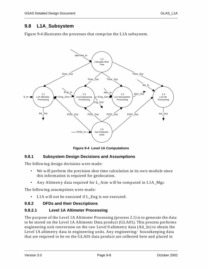
GSAS Detailed Design Document GLAS_L1A
9.8 L1A_Subsystem
Figure 9-4 illustrates the processes that comprise the L1A subsystem.
9.8.1 Subsystem Design Decisions and Assumptions
The following design decisions were made:
• We will perform the precision shot time calculation in its own module since this information is required for geolocation.
• Any Altimetry data required for L_Atm will be computed in L1A_Mgr.
The following assumptions were made:
• L1A will not be executed if L_Eng is not executed.
9.8.2 DFDs and their Descriptions
9.8.2.1 Level 1A Altimeter Processing
The purpose of the Level 1A Altimeter Processing (process 2.1) is to generate the data to be stored on the Level 1A Altimeter Data product (GLA01). This process performs engineering unit conversion on the raw Level 0 altimetry data (Alt_In) to obtain the Level 1A altimetry data in engineering units. Any engineering/ housekeeping data that are required to be on the GLA01 data product are collected here and placed in
Figure 9-4 Level 1A Computations
2.2L1A Atmosphere
Processing
2.1L1A Altimetry Processing
2.3L1A Engineering
Processing
2.4L1A Att
Processing
2.5Calculate Shot
Time
2.6Get Predicted
Orbit
lt_In
Eng_In Atm_In
rawTime_In
POD_In
Att_In
Time_Out
Time_Out Time_Out
Time_Out
Eng_Out Eng_Out
POD_Out POD_Out POD_Out POD_Out
Atm_Out
Eng_Out
Alt_Out Att_Out
Version 3.0 Page 9-8 October 2002

GLAS_L1A GSAS Detailed Design Document
the output structure. Quality assessment computations are performed, collected and placed in an output QA structure.
9.8.2.2 L1A Atmosphere Processing
The purpose of the L1A Atmosphere Processing (process 2.2) is to generate the data to be stored on the Level 1A Atmosphere Data product (GLA02). This process per-forms engineering unit conversion on the raw Level 0 atmosphere data (Atm_In) to obtain the Level 1A atmosphere data in engineering units. Any engineering/ house-keeping data that are required to be on the GLA02 data product are collected here and placed in the output structure. Quality assessment computations are performed, collected and placed in an output QA structure.
9.8.2.3 Engineering Data Processing
The purpose of the Engineering Data Processing (process 2.3) is to generate the data for the Level 1A Engineering Data product (GLA03). This process performs engineer-ing unit conversion on the raw Level 0 engineering/housekeeping data (Eng_In) to obtain the Level 1A engineering data in engineering units. Any Level 0 data that are not stored on either GLA01, GLA02, or GLA04 are collected here and placed in the output structure. Quality assessment computations are performed, collected and placed in an output QA structure.
Additionally, specific parameters of the Eng_Out structure are passed to the Altime-try and Atmosphere processors.
9.8.2.4 Collect Instrument and S/C Position and Attitude
The purpose of process 2.4 is to collect the GPS data, instrument and S/C position and attitude data and to generate the L1A Position and Attitude data product (GLA04). The APIDs used to generate GLA04 include APID19, APID26, and APID1984. The GLA04 product is required for input to the precision orbit and atti-tude determination algorithms. This process checks the Level 0 packets for errors, configures the data for output and collects QA data.
Due to internal spacecraft/instrument timing issues all data corresponding to one second of GLA04 data may not be within one second of APID1984. To align the LRS and IST data to corresponding APID19 shot times, a 6 second double-buffering algo-rithm is used to match the LRS and IST data with corresponding APID19 shots. To complicate matters, the LRS and IST data occur at a rate of 10/second, whereas the APID19 shots occur at a rate of 40/second. The algorithm finds the APID19 shots closest to the LRS/IST data and merges the APID19 and APID1984 data into a single one second GLA04 record.
9.8.2.5 Calculate Shot Time
The Calculate Shot Time process (process 2.5) will generate the precise time of each laser shot. The actual methodology of the time calculation depends upon the pres-ence of the Ancillary Science (AN_Sci) APID. If AN_Sci is not present, 40-per-second time is generated linearly using a 0.025 increment. If AN_Sci is available, the time will be calculated from the laser fire time, GPS time, and the GPS latch time. Offsets
October 2002 Page 9-9 Version 3.0

GSAS Detailed Design Document GLAS_L1A
and calibration factors will be applied as necessary. The process is fully described in the L1A ATBD.
9.8.2.6 Get Predicted Location
The Get Predicted Location process (process 2.6) obtains the latitude and longitude for each shot from the predicted orbit file using common routines. The shot times are input, the predicted orbit file is interpolated to get the spacecraft position vector for each shot time, and then the latitude and longitude are computed from the position vector. The common routines c_intrpPOD and c_calc_sploc will be used for the calcu-lations. The common routines will be called directly by the L1A Manager; it is not necessary to generate code for the Level 1A Computations subsystem.
Version 3.0 Page 9-10 October 2002

Section 10
GLAS_Alt
GLAS_Alt is a core GSAS PGE. It uses the Waveform and Elevation subsystems to create GLAS Level 1B and 2 data from the Level 1 GLAS altimetry data products. GLAS_Alt will read the GLA01 file created by GLAS_L1A to create the GLA05, GLA06, and GLA12-15 products. GLAS_Alt can also read the GLA05 file which it cre-ated in a separate processing scenario to create GLA06 and GLA12-15. Additionally, GLAS_Alt can read the GLA05 and GLA06 files created in a separate processing sce-nario to generate GLA12-15.
10.1 Function
GLAS_Alt comprises both the Waveform and Elevation subsystems.
The Level 1B Waveforms subsystem computes the geolocation, and produces wave-form-based information required to produce the elevation products (GLA05).
The Levels 1B and 2 Elevation Computation subsystem generates all elevation Stan-dard Data Products, associated Processing Quality Assessment data, and related computations. The Level 1B subsystem creates parameters for a Level 1B time-ordered global product (GLA06) with a geodetically corrected surface elevation using the same standard algorithm used for ice sheet regions. The Level 2 subsystem deter-mines region specific (ice sheet, sea ice, land, and ocean regions) elevation parame-ters for Level 2 time-ordered regional products (GLA12, GLA13, GLA14, and GLA15).
10.2 Design Approach
The following design criteria are specific to GLAS_Alt
• GLAS_Alt fully uses the standard routines from the model GSAS PGE.
• GLAS_Alt can perform partial processing. However, since the Elevations sub-system needs data from GLA05, it is not possible to create GLA12-15 with only GLA06 as an input.
• All products are output at one record per 1 sec. However, GLA12-15 are only written when the footprint location falls within the respective regional mask.
• ANC01 meteorological data sets are required at times before and after the time of the input product data.
10.3 Input and Output Files
Table 10-1 lists the required inputs to GLAS_Alt. Table 10-2 lists the outputs created by GLAS_Alt. See the GLAS Data Products Specifications Volumes or GLAS Science
October 2002 Page 10-1 Version 3.0

GSAS Detailed Design Document GLAS_Alt
Data Management Plan for details regarding the these files. Those files which are only required by specific subsystems are noted within the table..
Table 10-1 GLAS_Alt Inputs
File Spec Type Source Short Description
anc01*.dat Dynamic Ancillary met_util Meteorological subset files. Data sets at times before and after the time of the profile are interpolated to the time of the profile.
anc04*.dat Dynamic Ancillary UTexas IERS Polar Motion and Earth Rotation Data File.
anc07*_0000.dat Static Ancillary Science Team Error file.
anc07*_0001.dat Static Ancillary Science Team Global constants file.
anc07*_0003.dat Static Ancillary Science Team Waveform constants file.*Waveform only
anc07*_0004.dat Static Ancillary Science Team Elevations constant file.*Elevation only
anc08*.dat Dynamic Ancillary UTexas Precision Orbit file.
anc09*.dat Dynamic Ancillary UTexas Precision Attitude file.
anc12*_0000.dat Static Ancillary Science Team Coarse DEM file*Elevation only.
anc12*_0001.dat Static Ancillary Science Team Fine DEM file*Elevation only.
anc13*.dat Static Ancillary Science Team Geoid file*Elevation only.
anc16*.dat Static Ancillary Science Team Load tide coefficients file*Elevation only.
anc17*.dat Static Ancillary Science Team Ocean tide coefficients file*Elevation only.
anc25*.dat Dynamic Ancillary Science Team GPS/UTC conversion file.
anc27*_0000.dat Static Ancillary Science Team Coarse regional mask file.
anc27*_0001.dat Static Ancillary Science Team Fine regional mask file.
anc33*.dat Dynamic Ancillary Science Team UTC time conversion file.
anc45*_0001.dat Static Ancillary Science Team GLA01 metadata input file.*Waveform only
anc45*_0005.dat Static Ancillary Science Team GLA05 metadata input file.
anc45*_0006.dat Static Ancillary Science Team GLA06 metadata input file.
Version 3.0 Page 10-2 October 2002

GLAS_Alt GSAS Detailed Design Document
anc45*_0012.dat Static Ancillary Science Team GLA12 metadata input file.
anc45*_0013.dat Static Ancillary Science Team GLA13 metadata input file.
anc45*_0014.dat Static Ancillary Science Team GLA14 metadata input file.
anc45*_0015.dat Static Ancillary Science Team GLA15 metadata input file.
Control File Control ISIPS Operations Control file.
gla01*_.dat Level-1A Product GLAS_L1A L1A Altimetry product file.*Waveform only.
gla05*_.dat Level-1B Product GLAS_Alt L1B Waveform product file.*Elevation only
gla06*_.dat Level-1B Product GLAS_Alt L1A Elevation product file.*Elevation only
Table 10-2 GLAS_Alt Outputs
File Spec Type Destination Short Description
gla05*.dat L1B Alt Product Archive/GLAS_Alt The level 1B waveform parame-terization product file. Contains the output from the waveform characterization procedure and other parameters required to calculate surface slope and relief characteristics.
gla06*.dat L2 Alt Product Archive/GLAS_Alt L1B elevation data product file. Contains the surface elevation, surface roughness assuming no slope, surface slope assuming no roughness and geodetic and atmospheric corrections for the range.
gla12*.dat L2 Alt Product Archive L2 ice sheet altimetry product file. Contains the ice sheet ele-vation and elevation distribution calculated from algorithms fine-tuned for ice sheet returns.
gla13*.dat L2 Alt Product Archive L2 sea ice altimetry product file. Contains the sea ice freeboard and sea ice roughness calcu-lated from algorithms fine-tuned for sea ice returns.
Table 10-1 GLAS_Alt Inputs (Continued)
File Spec Type Source Short Description
October 2002 Page 10-3 Version 3.0

GSAS Detailed Design Document GLAS_Alt
10.4 GLAS_Alt
Figure 10-1 shows the top-level structure chart of GLAS_Alt. The basic processing algorithm is summarized below:
• Initialize (MainInit)
• Set the local execution flags (eCntrl_Init)
• Parse the Control File (GetControl)
• Open the specified files (OpenFiles)
• Print the control file (Print_Cntl)
• Read ancillary files (ReadAnc)
• Write version info (Write_LibVer, Write_AncVer)
• Until all data are processed...
- Execute the WF_Manager, based on Control
- Execute the Elev_Manager, based on Control
• Close all files and generate summaries (MainWrap)
gla14*.dat L2 Alt Product Archive L2 land altimetry product file. Contains the land elevation and land elevation distribution calcu-lated from algorithms fine-tuned for land returns.
gla15*.dat L2 Alt Product Archive L2 ocean altimetry product file. Contains ocean elevation and small-scale roughness calcu-lated from algorithms fine-tuned for ocean returns.
qap05*.dat L1B Alt Quality QA L1B waveform parameterization quality file.
qap06*.dat L2 Alt Quality QA L2 elevation data quality file.
qap12*.dat L2 Alt Quality QA L2 ice sheet altimetry quality file.
qap13*.dat L2 Alt Quality QA L2 sea ice altimetry quality file.
qap14*.dat L2 Alt Quality QA L2 land altimetry quality file.
qap15*.dat L2 Alt Quality QA L2 ocean altimetry quality file.
anc06*.dat Dynamic Ancillary ISIPS Operations Standard metadata/processing log file.
Table 10-2 GLAS_Alt Outputs (Continued)
File Spec Type Destination Short Description
Version 3.0 Page 10-4 October 2002

GLAS_Alt GSAS Detailed Design Document
10.4.1 PGE Core Routines
PGE core routines are used exactly as defined in the Core PGE Section of this docu-ment.
• MainInit
• eCntrl_Init
• GetControl
• OpenFiles
• Print_Cntl
• Write_LibVer
• ReadANC
• Write_AncVer
• ReadData
• MainWrap
10.5 Waveform Manager (WF_Mgr)
The Atm Manager controls execution of the Waveform subsystem, passes variables from the input GLA01 product to the output GLA05 product, and handles granule start/stop. The manager controls execution of the waveform science algorithms based on flags received from GLAS_Alt. The manager is only executed if at least one of its execution flags is set. Figure 10-2 shows the WF_Mgr structure chart.
Figure 10-1 GLAS_Alt Structure Chart
GLAS_AltPGE Core Routines
MainIniteCntrl_InitGetControlOpenFilesPrint_Cntl
Write_LibVerReadANC
Write_AncVerWrite_eCtrlReadData
WF_Mgr
checkoutput(PGE core)
MainWrap
Elev_Mgr
October 2002 Page 10-5 Version 3.0

GSAS Detailed Design Document GLAS_Alt
Figure 10-2 WF_Mgr Structure Chart
WF_Mgr
W_FunctionalFt
PGE Core Routines
glaxx_hdr_initglaxx_hdr_updatecom_hdr_updateWrite_glaxx_hdr
GLAS_Error
Write_WF
W_CompFuFStats
W_InitFFQA
W_CompAssStats
W_InitAQSA
W_Assess
Version 3.0 Page 10-6 October 2002

GLAS_Alt GSAS Detailed Design Document
Figure 10-3 shows a flow chart of WF_Mgr.
Figure 10-3 WF Manager Flowchart
WFMgr
Start of Procedure GLA05_hdr_init
com_hdr_update
GLA05_hdr_update
true
End of Granule WF_Wrapuptrue
GLA05_hdr_update
Write_GLA05_hdr
Time Exceeds QA Interval W_CompAssStats
true
W_InitAsQA
W_Assess
W_FunctionalFt
Write_WF
All Bad Frames Return
Return
true
( l_noLandCalc, l_noOtherCalc )
( l_noLandCalc, l_noOtherCalc, l_noGeo )
( l_noLandCalc, l_noOtherCalc, l_noGeo )
October 2002 Page 10-7 Version 3.0

GSAS Detailed Design Document GLAS_Alt
WF_Mgr is passed arrays of output file control structures and execution flags. It accesses product and algorithm data directly from the requisite public data struc-tures. Execution flags are defined in eCntl_mod; file control structures defined in the fCntl_mod component of the exec_lib, and product/algorithm data within the GLA01 and GLA05 components of the product_lib.
The first thing the manager does is check for an end-of-granule condition within each defined output file by comparing the nominal time of data (set by ReadData_mod) with the appropriate stop time within the specific file data structure. If an end-of-granule condition is detected, wrap-up and final QA routines are called and the product and QA files are closed. If another granule of the same type has been speci-fied in the control file, the manager opens the appropriate product and QA files and loops to verify the stop time of the new granule is greater than the nominal time of data.
After checking the granule times, processing begins. The manager calls common library geolocation and DEM routines to compute position and elevation and tide routines to get tide data.
Next, the manager executes several science algorithms based on its execution flags and data availability. These algorithms are discussed in the DFD section. Each returns a flag indicating if the GLA05 data product should be written. Values which are passed directly from one product to another are set appropriately.
QA routines are called to process QA information and the WriteWF routine is called with the appropriate flags to write data to the product file. Before writing a record, WriteWF verifies that the appropriate output file exists and that the nominal time of data is greater than the start time specified in file control structure. If the nominal time is less than the start time, the data record is not written. An appropriate error message is written to ANC06 if a record is skipped.
10.6 Elevation Manager (Elev_Mgr)
The Elevation Manager controls execution of the Elevation subsystems, passes vari-ables from the input GLA05/06 product to the output GLA06 and GLA12-15 prod-ucts, and handles granule start/stop. The manager controls execution of the elevation science algorithms based on flags received from GLAS_Alt. The manager is only exe-cuted if at least one of its execution flags is set. Figure 10-4 shows the Elev_Mgr struc-ture chart. Figure 10-5 shows a flow chart of Elev_Mgr.Elev_Mgr is passed arrays of output file control structures and execution flags. It accesses product and algorithm data directly from the requisite public data structures. Execution flags are defined in eCntl_mod; file control structures defined in the fCntl_mod component of the exec_lib, and product/algorithm data within the GLA05/06 and GLA12-15 compo-nents of the product_lib.
The first thing the manager does is check for an end-of-granule condition within each defined output file by comparing the nominal time of data (set by ReadData_mod) with the appropriate stop time within the specific file data structure. If an end-of-granule condition is detected, wrap-up and final QA routines are called and the
Version 3.0 Page 10-8 October 2002
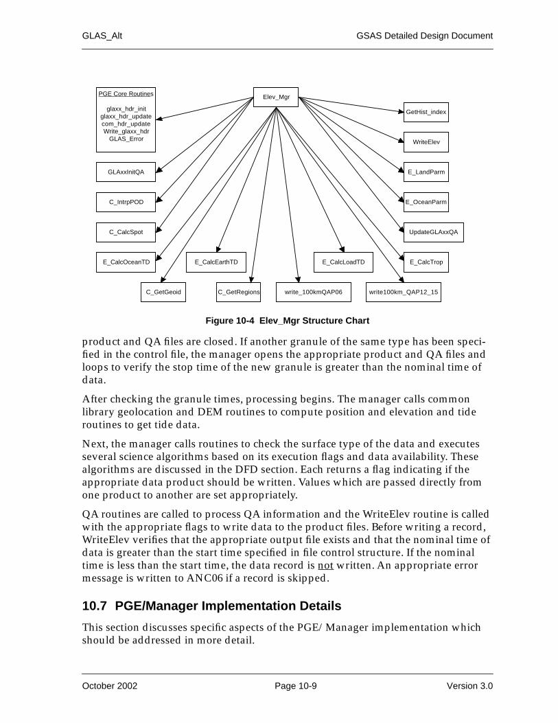
GLAS_Alt GSAS Detailed Design Document
product and QA files are closed. If another granule of the same type has been speci-fied in the control file, the manager opens the appropriate product and QA files and loops to verify the stop time of the new granule is greater than the nominal time of data.
After checking the granule times, processing begins. The manager calls common library geolocation and DEM routines to compute position and elevation and tide routines to get tide data.
Next, the manager calls routines to check the surface type of the data and executes several science algorithms based on its execution flags and data availability. These algorithms are discussed in the DFD section. Each returns a flag indicating if the appropriate data product should be written. Values which are passed directly from one product to another are set appropriately.
QA routines are called to process QA information and the WriteElev routine is called with the appropriate flags to write data to the product files. Before writing a record, WriteElev verifies that the appropriate output file exists and that the nominal time of data is greater than the start time specified in file control structure. If the nominal time is less than the start time, the data record is not written. An appropriate error message is written to ANC06 if a record is skipped.
10.7 PGE/Manager Implementation Details
This section discusses specific aspects of the PGE/Manager implementation which should be addressed in more detail.
Figure 10-4 Elev_Mgr Structure Chart
Elev_Mgr
C_GetGeoid
PGE Core Routines
glaxx_hdr_initglaxx_hdr_updatecom_hdr_updateWrite_glaxx_hdr
GLAS_Error
E_CalcOceanTD E_CalcEarthTD E_CalcLoadTD
GLAxxInitQA
C_IntrpPOD
C_CalcSpot
E_CalcTrop
C_GetRegions write_100kmQAP06 write100km_QAP12_15
UpdateGLAxxQA
E_OceanParm
E_LandParm
WriteElev
GetHist_index
October 2002 Page 10-9 Version 3.0
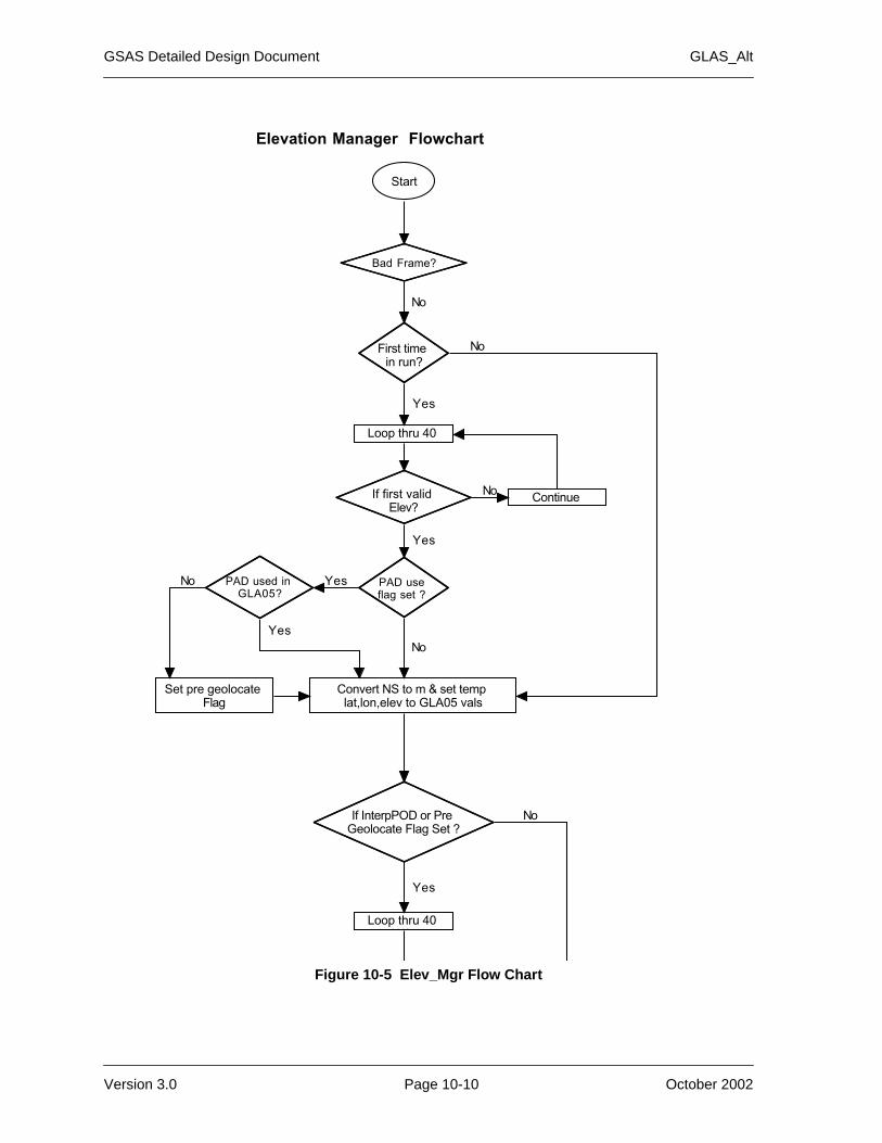
GSAS Detailed Design Document GLAS_Alt
Figure 10-5 Elev_Mgr Flow Chart
Start
Bad Frame?
Elevation Manager Flowchart
PAD used in GLA05?
Convert NS to m & set temp lat,lon,elev to GLA05 vals
PAD use flag set ?
Set pre geolocate Flag
If first valid Elev?
YesNo
First time in run?
Yes
Loop thru 40 Wf
No
Yes
Yes
Continue No
No
No
Loop thru 40 Wf
If InterpPOD or Pre Geolocate Flag Set ?
Yes
No
Version 3.0 Page 10-10 October 2002

GLAS_Alt GSAS Detailed Design Document
Figure 10-5 Elev_Mgr Flow Chart (Continued)
Calc Geoid
Calc Ocean Td
geoid?
Yes
Ocean Td Corr?
Earth Td corr?
Yes
No
Yes
No
No
Geolocate Using Prelim Range, & set to temp lat,lon,elev
InterpPOD?
InterpPOD
Yes
Loop thru 40 Wf
Calc 2/sec parameters
No
Valid Elev?
Yes
No
Loop once for first valid elevation, then for last valid elevation. This is needed to get the 2/sec parameters
October 2002 Page 10-11 Version 3.0

GSAS Detailed Design Document GLAS_Alt
Figure 10-5 Elev_Mgr Flow Chart (Continued)
Calc Load Td
Calc Earth Tide
Met Corr ?
Load Td Corr?
Loop thru 40 WFs
Bad Elev ?
Yes
Yes No
Continue Loop ?
Loop thru 40, WF (intervals of 10)
Valid Elev ?
Loop thru next 9 WF for 1st Valid Elev
If Found ?
No
Yes
Yes
No
Yes
Set Load Tide Invalid
No
Continue Loop ?Yes
No
No
Yes
No
Version 3.0 Page 10-12 October 2002

GLAS_Alt GSAS Detailed Design Document
Figure 10-5 Elev_Mgr Flow Chart (Continued)
Calc Met CorrSet Trop Invalid
Loop thru 40 Wf
Identify Regions
Assign Reg. Sp. Ranges for GLA06
A region is identified as set if any of the 40 shots fall in it.
Set To Invalid:GLA06: Thresh Ret,Sig Beg,Sig End,SigElev,Roughness,Slope, #Pks Smooth wfm,centroid Rng
No All Regions found or end of loop?
Yes
Continue?
No
Yes
Write 100Km QA ?
Loop thru 40 Wf
No
Write 100km QAYes
Interpolate and sum tide & trop corrs
Write 100Km QAP only for reqions requested
Interpolate and sum valid corrections
If Std Wf No Sig ?
Valid IS Range?No Yes
No
Set GLA06 Loc, Elev Invalid
Yes
October 2002 Page 10-13 Version 3.0

GSAS Detailed Design Document GLAS_Alt
Figure 10-5 Elev_Mgr Flow Chart (Continued)
Calc DEM
Calc Spot Loc
DEM ?
Yes
Set Spot Loc= GLA05 lat,lon. Elev=invalid
No
Valid WF Fit?Slope/ Roughness?
No
Calc Slope/Rough
Update GLA06QA
Yes
No
Ice Sheet?
Yes
Valid IS Range?
No Yes
Yes
No
Valid Lat/Lon?
Yes
No
Slope/ Roughness?
Set Slope/Rough = invalid
Yes
Set DEM invalid
DEM ?
Set Slope/ Rough invalid
Slope/Rough ?
Yes
No
Set GLA12 Loc, Elev Invalid
Ice Sheet?
Yes
No
Yes
No
No
Version 3.0 Page 10-14 October 2002

GLAS_Alt GSAS Detailed Design Document
Figure 10-5 Elev_Mgr Flow Chart (Continued)
Calc DEM
Valid WF Fit?
Slope/ Roughness?
Yes
GLA12 Slope,Rough=GLA06slope,rough
No
Update GLA12QA
Yes
Sea Ice?
Yes
No
No
em Invalid
Set DEM invalid
Yes
Set Slope/ Rough invalid
Slope/Rough ?
No
Sea Ice?
Yes
No
Yes
No
October 2002 Page 10-15 Version 3.0

GSAS Detailed Design Document GLAS_Alt
Figure 10-5 Elev_Mgr Flow Chart (Continued)
Set To Invalid:GLA13: Thresh Ret, Rng(Ist peak),Avg Elev,Sig Beg,Sig End, Skewness,Std. Dev Last Pk,Chi Sq, Roughness,Num Pks Fit,Centroid Rng
Calc Spot Loc
Valid SI Range?
Set Spot Loc= GLA05 lat,lon. Elev=invalid
No Yes
Valid WF Fit?
Slope/ Roughness?
Yes
Update GLA13QA
Yes
Calc Avg Elev
Valid centroid Range?
Set Avg Elev Invalid
No Yes
Calc DEM
DEM ?
Yes
No
Valid Lat/Lon?
YesSet Dem Invalid
No
Set GLA13 Loc, Elev Invalid
Set DEM invalid
DEM ?
Yes
Set Slope/ Rough invalid
Slope/Rough ?
Yes
No
No
No
No
Version 3.0 Page 10-16 October 2002

GLAS_Alt GSAS Detailed Design Document
Figure 10-5 Elev_Mgr Flow Chart (Continued)
Set To Invalid:GLA15: Thresh Ret,Rng(1st peak),Sig Beg,Sig End, Skewness,Std. Dev Last Pk,Chi Sq, Roughness, Num Pks Fit,centroid Rng
GLA13 Rough=GLA06 rough
Ocean?
Calc Spot Loc
Valid Oc Range?
Set Spot Loc= GLA05 lat,lon. Elev=invalid
No Yes
Yes
Calc Avg Rng Offset
Valid centroid Range?
Set Avg Rng Offset Invalid
No Yes
No
Calc DEM
DEM ?
Yes
Valid Lat/Lon?
Yes
Set Dem Invalid
Set GLA15 Loc, Elev Invalid
Set DEM invalid
DEM ?
Yes
Set Ocean Parms Invalid
Ocean?
Yes
No
No
No
No
Calc High, Low Elev
October 2002 Page 10-17 Version 3.0

GSAS Detailed Design Document GLAS_Alt
Figure 10-5 Elev_Mgr Flow Chart (Continued)
Set To Invalid:GLA14: Thresh Ret,Rng(All peaks),Sig Beg,Sig End,sigma Gaus, amp Gaus,area Gaus,Kurtosis,Skewness,Std. Dev Last Pk,Chi Sq, Slope,Roughness, Num Pks Fit,centroid of peaks
Valid WF Fit?
Update GLA15QA
Yes
Land?
If Alt WF No SIg?
Yes
Valid Land Rng?
Set Spot Loc= GLA05 lat,lon. Elev=invalid
No
Calc Spot Loc
No
Valid WF Fit?
Calc DEM
DEM ?
Yes
No
Valid Lat/Lon?
Yes
Set Dem Invalid
No
Yes
Yes
No
Set GLA14 Loc, Elev Invalid
Set DEM invalid
DEM ?
Yes
No
Yes
Set Land Parms Invalid
No
No
Version 3.0 Page 10-18 October 2002

GLAS_Alt GSAS Detailed Design Document
Figure 10-5 Elev_Mgr Flow Chart (Continued)
End
Write Output
Continue Loop 40 ?
No
Update GLA14QA
Slope/ Roughness?
Yes
Calc Slope/Roughness
Calc Land Parms
No
Yes
Set Slope/ Rough invalid
Slope/Rough ?
Yes
No
October 2002 Page 10-19 Version 3.0

GSAS Detailed Design Document GLAS_Alt
10.7.1 GLA05 Requirement
The original concept of GLAS_Alt was to enable the Elev_Mgr to create GLA12-15 directly from GLA06. However, due to data dependencies, GLA05 input is required (as well as GLA06) when creating GLA12-15.
10.8 WF_Subsystem
The Level 1B Waveforms subsystem computes the geolocation, and produces wave-form-based information required to produce the elevation products (GLA05_SCF)
10.8.1 DFDs and their Descriptions
The Level 1B Waveforms subsystem is divided into two main processes (W_Assess, and W_FunctionalFt) which generate waveform-based information required to pro-duce the elevation products (GLA05). A control flag (w_ctrl) is passed to processes W_Assess and W_FunctionalFt indicating whether processing will be land algorithm only, other-than-land algorithm only, or both, and whether the subprocess W_DetGeo will be called. In addition to producing waveform-based information, processes W_Assess and W_FunctionalFt generate QA data for inclusion in the summary infor-mation product. The following is a description of each of the processes.
10.8.1.1 Assess Waveforms (W_Assess)
.Utilizes the transmitted waveforms (r_wf_trans), received waveforms (r_wf_rec), compression ratios (i_compression), index of compression change (i_ndxCompChg), the PAD pointing vector (d_PADpntgVect), the number of gates in each waveform (i_numGinWF, normally 200 or 544), the number of waveforms in a frame (i_numWFinFrame, normally 40), the filter used by the spacecraft (d_filterOb), the UTC time of the first waveform (d_UTC1stPTime), the time increment from d_UTC1stPTime to each of the 39 other waveforms in the frame (d_dShotTime), the digitizer time of gate 1 of the transmitted pulse (d_TimeGate1Tr), the digitizer time of the last gate of the received waveform (d_TimeGateLRec), background noise (d_bgNoise), the standard deviation of the background noise level calculated by the on board algorithm (d_sDevNsOb - snoise_ob in ATBD), and an array of flags (l_WFqual - indicates if any of the waveforms are invalid) to perform a general assessment of the waveforms including: a check for waveform saturation (i_satFlag, d_pcntSat); defining the noise and the begin and end of signal (d_bg_Noise, d_sDevNoise, i_ndxBegin, d_minRngOff, i_ndxEnd, d_maxRngOff); characterizing the transmitted pulse (d_maxTrAmp, d_areaTr, d_centroidTr, d_parmTr, d_skewTr); computing smoothed waveforms (d_wf_sm, d_maxSmAmp); calculating various shape characteristics for the received waveform (d_maxRecAmp, d_skew, d_kurt, d_centroid); calculating the reference range (d_refRng), and range offsets (d_preRngOff, d_thRtkRngOff); and determining the preliminary latitude, longitude and elevation (d_latPreUncor, d_longPreUncor, d_elevPreUncor).
d_relTime is the relative time of each gate taking account of the compression infor-mation. For example, if the original gates were one nanoseconds apart, and there was
Version 3.0 Page 10-20 October 2002

GLAS_Alt GSAS Detailed Design Document
a compression ratio of 2, then the time of gate 1 (r_wf_rec[1]) would be the average of the times of the first two digitizer gates ((0+1)/2 or 0.5).
d_wf_sm is the smoothed waveform, and d_maxSmAmp is the maximum amplitude of the smoothed waveform.
i_sat_flag indicates whether waveform signal saturation is minimal (normal wave-form processing is applied), moderate (some information on elevation can be approx-imated) or excessive (no waveform processing is applied).
d_pcntSat is the percent saturation for each waveform.
d_bg_Noise is either the observed noise (d_bgNoiseOb), or the calculated back-ground noise, and d_sDevNoise is either the observed noise standard deviation
Figure 10-6 W_Assess
October 2002 Page 10-21 Version 3.0

GSAS Detailed Design Document GLAS_Alt
(d_sDevNsOb), or the standard deviation of the calculated noise. The calculation is performed if anc07%i_nsCal is set, or if the observed noise is zero or invalid and the waveform is not invalid.
d_refRng is the reference range in nanoseconds (the time from the centroid of the transmitted pulse to the time of last gate of the received waveform).
d_maxRngOff is the offset to be added to d_refRng to give the time of the last thresh-old crossing (farthest from the spacecraft).
d_minRngOff is the offset to be added to d_refRng to give the time of the first thresh-old crossing (closest to the spacecraft).
d_preRngOff is the offset to be added to d_refRng to give the time of the preliminary uncorrected range (threshold farthest from spacecraft).
d_thRtkRngOff is the offset to be added to d_refRng to give the time of the retracker threshold.
i_ndxBegin and i_ndxEnd are the indices of the beginning and end of signal of the received waveform.
d_areaRecWF is the area under the received waveform, above the noise, from signal begin through signal end.
d_maxRecAmp is the maximum amplitude of the received waveform.
d_skew is the skewness of the received waveform from signal begin through signal end.
d_kurt is the kurtosis of the received waveform from signal begin through signal end.
d_centroid is the centroid of the received waveform from signal begin through signal end.
d_maxTrAmp is the maximum amplitude of the transmitted pulse.
d_areaTr is the area under the transmitted pulse (all 32 gates).
d_centroidTr is the centroid of the transmitted pulse (all 32 gates).
d_parmTr is the gaussian amplitude, peak location relative to gate one of the trans-mitted pulse, and gaussian sigma of the single peak gaussian fit to the transmitted pulse.
d_skewTr is the skewness of the transmitted pulse.
d_latPreUncor, d_longPreUncor, and d_elevPreUncor are the preliminary, uncor-rected latitude, longitude, and elevation.
l_land, l_ocean, l_icesheet, and l_seaice are flags taken from the region mask indicat-ing the possible presence of land, ocean, icesheet and/or seaice for each waveform.
l_offNadirFlag indicates if the spacecraft is pointed off nadir.
l_PODflag indicates the status of the orbit information.
Version 3.0 Page 10-22 October 2002

GLAS_Alt GSAS Detailed Design Document
l_WFqual is an array of 31 flags for each waveform. These flags include: no signal, no leading edge, no trailing edge, no transmitted pulse, land, ocean, icesheet, seaice, no fit, noise and standard deviation of noise are calculated, maximum iterations during fit, region selected for waveform fit, and invalid waveform.
d_PODposVect is the precision orbit position vector.
l_badFrame indicates if the entire frame is bad.
i_errSeverity indicates the maximum severity of any error occurring during the exe-cution of W_Assess.
October 2002 Page 10-23 Version 3.0
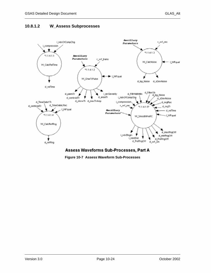
GSAS Detailed Design Document GLAS_Alt
10.8.1.2 W_Assess Subprocesses
Figure 10-7 Assess Waveform Sub-Processes
Version 3.0 Page 10-24 October 2002

GLAS_Alt GSAS Detailed Design Document
Figure 10-7 Assess Waveform Sub-Processes (Continued)
October 2002 Page 10-25 Version 3.0

GSAS Detailed Design Document GLAS_Alt
10.8.1.3 Calculate the WF Functional Fit (W_FunctionalFt)
.Utilizes the waveform (r_wf_rec), the smoothed waveform (d_wf_sm), time (d_relTime), time array indices for the begin & end of signal (iNdxBegin & iNdxEnd), the background noise (d_bg_Noise), the standard deviation of the background noise (d_sDevNoise), the centroid of the received waveform (d_centroid), and the region type(s) (l_land, l_ocean, l_icesheet, and l_seaice) to fit the waveform to a function and return the calculated waveform function parameters (d_parm), the estimated param-eters (d_estParms), the initial number of peaks found (i_nPeakInit), the number of solution peaks found (i_nPeaks), the ranks of the peaks (i_rank), the solution sigmas (d_solnSigmas), the standard deviation of the fit (d_wfFitSDev), a flag indicating if the fit was unsuccessful - i.e. if the normal matrix turns singular (l_fitNogo), and a flag indicating if the fit ended without meeting the convergence criteria (l_fit_maxiter).
Figure 10-7 Assess Waveform Sub-Processes (Continued)
Version 3.0 Page 10-26 October 2002

GLAS_Alt GSAS Detailed Design Document
Figure 10-8 W_FunctionalFt
October 2002 Page 10-27 Version 3.0

GSAS Detailed Design Document GLAS_Alt
10.8.1.4 W_FunctionalFt Subprocesses
Figure 10-9 W_FunctionalFt Subprocesses
Version 3.0 Page 10-28 October 2002

GLAS_Alt GSAS Detailed Design Document
Figure 10-9 W_FunctionalFt Subprocesses (Continued)
October 2002 Page 10-29 Version 3.0

GSAS Detailed Design Document GLAS_Alt
Figure 10-9 W_FunctionalFt Subprocesses (Continued)
Version 3.0 Page 10-30 October 2002

GLAS_Alt GSAS Detailed Design Document
Figure 10-9 W_FunctionalFt Subprocesses (Continued)
October 2002 Page 10-31 Version 3.0

GSAS Detailed Design Document GLAS_Alt
Figure 10-9 W_FunctionalFt Subprocesses (Continued)
Version 3.0 Page 10-32 October 2002

GLAS_Alt GSAS Detailed Design Document
Figure 10-9 W_FunctionalFt Subprocesses (Continued)
October 2002 Page 10-33 Version 3.0

GSAS Detailed Design Document GLAS_Alt
Figure 10-9 W_FunctionalFt Subprocesses (Continued)
Version 3.0 Page 10-34 October 2002

GLAS_Alt GSAS Detailed Design Document
Figure 10-9 W_FunctionalFt Subprocesses (Continued)
October 2002 Page 10-35 Version 3.0
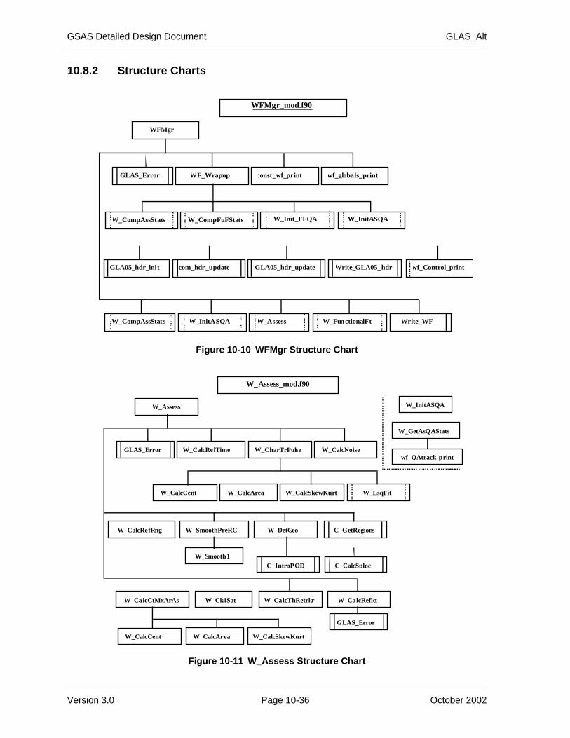
GSAS Detailed Design Document GLAS_Alt
10.8.2 Structure Charts
Figure 10-10 WFMgr Structure Chart
Figure 10-11 W_Assess Structure Chart
WFMgr
const_wf_print wf_globals_printGLAS_Error WF_Wrapup
WFMgr_mod.f90
GLA05_hdr_update Write_GLA05_hdrGLA05_hdr_init com_hdr_update wf_Control_print
W_CompFuFStats W_Init_FFQAW_CompAssStats W_InitASQA
W_Assess W_FunctionalFtW_CompAssStats W_InitASQA Write_WF
W_Assess
W_CharTrPulse W_CalcNoiseGLAS_Error W_CalcRelTime
W_CalcCent W CalcArea W_CalcSkewKurt
W_Assess_mod.f90
W_InitASQA
W_GetAsQAStats
wf_QAtrack_print
W_DetGeo C_GetRegionsW_CalcRefRng
W_CalcThRetrkr W_CalcReflctW_CalcCtMxArAs W_Ck4Sat
W_CalcAreaW_CalcCent W_CalcSkewKurt
GLAS_Error
W_LsqFit
W_SmoothPreRC
W_Smooth1C_IntrpPOD C_CalcSploc
Version 3.0 Page 10-36 October 2002

GLAS_Alt GSAS Detailed Design Document
10.9 Elev_Subsystem
The Levels 1B and 2 Elevation Computation subsystem generates all elevation Stan-dard Data Products, associated Processing Quality Assessment data, and related computations. The Level 1B subsystem creates parameters for a Level 1B time-ordered global product (GLA06_SCF) with a geodetically corrected standard eleva-tion. The Level 2 subsystem determines region specific (ice sheet, sea ice, land, and ocean regions) elevation parameters for Level 2 time-ordered regional products (GLA12_SCF, GLA13_SCF, GLA14_SCF, and GLAS15_SCF).
10.9.1 L1B DFDs and their Descriptions
Below is a breakdown of each of the elevation processes into subprocesses. Each sub-process corresponds to a Fortran 90 subroutine that is called by the elevation man-ager
10.9.1.1 Interpolate POD (C_IntrpPOD)
Utilizes the POD file (ANC08), and time to interpolate the precision vectors for use in geolocation.
Figure 10-12 W_FunctionalFt Structure Chart
W_FunctionalFt
W_GetHstNdxD W_GetHstNDxIGLAS_Error W_ParamWithFit
W_PerformFitW_EstParams W_RankAllPeaks W_GetHstNDxI
W_EstimatesW_Calc2ndDer
W_Reduce_PeaksW_CombinePeak W_RankPeaks W_CombinePeaks
W_CleanPeaks
W_FunctionalFt_mod.f90
W_LsqFit
GLAS_Error
W_RankPeaks
W_CombinePeaks W_GetHstNDxI
W_GetHstNDxI
W_InitFFQA
W_GetFfQAStats
wf_QA_summary_print
October 2002 Page 10-37 Version 3.0

GSAS Detailed Design Document GLAS_Alt
10.9.1.2 Tide Correction Routines (E_CalcLoadTD, E_CalcOceanTD, E_CalcEarthTD)
The tide correction routines consists of three processes which calculate the elevation corrections due to the effects of the load tide, ocean tide, and earth tide. Each process is triggered by a control flag. Following is a brief description of each of the process:
10.9.1.2.1 Compute Load Tide Correction (E_calcLoadTd)
Utilizes the load tide coefficients file to compute the coefficients for the given spot location. Then calculates the load tide correction using the given time.
10.9.1.2.2 Compute Ocean Tide Correction (E_calcOceanTd)
Utilizes the ocean tide coefficients file to compute the coefficients for the given spot location. Then calculates the ocean tide correction using the given time (time).
10.9.1.2.3 Compute Earth Tide Correction (E_calcEarthTd)
Utilizes the earth tide coefficients file to compute the coefficients for the given spot location. Then calculates the earth tide correction using the given time.
Figure 10-13 Level 1B and 2 Elevation DFD
Version 3.0 Page 10-38 October 2002

GLAS_Alt GSAS Detailed Design Document
10.9.1.3 Interpolate Geoids (C_GetGeoid)
Utilizes the spot location to interpolate for the geoid height at that location. This is a common routine used by several processes.
10.9.1.4 Calculate Troposphere Corrections (E_CalcTrop)
Utilizes the met data files, spot location, and elevation (with respect to the geoid), to interpolate spatially for parameters used in the calculation of the tropospheric correc-tions. These corrections are then temporally interpolated to get the tropospheric cor-rections for the given time.
10.9.1.5 Calculate Std surface Elevation and spot loc (C_ CalcSploc)
Utilizes the results from the previous three processes along with the spacecraft posi-tion in ITRF (Inertial Terrestrial Reference Frame), the laser attitude in ITRF, refer-ence range, and ice sheet range offset to calculate surface independent elevation and spot location.
10.9.1.6 Interpolate DEM (E_CalcDEM)
Utilizes the spot location, the Global DEM file, and the DEM mask file to determine the DEM elevation for the specified spot.
Figure 10-14 Level 1B Elevation Computation DFD
October 2002 Page 10-39 Version 3.0

GSAS Detailed Design Document GLAS_Alt
10.9.1.7 Calculate Quality Flag (E_AtmQF)
Utilizes the cloud optical depth and cloud boundary layer height to ascertain the effect of atmospheric problems that would decrease quality of the elevation product. This quality is returned as a flag.
10.9.1.8 Calculate Slope & Roughness (E_CalcSlope)
Utilizes the sigma of the gaussian waveform, transmitted pulse width, and receiver impulse width to calculate the slope and roughness.
10.9.1.9 Create L1B Quality Statistics (update_GLA06QA)
Combines QA data from the previous six processes to create QA statistics for the Level 1B Elevation Computation subsystem
10.9.2 Create L1B Quality Statistics
Combines QA data from the previous six processes to create QA statistics for the Level 1B Elevation Computation subsystem
10.9.3 L2 DFDs and their Descriptions
Below is a breakdown of each of the elevation processes into subprocesses. Each sub-process corresponds to a Fortran 90 subroutine that is called by the elevation man-ager
Figure 10-15 Tide Corrections Routines DFD
Version 3.0 Page 10-40 October 2002

GLAS_Alt GSAS Detailed Design Document
10.9.3.1 Check Region (C_GetRegions)
Utilizes the region masks file and spot location to determine the valid regions for the spot location.
10.9.3.2 Determine Region Spec Elevation and Spot Location (C_CalcSploc)
Utilizes the region specific range (land, sea ice, icesheet, or ocean), POD position vec-tor, PAD vectors, tide corrections, and tropospheric corrections to calculate the region specific elevation and spot location.
10.9.3.3 Calc Reg Params (E_OceanParm, E_LandParm)
Calculates the region specific parameters that have not already been determined ear-lier by the other routines.
10.9.3.4 Interpolate DEM (E_CalcDEM)
Utilizes the region specific spot locations, the Global DEM file, and the DEM mask file to determine the DEM elevation for the specified spot.
Figure 10-16 Calculate Level2 Elevations DFD
October 2002 Page 10-41 Version 3.0

GSAS Detailed Design Document GLAS_Alt
10.9.3.5 Create L2 Elevations QA (update_GLA12QA, update_GLA13QA, update_GLA14QA, update_GLA15QA)
Combines QA data from the processes 5.2.2, 5.2.3, and 5.2.4 to create QA statistics for the Level 2 Elevation Computation subsystem.
10.9.3.6 Create Elevation QA Statistics (wrapUpQAP06, wrapUpQAP12_15)
Wraps up and writes to file the QA Statistics for the Level 1B and 2 Elevation Compu-tation subsystems. WrapUpQAP06 will handle the Level 1B subsystem, while wrapUPQAP12_15 will handle the Level 2 subsystem.
10.9.4 Structure Charts
Figure 10-17 Elevation Manager
Version 3.0 Page 10-42 October 2002

GLAS_Alt GSAS Detailed Design Document
Figure 10-17 Elevation Manager (Continued)
October 2002 Page 10-43 Version 3.0

GSAS Detailed Design Document GLAS_Alt
Figure 10-17 Elevation Manager (Continued)
Version 3.0 Page 10-44 October 2002
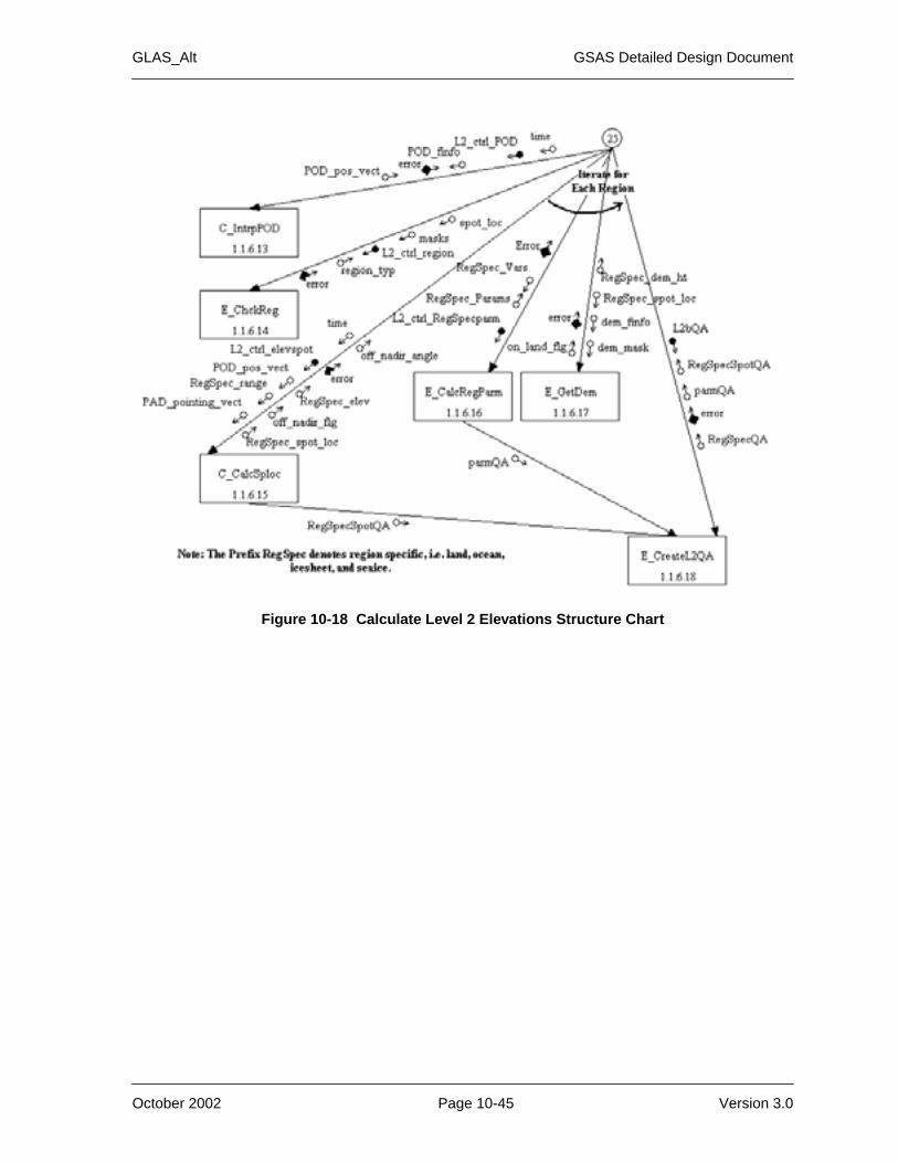
GLAS_Alt GSAS Detailed Design Document
Figure 10-18 Calculate Level 2 Elevations Structure Chart
October 2002 Page 10-45 Version 3.0

GSAS Detailed Design Document GLAS_Alt
Figure 10-19 Tide Correction Routines Structure Chart
Figure 10-20 GetGeoid Structure Chart
Version 3.0 Page 10-46 October 2002

GLAS_Alt GSAS Detailed Design Document
Figure 10-21 Calculate Trop Corrections Structure Chart
October 2002 Page 10-47 Version 3.0

GSAS Detailed Design Document GLAS_Alt
Version 3.0 Page 10-48 October 2002

Section 11
GLAS_Atm
11.1 Overview
GLAS_Atm is a core GSAS PGE. It uses the Atmosphere subsystem to create GLAS Level 1B and 2 data from the Level 1 GLAS atmosphere data products. GLAS_Atm will read the GLA02 file created by GLAS_L1A and the ANC36 file created by Atm_Anc to create the GLA07-11 products.
11.2 Function
The function of the Levels 1B and 2 Atmosphere Computations subsystem is to create atmosphere parameters for the standard data products GLA07-11 and to generate associated metadata and quality assessment (QA) data.
11.3 Design Approach
The following design criteria are specific to GLAS_Atm
• GLAS_Atm fully uses the standard routines from the model GSAS PGE.
• GLAS_Atm can perform partial processing. However, due to the 20 second buffering, the Level 2 data is always processed together even under reprocess-ing scenarios. Data products GLA08-11 are always created together.
• The Level 1B product (GLA07) is output at one record per 1 sec.
• The processing of Level 2 data is buffered for 20 seconds irrespective of time gaps between data records.
• The Level 2 products (GLA08-11) are output at one record per 4 seconds.
• Cloud products are reported at once per 4 seconds, 1 second, and 5 Hz from 21 to 0 km, and at 40 Hz below 4 km.
• Aerosol products are reported at once per 4 seconds from 21 to 0 km and at once per 20 sec from 41 to 21 km.
• Twenty second averaging requires that at least ten seconds of valid profiles are available. Likewise, four second averaging requires that at least two seconds of valid profiles are available.
• Met data sets at times before and after the time of the profile are interpolated to the time of the profile. If either of the met data sets are missing, then the available met data set is used without interpolation. If no met data sets are available, then standard atmosphere data are used instead
October 2002 Page 11-1 Version 3.0

GSAS Detailed Design Document GLAS_Atm
11.4 Input and Output Files
Table 11-1 lists the required inputs to GLAS_Atm. Table 11-2 lists the outputs created by GLAS_Atm. See the GLAS Data Products Specifications Volumes or GLAS Science Data Management Plan for details regarding the these files..
Table 11-1 GLAS_Atm Inputs
File Spec Type Source Short Description
anc01*.dat Dynamic Ancillary met_util Meteorological subset files. Data sets at times before and after the time of the profile are interpolated to the time of the profile. If either of the ANC01 data sets are missing, then the available ANC01 data set is used without interpolation. If no ANC01 data sets are available, then standard atmosphere data are used instead.
anc04*.dat Dynamic Ancillary UTexas IERS Polar Motion and Earth Rotation Data File.
anc07*_0000.dat Static Ancillary Science Team Error file.
anc07*_0001.dat Static Ancillary Science Team Global constants file.
anc07*_0002.dat Static Ancillary Science Team Atm constants file.
anc07*_0005.dat Static Ancillary Science Team L1A constants file.
anc08*.dat Dynamic Ancillary UTexas Precision Orbit file.
anc09*.dat Dynamic Ancillary UTexas Precision Attitude file.
anc12*_0000.dat Static Ancillary Science Team DEM file.
anc12*_0001.dat Static Ancillary Science Team DEM mask file.
anc13*.dat Static Ancillary Science Team Geoid file.
anc18*.dat Static Ancillary Science Team Standard atmosphere file.
anc24*.dat Dynamic Ancillary UTexas Rotation Matrix file.
anc25*.dat Dynamic Ancillary Science Team GPS/UTC conversion file.
anc30*.dat Static Ancillary Science Team Global aerosol categorization map file.
anc31*.dat Static Ancillary Science Team Aerosol tropospheric classifica-tion map file.
anc33*.dat Dynamic Ancillary Science Team UTC time conversion file.
anc35*.dat Static Ancillary Science Team Ozone file.
Version 3.0 Page 11-2 October 2002

GLAS_Atm GSAS Detailed Design Document
anc36*.dat Dynamic Ancillary atm_anc Atmosphere Calibration file.
anc38*.dat Static Ancillary Science Team Multiple-scattering table file.
anc45*_0002.dat Static Ancillary Science Team GLA02 metadata input file.
anc45*_0007.dat Static Ancillary Science Team GLA07 metadata input file.
anc45*_0008.dat Static Ancillary Science Team GLA08 metadata input file.
anc45*_0009.dat Static Ancillary Science Team GLA09 metadata input file.
anc45*_0010.dat Static Ancillary Science Team GLA10 metadata input file.
anc45*_0011.dat Static Ancillary Science Team GLA11 metadata input file.
Control File Control ISIPS Operations Control file.
gla02*_.dat Level-1A Product GLAS_L1A L1A Atmosphere product file.
Table 11-2 GLAS_Atm Outputs
File Spec Type Destination Short Description
gla07*.dat L1B Atm Product Archive L1B Global Backscatter product file. Contains full 532 nm and 1064 nm calibrated attenuated backscatter profiles at 5 times per second, and from 10 to -1 km, at 40 times per second. Also included will be calibration coefficient values and molecular backscatter profiles at once per second.
gla08*.dat L2 Atm Product Archive L2 Planetary Boundary Layer and Elevated Aerosol Layer Height product file. Contains elevated aerosol layer height data consisting of top and bot-tom heights for up to 5 aerosol layers below 20 km at once per 4 seconds, and top and bottom heights for up to 3 aerosol layers above 20 km at once per 20 seconds.
Table 11-1 GLAS_Atm Inputs (Continued)
File Spec Type Source Short Description
October 2002 Page 11-3 Version 3.0

GSAS Detailed Design Document GLAS_Atm
11.5 Functions
Figure 11-1 shows the top-level structure chart of GLAS_Atm. The basic processing algorithm is summarized below:
• Initialize (MainInit)
• Set the local execution flags (eCntrl_Init)
• Parse the Control File (GetControl)
• Open the specified files (OpenFiles)
gla09*.dat L2 Atm Product Archive L2 Cloud Layer Height product file. Contains top and bottom heights for up to 10 layers below 20 km at once per 4 seconds, once per second, 5 times per second, and 40 times per sec-ond (below 4 km only). Ground heights will also be provided at each resolution.
gla10*.dat L2 Atm Product Archive L2 Aerosol Vertical Structure product file. Contains cloud and aerosol backscatter and extinc-tion cross section profiles.
gla11*.dat L2 AtmProduct Archive L2 Thin Cloud/Aerosol product file. Contains optical depths for clouds for up to 10 layers, the planetary boundary layer, and aerosols for up to 8 layers.
qap07*.dat L2 Atm Quality QA L1B Global Backscatter quality file.
qap08*.dat L2 Atm Quality QA L2 Planetary Boundary Layer and Elevated Aerosol Layer Height quality file.
qap09*.dat L2 Atm Quality QA L2 Cloud Layer Height quality file.
qap10*.dat L2 Atm Quality QA L2 Aerosol Vertical Structure quality file.
qap11*.dat L2 Atm Quality QA L2 Thin Cloud/Aerosol quality file.
anc06*.dat Dynamic Ancillary ISIPS Operations Standard metadata/processing log file.
Table 11-2 GLAS_Atm Outputs (Continued)
File Spec Type Destination Short Description
Version 3.0 Page 11-4 October 2002

GLAS_Atm GSAS Detailed Design Document
• Print the control file (Print_Cntl)
• Read ancillary files (ReadAnc)
• Write version info (Write_LibVer, Write_AncVer)
• Until all data are processed...
- Execute the Atm_Manager
• Close all files and generate summaries (MainWrap)
11.5.1 PGE Core Routines
PGE core routines are used exactly as defined in the Core PGE Section of this docu-ment.
• MainInit
• eCntrl_Init
• GetControl
• OpenFiles
• Print_Cntl
• Write_LibVer
• ReadANC
• Write_AncVer
• ReadData
• MainWrap
11.5.2 Atm Manager (Atm_Mgr)
The Atm Manager controls execution of the Atmosphere subsystem, passes variables from the input GLA02 product to the output GLA07-11 products, and handles gran-ule start/stop. The manager controls execution of the science algorithms based on
Figure 11-1 GLAS_Atm Structure Chart
GLAS_AtmPGE Core Routines
MainIniteCntrl_InitGetControlOpenFilesPrint_Cntl
Write_LibVerReadANC
Write_AncVerWrite_eCtrlReadData
Atm_Mgrcheckoutput(PGE core)
MainWrap
October 2002 Page 11-5 Version 3.0

GSAS Detailed Design Document GLAS_Atm
flags received from GLAS_Atm. Figure shows the Atm_Mgr structure chart. Figure
11-3 shows a flow chart of the Atm Manager..
Atm_Mgr is passed arrays of output file control structures and execution flags. It accesses product and algorithm data directly from the requisite public data struc-tures. Execution flags are defined in eCntl_mod; file control structures defined in the fCntl_mod component of the exec_lib, and product/algorithm data within the GLA02 and GLA07-11 components of the product_lib.
The first thing the manager does is check for an end-of-granule condition within each defined output file by comparing the nominal time of data (set by ReadData_mod) with the appropriate stop time within the specific file data structure. If an end-of-granule condition is detected, wrap-up and final QA routines are called and the product and QA files are closed. If another granule of the same type has been speci-fied in the control file, the manager opens the appropriate product and QA files and loops to verify the stop time of the new granule is greater than the nominal time of data.
After checking the granule times, processing begins. The manager calls A_cal_coefs to get calibration coefficients from ANC36. It then calls common library geolocation and DEM routines to compute position and elevation and A_interp_met to get mete-orological data.
Next, the manager buffers the data and executes several science algorithms based on its execution flags and data availability. These algorithms are discussed in the DFD section. Each returns a flag indicating if the appropriate data product should be writ-
Figure 11-2 Atm_Mgr Structure Chart
Atm_Mgr
C_GetGeoid
PGE Core Routines
glaxx_hdr_initglaxx_hdr_updatecom_hdr_updateWrite_glaxx_hdr
GLAS_Error
A_qa_G8_11
C_CalcDEM A_interp_met A_mbscs
A_cal_coefs
C_IntrpPOD
C_CalcSpot
A_rebin_lid
A_bscs A_bscs A_qa_G7 WriteAtm A_buff_data
A_cld_lays
A_pbl_lays
A_aer_lays
A_aer_opt_prop
Version 3.0 Page 11-6 October 2002

GLAS_Atm GSAS Detailed Design Document
Figure 11-3 ATM Manager - Part 1
Call E_GetGeoidto get geoid
Call C_CalcSpLocto get satellite ht
Call C_interp_podto get POD
Call A_met_interpto get MET profs
Call A_mbscsto get molec profs
Call A_rebin_lid to vert align profs
Call A_bscsto get back profs
if (bs_to_end)
AtmMgr
If (start_of_processing) initialize headersLoop through granule times: if current time >= stop time
for GLA07: set end_of_1s_granule flag to 1 Increment to next granule for GLA07
for GLA08-11: set end_of_4s_granule flag to 1
if (bs_only)
True
True
Call A_qa_G7 (end_of_1s_granule flag, end_of_processing flag) to get QA stats for GLA07
if (end_of_1s_granule) average and write QA , then sumif (end_of_processing) average and write QA
else sum
if (bs_only)True
if (end_of_processing)True
if (end_of_1s_granule == 1)
Set end_of_1s_granule flag to 0Increment to next QA granule for GLA07
Call WriteATM (i_write_ctrl) to write GLA07 product
if (.not. no_pod)
if (bs_to_end)
if (bs_to_end)
OR
OR
if (bs_only)
ANDOR
if (end_of_processing)
True
True
Set (i_write_ctrl) = 1 (write GLA07)
Call A_cal_cofsto get calib cofsif (bs_only)
Trueif (bs_to_end)
OR
Call E_CalcDEMto get DEM
Call C_CalcSpLocto get lat/lon/elev
October 2002 Page 11-7 Version 3.0

GSAS Detailed Design Document GLAS_Atm
Figure 11-4 ATM Manager - Part 2
Call A_aer_laysto get aer lays
Call A_aer_opt_propto get optical properties
Call A_cld_laysto get cld hts
Call A_pbl_layto get PBL lay
Call A_buff_data (end_of_4s_granule flag, end_of_processing flag) to buffer 20 secs of data and pass-throughs for 4 sec products
Set i_complete_buf to 0
Return
if (cld_to_end)if (bs_to_end)
Fill 20 sec tmp buffer
Output 20 sec output argumentsClear 20 sec tmp buffers
Reset time t(1)Set i_complete_buf to 1
Call A_qa_G8-11 (end_of_4s_granule flag, end_of_processing flag, i_qa_ctrl)) to get QA stats for GLA08-11
if (end_of_4s_granule or end_of_processing) add to sums, then average and write QAelse add to sums
Call WriteATM (i_write_ctrl) to write GLA08-11 products
if (end_of_4s_granule == 1)
if (time since t(1) <= 20 s)
True
False
Set end_of_4s_granule flag to 0Increment to next granule for GLA08-11
Increment to next QA granule for GLA08-11
if (i_complete_buf == 1)False
if (end_of_processing)
if (end_of_4s_granule == 1)
True
True
Go to to start of bufferingif (end_of_processing)
True
Set (i_write_ctrl) = 2 (write GLA08-11)
False
OR
Version 3.0 Page 11-8 October 2002

GLAS_Atm GSAS Detailed Design Document
ten. Values which are passed directly from one product to another are set appropri-ately.
QA routines are called to process QA information and the WriteAtm routine is called with the appropriate flags to write data to the product files. Before writing a record, WriteAtm verifies that the appropriate output file exists and that the nominal time of data is greater than the start time specified in file control structure. If the nominal time is less than the start time, the data record is not written. An appropriate error message is written to ANC06 if a record is skipped.
11.6 Atm_Subsystem
The function of the ATM L1B Calculate Calibration Coefficients, Profile Locations, and DEM process is to geolocate the lidar data, calculate the range of the satellite to the geoid height, compute the DEM elevation for the profile location, and compute the 532 nm and 1064 nm calibration coefficients.
The function of the ATM L1B Calculate Backscatter Cross Section Profiles process is to create parameters for the Level 1b Global Backscatter Data Product GLA07 includ-ing meteorological profiles and 532 nm and 1064 nm attenuated backscatter cross sec-tion profiles.
The function of the ATM L1B Create QA Statistics and Write ATM process is to create Level 1B granule QA statistics, write the QAP07 QA product files, and write the GLA07 data product files.
The function of the ATM L2 Buffer 20 Seconds process is to buffer 20 seconds of Level 1b data for input into the level 2 processes. The processing of Level 2 data is buffered for 20 seconds irrespective of time gaps between data records.
The function of the ATM L2 Calculate Layer Heights process is to create parameters for the Level 2 Global Planetary Boundary Layer and Elevated Aerosol Layer Heights Product GLA08 and the Level 2 Global Cloud Heights for Multi-layer Clouds Prod-uct GLA09. This process determines, at several resolutions, the top and bottom eleva-tions of multiple cloud and aerosol layers, ground detection heights, and the planetary boundary layer (PBL) height.
The function of the ATM L2 Calculate Optical Properties process is to create parame-ters for the Level 2 Global Aerosol Vertical Structure Data Product GLA10 and the Level 2 Global Thin Cloud and Aerosol Optical Depths Data Product GLA11. This process creates cloud and aerosol backscatter cross section profiles and extinction cross section profiles. Optical depths for multiple cloud and aerosol layers and the planetary boundary layer are also created.
The function of the ATM L2 Create QA Statistics and Write ATM process is to create Level 2 granule QA statistics, write the QAP08-11 QA product files, and write the GLA08-11 data product files
October 2002 Page 11-9 Version 3.0

GSAS Detailed Design Document GLAS_Atm
11.6.1 DFDs and their Descriptions
Below is a breakdown of each of the atmosphere processes into subprocesses. Each subprocess corresponds to a Fortran 90 subroutine (name in parentheses) that is called by the atmosphere manager. Below are general comments:
• Subprocesses do not call each other, but are called in turn by the atmosphere manager (AtmMgr) which is itself a subroutine. Therefore data are passed as arguments between subprocesses. Likewise, data products are written by a separate subprocess and not by the subprocesses creating the output data.
• Only subprocesses directly called by the atmosphere manager are shown in the diagrams.
• Each subprocess that shows a dotted control line in the diagram is under con-trol which means that it is only selectively called by the atmosphere manager based upon the processing scenario selected in an input control file.
• Each subprocess calls a common error routine (GLAS_Error) when an error condition occurs. Depending on the severity of the error, the processing may continue or stop, but in any case, all error messages are written to a common ancillary log file (ANC06).
Figure 11-5 Atmosphere Subsystem Processes
Version 3.0 Page 11-10 October 2002

GLAS_Atm GSAS Detailed Design Document
11.6.1.1 ATM L1B Calculate Calibration Coefficients, Profile Locations, and DEM Subprocesses
The ATM L1B Calculate Calibration Coefficients, Profile Locations, and DEM process is divided into five subprocesses. Following is a description of each subprocess:
11.6.1.1.1 ATM L1B Calculate Calibration Coefficients (A_cal_cofs)
Reads a file containing the entire granule's worth of 532 nm and 1064 nm backscatter calibration coefficients output in x minute segments. Depending on options used in the ancillary atmosphere constants file, 532 nm and 1064 nm calibration coefficients are calculated for each second of the granule. Options include averaging the segment coefficients or using lab-measured coefficients instead, since the calculated coeffi-cients, especially the one at 1064 nm, may be unreliable due to low signal at high alti-tude.
11.6.1.1.2 ATM L1B Interpolate POD (C_IntrpPOD)
Creates the precision orbit determination (POD) position vector based on time. This is a common routine used by several processes.
11.6.1.1.3 ATM L1B Calculate Profile Locations (C_CalcSpLoc)
Utilizes the POD position vector to generate the profile location at 1 second. This is a common routine used by several processes. It also computes the satellite range to
Figure 11-6 ATM L1B Calculate Calibration Coefficients, Profile Locations, and DEM Subprocesses
October 2002 Page 11-11 Version 3.0

GSAS Detailed Design Document GLAS_Atm
ellipsoid. When the precision attitude determination (PAD) and range are input, it calculates the attitude angle and topographic elevation.
11.6.1.1.4 ATM L1B Get Geoid (C_GetGeoid)
Utilizes the profile location to generate the geoid height at that location. This is a common routine used by several processes. The geoid height is used to compute the satellite range to geoid.
11.6.1.1.5 ATM L1B Calculate DEM (E_CalcDEM)
Utilizes the profile location to generate the Digital Elevation Model (DEM) height at that location. This is a common routine used by several processes.
11.6.1.2 ATM L1B Backscatter Subprocesses
The ATM L1B Calculate Backscatter Cross Section Profiles process is divided into four subprocesses. Following is a description of each subprocess
11.6.1.2.1 ATM L1B Interpolate Met Data (A_interp_met)
Interpolates and combines meteorological (met) data and standard atmosphere data to generate met profiles at 1 second. Standard atmosphere data are used to augment
Figure 11-7 ATM L1B Backscatter Subprocesses
Version 3.0 Page 11-12 October 2002

GLAS_Atm GSAS Detailed Design Document
the met data at higher altitudes and are used for the entire output profile if met data are unavailable.
11.6.1.2.2 ATM L1B Calculate Molecular Backscatter Cross Sections (A_mbscs)
Utilizes met profiles at 1 second to create 532 nm and 1064 nm molecular transmis-sion profiles and backscatter cross section profiles at 1 second.
11.6.1.2.3 ATM L1B Vertically Align Profiles (A_rebin_lid)
Combines and vertically aligns 532 nm and 1064 nm lidar signals to create lidar pro-files at 5 Hz and 40 Hz. For 532 nm, the 5 Hz profiles range from 41 to -1 km below the surface. For 1064 nm, the 5 Hz profiles range from 20 to -1 km below the surface. In both wavelengths, the 40 Hz profiles range from 10 to -1 km below the surface.
11.6.1.2.4 ATM L1B Calculate Backscatter Cross Section Profiles (A_ bscs)
Calibrates the 532 nm and 1064 nm lidar profiles by the backscatter calibration coeffi-cients to create the attenuated backscatter cross section profiles at 5 Hz and 40 Hz. If the 532 nm backscatter signal is saturated, it is an option to replace it with the corre-sponding 1064 nm backscatter value.
11.6.1.3 ATM L1B QA Statistics and WriteATM Subprocesses
The ATM L1B Create QA Statistics and Write ATM process is divided into two sub-processes. Following is a description of each subprocess
11.6.1.3.1 ATM L1B Create QA Statistics (A_qa_G7)
Creates Level 1B QA statistics for the granule and outputs them to the QAP07 QA product file.
11.6.1.3.2 ATM L1B Write Atmosphere (WriteAtm)
Writes Level 1B data to the GLA07 data product file.
Figure 11-8 ATM L1B QA Statistics and WriteATM Subprocesses
October 2002 Page 11-13 Version 3.0

GSAS Detailed Design Document GLAS_Atm
11.6.1.4 ATM L1B L2 Buffer 20 Seconds Subprocess
The ATM L2 Buffer 20 Seconds process is a single process. Following is a description
11.6.1.4.1 ATM L2 Buffer 20 seconds (A_buff_data)
Buffers Level 1B data for 20 seconds for input into the Level 2 processing. This is nec-essary because lidar signals need to be collected for 20 seconds for high altitude aero-sol detection. Twenty seconds of data are buffered irrespective of time gaps between data records.
11.6.1.5 ATM L2 Calculate Layer Heights Subprocesses
The ATM L2 Calculate Layer Heights process is divided into three subprocesses. Fol-lowing is a description of each subprocess:
11.6.1.5.1 ATM L2 Calculate Cloud Layers (A_cld_lays)
Detects cloud layer heights and ground heights at once per 4 seconds, 1 second, 5 Hz, and 40 Hz. Up to 10 cloud layers may be detected below 20 km, except at the 40 Hz resolution where up to 1 layer may be detected under 4 km. Layers may only be detected at the higher resolutions if they were detected at the lower resolutions. A cloud/aerosol discrimination routine discriminates some of the layers detected at once per 4 seconds as elevated aerosol layers.
11.6.1.5.2 ATM L2 Calculate PBL Layer (A_pbl_lay)
Detects planetary boundary layer (PBL) heights and ground heights at once per 4 sec-onds and 5 Hz.
11.6.1.5.3 ATM L2 Calculate Elevated Aerosol Layers (A_aer_lays)
Detects elevated aerosol layer heights. Up to 3 aerosol layers may be detected above 20 km at once per 20 seconds, while up to 5 aerosol layers may be detected below 20 km at once per 4 seconds. It is an option whether to use this algorithm to detect aero-
Figure 11-9 ATM L1B QA Statistics and WriteATM Subprocesses
Version 3.0 Page 11-14 October 2002

GLAS_Atm GSAS Detailed Design Document
sol layers below 20 km or to keep the aerosol layers detected by the cloud detection algorithm.
11.6.1.6 ATM L2 Calculate Optical Properties
The ATM L2 Calculate Optical Properties process is a single process. Following is a description:.
11.6.1.6.1 ATM L2 Calculate Aerosol Optical Properties (A_aer_opt_prop)
Creates cloud and aerosol backscatter and extinction cross section profiles, and cloud, PBL, and aerosol optical depths. Cloud data are created at 1 second while PBL and elevated aerosol data are created at once per 4 seconds. Optical depths for up to 10 cloud layers are calculated, while up to 8 elevated aerosol optical depths are created.
11.6.1.7 ATM L2 QA Statistics and WriteATM Subprocesses
The ATM L2 Create QA Statistics and Write ATM process is divided into two subpro-cesses. Following is a description of each subprocess
11.6.1.7.1 ATM L2 Create QA Statistics (A_qa_G7)
Creates Level 2 QA statistics for the granule and outputs them to the QAP08-11 QA product files.
Figure 11-10 ATM L2: Cloud / Aerosol Layer Heights Subprocesses
October 2002 Page 11-15 Version 3.0

GSAS Detailed Design Document GLAS_Atm
11.6.1.7.2 ATM L1B Write Atmosphere (WriteAtm)
Writes Level 2 data to the GLA08-11 data product files. Data products GLA08-11 are always created together. Aerosol layer heights are written to GLA08, cloud layer heights are written to GLA09, cloud and aerosol backscatter and extinction profiles are written to GLA10, and cloud and aerosol optical depths are written to GLA11.
Figure 11-11 Atmosphere Subsystem: Optical Properties Subprocesses
Figure 11-12 ATM L2 QA Statistics and WriteATM Subprocesses
ATM L2 Calc Cloud &Aerosol Optical Props
4.6.1
prof_loc_buf
cld_hts
532_M_bscs_buf532_bscs_buf
aer_bs
aer_od
met_prof_buf
time_buf
pbl_od
aer_hts
pbl_hts
cld_bs
cld_od
cld_ext
aer_ext
cld_hts
aer_hts
cld_msf
aer_msf
cld_sval
aer_sval
pbl_hts
control
Version 3.0 Page 11-16 October 2002

GLAS_Atm GSAS Detailed Design Document
11.6.2 Structure Charts
The following structure charts illustrate the organization of the atmosphere computa-tions software modules. Modules are called top to bottom and from left to right. Input variables point downwards to the modules that are receiving them while out-put variables point upwards from the module which created them. Control is not an argument, but indicates which modules are only selectively called by the atmosphere manager for partial reprocessing.
Figure 11-13 ATM Calibration Coefficient / Profile Location / DEM Modules
Figure 11-14 ATM Backscatter Modules
October 2002 Page 11-17 Version 3.0

GSAS Detailed Design Document GLAS_Atm
Figure 11-15 ATM L1B QA Statistics / Write ATM Modules
Figure 11-16 ATM 20 sec Buffering Module
Version 3.0 Page 11-18 October 2002

GLAS_Atm GSAS Detailed Design Document
Figure 11-17 ATM Cloud / Aerosol Layer Heights Modules
Figure 11-18 ATM Optical Properties Module
October 2002 Page 11-19 Version 3.0

GSAS Detailed Design Document GLAS_Atm
Figure 11-19 L2 QA Statistics / Write ATM Modules
Version 3.0 Page 11-20 October 2002

Section 12
GLAS_Reader
GLAS_Reader is a utility GSAS PGE. It uses the Waveform and Elevation subsystems to create GLAS Level 1B and 2 data from the Level 1 GLAS altimetry data products. GLAS_Alt will read the GLA01 file created by GLAS_L1A to create the GLA05, GLA06, and GLA12-15 products. GLAS_Alt can also read the GLA05 file which it cre-ated in a separate processing scenario to create GLA06 and GLA12-15. Additionally, GLAS_Alt can read the GLA05 and GLA06 files created in a separate processing sce-nario to generate GLA12-15.
12.1 Function
GLAS_Reader is a utility GSAS PGE. It reads various GLAS files and creates human-readable text output files.
12.2 Design Approach
The following design criteria are specific to GLAS_Reader
• GLAS_Reader fully uses the standard routines from the model GSAS PGE.
• Output files are named by adding extensions to the input file name.
• GLAS_Reader provides a rudimentary user interface when executed without a control file command-line argument.
12.3 Input and Output Files
Table 12-1 lists the potential inputs files to GLAS_Reader. All or some of these files may be specified. Note, however, than GLA00 APID files may not be specified with-out also specifying a corresponding ANC29 file. See the appropriate section of this document or the GLAS Data Products Specifications Volumes for details regarding the non-specific files.
Table 12-1 GLAS_Reader Inputs
File Spec Type Source Short Description
anc01*_??.dat Dynamic Ancillary met_util Subsetted meteorological files. There is a separate ANC01 file per data type. All of the ANC01 files must be specified.
anc07*_00.dat Static Ancillary Science Team GLAS error file.
anc07*_01.dat Static Ancillary Science Team GLAS global constants file.
anc07*_02.dat Static Ancillary Science Team GLAS waveform constants file.
October 2002 Page 12-1 Version 3.0

GSAS Detailed Design Document GLAS_Reader
GLAS_Reader will create an output file for each type of input file requested. GLAS_Reader will strip the ‘.dat’ from the specified input filename and replace it with a ‘.txt’ extension. Time selection for the output files is based on the time speci-fied with the input files.
A corresponding ANC29 file is required to process GLA00 APID files. When process-ing GLA00 APID files, GLAS_Reader writes all output to the ANC29 text file, instead of to individual APID files. The benefit of this is that the output is created in time-aligned fashion. Also note that specific APID files may be processed even though the ANC29 file was created with a superset of the selected APIDs.
anc07*_03.dat Static Ancillary Science Team GLAS elevation constants file.
anc07*_04.dat Static Ancillary Science Team GLAS atmosphere constants file.
anc07*_05.dat Static Ancillary Science Team GLAS L1A constants file.
anc08*.dat Dynamic Ancillary UTexas Precision orbit file.
anc12*_01.dat Static Ancillary Science Team DEM mask file.
anc13*.dat Static Ancillary Science Team Geoid file
anc16*.dat Static Ancillary Science Team Ocean Tide file
anc17*.dat Static Ancillary Science Team Load Tide file
anc18*.dat Static Ancillary Science Team Standard Atmosphere file
anc25*.dat Dynamic Ancillary Science Team GPS/UTC conversion file.
anc27*.dat Static Ancillary Science Team Regional mask files.
anc30*.dat Static Ancillary Science Team Aerosol file
anc31*.dat Static Ancillary Science Team Troposphere file
anc32*.dat Dynamic Ancillary GLAS_L0proc Frequency board to GPS time correlation file.
anc33*.dat Dynamic Ancillary Science Team UTC time conversion file.
anc36*.dat Dynamic Ancillary atm_anc Atmosphere Calibration file.
anc45*.dat Static Ancillary Science Team Metadata input files.
Control File Control ISIPS Operations Control file.
gla00*.dat/ANC29*.dat
Level-0 APID/Dynamic Ancillary
EDOS/GLAS_L0proc
GLAS Level-0 APID files and the requisite ANC29 index file.
gla*.dat GLAS Product GSAS GLAS Product files.
Table 12-1 GLAS_Reader Inputs (Continued)
File Spec Type Source Short Description
Version 3.0 Page 12-2 October 2002

GLAS_Reader GSAS Detailed Design Document
12.4 GLAS_Reader
The basic processing algorithm is summarized below:
• Initialize (MainInit)
• Set the local execution flags (eCntrl_Init)
• Parse the Control File (GetControl)
• Open the specified files (OpenFiles)
• Print the control file (Print_Cntl)
• Read ancillary files (ReadAnc)
• Write version info (Write_LibVer, Write_AncVer)
• Print ancillary files (WriteAnc)
• Until all input files are processed...
- Write data until all data written (WriteData)
• Close all files and generate summaries (MainWrap)
12.4.1 PGE Core Routines
PGE core routines are used exactly as defined in the Core PGE Section of this docu-ment.
• MainInit
• eCntrl_Init
• GetControl
• OpenFiles
• Print_Cntl
• Write_LibVer
• ReadANC
• Write_AncVer
• ReadData
• MainWrap
October 2002 Page 12-3 Version 3.0

GSAS Detailed Design Document GLAS_Reader
Version 3.0 Page 12-4 October 2002

Section 13
met_util
13.1 Overview
met_util is a GSAS utility. It does not use the functionality of the GSAS core PGE model. met_util is a processing shell wrapped around wgrib legacy code.
13.2 Function
Met_util reads a meteorological (MET) file and creates subset files (i.e. temperature, relative humidity, etc.).
13.3 Design Approach
• met_util sets up input/output files and uses a system call to execute the wgrib external program.
• met_util does not follow the model GSAS PGE.
• met_util does use facilities of the common libraries.
• met_util does not perform multi-granule processing or allow for time selec-tion.
• Implementation of the control files does not follow GSAS PGE conventions.
• No log/metadata (ANC06) file is created.
13.4 Input and Output Files
Table 13-1 lists the required inputs to met_util. Table 13-2 lists the outputs created by met_util. See the GLAS Data Products Specifications Volumes or GLAS Science Data Management Plan for details regarding the these files..
13.5 Functions
met_util includes the following functions:
• - M_read_control_mod.f90: Reads the control file and passes the input and output file names to the program.
• - wgrib: A stand alone 'C' program developed at NCEP to manipulate and decode GRIB files. This routine is used extensively to extract relevant MET parameters and create global data files. See http://wesley.wwb.noaa.gov/wgrib.html for details on wgrib.
October 2002 Page 13-1 Version 3.0

GSAS Detailed Design Document met_util
13.6 Functional Overview
The driver calls the routine that reads the control file and passes back the input and output file names. These names are passed to a script which calls an executable (wgrib) that creates the subset files
Table 13-1 met_util Inputs
File Spec Type Source Short Description
anc40*.dat Dynamic Ancillary GSFC DAAC Input NCEP Global Analysis met file. 1 by 1 degree gridded data set with sampling every 6 hours. Variables included are temperature, geopotential height, and relative humidity at standard upper atmospheric pressure levels. The MET files are in the GRIB format, which is the WMO (World Meteorologi-cal Organization) standard for exchanging gridded binary data.
anc07*_06.dat Static Ancillary Science Team Utility error/constants file.
Control File Control ISIPS Operations Control file.
Table 13-2 met_util Outputs
File Spec Type Destination Short Description
anc01*_00.dat Dynamic Ancillary amt_ancGLAS_AtmGLAS_Alt
Meteorological header file. Sub-setted NCEP Global Analysis file.
anc01*_01.dat Dynamic Ancillary amt_ancGLAS_AtmGLAS_Alt
Meteorological precipitable water file. Subsetted NCEP Glo-bal Analysis file.
anc01*_02.dat Dynamic Ancillary amt_ancGLAS_AtmGLAS_Alt
Meteorological height file. Sub-setted NCEP Global Analysis file.
anc01*_03.dat Dynamic Ancillary amt_ancGLAS_AtmGLAS_Alt
Meteorological relative humidity file. Subsetted NCEP Global Analysis file.
anc01*_04.dat Dynamic Ancillary amt_ancGLAS_AtmGLAS_Alt
Meteorological temperature file. Subsetted NCEP Global Analy-sis file.
Version 3.0 Page 13-2 October 2002

met_util GSAS Detailed Design Document
Figure 13-1 Process Flow Diagram: Overall Process
October 2002 Page 13-3 Version 3.0

GSAS Detailed Design Document met_util
Figure 13-2 Process Flow Diagram: Shell Script
Version 3.0 Page 13-4 October 2002

Section 14
reforbit_util
14.1 Overview
reforbit_util is a GSAS utility. It does not use the functionality of the GSAS core PGE model.
14.2 Function
The purpose of the reforbit_util program is to process a given Reference Orbit file for all ascending equatorial crossings. Each ascending equatorial crossing will be given a track number. The first track west of Greenwich (or on Greenwich) will be assigned a Track number of 1 and its time will be determined. All consecutive tracks after that (in increasing time order) will be assigned numbers 2, 3, 4, and so on. All tracks that were to the right of Track 1, will be wrapped around the last track on the left and numbered accordingly.
14.3 Design Approach
• reforbit_util does not follow the model GSAS PGE.
• reforbit_util does use facilities of the common libraries.
• reforbit_util does not perform multi-granule processing or allow for time selection.
• Implementation of the control files does not follow GSAS PGE conventions.
• No log/metadata (ANC06) file is created.
14.4 Input and Output Files
Table 14-1 lists the required inputs to reforbit_util. Table 14-2 lists the outputs created by reforbit_util. See the GLAS Data Products Specifications Volumes or GLAS Science Data Management Plan for details regarding the these files..
14.5 Functions
reforbit_util includes the following functions:
Table 14-1 createGran_util Inputs
File Spec Type Source Short Description
anc26*.dat Dynamic Ancillary UTexas Reference orbit t file.
anc07*_06.dat Static Ancillary Science Team Utility error/constants file.
Control File Control ISIPS Operations Control file.
October 2002 Page 14-1 Version 3.0

GSAS Detailed Design Document reforbit_util
• rd_reforb_cntrl_mod.f90: Reads the control file and passes the input and out-put file names to the program.
• c_profRefOrbit_mod.f90: Reads the Reference Orbit file and determines the ascending equatorial crossing longitudes and track numbers.
• c_legacyintrpPOD_mod.f90: Interpolates the reference orbit data to determine the position vectors for a given time.
• c_calcsploc_mod.f90: Calculates the location (lat, lon) that corresponds to a given position vector.
14.6 Functional Overview
The driver calls the routine that reads the control file and passes back the input and output file names. It then opens these files and passes their lon numbers to c_procRefOrbit. The c_procRefOrbit routine will read the reference orbit file one record at a time and geolocate using c_calcsploc. It will be looking for records that straddle the equator in the ascending direction. When such records are found, the exact equatorial crossing location and time is determined. This is done by determin-ing the location at a time that is midway between the two records that straddle the equator. If the latitude is within tolerance limits, an ascending equatorial crossing has been found. If not, the location of the midpoint between the recently located point and one of the previous points on the other side of the equator is determined, and checked if it is on the equator. This process is repeated until the exact equator crossing is determined (within tolerance limits).
The c_procRefOrbit routine will then assign a track number to this equator crossing, and will continue the above process until all records are read or until it starts reading repeat tracks. The routine will then search through all the equator crossing longi-tudes to find the first crossing west of (or on) Greenwich. That track will be assigned a Track number of 1 and its time will be determined. All consecutive tracks
Table 14-2 createGran_util Outputs
File Spec Type Destination Short Description
anc22*.dat Dynamic Ancillary I-SIPS Track file.The first record con-tains the average period of the tracks (in seconds), and the number of tracks in the refer-ence orbit file. All subsequent records contain the longitude (in degrees E longitude), the track number, time in seconds relative to Track 1, the actual MJD time (in days), and the seconds of day.
N/A Dynamic Ancillary SCF SCF track file.
N/A Dynamic Ancillary ISIPS NOSE track file
Version 3.0 Page 14-2 October 2002

reforbit_util GSAS Detailed Design Document
after that (in increasing time order) will be assigned numbers 2, 3, 4, and so on. All tracks that were to the right of Track 1, will be wrapped around the last track on the left and numbered accordingly.
Figure 14-1 Process Flow Diagram
October 2002 Page 14-3 Version 3.0

GSAS Detailed Design Document reforbit_util
Version 3.0 Page 14-4 October 2002

Section 15
createGran_util
15.1 Overview
createGran_util is a GSAS utility. It does not use the functionality of the GSAS core PGE model.
15.2 Function
The purpose of the createGran_util program is to process a given Predicted Orbit file for all ascending equatorial crossings, and +/- 50 degree latitude crossings. The +/-50 degree latitude crossings will be designated by segment numbers. The segment numbers are defined as follows:
• Segment 1 - start of +50 degree latitude crossing (on the ascending portion of the track),
• Segment 2 - start of +50 degree latitude crossing (on the descending portion of the track),
• Segment 3 - start of a -50 degree latitude crossing (on the descending portion of the track),
• Segment 4 - start of a -50 degree latitude crossing (on the ascending portion of the track).
15.3 Design Approach
• createGran_util does not follow the model GSAS PGE.
• createGran_util does use facilities of the common libraries.
• createGran_util does not perform multi-granule processing or allow for time selection.
• Implementation of the control files does not follow GSAS PGE conventions.
• No log/metadata (ANC06) file is created.
15.3.1 Definitions
The reference orbit information will be stored in the Oracle database, and will hence-forth be referred to as the Reference Orbit table. The Reference Orbit table will con-tain the following information for each of the Reference Orbits to be used during data processing:
1) The Repeat groundtrack phase (p):
where,
P=1 for 8-day
October 2002 Page 15-1 Version 3.0

GSAS Detailed Design Document createGran_util
P=2 for 183-day
P=3 for transfer orbit
2) Reference Orbit number (r):
This number will start at 1, and increment each time we receive a new reference orbit. It will be unique for each set of ground tracks.
3) Instance (k):
The instance will start at 1, and increment by one every time we change from one reference orbit to another.
4) Cycle (ccc):
The cycle number will restart at 1 every time the instance number, k, changes. The cycle number will then increment within the instance every time track 1 for that orbit is reached. It should be noted that most instances will begin in an arbi-trary track (not 1) because of how we are numbering the tracks.
5) Track (tttt):
Tracks are defined from a reference orbit. Each track begins and ends at the ascending equator crossing. Tracks will be numbered such that track 1 is the clos-est track to Greenwich from the west, and then contiguous in time after that. For transfer orbits, for which we have no predefined reference orbit, track 1 is the first track for which we have data for that instance, k.
6) Begin Time:
Begin time to use the reference orbit file.
7) End Time:
End time to use the reference orbit file.
8) Begin Track Number:
The first track number that is before the Begin time.
9) Time into Begin Track:
Time into the begin track. This will be difference between the Begin Time of the reference orbit file and the beginning time of the Begin Track.
10) Number of tracks per cycle:
The number of tracks per cycle for the reference orbit.
11) Begin Rev number:
TBD
12) Track file name:
Version 3.0 Page 15-2 October 2002

createGran_util GSAS Detailed Design Document
The Track file name will be the name of the track file that corresponds to the refer-ence orbit file. This file will contain all the tracks that are relevant to the reference orbit file, along with their ascending node longitudes. These tracks will be num-bered according to the convention mentioned above in 5.
15.3.2 Assumptions
1) A start and end time will be provided by UTCSR for each reference orbit. The start time will be provided before we get data or a predicted orbit file for that ref-erence orbit. The end time will be provided at a later date.
2) The reference orbit file will be cataloged in the reference orbit ID table after the reference orbit tracks are created. The name of the reference orbit track file will be noted in this table.
3) For transfer orbits we will not receive real reference orbits from UTSCR, and will need to use the tracks generated from the predicted orbit file. This will be done by running the reference orbit track program on the predicted orbit file.
4) Each predicted orbit file will be for 48 hours, starting at noon on day n-1, and going until noon on day n+1, where n is the day for which we want to use the file. A day starts at 00 hours, and ends at midnight.
5) When a predicted orbit file is received, the reference orbit files pertaining to this predicted orbit file should already be in the reference orbit ID table.
6) For GLA01, 05, and 06, each granule starts at the beginning of each segment (for all tracks).
7) For GLA02, and GLA07, each granule starts at segment 1 of odd track numbers.
8) For GLA08 through GLA15, each granule starts at segment 1, when the track number MODed by 14 equals 1.
9) The start of each new instance, or the start of a new cycle, will automatically create a new granule.
10) During normal processing, the granule files will start with the first granule encountered in the predicted orbit file. When there is a new instance, then the first granule will be the granule preceding the first encountered granule. Its start time will be the actual start time of the data. The next granule will be the first encountered granule, with its start time. All subsequent granules will be num-bered and processed as in the normal case.
11) A predicted orbit file can cover more than one reference orbit.
12) The SCF rev file will always start with rev number 1, and increment for every rev.
13) The cycle in a transfer orbit will span only one track (as opposed to 119 tracks in an 8-day orbit file).
October 2002 Page 15-3 Version 3.0

GSAS Detailed Design Document createGran_util
15.4 Input and Output Files
Table 15-1 lists the required inputs to createGran_util. Table 15-2 lists the outputs cre-ated by createGran_util. See the GLAS Data Products Specifications Volumes or GLAS Science Data Management Plan for details regarding the these files..
Table 15-1 createGran_util Inputs
File Spec Type Source Short Description
anc26*.dat Dynamic Ancillary UTexas Predicted Orbit file.
anc42*.dat Dynamic Ancillary ISIPS Reference orbit table.
anc07*_06.dat Static Ancillary Science Team Utility error/constants file.
Control File Control ISIPS Operations Control file.
Table 15-2 createGran_util Outputs
File Spec Type Destination Short Description
-none- Dynamic Ancillary I-SIPS Quarter rev file. Contains the quarter rev start time (in J2000 seconds), repeat ground track phase, reference orbit number, instance, product type (1 for quarter rev granule), cycle num-ber, track number, and segment number for all the quarter rev granules determined from the predicted orbit file.
-none- Dynamic Ancillary I-SIPS Two rev file. Contains the two rev start time (in J2000 sec-onds), repeat ground track phase, reference orbit number, instance, product type (2 for two rev granule), cycle number, track number, and segment number for all the two rev gran-ules determined from the pre-dicted orbit file..
Version 3.0 Page 15-4 October 2002

createGran_util GSAS Detailed Design Document
15.5 Functions
createGran_util includes the following functions:
• rd_GranCntrl_mod.f90: Reads the control file and passes the input and output file names to the program.
• createGranule_mod.f90: Reads the Predicted Orbit file and determines the ascending equatorial crossing longitudes and times, as well as the granule start times and locations (latitudes and longitudes). The results are output to the two files indicated in the control file.
• c_legacyintrpPOD_mod.f90: Interpolates the predicted orbit data to determine the position vectors for a given time.
• c_calcsploc_mod.f90: Calculates the location (lat, lon) that corresponds to a given position vector.
15.6 Functional Overview
The driver calls the routine that reads the control file and passes back the input and output file names. It will then open two scratch files (a rev file, and a granule file). The LUN numbers of these files, along with the predicted orbit file, will be passed to the createGranule routine. This routine will read the predicted orbit file, and calcu-late the ascending equatorial crossing locations and times (which will be written to the rev file), and the segment locations and times (which will be written to the gran-ule file). Once the rev and granule files have been populated, the utility will check to see what the processing mode has been set to. If it is set to REFORB, then the update_RefTab routine will be called. This routine will read the reference orbit ID file, and check to see which of the reference orbits do not have a begin track. It will then check if that reference orbit is a candidate for update. This will be determined
-none- Dynamic Ancillary I-SIPS Fourteen rev file. Contains the fourteen rev start time (in J2000 seconds), repeat ground track phase, reference orbit number, instance, product type (3 for two rev granule), cycle number, track number, and segment number for all the fourteen rev granules determined from the predicted orbit file.
-none- Dynamic Ancillary I-SIPS SCF rev file. Contains the rela-tive rev numbers, starting from 1 (during each execution), that were determined from the given predicted orbit file.
Table 15-2 createGran_util Outputs (Continued)
File Spec Type Destination Short Description
October 2002 Page 15-5 Version 3.0

GSAS Detailed Design Document createGran_util
by the reference orbit begin time and the predicted orbit start and stop time. The routine will then determine the closest rev to the reference orbit begin time or the pre-dicted orbit start time (which ever is greater). The track number corresponding to the closest rev will be determined from the reference orbit track file. The begin track number will then be determined, as well as the time into the begin track. If it is a transfer orbit, then the begin track will be set to 1, and the period will be set to the period of the rev file.
Figure 15-1 Process Flow Diagram
Version 3.0 Page 15-6 October 2002

createGran_util GSAS Detailed Design Document
If the processing mode is set to PREDORB, then the calc_granules routine will be called. The predicted orbit file will be read, and processing will start from the pre-dicted orbit start time or the reference orbit begin time (which ever is greater). The processing will continue until the reference orbit end time (if it is greater that zero), or the predicted orbit end time (which ever is less). The cycle number will be deter-mined at the beginning on the basis of the granule start time and the reference orbit start time. The start track number will also be determined. All subsequent tracks will be increments of the start track. The 1/4 rev, 2 rev, and 14 rev granules will be written out to appropriate 1/4 rev, 2 rev, and 14 rev granule files. Using the informa-tion from the 1/4 rev information file, a SCF rev file will also be created. The first rev on that file will be rev 1, and its start time will be the start of the actual rev that the 1/4 rev information file started with. All subsequent revs will be increments of rev 1, and will ignore any change of reference orbit files during the run.
October 2002 Page 15-7 Version 3.0

GSAS Detailed Design Document createGran_util
Version 3.0 Page 15-8 October 2002

Section 16
atm_anc
16.1 Overview
atm_anc is a GSAS utility. It does not use the functionality of the GSAS core PGE model.
16.2 Function
Atm_anc reads a GLA02 product file and computes 532 nm and 1064 nm calibration coefficients for specified-time segments. The coefficients per segment are output to an ancillary (ANC36) file which is used in the level 1B atmosphere data processing. A second ancillary file (ANC44) contains the 532 and 1064 data for clouds that were detected above about 10 km.
16.3 Design Approach
• atm_anc does not follow the model GSAS PGE.
• atm_anc does use facilities of the common libraries.
• atm_anc does not perform multi-granule processing or allow for time selec-tion.
• Implementation of the control files does not follow GSAS PGE conventions.
• No log/metadata (ANC06) file is created.
16.4 Input and Output Files
Table 16-1 lists the required inputs to atm_anc. Table 16-2 lists the outputs created by atm_anc. See the GLAS Data Products Specifications Volumes or GLAS Science Data Management Plan for details regarding the these files..
Table 16-1 atm_anc Inputs
File Spec Type Source Short Description
gla02*.dat L1A Product GLAS_L1A GLAS L1A Atmosphere product file.
anc01*_??.dat Dynamic Ancillary met_util Subsetted MET files. There is a separate MET file per MET data type. All of the MET files must be specified.
anc07*_00.dat Static Ancillary Science Team GLAS error file.
anc07*_02.dat Static Ancillary Science Team GLAS atmosphere constants file.
October 2002 Page 16-1 Version 3.0
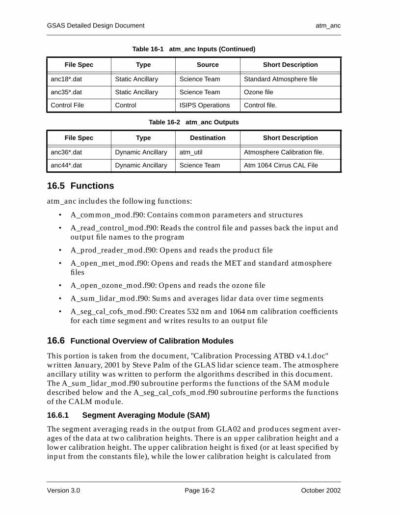
GSAS Detailed Design Document atm_anc
16.5 Functions
atm_anc includes the following functions:
• A_common_mod.f90: Contains common parameters and structures
• A_read_control_mod.f90: Reads the control file and passes back the input and output file names to the program
• A_prod_reader_mod.f90: Opens and reads the product file
• A_open_met_mod.f90: Opens and reads the MET and standard atmosphere files
• A_open_ozone_mod.f90: Opens and reads the ozone file
• A_sum_lidar_mod.f90: Sums and averages lidar data over time segments
• A_seg_cal_cofs_mod.f90: Creates 532 nm and 1064 nm calibration coefficients for each time segment and writes results to an output file
16.6 Functional Overview of Calibration Modules
This portion is taken from the document, "Calibration Processing ATBD v4.1.doc" written January, 2001 by Steve Palm of the GLAS lidar science team. The atmosphere ancillary utility was written to perform the algorithms described in this document. The A_sum_lidar_mod.f90 subroutine performs the functions of the SAM module described below and the A_seg_cal_cofs_mod.f90 subroutine performs the functions of the CALM module.
16.6.1 Segment Averaging Module (SAM)
The segment averaging reads in the output from GLA02 and produces segment aver-ages of the data at two calibration heights. There is an upper calibration height and a lower calibration height. The upper calibration height is fixed (or at least specified by input from the constants file), while the lower calibration height is calculated from
anc18*.dat Static Ancillary Science Team Standard Atmosphere file
anc35*.dat Static Ancillary Science Team Ozone file
Control File Control ISIPS Operations Control file.
Table 16-2 atm_anc Outputs
File Spec Type Destination Short Description
anc36*.dat Dynamic Ancillary atm_util Atmosphere Calibration file.
anc44*.dat Dynamic Ancillary Science Team Atm 1064 Cirrus CAL File
Table 16-1 atm_anc Inputs (Continued)
File Spec Type Source Short Description
Version 3.0 Page 16-2 October 2002
atm_anc GSAS Detailed Design Document
Figure 16-1 Process Flow Diagram
October 2002 Page 16-3 Version 3.0

GSAS Detailed Design Document atm_anc
the minimum average signal between 8 and 15 km. SAM also eliminates profiles that are cloud contaminated from the segment average (this only applies to the lower cal-ibration height). The steps (directly from the ATBD) are given below:
1) Construct a 1 Hz continuous profile of P’ from –1 to 41 km for the 532 chan-nel and from –1 to 20 km for the 1064 channel.
2) Add the background to ‘summing’ variables for each channel
3) Sum the P’532 data from H1 to H2 km and add it to a ‘summing’ variable. The values of H1 and H2 will be roughly 29 and 31, respectively, but will be changeable and read in from the constants file. Increment an ‘upper counter’.
4) Check for clouds from 22 km to 8 km above ground. If clouds were not found for this second, then do the following (number 5 below):
5) Add the 1 Hz data (each bin) between 8 and 15 km to a ‘summing’ array for each channel. Increment a ‘lower counter’.
6) If you have been doing this for t minutes, where t is read in from the con-stants file (default value: t=10), and at least 50 percent of the expected num-ber of seconds have been summed (based on the ‘upper counter’), then do the following:
- compute the average 532 signal from H1 to H2 km for the entire ‘t’ minute segment. Call this P2(532) from the sum generated in step 3 above.
- If the ‘lower counter’ exceeds 50 percent of the expected number of sec-onds, then perform c, d, and e below. Otherwise, set P1(532) and P1(1064) to invalid and skip c, d and e. This effectively means that clouds have made calculations impossible at the lower height.
- Compute the average 532 and 1064 profiles between 15 and 8 km from the summing array produced in steps 4 and 5 above.
- Find the height of the minimum in the 532 average profile between 8 and 15 km call this hmin – this is the lower calibration height
- Compute the average of the data between hmin+D and hmin-D km for both the 532 and 1064 channels, where D is in km and is read from the constants file (default = 1km). Call these P1(532) and P1(1064).
- Compute the average background for the segment for each channel call these B532 and B1064
- Output to a structure: P1(532), P1(1064), P2(532), B532, B1064, hmin, D, H1, H2 and: the latitude, longitude and time at ‘m’ points along the seg-ment, where m is a variable read from the constants file, not to exceed 30. A default value for m is 20. These points would be t/m minutes apart.
Version 3.0 Page 16-4 October 2002

atm_anc GSAS Detailed Design Document
7) 1. If after ‘t’ minutes, less than 50 percent of the expected number of sec-onds have been summed (based on the ‘upper counter’), then output miss-ing values (invalid) for P1(532), P1(1064), P2(532), B532, B1064, and the other output described in 6g above.
8) Zero out summing variables, summing array and counters
9) Process next ‘t’ minute segment in the same manner
16.6.2 CALibration Module (CALM)
The function of CALM is to compute the calibration constant for each of the segments output by SAM. The following steps summarize the process:
1) Read in the output from the segment averaging utility (run after GLA02 completes). This output contains segment averages (maybe 20-30 per gran-ule) at the two calibration heights. For each segment average, there is maybe 10-20 latitude/longitude pairs (these are the m points along the orbit segment, described in 6g above). NOTE: If the SAM and CALM mod-ules are combined into one module, obviously this step is skipped.
2) For each segment that has a valid (not invalid) P1(532), P1(1064) or P2(532) do steps 3-6 below. If all 3 of these are invalid, then there is no need to per-form steps 3-6, below. In this case, we set the 3 calibration values to invalid and skip to step 9 below)
3) At each lat/lon point, compute the average attenuated molecular backscat-ter at the two calibration heights using ATBD equations 3.2.5 and 3.2.11 (here average means a vertical average – nominally 2 km). This requires access to the MET data at that lat/lon.
4) At each lat/lon point, compute the ozone transmission from the top of the atmosphere to the calibration height (ATBD, equation 3.2.8).
5) Compute the average attenuated molecular backscatter for the segment at the two calibration heights and the average ozone transmission for the seg-ment (average of the values calculated in steps 3 and 4).
6) Compute the calibration constant as the ratio of the segment signal average to the average attenuated molecular backscatter times the average ozone transmission (ATBD, equation 3.2.6).
7) Repeat steps 2-6 for each of the 20-30 segment averages. This will yield 20-30 of the following: C1(532) – the lower 532 calibration constant, C1(1064) – the 1064 calibration constant and C2(532) – the upper 532 calibration con-stant.
8) For each segment, write out to a file the following: 1) The start and end time for the segment, 2) the 3 calibration values (532 upper and lower, and 1064 lower), 3) the standard deviations of the C values (s1(532), s1(1064) and s2(532)), 4) the three segment signal averages (532 upper and lower, 1064 lower), 5) the segment average attenuated molecular backscatter at the two calibration heights, 6) the segment average ozone transmission from the top
October 2002 Page 16-5 Version 3.0

GSAS Detailed Design Document atm_anc
of the atmosphere to the calibration height, 7) the center height and thick-ness of the upper calibration zone, 8) the center height and thickness of the lower calibration zone, 9) the segment average 532 background (B532). Note that if calibration points are thrown out during step 8 above, they are still output to the file, but have the value of ‘invalid’.
Version 3.0 Page 16-6 October 2002

Section 17
GLAS_Meta
17.1 Function
GLAS_Meta is a utility GSAS PGE. It will read product header records and the ANC45 metadata input files to create inventory-level EOS metadata files.
17.2 Design Approach
The following design criteria are specific to GLAS_Meta
• With the exception of ReadData, GLAS_Meta fully uses the standard routines from the model GSAS PGE.
• Only the header information is read from the product files.
17.3 Input and Output Files
Table 17-1 lists the required inputs to GLAS_Meta. Table 17-2 lists the outputs created by GLAS_Meta. See the GLAS Data Products Specifications Volumes or GLAS Sci-ence Data Management Plan for details regarding the these files...
Table 17-1 GLAS_Meta Inputs
File Spec Type Source Short Description
gla*.dat GLAS Products GSAS GLAS product files.
anc45*.dat Static Ancillary Science Team Product metadata input files.
anc04*.dat Dynamic Ancillary UTexas IERS Polar Motion and Earth Rotation Data File.
anc46*_0004.dat Static Ancillary Science Team Ancillary metadata input file for ANC09.
anc08*.dat Dynamic Ancillary UTexas Precision Orbit file.
anc46*_0008.dat Static Ancillary Science Team Ancillary metadata input file for ANC08.
anc09*.dat Dynamic Ancillary UTexas Precision Attitude file.
anc46*_0009.dat Static Ancillary Science Team Ancillary metadata input file for ANC09.
anc20*.dat Dynamic Ancillary UTexas Predicted orbit file.
anc46*_0020.dat Static Ancillary Science Team Ancillary metadata input file for ANC20.
anc22*.dat Dynamic Ancillary ISIPS Track file.
October 2002 Page 17-1 Version 3.0

GSAS Detailed Design Document GLAS_Meta
anc46*_0022.dat Static Ancillary Science Team Ancillary metadata input file for ANC22.
anc25*.dat Dynamic Ancillary Science Team GPS/UTC conversion file.
anc46*_0025.dat Static Ancillary Science Team Ancillary metadata input file for ANC25.
anc33*.dat Dynamic Ancillary Science Team UTC time conversion file.
anc46*_0033.dat Static Ancillary Science Team Ancillary metadata input file for ANC33.
anc37*.dat Dynamic Ancillary UTEXAS Spacecraft CG file.
anc46*_0037.dat Static Ancillary Science Team Ancillary metadata input file for ANC37.
anc39*.dat Dynamic Ancillary UTEXAS GPS file.
anc46*_0039.dat Static Ancillary Science Team Ancillary metadata input file for ANC39.
anc07*_0001.dat Static Ancillary Science Team GLAS global constants file.
Control File Control ISIPS Operations Control file.
Table 17-2 GLAS_Meta Outputs
File Spec Type Destination Short Description
gla*.met Metadata ECS ECS-compliant metadata inven-tory files.
anc04*.met Metadata ECS IERS Polar Motion and Earth Rotation metadata File.
anc08*.met Metadata ECS Precision Orbit metadata file.
anc09*.met Metadata ECS Precision Attitude metadata file.
anc20*.met Metadata ECS Predicted orbit metadata file.
anc22*.met Metadata ECS Track metadata file.
anc25*.met Metadata ECS GPS/UTC conversion metadata file.
anc33*.mett Metadata ECS UTC time conversion metadata file.
anc37*.met Metadata ECS Spacecraft CG metadata file.
Table 17-1 GLAS_Meta Inputs (Continued)
File Spec Type Source Short Description
Version 3.0 Page 17-2 October 2002
GLAS_Meta GSAS Detailed Design Document
17.4 GLAS_Meta
The basic processing algorithm for GLAS_Meta is summarized below:
• Initialize (MainInit)
• Set the local execution flags (eCntrl_Init)
• Parse the Control File (GetControl)
• Open the specified files (OpenFiles)
• Print the control file (Print_Cntl)
• Read ancillary files (ReadAnc)
• Write version info (Write_LibVer, Write_AncVer)
• Loop through available Product and Ancillary Types...
- Parse header and control data using appropriate ANC45/46 information to create inventory-level metadata.
• Close all files and generate summaries (MainWrap)
17.4.1 PGE Core Routines
PGE core routines are used exactly as defined in the Core PGE Section of this docu-ment.
• MainInit
• eCntrl_Init
• GetControl
• OpenFiles
• Print_Cntl
• Write_LibVer
• ReadANC
• Write_AncVer
• MainWrap
anc39*.met Metadata ECS GPS metadata file.
anc06*.txt Dynamic Ancillary ISIPS Operations Standard metadata/processing log file.
Table 17-2 GLAS_Meta Outputs (Continued)
File Spec Type Destination Short Description
October 2002 Page 17-3 Version 3.0

GSAS Detailed Design Document GLAS_Meta
17.4.2 Metadata Processing
The process of creating metadata files first begins with the GSAS library routines. Based on input file availability, the readGLAxx subroutine reads input product/ancillary header records and control information and parses the data into common and local header data structures. The common header data structure is further sub-setted into a metadata substructure by matching header keywords with keywords found in the appropriate ANC45/46 file. The header is parsed in a very specific way. It is important to note that the first keyword found which does not match a keyword in the ANC45/46 files causes the rest of the header information to be stored in the common_header data structure (NOT in the metadata substructure). It is critical that the metadata information within the product headers be contiguous and consistent with the ANC45/ANC46 files. Inconsistency will prevent the metadata information from being filled correctly.
After the header information is parsed, WriteMetaFile walks through the ANC45/ANC46 keywords and finds appropriate values from the header metadata substruc-ture. It then replaces default values found in the ANC45/ANC46 file with actual val-ues contained within the product headers. It writes the keywords and values in a format specific to EOS inventory-level metadata.
Version 3.0 Page 17-4 October 2002

Section 18
GLAS_APID
GLAS_APID is a utility GSAS PGE. It will read ANC29, ANC32, and/or GLA00 APID files and create tab-delimited text output files of the data. Currently, the only APID supported is APID19. Future versions of this utility will provide support for APID12 and APID13.
18.1 Function
GLAS_APID creates tab-delimited text output files for ANC29, ANC32 and APID19. The APID19 data are split among multiple files, the data being separated by sub-packet type.
18.2 Design Approach
The following design criteria are specific to GLAS_APID
• With the exception of ReadData, GLAS_APID fully uses the standard routines from the model GSAS PGE.
• Output files are named by adding extensions to the input file name.
• Multiple-input files (of differing types) is supported. Multiple-granule input is not supported since APID19 output granules must be multiple-granule.
• All products are output at one record per 1 sec. Only the first of the 40/second shot times is output in APID19.
18.3 Input and Output Files
Table 18-1 lists the required inputs to GLAS_APID. Table 18-2 lists the outputs cre-ated by GLAS_APID. See the GLAS Data Products Specifications Volumes or GLAS Science Data Management Plan for details regarding the these files. Those files which are only required by specific subsystems are noted within the table..
Table 18-1 GLAS_APID Inputs
File Spec Type Source Short Description
gla00*_19.dat Level-0 APID19 EDOS GLAS Level-0 APID19 files.
anc07*_00.dat Static Ancillary Science Team GLAS error file.
anc07*_01.dat Static Ancillary Science Team GLAS global constants file.
anc29*.dat Dynamic Ancillary GLAS_L1A Index file correlating APID times.
October 2002 Page 18-1 Version 3.0

GSAS Detailed Design Document GLAS_APID
18.4 GLAS_APID
The basic processing algorithm is summarized below:
• Initialize (MainInit)
• Set the local execution flags (eCntrl_Init)
• Parse the Control File (GetControl)
• Open the specified files (OpenFiles)
• Print the control file (Print_Cntl)
• Read ancillary files (ReadAnc)
• Write version info (Write_LibVer, Write_AncVer)
anc32*.dat Dynamic Ancillary GLAS_L1A GPS time correction file used for precision timing of GLAS data.
Control File Control ISIPS Operations Control file.
Table 18-2 GLAS_APID Outputs
File Spec Type Destination Short Description
gla00*_19.dat.time.txt
Tab-delimited text. User Time-related APID19 parame-ters.
gla00*_19.dat.ac.txt
Tab-delimited text. User Altimeter-digitizer-related APID19 parameters.
gla00*_19.dat.pc.txt
Tab-delimited text. User Photon-counter-related APID19 parameters.
gla00*_19.dat.cd.txt
Tab-delimited text. User Cloud digitizer-related APID19 parameters.
gla00*_19.dat.time.txt
Tab-delimited text. User Time-related APID19 parame-ters.
gla00*_19.dat.gps.txt
Tab-delimited text. User GPS-related APID19 parame-ters.
gla00*_19.dat.ct.txt Tab-delimited text. User C&T-related APID19 parame-ters.
anc29*.dat.txt Tab-delimited text. Users Index file parameters.
anc32*.dat.txt Tab-delimited text. Users GPS time correction parame-ters.
anc06*.dat Dynamic Ancillary ISIPS Operations Standard metadata/processing log file.
Table 18-1 GLAS_APID Inputs (Continued)
File Spec Type Source Short Description
Version 3.0 Page 18-2 October 2002

GLAS_APID GSAS Detailed Design Document
• Write requested ANC29 data
• Write requested ANC32 data
• Loop through available APID Types...
- If APID is input, ProcessAPID
• Close all files and generate summaries (MainWrap
18.4.1 PGE Core Routines
PGE core routines are used exactly as defined in the Core PGE Section of this docu-ment.
• MainInit
• eCntrl_Init
• GetControl
• OpenFiles
• Print_Cntl
• Write_LibVer
• ReadANC
• Write_AncVer
• MainWrap
October 2002 Page 18-3 Version 3.0

GSAS Detailed Design Document GLAS_APID
Version 3.0 Page 18-4 October 2002

Appendix A
Processing Scenarios
All identified scenarios that will be eventually tested.
Table A-1 Reprocessing Scenarios
Scenario Input Output Dependencies Processes
End to end Lidar Level 0, ANC data (POD, Met, Cal file), Cntrl
GLA02, 7-11, Meta-data
L1A Atm ATBD, L1B Atm ATBD, L2 Atm ATBD, POD interp, Met interp
End to end Altime-ter
Level 0, POD, PAD, Met, Cal file, Cntrl
GLA05,6,12-15, Meta-data
L1A Altimeter ATBD, L1B Waveform ATBD, L1B Elevation, L2 Elevation, POD, PAD, Geoloc
Level 1A Altimeter Level 0, Cal file, Cntrl GLA01, Metadata
L1A Altimeter ATBD
Level 1B Waveform GLA01, POD, PAD, Cal file, ANC 19, surf_type_grid, Cntrl
GLA05,Metadata
L1B Waveform ATBD, POD, PAD, Geoloc, surf_type interp
Level 1B Elevation GLA05, GLA09&11 (if avail), tide coeff, geoid, ANC 12, DEM, Met
GLA06, Metadata
Geoid, Tides, Geoloc, Met, DEM interp, Instr Range Cor (5) Reflectance, Atm Flag
Level 2 Elevation GLA05, GLA06, 4 Masks
GLA12-15, Metadata
Geoloc, Instr Cor Range Region-Specific Parame-ter Calculations
Waveform Algo-rithm changes (standard, ice sheet, sea ice, ocean, land)
GLA01, GLA05, Cal file GLA05, Metadata
GLA06, GLA12-15 (1 or all)
Specific Wave-form algorithm process, Geolo-cation
Replace POD and/or PAD on GLA05
GLA05, POD and/or POD
GLA05, Metadata
POD and/or PAD, Geolocation
Replace PAD and/or POD on GLA06
GLA06, PAD and/or POD
GLA06, Metadata
GLA12-15 PAD and/or POD, Geolocation
October 2002 Page A-1 Version 3.0

GSAS Detailed Design Document Processing Scenarios
Met changes, redo Met Cor
GLA06, GLA12-15, Met file
GLA06, GLA12-15, Metadata
Met Interpola-tion, Geolocation
Tides Change, redo tide cor
GLA06, GLA12-15, tide coeff
GLA06, GLA12-15, Metadata
Tide algorithms, Geolocation
Geoid changes GLA06, GlA12-15, Geoid
GLA06, GLA12-15, Metadata
Geoid
Standard Instr Cor Changes
GLA05, GLA06, GLA12-15
GLA06, GLA12-15, Metadata
Standard Instr Cor Algorithm, Geolocation
Region Spec Instr Cor Changes
GLA05, GLA06, GLA12-15
GLA06, GLA12-15, Metadata
Region Specific Instr Cor Algo-rithm
Reflectance Algo-rithm changes
GLA05, GLA06, GLA12-15
GLA06, GLA12-15, Metadata
Reflectance ATBD
Change GLA06 based on WF Algo-rithm changing for GLA05
GLA05, GLA06, GLA12-15
GLA06, GLA12-15, Metadata
Range Instr Cor Calculation, Geolocation
Replace PAD and/or POD on GLA12-15
GLA12-15, PAD and/or POD
GLA12-15, Metadata
POD and or PAD, Geolocation
Creation of GLA07 BackScatter Pro-files
GLA02, Met, POD, 400 sec avg file
GLA07, Metadata
Interp POD, Interp Met, Molec BackScat Pro-files, Calib Coeff, 1064 BackScat Profiles, 532 BackScat Profiles
Creation of GLA08 Aerosol Layers
GLA07, Constants, GLA09
GLA08 1 and 4 sec BackScat aver-ages, PBL/Aero-sol <20 km layers, 20-40 km aerosol layers
Table A-1 Reprocessing Scenarios (Continued)
Scenario Input Output Dependencies Processes
Version 3.0 Page A-2 October 2002

Processing Scenarios GSAS Detailed Design Document
Creation of GLA09 Cloud Layers
GLA07, Constants GLA09 1 and 4 sec BackScat aver-ages, Cloud Lay-ers
Creation of GLA10 Cross Section Pro-files and Creation of GLA11 Optical Depths
GLA07, GLA08, GLA09, Constants
GLA10, GLA11
Cloud Optical Properties, Aero-sol Optical Prop-erties, 1 and 4 sec BackScat averages
Table A-1 Reprocessing Scenarios (Continued)
Scenario Input Output Dependencies Processes
October 2002 Page A-3 Version 3.0

GSAS Detailed Design Document Processing Scenarios
Version 3.0 Page A-4 October 2002

Appendix B
Makefiles and Libraries
Developers are “strongly” encouraged to use standard GSAS libraries and makefiles. GSAS libraries leverage existing code to speed development and ease maintenance. Makefiles ensure common compiler flags and allow developers to deliver their soft-ware as part of a general GSAS delivery.
B.1 Compilation
Note: This documentation is specific to the GLAS development environment. It assumes that the core directory of the GLAS software is located at “/glas/vob”.
B.1.1 To compile the whole distribution
cd /glas/vob/srcmake
B.1.2 To compile only the libraries
cd /glas/vob/srcmake libs
B.1.3 To recompile a library in debug mode
cd /glas/vob/src/library_directorymake debug
B.1.4 To recompile a library in optimized mode
cd /glas/vob/src/library_directorymake fast
B.1.5 To compile a specific executable
(requires that the libraries are compiled beforehand)
cd /glas/vob/src/executable_directorymake
B.1.6 To compile a specific executable in debug mode
(requires that the libraries are compiled beforehand)
cd /glas/vob/src/executable_directorymake debug
B.1.7 To compile a specific executable in optimized mode
(requires that the libraries are compiled beforehand)
cd /glas/vob/src/executable_directorymake fast
October 2002 Page B-1 Version 3.0

GSAS Detailed Design Document Makefiles and Libraries
B.2 Using Libraries
This section details the use of libraries, both at development and run time stages.
B.2.1 Development
To use a library, you need to include the path and the library name in your Makefile. The following example shows how to use the platform_lib (which is stored in the /glas/vob/src/lib directory) to compile a test program:
f90 test.f90 -L/glas/vob/src/lib -lplatform -otest
The next example show how to use the file and anc libraries as well. (A side note: By unix convention the full filenames are libplatform.sl, libfile.sl, and libanc.sl, however when they are specified with the -l argument on the compile line, the “lib” and “.sl” parts are dropped).
f90 test.f90 -L/glas/vob/src/lib -lplatform -lanc -lfile –otest
ORDER IS IMPORTANT. See Foundation Libraries section of this document to verify that the libraries are specified in the correct order on the compile line.
B.2.2 Runtime
GSAS libraries are dynamically-linked shared libraries. What this means is that the libraries are not statically linked with executables, but dynamically linked on demand at runtime. With this in mind, it is important that the executable be able to determine the location of the libraries at runtime. During compilation, the location of the libraries is stored in the executable code. If the executable is moved, and the loca-tion is relative, the libraries will not be found upon execution. In this case, a devel-oper should use the following procedure to allow executables to link to dynamic libraries, no matter their location.
chatr +s enable <executable_name>setenv SHLIB_PATH <pathname to libraries>
This procedure tells the executable to use the SHLIB_PATH environmental variable to find its libraries, then sets that variable to the path of the shared libraries.
The other way of handling this is to link the libraries into the current directory. The executable is set to look in the current directories first for its libraries.
B.3 Some Development Hints
• If you want to use the GLAS libraries, simply compile them (as above) and include the appropriate lines in your makefile (again, as above).
• As long as you model the Makefile for your executable after that of the GLAS PGEs, you will be using shared libraries and will not need to recompile your executable after recompiling a library - unless global data structures or sub-routine arguments are changed.
Version 3.0 Page B-2 October 2002

Makefiles and Libraries GSAS Detailed Design Document
• If you would like to debug the routines in a specific library, cd to that directory and do a make clean; make debug. Next time you run your executable (you don’t have to recompile it), it will run with the debug version of the library.
• Using the –g and +check=all flags (included with make debug) is a good idea during testing.
• If you want to get fancy and create a custom makefile for a special purpose, simply use another name for the makefile and use make –f mymakefile.
• You may add custom options to the standard makefiles by putting the options on the gF90_AUX_FLAGS line. For example, if you wish to define a custom flag (DEBUG_TIME) for debugging purposes, define it as follows:
gF90_AUX_FLAGS= -DDEBUG_TIME
B.4 Makefile Details
This is an attempt to explain how GLAS makefiles work. This assumes the reader is somewhat familiar with the GLAS VOB layout.
B.5 Types of Makefiles
There are different types of makefiles. This section identifies each.
B.5.1 The Main Makefile
This makefile is located at /glas/vob/Makefile. This makefile builds all GSAS soft-ware and installs the binaries and libs in the /glas/vob/bin and /glas/vob/lib direc-tories. This makefile is primarily used during production, not development. Developers should always use/link to the binaries and libraries within the src direc-tory, not those in the /bin and /lib directories since the top-level makefile is the only one which populates such directories.
B.5.2 The src Makefile
This makefile is located at /glas/vob/src/Makefile. It is the main development makefile which will recursively build all GSAS deliverable software. There are options to:
• build all deliverable GLAS Libraries (make libs)
• build all deliverable GLAS binaries (make progs)
• build all deliverable Libraries and binaries (make all) -the default
• build all deliverable Libraries and binaries in debug mode (make debug)
• build all deliverable Libraries and binaries in optimization mode (make fast)
• clean up all object code and module files (make clean)
B.5.3 Library Makefiles
These makefiles are located at src/common_libs/*/Makefile. There are options to:
October 2002 Page B-3 Version 3.0

GSAS Detailed Design Document Makefiles and Libraries
• Compile library source and install library (make)
• Compile library source in debug mode and install library (make debug)
• Compile library source in optimization mode and install library (make fast)
The libraries are derived objects and installed into /glas/vob/src/lib
B.5.4 Subsystem Makefiles
These makefiles are located at /glas/vob/src/*_lib/Makefile (where * = l1a, atm, elev, wf)
• Compile library source and install library (make)
• Compile library source in debug mode and install library (make debug)
• Compile library source in optimization mode and install library (make fast)
The libraries are derived objects and installed into /glas/vob/src/lib. When installed, the libraries are stored in /glas/vob/lib.
B.5.5 Exec makefiles
These makefiles are located in the directory of each delivered executable: src/GLAS_L1A/Makefile, src/GLAS_L0proc/Makefile, etc. There are options to:
• Compile binary source (make)
• Compile binary source in debug mode (make debug)
• Compile binary source in optimization mode (make fast)
The executables are derived objects and installed into /glas/vob/bin.
B.6 A Sample Heavily-Commented Makefile# NAME: Makefile## FUNCTION: Makefile for GLAS_Exec## FILES ACCESSED: See TARGETS definition. # ALL DIRECTORY SPECIFICATIONS SHOULD BE RELATIVE, NOT ABSOLUTE, PATHS!!## COMMENTS: None.## HISTORY: ## 1998 December 18, JLee, Initial Version# 1999 January 14, JLee, Ported to HP # 1999 October 18, JLee Removed default DEBUG, removed recursion# 1999 October 24, JLee Set the bit to do SHLIB_PATH ##----- Set filepaths## PATHLVL is the path you use to get to /glas/vob/src, but it should# be a relative path so that we can compile outside the VOB.#PATHLVL=..
Version 3.0 Page B-4 October 2002

Makefiles and Libraries GSAS Detailed Design Document
## UTILDIR is where the GLAS makefile includes can be found. These files# contain settings specific to GLAS Makefiles.# /glas/vob/cc_util is the actual path.#UTILDIR=$(PATHLVL)/../cc_util## Include Standard GLAS Definitions #include $(UTILDIR)/make_defs.$(BRAND)include $(UTILDIR)/make_defs.incl## Define libraries we will need. They are located in /glas/vob/src/lib.# This path is pre-defined (relatively) in the GLAS include files.# The actual filename for –lwf is libwf.sl, -file is libfile.sl# LIBS= -ll1a -latm -lwf -lelev -lprod -lfile -ltime -lanc -lcntrl \-lerr –lplatform## Define the Production directory where we will copy the binary upon# creating a production build#PRODDIR=$(PATHLVL/../bin)## Define the target binary#TARGET=GLAS_Exec## Define the objects will are needed by the Target#OBJECTS= \
CntlDefs_mod.o fCntl_mod.o eCntl_mod.o \MainInit_mod.o ReadData_mod.o GetControl_mod.o \CloseFiles_mod.o OpenFiles_mod.o WriteL1A_mod.o WriteWF_mod.o \WriteAtm_mod.o WriteElev_mod.o MainWrap_mod.o \ReadAnc_mod.o L1AMgr_mod.o ElevMgr_mod.o WFMgr_mod.o AtmMgr_mod.o \vers_exec_mod.o GLAS_Exec.o
## Custom Rules#gF90_AUX_FLAGS=## Make our Target by default#all: $(TARGET)## TARGET, LIBS and OBJECTS are defined in this makefile. # LINK_EXE.f90 and FFLAGS are defined in the GLAS includes.# chart +s enable allows the executable to use the SHLIB_PATH to# look for its shared libraries.#$(TARGET): $(OBJECTS) Makefile
$(LINK_EXE.f90) $(FFLAGS) -o $(TARGET) $(OBJECTS) $(LIBS); \chatr +s enable $(TARGET)
## Include Standard GLAS Dependencies#include $(UTILDIR)/make_depends.incl
October 2002 Page B-5 Version 3.0

GSAS Detailed Design Document Makefiles and Libraries
## End of MakeFile#
Version 3.0 Page B-6 October 2002

Abbreviations & Acronyms
A2P Algorithm-to-Product Conversion
ALT Altimeter or Altimetry, also designation for the EOS-Altimeter spacecraft series
ANCxx GLAS Ancillary Data Files
APID GLAS Level-0 Data file
ATBD Algorithm Theoretical Basis Document
ATM Atmosphere
CCB Change Control Board
ClearCase GSAS version tracking software
CR Change Request
DAAC Distributed Active Archive Center
DEM Digital Elevation Model
DFD Data Flow Diagram
DLT Digital Linear Tape
EDOS EOS Data and Operations System
EDS Expedited Data Set
ELEV Elevation
EOC EOS Operating Center
EOS NASA Earth Observing System Mission Program
EOSDIS Earth Observing System Data and Information System
GB Gigabyte
GDS GLAS Ground Data System
GLAS Geoscience Laser Altimeter System instrument or investigation
GLAxx GLAS Science Data Product Files
GLOP GLAS Level-0 PGE (correctly called GLAS_L0proc)
GPS Global Positioning System
GSAS GLAS Science Algorithm Software
GSFC NASA Goddard Space Flight Center at Greenbelt, Maryland
GSFC/WFF NASA Goddard Space Flight Center/Wallops Flight Facility at Wallops Island, Virginia
October 2002 Page AB-1 Version 3.0

GSAS Detailed Design Document Abbreviations & Acronyms
HDF Hierarchal Data Format
HDF-EOS EOS-specific Hierarcial Data Format
I-SIPS Icesat Science Investigator Led Processing System
I/O Input/Output
ICESAT Ice, Cloud and Land Elevation Satellite
ID Identification
ID Identification
IEEE Institute for Electronics and Electrical Engineering
ISF Instrument Support Facility
IST Instrument Star Tracker
KB Kilobyte
L0 Level 0
L1A Level-1A
L1B Level-1 B
L2 Level-2
LASER Light Amplification by Stimulated Emission of Radiation
LASER Light Amplification by Stimulated Emission of Radiation
LIDAR Light Detection and Ranging
LIDAR Light Detection and Ranging
LPA Laser Pointing Array
LRS Laser Reference System
MB Megabyte
MET (context sensitive) Mission Elapsed Time or Meteorological
MOSS NEED DEFINITION
N/A or NA Not (/) Applicable
NASA National Aeronautics and Space Administration
NOAA National Oceanic and Atmospheric Administration
P2A Product-to-Algorithm Conversion
PAD Precision Attitude Determination
PDF Portable Document Format
PDS Production Data Set
PGE Product Generation Executable
Version 3.0 Page AB-2 October 2002

Abbreviations & Acronyms GSAS Detailed Design Document
POD Precision Orbit Determination
POD Precision Orbit Determination
PR Problem Report
QA Quality Assessment
QAP Quality Assessment Processing
SC Structure Chart
SCF Science Computing Facility
SDMP Science Data Management Plan
SDMS Scheduling and Data Management System
SDP Standard Data Products
SRS Stellar Reference System
SSMP Science Software Management Plan
SSRF Science Software Requirements Document
TBD to be determined, to be done, or to be developed
TBD to be determined, to be done, or to be developed
UNIX the operating system jointly developed by the AT&T Bell Laboratories and the University of California-Berkeley System Division
UTC Universal Time Correlation
WF Waveform
October 2002 Page AB-3 Version 3.0

GSAS Detailed Design Document Abbreviations & Acronyms
Version 3.0 Page AB-4 October 2002

Glossary
aggregate A collection, assemblage, or grouping of distinct data parts together to make a whole. It is generally used to indicate the grouping of GLAS data items, arrays, elements, and EOS parameters into a data record. For example, the collection of Level 1B EOS Data Parameters gathered to form a one-second Level 1B data record. It could be used to represent groupings of various GLAS data entities such as data items aggregated as an array, data items and arrays aggregated into a GLAS Data Element, GLAS Data Elements aggregated as an EOS Data Parameter, or EOS Data Parameters aggregated into a Data Product record.
array An ordered arrangement of homogenous data items that may either be syn-chronous or asynchronous. An array of data items usually implies the ability to access individual data items or members of the array by an index. An array of GLAS data items might represent the three coordinates of a georeference location, a collection of values at a rate, or a collection of values describing an altimeter waveform.
file A collection of data stored as records and terminated by a physical or logical end-of-file (EOF) marker. The term usually applies to the collection within a storage device or storage media such as a disk file or a tape file. Loosely employed it is used to indicate a collection of GLAS data records without a standard label. For the Level 1A Data Product, the file would constitute the collection of one-second Level 1A data records generated in the SDPS work-ing storage for a single pass.
header A text and/or binary label or information record, record set, or block, prefacing a data record, record set, or a file. A header usually contains identifying or descriptive information, and may sometimes be embedded within a record rather than attached as a prefix.
item Specifically, a data item. A discrete, non-decomposable unit of data, usually a single word or value in a data record, or a single value from a data array. The representation of a single GLAS data value within a data array or a GLAS Data Element.
label The text and/or binary information records, record set, block, header, or head-ers prefacing a data file or linked to a data file sufficient to form a labeled data product. A standard label may imply a standard data product. A label may consist of a single header as well as multiple headers and markers depending on the defining authority.
Level 0 The level designation applied to an EOS data product that consists of raw instrument data, recorded at the original resolution, in time order, with any duplicate or redundant data packets removed.
Level 1A The level designation applied to an EOS data product that consists of recon-structed, unprocessed Level 0 instrument data, recorded at the full resolution with time referenced data records, in time order. The data are annotated with ancillary information including radiometric and geometric calibration coeffi-cients, and georeferencing parameter data (i.e., ephemeris data). The included, computed coefficients and parameter data have not however been applied to correct the Level 0 instrument data contents.
October 2002 Page GL-1 Version 3.0

GSAS Detailed Design Document Glossary
Level 1B The level designation applied to an EOS data product that consists of Level 1A data that have been radiometrically corrected, processed from raw data into sensor data units, and have been geolocated according to applied georefer-encing data.
Level 2 The level designation applied to an EOS data product that consists of derived geophysical data values, recorded at the same resolution, time order, and geo-reference location as the Level 1A or Level 1B data.
Level 3 The level designation applied to an EOS data product that consists of geo-physical data values derived from Level 1 or Level 2 data, recorded at a tem-porally or spatially resampled resolution.
Level 4 The level designation applied to an EOS data product that consists of data from modeled output or resultant analysis of lower level data that are not directly derived by the GLAS instrument and supplemental sensors.
metadata The textual information supplied as supplemental, descriptive information to a data product. It may consist of fixed or variable length records of ASCII data describing files, records, parameters, elements, items, formats, etc., that may serve as catalog, data base, keyword/value, header, or label data. This data may be parsable and searchable by some tool or utility program.
orbit The passage of time and spacecraft travel signifying a complete journey around a celestial or terrestrial body. For GLAS and the EOS ALT-L spacecraft each orbit starts at the time when the spacecraft is on the equator traveling toward the North Pole, continues through the equator crossing as the space-craft ground track moves toward the South Pole, and terminates when the spacecraft has reached the equator moving northward from the South Polar region.
model A graphical representation of a system.
module A collection of program statements with four basic attributes: input and output, function, mechanics and internal data.
parameter Specifically, an EOS Data Parameter. This is a defining, controlling, or con-straining data unit associated with a EOS science community approved algo-rithm. It is identified by an EOS Parameter Number and Parameter Name. An EOS Data Parameter within the GLAS Data Product is composed of one or more GLAS Data Elements
pass A sub-segment of an orbit, it may consist of the ascending or descending por-tion of an orbit (e.g., a descending pass would consist of the ground track seg-ment beginning with the northernmost point of travel through the following southernmost point of travel), or the segment above or below the equator; for GLAS the pass is identified as either the northern or southern hemisphere por-tion of the ground track on any orbit
PDL Program Design Language (Pseudocode). A language tool used for module programming and specification. It is at a higher level than any existing com-pilable language.
process An activity on a dataflow diagram that transforms input data flow(s) into output data flow(s).
Version 3.0 Page GL-2 October 2002

Glossary GSAS Detailed Design Document
product Specifically, the Data Product or the EOS Data Product. This is implicitly the labeled data product or the data product as produced by software on the SDPS or SCF. A GLAS data product refers to the data file or record collection either prefaced with a product label or standard formatted data label or linked to a product label or standard formatted data label file. Loosely used, it may indicate a single pass file aggregation, or the entire set of product files con-tained in a data repository.
program The smallest set of computer instructions that can be executed as a stand-alone unit
record A specific organization or aggregate of data items. It represents the collection of EOS Data Parameters within a given time interval, such as a one-second data record. It is the first level decomposition of a product file.
Scenario A single execution path for a process.
Standard Data Product
Specifically, a GLAS Standard Data Product. It represents an EOS ALT-L/GLAS Data Product produced on the EOSDIS SDPS for GLAS data product generation or within the GLAS Science Computing Facility using EOS science community approved algorithms. It is routinely produced and is intended to be archived in the EOSDIS data repository for EOS user community-wide access and retrieval.
State Transition Diagram
Graphical representation of one or more scenarios.
Stub (alias dummy module) a primitive implementation of a subordinate module, which is normally used in the top-down testing of superordinate (higher) mod-ules.
Structure Chart A graphical tool for depicting the partitioning of a system into modules, the hierarchy and organization of those modules, and the communication inter-faces between the modules.
Structured Design The development of a blueprint of a computer system solution to a problem, having the same components and interrelationships amount the components as the original problem has.
Subroutine A program that is called by another program
variable Usually a reference in a computer program to a storage location, i.e., a place to contain or hold the value of a data item.
October 2002 Page GL-3 Version 3.0

GSAS Detailed Design Document Glossary
Version 3.0 Page GL-4 October 2002