1

Growth Rate and Level Effects, the Adjustment of Capacity to Demand and the Sraffian

Supermultiplier

Franklin Serrano and Fabio Freitas

Instituto de Economia, Federal University of Rio de Janeiro, Brazil (IE-UFRJ)

Resumo

O artigo apresenta uma versão formal simples, porém completa, do modelo do Supermultiplicador

Sraffiano. Neste modelo o crescimento econômico é liderado pelos componentes autônomos da demanda

que não geram capacidade, o investimento privado produtivo é um gasto induzido e a distribuição de

renda é determinada exogenamente. O artigo mostra que os principais resultados em termos de efeitos

nível e taxa (de crescimento) obtidos com base nas versões do modelo com ajustamento incompleto

(longo prazo) e completo da capacidade produtiva à demanda são muito similares. Em seguida são

analisadas as condições suficientes de estabilidade dinâmica que garantem a tendência ao ajustamento

completo da capacidade produtiva à demanda e a partir das quais podemos estabelecer um limite superior

para a taxa de crescimento liderada pela demanda de acordo com o modelo. Na sequência, a literatura

crítica ao modelo é revisada, mostrando que o modelo tem sido incorretamente interpretado como sendo

um modelo de crescimento com restrição de oferta e que esta leitura incorreta do modelo levou a uma

confusão entre, de um lado, a análise da convergência das taxa de crescimento da economia para um valor

exógeno da taxa garantida harrodiana com a demanda ajustada à capacidade produtiva e, de outro, a

análise oposta da tendência de ajustamento da capacidade produtiva à demanda, em que a taxa garantida

de crescimento se ajusta endogenamente ao ritmo de expansão da demanda agregada.

Abstract

The paper presents a very simple but complete formal version of the sraffian supermultiplier model in

which growth is led by the autonomous components of demand that do not create capacity, private

productive investment is induced and distribution is exogenous. We show that the main results of the long

period and fully adjusted versions of the model in terms of growth rate and level effects are quite similar

and thus such results in no way require the full adjustment of capacity to demand. We then analyze a

simple set of sufficient dynamic local stability conditions that allows the long period positions to gravitate

towards the fully adjusted positions in which capacity is adjusted to demand and also provide the upper

limit to demand led growth paths. We then show how some critics of the model have misinterpreted the

model as being supply led and how this led to a further confusion between the analysis of the tendency

toward a constant value of the capacity saving determined Harrodian warranted rate of growth and the

proper stability analysis of the opposite process of adjusting capacity to demand (which tends to adjust

the warranted rate endogenously to the growth rate of autonomous demand).

Key words: Effective Demand; Growth; Supermultiplier

Palavras Chave: Demanda Efetiva; Crescimento; Supermultiplicador

Códigos JEL (JEL Codes) : E11; E12; O41

Área 6 - Crescimento, Desenvolvimento Econômico e Instituições

2

I. Introduction

The paper presents a very simple but complete formal version of the sraffian supermultiplier model

(Serrano, 1995 and 1996) in which growth is led by the autonomous components of demand that do not

create capacity (autonomous consumption in this case), productive investment is induced and distribution

is exogenous. We show that in this model changes in the trend rate of growth of autonomous consumption

have a permanent effect on the trend rates of growth of output and capacity while changes in the

determinants of the marginal propensity to consume (such as income distribution) or in the exogenous

parameters of the marginal propensity to invest only have a persistent level effect on both output and

productive capacity. We note that quite similar results are obtained both in the long period and fully

adjusted versions of the supermultiplier. In the long period positions, discussed in section II, we take the

investment share (marginal propensity to invest) as given. This makes aggregate demand and capacity

tend to grow at the same rate, while at the same time the level of the actual degree of capacity utilization

remains endogenous. The fully adjusted positions, which we use to study the slower process by which the

marginal propensity to invest gradually changes endogenously as a reaction to discrepancies between the

actual and the planned degrees of capacity utilization and make also the levels of capacity output adjust to

the levels of demand, are the subject of the next three sections. In section III we discuss the gravitation of

the actual degree of capacity utilization towards the exogenous normal (or planned) degree. In section IV

we provide a set of sufficient formal conditions for the dynamic stability of the process of adjusting

capacity to demand, discuss the economic meaning of these conditions and in particular their implications

for the precise characterization of the limits to demand led growth paths. Then in section V we present the

main results of the fully adjusted final equilibrium model. Equipped with these results we then use

sections VI to address the criticisms of the sraffian supermultiplier found in the literature. We show how

the model has been misinterpreted and how that the related mathematical “stability” analysis of the model

presented by some of the critics actually concerns the time path of the supply led warranted equilibrium

growth rate in which investment is determined by capacity saving and has nothing to do with the

conditions for the dynamic stability of the sraffian supermultiplier demand led growth model..The paper

finishes with Section VII that contains some final remarks.

II. The supermultiplier and the long period position

We shall present the sraffian supermultiplier growth model in its simplest possible form in order to

facilitate the identification of the most relevant properties of the model. Hence, we assume a closed

capitalist economy without an explicit government sector. The only method of production in use requires

a fixed combination of homogeneous labor input with homogeneous fixed capital to produce a single

homogeneous output. Natural resources are supposed to be abundant and constant returns to scale and no

technological progress are also assumed. We also assume that growth is not constrained by labor scarcity.

In this very simple analytical context, the level of capacity output1 of the economy depends on the

existing level of capital stock available and on the technical capital-output ratio according to the

following expression:

(

)

(1)

where is the level of the capacity output of the economy, is the level of capital stock installed in

the economy and is the technical capital-output ratio. Since is given, then the rate of growth of

capacity output is equal to the rate of capital accumulation

1 All variables are measured in real terms. Moreover, output, income, profits, investment and savings are all presented in gross terms. The

formal analysis will be made using continuous time for mathematical convenience.

3

( ⁄

)

(2)

where is rate of capital accumulation, ⁄ is the actual degree of capacity utilization defined

as the ratio of the current level of aggregate output ( ) to the current level of capacity output, ⁄ is the

investment share in aggregate output defined as the ratio of gross aggregate investment ( ) to the level of

gross aggregate output, and is the capital drop-out ratio which is exogenously determined.2 According

to equation (2) the rate of capital accumulation depends on the behavior of the actual degree of capacity

utilization and of the investment share.3 Given the technical capital-output ratio, the change of the actual

degree of capacity utilization through time is then described by the difference between the rate of growth

of output and the rate of capital accumulation following the differential equation below:

( ) (3)

where is the rate of growth of aggregate output.

Aggregate income in the model is distributed in the form of wages and profits. We shall assume that

besides the single technique in use, income distribution (either the normal real wage or the normal rate of

profits) is also given exogenously along classical (sraffian) lines. We accordingly assume that there is free

competition and that output (but not capacity) adjusts fairly quickly to effective demand such that that

market prices are equal to a normal price that yields a uniform rate of profits on capital using the

dominant technique when the degree of capacity utilization is equal to the normal or planned degree

.4 Note that we can make the assumption of normal prices at this stage of our analysis even when we are

dealing with situations in which the actual degree of capacity utilization can be quite different from the

normal/planned degree because under classical competition existing individual firms will not have the

power to sustain persistently higher (than normal) market prices if the actual degree of capacity utilization

of a particular firm is below (or very much above) 5

the normal or planned level and thus their actual unit

costs are higher than normal. Indeed, at higher than normal prices other firms already in the market may

be operating at the planned degree of utilization and can easily increase their market shares by

undercutting the firm (or firms) that has raised prices above the normal price. Moreover, these higher

prices may also attract new entrants to the market which would also be able to operate their appropriately

sized new capacities at the planned degree of utilization and reap higher than normal profits by

undercutting the incumbent firm (or firms) that has raised prices to pass on their higher than normal actual

average costs to market prices. Thus, both actual and potential competition of existing and/or new firms

would ensure that effective demand will be met at the normal price even if the actual degree of capacity

utilization is quite different from the normal or planned degree.6

Since we are assuming that output adapts quickly to demand, the level of output is determined by

aggregate demand at the normal price. Effective demand is composed of real aggregate consumption and

gross real aggregate investment. We assume that capitalist firms undertake all investment expenditures in

2 The equation of capital accumulation is derived from the equation that defines the level of aggregate gross fixed investment.

Dividing both sides of the equation by we obtain ⁄ . Solving this last equation for the rate of capital accumulation gives us

( ⁄ ) ( ⁄ )( ⁄ )( ⁄ ) (( ⁄ ) ⁄ ) . 3 This equation and the understanding that it is raising the investment share in capacity output rather than in actual output that increases the

rate of growth of capacity output and that these two shares can be quite different if the actual degree of capacity utilization can be different

than the normal or planned degree appears to have been put forward first by Garegnani(2014 [1962]). 4 We interpret the normal or planned degree of capacity utilization following Ciccone(1986,1987) as determined, among other things, by an

exogenous historical/conventional ratio of average to peak demand which, presumably being based on the observation of the actual cyclical

pattern of the market over a very long period of time, is assumed to be exogenous and not affected at all by current oscillations of demand. 5 If the actual degree of utilization is below the normal degree fixed cost per unit of output will be higher than normal. If the degree of

utilization is just above the normal degree unit costs will keep falling (giving rise to extra profits at normal prices) until at degrees of capacity

utilization very much above the normal degree there cost will begin to rise due to the extra costs involved in operating capacity way above

its cost minimizing range (Ciccone (1987)). 6 Normal prices are thus a kind of entry preventing “limit prices” in the language of the old industrial organization literature. Many Sraffians

make the same argument in terms of a presumption of a uniformity of expected rates of profit on new investment (Garegnani, 1992);

Ciccone, 1986 and 2011) but we think that our reasoning in terms of existing producers is much simpler.

4

the economy.7 Aggregate consumption is composed of an autonomous component and an induced

component (with ) being the marginal propensity to consume, given by consumption habits

and the given distribution of income. Thus is the given aggregate marginal propensity to save.

Let us now suppose in addition to the existence of a positive level of autonomous consumption that the

level of aggregate investment is an induced expenditure according to the following expression

(4)

where (with ) is the marginal propensity to invest of capitalist firms, which we assume,

provisionally, to be determined exogenously.

Since we are thinking of a demand led system, we assume that the marginal propensity to spend is

strictly lower than one (if it was equal to one we would have Say´s law).8 In addition we are at the same

time assuming that there is a positive level of autonomous consumption (financed by credit or by the

monetization of accumulated wealth), otherwise no positive level of output could be sold profitably.

This gives us the demand determined level of output in a long period position as:

(

)

(5)

where the term within the parenthesis is the supermultiplier that captures the effects on the level of output

associated with both induced consumption and investment.9

In this simple framework, given the existence of autonomous consumption expenditures we have that the

marginal propensity to save does not determine the actual savings ratio (the average propensity to save).

The saving ratio is instead determined by and equal to the marginal propensity to invest as

(6)

where ( )⁄ what Serrano (1996) called “the fraction”, the ratio between the average and

the marginal propensities to save ( ⁄ ) .10 With positive levels of autonomous consumption (i.e.,

), it follows that and ⁄ . Therefore, the given marginal propensity to save defines

only the upper limit to the value of the average saving ratio of the economy corresponding to a given

marginal propensity to save. In this case, the saving ratio depends not only on the marginal propensity to

save but also on the proportion between autonomous consumption and investment. Thus, an increase

(decrease) in the levels of aggregate investment in relation to autonomous consumption leads to an

increase (decrease) in the saving ratio. As a result, the existence of a positive level of autonomous

consumption is sufficient to make the saving ratio an endogenous variable.

In this context, for a given level of income distribution and, hence, a given marginal propensity to

save, a given marginal propensity to invest (equal to the investment share of output) uniquely

determines the saving ratio of the economy. Hence an exogenous increase (decrease) in the investment

7 Thus, there is no residential investment in our simplified model. 8 Neo-Kaleckians call this assumption “keynesian stability” (see, for example, Lavoie, 2013 and Allain 2013). But in fact it is much more

than that. It is actually what we mean when we say that output is demand determined. For if the marginal propensity to spend were equal to

one and there no autonomous demand we would have Say´s law and if the marginal propensity to spend was lower than one but with no

autonomous demand the economy would collapse and output would fall to zero. In this connection, see Serrano (1995,1996) and Lopez &

Assouz (2010, chapter 2).. 9 See for details on the marginal propensity to consume Serrano (1995,1996) and on the (not fully adjusted) long period supermultiplier with

a given marginal propensity to invest Serrano (2001), and Cesaratto, Serrano &Stirati (2003). 10 Observe that according to (6) if there were no autonomous consumption (i.e., ) then we would have and ⁄ .. Note

also that, in this extreme case, if income distribution is exogenously given, then the marginal propensity to save determines the saving ratio

and the investment share in output.

5

share of output in relation to the marginal propensity to save would raise (reduce) the fraction , and,

therefore, would cause a decrease (an increase) in the ratio of autonomous consumption to output ⁄

and an increase (a decrease) in the saving ratio.

Now let us suppose that autonomous consumption grows at an exogenously determined rate

. Since the marginal propensities to consume and to invest are given exogenously, the

supermultiplier is also exogenous and constant. Therefore, aggregate output, induced consumption and

investment grow at the same rate as autonomous consumption. The capital stock also tends to grow at this

same rate since its trend rate of growth is governed by the growth rate of gross investment. The fact that

the rate of growth of the stock of capital follows the rate of growth of gross investment can be shown as

follows. From the definitional equation we can obtain the differential equation ( )( ) relating the rate of growth of the flow of gross investment to the rate of capital

accumulation (the rate of growth of the stock of capital). From this differential equation it can be seen

that, if initially the rate of capital accumulation is different from the rate of growth of investment, the rate

of capital accumulation begin to change towards the rate at which investment grows. We can also see that

the rate of capital accumulation only becomes constant when it becomes equal to the given rate of growth

of gross investment growth rate.11

In the context of our model with a given marginal propensity to invest,

this implies that capacity output tend to grow at the same rate as autonomous consumption. Moreover, the

actual degree of capacity utilization will tend to a constant value as can be calculated from equation (3)

above and its trend level can be determined using equation (2) as follows12

:

( )

(7)

According to equation (7) above, given the marginal propensity to invest , a higher (lower) rate of

growth of autonomous consumption leads to a permanently higher (lower) actual degree of capacity

utilization. Moreover, for any exogenously given marginal propensity to invest, there is no reason why

the actual degree of capacity utilization should tend to its normal or planned level. So in this simplified

long period supermultiplier model the growth of capacity follows the growth of (autonomous

consumption) demand but the level of capacity may be quite different from the level of aggregate

demand.

By mere inspection of equations (5) and (7) we can deduce the most interesting results of the long period

supermultiplier model. The rate of growth of output will tend to follow the rate of growth of autonomous

consumption and the same occurs with the rates of growth of induced consumption and investment. For

its turn, the capital stock (and capacity output) will tend to follow the growth of investment and,

therefore, will also tend to grow at the rate of expansion of autonomous consumption. Moreover, if the

marginal propensity to invest is given, a higher rate of growth of autonomous consumption will lead to a

permanently higher rate of growth of both output and capacity and a permanently higher actual degree of

capacity utilization. This occurs because, although current investment will grow by assumption (for a

given marginal propensity to invest) at the same new higher rate as the current higher growth rate of

aggregate demand, led by the increased rate of growth of autonomous consumption, the capital stock of

the economy will initially be growing at the older, lower rate. Thus, for a while, demand will be growing

at a faster pace than productive capacity.13

The growth of capacity output will later catch up with the

11 Sarting from any given investment share ,if initially the growth of demand is equal to the growth of the capital stock, the actual degree of

utilization will remain constant over time. On the other hand, if initially the rate of growth of demand is higher than the rate of growth of the

capital stock then the growth of the capital stock will increase towards the rate of growth of demand (since a given implies that gross

investment is growing at the same rate as demand). Alternatively, if initially the rate of growth of demand is lower than the rate of growth of

the capital stock, the rate of growth of the capital stock will slow down towards the rate of growth of demand as gross investment is growing

at this lower rate. 12 From equation (2) we can write the actual degree of capacity utilization as ( ) ⁄ . But since converges to , the actual

degree of utilization tends to the value described in equation(7). 13 Given our use of continuous time (solely to simplify the mathematical stability analysis provided below) this difference between the rate of

growth of the capital stock and the rate of growth of gross investment could not exist if all capital was circulating instead of fixed, as in this

case the rate of growth of the capital stock is identical to the rate of growth of gross investment. But in reality gross investment in either fixed

6

higher rate of growth of autonomous consumption and of the economy, but note that, if the investment

share is given, investment (and the capital stock) will never grow faster than aggregate demand and hence

capacity will not grow faster than demand, which would be needed for the initially higher actual degree of

capacity utilization to go back to its previous level. The exact same process would happen in reverse if the

rate of growth of autonomous consumption decreases. For a while, aggregate demand will grow at a

lower rate than productive capacity and the capital stock and then capacity will start growing at the same

lower rate as aggregate demand, but as the investment share is given, capacity never grows at a lower rate

than the new lower rate of growth of aggregate demand and the lower actual degree of capacity utilization

then becomes permanent.

On the other hand, a change in the marginal propensity to consume (or save) will have a level effect on

output and capacity but, interestingly, no permanent effect on the actual degree of capacity utilization. If

the marginal propensity to save decreases (say, because of an exogenous increase in the wage share),

initially consumption and aggregate demand will grow faster than autonomous consumption while the

supermultiplier increases. But this will produce just a level effect as the economy will return to growth at

the rate of growth of autonomous consumption. This transitory acceleration of growth will lead initially

also to an increase in the actual degree of capacity utilization. But as the investment share is given, the

key issue here is that at no time consumption and aggregate demand will grow faster than investment.

Thus the temporarily higher rate of growth of the economy will be followed by the also temporarily

higher growth of the capital stock and productive capacity which will for a while create capacity at a rate

faster than the permanent growth rate of autonomous consumption, reducing again the actual degree of

capacity utilization back to its initial level that, as we saw above, need not be the normal or planned

degree.

Finally, an exogenous change in the marginal propensity to invest will have a transitory effect on the rate

of growth of output and capacity and a permanent effect on the actual degree of capacity utilization. For

instance, an increase in the investment share, for a given rate of growth of autonomous consumption, will

make aggregate demand and output grow at a faster pace than autonomous consumption while the values

of the of the investment share and the supermultiplier increase. Nevertheless, contrary to what happens in

the case of a change in the marginal propensity to consume (and save), investment grows at a higher pace

than aggregate output and demand whilst the investment share of output increases. Therefore, capital

stock and capacity output will also temporarily grow at a faster rate than aggregate output and demand.

As a result the degree of capacity utilization falls until it makes the growth of capital stock and capacity

output once again equal to the rate of growth of autonomous consumption. The same process will happen

in reverse in the case of a decrease in the marginal propensity to invest. So a change in the investment

share has only a permanent level effect on output and capacity and a permanent effect on the degree of

capacity utilization.

Therefore, a given change in the marginal propensity to save (consume) has a temporary effect on the

actual degree of capacity utilization while a given change in the marginal propensity to invest has a

permanent effect.. The difference comes from the fact that the trend level of the actual degree of capacity

utilization (given by equation(7)) depends on the rate of growth of demand and the investment share and

in this model changes in the marginal propensity to consume (or save) do not change the investment

share.

III. Two conditions for the tendency towards the fully adjusted positions

Let us now move on to the analysis of the slower but always present competitive tendency of capacity to

adjust to demand. From what we saw above (equation (7)), we know that given the growth rate of

autonomous consumption, a higher (lower) propensity to invest (investment share in output) will lead to a

or circulating capital is always at first just a part of demand and it can only create capacity later (as inputs must precede outputs). The

relevant distinction and the important lag between the growth of demand and growth of capacity can always be preserved in the case of

circulating capital by more realistically framing the model in discrete time (as it is done for circulating capital in Serrano (1995,1996) and

fixed capital in Cesaratto, Serrano & Stirati (2003)).

7

permanently lower (higher) actual degree of capacity utilization. So changes of the marginal propensity to

invest would appear in principle to allow the adjustment of the actual degree of capacity utilization to its

normal or planned degree.

In order to analyze the adjustment of capacity to demand we now add to the model a rule for the changes

of the marginal propensity to invest. We will use the simplest possible (and yet not unreasonable) rule.

We will assume that the process of inter-capitalist competition process will lead to a tendency for the

growth rate of aggregate investment to be higher than the rate of growth of output/demand whenever the

actual rate of capacity utilization is above its normal/planned level and vice-versa. Competition would

ensure that firms as a whole will be pressed to invest in order to ensure they can meet future peaks of

demand when the degree of utilization is above the normal or planned degree and the margins of spare

capacity are getting too low. Conversely firms will not want to keep accumulating costly undesired spare

capacity when the actual degree of capacity utilization remains below the profitable normal or planned

degree.

We shall also (realistically) assume that such endogenous changes in the marginal propensity to invest are

gradual rather than drastic (and less realistically, linear) and therefore compatible with the view expressed

in the principle of the adjustment of the capital stock associated with flexible accelerator models of

induced investment. Thus, in our version of the flexible accelerator investment function the marginal

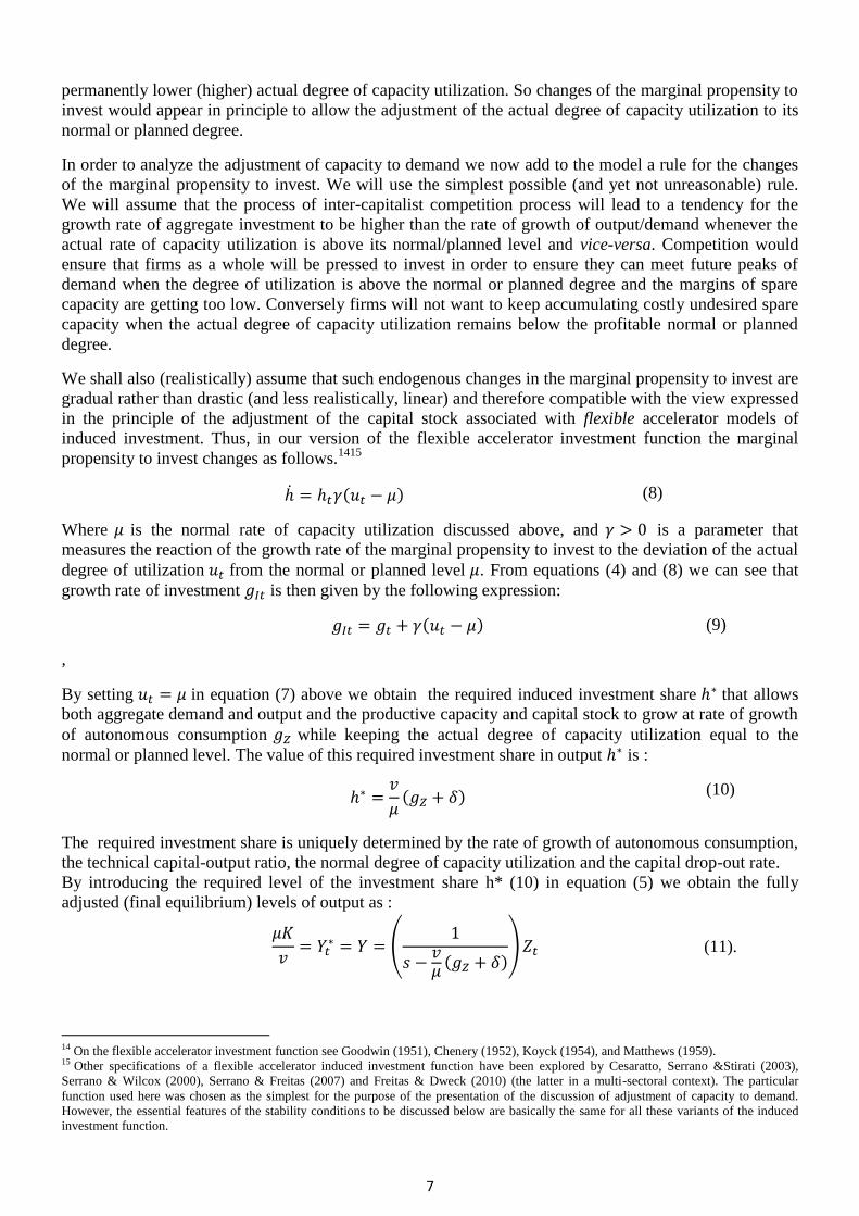
propensity to invest changes as follows.1415

( ) (8)

Where is the normal rate of capacity utilization discussed above, and is a parameter that

measures the reaction of the growth rate of the marginal propensity to invest to the deviation of the actual

degree of utilization from the normal or planned level . From equations (4) and (8) we can see that

growth rate of investment is then given by the following expression:

( ) (9)

,

By setting in equation (7) above we obtain the required induced investment share that allows

both aggregate demand and output and the productive capacity and capital stock to grow at rate of growth

of autonomous consumption while keeping the actual degree of capacity utilization equal to the

normal or planned level. The value of this required investment share in output is :

( )

(10)

The required investment share is uniquely determined by the rate of growth of autonomous consumption,

the technical capital-output ratio, the normal degree of capacity utilization and the capital drop-out rate.

By introducing the required level of the investment share h* (10) in equation (5) we obtain the fully

adjusted (final equilibrium) levels of output as :

(

( )

) (11).

14 On the flexible accelerator investment function see Goodwin (1951), Chenery (1952), Koyck (1954), and Matthews (1959). 15 Other specifications of a flexible accelerator induced investment function have been explored by Cesaratto, Serrano &Stirati (2003),

Serrano & Wilcox (2000), Serrano & Freitas (2007) and Freitas & Dweck (2010) (the latter in a multi-sectoral context). The particular

function used here was chosen as the simplest for the purpose of the presentation of the discussion of adjustment of capacity to demand.

However, the essential features of the stability conditions to be discussed below are basically the same for all these variants of the induced

investment function.

8

Equation (11) shows that at each moment the level of autonomous consumption at and the fully

adjusted (final equilibrium) level of the supermultiplier (the term in parenthesis) determine the levels of

output of the fully adjusted positions (final equilibrium) towards which the economy is slowly

gravitating. In these positions not only aggregate output but also the levels of capacity output and the

capital stock adjust to the levels of aggregate demand.

Note that there are two key conditions for this process of adjustment of capacity to the trend of demand to

work. First, a necessary condition for the adjustment of capacity to demand is the existence of an

exogenous autonomous component of demand that does not create capacity (autonomous consumption in

our case). It is the existence of such expenditures that allows investors to change the investment share

when the levels of investment change. The the existence of autonomous consumption prevents aggregate

demand from always changing in the exact proportion the level of investment has changed. So a

necessary condition for the adjustment of capacity to demand is that the marginal propensity to invest can

be changed by the behavior of investors and this is guaranteed by the existence of autonomous

consumption (and thus of the fraction).

Given our investment function (from equation (5) and (8)) we can obtain the following equation for the

growth rates of aggregate output and demand :

( )

(12).16

Equation (12) shows us that, when the actual and normal degrees of capacity utilization are different, the

rate of growth of output and demand is determined by the rate of expansion of autonomous consumption

plus the rate of change of the supermultiplier given by the second term on the RHS of the above equation.

Hence, if the actual degree of capacity utilization is above (below) the normal/planned degree, capitalist

competition would induce an increase (decrease) in the marginal propensity to invest and, therefore, of

the investment share of output

Changes in the investment share of output, however, both require and cause corresponding and

appropriate modifications in the average saving ratio. But as we mentioned above this endogeneity of the

saving ratio in the model is a consequence of the hypothesis of the existence of positive level of

autonomous consumption. Actually, the latter makes it possible for the fraction ⁄ to change its

value according to the modifications of the investment share of output. As a result, ⁄ ( ) , the ratio of autonomous consumption to aggregate output can change, making the saving ratio an

endogenous variable and allowing its adjustment to the investment share of output. In fact, in the

equilibrium path of the model, once the investment share is determined we can obtain the equilibrium

values of the fraction, of the aggregate autonomous consumption to output ratio and, accordingly, of the

equilibrium value of the saving ratio (i.e., the average propensity to save) as follows

( )

(13)

⁄ ( )

( ) (14)

and

16 The equation is deduced as follows. Taking the time derivatives of the endogenous variables involved in expression

and dividing both sides of the resulting equation by the level of aggregate output, lead us to equation ( ⁄ ) . If

⁄ , then we can solve the last equation for the rate of growth of aggregate output and demand, obtaining

( )⁄ . Finally, we can substitute the right hand side (RHS) of equation (10) in the second term on the RHS of the last equation, which

gives us equation (11) in the text.

9

( )

( ) (15).

We saw that the equilibrium investment share of output is positively related to the equilibrium output

growth rate. Thus, given income distribution (and, therefore, the marginal propensity to save), according

to equations (13), (14) and (15), a higher (lower) equilibrium rate of economic growth entails, on the one

hand, higher (lower) equilibrium values of the fraction and of the saving ratio, and, on the other, a lower

(higher) equilibrium value of the autonomous consumption to output ratio.

While this variability of the investment share in reaction to deviations from the normal degree of capacity

utilization is a necessary for capacity to adjust to demand, it may not be sufficient. For we must also

assume , that the economy remains in a demand led regime throughout the adjustment process, as the

marginal propensity to invest is changing in response to the deviation between actual and planned degree

of capacity utilization. But this, as we have seen (equation(5) above), requires that the marginal

propensity to invest remains lower than the marginal propensity to save. It is possible, if the increase of

the marginal propensity to invest when the degree of capacity utilization is above normal is too big, that

the marginal propensity to investment becomes bigger than the marginal propensity to save, which will

mean a marginal propensity to spend greater than one that obviously implies that induced demand is

being generated at a such high rate that is simply impossible for the supply of output to adjust to it.

Aggregate demand would tend to infinity and there is no change in investment that could adapt capacity

to infinite demand. That is why we have mentioned a gradual change in the marginal propensity to invest

as a response to deviations of capacity utilization from its planned degree. If changes in the marginal

propensity to invest are gradual as to keep the marginal propensity to invest lower than the marginal

propensity to save, this gradual adjustment of the marginal propensity to invest is then the sufficient

condition for the process of adjustment of capacity to demand described above to work.17

In terms of saving, what is happening is that, due to the presence of autonomous consumption, changes in

the marginal propensity to invest are changing the average propensity to save ⁄ by changing the

fraction, the ratio between the average and the marginal propensity to save ⁄ . But the fraction has

to be lower than 1, so changes in the marginal propensity to invest should not be too strong. Thus, as we

shall see with more precision further below there is a close connection between the conditions for the

dynamic stability of the adjustment of capacity to demand and the limits of a demand led growth regime.

In fact since the required induced investment share depends positively on the rate of growth of the

economy, the economy can only be characterized as demand led if the investment share required by the

trend rate of growth plus the extra share of induced investment that occurs as reactions to situations of

deviations of the degree of utilization from the normal planned degree remains below the marginal

propensity to save. This implies that there is a precisely definable maximum rate of growth of

autonomous consumption demand that is compatible with a demand led growth pattern in which capacity

tends to adjust to demand.

IV. Sufficient conditions for the local dynamic stability of the sraffian supermultiplier

In order to arrive at the precise critical value of the marginal propensity to spend that ensures the stability

of the adjustment towards the fully adjusted position and at the same time gives us the exact value of the

maximum rate of demand led growth we must find a set of sufficient conditions for the local dynamic

stability of the model.

17 In Serrano(1995, 1996) the (in itself harmless) auxiliary simplifying assumption that firms correctly foresee the trend rate of growth of

demand as the rate of growth of autonomous demand unfortunately led to the further incorrect argument that any unbiased learning

adjustment process of demand expectations could ensure that capacity could adjust to demand. This is not true if the adjustment of the

investment share is too intense, independently of how demand expectations are formed, the marginal propensity to investment can increase

too fast and endanger the stability of the process. Thus Allain (2013) and Lavoie(2013) are correct in their criticism of this aspect of

Serrano(1995,1996). In Cesaratto, Serrano & Stirati(2003) the correct hypothesis of sufficiently gradual adjustment of the marginal

propensity to invest was made. See the discussion in section VI below.

10

With that purpose in mind let us now substitute equations (12) and (2) into equation (3). Then we obtain a

system of two first order nonlinear differential equations in two variables, the share of investment and

the actual degree of capacity utilization , which we present below:

( ) (8)

( ( )

( ) ) (16)

This is the system that we will use to develop the analysis of the dynamic stability of our sraffian

supermultiplier growth model.

The model is in a fully adjusted position when . Imposing this condition on the system

comprised by equations (8) and (16) yields a system of equations whose solutions are the fully adjusted

values of the degree of capacity utilization and of the investment share of output. From a purely

mathematical point of view the referred system admits two solutions and, therefore, the model has in

principle two possible final equilibrium points, although only one of which has an economic meaning

with strictly positive values for the investment share and the degree of capacity utilization in final

equilibrium. 18

In the latter case from equation (8), if and , then we obtain and the fully

adjusted level of output described by equation (11) above. In terms of growth rates, replacing the final

equilibrium condition in equations (12) and (9) we obtain that the final equilibrium value of the

growth rates of aggregate output (and aggregate demand) and aggregate investment follow the rate of

growth of autonomous consumption . And also, if and , then from equation

(3) we have that and, therefore, as , we also have that:

and thus the

rate of capital accumulation is also driven by the autonomous consumption growth rate.

Let us now look at the stability of this sequence of fully adjusted positions to see if the long period

positions of the economy tend to move towards them. More specifically, we will now analyze the

dynamic stability conditions of the linearized version of the model in the neighborhood of the equilibrium

point (i.e., a local dynamic stability analysis).19

Thus, from the system defined by equations (8) and (16)

we can obtain the corresponding Jacobian matrix evaluated at the equilibrium point with and

( )

[ [

]

[

]

[

]

[

] ]

[

( )

( )

]

The mathematical literature (e.g., for a reference see Gandolfo (1997)) establishes that the necessary and

sufficient stability conditions for a 2x2 system of differential equations are the following:

18 The other equilibrium occurs when the investment share of output and the degree of capacity utilization are both equal to zero (i.e.

). This specific equilibrium, nevertheless, is of no interest, because it represents a completely unrealistic situation from the

economic point of view. However, if such equilibrium were stable, then at least it would reveal that the model had been somehow poorly

specified. But this is not the case, for we can show that the equilibrium in question exhibits an unstable behavior of the saddlepoint type. In

this respect we refer the reader to the more formal treatment of the sraffian supermultiplier model found in Freitas (2014). 19 The legitimacy of an analysis of the local behavior of the nonlinear system using a linearized version of it in the neighborhood of the

equilibrium is discussed in Gandolfo (1997, chap. 21, pp. 361-3). In Freitas (2014) it is shown that the linearized version of the sraffian

supermultiplier model here discussed can be legitimately used to study the dynamic behavior of the model in the neighborhood of its

equilibrium point.

11

[ ]

( )

(17)

and

[ ] ( ) (18).20

The determinant is necessarily positive since we suppose that . Hence, the local stability of

the system depends completely on the sign of the trace of the Jacobian matrix evaluated at the equilibrium

point. Recalling that , inequality (17) implies the following stability condition

( ) (19).

We can interpret (19) as an expanded marginal propensity to spend that besides the final equilibrium

propensity to spend (

( )) includes also a term (i.e., ) related to the behavior of induced

investment outside the fully adjusted position. The extra adjustment term captures the fact that the

investment function of the model is inspired in the capital stock adjustment principle ( a type of flexible

accelerator investment function) and that outside the fully adjusted trend path there must be room not

only for the induced gross investment necessary for the economy to grow at its final equilibrium rate ,

but also for the extra induced investment responsible for adjusting capacity to demand. Thus, ceteris

paribus, for a sufficiently low value of the reaction parameter the system described above is stable.

From the stability condition we can also derive a condition concerning the viability of a demand-led

growth regime for given levels of income distribution and technical conditions of production. Since we

know that ( ⁄ )( ), we can put (19) in the following form:

(20).

This means that, given and , in order for a demand led growth regime to be viable, its equilibrium

growth rate must be smaller than an maximum growth rate given by ( ⁄ ) minus an extra term (i.e., ) associated with the disequilibrium induced investment required for the adjustment of capacity to

demand. This maximum growth rate defines a ceiling for the expansion rate of autonomous demand

compatible with a dynamically stable demand-led growth trajectory according to the supermultiplier

growth model. As can be verified, the ceiling in question, is lower (higher), ceteris paribus, the more

(less) sensitive investment is to changes in the actual rate of capacity utilization (i.e. the higher (lower) is

the reaction parameter ). .21

20 Note that in the general case of a n x n system the stability conditions involving the signs of the trace and determinant of the Jacobian

matrix are only necessary conditions (Gandolfo, 1997, chap. 18, p. 254). The combination of the stated conditions is only sufficient for

stability in the case of a 2 x 2 system. See Ferguson & Lim, (1998, pp. 83-4) for this letter result. Moreover, it can be shown that in the case

envisaged here the equilibrium point is locally asymptotically stable (see, Freitas (2014)). 21 In Serrano (1996) this maximum rate of demand led capacity growth is postulated to be given by the condition

that the

required trend marginal propensity to invest should be lower than the marginal propensity to save. This maximum rate of growth however

may be too high because it does not take into account the extra component of the marginal propensity to invest that occurs during the

disequilibrium adjustment of capacity to demand, which will imply a lower maximum rate of growth. On the other hand, the stability

analysis discussed is this paper only provides sufficient but not necessary conditions for stability. In particular we are assuming both a linear

adjustment of the marginal propensity to invest and that none of the models parameters (in particular the marginal propensity to save and the

technical capital-output coefficient) changes during the cycle. If these assumptions are modified it is easy to build nonlinear examples in

which the economy can remain demand led even if the marginal propensity to invest is bigger than the marginal propensity to save in the

vicinity of the fully adjusted position but cease to be so when actual capacity utilization is sufficiently far from the normal or planned degree.

In any case, the higher maximum rate found in Serrano(1996) is a structural and necessary condition for a demand led growth regime as it

requires that the required investment share/trend marginal propensity to invest should remain below the marginal propensity to save at the

normal degree of utilization and cannot be relaxed.

12

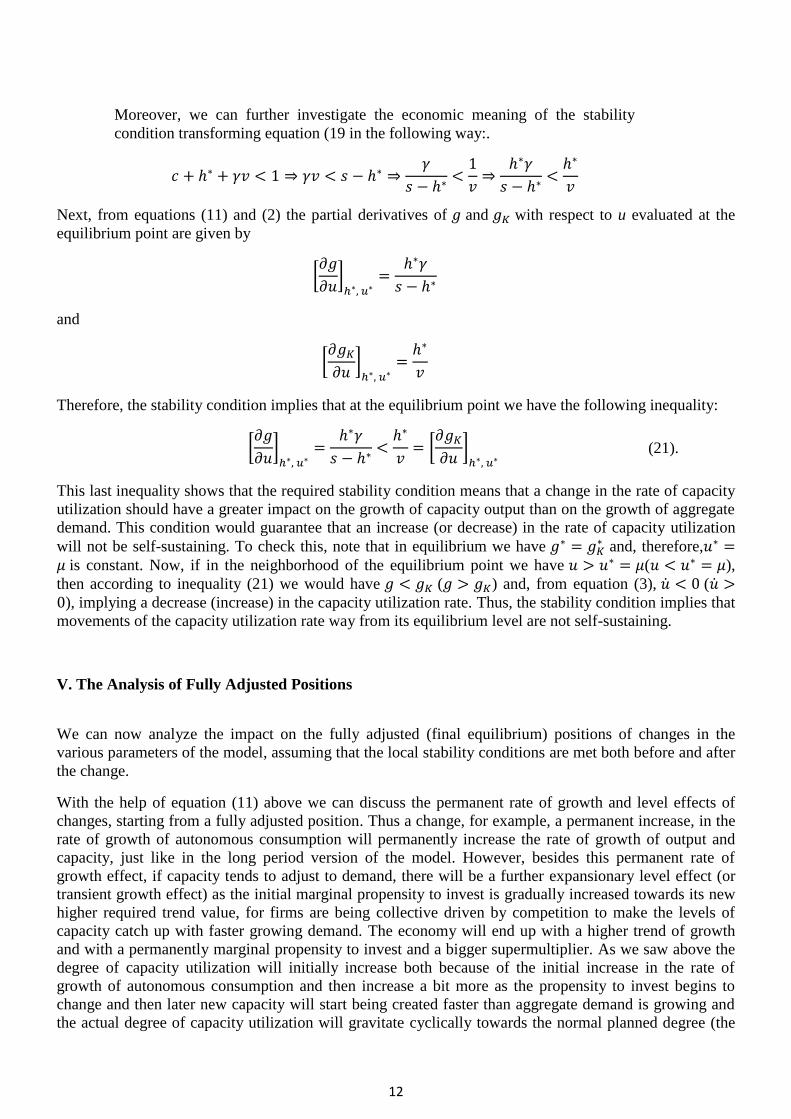
Moreover, we can further investigate the economic meaning of the stability

condition transforming equation (19 in the following way:.

Next, from equations (11) and (2) the partial derivatives of and with respect to u evaluated at the

equilibrium point are given by

[

]

and

[ ]

Therefore, the stability condition implies that at the equilibrium point we have the following inequality:

[

]

[ ]

(21).

This last inequality shows that the required stability condition means that a change in the rate of capacity

utilization should have a greater impact on the growth of capacity output than on the growth of aggregate

demand. This condition would guarantee that an increase (or decrease) in the rate of capacity utilization

will not be self-sustaining. To check this, note that in equilibrium we have and, therefore,

is constant. Now, if in the neighborhood of the equilibrium point we have ( ),

then according to inequality (21) we would have ( ) and, from equation (3), ( ), implying a decrease (increase) in the capacity utilization rate. Thus, the stability condition implies that

movements of the capacity utilization rate way from its equilibrium level are not self-sustaining.

V. The Analysis of Fully Adjusted Positions

We can now analyze the impact on the fully adjusted (final equilibrium) positions of changes in the

various parameters of the model, assuming that the local stability conditions are met both before and after

the change.

With the help of equation (11) above we can discuss the permanent rate of growth and level effects of

changes, starting from a fully adjusted position. Thus a change, for example, a permanent increase, in the

rate of growth of autonomous consumption will permanently increase the rate of growth of output and

capacity, just like in the long period version of the model. However, besides this permanent rate of

growth effect, if capacity tends to adjust to demand, there will be a further expansionary level effect (or

transient growth effect) as the initial marginal propensity to invest is gradually increased towards its new

higher required trend value, for firms are being collective driven by competition to make the levels of

capacity catch up with faster growing demand. The economy will end up with a higher trend of growth

and with a permanently marginal propensity to invest and a bigger supermultiplier. As we saw above the

degree of capacity utilization will initially increase both because of the initial increase in the rate of

growth of autonomous consumption and then increase a bit more as the propensity to invest begins to

change and then later new capacity will start being created faster than aggregate demand is growing and

the actual degree of capacity utilization will gravitate cyclically towards the normal planned degree (the

13

exact symmetric opposite process would happen if the rate of growth of autonomous consumption

decreases).

On the other hand, a permanent change in the marginal propensity to consume (or save) will have a level

effect on output and capacity but no permanent effect on the trend rate of growth. If the marginal

propensity to save decreases (say, because of an exogenous increase in the wage share), initially

consumption and aggregate demand will initially grow faster as the multiplier of the economy has now

increased. But this will be just a level effect as the economy will return to grow at the rate of growth of

autonomous consumption with a higher multiplier and the same required trend investment share. But the

transitory acceleration of growth will lead initially also to an increase in the actual degree of capacity

utilization. And this higher than planned degree of utilization will cause an increase in the marginal

propensity to invest which will itself further expand demand and output and generate more induced

consumption. But over time the new capacity being create by the higher induced investments will grow

faster than aggregate demand and the actual degree of capacity utilization will start falling back cyclically

towards the normal or planned degree and the marginal propensity to invest will tend to stabilize around

its previous required level given by the unchanged rate of growth of autonomous consumption.

Although the marginal propensity to invest as a whole is obviously endogenous in the analysis of the

tendency towards fully adjusted positions (final equilibria) we can still discuss the permanent effects of

changes in its exogenous parameters. Thus, a once for all increase in the technical capital output ratio v,

or in the drop-out rate , as well as a decrease in the planned degree of capacity utilization will all have

a permanent level effect of increasing the required marginal propensity to invest22

(for any given growth

rate of demand ) but will not affect permanently the rate of growth of the economy.23

Growth will

accelerate when these parameters change and have their transitory effects on induced investment as the

actual degree of capacity utilization increases (and this extra induced investment itself generates more

induced consumption). But the marginal propensity to invest and the actual degree of capacity utilization

will keep oscillating cyclically towards the new permanently higher investment share that is required to

allow the level and rate of growth of capacity to adjust to demand at the same unchanged trend rate but

with a bigger supermultiplier.24

The above analysis shows that the main results of the version of the model that makes the

economy gravitate towards fully adjusted (final equilibrium) positions with the actual degree of utilization

tending towards the normal or planned degree are not identical but are in general quite similar and

generally point to the same direction as the results of the long period (medium run) version of the model

in which, because of the exogenously given investment share only the rate of growth of capacity has

adjusted to the rate of growth of demand and the level of capacity may be different from the level of

demand and the actual degree of capacity utilization is different than the normal.

VI. The Sraffian supermultiplier and the warranted rate

VI.1 The warranted rate with growing autonomous consumption After presenting our own results it is standard practice to discuss the relevant literature on the problem. In

the case of the question of the adjustment of capacity to demand and the sraffian supermultiplier this task

becomes quite complex because we consider that the model has been drastically misinterpreted by part of

22 The opposite will happen if all these variables decrease and the normal degree of utilization increases. 23 These changes will, of course, all reduce the maximum rate of growth of the economy. 24 A change or in the sensitivity of the investment share to the discrepancies between actual and normal utilization , starting from a fully

adjusted position with normal utilization prevailing would have no effect on the economy as the investment share would remain unchanged

(apart, of course, of its effect on the maximum rate of growth). If however the economy is not already in the fully adjusted position as it is

bound to be the case , an increased will make investment change more as a reaction to any under or overutilization and this extra

investment itself will have its own multiplier effect on induced consumption. This will certainly affect the cyclical oscillations of the

economy but these will not directly affect either the trend rate of growth of the economy (if the rate of growth of autonomous consumption is

given) nor the trend marginal propensity to invest and the supermultiplier. Thus, in the terms we are using in our discussion changes in will

have a level effect but even this level effect will be temporary as opposed to permanent ( as is instead the case with changes in the other

parameters of the marginal propensity to invest).

14

the literature and presumed mathematical (in)stability proofs have been presented on the basis of the

misinterpreted version of the model. Indeed, although the sraffian supermultiplier is a quite simple model

(being just a multiplier accelerator model fully consistent with a growth trend) some of its critics, for a

number of different reasons, appear to have confused a proposed autonomous consumption demand led

growth model with its exact opposite: the analysis of the effect of autonomous consumption on the rate of

growth of a capacity saving led (supply led) growth model in which Say´s Law hold, which has in

common with it only the presence of an autonomous consumption component that grows.

Many decades ago a number of authors have discussed the impact of autonomous consumption on the so

called harrodian warranted rate, the rate of growth which the economy would follow if starting from a

given initial position of normal capacity utilization the current and future levels of capacity saving

determined the current and future path investment. As it is well known, in a context in which all

consumption is induced by income the warranted rate of growth will be equal to the ratio between the

(net) marginal propensity to save s (in this section for ease of comparison with the literature we will

assume that the drop out ratio is zero and thus s is the net instead of gross marginal propensity to save)

and the normal capital-output ratio (in this section again for ease of comparison we will take the normal

degree of capacity utilization as equal to 1). It is quite obvious that the presence of autonomous

consumption will change this result as autonomous expenditures are a source of (net) dissaving and the

current level of autonomous expenditures reduces capacity saving and thus the ratio of autonomous

expenditures to capacity output (divided by the normal capital-output ratio) will reduce the warranted

rate of growth of the economy of each period compared with what would happen if all consumption was

induced (see Hamberg & Schultze (1961)) and Harrod (1939, 1948)). It is also not difficult to see that if

autonomous consumption grows over time at an independent rate the harrodian warranted rate will in

general not be constant over time since the induced capacity savings will grow at the rate ⁄ while the

autonomous dissaving will grow at a rate that will depend on the rate of growth of autonomous

expenditures.

This warranted rate of growth , the rate of expansion of aggregate demand that would ensure that demand

always adjusts itself fully to capacity (the exact opposite of what we have done so far in this paper) can be

calculated as:

( ⁄ )

(22).

The existence of an autonomous component growing at an independent growth rate of course implies that

such warranted rate growth would, in general, change through time.25

In fact starting from any positive

initial warranted rate we have three possibilities. The first is that, by pure chance, the initial value of

the warranted rate happens to be equal to the rate of growth of autonomous consumption

( ⁄ )

(23).

In this case the share of autonomous consumption in capacity output and thus the share of autonomous

capacity dissaving will remain constant over time which will imply that the average propensity to save at

25 The dynamic behavior of the warranted growth rate incorporating the autonomous consumption component can be expressed by the

following differential equation

( )

( ) (

)

As can be seen from the equation above, the model has two stationary points, and

( ⁄ ).

15

capacity will also be constant and this will determine a constant investment share over capacity output

and a constant rate of growth of capacity output. This is the case in which the warranted rate remains the

same over time. Note that even assuming Say´s law there is absolutely no reason why this should happen

since is determined exogenously.

A second possibility is that the growth rate of autonomous consumption is higher than ⁄ . In this case

the fast growing autonomous dissaving will increase the share of autonomous consumption on capacity

output reducing the capacity savings ratio and the warranted rate of growth of capacity output which will

quickly fall to zero and continue falling as net saving and investment turn negative.

A third logical possibility is that the growth rate of autonomous consumption is lower than ⁄ . In this

case, it is the induced capacity saving that grows at a faster rate and the share of autonomous consumption

and dissaving in capacity output falls through time and the warranted rate of growth will increase over

time until it asymptotically tends to ⁄ as the share of autonomous consumption on capacity becomes

negligible.

VI.2 The stability of the supply determined warranted rate

Surprisingly, the above results about the time path of the savings led warranted rate of growth under

Say´s law became the analytical basis for some of the criticism of the sraffian supermultiplier that have

appeared in the literature.

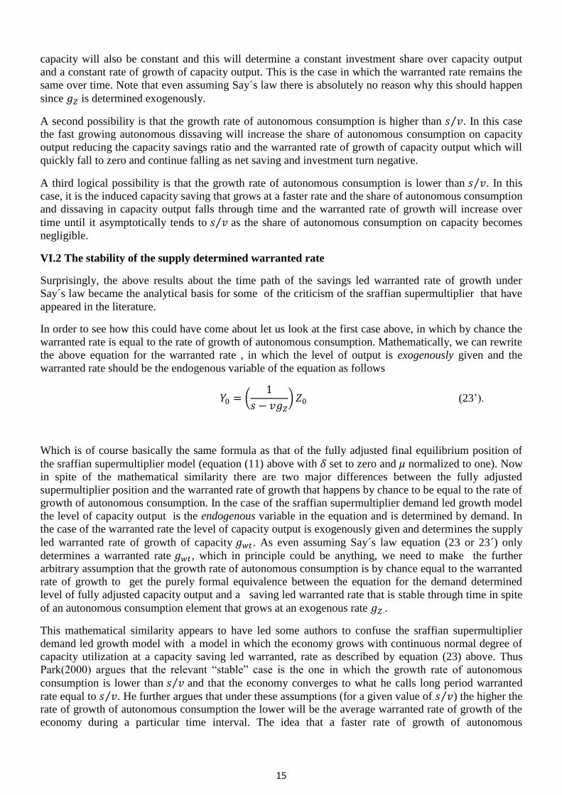
In order to see how this could have come about let us look at the first case above, in which by chance the

warranted rate is equal to the rate of growth of autonomous consumption. Mathematically, we can rewrite

the above equation for the warranted rate , in which the level of output is exogenously given and the

warranted rate should be the endogenous variable of the equation as follows

(

) (23’).

Which is of course basically the same formula as that of the fully adjusted final equilibrium position of

the sraffian supermultiplier model (equation (11) above with set to zero and normalized to one). Now

in spite of the mathematical similarity there are two major differences between the fully adjusted

supermultiplier position and the warranted rate of growth that happens by chance to be equal to the rate of

growth of autonomous consumption. In the case of the sraffian supermultiplier demand led growth model

the level of capacity output is the endogenous variable in the equation and is determined by demand. In

the case of the warranted rate the level of capacity output is exogenously given and determines the supply

led warranted rate of growth of capacity . As even assuming Say´s law equation (23 or 23´) only

determines a warranted rate , which in principle could be anything, we need to make the further

arbitrary assumption that the growth rate of autonomous consumption is by chance equal to the warranted

rate of growth to get the purely formal equivalence between the equation for the demand determined

level of fully adjusted capacity output and a saving led warranted rate that is stable through time in spite

of an autonomous consumption element that grows at an exogenous rate ..

This mathematical similarity appears to have led some authors to confuse the sraffian supermultiplier

demand led growth model with a model in which the economy grows with continuous normal degree of

capacity utilization at a capacity saving led warranted, rate as described by equation (23) above. Thus

Park(2000) argues that the relevant “stable” case is the one in which the growth rate of autonomous

consumption is lower than ⁄ and that the economy converges to what he calls long period warranted

rate equal to ⁄ . He further argues that under these assumptions (for a given value of ⁄ ) the higher the

rate of growth of autonomous consumption the lower will be the average warranted rate of growth of the

economy during a particular time interval. The idea that a faster rate of growth of autonomous

16

consumption will result in lower growth of output and capacity which is understandable under Say´s law

if capacity saving determines investment as autonomous consumption is a source of dissaving. This result

is hardly relevant since there is no reason to think Say´s law has any relevance. Moreover, it is exactly the

opposite of what happens in the sraffian supermultiplier demand led model in which increases in the rate

of growth of autonomous consumption increase the rate of growth of output and productive capacity.26

Schefold (2000) and Barbosa-Filho (2000) have both independently also argued, by seeing the presence

of the required investment share in the fully adjusted position, that the sraffian supermultiplier is based on

a rigid accelerator induced investment function. And both have also claimed that the sraffian

supermultiplier is inherently dynamically unstable. Although it is not true that the model requires the use

of a rigid accelerator (see more on that further below) it is nevertheless true that a rigid accelerator

investment function often is the cause of dynamic instability. The key feature of the rigid accelerator is

the attempt to adjust capacity to demand at once and this tends to make the marginal propensity to invest

very high (in many models equal to the normal capital-output ratio). Since it is reasonable to assume that

empirically the value of the normal capital-output ratio is above one , this may easily lead to a very high

marginal propensity to spend in the vicinity of the normal utilization position and thus (by making the

marginal propensity to spend greater than one) to dynamic instability.

In spite of these references to the rigid accelerator, this was not the route actually taken by Schefold

(2000) and Barbosa-Filho (2000) to demonstrate dynamic instability of the sraffian supermultiplier. They

instead misinterpreted the equivalent of equation (11) for determining the level of output and capacity in

the fully adjusted position of the model as the equivalent of equation (23) that determines the capacity

savings determined supply-led warranted rate of growth. And by doing that what they claim to be the

dynamic instability analysis of the demand led sraffian supermultiplier model with a rigid accelerator is in

fact just a discussion about the path of the warranted rate over time.27

By doing this they naturally find (as

we have seen above) that the warranted rate can only be constant over time if the warranted rate happens

by chance to be equal to the growth rate of autonomous consumption. Since in the sraffian supermultiplier

the rate of growth of autonomous consumption is lower than ⁄ , they see that the warranted rate of

growth will grow over time and asymptotically tend to ⁄ . And then they both then conclude that the

sraffian supermultiplier with a “rigid accelerator” (sic) is dynamically unstable. By confusing a demand

led with a supply led model Schefold (2000)28

and Barbosa-Filho (2000)29

failed to see two basic things.

First, that the proper dynamic stability condition of the disequilibrium adjustment process of a demand

led model as the sraffian supermultiplier depends on the marginal propensity to spend in the vicinity of

the final equilibrium position being lower than one and thus depends on the exact values of the

parameters (as even a demand led model with a rigid accelerator may turn out to be stable).30

They also

failed to see that the totally different question of the time constancy or not of the capacity saving

determined warranted rate is largely irrelevant in a demand led context since generally nothing grows at

the warranted rate and the latter also does not exert any influence on the dynamic behavior of model.

26 Park(2000) confusingly presents his results showing that the growth of autonomous consumption tend to reduce the long period growth of

the economy not as a critique but as “a positive development” of the sraffian supermultiplier model. 27 Barbosa-Filho (2000) bases his analysis on the claim that the sraffian supermultiplier is based on a rigid accelerator investment function.

But a capacity savings led growth model evidently does not have any independent investment function at all. If say´s law holds, the

expression ( ⁄ ) does not contain an investment function at all. The capacity saving ratio on the left hand side determines the

investment share and the warranted rate of growth in the right hand side. Schefold (2000) makes the same mistake. After correctly raising

doubts that a rigid accelerator model would be dynamically stable and even mentioning his own views on the (very high) value of empirical

normal capital-output ratios he suddenly switches to a formal analysis of the path over time of the capacity savings led warranted rate. 28 Schefold (2000, p. 345) refers to the solution for the above differential equation that can be found in Allen (1968, p. 343). In this

connection, it is interesting to note that Allen calls the model under discussion “Equilibrium accelerator-multiplier model”. This designation

refers to the fact that the equation deals only with the determination of the path of the warranted rate over time. In fact, a few pages later

Allen (1968, p. 346) makes use of a “disequilibrium accelerator-multiplier model”, with a lagged accelerator investment function, in order to

deal with the proper issue of the stability of the adjustment of capacity to demand in a situation in which output is determined by demand,

which is the one that would be relevant for the sraffian supermultiplier. 29 Barbosa-Filho(2000, p. 31), uses a nonlinear first order differential equation of the Riccati type that is essentially the same as the one we

used above to discuss the behavior of the warranted rate. In our notation, he analyzes the behavior of the warranted rate according to the

equation ( )(( ⁄ ) ) ( ( ⁄ )) ( ⁄ ) .

30 In fact the correctly formulated stability of this model set in net terms with a rigid accelerator would be vgz+vx<s.

17

Moreover, if the adjustment of capacity to demand in the model happens to be dynamically stable, it is the

warranted rate adjusts itself endogenously to the rate of growth of autonomous consumption as the

marginal propensity to invest tends to the required investment share.

VII. Final Remarks

In this paper we have analyzed the main results of the sraffian supermultiplier model concerning the

crucial role of the rate of growth of the component of autonomous demand that does not generate capacity

for the private sector in determining the trend rate of demand led growth and the purely level effect of

changes in the marginal propensity to consume (or save) and of the exogenous parameters of the marginal

propensity to invest both in the long period equilibrium version of the model in which the actual degree of

capacity utilization may differ persistently from the planned/normal degree and in the complete fully

adjusted equilibrium the actual degree of capacity utilization to gravitates cyclically towards the

planned/normal degree. We also provided a formal analysis and discussed the exact economic meaning (a

marginal propensity to spend lower than one in the neighborhood of the position with normal utilization)

and the relevant implications in terms of the limits for demand led growth (the maximum rate of growth).

Moreover, we have also showed that some of the critics of the sraffian supermultiplier model have

misunderstood either the purpose (or the actual properties) of the model which is of course to generate

demand led growth and some have erroneously thought to have showed the inherent incompatibility of

the model with the principle of effective demand and/or its intrinsic dynamic instability when they were

in fact looking only at the time path of the warranted rate of growth that would occur instead in a quite

uninteresting supply led (Say´s law) model of growth led by capacity savings with autonomous

consumption. We think that the analysis and results of this paper confirm the usefulness of the sraffian

supermultiplier framework to model economic growth as a demand led process that is fully compatible

with the very strong empirical evidence of both the quite stable average actual degrees of capacity

utilization and the dampened cycles of private investment in machinery and equipment (typical flexible

accelerator processes). To us it is quite encouraging that, starting from a different approach, neo-

kaleckian authors such as Allain (2013) and Lavoie (2013) are reaching similar conclusions. More

theoretical and empirical research is needed in two fronts. We need a richer discussion of the

determinants of the induced changes in the marginal propensity to invest, which was here presented in the

simplest possible terms on purpose just to illustrate how capacity tends to adjust to the trend of effective

demand. More importantly, research efforts should focus on the determinants and dynamics (particularly

financial) of the trend of growth of the different “unproductive” autonomous components of demand.

References

Allain, O. (2013) “Growth, Income Distribution and Autonomous Public Expenditures”, paper presented

at the 1st joint conference AHE - IIPPE - FAPE, Political Economy and the Outlook for Capitalism,

Paris, July 5-7, 2012.

Barbosa-Filho, N. H. (2000) “A Note on the Theory of Demand Led Growth”, Contributions to Political

Economy, vol. 19, pp. 19-32.

Cesaratto, S., Serrano, F. & Stirati, A. (2003) “Technical Change, Effective Demand and Employment”,

Review of Political Economy, vol. 15, n. 1, pp. 33 - 52.

Chenery, H. B.: (1952), “Overcapacity and the acceleration principle”, Econometrica, vol. 20, no. 1, pp.

1–28.

Ciccone, R. (1986)“Accumulation and Capacity Utilization: Some Critical Considerations on Joan

Robinson's Theory of Distribution”, Political Economy. Studies in the Surplus Approach, vol. 2 (1),

pp.17-36.

Ciccone, R. (1987) “Accumulation, Capacity Utilization and Distribution: a Reply”, Political Economy.

Studies in the Surplus Approach, vol. 3 (1), pp. 97-111.

18

Ciccone R (2011) Capacity utilization, mobility of capital and the classical process of gravitation , in ;

Gehrke, Christian & Mongiovi, Gary (orgs.) Sraffa and modern economics; Vol. 2 (London,

Routledge).

Ferguson, B. S. & Lim, G. C. (1998) Introduction to Dynamic Economic Models, (Manchester,

Manchester University Press).

Freitas, F. & Dweck, E. (2010) “Matriz de Absorção de Investimento e Análise de Impactos

Econômicos”, in Kupfer, D., Laplane, M. F. &Hiratuka, C. (Coords.) Perspectivas de Investimento

no Brasil: temas transversais, (Rio de Janeiro, Synergia).

Freitas, F. (2014) “Notes on the Dynamics of the Sraffian Supermultiplier Growth Model”, mimeo, IE-

UFRJ.

Gandolfo, G. (1997) Economic Dynamics, (Heidelberg, Springer-Verlag).

Garegnani, P. (1992) “Some notes for an analysis of accumulation”, in Halevi, J. Laibman, D. & Nell, E.

(eds.) Beyond the Steady State: a Revival of Growth Theory (London, Macmillan).

Garegnani, P. (2014[1962]) “The Problem of Effective Demand in the Italian Economic Development”,

Review of Political Economy, forthcoming.

Goodwin, R. (1951), “The nonlinear accelerator and the persistence of business cycles”, Econometrica,

vol. 19, n. 1, pp. 1–17.

Hamberg, D & Schultze, C. (1961) Autonomous versus induced investment: The interrelatedness of

parameters in growth models, The Economic Journal, vol. 71 (281), pp. 53-65.

Harrod, R. (1939),“An Essay in Dynamic Theory”, The Economic Journal, Vol. 49, No. 193, pp. 14-33.

Harrod, R. (1948),Towards Economic Dynamics: Some Recent Developments of Economic Theory and

their Application to Policy (London, Macmillan)

Koyck, L.: (1954), Distributed lags and Investment Analysis, (Amsterdam, North Holland).

Lavoie, M. (2013) “Convergence towards the normal rate of capacity utilization in Kaleckian models”,

mimeo, University of Ottawa.

López, J & Assous, M. (2010) Michal Kalecki, (London, Palgrave Macmillan).

Palumbo, A. & Trezzini, A. (2003) "Growth without normal capacity utilization," The European Journal

of the History of Economic Thought, vol. 10 (1).

Park, M.-S.(2000), “Autonomous Demand and Warranted Rate of Growth”, Contributions to Political

Economy, vol. 19, pp. 1-18.

Schefold, B. (2000) “Fasidell’accumulazione e mutevoli influenze sulla distribuizione”, in Pivetti, M.

(ed.) PieroSraffa: contributti per una biografiaintellettuale, (Rome, Carocci), 2000.

Serrano, F. (1996) The Sraffian Supermultiplier, Unpublished PhD Thesis, Cambridge University, UK.

Serrano, F. (1995). “Long Period Effective Demand and the Sraffian Supermultiplier”, Contributions to

Political Economy, vol. 14, pp. 67-90.

Serrano, F. & Wilcox, D. (2000). “O modelo de dois hiatos e o supermultiplicador”, Revista de Economia

Contemporânea, vol. 4, n. 2, pp. 37 – 64.

Serrano, F. (2001) “Acumulação e gasto improdutivo na economia do desenvolvimento”, em Fiori, J. L.

& Medeiros, C. A. (orgs.) Polarização mundial e Crescimento, (Petrópolis, Editora Vozes).

Serrano, F. (2007) “Histéresis, Dinámica Inflacionaria y el Supermultiplicador Sraffiano”, In: Serrano, F.

(2007) Seminarios Sraffianos. Buenos Aires: Edicciones Cooperativas, 2007.

Serrano, F.& Freitas, F. (2007) “El Supermultiplicador Sraffiano y el Papel de la Demanda Efectiva em

los Modelos de Crecimiento”. Circus, vol. 1, pp. 19-35