Growth Networks∗

Raja Kali† Javier Reyes‡ Josh McGee§

Stuart Shirrell¶

JEL Classification: F15, O40, F43.

Keywords: trade, growth acceleration, networks, small-world

First Version, October 2009. This version, June 2012.

Abstract

We map the relationship between products in global trade and the products a

country exports as a network to devise a measure of the density of links between

the products in a country’s export basket and a measure of network proximity from a

country’s export basket to products that a country does not export. We use the density

measure as a proxy for synergies between the products in a country’s export basket.

The network proximity measure gives us an indicator of how diffi cult it is likely to be

for a given country to move from its current product specialization to new products.

We find that the density of links within the products constituting a country’s export

basket and the network proximity to new products are of concurrent importance for a

poor country to move to higher income products and experience higher growth rates.

∗We are grateful to Jungmin Lee, Fabio Mendez, Russell Hillberry, Eric Verhoogen (the editor), andanonymous referees for comments which improved the paper. We also thank seminar participants at ANU-Canberra, University of Arkansas, IIFT-Kolkata, the 2009 EITG (Melbourne) and 2010 EIIT (Chicago)conferences for helpful feedback.†HEC Montreal, raja.kali@hec.ca‡University of Arkansas, jreyes@walton.uark.edu§Laura and John Arnold Foundation, joshbmcgee@gmail.com¶University of Arkansas, sshirrell@uark.edu.

1

1 Introduction

Until quite recently, few relationships enjoyed as much consensus among economists as that

between trade and growth. The view that integration into the global economy is a reliable

way for countries to grow permeated advice from multilateral institutions such as the World

Bank, the IMF, the OECD, as well as discussions by distinguished economists (Krueger, 1998;

Fischer, 2000, for example). This view was supported by an influential body of research,

the best known of which are papers by Dollar (1992), Sachs and Warner (1995), Ben-David

(1993), and Frankel and Romer (1999). However, the consensus has been thrown into

disarray by criticism of this literature over problems in measuring openness, the statistical

sensitivity of specifications, the collinearity of protectionist policies with other bad policies,

and other econometric diffi culties (Rodriguez and Rodrik, 2000; Harrison and Hanson, 1999).

This has led to scepticism regarding the existence of a general, unambiguous relationship

between openness and growth. A recent attempt to update the Sachs and Warner approach

by Waczairg and Welch (2008) notes that while the evidence paints a favorable picture of

outward-oriented policy reforms on average, it cautions against one-size-fits-all policy that

disregards local circumstances. Focus has therefore shifted to a scrutiny of the channels

through which trade openness may influence economic performance, and the way in which the

relationship between trade and growth is contingent on country and external characteristics.

We contribute to this literature by identifying a novel mechanism which facilitates tran-

sition to a high growth path. We focus on the relationship between products in global trade

and the characteristics of a country’s pattern of product specialization as revealed through

its exports. The pattern of relatedness among products in global trade is referred to as

“product space”in work by Hausmann and Klinger (2007) and Hidalgo et. al. (2007). It

seems natural to interpret “product space”in terms of a network where products represent

nodes and the linkages between them represent pair-wise relationships among products. We

therefore adopt a network interpretation of product space, which enables us to draw upon

analytical methods from the recent literature on complex networks1. Explicitly mapping

product space as a network and then superimposing a country’s pattern of product special-

ization on product space enables us to devise a measure of the density of links between the

products in a country’s export basket and a measure of how close a country’s product spe-

cialization pattern is to the rest of product space. We use the density measure as a proxy

for synergies between the products in a country’s export basket. The closeness measure

gives us an indicator of how easy it is likely to be for a given country to move from its

1Newman (2000) and Albert and Barabasi (2002) are good overviews of this literature. Jackson (2009)and Goyal (2008) are good introductions to the economics of networks.

2

current product specialization to new products. We suggest that the density of links within

the products constituting a country’s export basket and the closeness to new products are

of concurrent importance for a poor country’s ability to move to new products and higher

growth rates.

One of the general results of the literature on complex networks is that high performance

networks in many settings (biological, technological, social, economic) have the “small-world”

property (Watts and Strogatz, 1998; Watts, 2004; Albert and Barabasi, 2002; Goyal et. al,

2006). A small-world is a network whose topology combines high clustering among nodes

with short average distance (path length) across nodes. Inherent in most networks is a

trade-off between short distance across nodes and high clustering among nodes, since one

comes at the expense of the other if link formation is costly. By balancing this trade-off, the

small-world is considered an “effi cient”topology. Our approach is motivated by the small-

world idea. However, instead of focusing on a structural property of the whole network, we

focus on the characteristics of a country’s product specialization pattern and its position in

the product space network.

In our context, nodes are products, and we associate a high density of links between nodes

in the network with synergies between products. But since we cannot directly measure these

synergies we remain agnostic about a myriad of possible sources, such as complementarity

in technology, information, infrastructure, resources, and public policy. Short average path

length (which we refer to subsequently as network proximity) provides the potential for

leaps across the network, to new products. Both features are advantageous in the context

of economic development and growth. Could it be that the key to acceleration in the rate

of growth is whether the pattern of product specialization of a country (as reflected in its

export basket) develops a propitious intersection of density and network proximity before

the take-off?

Why should such a configuration for a country in product space facilitate a transition in

economic growth? The economic intuition is straightforward. A high density of links be-

tween products enables agglomeration externalities and synergies of various kinds. Network

proximity allows “leaps”across product space to new products. The extent of agglomera-

tion externalities determine cost reductions, freeing up resources for investment. Investment

capabilities in turn determine how far a country can leap. Network proximity determines

how far a country needs to leap to reach new products. The relationship between density of

links between products and network proximity thus plays a role in determining the likelihood

of a leap to a higher growth path. We present a more detailed discussion of this intuition in

section 2. If true, then this implies that a country’s location in product space and its pattern

of product specialization matter for its likelihood of experiencing a growth acceleration. If

3

we can find evidence for this line of reasoning, then we will have made progress in decoding

the mystery of growth acceleration and its relationship to trade and comparative advantage.

Examining this insight is the primary objective of this paper. These arguments are closely

related to the literature on successful industrial districts (such as Silicon Valley as studied

by Saxenian, 1994 and Castilla et. al., 2000) or city growth (Jacobs, 1984; Glaeser et. al.,

1992). However, prior perspectives have not explicitly adopted network methods, which

enable quantification of these patterns.

We use these ideas to explain transitions in economic growth classified by Hausmann,

Pritchett and Rodrik (2005) as “growth accelerations”2. We focus on sharp transitions in

the growth path rather than economic growth per-se because the mechanism we have in

mind pertains to the ability of a country to move to new products and change its production

structure. Such a change should have a discrete effect on economic growth, if it does have

an effect at all3. An increase in the economic growth rate is a long-run effect, a complex

phenomenon to which we do not have much new to add in this paper. Also, focusing on

well defined growth acceleration episodes is advantageous because it circumvents common

problems faced by growth regressions which assume a single model for all countries when

in reality different countries may be at different stages of development, as well as standard

endogeneity concerns associated with growth regressions.

Hausmann et. al. find growth accelerations to be highly unpredictable. The vast

majority of growth accelerations are unrelated to standard determinants such as political

change and economic reform, and most instances of economic reform do not produce growth

accelerations. This leaves us with a conundrum. Are growth accelerations idiosyncratic

and a matter of luck? The implications of such a conclusion would be distressing, to say the

least. But while the mechanics of these transitions continue to be a mystery, the good news

is that Hausmann et. al. find that growth accelerations are a fairly frequent occurrence. Of

the 110 countries in their sample, 60 have had at least one acceleration in the 35-year period

between 1957 and 1992 —a ratio of 55 percent.

A related paper is Hidalgo and Hausmann (2009). Their hypothesis is that the produc-

tivity of a country resides in the diversity of its available nontradable “capabilities,” and

therefore, cross-country differences in income can be explained by differences in economic

complexity, as measured by the diversity of capabilities present in a country and their inter-

actions. They interpret trade data as a bipartite network in which countries are connected

2Growth accelerations are defined as rapid growth episodes that satisfy the following conditions: (i) per-capita income growth increase ≥ 2% per year, (ii) the increase in growth has to be sustained for at least 8years, (iii) the post-acceleration growth has to be at least 3.5% per year, and (iv) post-acceleration outputhas to exceed the pre-episode peak level of income, to rule out cases of pure recovery.

3We explain this in more detail in Section 4.

4

to the products they export, and show that it is possible to quantify the complexity of a

country’s economy by characterizing the structure of this network. Their measures of com-

plexity are correlated with income, and deviations from this relationship are predictive of

future growth. Our paper shares a focus on economic growth and the use of network mea-

sures based on trade data with theirs. However, our growth mechanism, based on synergies

between products and the costs of shifting to new products, is quite different. Our net-

work variables therefore have a different purpose and are consequently different from their

measures. We therefore view our contribution as distinct from and complementary to their

work.

A summary of our methodology and findings is as follows.

1. First, we examine the transformation of product space across time, from 1965 to 2000.

This provides us with evidence that the product space network of relatedness among

products (which we refer to subsequently as the proximity matrix) based on the pattern

of revealed comparative advantage in world trade has evolved considerably over this

period.

2. Second, we map the product specialization pattern (i.e., the export basket, viewed as anetwork of products) of individual countries in our dataset over the period 1965-2000.

Then, for every year, we superimpose country-level product specialization on to the

(global) proximity matrix. Superimposing the country-level product specialization

“sub”-network on to the larger proximity matrix enables us to identify network prop-

erties of country-level product specialization. From this we obtain network measures

of the density of links within a country’s export products and network proximity to po-

tential products. We use these measures to suggest that countries which experienced

episodes of growth acceleration had an overlap between their product specialization

pattern and the proximity matrix which provided a propitious intersection of the den-

sity of links between current products and network proximity to potential new prod-

ucts prior to growth acceleration, while countries which failed to experience subsequent

growth acceleration did not.

3. Third, we run a multivariate probit regression to examine if there is large sample

support for the hypothesis that both density and network proximity are of concurrent

importance in a country’s ability to leap to new products and experience subsequent

growth acceleration. We find that our network measures are statistically significant

in predicting a heightened probability of experiencing subsequent growth acceleration.

4. Fourth, we use the network-based density and network proximity measures computed

5

from our data in conjunction with the estimated coeffi cients from the regression to build

a grid of the probability function for different density-network proximity combinations.

This exercise demonstrates that the shape of the high probability region resembles an

arc. The arc implies that our measure of the density of links between products

and network proximity to new products are related in a non-monotonic fashion for a

heightened probability of experiencing a growth acceleration. We also find that the

probability of growth acceleration falls off quite sharply outside of the arc traced by

this exercise. We explain the intuition behind these findings below.

By bringing a network approach to the proximity matrix and then using these measures

to explain growth acceleration, we bring disparate strands of research together, and, we

hope, provide a distinct and valuable contribution to the literature on trade, comparative

advantage, and economic growth. In the next section we explain our hypothesis and the

network approach in more detail. Section 3 outlines our empirical strategy. Section 4

presents results. Section 5 concludes.

2 Product Space, Country Specialization, and the Hy-

pothesis

Product SpaceWe follow Hidalgo et. al. (2007) and Hausmann and Klinger (2007) in computing the

product space of relatedness among products based on the pattern of revealed comparative

advantage in world trade. We provide a brief description here; the reader is referred to

their papers for more detail. Like them, we use the NBER World Trade Database for the

computation of product space (Feenstra et. al., 2005).

The first step is the computation of “revealed comparative advantage” (RCA), which

measures whether a country c exports more of good i, as a share of its total exports, than

the “average”country (i.e., RCA>1 not RCA<1).

RCAc,i =

exp(c,i)∑i exp(c,i)∑c exp(c,i)∑c,i exp(c,i)

(1)

If RCAc,i > 1, then country c is considered to have “revealed comparative advantage”

in product i. This exercise yields a set of 0/1 variables across all possible products i for

each country c. The RCA set, thus computed for every country in the data, is then used to

6

compute the “proximity”φ between every pair of products i and j,

φi,j = min{P (RCAi|RCAj), P (RCAj|RCAi)} (2)

The proximity φi,j between products i and j is thus the minimum of the pair-wise condi-

tional probabilities of goods being exported together. Note that this is computed from the

“global”data of RCA sets of all countries in the data calculated in the previous step (as in

1), and is a probability function based on the number of countries exporting a good given

that they export another. As Hidalgo et al. (2007) note, proximity (φi,j) “formalizes the

intuitive idea that the ability of a country to produce a product depends on its ability to

produce other related products. If two goods are related because they require similar insti-

tutions, infrastructure, resources, technology, or some combination thereof, they will likely

be produced in tandem, whereas dissimilar goods are less likely to be produced together.”

In other words, if φi,j is high then products i and j are frequently exported together, while

if φi,j is low then they are rarely exported together by the same country.

The matrix of these proximities characterizes product space. We refer to this in the

rest of the paper as the proximity matrix. We compute the proximity matrix for every year

between 1965 and 2000, using data for 187 countries, using trade data at the 4-digit product

level (SITC). These matrices can be compared to understand how product space has evolved

during this period. The proximity matrix can be considered a complex network4, where each

product represents a node in the network and the edges between them and their intensities

are the likelihood of these goods being exported together as measured by φi,j. Given the

symmetry of the proximity matrix, the network resulting from it can be characterized as a

weighted, undirected network. This perspective then allows us to analyze the proximity

matrix and its evolution in terms of the properties of the network. In the rest of the paper

we use the term proximity matrix rather than product space since the former phrase seems

more intuitive in an economics context.

It is worth noting that the proximity measure (φi,j) is distinct from the Ellison and

Glaeser (1997, hereafter EG) metric of coagglomeration. The EG index measures whether

the coagglomeration of industries in geographic space is greater than what would be expected

to arise randomly. The Hidalgo et. al. definition of proximity on the other hand is

indicative of synergies and complementarity between products, which could conceivably lead

to geographic coagglomeration. The EG index thus measures geographic co-location while

4Complex networks are large scale graphs that are composed of so many nodes and links that they cannotbe meaningfully visualized and analyzed using standard graph theory. Recent advances in network researchnow enable us to analyze such graphs in terms of their statistical properties. Albert and Barabasi (2002)and Newman (2003) are good surveys of these methods.

7

proximity measures co-location within countries’export baskets. In a companion paper,

Ellison, Glaeser and Kerr (2010) relate coagglomeration levels to the degree to which industry

pairs share goods, labor, or ideas, and find support for all three of Marshall’s theories of

agglomeration with input-output linkages particularly important. We do not, however,

have the data to identify these spillovers in our study and therefore remain agnostic about

the sources of proximity.

Country Level Product SpecializationThe set of products for which a country possesses RCA (>1) is referred to as country

level product specialization. As described above, this is a Ix1vector of 0/1 variables across

all possible products i for each country c. This is the comparative advantage of a country

as revealed through its exports. We can examine how this set has changed over the time

period of our data for countries which experienced growth acceleration and those that did

not. Essentially, the set of products for which a country has RCA>1 can be considered

as a sub-network of the proximity matrix. In other words, this sub-network is defined by

the products for which a country has revealed comparative advantage with the weighted

link between each pair of products corresponding to the likelihood of them being exported

together (i.e., the relatedness measure φi,j reported in the proximity matrix, which is derived

from the "global" data on RCA sets).

The HypothesisOnce we have obtained a country’s level product specialization set characterized as a sub-

network of the proximity matrix as described above, we can use this to compute a network

measure of the density of links between the products in a country’s product specialization

set. Since higher density is associated with greater relatedness across the products in a

country’s product specialization set, the density measure gives us a proxy for synergies within

a country’s product specialization set. We can also compute a network-based measure of

the closeness between a country’s product specialization set and the rest of the proximity

matrix, i.e., to the products in the proximity matrix that are not in the export basket of a

country. We refer to this measure as network proximity. Since greater network distance to

the rest of product space is associated with more intermediate steps that need to be traversed

to reach other “new”products, the network proximity measure gives us a proxy for the ease

(or the costs) of leaping to new products. Our conjecture is that both density and network

proximity are of concurrent importance in a country’s ability to leap to new products and

experience a transition to higher economic growth.

Making a leap to a new product requires an investment of resources, and co-location

of “nearby”sectors in the proximity matrix yields synergies that help in reducing costs or

freeing up resources to make that investment. The cost of making a leap is increasing

8

in the “distance” that has to be traveled to a new product. Hence there is likely to be

a relationship between density (within a country’s own products) and network proximity

(to new products) in determining the likelihood of a leap to a new product. In order to

develop this reasoning further, it is helpful to consider the trade-offs involved in leaping to

new products in more detail. The intuition can be understood by considering the following

density-network proximity configurations5.

First, consider a situation where a country’s export basket (product specialization set)

is located in a part of the proximity matrix such that both density and network proximity

to new products are low. Then the lack of synergies among the current set of products

can be an obstacle to leaping due to the inability to reduce costs and free up resources to

generate the (distant and thus costly) leap to new products. Low density and low network

proximity can thus impose a “feasibility constraint”on the leap. This implies that if density

is low then network proximity needs to be high in order to ensure leap feasibility. The leap

feasibility constraint thus suggests a negative relationship between network proximity and

density at low levels of density.

Next, consider a situation where a country’s export basket is located in a part of the

proximity matrix such that density is high and network proximity is low. In this case, it

is possible for high synergies create an “inertia effect”by dampening the incentive because

leaping to new products implies forsaking current synergies, especially if synergies around

a potential new product take time to develop, as seems reasonable. High density can thus

create an “incentive constraint”on the leap. This implies that high network proximity is

especially desirable when density is also quite high, in order to surmount the leap incentive

constraint. The leap incentive constraint thus suggests a positive relationship between

density and network proximity at high levels of density.

The leap mechanism thus involves two constraints: a leap feasibility constraint and a

leap incentive constraint. Putting the two constraints together then implies that whether

the relationship between density and network proximity is positive or negative depends on

whether the leap incentive constraint or the leap feasibility constraint is respectively binding.

At low values of density it is likely that the leap feasibility constraint will bind, leading us

to expect a negative relationship between density and network proximity. At high values of

density it is likely that the leap incentive constraint will bind, leading us to expect a positive

relationship between density and network proximity. In sum, this leads us to conjecture

that if we were to superimpose country level product specialization on the proximity matrix,

we would find that a higher likelihood of experiencing growth acceleration is associated with

5The working paper version of the paper outlines a simple algebraic model which develops the intuitionthat follows and is available from the authors.

9

a distinct and non-monotonic relationship between density and network proximity.

To test these implications empirically, we devise network measures of synergies and dis-

tance. We describe these in section 3.3.

3 Empirical Strategy

There are several steps to our empirical strategy. First, we examine the transformation of

product space across time, from 1965 to 2000. This provides us with evidence that the

product space network of relatedness among products (the proximity matrix) based on the

pattern of revealed comparative advantage in world trade has evolved considerably over this

period. Then we present evidence consistent with the idea that countries which subsequently

experienced growth acceleration had an overlap between their product specialization pattern

and the proximity matrix that created propitious conditions with respect to distance and

network proximity as described above.

This provides the motivation for obtaining network measures of the density of links

within a country’s export products and network proximity to potential products. We then

use these measures in a multivariate probit regression to examine if there is large sample

support for the hypothesis that if a country’s pattern of product specialization exhibits a

propitious intersection between the density of links between current products and average

network proximity to potential new products then it is more likely to experience subsequent

growth acceleration.

3.1 The Transformation of Product Space

In order to examine the overlap between the proximity matrix and country-level product

specialization, we first examine the evolution of the connectedness of the proximity matrix

over time. For this purpose we use methods developed in the physics literature to detect

community structure in networks, meaning the existence of some natural division of the

network such that nodes within a group/sub-network are highly associated (i.e. high prox-

imity) among themselves while having relatively fewer/weaker connections with the rest of

the network. In our context, a community of nodes signifies products likely to be exported

together, due to synergy and complementarity of various kinds between them.

The partitioning of a network into communities can be done in different ways. One way

is to use a community structure algorithm that determines the most appropriate community

structure without prior knowledge about the network and is able to distinguish between

networks having clear community structure and networks with essentially random structure.

10

This method is also referred to as hierarchical clustering. This approach organizes the data

into communities based solely on the data. There are no assumptions made regarding the

specific members of each cluster or the number of clusters to be identified. This approach

provides insight into the transformation of product space as a whole.

The community structure (hierarchical clustering) algorithm for networks that we use

here was proposed by Ruan and Zhang (2008) and is referred to as QCUT. This methodology

is a refinement of the algorithm proposed by Newman (2007). We first use the QCUT

algorithm to identify communities into which the product space is partitioned for every year

and then we compare the community structures across years.

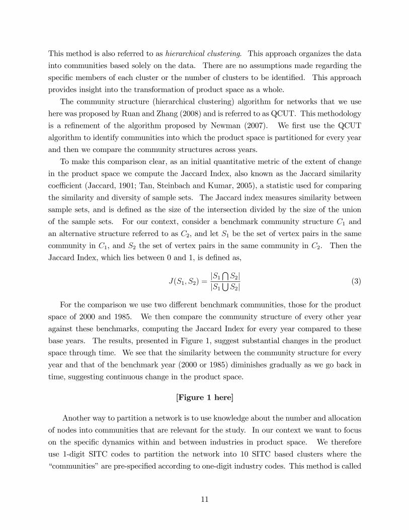
To make this comparison clear, as an initial quantitative metric of the extent of change

in the product space we compute the Jaccard Index, also known as the Jaccard similarity

coeffi cient (Jaccard, 1901; Tan, Steinbach and Kumar, 2005), a statistic used for comparing

the similarity and diversity of sample sets. The Jaccard index measures similarity between

sample sets, and is defined as the size of the intersection divided by the size of the union

of the sample sets. For our context, consider a benchmark community structure C1 and

an alternative structure referred to as C2, and let S1 be the set of vertex pairs in the same

community in C1, and S2 the set of vertex pairs in the same community in C2. Then the

Jaccard Index, which lies between 0 and 1, is defined as,

J(S1, S2) =|S1

⋂S2|

|S1

⋃S2|

(3)

For the comparison we use two different benchmark communities, those for the product

space of 2000 and 1985. We then compare the community structure of every other year

against these benchmarks, computing the Jaccard Index for every year compared to these

base years. The results, presented in Figure 1, suggest substantial changes in the product

space through time. We see that the similarity between the community structure for every

year and that of the benchmark year (2000 or 1985) diminishes gradually as we go back in

time, suggesting continuous change in the product space.

[Figure 1 here]

Another way to partition a network is to use knowledge about the number and allocation

of nodes into communities that are relevant for the study. In our context we want to focus

on the specific dynamics within and between industries in product space. We therefore

use 1-digit SITC codes to partition the network into 10 SITC based clusters where the

“communities”are pre-specified according to one-digit industry codes. This method is called

11

graph partitioning. This approach provides insight into the rise and decline of specific

industries over time in terms of network connectedness.

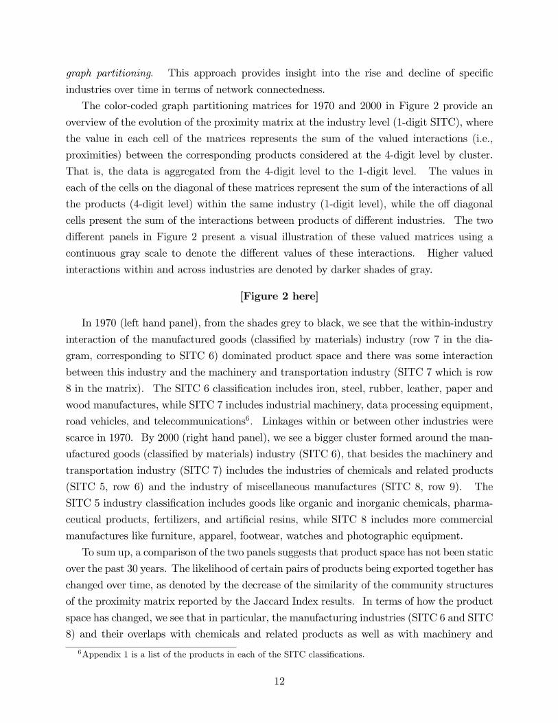
The color-coded graph partitioning matrices for 1970 and 2000 in Figure 2 provide an

overview of the evolution of the proximity matrix at the industry level (1-digit SITC), where

the value in each cell of the matrices represents the sum of the valued interactions (i.e.,

proximities) between the corresponding products considered at the 4-digit level by cluster.

That is, the data is aggregated from the 4-digit level to the 1-digit level. The values in

each of the cells on the diagonal of these matrices represent the sum of the interactions of all

the products (4-digit level) within the same industry (1-digit level), while the off diagonal

cells present the sum of the interactions between products of different industries. The two

different panels in Figure 2 present a visual illustration of these valued matrices using a

continuous gray scale to denote the different values of these interactions. Higher valued

interactions within and across industries are denoted by darker shades of gray.

[Figure 2 here]

In 1970 (left hand panel), from the shades grey to black, we see that the within-industry

interaction of the manufactured goods (classified by materials) industry (row 7 in the dia-

gram, corresponding to SITC 6) dominated product space and there was some interaction

between this industry and the machinery and transportation industry (SITC 7 which is row

8 in the matrix). The SITC 6 classification includes iron, steel, rubber, leather, paper and

wood manufactures, while SITC 7 includes industrial machinery, data processing equipment,

road vehicles, and telecommunications6. Linkages within or between other industries were

scarce in 1970. By 2000 (right hand panel), we see a bigger cluster formed around the man-

ufactured goods (classified by materials) industry (SITC 6), that besides the machinery and

transportation industry (SITC 7) includes the industries of chemicals and related products

(SITC 5, row 6) and the industry of miscellaneous manufactures (SITC 8, row 9). The

SITC 5 industry classification includes goods like organic and inorganic chemicals, pharma-

ceutical products, fertilizers, and artificial resins, while SITC 8 includes more commercial

manufactures like furniture, apparel, footwear, watches and photographic equipment.

To sum up, a comparison of the two panels suggests that product space has not been static

over the past 30 years. The likelihood of certain pairs of products being exported together has

changed over time, as denoted by the decrease of the similarity of the community structures

of the proximity matrix reported by the Jaccard Index results. In terms of how the product

space has changed, we see that in particular, the manufacturing industries (SITC 6 and SITC

8) and their overlaps with chemicals and related products as well as with machinery and

6Appendix 1 is a list of the products in each of the SITC classifications.

12

transportation equipment industry have been the sectors that have experienced the clearest

transformations in terms of becoming more tightly connected to surrounding industries.

3.2 Country-Level Specialization and Overlap with Product Space

Here we combine information from the “global” proximity matrix with “local” country-

level patterns of product specialization by superimposing country-level patterns of product

specialization on to the proximity matrix to see if there is evidence consistent with our

hypothesis. If a country’s product specialization lies in industries that are in the tightly

connected regions of the proximity matrix then it is better positioned to take advantage of

synergies within those industries and also across industries which overlap with the densely

connected set. This overlap of a country’s product specialization with the connected regions

of the proximity matrix enables synergies of various kinds between products, which reduce

production costs and free up resources for investment. Second, if the average network

proximity to new products is low, “leaps”to new products are not too costly, and are more

likely given the investment capabilities of the country.

As mentioned before, the country-level product specialization pattern defined as the set

of products for which the country has RCA (>1) can be analyzed as a network. The set

of products for which a country has RCA in a given year can be identified as the nodes in

the network and these products can be linked using pair-wise relatedness dictated by the

proximity matrix computed using the "global" RCA sets for that year. This results in

an undirected “sub-network”of the complete proximity matrix that can be also presented

in matrix form. This matrix can be compared to the complete proximity matrix in order

to see how well a country’s industrial structure, as defined by its country-level product

specialization pattern, overlaps with the proximity matrix.

To do this, again we use the matrices that result from aggregating the data at the

1-digit product level (industry level), such that the matrices used correspond to the 10

SITC based clusters described above in section 3.1. This provides us with information

matrices (4-digit level data aggregated to the 1-digit level) for a given country that can be

compared to the information matrices of the complete proximity matrix (aggregated as well

to the 1-digit level) for every year in our data. We can compute the correlation between

these two information matrices (i.e., between a country’s product specialization and the

global proximity matrix) in order to assess how well a country’s RCA set compares to the

complete proximity matrix. A correlation close to zero suggests that the industry level of

interaction for a given country does not match with that observed for the complete proximity

matrix, suggesting fewer opportunities for the country to exploit synergies and/or leap to

13

new products since its RCA capabilities do not correspond with the tightly connected regions

of the proximity matrix. At the other extreme, a correlation close to one would signal a high

degree of similarity between the levels of industry interactions of a given country and those

observed for the complete proximity matrix, suggesting the possibility of stronger industry

synergies. In Table 1 we report the results of this analysis for a number of countries, both

developing and developed for two years, 1980 and 1990.

[Table 1 here]

In order to motivate and provide context to our subsequent empirical strategy we con-

sider three country examples from the correlation table: Ireland, South Korea, and Greece7.

Ireland and South Korea experienced an episode of growth acceleration in the mid 1980’s

while Greece did not. For the cases of Ireland and South Korea, we see that their respective

country-level product specialization patterns are highly correlated with the product space in

1980 as well as is in 1990. The pair-wise correlations between the specialization pattern for

these two countries and the product space are 0.80. But in the case of Greece, a country

that did not experience growth acceleration and therefore can be used as a counter example

to Ireland and South Korea, we see that the correlation between the country-specialization

pattern and the product space, is 0.67 for 1980 and falls to 0.58 in 1990.

First consider Ireland. We know that Ireland experienced a growth acceleration episode

in 1985, and from our data we can examine Ireland’s country-level product specialization

before and after the growth acceleration period. During the 1980s Ireland experienced

a clear increase in the intensity of links within industries SITC 5 (chemicals and related

products), SITC 6 (manufactured goods), SITC 7 (machinery and transportation industry),

and SITC 8 (commercial manufactures), and their overlap with the food and live animals

industry (SITC 0) which includes products like vegetables, fruits, meat, dairy products and

other edible products, and the crude materials industry (SITC 2) which contains products

considered as inputs in production like crude rubber, wood, textile fibers, pulp and waste

paper. For Ireland, we can say that the high density portion of it’s specialization pattern in

1980 was right on top of the densely clustered area of the proximity matrix. According to

our hypothesis, this played a key role in enabling Ireland to leap into inputs related products

(SITC 0 and SITC 2) and expand its export product base.

Korea experienced growth acceleration in 1984. In contrast to Ireland’s experience, Korea

did not increase the interaction of manufacture oriented industries with other products (like

input products in Ireland’s case) in the period from 1980 to 1990. In Korea the density

of links and network proximity within the SITC 7 products increased dramatically, and the

7The detailed data analysis behind this discussion is available as an appendix from the authors.

14

interaction of products of this industry and those in the SITC 6 and SITC 8 classifications

expanded. These spillovers allowed Korea to expand its export basket in products like data

processing equipment, telecommunications, sound recording equipment, electric machinery,

road vehicles and transportation equipment, and this also benefited exports of products like

apparel, footwear, and furniture (all SITC 8) and manufactured leather, rubber, non-metallic

products (all SITC 6).

Finally, although Greece’s country-level product specialization in 1980 had a relatively

high level of interaction within manufactured goods (SITC 6), there was no interaction

between this industry and the other high density industries (SITC 5, SITC 7, and SITC8). In

fact, the manufacturing industry in Greece has its biggest overlap with the SITC 0 industry

(food and live animals), similar to Ireland’s case, but the overall pair-wise correlation of

Greece’s country-level product specialization with the product space is 0.67, lower than that

of Ireland or Korea. When we compare the results of 1980 with those of 1990, we see that

Greece’s specialization pattern shows no major transformation, across the board or within

and between industries. Correlation with product space even falls slightly from 0.67 in 1980

to 0.58 in 1990.

Relating these examples back to our hypothesis, we expect strong product synergies to be

more likely in Ireland and Korea due to their well positioned product specialization pattern,

but much less likely in Greece.

In passing it is also interesting to note from Table 1 that the correlation level has increased

for countries which have grown faster (Indonesia and Malaysia) and decreased for countries

that have grown slower (Canada and Colombia) in the last few decades.

3.3 Network measures of synergies and distance

In order to empirically test our hypothesis we calculate network measures that are proxies for

product synergies and country distance in product space as described earlier. We describe

our network measures below.

Network ProximityFor our network proximity measure we need to compute a proxy that characterizes how

close the products in which a country currently specializes are to new potential products that

a country does not currently produce. For this we compute the average network proximity

in product space to a new potential product yj that a country does not currently export,

from the country’s current export basket.

Consider the following notation. Suppose that at time t = 1 country x has RCA (revealed

comparative advantage) in a set of products, Rx = {y1, y2, ...ynx}. Set R can be referred to

15

as the product specialization pattern for country x. Then at time t = 2, a firm can attempt

to ‘leap’to a new product in the proximity matrix that is not currently within the RCA set of

country x and develop RCA in this new product. If the products are all indexed numerically,

then we can say this implies a leap to a product in the set ∆x = {ynx+1, ynx+2, ...yN} whereproducts nx + 1, nx + 2... stand for products numerically indexed after nx, which is the ‘last’

product in the RCA set Rx of country x. N is the total number of products in product

space.

For each potential product yj in set ∆x we calculate the network proximity to each of

the goods in country x’s current export basket Rx and then select the maximum of these,

zj = max prox(yl, yj), where yl ∈ Rx and prox(., .) is the network proximity metric. The

network proximity metric is computed as the sum of the of proximities of the nodes on the

path between two products. We then take the average of these over all potential products

yj ∈ ∆x as our measure of distance Dx. Thus,

Px =

∑yj ∈∆x

zj

N − nx(4)

Px is a measure of how close country x’s pattern of product specialization (export basket)

is to the rest of product space, from the perspective of network proximity. In our econometric

analysis we label this measure Proximity.

DensityIn accordance with our hypothesis, we compute a measure of the density of links between

the products in a country’s export basket. We use the density measure as a proxy for

synergies within a country’s current pattern of product specialization. We compute a measure

that captures the weighted density of links to products within a country’s export basket.

First, for each product (i) that is part of a country x’s current export basket Rx, we compute

the following:

ωxi =

∑l∈Rx,l 6=i

φil∑m 6=i

φim(5)

where l indexes all the products in country x’s export basket (Rx). In the denominator,

we consider the same product (i) in a country’s export basket and compute the sum of

proximities to i from every other product m that is in product space. In the numerator, we

consider only the proximities to that particular product (i) from the products that are part

of the country’s export basket (Rx). ωxi can thus be interpreted as the density of weighted

links to product i (that is part of a country’s export basket) that only come from within the

set of export basket products, as in Hidalgo et. al. (2007). We then weight the “within”

16

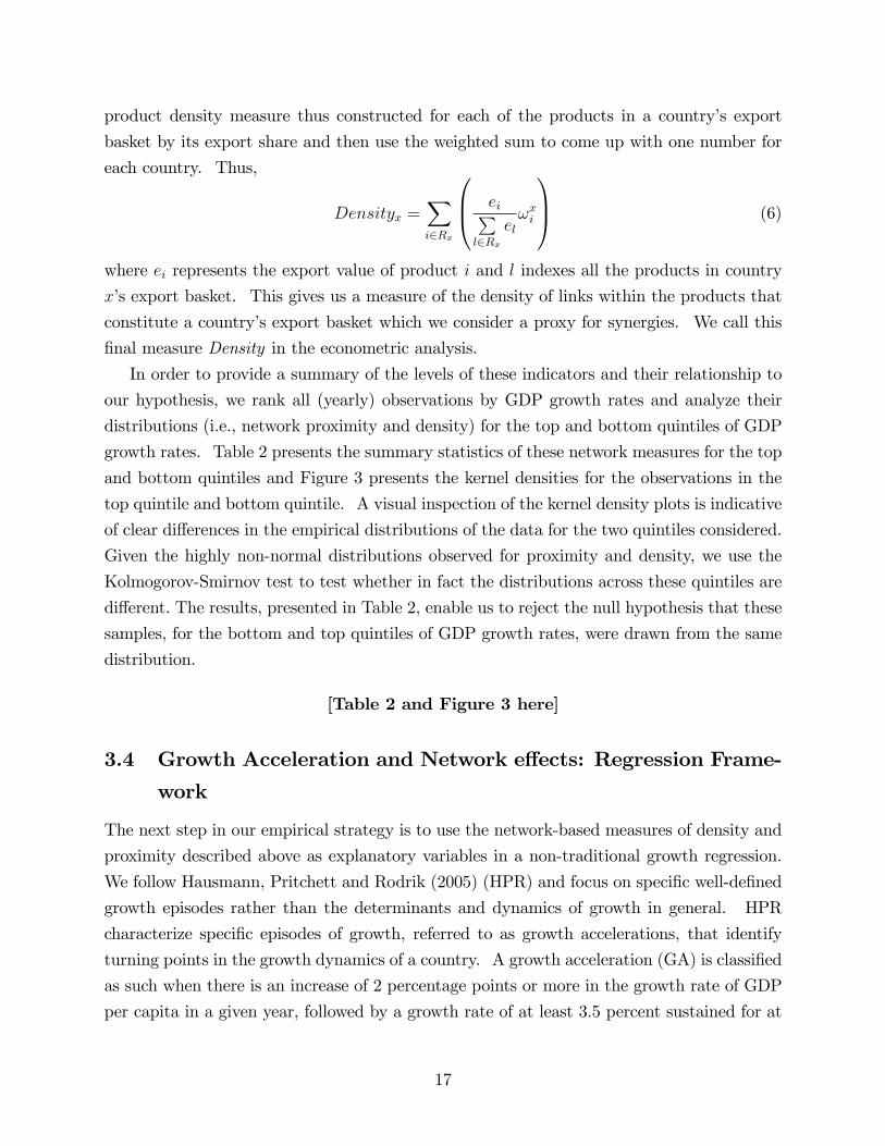
product density measure thus constructed for each of the products in a country’s export

basket by its export share and then use the weighted sum to come up with one number for

each country. Thus,

Densityx =∑i∈Rx

ei∑l∈Rx

elωxi

(6)

where ei represents the export value of product i and l indexes all the products in country

x’s export basket. This gives us a measure of the density of links within the products that

constitute a country’s export basket which we consider a proxy for synergies. We call this

final measure Density in the econometric analysis.

In order to provide a summary of the levels of these indicators and their relationship to

our hypothesis, we rank all (yearly) observations by GDP growth rates and analyze their

distributions (i.e., network proximity and density) for the top and bottom quintiles of GDP

growth rates. Table 2 presents the summary statistics of these network measures for the top

and bottom quintiles and Figure 3 presents the kernel densities for the observations in the

top quintile and bottom quintile. A visual inspection of the kernel density plots is indicative

of clear differences in the empirical distributions of the data for the two quintiles considered.

Given the highly non-normal distributions observed for proximity and density, we use the

Kolmogorov-Smirnov test to test whether in fact the distributions across these quintiles are

different. The results, presented in Table 2, enable us to reject the null hypothesis that these

samples, for the bottom and top quintiles of GDP growth rates, were drawn from the same

distribution.

[Table 2 and Figure 3 here]

3.4 Growth Acceleration and Network effects: Regression Frame-

work

The next step in our empirical strategy is to use the network-based measures of density and

proximity described above as explanatory variables in a non-traditional growth regression.

We follow Hausmann, Pritchett and Rodrik (2005) (HPR) and focus on specific well-defined

growth episodes rather than the determinants and dynamics of growth in general. HPR

characterize specific episodes of growth, referred to as growth accelerations, that identify

turning points in the growth dynamics of a country. A growth acceleration (GA) is classified

as such when there is an increase of 2 percentage points or more in the growth rate of GDP

per capita in a given year, followed by a growth rate of at least 3.5 percent sustained for at

17

least eight years, and the post-acceleration level of output exceeds the pre-acceleration peak

so as to rule out recoveries from economic crises8.

Our goal is to explain the likelihood of observing growth acceleration, and our empirical

specification uses a probit model where the dependent variable takes the value of one for

the year before which, on which, and after which a growth acceleration occurred, and zero

otherwise. Having a 3 year window to mark the growth acceleration accounts for possible

noise in the data that could lead to a miscalculation of the specific year in which the acceler-

ation took place. In addition, by focusing on these episodes many of the problems faced by

traditional growth regressions are avoided since the specific development stage of the country

loses importance; the fact that growth accelerated is the relevant information for the analysis.

The objective then becomes the identification of the conditions, policy changes, or structural

characteristics that explain the occurrence of growth acceleration episodes observed across

countries and through time.

This probit methodology is the same as that followed by HPR, but in addition to their

control variables, which account for the effect of economic reforms, terms of trade shocks

and political regime changes, we include network-based measures of density and network

proximity for each country in order to evaluate our hypothesis. We use the following

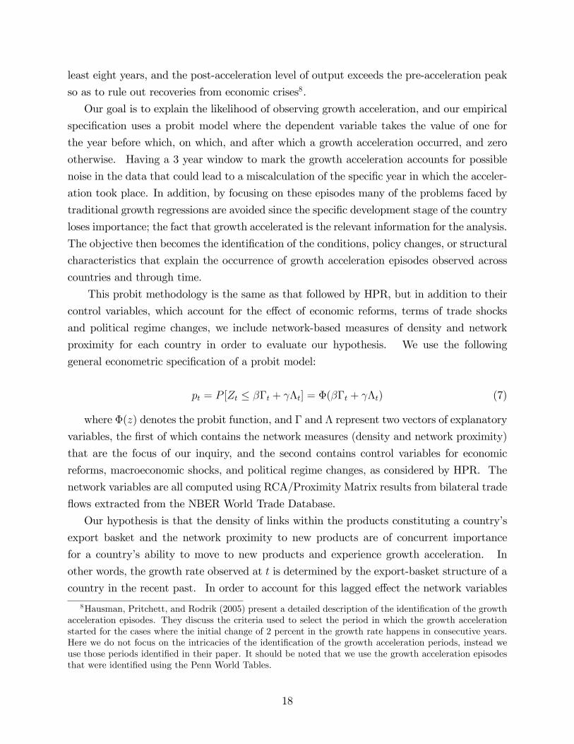
general econometric specification of a probit model:

pt = P [Zt ≤ βΓt + γΛt] = Φ(βΓt + γΛt) (7)

where Φ(z) denotes the probit function, and Γ and Λ represent two vectors of explanatory

variables, the first of which contains the network measures (density and network proximity)

that are the focus of our inquiry, and the second contains control variables for economic

reforms, macroeconomic shocks, and political regime changes, as considered by HPR. The

network variables are all computed using RCA/Proximity Matrix results from bilateral trade

flows extracted from the NBER World Trade Database.

Our hypothesis is that the density of links within the products constituting a country’s

export basket and the network proximity to new products are of concurrent importance

for a country’s ability to move to new products and experience growth acceleration. In

other words, the growth rate observed at t is determined by the export-basket structure of a

country in the recent past. In order to account for this lagged effect the network variables

8Hausman, Pritchett, and Rodrik (2005) present a detailed description of the identification of the growthacceleration episodes. They discuss the criteria used to select the period in which the growth accelerationstarted for the cases where the initial change of 2 percent in the growth rate happens in consecutive years.Here we do not focus on the intricacies of the identification of the growth acceleration periods, instead weuse those periods identified in their paper. It should be noted that we use the growth acceleration episodesthat were identified using the Penn World Tables.

18

enter the regression with lagged values based on averages across time-windows. For example,

the value of density in the dataset at time t is the average of density in periods t− 6, t− 5,

and t − 4. The reason to consider lagged-window averages is simply to better capture the

state of RCA over a certain period of time, instead of focusing just on specific points in time

that could be volatile and therefore introduce noise into the regression. The other network

variables, distance and density, also enter the regression in the same “lagged time-window

averages” fashion. For robustness, we also consider averages for t − 5, t − 4, and t − 3, as

well as for t − 7, t − 6, and t − 5, thus providing longer and shorter lagged windows for

comparisons with our benchmark regression.

In addition, our theoretical framework, involving a leap feasibility constraint and a leap

incentive constraint, suggests a non-monotonic relationship between density and network

proximity. In order to test this our econometric specification considers quadratic terms for

density and network proximity.

The economic and political control variables included in Λ in (7) match those included in

the econometric specification proposed by HPR. Specifically, these measures are proxies for

external shocks, changes in political regime, and economic reforms. All these variables enter

the regression as dummy variables. HPR compute an indicator variable based on the terms

of trade which proxies for external shocks. This variable takes the value of one whenever the

change of the terms of trade variable is in the upper ten percent from the start of the growth

acceleration in period t, to t − 4, four periods before the start of the growth acceleration.

Political regime changes have been linked to changes in the underlying fundamentals of

the economic structure of countries the have experienced them. These dramatic changes

may shift the economy to a different trajectory of economic growth that in many cases

corresponds to higher rates of growth. These political regime changes are identified in the

HPR dataset by using the Polity IV data provided by Marshall and Jaggers (2002). The

corresponding dummy variable in the econometric specification takes the value of one in

the five periods following a regime change, which is defined as a change of at least three

units in the polity score, or by a regime interruption. Finally, the economic reform variables

control for trade and financial liberalization episodes. Opening an economy to trade and

financial flows provides access to markets, competition, and a better allocation of resources

that leads to an improved economic environment that, in theory, results in higher rates of

growth. Pin-pointing the exact periods in which a country is opened up for free trade and

financial flows is not an easy task. Wacziarg and Welch (2003) have updated and expanded

the index proposed by Sachs and Warner (1995) which incorporates several dimensions of

the structural fundamentals of a country’s economic system. The index controls for foreign

currency black market premiums, levels of tariffs, and other trade barriers. HPR use it as

19

an indicator of transition towards trade openness. The dummy variable included in our

regression that uses the information derived from this index takes the value of one during

the five years after a transition towards openness has occurred9.

4 Regression Results and Analysis

Our probit regression starts by replicating the HPR specification as a baseline for our analy-

sis. Columns 1 and 2 in Table 3 present the results for the core specification presented in

HPR. Column 1 reports the results using the exact same sample (countries and years) in-

cluded in their analysis, while column 2 presents results from the reduced sample (countries

and years) used in this study. The changes in the sample come from data constraints arising

from the computation of RCA and corresponding network variables for as many countries

and years as possible. We see that the statistical significance and the magnitude of the

coeffi cients from our sub-sample are very close to those of the original sample, suggesting

that the loss of observations due to limited data on the RCA based variables does not af-

fect the fundamentals of the analysis, and validates comparison of our results with those of

HPR. The marginal effect10 of external shocks (measured through the terms of trade) and

regime change on the probability of experiencing a growth acceleration, computed from the

estimated coeffi cients in column 1, are 4.4 and 5.3 percentage points respectively, essentially

replicating HPR’s results for the same specification.

[Table 3 here]

Columns 3 and 4 in Table 3 present results for the econometric specifications that test the

implications of our hypothesis. Column 3 presents the probit regression coeffi cients obtained

for the econometric specification that only explores linear effects of the network indicators.

When no consideration is given for non-linear effects, we see that the results point to the

statistical significance of density and network proximity, but the estimated coeffi cient for

density is negative. The estimated coeffi cient for network proximity is positive, and the

coeffi cients of the HPR variables remain virtually unchanged.

However, what is missing in the empirical specification of column 3 is the consideration

that the network variables can have non-monotonic effects due to the way in which they may

interact via the constraints in the leap mechanism described earlier. Recall from section 2

that the theoretical mechanism involves two constraints: a leap feasibility constraint and a

9Where "transition towards openness" is defined a la Sachs-Warner-Wacziarg-Welch, based on theWacziarg and Welch (2003) updated index from Sachs and Warner (1995).10Evaluated as in HPR.

20

leap incentive constraint. The leap feasibility constraint implies that if network proximity

goes down (raising the costs of leaping to a new product) then density needs to go up (en-

hancing cost-reducing synergies and freeing up resources) to ensure leap feasibility. The leap

feasibility constraint thus suggests a negative relationship between network proximity and

density. The leap incentive constraint implies that if current synergies are high this creates

inertia since current synergies will be lost if a leap is made to a new part of the proximity

matrix where new synergies take time to develop. If this is the case then network proximity

needs to also be high in order to ensure there is a leap incentive. The leap incentive con-

straint thus suggests a positive relationship between density and network proximity. Putting

the two constraints together then implies that whether the relationship between density and

network proximity is positive or negative depends on whether the leap incentive constraint

or the leap feasibility constraint is respectively binding. There can thus be a non-linear

relationship between density and network proximity. Given these considerations, we expand

the econometric specification to include quadratic terms of the network indicators.

Specification 4 in Table 3 presents the regression results for the specification that includes

the linear and quadratic terms for density and network proximity simultaneously. The coef-

ficients for the linear effects of density and network proximity are still statistically significant

but their signs are opposite to those reported in the case where only the linear effects were

controlled for in the econometric specification. Both quadratic terms are significant as well,

positive for network proximity and negative for network density. These results support the

argument for non-monotonicity but also require an expanded interpretation of the effects of

the network indicators on the likelihood of growth acceleration.

A clean and intuitive interpretation for the results of the country-level effects can be

obtained by evaluating the estimated probit function for all the possible levels of density and

network proximity, while keeping the other control variables at their means. In other words,

we can build a grid of all the possible combinations for density and network proximity and

evaluate the probability function at each point. This exercise enables us to see if the effects

of these variables establish a distinct region where the probability of growth acceleration is

high, and if this region conforms with the intuition of our hypothesis.

Figure 4 presents the results for the grid of density and network proximity, using the

relevant ranges in our dataset to evaluate the econometric specification presented in column 4

of Table 3. The right-hand panel of the figure presents a 3-D view of the probability function

while the left-hand panel presents a birds-eye view. From the left-hand panel we see that the

shape of the high probability region (indicated by the black zone) resembles an arc. There

is a high probability segment where density and network proximity are negatively related.

This relationship emerges for density levels of up to values of 0.20. The relationship between

21

density and network proximity becomes positive for density values greater than 0.20. Recall

that the discussion of the leap mechanism in section 2 argues that at low values of density it is

likely that the leap feasibility constraint will bind, leading us to expect a negative relationship

between density and network proximity, and at high values of density it is likely that the leap

incentive constraint will bind, leading us to expect a positive relationship between density

and network proximity. The shape of the high probability arc is in accordance.

We also see that the probability of growth acceleration falls off quite sharply outside

of the arc region. In order to get a sense of the magnitude of changes in the probability

levels brought about by changes in network proximity it is helpful to pick a value for density

(keeping the other control variables at their means). For example, holding density at 0.20,

the highest probability (39.8%) of growth acceleration is achieved when network proximity

is 0.238. If network proximity decreases by one standard deviation (0.047) the probability

drops by almost 10 percentage points, and if network proximity decreases by two standard

deviations the probability decreases by almost 21 percentage points.

[Figure 4 here]

We should also note that the results presented here are robust and do not vary signifi-

cantly when other control variables are considered. For example, when controls for financial

liberalization are included in the regression analysis as in HPR, the statistical significance

of the linear and quadratic terms, and the arc shape of the high probability region persist.

We also explore the robustness of our results by considering different lags for the compu-

tation of the network variables. The specification in column 4 of Table 3 used averages of

the variables for periods t−6, t−5, and t−4. We consider two alternative lagged structures,

one that uses averages of periods t − 5, t − 4, and t − 3, and a second one that computes

averages of periods t − 7, t − 6, and t − 5. The results for these alternative (averaged)

network variables are presented in columns 5 and 6, respectively, on the same table. We see

that the statistical significance and the signs for density, network proximity for both linear

and quadratic terms persist.

In summary, our regression results provide statistical support for the hypothesis. The

non-linear effects reported seem to be robust to different lagged structures and are consistent

with the intuition from our hypothesis.

Finally, we should reiterate that we focus on sharp transitions in the growth path rather

than economic growth per-se because the mechanism we have in mind pertains to the ability

of a country to move to new products and change its production structure. Such a change

should have a discrete effect on economic growth, if it does have an effect at all. An increase

in the economic growth rate is a long-run effect, a complex phenomenon to which we do

22

not have much new to add in this paper. Nonetheless, we examine whether the network

measures developed here explain country level growth rates. To verify our focus, we investi-

gated if the network measures developed in our paper explain country level growth rates in

a more traditional growth regression model. To that end we developed an empirical growth

regression model that incorporates our network measures. We regressed average annual

growth rate from t to t+5 on our network measures calculated over the period t-2 to t.

We also include country level controls that are included in standard trade-growth analyses

such as Yanikkaya (2003). We estimate this model using our country level panel dataset.

Our estimations indicate that our network measures do not have much predictive power for

country level GDP growth. None of the network measures were statistically significant in

the growth regressions. The coeffi cient estimates for the control variables and the predictive

power of the model as a whole are mostly consistent with growth regression specifications

present in the literature. This result leads us to believe that while our network measures

are good predictors of growth accelerations, they do not add much to the standard growth

specification. A possible explanation could be that while many economies are continually

taking many small steps in the evolution of their production structure on a regular basis,

these incremental changes arguably do not have an impact on the likelihood of a growth ac-

celeration until they coalesce into a big change, due to supermodularity and complementarity

considerations.

5 Conclusion

While consensus on the trade-growth nexus is in disarray, recent research continues to paint

a favorable picture of outward-oriented policy reforms on average while cautioning against a

one-size-fits-all policy that disregards local circumstances. Focus has therefore shifted to a

scrutiny of the channels through which trade openness may influence economic performance,

and the way in which the relationship between trade and growth is contingent on country

and external characteristics. Our paper contributes to this literature by identifying a new

mechanism which facilitates transition to a high growth path.

We focus on the relationship between products in global trade and the characteristics

of a country’s pattern of product specialization as revealed through its exports. Explicitly

mapping the proximity matrix as a network and then superimposing a country’s pattern of

product specialization on the proximity matrix enables us to devise a measure of the density

of links between the products in a country’s export basket and a measure of how close a

country’s product specialization pattern is to the rest of product space. We use the density

measure as a proxy for synergies between the products in a country’s export basket. The

23

network proximity measure gives us an indicator of how diffi cult it is likely to be for a given

country to move from its current product specialization to new products. Our hypothesis

is that the density of links within the products constituting a country’s export basket and

the network proximity to new products are of concurrent importance for a poor country to

move to higher income products and thus higher growth rates.

We provide evidence in support of this hypothesis. Our network measures are signifi-

cant in predicting a heightened probability of experiencing subsequent growth acceleration.

We use the combinations of density and network proximity from our data in conjunction

with the estimated coeffi cients from the probit regression to build a grid of the probability

function at each point. This exercise demonstrates that the shape of the high probability

region resembles an arc. The arc implies that our measure of the density of links between

products and network proximity to new products are related in a non-monotonic fashion

for a heightened probability of experiencing a growth acceleration. We also find that the

probability of growth acceleration falls off quite sharply outside of the arc traced by this

exercise.

The network-based methodology unravels characteristics of the growth acceleration process

that are diffi cult to both see and understand using conventional approaches. In this sense,

the methodology itself can expand the scope of the questions that we will be able to ask.

For example, the literature on complex networks proposes many ways in which the favorable

configuration may arise (short-cuts, hubs, modularity). This in turn suggests that a number

of different policies or historical accidents could lead to this configuration and therefore to

conditions that are propitious for growth acceleration. It is important to note that the pre-

ceding analysis says nothing about the process by which such conditions arise in countries.

This is a promising area for future research.

24

References

[1] Albert, A. and A. L. Barabasi, (2002), “Statistical Mechanics of Complex Networks”,

Reviews of Modern Physics 74, 47.

[2] Barabasi, A. (2002), Linked: The New Science of Networks, Perseus Publishing, Cam-

bridge, MA.

[3] Ben-David, D. (1993), “Equalizing Exchange: Trade Liberalization and Income Con-

vergence,”Quarterly Journal of Economics, 108(3): 653-79.

[4] Castilla, E. J., H. Hwang, E. Granovetter, and M. Granovetter, “Social Networks in

Silicon Valley,” in C.-M. Lee, W. F. Miller, M. G. Hancock, and H. S. Rowen (eds.),

The Silicon Valley Edge, Stanford: Stanford University Press.

[5] Dollar, D. (1992), “Outward-Oriented Developing Economies Really Do Grow More

Rapidly: Evidence from 95 LDC’s, 1976-85,” Economic Development and Cultural

Change, 40: 523-44.

[6] Ellison, G. and E. Glaeser (1997), “Geographic Concentration in U.S. Manufacturing

Industries: A Dartboard Approach,”Journal of Political Economy, 105: 889-927.

[7] Ellison, G., E. Glaeser and Kerr (2010), “What Causes Industry Agglomeration? Ev-

idence from Coagglomeration Patterns,”American Economic Review, vol. 100, June,

pp. 1195-1213.

[8] Feenstra, R. C., R.E. Lipsey, Deng, H., Ma, A.C. and Hengyong Mo, (2005),“World

Trade Flows, 1962-2000,”NBER Working Paper 11040.

[9] Frankel, Jeffrey A. and David Romer (1999), “Does Trade Cause Growth?”American

Economic Review, vol. 89, no. 3, pp. 379-399.

[10] Glaeser, E. L., H. D. Kallal, J. A. Scheinkman, and A. Shleifer (1992), “Growth in

Cities,”Journal of Political Economy, 100: 1126-1152.

[11] Goyal, S. (2008), Connections: An introduction to the economics of networks, Prince-

ton University Press.

[12] Goyal, S., M. J. van der Leij (2006), “Economics: An Emerging Small World,”Journal

of Political Economy, 11(2): 403-412.

25

[13] Grossman, G. and E. Helpman (1991), Innovation and Growth in the Global Economy,

MIT Press, Cambridge, MA.

[14] Hausmann, Ricardo, Lant Prichett, and Dani Rodrick (2005), "Growth Accelerations,"

Journal of Economic Growth, 10(4): 303-329.

[15] Hausmann, R. and B. Klinger (2007), “The Structure of the Product Space and the

Evolution of Comparative Advantage,”Working Paper, Kennedy School, Harvard Uni-

versity.

[16] Hidalgo, C. and R. Hausmann (2009), “The building blocks of economic complexity,”

Proceedings of the National Academy of Sciences, 106(26): 10570-10575.

[17] Hidalgo, C.A., Klinger, B., Barabasi, A.L. and R. Hausmann (2007), “"The Product

Space Conditions the Development of Nations,”Science, 27 July 2007, Vol 317: 482-487.

[18] Hirschman, A. (1958), The Strategy of Economic Development, New Haven, Conn.:

Yale University Press.

[19] Jaccard, P. (1901) Étude comparative de la distribution florale dans une portion des

Alpes et des Jura. Bulletin del la Société Vaudoise des Sciences Naturelles 37, 547-579.

[20] Jackson, M. (2009), Social and Economic Networks, Princeton University Press.

[21] Jackson, M. O. (2006), “The Economics of Social Networks,”in Advances in Economics

and Econometrics, Theory and Applications: Ninth World Congress of the Econometric

Society, edited by Richard Blundell, Whitney Newey, and Torsten Persson, Chapter 1,

Volume I, Cambridge University Press.

[22] Jacobs, J. (1984), Cities and the Wealth of Nations: Principles of Economic Life, New

York: Random House.

[23] Krueger, A. O. (1998), “Why Trade Liberalisation is Good for Growth,” Economic

Journal, 108: 1513-1522.

[24] Matsuyama, Kiminori (1992), “Agricultural Productivity, Comparative Advantage, and

Economic Growth”, Journal of Economic Theory, vol. 58, no. 2, pp. 317-334.

[25] Newman, M. E. J. (2003), “The Structure and Function of Complex Networks”, SIAM

Review 45, 167-256.

[26] Pang-Ning T, M. Steinbach and V. (2005), Introduction to Data Mining, ISBN 0-321-

32136-7.

26

[27] Rodriguez-Claire, A. (2007), “Clusters and comparative advantage: Implications for

industrial policy,”Journal of Development Economics, 82:43-57.

[28] Rodriguez, Francisco and Dani Rodrik (2001), “Trade Policy and Economic Growth: A

Sceptic’s Guide to the Cross-National Evidence”, NBER Macroeconomics Annual 2000.

Cambridge, MA: MIT Press, pp. 261-324.

[29] Ruan, J. and W. Zhang (2008), “Identifying network communities with a high resolu-

tion,”Physical Review E, 77 016104:1-12.

[30] Sachs, J. and A. Warner (1995), “Economic Reform and the Process of Global Integra-

tion,”Brookings Papers on Economic Activity, 1: 1-118.

[31] Saxenian, A. (1994), Regional Advantage: Culture and Competition in Silicon Valley and Route 128,

Cambridge, Massachusetts: Harvard University Press.

[32] Wacziarg, R. and K. H. Welch (2008), “Trade Liberalization and Growth: New Evi-

dence,”World Bank Economic Review, 22(2): 187-231.

[33] Watts, D. J. and S. H. Strogatz. (1998) “Collective Dynamics of ‘Small-World’Net-

works”, Nature 393:440-442.

[34] Watts, D. (2003), Six Degrees: The Science of a Connected Age, W.W. Norton, New

York & London.

[35] Yanikkaya, H. (2003), “Trade Openness and Economic Growth: A Cross-Country Em-

pirical Investigation,”Journal of Development Economics, 72, 57 —89.

27

28

Figure 1 Jaccard Index

2000 = Benchmark 1985 = Benchmark

Notes: We use the QCut community structure algorithm to identify communities into which the proximity matrix is partitioned for every year. We then compare the community structures of each year against a given benchmark (2000 in the left panel and 1985 in the right panel) using the Jaccard Index (similarity coefficient). The Jaccard Index equals zero for the case where the community structures compared are completely different, and it is equal to one for the case where they are exactly equivalent community structures. The base years are not included in the graphs above.

Figure 2. Graph Partitioning of Product Space (Color-coded representation)

Notes: The figures depict the product space partitioned into 10 pre-specified communities. The communities are pre-specified according to one-digit SITC industry codes. The color-coded graph partitioning matrices for 1970 and 2000 in Figure 2 provide an overview of the evolution of the proximity matrix at the industry level (1-digit SITC), where the value in each cell of the matrices represents the sum of the valued interactions (i.e., proximities) between the corresponding products considered at the 4-digit level by cluster, in other words the data is aggregated from the 4-digit level to the 1-digit level. The values in each of the cells on the diagonal of these matrices represent the sum of the interactions of all the products (4-digit level) within the same industry (1-digit level), while the off diagonal cells present the sum of the interactions between products of diffferent industries. The two different panels in Figure 2 present a visual illustration of these valued matrices using a continuous gray scale to denote the different values of these interactions. Higher valued interactions within and across industries are denoted by darker shades of gray.

Product Space (1-digit SITC)Partition2000

Industry Clusters (1-digit SITC codes)

Indu

stry

Clu

ster

s (1

-dig

it S

ITC

cod

es)

2 4 6 8 10

1

2

3

4

5

6

7

8

9

100.01

0.02

0.03

0.04

0.05

0.06

0.07

0.08

0.09

0.1

0.11

Product Space (1-digit SITC)Partition1970

Industry Clusters (1-digit SITC codes)

2 4 6 8 10

1

2

3

4

5

6

7

8

9

10

0.01

0.02

0.03

0.04

0.05

0.06

0.07

0.08

0.09

0.1

0.11

SITC 0 ==>

SITC 1 ==>

SITC 2 ==>

SITC 3 ==>

SITC 4 ==>

SITC 5 ==>

SITC 6 ==>

SITC 7 ==>

SITC 8 ==>

SITC 9 ==>

0

0.1

0.2

0.3

0.4

0.5

0.6

0.7

1962 1965 1970 1975 1980 1985 1990 1995

Jacc

ard

Inde

x

0

0.1

0.2

0.3

0.4

0.5

0.6

0.7

1962 1965 1970 1975 1980 1990 1995 2000

Jacc

ard

Inde

x

29

Figure 3. Kernel Density Plots

Notes: The figures present the kernel density plots of the network indicators for the top quintile and the bottom quintile, ranked according to GDP growth rates, using all yearly observations.

Figure 4. Probit Function: Evaluated for all Possible Combinations of Density and Network Proximity

Notes: Estimated probabilities computed by evaluating the econometric specification presented in column 4 of

Table 3, ][ tttt ZPp Λ+Γ== γβ , using the relevant ranges in the dataset for density and network proximity in levels and squared terms in the vector of network measures,Γ , and the mean values for all other control variables in the vector of economic reform variables, Λ . The right-hand panel of the figure presents a 3-D view of the probability function while the left-hand panel presents a birds-eye view.

0

400

800

1,200

1,600

2,000

.0095 .0100 .0105 .0110 .0115 .0120 .0125 .0130 .0135 .0140 .0145 .0150

Network Proximity Top QuintileNetwork Proximity Bottom Quintile

Kern

el D

ensi

ty

0

1

2

3

4

5

6

7

-.1 .0 .1 .2 .3 .4 .5 .6

Density Top QuintileDensity Bottom Quintile

Kern

el D

ensi

ty

30

Table 1. Correlation between Product Space and Country Level Product Specialization 1980 1990

Honduras 0.346

0.205 Bolivia 0.422

0.242

Paraguay 0.188

0.255 Argentina 0.256

0.293

Egypt 0.335

0.375 Peru 0.524

0.384

Uruguay 0.506

0.464 Indonesia 0.115

0.475

Colombia 0.633

0.494 Thailand 0.596

0.580

Greece 0.669

0.585 Singapore 0.713

0.609

Netherlands 0.732

0.615 Canada 0.823

0.679

India 0.771

0.712 Portugal 0.815

0.713

USA 0.857

0.724 Japan 0.868

0.747

Belgium 0.822

0.777 South Korea 0.811

0.780

Malaysia 0.571

0.796 Ireland 0.888

0.820

Brazil 0.812

0.828 Spain 0.858

0.875

Hungary 0.830

0.882 UK 0.958

0.934

Mexico 0.813

0.943 Germany 0.941

0.946

France 0.948

0.954 Poland 0.834 0.956

Notes: The table presents the correlation coefficients for 1980 and 1990 between the information matrix for the pattern of product specialization of a given country and the information matrix for the complete proximity matrix. These matrices result from aggregating the data from the 4-digit SITC level to the 1-digit SITC product level (industry level), such that the matrix used corresponds to the 10 SITC based clusters described in the paper. Each of the cells of the resulting matrices presents the sum of all the interactions that exist between each product at the 4-digit SITC level that corresponds to the industries considered (1-digit SITC level). The diagonal corresponds to the sum of interactions between products of the same SITC industry, while the cells off the diagonal correspond to sum of interactions between industries. A correlation level close to zero suggests that the industry level of interaction for a given country does not match with that observed for the complete proximity matrix, On the other extreme a correlation close to one would signal a large degree of similarity between the levels of industry interactions of a given country and those observed for the complete proximity matrix.

31

Table 2. Summary Statistics for Network Measures (Top and Bottom Quintiles of the data Ranked by GDP growth rates)

Bottom Quintile Top Quintile K-S test (D)

Density Mean 0.15 0.19 0.2735* Std. dev 0.07 0.09

Network Proximity Mean 0.048 0.072 0.2374* Std. dev 0.047 0.057

Obs 526 475 Notes: All yearly observations for the network indicators are sorted according to the observed GDP growth rates. The table presents the descriptive statistics of the network indicators for the top and bottom quintiles. The K-S test rejects the null hypothesis that density and network proximity series for the bottom and top quintiles are drawn from the same distribution. . * Statistical significance at the 1% level.

Table 3. Regression Results

4

Density -2.73 ** 11.40 *** 11.54 *** 6.12 **

-2.25 3.32 3.78 2.26

Network Proximity 4.100 ** -9.48 ** -11.680 *** -7.152 *

2.17 -2.37 -2.83 -1.79

Density^2 -30.29 *** -32.20 *** -18.88 ***

-3.78 -4.62 -3.12

Network Proximity^2 55.26 *** 63.90 *** 44.24 ***

3.88 4.51 3.35

Terms of Trade 0.30 ** 0.35 ** 0.36 *** 0.34 ** 0.32 ** 0.35 **

2.43 2.56 2.71 2.50 2.39 2.56

Liberalization 0.16 0.20 0.19 0.17 0.17 0.18

1.03 1.24 1.24 1.06 1.16 1.10

Regime Change 0.40 *** 0.34 *** 0.32 *** 0.29 *** 0.33 *** 0.33 ***

4.59 3.60 3.46 3.13 3.45 3.45

Pseudo R-squared 0.0392 0.0364 0.0409 0.064 0.0728 0.0623

No. Obs. 2140 1748 1748 1748 1707 1707

Notes: Results for the Probit regressions.Density and Network proximity are the network indicators included in the vector of network measures, Γ, use to control for the degreeof overlap of a country's pattern of product specialization and the rest of the product space. Linear and cuadratic terms are inlcuded in order control for non-linearities. Standard variables are included to control for political regime changes (Regime Change), opening the economy for trade (Liberalization), and terms of trade shocks (Terms of Trade). These are included in the vector of other controls, Λ.Notes: *,**, and *** denote statistical significance at the 10, 5 and 1 percent confidence levelsz-statistics for the coefficients appear in italics.

6 (t-7, t-6, t-5)

Robustness1 2 3 5

(t-5, t-4, t-3)

][ tttt ZPp Λ+Γ== γβ

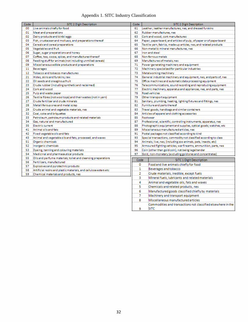
32

Appendix 1. SITC Industry Classification