Growth mixture models in longitudinal research · Growth mixture models in longitudinal research...

AStA Adv Stat Anal (2011) 95:415–434DOI 10.1007/s10182-011-0171-4

O R I G I NA L PA P E R

Growth mixture models in longitudinal research

Jost Reinecke · Daniel Seddig

Received: 20 August 2010 / Accepted: 3 March 2011 / Published online: 19 October 2011© Springer-Verlag 2011

Abstract Latent growth curve models as structural equation models are extensivelydiscussed in various research fields (Curran and Muthén in Am. J. Community Psy-chol. 27:567–595, 1999; Duncan et al. in An introduction to latent variable growthcurve modeling. Concepts, issues and applications, 2nd edn., Lawrence Earlbaum,Mahwah, 2006; Muthén and Muthén in Alcohol. Clin. Exp. Res. 24(6):882–891,2000a; in J. Stud. Alcohol. 61:290–300, 2000b). Recent methodological and sta-tistical extension are focused on the consideration of unobserved heterogeneity inempirical data. Muthén extended the classic structural equation approach by mix-ture components, i.e. categorical latent classes (Muthén in Marcouldies, G.A., Scku-macker, R.E. (eds.), New developments and techniques in structural equation model-ing, pp. 1–33, Lawrance Erlbaum, Mahwah, 2001a; in Behaviometrika 29(1):81–117,2002; in Kaplan, D. (ed.), The SAGE handbook of quantitative methodology for thesocial sciences, pp. 345–368, Sage, Thousand Oaks, 2004). The paper discusses ap-plications of growth mixture models with data on delinquent behavior of adolescentsfrom the German panel study Crime in the modern City (CrimoC) (Boers et al. in Eur.J. Criminol. 7:499–520, 2010; Reinecke in Delinquenzverläufe im Jugendalter: Em-pirische Überprüfung von Wachstums- und Mischverteilungsmodellen, Institut fürsozialwissenschaftliche Forschung e.V., Münster, 2006a; in Methodology 2:100–112,2006b; in van Montfort, K., Oud, J., Satorra, A. (eds.), Longitudinal models in thebehavioral and related sciences, pp. 239–266, Lawrence Erlbaum, Mahwah, 2007).Observed as well as unobserved heterogeneity will be considered with growth mix-ture models. Special attention is given to the distribution of the outcome variables as

J. Reinecke (�)Faculty of Sociology, University of Bielefeld, Bielefeld, Germanye-mail: [email protected]

D. SeddigDepartment of Criminology, University of Münster, Münster, Germanye-mail: [email protected]

mailto:[email protected]

mailto:[email protected]

416 J. Reinecke, D. Seddig

counts. Poisson and negative binomial distributions with zero inflation are consideredin the proposed growth mixture models variables. Different model specifications willbe emphasized with respect to their particular parameterizations.

Keywords Panel data · Latent class growth analysis · Growth mixture modeling ·Heterogeneity · Zero-inflated negative binomial model

1 Introduction

Longitudinal research studies with repeated measurements are quite often used to ex-amine processes of stability and change in individuals or groups. With panel data itis possible to investigate intraindividual development of substantive variables acrosstime as well as interindividual differences and similarities in change patterns. Whilethe traditional analysis of variance (ANOVA) and the analysis of covariance (AN-COVA) assume homogeneity of the underlying covariance matrix across the levelsof the between-subjects factors and the same covariance patterns for the repeatedmeasurements, the structural equation methodology offers an alternative strategy: thelatent growth curve models. These models describe not only a single individual’s de-velopmental trajectory, but also capture individual differences in the intercept andslopes of those trajectories. Based on the formative work of Rao and Tucker’s basicmodel of growth curves (Rao 1958; Tucker 1958), Meredith and Tisak (1990) dis-cussed and formalized the model within the structural equation framework. Furtherdevelopments of the growth curve model were proposed by McArdle and Epstein(1987), McArdle (1988) and Muthén (1991, 1997).

Observed heterogeneity in growth curve models can be captured by covariatesexplaining part of the variances of the intercept and slope. But the assumption ofa single population underlying the growth curves has to be relaxed in the case ofunobserved heterogeneity. Instead of considering individual variation around a sin-gle growth curve, different classes of individuals should vary around different meangrowth curves. A very suitable framework to handle the issue of unobserved het-erogeneity is growth mixture modeling introduced by Muthén and Shedden (1999).These mixture models differ between continuous and categorical latent variables. Thecategorical latent variables represent mixtures of subpopulations where the productmembership is inferred from the data. Like the conventional growth curve models,intercept and slope variables capture the continuous part of the model. Growth mix-ture models can also be seen as an extension of the structural modeling approachwith techniques of latent class analysis. The inferred membership of each individualto a certain class is produced with the information of the estimated latent class prob-abilities. Further developments and applications with the program Mplus (Muthénand Muthén 2006) are discussed in several papers by Muthén (2001a, 2001b, 2003,2004). Recently, Muthén (2008) gives a model overview of the so-called latent vari-able hybrids within the continuous and categorical latent variable framework.

Statistical techniques to group and classify individuals with categorical panel data(e.g., latent class analysis) have a long tradition in behavioral and social sciences(Rost and Langeheine 1997). In criminology, classification of longitudinal contin-uous and count data were formally introduced by Nagin and Land (1993), Nagin

Growth mixture models in longitudinal research 417

(1999) and Roeder, Lynch and Nagin (1999) with the semiparametric group-basedapproach (see also Nagin 2005 for an overview). This technique enhanced the abilityto estimate group membership of individuals who follow a common trajectory acrosstime (e.g., persistent offenders). Muthén (2004) discusses this group-based approachas a simpler specification of the general growth mixture model and labeled it as latentclass growth analysis. In difference to the general growth mixture model the growthcurve parameters are fixed and not random, assuming no variation across individualswithin classes. The possibility to treat their measurements as counts with the Poissondistribution as the underlying statistical model (see, e.g., Ross 1993) is also part of themixture model. If the count variables are inflated with zeros, i.e. the particular behav-iors seldom occur, a variant of the Poisson model, the so-called zero-inflated Poissonmodel (ZIP, Lambert 1992) should lead to a better statistical representation of the datathan a model without considering the zero inflation. However, a Poisson distributionassumes the equality of its mean and variance. This property is rarely found in em-pirical data. If the variance is larger than the mean, then the negative binomial model(NB) should be used instead of the Poisson model to get a parameter estimate of theoverdispersion (cf. Hilbe 2007 for an overview of the varieties of negative binomialmodels). If the count variables are both inflated with zeros and overdispersed, the so-called zero-inflated negative binomial model (ZINB, Hilbe 2007, p. 174f.) should beapplied. The recent version of the Mplus program allows the specification of differ-ent count data models including the ZIP- and the ZINB model (Muthén and Muthén2010). The paper will focus on the applicability of zero-inflated count data modelswhich has been seldom used within growth mixture analyses.

After a short introduction of growth curve and growth mixture models, specialcases for count data are discussed in Section 2. Section 3 gives a brief introductionof the longitudinal study, the sample and the variables used in the statistical analyses.Results of the growth curve and growth mixture models are presented in Sections 4and 5. A summary and discussion with suggestions for further research are given inSection 6.

2 Method and models

2.1 Growth curve models

The possibility that the individual trajectories of a dependent variable can vary is oneof the main advantages of the growth curve model. The formal representation of agrowth curve model can be seen either as a multilevel, random-effects model or asa latent variable model, where the random effects are latent variables (Meredith andTisak 1990, p. 108; Willet and Sayer 1994, p. 369):

yi = Ληi + εi (1)

yi is a t × 1 vector of repeated measurements for observation i where t is the numberof panel waves. η is a q × 1 vector of latent growth factors where q is the numberof these factors. ε is a t × 1 vector of time-specific measurement errors, and Λ is thet ×q matrix of factor loadings with fixed coefficients representing the functional form


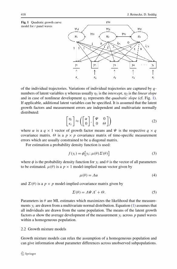
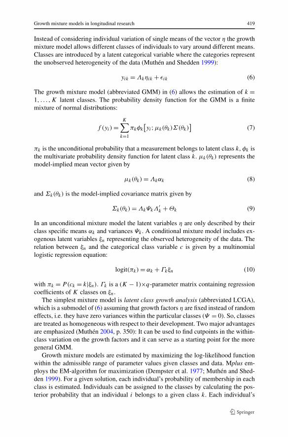
Fig. 1 Quadratic growth curvemodel for t panel waves

of the individual trajectories. Variations of individual trajectories are captured by q-numbers of latent variables η whereas usually η1 is the intercept, η2 is the linear slopeand in case of nonlinear development η3 represents the quadratic slope (cf. Fig. 1).If applicable, additional latent variables can be specified. It is assumed that the latentgrowth factors and measurement errors are independent and multivariate normallydistributed: [

ηi

εi

]≈

([α

0

],

[Ψ 00 Θ

])(2)

where α is a q × 1 vector of growth factor means and Ψ is the respective q × q

covariance matrix. Θ is a p × p covariance matrix of time-specific measurementerrors which are usually constrained to be a diagonal matrix.

For estimation a probability density function is used:

f (yi) = φ[yi;μ(θ)Σ(θ)

](3)

where φ is the probability density function for yi and θ is the vector of all parametersto be estimated. μ(θ) is a p × 1 model-implied mean vector given by

μ(θ) = Λα (4)

and Σ(θ) is a p × p model-implied covariance matrix given by

Σ(θ) = ΛΨ Λ′ + Θ. (5)

Parameters in θ are ML estimates which maximizes the likelihood that the measure-ments yi are drawn from a multivariate normal distribution. Equation (1) assumes thatall individuals are drawn from the same population. The means of the latent growthfactors α show the average development of the measurement yi across p panel waveswithin a homogeneous population.

2.2 Growth mixture models

Growth mixture models can relax the assumption of a homogeneous population andcan give information about parameter differences across unobserved subpopulations.


Instead of considering individual variation of single means of the vector η the growthmixture model allows different classes of individuals to vary around different means.Classes are introduced by a latent categorical variable where the categories representthe unobserved heterogeneity of the data (Muthén and Shedden 1999):

yik = Λkηik + εik (6)

The growth mixture model (abbreviated GMM) in (6) allows the estimation of k =1, . . . ,K latent classes. The probability density function for the GMM is a finitemixture of normal distributions:

f (yi) =K∑

k=1

πkφk

[yi;μk(θk)Σ(θk)

](7)

πk is the unconditional probability that a measurement belongs to latent class k, φk isthe multivariate probability density function for latent class k. μk(θk) represents themodel-implied mean vector given by

μk(θk) = Λkαk (8)

and Σk(θk) is the model-implied covariance matrix given by

Σk(θk) = ΛkΨkΛ′k + Θk (9)

In an unconditional mixture model the latent variables η are only described by theirclass specific means αk and variances Ψk . A conditional mixture model includes ex-ogenous latent variables ξn representing the observed heterogeneity of the data. Therelation between ξn and the categorical class variable c is given by a multinomiallogistic regression equation:

logit(πk) = αk + Γkξn (10)

with πk = P(ck = k|ξn). Γk is a (K − 1)×q-parameter matrix containing regressioncoefficients of K classes on ξn.

The simplest mixture model is latent class growth analysis (abbreviated LCGA),which is a submodel of (6) assuming that growth factors η are fixed instead of randomeffects, i.e. they have zero variances within the particular classes (Ψ = 0). So, classesare treated as homogeneous with respect to their development. Two major advantagesare emphasized (Muthén 2004, p. 350): It can be used to find cutpoints in the within-class variation on the growth factors and it can serve as a starting point for the moregeneral GMM.

Growth mixture models are estimated by maximizing the log-likelihood functionwithin the admissible range of parameter values given classes and data. Mplus em-ploys the EM-algorithm for maximization (Dempster et al. 1977; Muthén and Shed-den 1999). For a given solution, each individual’s probability of membership in eachclass is estimated. Individuals can be assigned to the classes by calculating the pos-terior probability that an individual i belongs to a given class k. Each individual’s


posterior probability estimate for each class is computed as a function of the param-eter estimates and the values of the observed data.

Standard errors of estimates are asymptotically correct if the underlying mixturemodel is the true model. In general, test statistics require well-defined classes in amixture model. In mixture models a k class model is not nested within a k + 1class model. Therefore, χ2-differences cannot be used for statistical tests. Usually,the Bayesian Information Criterion (BIC; Schwarz 1978) are used for model com-parisons which was found to perform best for growth mixture models in a simulationstudy by Nylund et al. (2007). The model with the smallest BIC is accepted withinmodel comparisons.

2.3 Special cases for count data

2.3.1 Poisson and zero-inflated Poisson model

When the response variable under study is a count, the Poisson regression as a spe-cial case of the generalized linear model are often applied. Let yi be the number ofobserved count occurrences, xi be the vector of covariates and νi be the expectednumber of counts.1 The number of events in an interval of a given length is Poissondistributed and the Poisson regression model can be formulated via a log link function(Hilbe 2007, p. 39; Greene 2008, p. 585):

Pr(yi |xi) = exp(−νi)νyi

i /yi ! (11)

with νi = exp(α + x′iβ). β is the vector of regression coefficients. The conditional

mean function of the Poisson distribution is E(yi |xi) = νi with its equidispersionVar(yi |xi) = νi .

If the number of zeros in the count variable are very large, a variant of the Poissonregression model is more appropriate: the so-called zero-inflated Poisson model (ab-breviated ZIP). The ZIP model combines the Poisson regression model in (11) with alogit model to cover the zero inflation in the count variable (Lambert 1992):

Pr(yi |xi) =⎧⎨⎩

πi + (1 − πi) exp(−νi) for yi = 0

(1 − πi)exp(−νi )ν

yii

yifor yi ≥ 1

(12)

π is the probability of being an extra zero. A growth mixture model with two partsare estimated simultaneously when zero inflation of the data is assumed: the firstpart contains the Poisson model of the measurements with values of zero and aboveand the second part refers to the logit model of the measurements with values ofzeros across the panel waves. The Poisson and the ZIP model can be applied with theprogram Mplus (starting with version 3).

1Note that usually λ is used in the Poisson model instead of ν. But here the authors are using λ forparameters (factor loadings) congruent to the terminology in structural equation models.


2.3.2 Negative binomial and zero-inflated negative binomial model

If the assumption of equidispersed data does not hold, the negative binomial regres-sion model can be employed by introduction of latent heterogeneity in the conditionalmean of the Poisson model (Hilbe 2007, p. 207; Greene 2008, p. 586):

Pr(yi |xi, εi) = exp(α + x′

iβ + εi

) = hiνi (13)

where hi = exp(εi) is assumed to have a one parameter gamma distribution, G(θ, θ)

with mean equal to 1 and variance κ = 1/θ . The negative binomial distribution can beobtained by integrating hi out of the joint distribution. The conditional mean functionis still E(yi |xi) = νi while overdispersion can be obtained from the latent heterogene-ity with the variance function Var(yi |xi) = ν2

i [1 + (1/θ)]. Because of the quadraticterm for νi , the negative binomial model was labeled NB-2. Other variance functionslead to other types of negative binomial models (Hilbe 2007, p. 78).

With large number of zeros in the count variable, the so-called zero-inflated neg-ative binomial model (abbreviated ZINB) is more appropriate. Similar to the ZIPmodel the ZINB model combines the negative binomial regression model with a logitmodel to cover the zero inflation in the count variable (Hilbe 2007, p. 160f.).2

3 Study, sample and variables

The application of different growth curve and growth mixture models was conductedwith data from the ongoing panel study Crime in the Modern City (CrimoC).3 Eightannual panel waves had been collected between 2002 and 2009 from a sample of ado-lescents with a mean age of 13 (7th grade) in the initial survey (n = 3411). The sam-ple was drawn from schools in Duisburg, an industrial city of approximately 500000inhabitants located in the western part of the Ruhr area. Self-administered question-naires were completed in school classes. After leaving the school at the end of the10th grade, adolescents had to be contacted by mail or personally at home.

Data for the following analyses stem from a five-wave panel data set covering theperiod from late childhood to late adolescence (age 13–17). Included are 1552 adoles-cents who participated in all panel waves and comprised 45.5% of the initial sample.This indicates a common but nevertheless considerable attrition that can partly beascribed to the method used for panel construction (Pöge 2005)4 and to certain char-acteristics of the respondents. As can be seen from Table 1, the distributions of the

2Note that several software implementations allow the zero-inflated binary process to be either probit orlogit (for details, Hilbe 2007, p. 174). The negative binomial (NB-2) and the ZINB model can be appliedwith the program Mplus (starting with version 5.2).3Detailed information about the study can be obtained from the webpage www.crimoc.org.4To avoid high refusal rates in the initial sample by collecting respondents’ names and addresses, respon-dents were asked to fill out and reproduce an individual and unique code year by year. The code wasgenerated by questions regarding particular individual and rememberable characteristics (e.g., first letterof mothers name). However, participants to a large degree seem to differ in their ability to reproduce thecode correctly.

http://www.crimoc.org


Table 1 Panel (2002–2006) and initial cross sectional (2002) sample

Panel Cross section

n (%) n (%)

� 642 (41.4) 1728 (50.7)

� 910 (58.6) 1679 (42.2)

School (high) 392 (25.3) 778 (22.8)

School (medium 2) 517 (33.3) 1064 (31.2)

School (medium 1) 373 (24.0) 806 (23.6)

School (low) 270 (17.4) 763 (22.4)

Total 1552 (100.0) 3411 (100.0)

Note: Educational level of schools given in brackets

Table 2 Descriptives for annual self-reported delinquency

Age y s2 s3 s4 %zero

13 t1 2.688 139.393 9.259 114.448 74.98

14 t2 6.264 615.899 8.007 99.100 68.90

15 t3 5.202 593.146 12.446 235.413 71.46

16 t4 4.216 451.517 9.908 131.694 76.34

17 t5 4.105 540.799 9.281 101.293 82.29

y = mean; s2 = variance; s3 = skewness; s4 = kurtosis

panel respondents by gender and educational level are somewhat biased comparedto the distributions in the cross-sectional sample from 2002. This indicates that girlsas well as high educated respondents are overrepresented in the panel data used foranalyses.

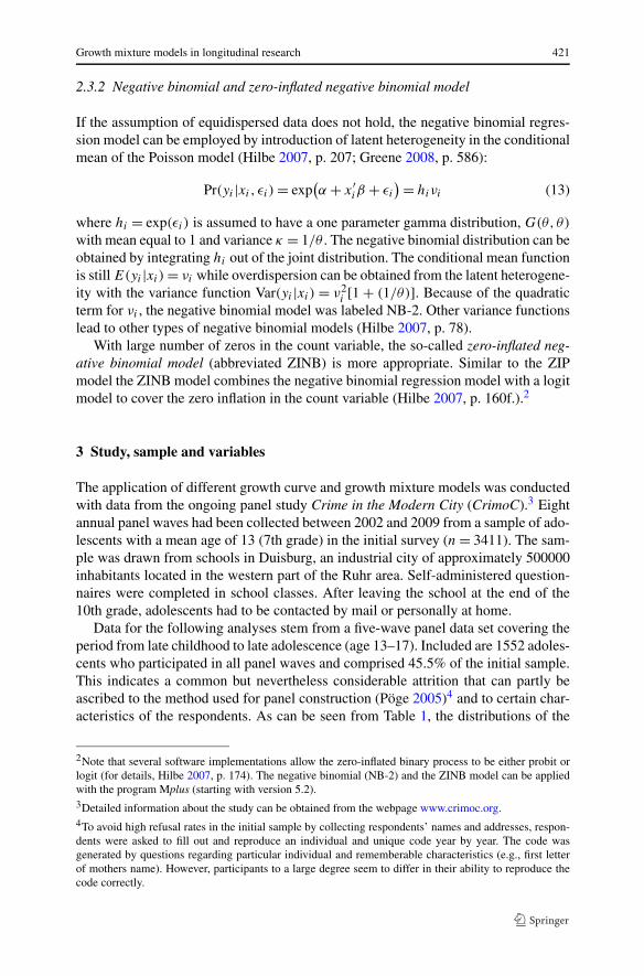
Several applications of growth mixture models with data from this investigationand a previous pilot study have been published Reinecke (2006a, 2006b, 2007, 2008).While these analyses were focused on the annual summed prevalence rates, i.e. theversatility of adolescents delinquent behavior, the current analyses are focused on theincidence rates to directly study the development of the frequency, i.e. the intensityof delinquent behavior. The annual incidence rate is a composite measure of self-reported delinquency. Respondents were as asked to give the number of delinquentbehaviors committed during the last 12 months for 16 different offenses separately.The offenses were theft of and out of cars, theft out of a vending machine, theft ofbicycles, other thefts, burglary, shoplifting, fencing, robbery, purse snatching, assaultwith and assault without a weapon, graffiti, scratching, damage to property and drugdealing. The overall annual incidence rate is given as the sum of the rates for the 16behaviors. Table 2 contains descriptive information about the annual composite mea-sures of self-reported delinquency. After a peak at age 14 (t2) the mean frequency ofdelinquent activity is constantly declining. The distributions are characterized by rel-


atively high proportions of persons who do not report any delinquent activity (% ze-ros) and relatively few persons with extreme values. Large variances, skewness andkurtosis are further characteristics which are typical for behavioral data relying onrare events. Thus, the measures of annual self-reported delinquency can be treated asoverdispersed count data with an inflation of zeros.

The following analyses are divided into three parts: first, techniques of latentgrowth curve models will be used to specify the observed outcome as a functionof time (respective age) alone and to check for potential variations around the growthfactors means. Second, latent class growth and growth mixture model specificationswill be applied to the data. Furthermore, the best fitting solutions two alternative mod-eling approaches (zero-inflated Poisson and zero-inflated negative binomial) will becompared with regard to the differences and similarities of assigning individuals tolatent classes. Third, the best growth mixture model will be enlarged by adding co-variates in order to give auxiliary information for a more precise classification and toincorporate potential predictors of the particular latent class distributions.

4 Latent growth models

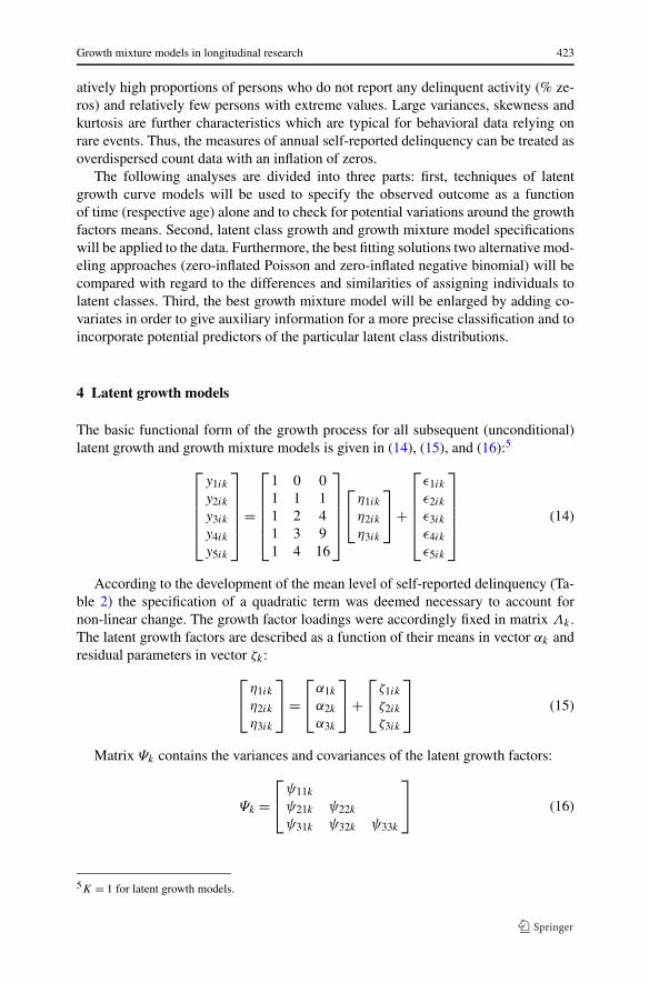
The basic functional form of the growth process for all subsequent (unconditional)latent growth and growth mixture models is given in (14), (15), and (16):5

⎡⎢⎢⎢⎢⎣

y1ik

y2ik

y3ik

y4ik

y5ik

⎤⎥⎥⎥⎥⎦ =

⎡⎢⎢⎢⎢⎣

1 0 01 1 11 2 41 3 91 4 16

⎤⎥⎥⎥⎥⎦

⎡⎣η1ik

η2ik

η3ik

⎤⎦ +

⎡⎢⎢⎢⎢⎣

ε1ik

ε2ik

ε3ik

ε4ik

ε5ik

⎤⎥⎥⎥⎥⎦ (14)

According to the development of the mean level of self-reported delinquency (Ta-ble 2) the specification of a quadratic term was deemed necessary to account fornon-linear change. The growth factor loadings were accordingly fixed in matrix Λk .The latent growth factors are described as a function of their means in vector αk andresidual parameters in vector ζk :

⎡⎣η1ik

η2ik

η3ik

⎤⎦ =

⎡⎣α1k

α2k

α3k

⎤⎦ +

⎡⎣ζ1ik

ζ2ik

ζ3ik

⎤⎦ (15)

Matrix Ψk contains the variances and covariances of the latent growth factors:

Ψk =⎡⎣ψ11k

ψ21k ψ22k

ψ31k ψ32k ψ33k

⎤⎦ (16)

5K = 1 for latent growth models.


Table 3 Comparison of different latent growth model specifications

Model Random effects Parameters Log-likelihood BIC

ZIP1 – 6 −39092.919 78229.921

ZIP2 I 7 −23596.340 47244.112

ZIP3 IS 9 −17714.575 35495.276

ZIP4 ISQ 12 −16007.225 32102.617

ZINB1 – 11 −10924.769 21930.358

ZINB2 I 12 −10206.846 20501.860

ZINB3 IS 14 −10164.167 20431.195

ZINB4 ISQ 17 −10156.666 20438.237

I = intercept; S = linear slope; Q = quadratic slope

Table 4 Estimated random effects for ZINB models

ZINB2 ZINB3 ZINB4

Parameter Est. (z-value) Est. (z-value) Est. (z-value)

ψI 8.522 (18.645) 9.423 (12.434) 6.687 (10.009)

ψS – – 0.551 (7.044) 2.491 (5.496)

ψQ – – – – 0.160 (4.796)

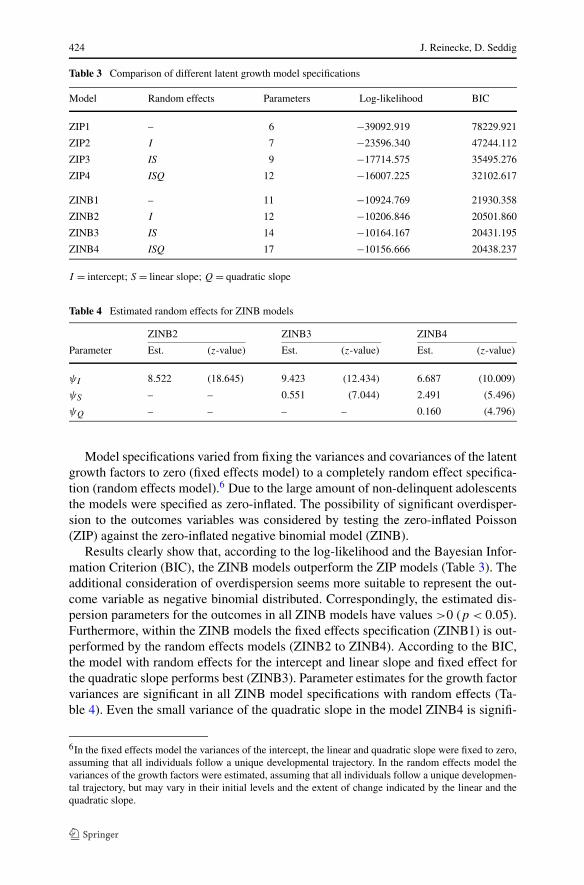
Model specifications varied from fixing the variances and covariances of the latentgrowth factors to zero (fixed effects model) to a completely random effect specifica-tion (random effects model).6 Due to the large amount of non-delinquent adolescentsthe models were specified as zero-inflated. The possibility of significant overdisper-sion to the outcomes variables was considered by testing the zero-inflated Poisson(ZIP) against the zero-inflated negative binomial model (ZINB).

Results clearly show that, according to the log-likelihood and the Bayesian Infor-mation Criterion (BIC), the ZINB models outperform the ZIP models (Table 3). Theadditional consideration of overdispersion seems more suitable to represent the out-come variable as negative binomial distributed. Correspondingly, the estimated dis-persion parameters for the outcomes in all ZINB models have values >0 (p < 0.05).Furthermore, within the ZINB models the fixed effects specification (ZINB1) is out-performed by the random effects models (ZINB2 to ZINB4). According to the BIC,the model with random effects for the intercept and linear slope and fixed effect forthe quadratic slope performs best (ZINB3). Parameter estimates for the growth factorvariances are significant in all ZINB model specifications with random effects (Ta-ble 4). Even the small variance of the quadratic slope in the model ZINB4 is signifi-

6In the fixed effects model the variances of the intercept, the linear and quadratic slope were fixed to zero,assuming that all individuals follow a unique developmental trajectory. In the random effects model thevariances of the growth factors were estimated, assuming that all individuals follow a unique developmen-tal trajectory, but may vary in their initial levels and the extent of change indicated by the linear and thequadratic slope.


Table 5 Comparison of latent class growth models (ZINB)

Model Classes Parameters Log-likelihood BIC

LCGA (ZINB) 2 15 −10326.262 20762.734

LCGA (ZINB) 3 19 −10169.237 20478.073

LCGA (ZINB) 4 23 −10142.068 20453.123

LCGA (ZINB) 5 27 −10116.018 20430.414

LCGA (ZINB) 6 31 −10098.193 20424.152

LCGA (ZINB) 7 35 −10087.260 20431.676

LCGA (ZINB) 8 39 −10076.222 20438.989

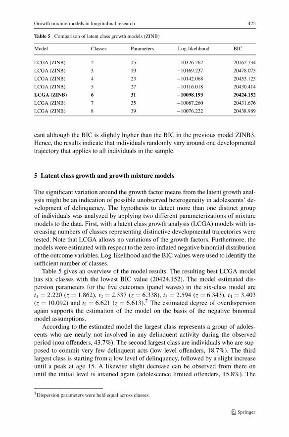
cant although the BIC is slightly higher than the BIC in the previous model ZINB3.Hence, the results indicate that individuals randomly vary around one developmentaltrajectory that applies to all individuals in the sample.

5 Latent class growth and growth mixture models

The significant variation around the growth factor means from the latent growth anal-ysis might be an indication of possible unobserved heterogeneity in adolescents’ de-velopment of delinquency. The hypothesis to detect more than one distinct groupof individuals was analyzed by applying two different parameterizations of mixturemodels to the data. First, with a latent class growth analysis (LCGA) models with in-creasing numbers of classes representing distinctive developmental trajectories weretested. Note that LCGA allows no variations of the growth factors. Furthermore, themodels were estimated with respect to the zero-inflated negative binomial distributionof the outcome variables. Log-likelihood and the BIC values were used to identify thesufficient number of classes.

Table 5 gives an overview of the model results. The resulting best LCGA modelhas six classes with the lowest BIC value (20424.152). The model estimated dis-persion parameters for the five outcomes (panel waves) in the six-class model aret1 = 2.220 (z = 1.862), t2 = 2.337 (z = 6.338), t3 = 2.594 (z = 6.343), t4 = 3.403(z = 10.092) and t5 = 6.621 (z = 6.613).7 The estimated degree of overdispersionagain supports the estimation of the model on the basis of the negative binomialmodel assumptions.

According to the estimated model the largest class represents a group of adoles-cents who are nearly not involved in any delinquent activity during the observedperiod (non offenders, 43.7%). The second largest class are individuals who are sup-posed to commit very few delinquent acts (low level offenders, 18.7%). The thirdlargest class is starting from a low level of delinquency, followed by a slight increaseuntil a peak at age 15. A likewise slight decrease can be observed from there onuntil the initial level is attained again (adolescence limited offenders, 15.8%). The

7Dispersion parameters were held equal across classes.


Table 6 Estimated means and residuals for the six-class LCGA model

Class t1 t2 t3 t4 t5

Non offenders Est. means 0.025 0.009 0.006 0.008 0.022

Residuals 0.000 0.001 0.000 0.000 0.000

Low level Est. means 0.751 0.758 0.564 0.380 0.231

Residuals −0.033 0.063 −0.008 −0.042 0.024

Adolescence Est. means 2.160 5.490 7.002 5.494 2.652

limited Residuals −0.012 −0.157 0.730 −0.780 0.249

High level/ Est. means 19.287 37.139 42.860 36.344 22.645

persistent Residuals −2.123 9.269 −5.701 −4.751 4.135

Late starters Est. means 0.027 0.123 0.523 2.497 13.380

Residuals −0.002 −0.004 0.055 −0.263 0.894

Early decliners Est. means 8.123 9.209 0.856 0.008 0.000

Residuals −0.097 0.006 −0.001 0.000 0.000

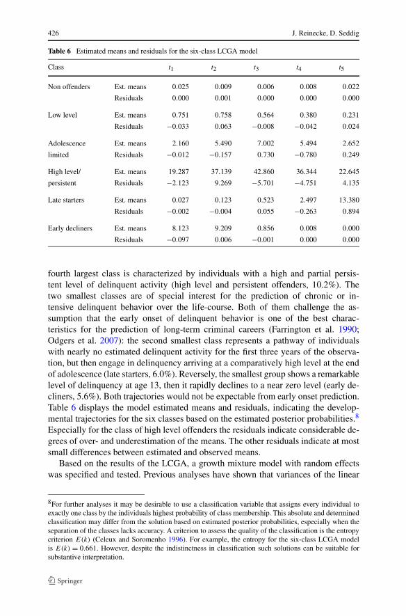
fourth largest class is characterized by individuals with a high and partial persis-tent level of delinquent activity (high level and persistent offenders, 10.2%). Thetwo smallest classes are of special interest for the prediction of chronic or in-tensive delinquent behavior over the life-course. Both of them challenge the as-sumption that the early onset of delinquent behavior is one of the best charac-teristics for the prediction of long-term criminal careers (Farrington et al. 1990;Odgers et al. 2007): the second smallest class represents a pathway of individualswith nearly no estimated delinquent activity for the first three years of the observa-tion, but then engage in delinquency arriving at a comparatively high level at the endof adolescence (late starters, 6.0%). Reversely, the smallest group shows a remarkablelevel of delinquency at age 13, then it rapidly declines to a near zero level (early de-cliners, 5.6%). Both trajectories would not be expectable from early onset prediction.Table 6 displays the model estimated means and residuals, indicating the develop-mental trajectories for the six classes based on the estimated posterior probabilities.8

Especially for the class of high level offenders the residuals indicate considerable de-grees of over- and underestimation of the means. The other residuals indicate at mostsmall differences between estimated and observed means.

Based on the results of the LCGA, a growth mixture model with random effectswas specified and tested. Previous analyses have shown that variances of the linear

8For further analyses it may be desirable to use a classification variable that assigns every individual toexactly one class by the individuals highest probability of class membership. This absolute and determinedclassification may differ from the solution based on estimated posterior probabilities, especially when theseparation of the classes lacks accuracy. A criterion to assess the quality of the classification is the entropycriterion E(k) (Celeux and Soromenho 1996). For example, the entropy for the six-class LCGA modelis E(k) = 0.661. However, despite the indistinctness in classification such solutions can be suitable forsubstantive interpretation.


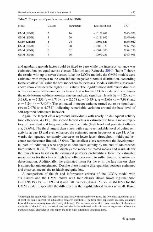
Table 7 Comparison of growth mixture models (ZINB)

Model Classes Parameters Log-likelihood BIC

GMM (ZINB) 2 16 −10158.691 20434.938

GMM (ZINB) 3 20 −10121.995 20390.936

GMM (ZINB) 4 24 −10093.843 20364.022

GMM (ZINB) 5 28 −10083.137 20371.998

GMM (ZINB) 6 32 −10074.556 20384.226

GMM (ZINB) 7 36 −10070.231 20404.965

and quadratic growth factor could be fixed to zero while the intercept variance wasestimated but set equal across classes (Mariotti and Reinecke 2010). Table 7 showsthe results with up to seven classes. Like the LCGA models, the GMM models wereestimated with respect to the zero-inflated negative binomial distribution. Accordingto the smallest BIC value the best model has four classes. Models with five classes andabove show considerable higher BIC values. The log-likelihood differences diminishwith an increase of the number of classes. Just as for the LCGA model with six classesthe model estimated dispersion parameters indicate significant levels (t1 = 3.250 (z =3.385), t2 = 2.253 (z = 9.710), t3 = 2.558 (z = 10.334), t4 = 2.668 (z = 7.998) andt5 = 5.244 (z = 7.406)). The estimated intercept variance turned out to be significant(ψI = 2.076 (z = 4.732)) indicating remarkable variation around the base level ofself-reported delinquent behavior.

Again, the largest class represents individuals with nearly no delinquent activity(non offenders, 43.1%). The second largest class is estimated to have a mean trajec-tory of persistent and frequent delinquent activity (high level and persistent offend-ers, 28.6%). The third largest class starts with a quite remarkable level of delinquentactivity at age 13 and even enhances the estimated mean frequency at age 14. After-wards, delinquency constantly decreases to lower levels throughout middle adoles-cence (adolescence limited, 18.0%). The smallest class represents the developmen-tal path of individuals who engage in delinquent activity by the end of adolescence(late starters, 8.7%).9 Table 8 displays the model estimated means and residuals forthe four classes based on the estimated posterior probabilities. Here, the estimatedmean values for the class of high level offenders seem to suffer from substantive un-derestimation. Additionally, the estimated mean for the t5 in the late starters classis somewhat underestimated. Despite these notable discrepancies between estimatedand observed means the residuals are quite low.

A comparison of the fit and information criteria of the LCGA model withsix classes and the GMM model with four classes shows lower log-likelihood(−10098.193 vs. −10093.843) and BIC values (20424.152 vs. 20364.022) for theGMM model. Especially the difference in the log-likelihood values is small. Based

9Although the model with four classes is statistically the favorable solution, the five-class model can be ofat least the same interest for substantive research questions. The fifth class represents an early withdrawfrom delinquent activity (so-called early deliners). The decision about the correct number of classes onthe basis of the BIC is a statistical one and should be reflected with substantive arguments. Given themethodological character of this paper, the four-class solution is discussed here.


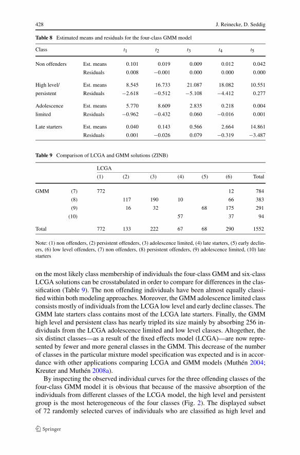
Table 8 Estimated means and residuals for the four-class GMM model

Class t1 t2 t3 t4 t5

Non offenders Est. means 0.101 0.019 0.009 0.012 0.042

Residuals 0.008 −0.001 0.000 0.000 0.000

High level/ Est. means 8.545 16.733 21.087 18.082 10.551

persistent Residuals −2.618 −0.512 −5.108 −4.412 0.277

Adolescence Est. means 5.770 8.609 2.835 0.218 0.004

limited Residuals −0.962 −0.432 0.060 −0.016 0.001

Late starters Est. means 0.040 0.143 0.566 2.664 14.861

Residuals 0.001 −0.026 0.079 −0.319 −3.487

Table 9 Comparison of LCGA and GMM solutions (ZINB)

LCGA

(1) (2) (3) (4) (5) (6) Total

GMM (7) 772 12 784

(8) 117 190 10 66 383

(9) 16 32 68 175 291

(10) 57 37 94

Total 772 133 222 67 68 290 1552

Note: (1) non offenders, (2) persistent offenders, (3) adolescence limited, (4) late starters, (5) early declin-ers, (6) low level offenders, (7) non offenders, (8) persistent offenders, (9) adolescence limited, (10) latestarters

on the most likely class membership of individuals the four-class GMM and six-classLCGA solutions can be crosstabulated in order to compare for differences in the clas-sification (Table 9). The non offending individuals have been almost equally classi-fied within both modeling approaches. Moreover, the GMM adolescence limited classconsists mostly of individuals from the LCGA low level and early decline classes. TheGMM late starters class contains most of the LCGA late starters. Finally, the GMMhigh level and persistent class has nearly tripled its size mainly by absorbing 256 in-dividuals from the LCGA adolescence limited and low level classes. Altogether, thesix distinct classes—as a result of the fixed effects model (LCGA)—are now repre-sented by fewer and more general classes in the GMM. This decrease of the numberof classes in the particular mixture model specification was expected and is in accor-dance with other applications comparing LCGA and GMM models (Muthén 2004;Kreuter and Muthén 2008a).

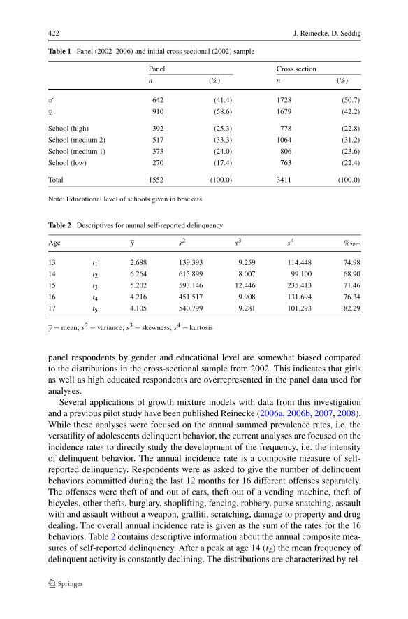
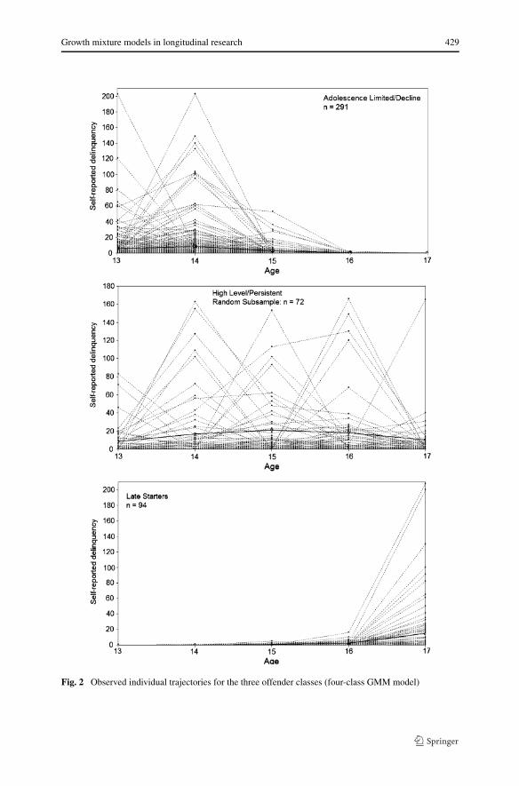
By inspecting the observed individual curves for the three offending classes of thefour-class GMM model it is obvious that because of the massive absorption of theindividuals from different classes of the LCGA model, the high level and persistentgroup is the most heterogeneous of the four classes (Fig. 2). The displayed subsetof 72 randomly selected curves of individuals who are classified as high level and


Fig. 2 Observed individual trajectories for the three offender classes (four-class GMM model)


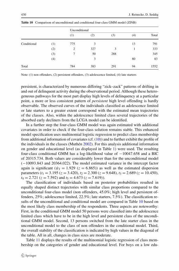
Table 10 Comparison of unconditional and conditional four-class GMM model (ZINB)

Unconditional

(1) (2) (3) (4) Total

Conditional (1) 775 3 13 791

(2) 2 327 3 1 333

(3) 7 50 288 345

(4) 3 80 83

Total 784 383 291 94 1552

Note: (1) non offenders, (2) persistent offenders, (3) adolescence limited, (4) late starters

persistent, is characterized by numerous differing “zick–zack” patterns of drifting inand out of delinquent activity during the observational period. Although these hetero-geneous pathways for the most part display high levels of delinquency at a particularpoint, a more or less consistent pattern of persistent high level offending is hardlyobservable. The observed curves of the individuals classified as adolescence limitedor late starters to a greater extent correspond with the estimated mean trajectoriesof the classes. Also, within the adolescence limited class several trajectories of theabsorbed early decliners from the LCGA model can be identified.

In a further step the four-class GMM model was again estimated with additionalcovariates in order to check if the four-class solution remains stable. This enhancedmodel specification uses multinomial logistic regression to predict class membershipfrom additional information of covariates (cf. (10)) and to further exhibit the profile ofthe individuals in the classes (Muthén 2002). For this analysis additional informationon gender and educational level (as displayed in Table 1) were used. The resultingfour-class conditional GMM has a log-likelihood value of −10047.658 and a BICof 20315.734. Both values are considerably lower than for the unconditional model(−10093.843 and 20364.022). The model estimated variance in the intercept factoragain is significant (ψI = 1.929 (z = 6.865)) as well as the estimated dispersionparameters (t1 = 3.195 (z = 3.420), t2 = 2.300 (z = 9.648), t3 = 2.689 (z = 10.450),t4 = 2.721 (z = 7.592) and t5 = 4.673 (z = 7.619)).

The classification of individuals based on posterior probabilities resulted inequally shaped distinct trajectories with similar class proportions compared to theunconditional four-class model (non offenders, 45.0%; high level and persistent of-fenders, 25%; adolescence limited, 22.5%; late starters, 7.5%). The classification re-sults of the unconditional and conditional model are compared in Table 10 based onthe most likely class membership of the respondents. Three aspects are noteworthy:First, in the conditional GMM model 50 persons were classified into the adolescencelimited class which have to be in the high level and persistent class of the uncondi-tional GMM model. Second, 13 persons switched from the late starter class in theunconditional model to the class of non offenders in the conditional model. Third,the overall stability of the classification is indicated by high values in the diagonal ofthe table. All in all, changes in class sizes are moderate.

Table 11 displays the results of the multinomial logistic regression of class mem-bership on the categories of gender and educational level. For boys on a low edu-


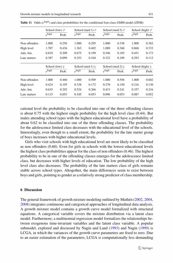
Table 11 Odds (elogit) and class probabilities for the conditional four-class GMM model (ZINB)

School (low) � School (med 1) � School (med 2) � School (high) �elogit Prob. elogit Prob. elogit Prob. elogit Prob.

Non offenders 1.000 0.256 1.000 0.295 1.000 0.338 1.000 0.382

High level 1.707 0.436 1.363 0.402 1.089 0.368 0.868 0.333

Ado. lim. 0.818 0.209 0.675 0.199 0.546 0.185 0.451 0.173

Late starters 0.387 0.099 0.353 0.104 0.322 0.109 0.293 0.112

School (low) � School (med 1) � School (med 2) � School (high) �elogit Prob. elogit Prob. elogit Prob. elogit Prob.

Non offenders 1.000 0.460 1.000 0.509 1.000 0.556 1.000 0.602

High level 0.424 0.195 0.338 0.172 0.270 0.150 0.216 0.130

Ado. lim. 0.635 0.292 0.524 0.266 0.433 0.241 0.357 0.216

Late starters 0.115 0.053 0.105 0.053 0.096 0.053 0.087 0.052

cational level the probability to be classified into one of the three offending classesis about 0.75 with the highest single probability for the high level class (0.44). Butmales attending school types with the highest educational level have a probability ofabout 0.62 to be classified into one of the three offending classes. The probabilityfor the adolescence limited class decreases with the educational level of the schools.Interestingly, even though to a small extent, the probability for the late starter groupof boys increases with higher educational levels.

Girls who visit schools with high educational level are most likely to be classifiedas non offenders (0.60). Even for girls in schools with the lowest educational levelsthe highest class probabilities appear for the class of non offenders (0.46). The highestprobability to be in one of the offending classes emerges for the adolescence limitedclass, but decreases with higher levels of education. The low probability of the highlevel class also decreases. The probability of the late starters class of girls remainsstable across school types. Altogether, the main differences seem to exist betweenboys and girls, pointing to gender as a relatively strong predictor of class membership.

6 Discussion

The general framework of growth mixture modeling outlined by Muthén (2002, 2004,2008) integrates continuous and categorical approaches of longitudinal data analysis.A growth mixture model contains a growth curve model formalized with structuralequations. A categorical variable covers the mixture distribution via a latent classmodel. Furthermore, a multinomial regression model formalizes the relationships be-tween exogenous time-invariant variables and the latent class variable. A popularsubmodel, explored and discussed by Nagin and Land (1993) and Nagin (1999) isLCGA, in which the variances of the growth curve parameters are fixed to zero. Dueto an easier estimation of the parameters, LCGA is computationally less demanding


and thus useful for a first evaluation of the unobserved heterogeneity of the data. Ifcount data with large amounts of zeros are analyzed, the outcome variables can beassumed as zero-inflated Poisson or zero-inflated negative binomial distributed. Thelatter one considers highly overdispersed distributions.

Data from a five-wave panel study of adolescents have been used to study unob-served heterogeneity in the development of deviant and delinquent behavior. In a firststep the outcome variable has been analyzed by means of a latent quadratic growthmodel under zero-inflated Poisson and zero-inflated negative binomial specifications.Due to the overdispersed data, model variants with the negative binomial specificationhave always better model fits compared to those ones assuming Poisson distributions.

With latent class growth analysis (LCGA) models up to eight classes have beentested. According to the BIC, the model with six classes performed best. All classescan be interpreted substantially. But LCGA treats the growth curve variables as fixedeffects and thus does not account for possible variation within the classes. Possibleoverlaps of individual trajectories from different classes are therefore ignored.

Within GMM the variance of the intercept was estimated for models up to sevenclasses. According to the BIC, the model with four classes performed best. Simi-lar to analyses of Muthén (2004) and Kreuter and Muthén (2008a) GMM results inless classes than LCGA. The consideration of possible overlaps in trajectories leadsto a better substantive interpretation of the development of delinquency. Additionalvariations of the linear slope and the quadratic slope did not result in further modelimprovements albeit model estimations problems increased with additional parame-ters to be estimated.

Decisions about the correct number of classes in growth mixture models can alsoinvolve a likelihood ratio-based method for testing k − 1 classes against k classesdeveloped by Lo et al. (2001) (LMR-LRT) or the bootstrapped likelihood ratio test(BLRT) proposed by McLachlan and Peel (2000). The performance of these tests fornon normal outcomes is unclear (Jeffries 2003) and the implications for applicationshas not been discussed yet.

A next step in analysis could be to test a non-parametric specification of the growthmixture model (Kreuter and Muthén 2008a, 2008b; Muthén and Asparouhov 2008).While the basic GMM assumes a specific (normal) distribution for the random effects,the non-parametric version does not make any such assumption. However, a firstinspection of the individual intercept factor scores for the three offender classes fromthe four-class GMM model presented in this paper provided no clear evidence for anon-normally distributed variation around the estimated intercept.

References

Boers, K., Reinecke, J., Seddig, D., Mariotti, L.: Explaining the development of adolescent violent delin-quency. Eur. J. Criminol. 7, 499–520 (2010)

Celeux, G., Soromenho, G.: An entropy criterion for assessing the number of clusters in a mixture model.J. Classif. 13, 195–212 (1996)

Curran, P.J., Muthén, B.: The application of latent curve analysis to testing developmental theories inintervention research. Am. J. Community Psychol. 27, 567–595 (1999)

Dempster, A.P., Laird, N.M., Rubin, D.B.: Maximum likelihood from incomplete data via the EM algo-rithm. J. R. Stat. Soc. B 39(1), 1–38 (1977)


Duncan, T.E., Duncan, S.C., Strycker, L.A.: An Introduction to Latent Variable Growth Curve Modeling.Concepts, Issues and Applications, 2nd edn. Lawrence Earlbaum, Mahwah (2006)

Farrington, D.P., Loeber, R., Elliott, D.S.: Advancing knowledge about the onset of delinquency and crime.In: Lahey, B., Kazdin, A. (eds.) Advances in Clinical Child Psychology, vol. 13, pp. 283–342. PlenumPress, New York (1990)

Greene, W.: Functional forms for the negative binomial model for count data. Econ. Lett. 99, 585–590(2008)

Hilbe, J.M.: Negative binomial regression. Cambridge University Press, Cambridge (2007)Jeffries, N.O.: A note on testing the number of components in a normal mixture. Biometrika 90, 991–994

(2003)Kreuter, F., Muthén, B.: Analyzing criminal trajectory profiles: bridging multilevel and group-based ap-

proaches using growth mixture modeling. J. Quant. Criminol. 24, 1–31 (2008a)Kreuter, F., Muthén, B.: Longitudinal modeling of population heterogeneity: methodological challenges

to the analysis of empirically derived criminal trajectory profiles. In: Hancock, G.R., Samuelsen,K.M. (eds.) Advances in Latent Variable Mixture, Modeling, pp. 53–75. Information Age Publishing,Charlotte (2008b)

Lambert, D.: Zero-inflated Poisson regression with an application to defects in manufacturing. Techno-metrics 34, 1–13 (1992)

Lo, Y., Mendell, N.R., Rubin, D.B.: Testing the number of components in a normal mixture. Biometrika88(3), 767–778 (2001)

Mariotti, L., Reinecke, J.: Wachstums- und Mischverteilungsmodelle unter Berücksichtigung un-beobachteter Heterogenit: Empirische Analysen zum delinquenten Verhalten Jugendlicher in Duis-burg. Institut für sozialwissenschaftliche Forschung e.V., Münster (2010)

McArdle, J.J.: Dynamic but structural equation modeling of repeated measures data. In: Nesselroade,J.R., Cattell, R.B. (eds.) Handbook of Multivariate Experimental Psychology, 2nd edn., pp. 561–614.Plenum, New York (1988)

McArdle, J.J., Epstein, D.: Latent growth curves within developmental structural equation models. ChildDev. 58, 110–133 (1987)

McLachlan, G., Peel, D.: Finite Mixture Models. Wiley, New York (2000)Meredith, M., Tisak, J.: Latent curve analysis. Psychometrika 55(1), 107–122 (1990)Muthén, B.: Analysis of longitudinal data using latent variable models with varying parameters. In: Collins,

L.M., Horn, J.L. (eds.) Best Methods for the Analysis of Change: Recent Advances, UnansweredQuestions, Future Directions, pp. 1–17. APA, Washington (1991)

Muthén, B.: Latent variable modeling with longitudinal and multilevel data. Sociol. Method. 27, 453–480(1997)

Muthén, B.: Latent variable mixture modeling. In: Marcouldies, G.A., Schumacker, R.E. (eds.) New De-velopments and Techniques in Structural Equation Modeling, pp. 1–33. Lawrance Erlbaum, Mahaw(2001a)

Muthén, B.: Second-generation structural equation modeling with a combination of categorical and con-tinuous latent variables: new opportunities for latent class/latent growth modeling. In: Collins, L.,Sayer, A. (eds.) New Methods for the Analysis of Change, pp. 291–322. APA, Washington (2001b)

Muthén, B.: Beyond SEM: general latent variable modeling. Behaviormetrika 29(1), 81–117 (2002)Muthén, B.: Statistical and substantive checking in growth mixture modeling: comment on Bauer and

Curran (2003). Psychol. Methods 8, 369–377 (2003)Muthén, B.: Latent variable analysis: growth mixture modeling and related techniques for longitudinal

data. In: Kaplan, D. (ed.) The SAGE Handbook of Quantitative Methodology for the Social Sciences,pp. 345–368. Sage, Thousand Oaks (2004)

Muthén, B.: Latent variable hybrids: overview of old and new models. In: Hancock, G.R., Samuelsen,K.M. (eds.) Advances in Latent Variable Mixture Models, pp. 1–24. Information Age Publishing,Charlotte (2008)

Muthén, B., Asparouhov, T.: Growth mixture modeling: analysis with non-Gaussian random effects. In:Fitzmaurice, G., Davidian, M., Verbeke, G., Molenberghs, G. (eds.) Longitudinal Data Analysis,pp. 143–165. Chapman & Hall/CRC Press, Boca Raton (2008)

Muthén, B., Muthén, L.: Integrating person-centered and variable-centered analysis: growth mixture mod-eling with latent trajectory classes. Alcohol. Clin. Exp. Res. 24(6), 882–891 (2000a)

Muthén, B., Muthén, L.: The development of heavy drinking and alcohol-related problems from ages 18to 37 in a U.S. national sample. Journal of Studies on Alcohol 61, 290–300 (2000b)

Muthén, L., Muthén, B.: Mplus User’s Guide, 4th edn. Muthén & Muthén, Los Angeles (2006)


Muthén, L., Muthén, B.: Mplus User’s Guide, 6th edn. Muthén & Muthén, Los Angeles (2010)Muthén, B., Shedden, K.: Finite mixture modeling with mixture outcomes using the EM algorithm. Bio-

metrics 55(2), 463–469 (1999)Nagin, D.S.: Analyzing developmental trajectories: a semi-parametric, group-based approach. Psychol.

Methods 4, 139–157 (1999)Nagin, D.S.: Group-Based Modeling of Development. Harvard University Press, Cambridge (2005)Nagin, D.S., Land, K.C.: Age criminal careers, and population heterogeneity: specification and estimation

of a nonparametric, mixed Poisson model. Criminology 31(3), 327–362 (1993)Nylund, K., Asparouhov, T., Muthén, B.O.: Deciding on the number of classes in latent class analysis and

growth mixture modeling. A Monte Carlo simulation study. Struct. Eq. Model. 14, 535–569 (2007)Odgers, C.L., Caspi, A., Poulton, R., Harrington, H., Thompson, M., Broadbent, J.M., Dickson, N., Sears,

M.R., Hancox, B., Moffit, T.E.: Prediction of adult health burden by conduct problem subtypes inmales. Arch. Gen. Psychiatry 64, 476–484 (2007)

Pöge, A.: Persönliche Codes bei Längsschnittstudien: Ein Erfahrungsbericht. ZA-Inf. 56, 50–69 (2005)Rao, C.R.: Some statistical methods for comparison of growth curves. Biometrics 14, 1–17 (1958)Reinecke, J.: Delinquenzverläufe im Jugendalter: Empirische Überprüfung von Wachstums- und Mis-

chverteilungsmodellen. Institut für sozialwissenschaftliche Forschung e.V., Münster (2006a)Reinecke, J.: Longitudinal analysis of adolescents’ deviant and delinquent behavior. Applications of latent

class growth curves and growth mixture models. Methodology 2, 100–112 (2006b)Reinecke, J.: The development of deviant and delinquent behavior of adolescents. Applications of latent

class growth curves and growth mixture models. In: van Montfort, K., Oud, J., Satorra, A. (eds.) Lon-gitudinal Models in the Behavioral and Related Sciences, pp. 239–266. Lawrence Erlbaum, Mahwah(2007)

Reinecke, J.: Klassifikation von Delinquenzverläufen: Eine Anwendung von Mischverteilungsmodellen.In: Reinecke, J., Tarnai, C. (eds.) Klassifikationsanalysen in Theorie und Praxis, pp. 189–218. Wax-mann, Münster (2008)

Roeder, K., Lynch, K.G., Nagin, D.S.: Modeling uncertainty in latent class membership: a case study incriminology. J. Am. Stat. Assoc. 94, 766–776 (1999)

Ross, S.M.: Introduction to Probability Models, 5th edn. Academic Press, New York (1993)Rost, J., Langeheine, R.: Applications of Latent Trait and Latent Class Models in the Social Sciences.

Waxmann, Münster (1997)Schwarz, G.: Estimating the dimension of a model. Ann. Stat. 6(2), 461–464 (1978)Tucker, L.R.: Determination of parameters of a functional relation by factor analysis. Psychometrika 23,

19–23 (1958)Willet, J.B., Sayer, A.G.: Using covariance structure analysis to detect correlates and predictors of indi-

vidual change over time. Psychol. Bull. 116(2), 363–381 (1994)

Growth mixture models in longitudinal research · Growth mixture models in longitudinal research...

Documents

Transcript of Growth mixture models in longitudinal research · Growth mixture models in longitudinal research...