Working Paper 05-41(04) Dpto. de Historia Económica e Instituciones Economic History and Institutions Series 04 Universidad Carlos III de Madrid June 2005 Calle Madrid 126, 28903 Getafe (Spain)

GROWTH, INEQUALITY, AND POVERTY IN LATIN AMERICA:

HISTORICAL EVIDENCE, CONTROLLED CONJECTURES∗

Leandro Prados de la Escosura+ Abstract_______________________________________________________________

How have growth and inequality affected poverty reduction in Latin America over the long run? On the basis of the available evidence on growth and inequality tentative answers and conjectures are proposed about the long run evolution of poverty in Latin America. Modern Latin America experienced sustained growth since mid nineteenth century only brought to a halt during the 1980s. Inequality, in turn, rose steadily until a high plateau in which it has stabilized over the last four decades of the twentieth century. A calibration exercise on the basis of López and Servén (2005) recent empirical research suggests that absolute poverty has experienced a long-run decline in Latin America since the late nineteenth century, interrupted in the 1890s and the 1930s, and only reversed in the 1980s. Growth emerges as the main element underlying the reduction in absolute poverty, and almost exclusively in the second half of the twentieth century. JEL classification: N16, N36, I32 http://www.uc3m.es/uc3m/dpto/HISEC/Doctrab/2005/wp05-41(04).pdf Keywords: Growth, inequality, poverty, Latin America

∗ This paper is the result of a short-term consultancy research for a project on growth and poverty in Latin America carried out at the Latin America & the Caribbean Region Office of the World Bank. Humberto López and Luis Servén kindly allowed me access to their unpublished research on growth, inequality, and poverty. Luis Bértola shared with me his wide knowledge of Latin America’s historical inequality. I am indebted to Roberto Vélez Grajales for his excellent research assistance and to Humberto López and Patricia Macchi for their help with the calibration of poverty reduction. Comments by Pablo Astorga, Stefan Houpt, and Humberto López on an early draft are most appreciated. Observations and remarks by by participants at the Economic History Seminar of Lund University were most valuable. I am solely responsible for its errors. + Prados de la Escosura, Dpto de Historia Económica e Instituciones. Universidad Carlos III de Madrid. E-mail: leandro.prados.delaescosura@uc3m.es

Introduction

How much has Latin America grown since its colonial independence? Has her

gap with advanced countries widened steadily over time? When did she fall behind?

How has inequality evolved historically? Is today’s high inequality a permanent feature

of modern Latin America? How have growth and inequality affected poverty reduction

in the long run?.

All these are pressing questions for economists, social scientists, and historians

interested in Latin America. To provide a distinctive and definitive answer to each of

them is beyond the individual effort. In this paper I will just present an overview of how

much can be ascertained and what tentative answers can be given in the current state of

research. From the growing literature on pro-poor growth some findings are especially

relevant for my task. Poverty reduction depends both on growth of average incomes and

on how income is distributed and the extent it does is closely linked to the sensitivity of

poverty to both of them (the so called growth elasticity and inequality elasticity of

poverty). We also know that the initial levels of development and inequality condition

the impact on poverty of growth and improvements on income distribution. I will,

hence, divide the exposition into three sections, dedicated to examine long-run trends in

growth and inequality, and, on the basis of the first two sections’ findings and the

empirical current research, to calibrate poverty reduction over the long run in modern

Latin America.

Long-run growth

Unfortunately, research in quantitative economic history of Latin America has

still a long way to go and we lack complete sets of homogenously constructed GDP

estimates that would allow space and time international comparisons. Independent

recent attempts to build GDP series for Argentina, Chile, Colombia, and Uruguay only

mitigate the problem of assessing quantitatively the performance of Latin America over

time1.

This lack of hard empirical evidence has not prevented ambitious interpretations

of Latin American long-run economic performance to spread. A view that stresses a

long run relative decline since independence has been favored in the literature (see, for

example, Victor Bulmer-Thomas (1994: 410)). It is also widely accepted that the origins

1 Cf. Cortés Conde (1994, 1997) and Della Paolera et al. (2003) for Argentina; GRECO (2000) for Colombia; Díaz et al. (1998) for Chile; and Bértola (1998) for Uruguay. See Appendix A for the GDP series used here.

2

of modern Latin American retardation are located in the nineteenth century (John

Coatsworth, 1993, and Stephen Haber, 1997). Coatsworth (1998) underlines, in turn,

that Latin America fell behind between 1700 and 1900, as the gap to the US remained

unaltered over the twentieth century.

When did Latin America fall behind has important repercussions for the ongoing

debate in which ad hoc interpretations are provided for assumed periods of decline. For

example, the relevance of the interpretation that puts the burden of the explanation in

the colonial legacy is closely dependent on the fact that Latin American retardation had

taken place in the early nineteenth century. If this is not the case, the strength of the

argument weakens dramatically. In the following paragraphs a quantitative and

comparative assessment of Latin America’s performance is carried out in an attempt to

cast some light on the hot issue of when Latin America lagged behind.

A word of caution is required, however, before the quantitative results are

discussed. Dissatisfaction with international comparisons carried out on the basis of

trading exchange rate-converted GDP per head has led way to purchasing power parity

(PPP) adjusted GDP estimates. Unfortunately, the construction of PPP converters

involves high costs in terms of time and resources. An indirect method to derive

historical estimates of real income levels for a large sample of countries, popularized by

Angus Maddison (1995, 2001, 2003), is the backward projection of the PPP-adjusted

GDP per capita for a recent (usually the latest) benchmark with volume indices derived

from national accounts data. This short-cut has the presentation advantage of providing

international growth rates identical, by construction, to those calculated from national

accounts. A distant PPP benchmark introduces, nonetheless, distortions in inter-

temporal comparisons since its validity depends on how stable the basket of goods and

services used to construct the original PPP converters remains over time. Long term

growth alters the composition of output and consumption and, hence, relative prices,

rendering international comparisons of per capita income based upon remote PPPs

highly questionable (Prados de la Escosura, 2000).

Unfortunately, in order to facilitate comparisons over space and time the dearth

of data has forced me to link volume estimates computed at national relative prices to

benchmark estimates for the year 1980 expressed in 1980 Geary-Khamis dollars

available for most Latin American countries from the UN’s International Comparisons

Project (ICP IV).

3

Why to provide new, though still defective GDP series for Latin America when

both Maddison (1995, 2003) and Astorga et al. (1998, 2003a) have presented their own

estimates? There two main reasons, the first one relates to the chosen benchmark, 1980

represents a more sound choice than those for 1990 and 1970 preferred by Maddison

and Astorga et al., respectively. Neither for 1990 nor 1970 a systematic construction of

purchasing power parity exchange rates (PPP) have been constructed. Latin America

was excluded from the United Nations International Comparisons Project (ICP) Phase V

that resulted in the construction of multilateral PPPs for 56 countries. Maddison (1995,

2003) estimated GDP levels for Latin American countries in 1990, first by projecting

1980 per capita GDP levels expressed in 1980 international dollars (that resulted from

ICP’s most complete sample of LAC countries until the most recent one for 1996) with

volume indices of product per head taken from each country’s national accounts. Then,

he reflated the GDP levels for 1990 (expressed in 1980 Geary-Khamis dollars) with the

U.S. implicit GDP deflator in order to obtain output levels in 1990 international dollars.

As regards Astorga et al. (1998, 2004a, 2004b) 1970 benchmark, expressed in

international dollars, originally published by CEPAL [the Spanish acronym of ECLA]

(1978), were derived from nominal GDP levels provided by national accounts and PPP

exchange rates obtained by projecting directly computed PPPs for 1960 with each Latin

American country’s inflation differential with respect to the USA (CEPAL, 1978: 7-8).

The 1960 benchmark provides bilateral PPPs (Fisher PPPs is Astorga et al. choice)

directly computed by the Economic Commission for Latin America [ECLA] for 1960

(Braithwaite, 1968; ECLA, 1968)2. Among the two directly computed benchmarks

available (1960 and 1980) I chose the latter for this paper, as it provides multilateral

PPPs and its country coverage includes most OECD members3. Alternatively, Geary-

Khamis PPPs derived by the UN’s International Comparisons Project [ICP] for 1996

could have been used but the 1980 benchmark provides a less remote year for the time

span considered and it is, hence, preferable4. The second reason why my estimates differ

from the previous ones by Maddison and Astorga et al. is that I have widened the

country coverage including the latest national GDP estimates available (Appendix A). 2 The commodity basket included 261 consumption goods and 113 investment goods for capital cities in nineteen Latin American countries and the US (Houston and Los Angeles). Prices were collected in 1960/62. Quantity expenditure weights for a Latin American average and the US in 1960 were used (ECLA, 1968; Braithwaite, 1968). 3 Nonetheless, I have replicated the whole exercise presented here at 1960 international prices with no major discrepancies in the results. In another paper (Prados de la Escosura, 2004b) I rely on the 1960 benchmark expressed at US relative prices. 4 Hofman (2000, 2001) also relies on 1980 international dollars for Latin America.

4

Graph 1 and Table 1 present population-weighted measures of real GDP per

head in Latin America over one and a half centuries. Some main features of historical

performance in Latin America can be pointed. In the first place, the origins of modern

economic growth, as defined by a sustained increase in output per person, can be traced

back to, at least, mid-nineteenth century, as a sustained improvement in GDP per capita

is already observable since the 1860s. Latin America appears to have experienced a

sustained and gradual growth over more than a century only broken during the 1890s,

the Great Depression and, especially, the early 1980s crisis. In Table 1 growth rates are

presented for different groups of Latin American countries, with the lengthier the

coverage the lower the number of countries comprised. Fortunately, though, the picture

they offer of Latin America’s performance seems quite robust. After a slow start in the

mid-nineteenth century, Latin America appears to grow significantly during the

eighteen seventies and eighties and, after the slow down of the 1890s, to accelerate up

to World War I. A comparison with the group of advanced countries included under the

label OECD shows that Latin America grew faster in the periods 1870-90 (LA6) and,

especially, in the 1900-1913 (LA6 and LA10). Latin America’s output per head slowed

down its pace because of World War I and reached a halt in the years of the Great

Depression, but its comparative performance was not dissimilar from that of OECD

countries. In sum, during the first phase of sustained growth in per capita income, 1870-

1929, Latin America does not appear to have fallen behind, but to keep pace with the

advanced country club but, like everybody else, grew slower than the U.S. After the

Depression, Latin America enjoyed its fastest phase of growth that lasted more than

four decades, at a pace closer to that of OECD, in which its better performance in the

1970s made somehow for a slower growth in the so called ‘Golden Age’ (1950-73). The

1980s represent a major break in the long-run performance of Latin America that fell

short of being offset by the sluggish growth of the 1990s. Thus, while the growth of the

early phase, 1860s-1929, was superseded by the performance of the 1930s-1980, the

post-1980 era offers a phase of slowing down.

The comparison with Spain, a country that shares with Latin America culture

and institutions, is illuminating. Spain exhibits a pace of growth similar to Latin

America’s over 1870-1929 and after the 1930s crisis (magnified by the Civil War).

Spain, however, grew faster in the 1950s and experienced super-growth in the 1960s

5

and early 1970s5. Moreover, in spite of the nearly stagnation in the decade of ‘transition

to democracy’ (1975-85), Spain’s growth has been above OECD average during the last

two decades of the twentieth century.

If a neo-classical growth approach is chosen, a different view of Latin American

performance results. As Latin America started from lower levels of GDP per head and,

subsequently, poorer endowment of human and physical capital, a faster growth rate

should, ceteris paribus, be expected. Hence, her performance would appear

disappointing, especially in the second half of the twentieth century when, in an

increasingly globalized world, access to the latest technological vintage depended upon

a country’s social capability. The case of Spain and, more recently, of South East Asian

nations support this interpretation.

Decomposing per capita GDP growth using identity (I), provides a more

accurate explanation of Latin American slow down. If low case represents annual rates

of variation, per capita income growth results from adding the rates of variation of labor

productivity (output per economically active population [EAP], of the activity rate

(EAP per population ages 15 to 64, or potentially active population [PAP]), and that of

the PAP in total population.

ypc = y/eap + eap/pap + pap/population (I)

Labor productivity that, in the nineteen fifties and sixties, had overcome per

capita GDP growth making for a declining activity rate and for a higher dependency

rate (population below 15 and above 65 over PAP), lagged behind since the 1970s

(Table 1b). In the 1970s and, again, in the 1990s the increase in the activity rate, related

to the reduction of unemployment and, especially in the nineties, to the incorporation of

women to the labor force (Astorga et al., 2003: 35). Actually, with hardly any labor

productivity growth, per capita income continued rising on the basis of an increase in

the PAP/population ratio (as the demographic transition reached an end) plus the rise in

the activity rate. A further decomposition of labor productivity into physical and human

capital per worker and total factor productivity (TFP) is necessary to understand the

slowing down of workers’ efficiency. Astorga et al. (2003: 34) suggest, after 1980, an

average decline in TFP growth together with a fall in capital deepening for a six country

sample (LA4 plus Argentina and Colombia). Hofman (2001) has a more benign view of

5 In Spain, the year 1938 represents a trough in economic performance.

6

TFP growth and points that the decline in labor productivity reflects a ‘strong increase’

in labor inputs6.

So far, the focus of attention has been on Latin America as a whole but the

region conceals a heterogeneous group of countries that exhibit substantial

discrepancies in their factor endowments and long-run performance. The fact that most

economic historians only address their research to a country or just to a one of its

regions supports the case. Latin America as a whole is, however, what scholars see from

the outside and, therefore, remains a valid concept once allowance is made for the wide

dispersion in terms of performance and policies. Inequality between Latin American

countries increase during the first époque of globalization (1870-1913) as countries

reacted very differently depending on their exposition to international commodity and

factor movements (Prados de la Escosura, 2004). De-globalization in the Interwar years

witnessed a reduction in across-country inequality. Between the early forties and 1970,

across-countries inequality rose and, then, collapsed to mid-nineteenth century levels.

Such a process of convergence within Latin America is parallel to the divergence with

respect to the advanced countries as will be discussed below.

Per capita real GDP levels for major Latin American countries at roughly

decadal benchmarks are presented since 1850 in Graph 2, depending on the availability

of historical estimates. The high variance of growth rates of GDP per capita in Latin

America (Table 2) is worth highlighting. Argentina, Chile and Mexico income per head

grew above Latin America’s average between 1870 and 1913, while Brazil, Colombia,

Peru, and Venezuela did it over 1913-1938. On the whole, during the early phase of

modern economic growth (1870-1929) Colombia, Peru, Venezuela and, to lesser extent,

Argentina grew above the region’s average. In the second phase of sustained expansion

(1938-80), Mexico and especially Brazil emerge above the average, while Chile stands

alone above it in the last two decades of the twentieth century. As countries starting

from lower income levels have grown faster than average over the long run, a pattern of

convergence among Latin American nations has been building up over time.

When we look at the components of per capita GDP growth, a systematic pattern

emerges across countries (Table 3). Labor productivity growth fell behind GDP per

head growth in the last two decades of the twentieth century, but was offset by the rise

in the activity rate and by the demographic gift of an increasing share of potentially

6 Also Fajnzylber and Lederman (2000) and Hofman (2000) found a negative TFP growth in the 1980s.

7

active population. It is worth mentioning that the demographic gift takes place since

1970, in common with U.N. labeled ‘less developed countries’ (Lee, 2003) and was not

offset by a decline in the rate of activity resulting from higher unemployment (except

for Brazil in the 1990s and Mexico in the 1980s). Per capita income growth has been

sustained, in some cases, or has not fallen more sharply, in others, largely thanks to the

demographic bonus. Finally the somehow inverse evolution between the rate of activity

and labor productivity might suggest a falling capital-labor ratio due to fast growing

employment.

The comparison between Latin America and other regions or countries allow us

to place Latin America’s achievements into an international perspective. But, which is

the adequate yardstick to assess Latin America’s success or failure? Usually Latin

America is examined in the U.S. mirror and usual interpretations of early failure and

moderate success in the twentieth century derive that way. However, even western

European economies fell behind relative to the U.S. over the nineteenth century, while

the fact that Latin America’s relative position to the U.S. remained mostly unaltered

during the twentieth century seems at odds with the catching up experience in large

areas of the Periphery (Southern Europe, Southeast Asia), in which the gap with the

U.S. was significantly reduced after 1950, whereas Latin America only grew faster that

the US in the 1970s. The US represents, thus, a questionable yardstick. I propose

instead to use a more comprehensive yardstick, the group of advanced countries from

the Old and New World that are today part of the OECD, [hereafter, OECD for short].

This country sample also includes countries that belonged to the European Periphery

but are part of the Core today, such as Italy, Ireland, or Spain. Actually, Spain has been

singled out in the comparisons since she shares institutions with Latin America while

she offers a different experience of economic development.

Graph 3 presents the evolution of population-weighted averages of per capita

incomes in Latin America relative to the OECD average7. The relative position of Latin

America in terms of OECD GDP per head presents a wide inverted U-shape for all

country samples, except for LA4. In the early phase of modern economic growth (1870-

1929) Latin America maintained a stable relative position around 50 percent. Later, in

the phase of accelerating expansion, 1938-1980, Latin America experienced a paradox

of growth and retardation, falling by almost 20 percent. Lastly, the faltering

7 The number of countries included in each sample figures after the region’s name, that is, LA6 means that six countries are included in this Latin American (LA) sample.

8

performance of the last two decades of the twentieth century took Latin America to half

its relative position in 1929. When Latin America is compared with Spain, instead,

(Graph 3b), together with a relative improvement during the central years of the

twentieth century, resulting from Spain’s Civil War and autarkic aftermath, a sustained

decline is noticeable during its last three decades. It appears, then, that during the period

considered, that spans over two phases of globalization and one of de-globalization,

Latin America does not seem to have fallen behind until the late twentieth century. Such

a finding is in stark contradiction with conventional assessments that locate Latin

American retardation in the nineteenth century.

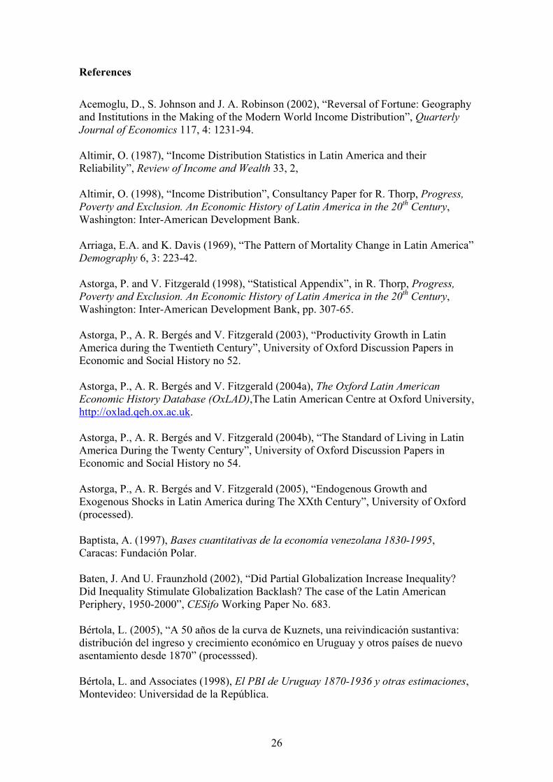
Table 4 decomposes Latin America’s position relative to OECD and to Spain in

terms of GDP per head’s components, while Table 5 replicates the exercise for major

individual countries. Lack of country coverage prevent us from extending the exercise

for Latin America as a whole before 1950 (Panel A), so a reduced exercise

decomposing GDP per head into GDP per potentially active population and the share of

population ages 15 to 64 is provided (Panel B). It can be noticed that labor productivity

systematically reaches higher relative levels than GDP per head as a consequence of a

lower population in working age, and, when the comparison is carried out with OECD,

also of a lower activity rate (a feature related to a lower female participation in the labor

force).

High dependency rates in Latin America (Graph 5), resulting from a delayed

demographic transition help explain lower levels of GDP per person and, hence, higher

poverty in Latin America. The persistence of high dependency rates in Latin America

hint to the lack of incentives to reduce fertility provided by the institutional framework

and to the weak demand of human capital that helped to bring about the demographic

transition in OECD countries (Galor, 2004), and deserves more careful research.

To sum up, modern Latin America experienced sustained growth since mid

nineteenth century only brought to a halt during the 1980s. Paradoxically, as in other

cases within the Periphery, growth was accompanied by backwardness relative to

advanced countries, in particular, during the second half of the twentieth century, and

more especially since 1980. What are the implications of such findings for the ongoing

debate on Latin America’s retardation? Contrary to a widely held view, Latin America’s

retardation, vis-à-vis OECD countries, appears to be a late twentieth century

9

phenomenon8. Moreover, the decline that probably took place in the decades after

independence seems hardly comparable to the dramatic fall in Latin America’s position

relative to the OECD in the late twentieth century. It seems plausible that in the half

century after independence Latin America grew at a slower pace than during the early

phase of globalization (1870-1913) but it can be claimed that retardation took place in

only when Latin America is compared to a small group of western countries. Thus, the

empirical findings presented here seriously challenge conventional assessments that

locate Latin American retardation in the nineteenth century and link it to geography,

initial inequality of wealth and power, colonial heritage, and post-independence political

instability and turmoil. They all certainly hindered long-run growth and a counterfactual

scenario with law and order, lower inequality, and British institutions would have cast a

higher growth rate in Latin America. However, this is not the issue at stake here. Latin

America fell behind dramatically in the late twentieth century and, particularly, since

1980. Such a result demands an explanation. Was it because of inward-looking and

interventionist policies? Was it because of poorly defined and enforced property rights?

Astorga et al. (2003) claimed that it is misleading to associate import-industrialization

strategies to faltering performance as it was during the decades in which such policies

were implemented (1937-77) that growth intensified and welfare levels improved;

conversely the neo-liberal policies, including privatizations, correspond to the post-1978

phase of economic stagnation and relative decline. Astorga et al. (2003) views remind

us that simplistic explanations of Latin American backwardness, written with the

exclusive help of theory, are doomed to failure and set the agenda for further research. I

will not attempt here, therefore, an easy answer but would like to recall that the period

of fastest growth in Latin America, that from World War II till 1980, is also the one in

which Latin America fell behind OECD countries, a fate not shared by other regions of

the Periphery, such as south-western Europe and East Asia, which were catching up to

the Core. Moreover, in the post-1980 era, neo-liberal policies were not always

accompanied by deep institutional reforms that would have drastically changed the set

of incentives received by economic agents (Taylor, 1998). Government credibility and

institutional quality and stability would have help to promote growth. Trade volatility

(both in volumes and relative prices) and interest rate shocks, it has been argued, were also

major impediments to sustained economic growth and catching up (Astorga et al., 2005).

8 Of course, only the post-1850 era is analyzed here but similar results appear when the scope is widened both in time and regional coverage. Cf. Prados de la Escosura (2004b).

10

Long-run Inequality

Latin America is today the world region in which inequality is highest, with an

average Gini coefficient above 50 during the last four decades of the twentieth century

(Deininger and Squire, 1996, 1998). A stable income distribution since the post-war

period has worsened after 1980 (Altimir, 1987; Morley, 2000). Furthermore, no

significant improvement in the relationship between income distribution and economic

growth has taken place during the last decade (Londoño and Székely, 1997) and

inequality remained high despite episodes of sustained growth (ECLAC, 2000).

Does such an assessment apply to modern Latin American history?

Unfortunately, no quantitative assessment of long-run inequality has been carried out

for Latin America, but the perception of unrelenting inequality deeply rooted in the past,

is widespread among social scientists and historians. A good example is provided by

Bourguignon and Morrisson (2002) investigation of the historical trends in world

income inequality. Lack of empirical evidence and conventional wisdom led them to

assume that no changes in income distribution had taken place in Latin America from

independence to the mid-twentieth century. Only the path-breaking work by Bértola and

his associates (2005) for Uruguay has recently provided crude estimates of income

distribution and Gini coefficients that go back to the late nineteenth century.

How has the persistence of inequality been explained? Different alternative

interpretations have been put forward. Among them, those that emphasize its colonial

roots are worth stressing. According to Engerman and Sokoloff (1997), initial inequality

of wealth, human capital and political power conditioned institutional design and,

hence, performance in Spanish America. Large scale estates, built on pre-conquest

social organization and extensive supply of native labor, established the initial levels of

inequality. In the post-independence world, elites designed institutions protecting their

privileges. In such a path-dependent framework Government policies and institutions

restricted competition and offered opportunities to select groups (Sokoloff and

Engerman, 2000).

Moreover, Acemoglu, Johnson and Robinson (2002) maintain a different

explanation for the uneven fate of former colonies. Where abundant population showed

relative affluence, ‘extractive institutions’ were established, under which most of the

population risks expropriation at the hands of the ruling elite or the government (forced

labor and tributes, often existing already in the pre-colonial era, over the locals) with

11

political power concentrated in the hands of an elite, represented the most efficient

choice for European colonizers, despite its negative effects on long-term growth. This

would be the case of the Iberian empires in the Americas, especially in its economic

centers of Peru and New Spain.

After independence, the opening up to the international economy has been

associated to a widening of income differences within and across countries. The

opening to the international economy was seen by Dependentists as a cause of

increasing inequality across and within countries, stressing the role of the terms of trade

in Latin American retardation as either they improved and shifted resources to primary

production (Hans Singer, 1950), or deteriorated and provoked immiserizing growth

(Raúl Prebisch, 1950). Neoclassical trade theory predicts, in turn, that trade liberalization

after independence would allow Latin American countries to specialize along the lines of

comparative advantage. The Heckscher-Ohlin model predicts natural resources, as the

abundant factor, to be intensively used and, as a result, an increase of its relative price in

terms of labor. This implies, in the Stolper-Samuelson extension of Heckscher-Ohlin

model, that in so far land, the abundant factor, is more unequally distributed than labor,

inequality would rise within national borders.

No evidence is available on the former for the pre-1870 period with the

exception of Argentina, for which Newland and Ortiz (2001) show that the expansion in

the pastoral sector resulting from improved terms of trade increased the reward of

capital and land, the most intensively used factors, while the farming sector contracted

and the returns of its intensive factor, labor, declined, as confirmed by the drop in

nominal wages. A redistribution of income in favor of owners of capital and land

(estancieros) at the expense of workers took place in Argentina between 1820 and 1870.

Williamson (1999), in turn, has explored the consequences for inequality of the early

phase of globalization (1870-1914). On the basis of the wage-land rental ratio he

showed an increase of inequality within-countries in Argentina and Uruguay which

confirm empirically Stolper-Samuelson theoretical predictions. As natural resources

were the abundant productive factor in Latin America, they were more intensively used

in the production of exportable commodities. As a result, returns to land grew relatively

to those of labor. Since the ownership of natural resources is more concentrated than

that of labor, income distribution tended to be skewed towards landowners and

inequality rose over the decades prior to World War I. Presumably, inequality trends

reversed in the Interwar when globalization was interrupted as suggested by the steep

12

decline in the wage-rental ratio stopped in Argentina and Uruguay and its rise in the

1930s (Bértola and Williamson, 2004). Globalization after 1980 has also been

associated to rising inequality in Latin America.

Arthur Lewis (1954) labor surplus model, in which the worker fails to share in

GDP per capita growth since elastic labor supplies (migration of surplus labor from

Southern Europe, especially Spain and Italy) keep wages and living standards stable,

also provides the basis of an interpretation of rising inequality in Argentina (Díaz-

Alejandro, 1970) and Brazil (Leff, 1982) during the early phase of globalization.

But, can we quantify trends in income inequality in modern Latin America?

Lack of historical household surveys prevents so far to carry out studies along the lines

sponsored by international institutions for the present. Only after a careful and

painstaking research country by country, similar to that carried out by Bértola and his

collaborators, Gini coefficients and other inequality measures will be available for Latin

America’s past. Evidence is, however, available to conduct a series of quantitative

exercises that can eventually convey an idea of how inequality has evolved within Latin

American societies.

An approach to assessing inequality has been proposed and applied to a wide

international sample over 1870-1940 by Jeffrey Williamson (2002): the GDP per

worker-unskilled wage ratio. The rationale for this choice is that such a ratio confronts

the returns to unskilled labor with the returns to all production factors, that is, GDP.

Since unskilled labor is the more evenly distributed factor of production in developing

countries, an increase in the ratio suggests that inequality is rising. I have used

Williamson’s real wages (1995, updated in 1996, and 2002) for Argentina, Brazil,

Colombia, Cuba, Mexico, and Uruguay, and, when necessary extended the series up to

1960 (Colombia (GRECO, 2002), Cuba (Zanetti and García, 1972), and Mexico

(INEGI, 1995), together with Braun et al. (1998) real wage series for Chile. With real

GDP per worker series I computed the GDP per worker-real wage ratio, expressed with

1913=1. In order to smooth the results and present long-run trends I obtained eleven-

year centered moving averages for the inequality index. In Graph 6 the results for the

Argentina, Chile, Colombia, and Uruguay are presented. A sustained rise in the

inequality index from the late nineteenth century up to World War I is observed for the

Southern Cone (no data available for Colombia) during the early phase of globalization.

Conversely, a decline in inequality took place the Interwar years, as globalization was

reversed. This view confirms the Stolper-Samuelson interpretation. It should be

13

observed that inequality appears to be positively correlated with economic growth in the

Southern Cone, as suggested by the correspondence between rising inequality and per

capita income up to 1913 and the Interwar decline in both indicators (Table 2). The

stabilization or decline of inequality during the mid-twentieth century could be related,

as Bértola (2005) points, to urbanization and the emerging role of Government.

Redistributive policies, as suggest by the rise of income tax share of Government

revenues in the thirties and forties (Astorga and Fitzgerald, 1998: 346) are correlated

with the decline in the inequality index in Argentina and Chile and its stagnation in

Uruguay. The sustained rise in inequality exhibited between the late thirties and fifties

in Colombia demands an explanation.

In Graph 6b trends in inequality are offered for Brazil and Mexico, countries less

exposed to international competition that those of the Southern Cone, and Cuba. Brazil

presents a long-run decline up to 1913, with a flat phase between the late 1860s and

1890s, while Mexico shows a moderate increase in inequality between the 1880s and

the Revolution of 1910, and scattered evidence for Cuba suggests a similar pattern. A

dramatic increase in inequality took place in the three countries after 1910 and well into

the 1920s, followed by stabilization over the 1930s in Brazil and Cuba. A gradual rise in

inequality in Brazil contrasts with the inequality reduction in Cuba between the early

1940s and the late 1950s. If the data on Cuba is taken at face value, the 1959 Revolution

would have occurred in a context of inequality stability after a sustained fall in a context

of stagnated per capita income. The case of Mexico provides some perplexities too. The

aftermath of the 1910 Revolution would have been, according to the inequality index, of

rising inequality. Then, after a phase of dramatic inequality reduction, a spectacular rise

in the inequality would have taken place between the mid-thirties and the mid-fifties, a

period of accelerating growth in per capita income due to improving labor productivity

and employment creation (Table 3). Does it mean that, in some Latin American

countries, there was a tradeoff between growth and inequality?

But, how was the long-run evolution of inequality when the evidence for ‘pre-

statistical’ era is spliced with the data from the 1950s onwards? Table 6 and Graphs 7

and 7b provide a heuristic exercise in which available Gini coefficients have been

projected backwards with the ‘inequality ratios’ so a conjectural view of long-run

inequality trends is obtained (Appendix B). Several features are worth highlighting.

Inequality rose steadily until it reached a high plateau in which has stabilized over the

last four decades of the twentieth century. Moreover, persistent high inequality seems to

14

be confirmed at least since the Great Depression. Another relevant feature seems to be

the wide variance across Latin American countries in which Gini indices range from 40

to almost 60. Nonetheless, countries’ positions in the inequality ranking are not fixed.

Southern Cone nations (Argentina and Chile) exhibited the highest inequality levels

until the Interwar years when inequality rose of Mexico, Brazil and Colombia, countries

that, by 1950, had already achieved the unenviable leading inequality positions of today.

It is also worth noticing the inequality decline in Venezuela during the 1950s and the

worsening of Chilean income distribution of the 1970s and 1980s. Meanwhile, Uruguay

appears to follow, at least until 1960, more European pattern of inequality.

An attempt to provide a regional view is offered in Graph 7b (and at the bottom

of Table 6)9. A growing inequality trend is noticeable with two phases of inequality

expansion, one up to 1929 and, the second, from World War II up to 1960, while the

1890s (associated to the Barings crisis) and the Great Depression years show a fall in

inequality. The high plateau reached in the 1960s presents a high stability over the last

four decades of the twentieth century that dwarfs the contraction in inequality of the

seventies and its rise during the eighties. Finally, the contrast with the case of Spain

might be illuminating. Spain and Latin America followed similar patterns until 1913, to

depart from each other during the Interwar. The autarchy years (1939-58) reversed the

trend and Spain converged to Latin America’s inequality level. Since the 1960s Spain

has shifted away from the Latin America to come close to the western European pattern

of inequality.

Similar inequality trends up to World War I stem, however, from opposite

policies in Spain and Latin America as their resource endowment and factor proportions

are very different, and they can be interpreted in Stolper-Samuelson terms. While the

abundant factor in Latin America is land, in Spain is labor. Thus, when Latin America

opened up to international competition, as it happened from its colonial independence,

and especially, since mid nineteenth century, up to World War I, the relative position of

land improved and, as it was unevenly distributed, inequality tended ceteris paribus to

increase. Conversely, isolation from commodity and factor markets in late nineteenth

century Spain brought with it a rise in inequality as the scarce and unevenly distributed

factors (land and capital) improved their position to labor. This framework helps explain

9 LatAm4 is used to differentiate it from LA4, and includes Argentina, Brazil, Chile, and Uruguay; LatAm6 adds Colombia and Mexico. Mexico’s Gini estimates only starts in 1913 as the backward projection of Gini with the inequality index casts implausible figures.

15

that inequality increased again in Spain during the autarchy years (1939-58) and

declined after the cautious opening up that took place since 1959. Meanwhile, in Latin

America, a reduction in inequality could be predicted during the Interwar as its

economy closed up and a new surge in inequality during the second wave of

globalization (1950-80). Naturally, the impact on income distribution of international

trade and factor mobility is not the only force at play. Redistributive forces from an

increasing role of government and industrialization also appear to have had an effect on

inequality reduction in Latin America during the twentieth century.

Long-run trends in poverty

Has the growth in average incomes contributed to poverty reduction despite the

increase in inequality? The old trade-off between growth and poverty has been

challenged (Krongkaew and Kakwani, 2003; Kraay, 2004). In this section no attempt is

made to measure the extent to which poverty is reduced with any degree of accuracy but

to offer some evidence about its evolution and, in a heuristic exercise, to calibrate

possible trends of absolute poverty from which hypotheses for further research can be

derived.

Low farm productivity, low rural living standards relative to urban, and poor

basic education have been pointed in the recent literature on pro-poor growth as

elements that prevent the impact of growth on poverty reduction (Klasen, 2004). The

vast majority of the poor usually live in rural areas and the factor of production they

possess is almost exclusively labor. Improving labor productivity increases rural

incomes and helps reducing inequality as well as promoting growth and, thus, may

contribute to poverty reduction. Usually, rural-urban migration is accompanied by rising

productivity in agriculture, although sometimes the latter is just a response to

productivity gains in the urban sector. In any case, migration from the countryside raises

the income of those left behind. As a whole, rural-urban migration tends to have a

positive impact on poverty reduction.

What the experience of Latin American countries in this regard? As the poor are

unevenly distributed and more concentrated in rural areas, structural change and

urbanization are also related to poverty reduction and will be, consequently, explored. A

sustained decline in the share of agriculture in total employment, that fell below one-

fifth of total employment is noticeable in countries such as Argentina, Chile, and

Uruguay, in the Southern Cone, and Cuba and Venezuela in the Caribbean during the

16

second phase of sustained growth (Table 7). Nonetheless, this trend cannot be

generalized. Haiti, Guatemala and Bolivia kept half or more of its labor force in the

primary sector, while several others, including Mexico and Peru still maintained more

than one-third of workers in agriculture by 1990. The labor productivity gap in

agriculture tended to close (Table 8) but, again, the correspondence between those

countries experiencing a long-run decline in agricultural employment and those in

which the productivity gap exhibited a shrinking trend is weak, and only includes

Argentina, Uruguay and Venezuela. Countries such as Brazil, Chile, and Cuba reduced

the relative size of agricultural employment while keeping a substantial intersectoral

productivity gap. Conversely, others, such as Colombia and Central America

maintained high proportions of labor in agriculture while the average labor productivity

gap was closing (actually, it did completely in Nicaragua). The reliance on cash crops in

these countries helps explain why this was the case. The shift from countryside to cities

is confirmed by an increasing urbanization (Table 9) that reached beyond four-fifths of

the population in the Southern Cone, Brazil, and Venezuela, but remains below half the

population in Central America and Haiti.

How to make sense of these results. A possibility is to compute the rural-urban

gap in terms of per capita income. I have followed a crude approach here and assumed

that incomes in the countryside accrued mostly from agriculture. It is true that those

living in rural area also provided for services and light industrial goods but the opposite

could also be said of some of those living in cities (‘agro-cities’, as they continue

supplying labor to agricultural tasks at peak season). In any case, if agricultural output

is divided by population living in non-urban areas, a lower bound of rural incomes can

be obtained. Its ratio to average incomes (per capita GDP) provides a crude indicator of

the income gap between countryside and the city.

Again, the results for the evolution of the rural-urban income gap are ambiguous

and while in Argentina, Uruguay, and Nicaragua was even reversed while it closed

dramatically in Colombia and Peru, it remained rather large in Mexico, Central

America, and the Caribbean at the end of the twentieth century (around one-half that for

Mexico fell to one-fourth) (Table 10). The overall assessment casts mixed results. The

population residing in the countryside shrank throughout the twentieth century and in

many instances the rural-urban gap was reduced. Yet, by 1990, a non negligible share of

the population, especially in the northern section of Latin America remained in rural

17

areas living on a substantial lower income than those already in the city. High

concentration of population in rural areas tends unequivocally to suggest poverty.

In the growing body of literature on the so called ‘pro-poor growth’ there is no

agreement about how intense income growth of the poor should be relative to average

per capita GDP for this growth being labeled ‘pro-poor’. Measuring pro-poor growth is

highly demanding in terms of empirical evidence, and data on income distribution, at

least by quintile, is required.

In this paper the focus is on absolute growth of the poor’s incomes (Ravaillon

and Chen, 2003) rather than on whether a relatively disproportionate growth in the

poor’s incomes took place (Kakwani and Pernia, 2000). I will look, then, at the

evolution of absolute poverty as defined by a fixed international poverty line. Given the

fact that Latin America, although exhibiting persistently high inequality, is not among

the poorest regions of the world, I have decided to use a poverty line (PL, hereafter]

equivalent to 1985 Geary-Khamis $ 4 a day, instead of just $1 or $2. Adjusted by the

US implicit GDP deflator, it represents in 1980 prices $ 3.1 a day (purchasing power

adjusted), that is, $ 1,130 per person a year, or $ 4,521 per year for a four member

family unit. On average, in Latin America, per capita income remained below the

poverty line until World War I and did not double it until the 1960s (Table 11). If we

have in mind the results from recent empirical research in developing countries (for

example, Bourguignon, 2002; Klasen, 2004; López, 2004; Ravallion, 1997, 2004) such

a low level of development probably hampered the impact of growth on poverty

reduction (Deiniger and Squire, 1998). In the ongoing debate on pro-poor growth few

views are shared. One of them is that the higher the initial level of inequality, the lower

the reduction in poverty for a given rate of growth in GDP per head. Hence, the high

levels of inequality presented above may have represented a deterrent for a deeper

impact of growth on the poor. As Martin Ravallion (2004) has put it, ‘poverty responds

slowly to growth in high inequality countries’ or, in other words, ‘high inequality

countries will need unusually high growth rates to achieve rapid poverty reduction’.

There are no microeconomic data available on household expenditures to

compute historical trends and levels of poverty in Latin America. In these

circumstances, Bourguignon and Morrisson (2002) strategy of assuming that income

distribution remained unaltered in Latin America from independence to the mid-

twentieth century is very appealing. In the case of absolute poverty, with a fixed poverty

line and the proportion of population below that line for the present, it would suffice to

18

know the growth rate of GDP per head in order to compute levels of absolute poverty

for the past. In fact, recent research findings point that a large proportion of long-run

changes in poverty are accounted for by the growth in averages incomes (Kraay, 2004),

and, therefore, emphasize the protection of property rights, stable macroeconomic

policies, and openness to international trade as means of growth and poverty

suppression (Klasen, 2004; OECD, 2004).

Assuming a one-for-one reduction in poverty with per capita GDP growth seems

a gross misrepresentation, and some economists have proposed to introduce a poverty

elasticity of growth that would be lower the higher the initial level of inequality. In

particular, Ravallion (2004) has proposed to associate poverty changes to economic

growth using the following expression:

Rate of poverty reduction = [Constant x (1-Inequality index)θ] x Ordinary

growth rate

In which the constant term is negative and the aversion coefficient θ is not less

than one (θ = 3 is suggested).

For the historical case of Latin America, I have carried out a calibration exercise

of the impact on absolute poverty resulting from the trends described for GDP growth

and inequality. To do so, I have drawn on Humberto López and Luis Servén (2005)

recent empirical research that uses the largest microdata base so far for a wide sample of

developing and developed countries over the last four decades. They follow a

parametric approach and find that the observed distribution of income is consistent with

the hypothesis of lognormality. Under lognormality, the contribution of growth and

inequality to changes in poverty levels only depends on the average incomes ratio to the

defined poverty line and the degree of inequality as measured by the Gini coefficient.

Po = Φ (log (z /ν)/σ + σ/2),

Where, σ= √2 Φ-1 ((1 + G)/2)

Being Po, the poverty headcount, that is, the share of population below the

poverty line; Φ, a cumulative normal distribution; ν, average per capita income; z, the

poverty line; σ, standard deviation of the distribution; and G, Gini coefficient.

López and Servén (2005) findings confirm that poverty reduction depends on

growth of average incomes and on how income is distributed, as well as on the growth

and inequality elasticities of poverty. They stress how determinant the initial levels of

19

development and inequality are for the impact of growth and income distribution

changes on poverty.

Table 12 and Graphs 8 and 8b summarize the results of the conjectural exercise.

A word of warning is necessary. The measurement error of the poverty levels is

possibly high before the late twentieth century as they rely on Gini coefficients obtained

as a backwards extrapolation of properly computed Gini indices with the inequality

indices discussed above. Nonetheless, poverty trends are much better captured as the

GDP per worker/unskilled wage ratio seems to grasp inequality tendencies rather well.

Moreover, the other element to be taken into consideration, the GDP per head/Poverty

Line ratio, is much more accurately estimated and, finally, the López and Servén (2005)

model employed in the calibration is, as far I know, one of the more rigorous

quantitative assessments of the complex relationship between growth, inequality, and

poverty.

The main finding of the calibration exercise is, perhaps, that absolute poverty

has experienced a long-run decline in Latin America since the late nineteenth century,

only arrested in the 1890s and the 1930s, and reversed in the 1980s (Graph 8b). In fact,

the same two phases observed for Latin America’s growth can be observed for the

evolution of poverty. The first one, between 1870 and 1929, interrupted during the

1890s (Baring crisis years) and accelerated in the years from World War I to the Great

Depression, and a second, of steadily acceleration in poverty decline between World

War II and 1980. Once again, the 1980s stand alone as an exceptional decade in which

poverty increased across the board. As regards the absolute number of poor, it grew

over time as population expended in response to high fertility rates and only in the

1970s, the number of poor did actually fall, only to rise again in the 1980s. For a 18-

country sample (all Latin America but Cuba and Haiti) the number of poor went from

93.8 million in 1980 to 127.4 million in 1990, when an absolute poverty line of 1985

Geary-Khamis $ 4 a day is defined.

The high coincidence between phases of growth and poverty reduction makes

sense as long-run inequality appears to rise up to the high plateau in which has

relatively stabilized today. It could be argued, along Kakwani and Pernia (2000 or 2002)

or Klasen (2004) lines that, as inequality seems to have remained relatively stable across

Latin American countries in the second half of the twentieth century, economic growth

resulted in proportional increases in the incomes of the poor, not in absolute terms (as

Ravallion has reminded us) and, hence, pro-poor growth stricto sensu never occurred.

20

Here, however, I adopt a less strict yardstick for the measurement of poverty and a

reduction in the share of population below the poverty line is taken as a reduction in

absolute poverty.

Could it be said, then, that long-run poverty reduction in Latin America was led

exclusively by the growth in average incomes?. A glance at the figures in Tables 2, 6,

and 12 indicates that, when we descend at country level, this regularity is not confirmed.

True that growth is the only force behind poverty reduction during 1870-90 in

Argentina and Chile, but this is not the case at the episode of substantial poverty

contraction, 1913-29, in which the fall in inequality played a significant role while per

capita GDP growth decelerated, as the national experiences of Argentina, Chile, and

Uruguay confirm. Growth, however, was the single force behind it in Brazil and almost

exclusively in the case of Colombia during the same period. A combination of

inequality contraction and growth lies behind the fall in poverty levels in Argentina

between the late thirties and the early fifties, in Venezuela in the fifties and Peru in the

sixties. Public redistributive policies (progressive taxes, transfers and other government

spending) seem to have mattered for poverty reduction (Astorga and Fitzgerald, 1998).

Nonetheless, in the second half of the twentieth century, growth emerges as the

main and almost exclusive element underlying the reduction in absolute poverty.

Examples are provided by Argentina and Brazil in the 1960s. This fact explains,

perhaps, that absolute poverty levels remain as high in 1990. Growth itself apparently

did not suffice to cut down poverty as sharply as was the case in western Europe. High

persistent inequality prevented that intense growth during the 1950-80 had a deeper

impact on poverty as the cases of Brazil and Colombia exemplify with still one-third of

their population below the poverty line. Despite sustained growth in the long-run

absolute poverty remained high in Latin America at the end of the twentieth century

(above one-fourth in 1980, and nearly one-third in 1990). Moreover, the variance across

nations has widened (the unweighted coefficient of variation for a 15-country sample

rose from 0.37 in 1950 to 1.08 in 1990). In 1980, for example, Brazil, Colombia, and

Chile had a poverty headcount around one third of their population, while Venezuela

and Uruguay were below two digits and Mexico and Argentina slightly above. A look at

small countries reveals that, for instance, in Central America, absolute poverty affected

-if Costa Rica is excluded- half its population in 1980, and reached two-thirds in 1990.

Andean countries (Bolivia, Ecuador, and Peru) also exhibited spectacular poverty levels

21

in 1990. Actually, if Argentina, Uruguay, Venezuela, and Mexico are excluded, poverty

headcount in Latin America reaches one half of its population.

The case of Spain presents, in turn, analogies and differences with Latin

America. Spain shadowed the evolution of Latin American poverty until the 1960s,

when she initiated a fast convergence towards western European patterns (Graph 8b).

The influence of growth seems to have prevailed over inequality changes both in Latin

America and Spain. In Spain, this was the case in the 1920 and in the 1959-74 years.

Nonetheless, during the ‘democratic transition’ (1976-85) inequality fell and in spite of

faltering growth absolute poverty declined. A major difference is, however, that

inequality levels in Spain, as measured by the Gini coefficient, have tended to remain in

the lower bound of Latin America’s Gini and, therefore, the growth of per capita income

had a higher payoff in terms of poverty suppression in Spain than in Latin America.

Concluding Remarks

This paper has addressed recurrent questions by social scientists and historians.

How much did Latin America grow since independence and how did she perform

relative to advanced nations? Is inequality a long-run curse? How these two forces

interact and affect poverty? Unfortunately only tentative conclusions that just represent

hypotheses for further research can be offered. Among them, the following can be

highlighted.

Modern economic growth, defined along Kuznetsian lines as a sustained

increase in output per person, can be traced back to mid-nineteenth century from where

Latin America has experienced a moderate but sustained growth. Two phases, 1870-

1929 and 1938-1980 can be distinguished. In the first one, Latin America kept pace

with the advanced nations’ club, OECD in present day jargon, but during the second

experienced the paradox of achieving her fastest growth while falling behind. The

1980s, in turn, opened an unenviable situation of faltering growth and retardation that

lasted until the end of the twentieth century.

A long-run rise in inequality seems another stylized feature of modern Latin

America that reached a stable plateau in the late twentieth century. Persistent high

inequality is, thus, confirmed by historical evidence with Gini indices ranging from 40

to almost 60.

22

The high variance of growth rates of GDP per capita and inequality in Latin

America is also worth highlighting. Moreover, countries’ positions have not remained

unaltered.

Absolute poverty experienced a long-run decline in Latin America since the late

nineteenth century, its evolution shadowing that of per capita income growth. Long-run

poverty reduction in Latin America was led but not exclusively conditioned by the

growth in average incomes, especially in the second half of the twentieth century. The

contrast with the case of Spain is revealing of the fact that, with a lower degree of initial

inequality, Latin America’s economic growth would have had a larger payoff in terms

of poverty reduction.

23

Appendix A

Sources for GDP per Capita and per Worker Volume Indices

GDP volume or quantity indices and population for OECD countries come from the

national sources stated in Prados de la Escosura (2004) and Maddison (2003). Data for

twentieth century Latin American GDP volumes and total population and economically

active population comes, unless stated below, from Astorga and Fitzgerald (1998),

Astorga, Bergés, and FitzGerald (2004a) OxLAD database, and Mitchell (1993).

Argentina, Della Paolera, Taylor, and Bózolli (2003), GDP, 1884-1990, spliced with

Cortés Conde (1994) for 1875-84. I assumed the level for 1870 was identical to that of

1875.

Brazil, GDP, Goldsmith (1986), 1850-1980.

Chile, Díaz, Lüders and Wagner (1998) and Braun, Braun, Briones, and Díaz (2000)

(1998).

Colombia, GRECO (2002), since 1906. I assumed the level for 1900 was identical to

that of 1906.

México, INEGI (1995), 1850-1990. GDP figures from 1845 to 1896, interpolated from

the original benchmark estimates.

Spain, Prados de la Escosura (2003).

Uruguay, Bértola and Associates (1998), since 1870.

Venezuela, Baptista (1997).

Central America (Costa Rica, El Salvador, Guatemala, Honduras, and Nicaragua), I

obtained the level for 1913 by assuming a growth for 1913-20 identical to that of 1920-

1925, the latter taken from OxLAD.

24

Appendix B

Sources for Gini Indices

Direct estimates

1990, Székely (2001), except Guatemala from Londoño and Székely (1997).

1970-80, Londoño and Székely (1997) for Brazil, Chile, Colombia, and Costa Rica;

Altimir estimates reproduced in Hofman (2001), for Argentina and Bolivia (1980);

WIDER (2004), for the Dominican Republic (1980); Deininger and Squire (1996), for

Bolivia (1970), Ecuador, El Salvador, Guatemala (1970), Honduras (1980), Paraguay

(1980), and Uruguay.

1938-60, Altimir (1998) estimates reproduced in Astorga and Fitzgerald (1998) and

Hofman (2001), except for Costa Rica, El Salvador, Guatemala, and Peru from

Deininger and Squire (1996, updated).

Gini backward projections

Gini coefficients projected backwards with inequality indices constructed as the ratio

between unskilled wage indices and GDP per worker with 1913=1. Data for unskilled

wage indices comes from Williamson (1995, updated in 1996, and 2002) for Argentina,

Brazil, Colombia, Cuba, Mexico, and Uruguay, extended to 1960 with the following

series: for Colombia, GRECO (2002), Cuba (Zanetti and García, 1972), and Mexico

(INEGI, 1995). Real wage series for Chile come from Braun et al. (1998). GDP per

worker figures from Appendix A.

25

References

Acemoglu, D., S. Johnson and J. A. Robinson (2002), “Reversal of Fortune: Geography and Institutions in the Making of the Modern World Income Distribution”, Quarterly Journal of Economics 117, 4: 1231-94. Altimir, O. (1987), “Income Distribution Statistics in Latin America and their Reliability”, Review of Income and Wealth 33, 2, Altimir, O. (1998), “Income Distribution”, Consultancy Paper for R. Thorp, Progress, Poverty and Exclusion. An Economic History of Latin America in the 20th Century, Washington: Inter-American Development Bank. Arriaga, E.A. and K. Davis (1969), “The Pattern of Mortality Change in Latin America” Demography 6, 3: 223-42. Astorga, P. and V. Fitzgerald (1998), “Statistical Appendix”, in R. Thorp, Progress, Poverty and Exclusion. An Economic History of Latin America in the 20th Century, Washington: Inter-American Development Bank, pp. 307-65. Astorga, P., A. R. Bergés and V. Fitzgerald (2003), “Productivity Growth in Latin America during the Twentieth Century”, University of Oxford Discussion Papers in Economic and Social History no 52. Astorga, P., A. R. Bergés and V. Fitzgerald (2004a), The Oxford Latin American Economic History Database (OxLAD),The Latin American Centre at Oxford University, http://oxlad.qeh.ox.ac.uk. Astorga, P., A. R. Bergés and V. Fitzgerald (2004b), “The Standard of Living in Latin America During the Twenty Century”, University of Oxford Discussion Papers in Economic and Social History no 54. Astorga, P., A. R. Bergés and V. Fitzgerald (2005), “Endogenous Growth and Exogenous Shocks in Latin America during The XXth Century”, University of Oxford (processed). Baptista, A. (1997), Bases cuantitativas de la economía venezolana 1830-1995, Caracas: Fundación Polar. Baten, J. And U. Fraunzhold (2002), “Did Partial Globalization Increase Inequality? Did Inequality Stimulate Globalization Backlash? The case of the Latin American Periphery, 1950-2000”, CESifo Working Paper No. 683. Bértola, L. (2005), “A 50 años de la curva de Kuznets, una reivindicación sustantiva: distribución del ingreso y crecimiento económico en Uruguay y otros países de nuevo asentamiento desde 1870” (processsed). Bértola, L. and Associates (1998), El PBI de Uruguay 1870-1936 y otras estimaciones, Montevideo: Universidad de la República.

26

Bértola, L., L. Calicchio, M. Camou and G. Porcile (1999), “A Southern Cone Real Wages Compared: A Purchasing Power Parity Approach to Convergence and Divergence Trends, 1870-1996”, Universidad de la Republica, Facultad de Ciencias Sociales, Documento de Trabajo #44. Bértola, L. and J.G. Williamson (2003), “Globalization in Latin America before 1940”, NBER Working Paper 9687. Bourguignon, F. (2003), “The Growth Elasticity of Poverty Reduction: Explaining Heterogeneity across Countires and Time Periods”, in T. Eichner and S. Turnosvky, eds., Inequality and Growth: Theory and Policy Implications, Cambridge, MA: MIT Press Bourguignon, F. and C. Morrisson (2002), “Inequality among World Citizens”, American Economic Review 92, 4: 727-44. Braun, J., M. Braun, I. Briones, and J. Díaz (1998), “Economía chilena, 1810-1995. Estadísticas Históricas”, Pontificia Universidad Católica de Chile Documento de Trabajo 187. Braithwaite, S.N. (1968), “Real Income Levels in Latin America”, Review of Income and Wealth 14: 113-82. Bulmer-Thomas, V. (1994), The Economic History of Latin America since Independence, Cambridge: Cambridge University Press. CEPAL (1978), “Series históricas del crecimiento de América Latina”, Cuadernos Estadísticos de la CEPAL, Santiago de Chile: CEPAL. Coatsworth, J. H. (1993), “Notes on the Comparative Economic History of Latin America and the United States”, in W. L. Bernecker and H. W. Tobler, eds. Development and Underdevelopment in America: Contrasts in Economic Growth in North America and Latin America in Historical Perspective, New York. Coatsworth, John H. (1998), “Economic and Institutional Trajectories in Nineteenth-Century Latin America”, in J. H. Coatsworth and A. M. Taylor, eds. Latin America and the World Economy Since 1800, Cambridge, MA: Harvard University Press, pp. 23-54. Cortés Conde, R. (1994) (with M. Harriague), “El PBI argentino, 1875-1935”, Universidad de San Andrés (processed). Cortés Conde, R. (1997), La economía argentina en el largo plazo (Siglos XIX y XX). Buenos Aires: Editorial Sudamericana-Universidad de San Andrés. Deininger, K. and P. Olinto (2000), “Asset Distribution, Inequality, and Growth”, World Bank Policy Research Paper 2375. Washington, D.C. Deininger and Squire (1996), “A New Data Set Measuring Income Inequality”, The World Bank Economic Review 10, 3:

27

Deininger, K. and L. Squire, 1998, “New ways of looking at old issues: inequality and growth”, Journal of Development Economics 57, 2: 257–85. Della Paolera, G., A.M. Taylor, and G. Bózolli (2003), “Historical Statistics”, in G. Della Paolera and A. M. Taylor, eds., A New Economic History of Argentina, New York: Cambridge University Press, pp. 376-85, plus a CD-Rom. Díaz, J., R. Lüders and G. Wagner (1998), “Economía chilena 1810-1995: evolución cuantitativa del producto total y sectorial”, Santiago: Pontificia Universidad Católica de Chile Documento de Trabajo 186. Economic Commission for Latin America [ECLA] (1968), “The Measurement of Latin American Real Income in U.S. Dollars”, Economic Bulletin for Latin America XII, 2: 107-41. Economic Commission for Latin America and the Caribbean [ECLAC] (2000), The Equity Gap. A Second Assessment, Santiago de Chile. Engerman, S. L. and K. L. Sokoloff (1997), “Factor Endowments, Institutions, and Differential Paths of Growth Among New World Economies”, in S. Haber, ed., How Latin America Fell Behind. Essays on the Economic Histories of Brazil and Mexico, 1800-1914, Stanford: Stanford University Press, pp. 260-304. Engerman, S. L., S. H. Haber, and K. L. Sokoloff (2000), “Inequality, Institutions, and Differential Paths of Growth among New World Economies”, in C. Menard, ed., Institutions, Contracts, and Organizations, Edward Elgar: Cheltenham, pp. 108-34. Fajnzylber, P. and D. Lederman (2000), “Economic Reforms and Total Factor Productivity Growth in Latin America and the Caribbean, 1950-95: An Empirical Note”, World Bank Working Paper no. 2114. Washington, D.C. Galor, O. (2004), “The Demographic Transition and the Emergence of Sustained Economic Growth”, CEPR Discussion Paper # 4714. GRECO [Grupo de Estudios de Crecimiento Económico] (2002), El crecimiento económico colombiano en el siglo XX, Bogotá: Banco de la República-Fondo de Cultura Económica. Haber, S. H. (1997), “Introduction”, in S. Haber, ed., How Latin America Fell Behind. Essays on the Economic Histories of Brazil and Mexico, 1800-1914, Stanford: Stanford University Press. Hofman, A.A. (2000), The Economic Development of Latin America in the Twentieth Century, Cheltenham: Elgar. Hofman, A.A. (2001), “Long run economic development in Latin America in a comparative perspective: Proximate and ultimate causes”, ECLAC Macroeconomía del Desarrollo Series 8. INEGI (1995), Estadísticas Históricas de México, México D.F.: INEGI.

28

Kakwani, N. and E. Pernia, (2000), “What is pro-poor growth?”, Asian Development Review 18, 1: 1–16. Klasen, S. (2004), “In Search of the Holy Grail: How to Achieve Pro-Poor Growth?”, in B. Tungodden, N. Stern, ans I, Kolstad, eds., Toward Pro-Poor Policies. Aid, Institutions, Globalization, New York: Oxford University Press for the World Bank, pp. 63-93. Kraay, A. (2004), “When Is Growth Pro-Poor? Cross-Country Evidence”, IMF Working Paper 04/47. Krongkaew, M. and N. Kakwani, (2003), “The growth–equity trade-off in modern economic development: the case of Thailand”, Journal of Asian Economics 14: 735–57. Lee, R. (2003), “The Demographic Transition: Three Centuries of Fundamental Change”, Journal of Economic Perspectives 17, 4: 167-90. Londoño, J. L. and M. Székely (1997), “Persistent Poverty and Excess Inequality: Latin America, 1970-1995”, Inter-American Development Bank, Office of the Chief Economist, Working Paper Series 357. Lopez, J. H. (2004), “Pro-Poor-Pro-Growth: Is there a Trade Off?”, The World Bank, Policy Research Working Paper No. 3378. López, J.H. and L.Servén (2005), “A Normal Relationship? Poverty, Growth and Inequality” (processed). Lewis, W. A. (1954), “Economic Development with Unlimited Supplies of Labour”, Manchester School of Economic and Social Studies 22: 139-91. Maddison, A. (1995), Monitoring the World Economy, 1820-1992, Paris, OECD Maddison, A. (2001), The World Economy. A Millennial Perspective, Paris, OECD. Maddison, A. (2003), The World Economy. Historical Statistics, Paris, OECD Morley, S. (2000), La Distribución del Ingreso en América Latina y el Caribe, Santiago de Chile: Fondo de Cultura Económica and Comisión Económica para América Latina y el Caribe (CEPAL),. Newland, C. and J. Ortiz (2001), “The Economic Consequences of Argentine Independence”, Cuadernos de Economía 115: 275-90. Prados de la Escosura, L. (2000), “International Comparisons of Real Product, 1820-1990: An Alternative Data Set”, Explorations in Economic History 37, 1: 1-41. Prados de la Escosura, L. (2004a), “When Did Latin America Fall Behind?. Evidence from Long-run International Inequality”, Universidad Carlos III Working Papers 04-66.

29

Prados de la Escosura, L. (2004b), “Colonial Independence and Economic Backwardness in Latin America”, Universidad Carlos III Working Papers 04-65. Prebisch, R. (1950), The Economic Development of Latin America and its Principal Problems, New York. Ramos, J.R. (1996), 'Poverty and Inequality in Latin America: A Neostructural Perspective', Journal of Interamerican Studies and World Affairs 38: 141-58. Ravallion, M. (1997), “Can High Inequality Development Countries Escape Absolute Poverty?”, Economics Letters 56: 51-57. Ravallion, M. (2004), “Pro-Poor Growth: A Primer”, The World Bank, Policy Research Working Paper No. 3242. Ravaillon, M. and Chen, 2003, “Measuring Pro-Poor Growth”, Economics Letters 78, 1: 93-99. Singer, H. W. (1950), “The Distribution of Gains between Investing and Borrowing Countries”, American Economic Review. Papers and Proceedings 11, 2: 473-85. Sokoloff, K. and S. L. Engerman (2000), “Institutions, Factor Endowments, and Paths of Development in the New World”, Journal of Economic Perspectives, 14, 3: 217-32. Stein, S.J. and B.H. Stein (1970), The Colonial Heritage of Latin America. Essays on Economic Dependence in Perspective, New York: Oxford University Press. Székely, M. (2001), “The 1990s in Latin America:Another Decade of Persistent Inequality, but with Somewhat Lower Poverty”, Inter-American Development Bank, Office of the Chief Economist, Working Paper Series 454.

Taylor, A. M. (1998b), “On the Cost of Inward-Looking Development: Price Distortions, Growth and Divergence in Latin America”, Journal of Economic History 58, 1: 1-19. Thorp, R. (1998), Progress, Poverty and Exclusion. An Economic History of Latin America in the 20th Century, Washington: Inter-American Development Bank Williamson, J.G. (1995, updated in 1996), “The Evolution of Global Markets aince 1830: Bacground Evidence and Hypotheses”, Explorations in Economic History 32: 141-96. Williamson, J.G. (1999), “Real Wage Inequality and Globalization in Latin America before 1940”, Revista de Historia Económica XVII (special issue), 101-42. Williamson, J.G. (2002), “Land, Labor, and Globalization in the Third World, 1870–1940”, Journal of Economic History 62, 1: 55-85. Zanetti Lecuona, O. and A. Garcia Alvarez (1972), United Fruit Co.: Un caso del dominio imperialista en Cuba, La Habana.

30

Table 1. Economic Growth in Latin America and OECD Countries (logarithmic annual rates %)

LA20

LA15 LA10

LA6 LA4 OECD15 OECD19 OECD21 Spain USA

1850-1870 0,2 1,5 0,5 2,21870-1890 1,7 1,4 1,4 1,4 1,5 1,61890-1900 0,4 0,5 1,5 1,5 0,9 1,81900-1913 2,3 2,2 1,8 1,6 1,7 1,0 1,91913-1929 1,2 1,2 1,0 0,9 1,3 1,2 1,2 1,7 1,61929-1938 0,1 0,2 0,1 0,4 0,0 0,3 0,3 -4,8 -0,51938-1950 2,1 2,1 2,3 2,6 3,2 2,6 2,5 1,8 4,71950-1960 2,3 2,3 2,3 2,4 3,0 2,7 3,2 3,2 3,6 1,71960-1970 2,9 2,9 3,0 3,2 3,2 3,4 4,1 4,1 7,4 2,91970-1980 3,3 3,3 3,3 3,4 3,7 2,4 2,6 2,6 3,7 2,11980-1990 -0,5 -0,5 -0,4 -0,5 -0,2 2,1 2,3 2,3 2,9 2,11990-2000 1,3 1,3 1,3 1,5 1,3 1,9 1,8 1,8 2,4 1,9

1870-1929 1,4 1,2 1,4 1,4 1,3 1,71938-1980 2,9 2,6 2,6 2,7 3,0 2,9 3,0 3,0 3,9 2,91980-2000 0,4 0,4 0,4 0,5 0,6 2,0 2,0 2,0 2,6 2,0

1870-1980 1,8 1,9 1,9 1,9 1,8 2,01870-2000 1,6 1,7 1,9 2,0 1,9 2,0

LA4 Population-weighted average of Brasil, Chile, México, Venezuela LA6 Population-weighted average of LA4 + Argentina y Uruguay

LA10 Population-weighted average of LA6 + Colombia, Cuba, Ecuador y Perú LA15 Population-weighted average of LA10 + Costa Rica, El Salvador, Guatemala, Honduras y Panamá LA20 Population-weighted average of Latin American countries

31

Table 1b. Per Capita GDP Growth and its Components in Latin America

Per Capita GDP GDP per Worker EAP/PAP PAP/Population

1950-1960 2,3 2,8 -0,2 -0,3

1960-1970 2,9 3,6 -0,4 -0,2

1970-1980 3,3 2,2 0,6 0,5

1980-1990 -0,5 -1,0 0,0 0,5

1990-2000 1,3 0,1 0,6 0,6

32

Table 2. Economic Growth in Main Latin American Countries (logarithmic annual rates %)

Argentina

Brazil Chile Colombia Cuba Mexico Peru Uruguay Venezuela

1850-1870 0,2 1,7 0,0 -1,21870-1890 3,3 0,2 2,0 2,0 0,4 2,61890-1900 -0,8 -0,9 1,2 1,5 0,8 -1,51900-1913 2,5 2,2 2,3 1,8 3,2 1,9 1,4 3,1 2,61913-1929 0,9 1,4 0,9 3,9 -0,7 0,4 3,6 0,9 6,81929-1938 -0,8 1,0 -0,8 1,4 0,2 0,4 0,1 0,1 0,51938-1950 1,7 1,6 1,3 1,5 0,1 3,5 1,2 1,5 4,31950-1960 1,1 3,7 1,5 1,6 0,3 2,3 2,9 0,6 3,41960-1970 3,9 3,1 1,9 2,2 -0,4 3,4 2,3 0,8 2,41970-1980 2,1 5,8 0,9 2,9 5,5 2,5 1,7 2,1 0,11980-1990 -2,4 -0,2 1,2 1,1 0,6 -0,1 -3,3 -0,2 -1,91990-2000 2,8 0,8 5,0 0,7 -7,1 1,7 2,3 2,1 -0,1

1870-1929 1,8 0,8 1,6 3,0 1,0 1,5 2,7 1,2 3,01938-1980 2,1 3,4 1,4 2,1 1,3 2,9 1,9 1,4 2,61980-2000 0,2 0,3 3,1 0,9 -3,3 0,8 -0,5 0,9 -1,0

1870-1980 0,0 1,8 1,3 2,3 1,1 1,9 2,0 1,1 2,71870-2000 0,0 1,6 1,6 2,0 0,2 1,8 1,5 1,1 2,1

33

Table 3. Per Capita GDP Growth and its Components

Per Capita GDP

GDP per Worker

EAP/PAP PAP/Population

Argentina 1870-1913 2,1 2,4 -0,5 0,21913-1938 0,3 0,6 -0,6 0,31938-1950 1,7 0,7 0,8 0,11950-1960 1,1 1,6 -0,3 -0,21960-1970 3,9 4,0 -0,1 0,01970-1980 2,1 2,3 0,1 -0,41980-1990 -2,4 -2,2 0,0 -0,21990-2000 2,8 2,0 0,4 0,3

Brazil 1938-1950 1,6 1,4 0,4 -0,31950-1960 3,7 3,9 0,0 -0,21960-1970 3,1 2,8 0,2 0,21970-1980 5,8 4,8 0,7 0,31980-1990 -0,2 -1,4 0,4 0,81990-2000 0,8 0,3 -0,3 0,8

Chile 1890-1913 1,8 2,0 -0,2 0,11913-1938 0,3 0,4 -0,2 0,01938-1950 1,3 1,5 -0,1 -0,11950-1960 1,5 2,6 -0,6 -0,51960-1970 1,9 2,9 -0,9 -0,11970-1980 0,9 -0,1 0,0 1,01980-1990 1,2 -0,2 1,0 0,41990-2000 5,0 3,9 1,0 0,1

Colombia 1913-1938 3,0 3,1 0,1 -0,11938-1950 1,5 2,1 -0,5 -0,11950-1960 1,6 2,6 -0,4 -0,51960-1970 2,2 2,3 -0,1 0,01970-1980 2,9 1,8 0,1 1,01980-1990 1,1 0,1 0,6 0,51990-2000 0,7 -0,8 1,1 0,5

Mexico 1890-1913 1,7 2,2 -0,5 -0,11913-1938 0,4 0,9 -0,5 0,01938-1950 3,5 2,9 0,8 -0,31950-1960 2,3 2,5 0,3 -0,51960-1970 3,4 5,4 -1,6 -0,51970-1980 2,5 0,4 1,4 0,71980-1990 -0,1 0,8 -1,6 0,71990-2000 1,7 -1,8 2,7 0,8

Venezuela 1925-1938 3,9 3,0 0,9 0,01938-1950 4,3 4,0 0,6 -0,21950-1960 3,4 4,1 -0,1 -0,61960-1970 2,4 2,9 -0,5 0,01970-1980 0,1 -1,3 0,7 0,71980-1990 -1,9 -2,8 0,5 0,41990-2000 -0,1 -1,1 0,4 0,6

35

Table 4. Decomposition of Latin America’s Relative Per Capita GDP

Panel A. LA19 Per Capita

GDP GDP per

WorkerEAP/PAP PAP/population

OECD21 = 100 1950 0,43 0,52 0,95 0,871960 0,40 0,50 0,92 0,861970 0,36 0,47 0,91 0,841975 0,38 0,49 0,92 0,851980 0,38 0,49 0,93 0,851990 0,29 0,37 0,90 0,88

Spain = 100

1950 1,12 1,17 1,13 0,851960 1,00 1,10 1,07 0,841970 0,66 0,75 1,01 0,871975 0,60 0,67 1,01 0,881980 0,63 0,62 1,15 0,891990 0,45 0,47 1,07 0,892000 0,41 0,43 1,03 0,92

Panel B. LA6

OECD21 = 100 Spain = 100

Per Capita GDP

GDP/PAP PAP/population Per Capita GDP

GDP/PAP PAP/population

1913 0,51 0,56 0,90 0,83 0,90 0,921925 0,51 0,58 0,88 0,79 0,85 0,931929 0,50 0,56 0,88 0,75 0,81 0,931938 0,49 0,56 0,86 1,17 1,28 0,911950 0,47 0,54 0,88 1,24 1,45 0,861960 0,44 0,51 0,87 1,12 1,31 0,851970 0,41 0,47 0,85 0,75 0,85 0,881975 0,44 0,51 0,86 0,69 0,77 0,901980 0,44 0,51 0,85 0,73 0,81 0,901990 0,33 0,38 0,89 0,52 0,58 0,902000 0,32 0,48 0,51 0,94

LA19: All Latin American countries except Cuba.

36

Table 5. Relative GDP per Head and its Components in Major Latin American Countries (OECD19 = 1)

Per Capita GDP

GDP per Worker

EAP/PAP PAP/Population

Argentina

1870 0,66 0,59 1,37 0,88 1880 0,63 0,68 1,18 0,84 1890 0,97 0,89 1,39 0,79 1900 0,78 0,84 0,98 0,94 1913 0,86 0,99 0,91 0,95 1929 0,81 1,06 0,88 0,95 1938 0,74 0,91 0,85 0,95 1950 0,67 0,70 0,95 1,00 1960 0,54 0,60 0,90 1,01 1970 0,54 0,59 0,91 1,00 1980 0,51 0,62 0,89 0,93 1990 0,32 0,42 0,86 0,90

Brazil

1938 0,29 0,38 0,93 0,84 1950 0,26 0,33 0,94 0,85 1960 0,28 0,35 0,93 0,85 1970 0,25 0,31 0,96 0,86 1980 0,35 0,41 1,00 0,86 1990 0,27 0,30 1,01 0,91

Chile

1900 0,68 0,83 0,88 0,93 1913 0,74 0,90 0,87 0,95 1929 0,69 1,02 0,82 0,91 1938 0,63 0,80 0,89 0,89 1950 0,55 0,68 0,89 0,91 1960 0,46 0,63 0,82 0,89 1970 0,37 0,56 0,76 0,87 1980 0,32 0,47 0,73 0,93 1990 0,29 0,38 0,79 0,95

Colombia

1900 0,24 0,25 1,04 0,92 1913 0,25 0,30 0,92 0,91 1929 0,38 0,50 0,96 0,86 1938 0,42 0,51 0,99 0,82 1950 0,37 0,46 0,97 0,84 1960 0,32 0,43 0,90 0,82 1970 0,27 0,36 0,90 0,81 1980 0,27 0,35 0,91 0,86 1990 0,24 0,30 0,93 0,89 2000 0,22

37

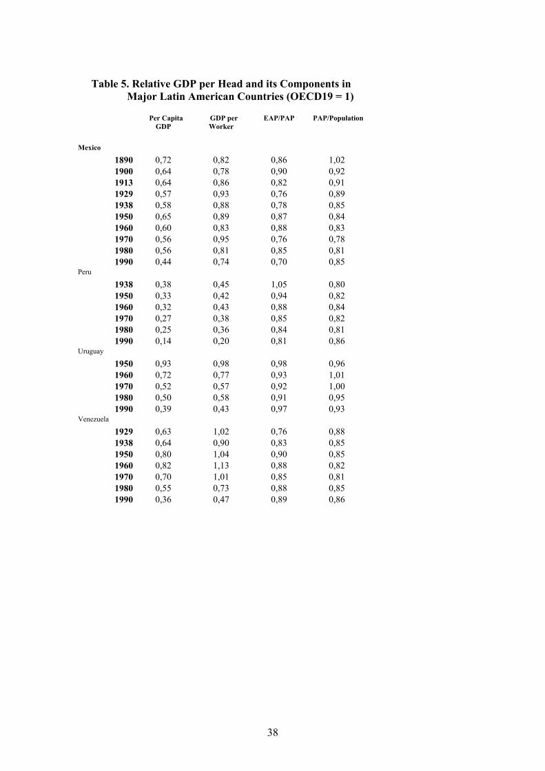
Table 5. Relative GDP per Head and its Components in

Major Latin American Countries (OECD19 = 1)

Per Capita GDP

GDP per Worker

EAP/PAP PAP/Population

Mexico

1890 0,72 0,82 0,86 1,02 1900 0,64 0,78 0,90 0,92 1913 0,64 0,86 0,82 0,91 1929 0,57 0,93 0,76 0,89 1938 0,58 0,88 0,78 0,85 1950 0,65 0,89 0,87 0,84 1960 0,60 0,83 0,88 0,83 1970 0,56 0,95 0,76 0,78 1980 0,56 0,81 0,85 0,81 1990 0,44 0,74 0,70 0,85

Peru

1938 0,38 0,45 1,05 0,80 1950 0,33 0,42 0,94 0,82 1960 0,32 0,43 0,88 0,84 1970 0,27 0,38 0,85 0,82 1980 0,25 0,36 0,84 0,81 1990 0,14 0,20 0,81 0,86

Uruguay

1950 0,93 0,98 0,98 0,96 1960 0,72 0,77 0,93 1,01 1970 0,52 0,57 0,92 1,00 1980 0,50 0,58 0,91 0,95 1990 0,39 0,43 0,97 0,93

Venezuela

1929 0,63 1,02 0,76 0,88 1938 0,64 0,90 0,83 0,85 1950 0,80 1,04 0,90 0,85 1960 0,82 1,13 0,88 0,82 1970 0,70 1,01 0,85 0,81 1980 0,55 0,73 0,88 0,85 1990 0,36 0,47 0,89 0,86

38

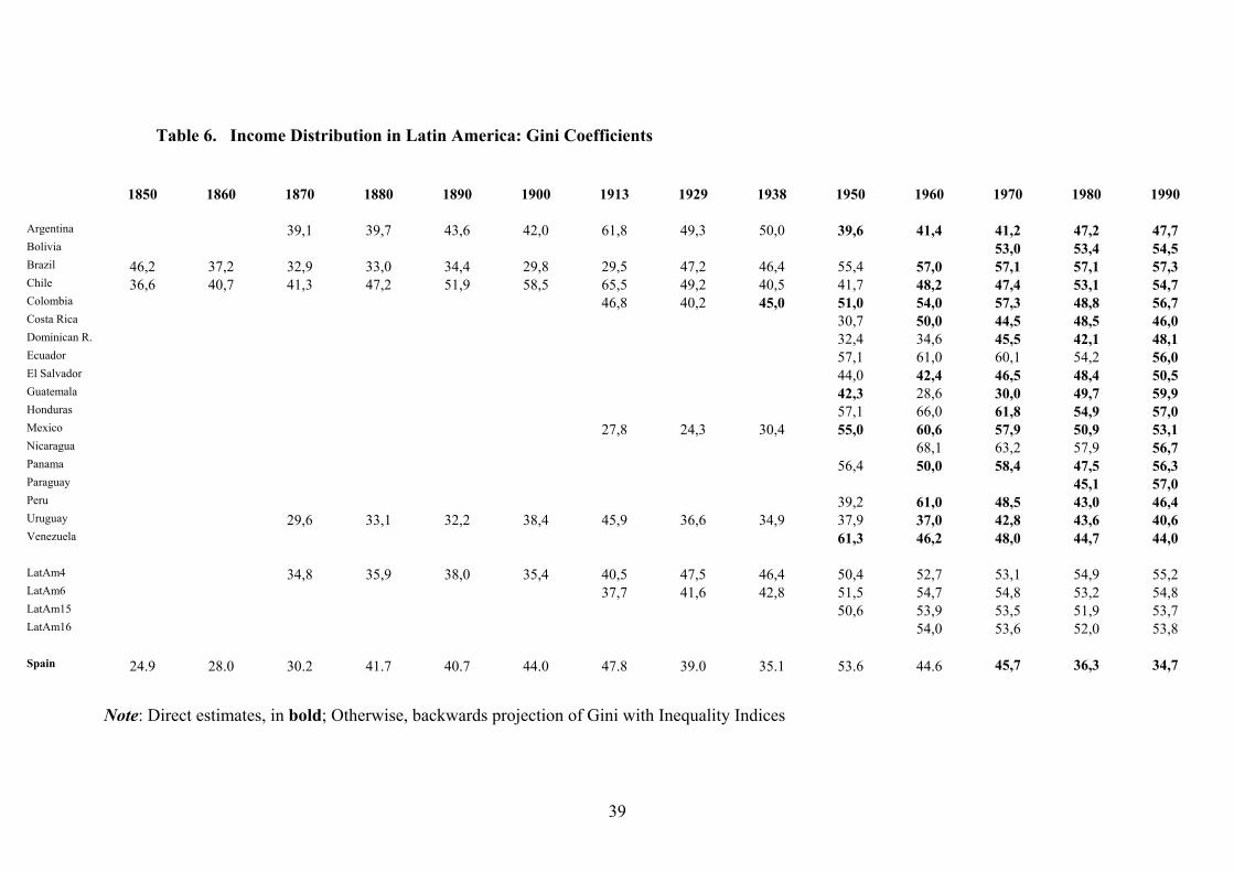
Table 6. Income Distribution in Latin America: Gini Coefficients

1850

1860 1870 1880 1890 1900 1913 1929 1938 1950 1960 1970 1980 1990

Argentina 39,1 39,7 43,6 42,0 61,8 49,3 50,0 39,6 41,4 41,2 47,2 47,7Bolivia 53,0 53,4 54,5Brazil 46,2 37,2 32,9 33,0 34,4 29,8 29,5 47,2 46,4 55,4 57,0 57,1 57,1 57,3Chile 36,6 40,7 41,3 47,2 51,9 58,5 65,5 49,2 40,5 41,7 48,2 47,4 53,1 54,7Colombia 46,8 40,2 45,0 51,0 54,0 57,3 48,8 56,7Costa Rica 30,7 50,0 44,5 48,5 46,0Dominican R. 32,4 34,6 45,5 42,1 48,1Ecuador 57,1 61,0 60,1 54,2 56,0 El Salvador 44,0 42,4 46,5 48,4 50,5Guatemala 42,3 28,6 30,0 49,7 59,9Honduras 57,1 66,0 61,8 54,9 57,0Mexico 27,8 24,3 30,4 55,0 60,6 57,9 50,9 53,1Nicaragua 68,1 63,2 57,9 56,7 Panama 56,4 50,0 58,4 47,5 56,3Paraguay 45,1 57,0Peru 39,2 61,0 48,5 43,0 46,4Uruguay 29,6 33,1 32,2 38,4 45,9 36,6 34,9 37,9 37,0 42,8 43,6 40,6Venezuela 61,3 46,2 48,0 44,7 44,0

LatAm4 34,8 35,9 38,0 35,4 40,5 47,5 46,4 50,4 52,7 53,1 54,9 55,2 LatAm6 37,7 41,6 42,8 51,5 54,7 54,8 53,2 54,8LatAm15 50,6 53,9 53,5 51,9 53,7LatAm16 54,0 53,6 52,0 53,8

Spain 24.9 28.0 30.2 41.7 40.7 44.0 47.8 39.0 35.1 53.6 44.6 45,7 36,3 34,7

Note: Direct estimates, in bold; Otherwise, backwards projection of Gini with Inequality Indices

39

Table 7. Share of Economically Active Population in Agriculture

1900

1913 1929 1938 1950 1960 1970 1980 1990Argentina 0,39 0,35 0,36 0,35 0,25 0,21 0,16 0,13 0,12Bolivia 0,56 0,55 0,55 0,53 0,47Brazil 0,71 0,69 0,62 0,55 0,47 0,37 0,23Chile 0,37 0,37 0,37 0,36 0,33 0,30 0,24 0,21 0,19Colombia 0,73 0,59 0,52 0,45 0,40 0,27Costa Rica 0,57 0,51 0,43 0,35 0,26Cuba 0,41 0,36 0,30 0,24 0,18Dominican Republic 0,73 0,64 0,48 0,32 0,25Ecuador 0,65 0,59 0,52 0,40 0,33El Salvador 0,65 0,62 0,57 0,44 0,36Guatemala 0,69 0,66 0,61 0,54 0,52Haiti 0,86 0,80 0,74 0,71 0,68Honduras 0,75 0,72 0,67 0,57 0,41Mexico 0,62 0,68 0,70 0,66 0,66 0,54 0,50 0,36 0,35Nicaragua 0,70 0,63 0,51 0,40 0,29Panama 0,56 0,51 0,42 0,29 0,26Paraguay 0,54 0,54 0,50 0,45 0,39Peru 0,58 0,52 0,48 0,40 0,36Uruguay 0,24 0,21 0,19 0,17 0,14Venezuela 0,59 0,54 0,43 0,33 0,26 0,15 0,12

Sources: OxLAD (2004).

40

Table 8. Relative Labor Productivity in Agriculture

1900

1913 1929 1938 1950 1960 1970 1980 1990Argentina 0,74 0,70 0,64 0,62 0,68 0,77 0,82 0,85 1,20Bolivia 0,46 0,44 0,31 0,28 0,32Brazil 0,32 0,33 0,27 0,24 0,21 0,20 0,34Chile 0,44 0,42 0,32 0,40 0,34 0,32 0,33 0,35 0,43Colombia 0,64 0,64 0,63 0,63 0,62 0,91Costa Rica 0,67 0,58 0,59 0,58 0,84Cuba 0,51 0,52 0,64 0,52 0,51Dominican Republic 0,47 0,53 0,54 0,57 0,64Ecuador 0,64 0,66 0,58 0,53 0,78El Salvador 0,63 0,58 0,54 0,77 0,86Guatemala 0,53 0,51 0,49 0,50 0,51Haiti 0,61 0,62 0,68 0,56 0,58Honduras 0,60 0,45 0,51 0,53 0,75Mexico 0,45 0,37 0,28 0,30 0,28 0,30 0,23 0,24 0,22Nicaragua 0,52 0,47 0,53 0,75 1,09Panama 0,58 0,51 0,38 0,48 0,59Paraguay 0,75 0,73 0,69 0,64 0,80Peru 0,40 0,47 0,39 0,36 0,57Uruguay 0,56 0,52 0,68 0,64 0,78Venezuela 0,40 0,22 0,24 0,29 0,49 0,68

Sources: computed from OxLAD (2004).

41

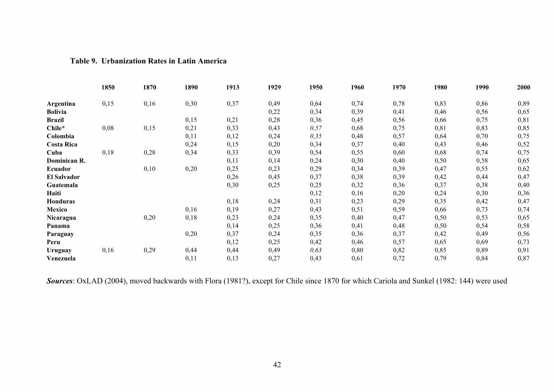
Table 9. Urbanization Rates in Latin America

1850

1870 1890 1913 1929 1950 1960 1970 1980 1990 2000

Argentina 0,15 0,16 0,30 0,37 0,49 0,64 0,74 0,78 0,83 0,86 0,89 Bolivia 0,22 0,34 0,39 0,41 0,46 0,56 0,65Brazil 0,15 0,21 0,28 0,36 0,45 0,56 0,66 0,75 0,81Chile* 0,08 0,15 0,21 0,33 0,43 0,57 0,68 0,75 0,81 0,83 0,85Colombia 0,11 0,12 0,24 0,35 0,48 0,57 0,64 0,70 0,75Costa Rica 0,24 0,15 0,20 0,34 0,37 0,40 0,43 0,46 0,52Cuba 0,18 0,28 0,34 0,33 0,39 0,54 0,55 0,60 0,68 0,74 0,75Dominican R. 0,11 0,14 0,24 0,30 0,40 0,50 0,58 0,65Ecuador 0,10 0,20 0,25 0,23 0,29 0,34 0,39 0,47 0,55 0,62El Salvador 0,26 0,45 0,37 0,38 0,39 0,42 0,44 0,47Guatemala 0,30 0,25 0,25 0,32 0,36 0,37 0,38 0,40Haiti 0,12 0,16 0,20 0,24 0,30 0,36Honduras 0,18 0,24 0,31 0,23 0,29 0,35 0,42 0,47Mexico 0,16 0,19 0,27 0,43 0,51 0,59 0,66 0,73 0,74Nicaragua 0,20 0,18 0,23 0,24 0,35 0,40 0,47 0,50 0,53 0,65Panama 0,14 0,25 0,36 0,41 0,48 0,50 0,54 0,58Paraguay 0,20 0,37 0,24 0,35 0,36 0,37 0,42 0,49 0,56Peru 0,12 0,25 0,42 0,46 0,57 0,65 0,69 0,73Uruguay 0,16 0,29 0,44 0,44 0,49 0,63 0,80 0,82 0,85 0,89 0,91Venezuela 0,11 0,13 0,27 0,43 0,61 0,72 0,79 0,84 0,87

Sources: OxLAD (2004), moved backwards with Flora (1981?), except for Chile since 1870 for which Cariola and Sunkel (1982: 144) were used

42

Table 10. Relative Rural Income per Head (GDP per Capita = 1) 1900

1913 1929 1950 1960 1970 1980 1990 2000

Argentina 0,41 0,39 0,45 0,48 0,60 0,61 0,65 1,08 1,08Bolivia 0,39 0,40 0,29 0,27 0,34 0,39Brazil 0,29 0,32 0,26 0,24 0,23 0,21 0,31 0,47Chile 0,21 0,23 0,21 0,26 0,30 0,32 0,39 0,48 0,40Colombia 0,60 0,60 0,65 0,58 0,63 0,67 0,70 0,79 0,84Costa Rica 0,25 0,58 0,47 0,42 0,36 0,40 0,25Cuba 0,45 0,41 0,48 0,38 0,35 0,31Dominican R. 0,45 0,48 0,43 0,37 0,38 0,39Ecuador 0,59 0,60 0,49 0,40 0,58 0,66El Salvador 0,79 0,65 0,58 0,51 0,57 0,56 0,42Guatemala 0,48 0,49 0,49 0,47 0,43 0,44 0,41Haiti 0,60 0,58 0,63 0,52 0,56 0,57Honduras 0,74 0,65 0,42 0,49 0,47 0,53 0,52Mexico 0,33 0,25 0,27 0,32 0,33 0,29 0,25 0,28 0,26Nicaragua 0,87 0,56 0,49 0,51 0,60 0,67 1,05Panama 0,51 0,44 0,30 0,28 0,33 0,29Paraguay 0,62 0,61 0,54 0,49 0,61 0,70Peru 0,39 0,45 0,44 0,41 0,66 0,85Uruguay 0,36 0,55 0,71 0,71 0,99 1,15Venezuela 0,16 0,20 0,26 0,35 0,51 0,59

Sources: See the text.

43

Table 11. Average Income/Poverty Line Ratio in Latin America (Poverty Line: 1985 G-K $ 4 a day) 1850

1860 1870 1880 1890 1900 1913 1929 1938 1950 1960 1970 1980 1990Argentina 0,7 0,8 1,3 1,2 1,7 1,9 1,8 2,2 2,5 3,6 4,5 3,5Bolivia 0,8 0,6 0,9 1,1 1,0Brazil 0,4 0,4 0,4 0,4 0,4 0,4 0,5 0,7 0,7 0,9 1,3 1,7 3,0 3,0Chile 0,4 0,5 0,6 0,9 0,9 1,1 1,4 1,7 1,5 1,8 2,1 2,5 2,8 3,1Colombia 0,4 0,5 0,9 1,0 1,2 1,4 1,8 2,4 2,7Costa Rica 0,9 0,9 1,1 1,1 1,4 1,9 2,6 2,6Dominican R. 0,7 0,9 1,1 1,6 1,4Ecuador 0,4 0,5 0,7 0,7 1,1 1,3 1,5 2,3 2,2El Salvador 0,5 0,6 0,5 0,8 1,0 1,2 1,3 1,1Guatemala 0,7 0,8 1,1 1,0 1,1 1,4 1,8 1,6Haiti 0,4 0,5 0,4 0,6 0,4Honduras 0,6 0,8 0,6 0,7 0,8 0,9 1,0 1,0Mexico 0,6 0,5 0,6 0,6 1,0 1,0 1,2 1,4 1,4 2,1 2,7 3,8 4,9 4,8Nicaragua 0,8 1,4 0,8 1,3 1,6 2,5 1,7 1,0Panama 1,1 1,3 2,0 2,5 2,3Paraguay 0,8 0,8 0,8 1,0 1,6 1,7Peru 0,4 0,5 0,9 0,9 1,1 1,4 1,8 2,1 1,5Uruguay 1,2 1,2 1,3 1,5 2,2 2,5 2,6 3,1 3,3 3,5 4,3 4,3Venezuela 0,3 0,3 0,2 0,3 0,4 0,4 0,5 1,5 1,6 2,6 3,7 4,7 4,7 3,9

LA4 0,5 0,4 0,5 0,5 0,7 0,7 0,8 1,0 1,0 1,4 1,9 2,6 3,7 3,7LA6 0,5 0,6 0,8 0,7 1,0 1,2 1,2 1,6 2,0 2,7 3,8 3,7LA10 0,7 0,9 1,1 1,2 1,5 1,9 2,5 3,5 3,4LA14 0,9 1,1 1,1 1,5 1,8 2,5 3,4 3,3LA19 1,4 1,8 2,4 3,3 3,1

Spain 0,6 0,7 0,7 1,0 1,0 1,0 1,2 1,6 1,0 1,3 1,8 3,6 5,3 7,0

OECD15 0,8 1,0 1,1 1,4 1,5 1,8 2,2 2,7 2,7 3,9 5,1 7,2 9,1 11,2OECD19 1,0 1,2 1,4 1,6 1,9 2,4 2,4 3,3 4,5 6,8 8,7 10,9OECD21 2,4 2,4 3,3 4,5 6,7 8,6 10,9

44

Table 12. Poverty Headcount in Latin America (1985 G-K $ 4 a day): A Calibration (%)

1850

65 71

44 54

1860 1870 1880 1890 1900 1913 1929 1938 1950 1960 1970 1980 1990Argentina 64 60 53 56 58 41 45 24 22 10 11 17Bolivia Brazil 93 96 96 96 95 98 93 82 79 75 64 53 33 34Chile 94 89 84 74 71 70 65 47 42 36 36 28 31 29Colombia 90 70 65 61 57 52 32 37Costa Rica 54 55 35 28 25Dominican R. 83 71 64 43 53Ecuador 87 84 79 66 43El Salvador 74 66 58 58 64Guatemala 63 52 37 44 59Honduras 80 80 76 70 71Mexico 43 31 36 43 41 27 13 15Nicaragua 64 47 53 70Panama 69 58 48 28 42Paraguay Peru 60 62 43 29 48Uruguay 45 48 42 43 32 15 12 11 8 12 8 6Venezuela 43 14 11 8 11

LatAm4 89 85 84 85 81 67 66 59 52 43 29 30LatAm6 71 59 60 55 50 40 25 27LatAm15 57 51 41 27 30LatAm16 51 41 27 30

Spain 88 81 81 67 67 64 60 39 62 62 39 14 2 0

Sources: See text.

45

46

Graph 1. GDP per head in Latin America (1980 G-K $)

0

1000

2000

3000

4000

5000

6000

1850 1860 1870 1880 1890 1900 1913 1925 1929 1938 1950 1960 1970 1975 1980 1990 2000

LA4 LA6 LA10 LA14 LA19

47

Graph 2. Trends in GDP per Head: 8 Major Latin American Countries (1980 G-K $)

0

1000

2000

3000

4000

5000

6000

7000

1850 1860 1870 1880 1890 1900 1913 1925 1929 1938 1950 1960 1970 1975 1980 1990 2000

Argentina Brazil Chile Colombia Mexico Peru Uruguay Venezuela

48

Graph 3. Relative GDP per Head in Latin America (OECD = 1)

0,00

0,10

0,20

0,30

0,40

0,50

0,60

1850 1860 1870 1880 1890 1900 1913 1925 1929 1938 1950 1960 1970 1975 1980 1990 2000

RLA4 RLA6 RLA10 RLA14 RLA19

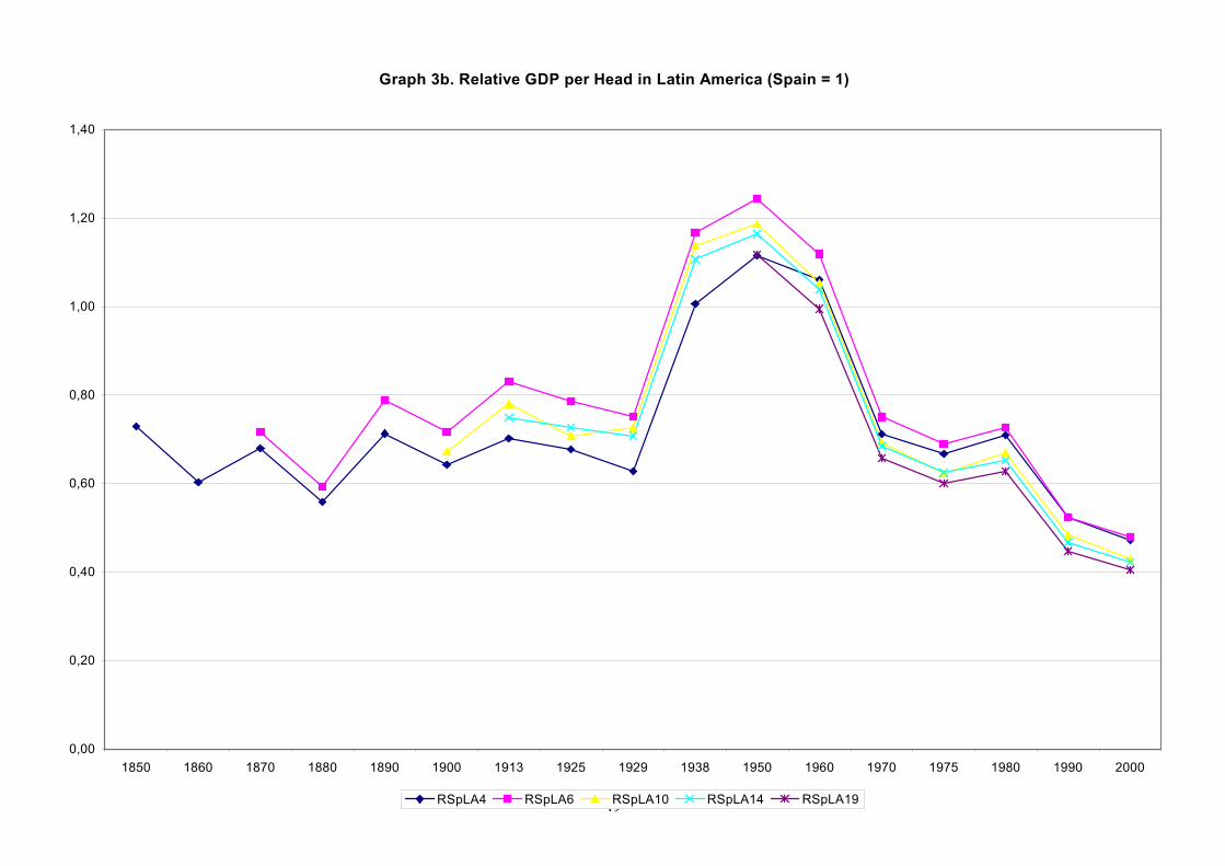
49

Graph 3b. Relative GDP per Head in Latin America (Spain = 1)

0,00

0,20

0,40

0,60

0,80

1,00

1,20

1,40

1850 1860 1870 1880 1890 1900 1913 1925 1929 1938 1950 1960 1970 1975 1980 1990 2000

RSpLA4 RSpLA6 RSpLA10 RSpLA14 RSpLA19

Graph 4. Relative GDP per Head in 8 Major Latin American Countries (OECD15 = 1)

0,00

0,20

0,40

0,60

0,80

1,00

1,20

1850 1860 1870 1880 1890 1900 1913 1925 1929 1938 1950 1960 1970 1975 1980 1990 2000

Argentina Brazil Chile Colombia Mexico Peru Uruguay Venezuela

50

Graph 4b. Relative GDP per Head in 8 Major Latin American Countries (Spain = 1)

0,00

0,50

1,00

1,50

2,00

2,50

3,00

1850 1860 1870 1880 1890 1900 1913 1925 1929 1938 1950 1960 1970 1975 1980 1990 2000

Argentina Brazil Chile Colombia Mexico Peru Uruguay Venezuela

51

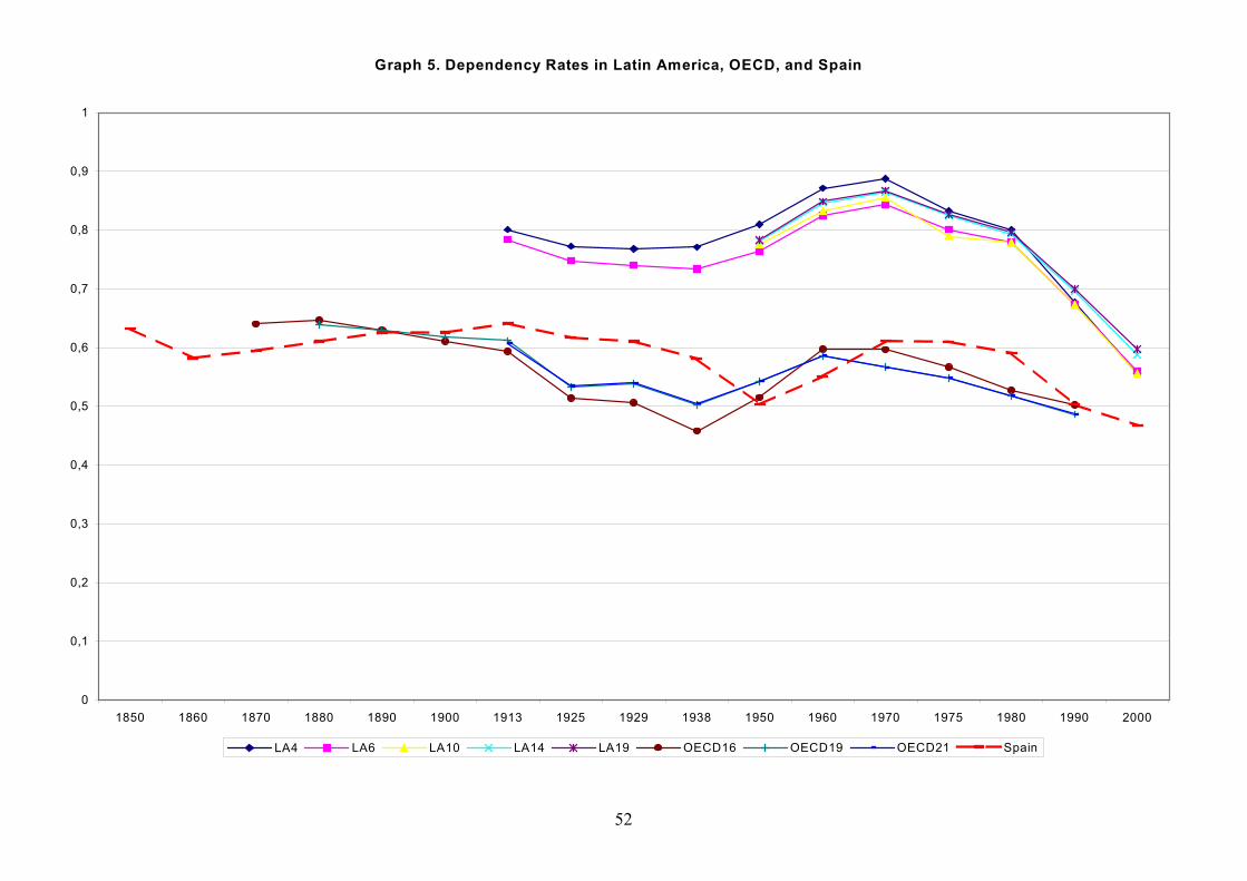
Graph 5. Dependency Rates in Latin America, OECD, and Spain

0

0,1

0,2

0,3

0,4

0,5

0,6

0,7

0,8

0,9

1

1850 1860 1870 1880 1890 1900 1913 1925 1929 1938 1950 1960 1970 1975 1980 1990 2000

LA4 LA6 LA10 LA14 LA19 OECD16 OECD19 OECD21 Spain

52

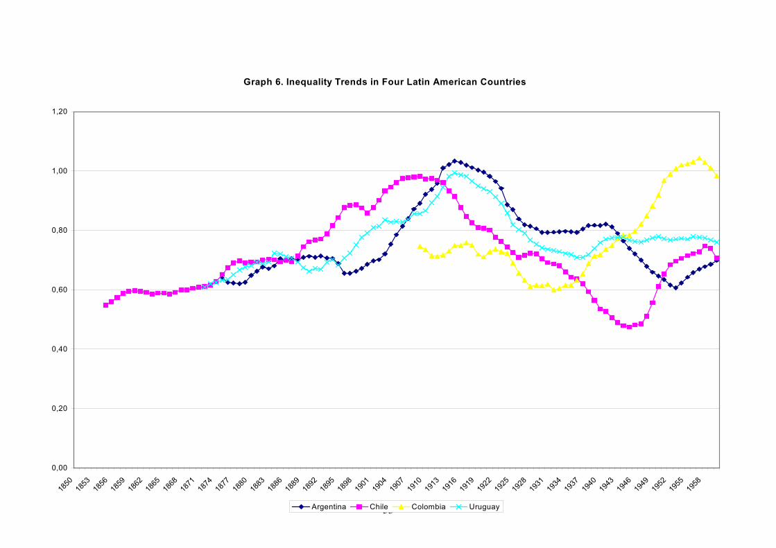
53

Graph 6. Inequality Trends in Four Latin American Countries

0,00

0,20

0,40

0,60

0,80

1,00

1,20

1850

1853

1856

1859

1862

1865

1868

1871

1874

1877

1880

1883

1886

1889

1892

1895

1898

1901

1904

1907

1910

1913

1916

1919

1922

1925

1928

1931

1934

1937

1940

1943

1946

1949

1952

1955

1958

Argentina Chile Colombia Uruguay

Graph 6b. Inequality Index in Brazil, Cuba, and Mexico

0,00

0,50

1,00

1,50

2,00

2,50

3,00

3,50

4,00

1850

1853

1856

1859

1862

1865

1868

1871

1874

1877

1880

1883

1886

1889

1892

1895

1898

1901

1904

1907

1910

1913

1916

1919

1922

1925

1928

1931

1934

1937

1940

1943

1946

1949

1952

1955

1958

Brazil Mexico Cuba

54

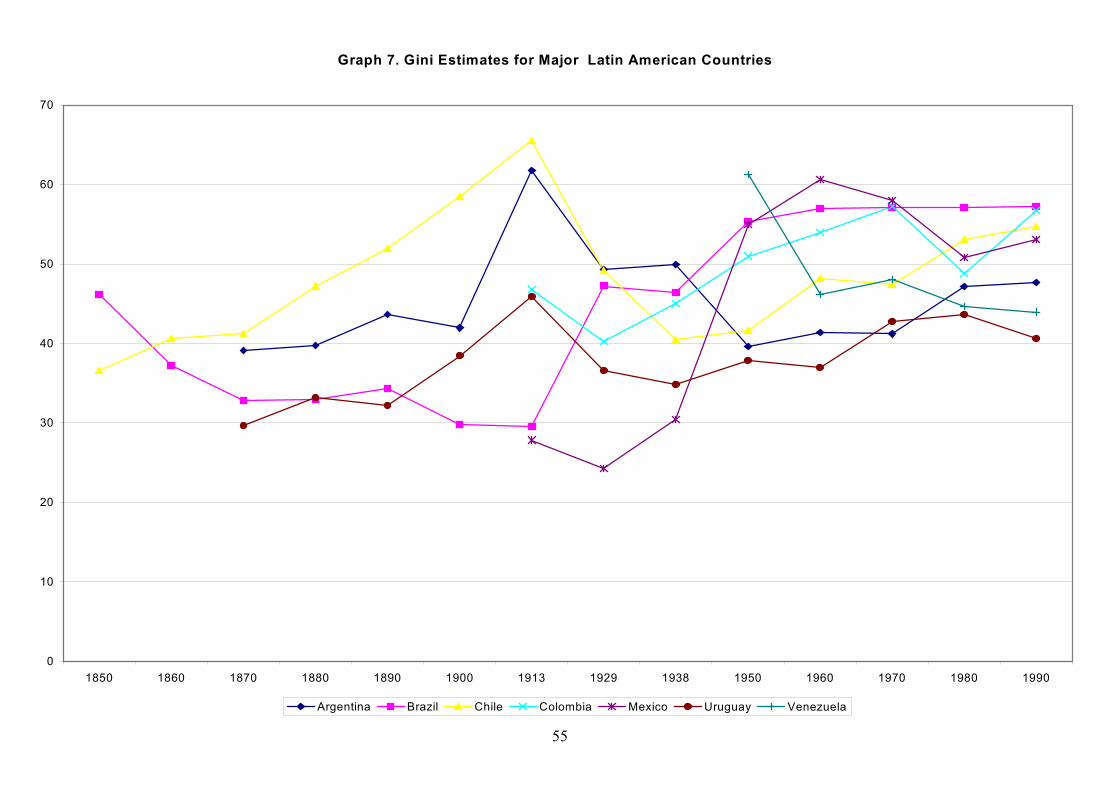
Graph 7. Gini Estimates for Major Latin American Countries

0

10

20

30

40

50

60

70

1850 1860 1870 1880 1890 1900 1913 1929 1938 1950 1960 1970 1980 1990

Argentina Brazil Chile Colombia Mexico Uruguay Venezuela

55

56

Graph 7b. Gini Estimates for Latin America and Spain

0

10

20

30

40

50

60

1850 1860 1870 1880 1890 1900 1913 1929 1938 1950 1960 1970 1980 1990

LatAm4 LatAm6 LatAm15 LatAm16 Spain

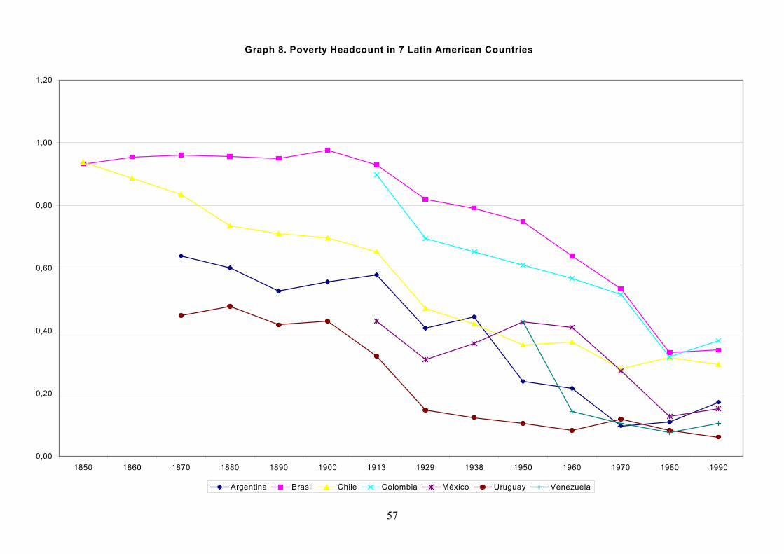
Graph 8. Poverty Headcount in 7 Latin American Countries

0,00

0,20

0,40

0,60

0,80

1,00

1,20

1850 1860 1870 1880 1890 1900 1913 1929 1938 1950 1960 1970 1980 1990

Argentina Brasil Chile Colombia México Uruguay Venezuela

57

58

Graph 8b. Poverty Headcount in Latin America and Spain (Poverty Line: 1980 G-K $ 4 a day)

0

10

20

30

40

50

60

70

80

90

100

1850 1860 1870 1880 1890 1900 1913 1929 1938 1950 1960 1970 1980 1990

LatAm4 LatAm6 LatAm15 LatAm16 Spain