Growth, Income Distribution and Democracy:What the Data Say

by

Roberto Perotti, Columbia University

September 1995

1994-95 Discussion Paper Series No. 757

Growth, income distribution, and democracywhat the data say.

Roberto Perotti

Columbia University

First version: March 1995

This version: September 1995

I thank Alberto Alesina, Oded Galor, Andy Newman, Torsten Persson, two anonymous

referees, and participants at the 1995 NBER Growth Conference in Barcelona and 1995

NBER Summer Institute for comments.

1 Introduction.

This paper investigates the relationship between income distribution, democratic institu-

tions, and growth. It does so by addressing three main issues. First, the properties and

reliability of the income distribution data; second, the robustness of the reduced form re-

lationships between income distribution and growth estimated so far; third, the specific

channels through which income distribution affects growth.

The theoretical literature on income distribution and growth has expanded enormously

in recent years * on the empirical side, however, progress has been much slower. Probably

the most important reason has been the perceived limitations of existing cross-section

data on income distribution, both in terms of availability of observations and in terms of

their quality. A discussion of the income distribution datasets currently used and of their

comparative properties is therefore fundamental for an evaluation of the existing empirical

evidence.

Practically all this evidence consists of reduced form estimates that add income distribu-

tion variables to the set of independent variables of otherwise standard growth regressions.

In the vast majority of these estimates, equality has a positive impact on growth. The

second important issue studied in this paper is precisely the robustness of this positive

reduced form relationship between equality and growth.

Other properties of the reduced form have been more controversial. For instance, several

theories postulate a different relationship between equality and growth in democracies

and non-democracies. Different empirical studies have reached opposite conclusions on

this point. To what extent are these contrasting results due to differences in the income

distribution data used, and to what extent are they due to differences in the specification

and in the samples? A conclusion of the paper is that specification issues, rather than data,

are crucial in this respect.

The theoretical literature provides an array of very different explanations for the pos-

itive correlation between equality and growth. By its nature, a reduced form estimate

and Perotti (1994) and Perotti (1994a) provide two short surveys of some recent developmentsin this field.

cannot shed light on the underlying mechanisms. Hence the importance of the third issue

- evaluating the specific channel(s) of operation of income distribution by estimating the

structural models behind the reduced form. The paper explores the four channels that

have emerged in the literature: endogenous fiscal policy, socio-political instability, borrow-

ing constraints, and endogenous fertility. The main conclusion in this regard is that there

is strong empirical support for two types of explanations, linking income distribution to

socio-political instability and to the education/fertility decision. A third channel, based

on capital market imperfection, also seems to receive some support by the data, although

it is probably the hardest to test with the existing data. By contrast, there appears to be

less empirical support for explanations based on the effects of income distribution on fiscal

policy and on capital market imperfections.

The plan of this paper is as follows. The next section briefly surveys the main re-

cent theories on income distribution and growth. Section 3 presents and discusses the

income distribution data used throughout this paper. Section 4 studies extensively the

reduced form relationship between income distribution and growth. Sections 5, 6, and 7

study the approaches based on fiscal policy, socio-political instability, and imperfect capital

markets/endogenous fertility, respectively. Section 8 concludes.

2 A very brief survey of the main approaches.

At the risk of some oversimplification, the recent literature on income distribution and

growth can be divided into three main approaches: the "fiscal policy", "socio-political in-

stability", and "imperfect capital market" approaches. A fourth approach, which deals

with the relationship between income distribution on one side and human capital invest-

ment and fertility decisions on the other, has not been fully formalized, to the best of my

knowledge. However, for the purposes of this paper one can speculate what this relationship

might be by applying simple compositional arguments to a well established, representative

agent literature. For lack of a better name, this approach can be called the "endogenous

fertility" approach.

In the fiscal policy approach of Alesina and Rodrik (1994), Bertola (1993), Perotti

(1993), Persson and Tabellini (1994), and many others, income distribution affects growth

via its effects on government expenditure and taxation. For the sake of brevity, consider

a highly stylized framework where fiscal policy is decided by majority voting, taxation

is proportional to income, and tax revenues are redistributed lump-sum to all individuals.

Thus, the tax rate and the level of the benefit are positively related through the government

budget constraint.

This type of fiscal policy is redistributive because the taxes an individual pays are

proportional to his income; the benefits of expenditure, however, accrue equally to all

individuals. Consequently, the level of taxation and expenditure preferred by an individual

are inversely related to his income. Since this is also true for the median voter - the decisive

voter under some well-known conditions -, in equilibrium the median income on one side and

the level of expenditure and taxation on the other are negatively related. This relationship

between the income of the median voter and the level of expenditure and taxation, via the

political process, constitutes the first logical component of the fiscal policy approach, or its

"political mechanism".

In turn, redistributive government expenditure and taxation are negatively related to

growth, primarily because of their disincentive effects on private savings and investment.

The second logical component of the fiscal policy approach is this negative link between

government expenditure and growth, which can be termed its "economic mechanism".

In summary, in a more equal society there is less demand for redistribution (the political

mechanism), and therefore lower taxation and more investment and growth (the economic

mechanism). Thus, the fiscal policy approach posits a positive reduced form relationship

between equality and growth.

The fiscal policy approach can then be summarized in three simple results ("FP" stands

for "fiscal policy"):

Result FP1 (the economic mechanism): Growth increases as distortionary taxation de-

creases;

Result FP2 (the political mechanism): Redistributive government expenditure and there-

fore distortionary taxation decrease as equality increases;

Result FP3 (the reduced form): Growth increases as equality increases.

Most of the existing literature can be interpreted as estimating FP3;2 this paper goes

beyond this by estimating FP1 and FP2, and similarly for the other approaches.

The fiscal policy approach also implies a fundamental distinction between democracies,

where in the long run fiscal policy reflects the preferences of the majority and therefore the

distribution of income, and non-democracies, where the link between income distribution

and fiscal policy is, at most, indirect. In other words, the effect of the fiscal policy variable

in the political mechanism and in the reduced form should be stronger in democracies.

This is a testable implication of the model, which will be exploited in the next sections.

According to the socio-political instability approach of Alesina and Perotti (1995),

Gupta (1990), Hibbs (1973), Venieris and Gupta (1983) and (1986), and others, a highly

unequal, polarized distribution of resources creates strong incentives for organized individ-

uals to pursue their interests outside the normal market activities or the usual channels

of political representation. Thus, in more unequal societies individuals are more prone to

engage in rent-seeking activities, or other manifestations of socio-political instability, like

violent protests, assassinations, coups, etc.

In turn, socio-political instability discourages investment for at least two classes of

reasons. First, it creates uncertainty regarding the political and legal environment. Second,

it disrupts market activities and labor relations, with a direct adverse effect on productivity.

Theoretical models that formalize these or related ideas include Benhabib and Rustichini

(1991), Fay (1993), Tornell and Lane (1994) and Svensson (1994).

Like the fiscal policy approach, the socio-political instability approach can be summa-

rized in three results ("SPI" stands for "socio-political instability"):

Result SP1: Investment and growth increase as socio-political instability decreases;

Result SP2: Socio-political instability decreases as equality increases;

Result SP3 (the reduced form): Growth increases as equality increases.

2The only exception I am aware of is Persson and Tabellini (1994), who however have only 11 and 10degrees of freedom in their regressions for FP1 and FP2, respectively. The coefficients they estimate arenever significant.

Thus, the socio-political instability approach too posits a positive reduced form rela-

tionship between equality and growth, although the underlying mechanisms are markedly

different from the fiscal policy approach.

A sizable strand of recent research has emphasized the link between capital market

imperfections, the distribution of income and wealth and a society's aggregate investment

in human and other forms of capital. A very partial list of contributions includes Aghion

and Bolton (1993), Galor and Zeira (1993), Banerjee and Newman (1991) and (1993). The

basic idea that emerges from these models is simple: when individuals cannot borrow freely

against future income, the initial distribution of resources can have a large impact on the

economy's pattern of investment and therefore of growth. A fairly general, although not

universal, conclusion of these models is that, if wealth is distributed more equally, more

individuals are able to invest in human capital, and consequently growth is higher.3

This relationship would persist in the long-run under two main sets of circumstances. If

there are fixed costs of investment in education, a dynasty that starts out poor and cannot

invest in education, will keep doing so generation after generation. However, one could

argue that the direct costs of education are negligible for primary and, in most countries,

even secondary education. The largest component of the cost of education, particularly

secondary education, is foregone income. In this case, if the marginal utility of consumption

at very low levels of consumption is very high, poor individuals who cannot borrow will not

invest in education. Since their children will start out in the same position, that dinasty

will be caught in a poverty trap, with no investment in human capital (see De Gregorio

(1994) for a representative agent model based on this mechanism).

The distribution of income and wealth also affect how pervasive borrowing constraints

are in an economy. If utility is bounded from below, poor individuals might be unable to

borrow because of the incentive problems borrowing creates (see Banerjee and Newman

(1994)). In this case, the distribution of income and wealth will also determine how many

3This conclusion is subject to at least one important qualification: in very poor societies, it mightbe the case that only the rich can possibly invest in education. Therefore, investment in human capitalwould be maximized if wealth were concentrated in the hands of the rich. In this case, growth would bepositively related to inequality: see Aghion and Bolton (1993) and Perotti (1993) for models based on thismechanism.

individuals are close to the lower bound and therefore are unable to borrow.

Although this approach deals primarily with the distribution of wealth, its empirical

implications can be stated in terms of the distribution of income because of the large

correlation between indicators of equality derived from the two distributions. Like the other

two, this approach can then be summarized in three results ("ICM" stands for "imperfect

capital markets"):

Result ICM1: Growth increases as investment in human capital increases;

Result ICM2: For any given degree of imperfection in the capital market, investment in

human capital increases as equality increases;

Result ICM3 (the reduced form): Growth increases as equality increases.

In an optimizing model, investment in education and fertility would be strictly con-

nected because they can be interpreted as two alternative uses of the parents' human

capital: the former, in the quality of the immediate descendants, the latter, in their quan-

tity. In spite of this close theoretical link, demographic factors, and in particular fertility,

have been largely ignored in the literature on income distribution and growth. Galor and

Zang (1993) is the only contribution that deals with the interaction of income distribution,

imperfect capital markets, schooling and fertility simultaneously. In their model, given the

distribution of income, a higher fertility means that less resources are available within each

family to finance the education of each child; with fixed costs of education and borrowing

constraints, fewer children will be able to attend school. Similarly, given the fertility rate,

a more skewed distribution of income is associated with lower enrollment ratios because

of the inability to borrow against future income. Fertility, however, is not endogenized in

their model.

The joint decision about fertility and schooling has been studied extensively in the

context of representative agent models of growth (see, for instance, Becker and Barro (1988)

and Becker, Murphy and Tamura (1991)). By interpreting the representative agent of these

models as a dynasty, and by varying the initial human capital of a dynasty, using a simple

compositional argument one can speculate on the predictions of these models regarding

the relationship between the distribution of human capital on one side and human capital

6

investment and fertility on the other.

Fertility and schooling decisions are the result of the interplay of the direct cost of

raising children and the opportunity cost of the parents' human capital. An increase in

the human capital of the parents has two effects on fertility. The income effect implies a

higher demand for children; on the other hand, the opportunity cost of raising children

increases, and therefore the substitution effect implies a lower demand for children. At

low levels of human capital, the direct cost is the main component of the total costs of

raising children, inclusive of the opportunity costs. Therefore, an increase in the parents'

human capital has little effect on the total costs of raising children and the income effect

prevails. At high levels of human capital, the substitution effect of an increase in human

capital prevails because the direct cost of raising children is a relatively small part of the

total costs. Thus, at sufficiently high levels of human capital, an increase in human capital

leads to less fertility and higher investment in human capital.

Now imagine a redistribution of human capital from individuals that have a high en-

dowment to individuals with a low endowment of human capital, and suppose that the

substitution effect of an increase in human capital prevails. The rate of return to invest-

ment in education for poor individuals would increase, and their demand for children would

fall. This would likely increase aggregate enrollment ratios and decrease fertility if, at low

levels of human capital, the demand for children is sufficiently elastic to human capital

and the demand for human capital investment is sufficiently elastic to the rate of return.

Thus, one could speculate that a reasonable extension of these models to a non-degenerate

distribution of income would predict a negative relationship between equality and fertility,

and a positive relationship between equality and investment in human capital. The higher

investment in human capital would also lead to higher growth.

One can try to summarize these conclusions in the following results: ("EF" stands for

" endogenous fertility"):

Result EF1: Growth increases as investment in human capital increases and fertility de-

creases;

Result EF2: Fertility decreases and investment in human capital increases as equality in-

creases;

Result EF3 (the reduced form): Growth increases as equality increases.

Notice that results FP3, SPI3, ICM3, and EF3 are identical: in other words, all four

approaches predict the same positive relationship between equality and growth. The un-

derlying mechanisms, however, are markedly different, which motivates the empirical in-

vestigation of this paper.

3 The income distribution data.

In testing the theories surveyed above, two preliminary problems arise. First, as it was

mentioned above, in several cases the relevant distribution is that of wealth rather than

income. Data on the distribution of wealth do not exist for a sufficient number of countries,

and the distribution of income must be used as a proxy. Empirically, however, this is

unlikely to be a serious problem because the shapes of the two distributions generally vary

together in cross-sections, although the former tends to be more skewed than the latter.

The second problem is that in many of the theories surveyed above, the effect of income

distribution on growth might depend on the whole shape of the distribution of income. In

addition, it is well known that widely used compact measures of the distribution of income

might not always provide an unambiguous ranking according to a specific criterion: for

instance, this would be the case if the Gini coefficient were used and the underlying Lorenz

curves intersect. Thus, one has to take a stance on what is the appropriate measure of

equality to be used in the empirical analysis.

Once again these problems might be more important in theory than in practice. Empir-

ically, different measures, like income quintiles, the Gini coefficient or the ratio of the top

quintile to the bottom quintile, are highly correlated. The main measure of equality that

will be used throughout this paper is the combined share of the third and fourth quintile.

This measure has several advantages. It captures the notion of "middle class", whose size

is often associated with the concept of equality. It is also highly correlated with the share

of the third quintile, which is the natural measure to use when testing the fiscal policy

approach. Relative to this last measure, the share of the middle class is less sensitive to

measurement errors.

I construct the share of the middle class from an income distribution dataset that

includes quintile shares in income for 67 countries, listed in Table 3.4 Most observations are

obtained from two compilations: Jain (1975) and Lecaillon et al. (1984). The observations

are taken as close as possible to 1960, the initial year of the period on which average

GDP growth is measured, to ensure that income distribution can reasonably be regarded

as exogenous in these regressions.

More so than for most other variables that appear regularly in growth regressions, the

quality of income distribution data has often been questioned. Income quintile shares

typically are computed from surveys, which immediately suggests at least two types of

potential problems. First, and for obvious reasons, in any given survey the raw figures may

be subject to very large measurement errors. Second, it it hard to compare quintile shares

across countries, as the surveys they are derived from can vary remarkably in at least three

respects: the definition of the recipient unit, the income concept, and the coverage.

The existing data refer to four different recipient units: by households, by income recip-

ients, by economically active persons, and by individuals. Although definitions themselves

may change from survey to survey, an economically active person is usually defined as an

individual of working age while an income recipient is any individual who receives any type

of income. Often, data by economically active persons imply a greater inequality than data

organized by households, because the fraction of economically active persons in a household

tends to decrease as the household income increases. In addition, data by economically ac-

tive persons do not include transfers, that are instead included (at least, in principle) in

data organized by households. On the other hand, data organized by economically active

persons might understate the degree of inequality because they typically do not include

the income from dividend, interest and rents, which accrue disproportionately to the top

4The dataset I have assembled includes a total of 74 observation on quintile shares. However, the overlapwith the proxy for human capital used in this paper is only 67 countries. In previous versions of this paper,that used the primary school enrollment ratio as proxy for human capital, all 74 countries could be used.

quintile. Similar considerations apply to data by income recipients5

Most data are based on household surveys. Whenever data by households and by an-

other criterium, e.g., by individuals, are available for the same country and the same year,

one can exploit the information contained in these two surveys to make data organized by

individuals more comparable to data organized by households. Specifically, one can com-

pute the average sizes of the middle class in the two distributions, call them avg(MIDHSLD)

and avg(M/-D/Ar£>) respectively, where the average is taken over all the years and countries

for which data on MID organized both by households and individuals are available. One

can then construct the average factor by which the middle class in the distribution by

households exceeds of falls short of the middle class in the distribution by individuals, i.e.

x = avg(MIDJJSLD)!avg(MIDJND). Finally, one can apply this factor to the value of the

middle class MIDJND for those countries that have only the distribution by individuals.

For country z, this gives an estimated size of the middle class by household est(MIDjjsLD,i)

= x • MIDINDJ. All the non-household-based data that I use in this paper are ajusted

following this criterion. However, using not adjusted data does not alter the results in any

way. In fact, the highest value of the factor x was 8.4% in the case of the distribution by

income recipient, which applies only to a handful of countries.

Finally, surveys can have a nationwide coverage, or can be limited to urban or rural

areas, or even to specific classes of agents, like workers or taxpayers. All the observations

in the dataset, except 6, come from nationwide surveys. Again, one can apply the method

described above to obtain a conversion factor, that I used to multiply the original, non-

nationwide data into estimated nationwide values^

5Income distribution data may also differ because of the type of survey they are derived from, whetherit is an income, expenditure or consumption survey. With the exception of Van Ginneken and Park (1984),the existing compilations of data do not provide this type of information. An additional problem is thatthe definitions of income used to generate the income distribution data generally include some (but notall) transfer payments and are net of some taxes, while a proper test of the theories surveyed here wouldrequire pre-tax and pre-transfer data. Moreover, which type of transfer payments and taxes are includedmay vary from country to country and from survey to survey (see Van Ginneken and Park (1984) foran interesting discussion of this issue). Because transfers make up a higher proportion of the disposableincome of poorer households, the inclusion of transfers tends to underestimate the degree of inequality inthe distribution of income.

6More details on these problems and the methodology used to make the different data more comparablecan be found in Perotti (1994b).

10

Data on MID (the share of the middle class) resulting from these adjustments are

illustrated in Table 3. The table vividly shows the wide cross-country variation in the

distribution of income. The difference between the highest share (41.9% in Denmark) and

the lowest share (22.5% in Kenya) is equal to about 4 times the standard deviation. Note

also that the distribution of the data accords well with widespread notions. For instance,

the share of the middle class is low in most Latin American countries, and high in most

OECD countries. Also, the three South-East Asian "tigers" for which income distribution

data are available, South Korea, Taiwan and Korea, which are frequently cited as examples

of egalitarian societies, have higher shares of the middle class than most of the countries

with comparable levels of income per capita in 1960.

With few exceptions noted in the text, the bulk of the remaining data are quite standard

in the recent empirical growth literature. The main source is Barro and Lee (1994). Other

sources include Easterly and Rebelo (1993) and Jodice and Taylor (1988). A complete

description of all the data and their sources can be found in the data appendix.

4 Reduced form estimates.

The reduced form estimation strategy involves five steps. First, in order to isolate the

effects of income distribution as clearly as possible, I start from a simple and widely ac-

cepted specification of the reduced form, and I add an income distribution variable to the

set of regressors. Second, I study the sensitivity of these results to the inclusion of certain

variables that are highly correlated with income distribution and whose effects are likely

to be captured by income distribution. Third, I address the issues of measurement errors,

heteroskedasticity, robustness to outliers, etc. Fourth, I study whether the relation between

income distribution and democracies is different in democracies and non-democracies, as

postulated by the fiscal policy approach, and whether the democracy effect can be dis-

tinguished from an income effect. Finally, I study how the results change when different

income distribution datasets and different definitions of democracy are used.

11

4.1 Basic reduced form regressions.

Column (1) in Table 4 presents the most basic specification of the income-distribution-

augmented growth equation. The dependent variable is the average rate of growth of

income per capita between 1960 and 1985. The independent variables are MID and four

among the most standard regressors in the growth literature: per capita GDP in 1960

(GDP), the average years of secondary schooling in the male and female population (MSE

and FSE, respectively) in 1960, and the PPP value of the investment deflator relative to

the U.S. in 1960 (PPPI). As usual, the inclusion of GDP is motivated by the notion of

conditional convergence. The two schooling variables proxy for the stock of human capital

at the beginning of the estimation period. Previous empirical studies of income distribution

and growth (like Alesina and Perotti (1995), Alesina and Rodrik (1994), Persson and

Tabellini (1994), Clark (1994), Perotti (1994b)) used the primary and, in some cases, the

secondary school enrollment ratios as proxies for the stock of human capital. The problems

in interpreting these variables, which have the dimension of a flow, as proxies for a stock,

are well known (see for example the discussion in Barro (1991)). For the purposes of this

paper, it is particularly important to distinguish between stock and flow of human capital,

because the latter is the endogenous variable in one of the theories tested here. Various

measures of the stock of human capital have recently been made available in the Barro and

Lee dataset. The two measures used here have also been used, for instance, in Barro and

Sala-1-Martin (1995). Relative to the primary enrollment ratio, the use of average years of

schooling implies a loss of 7 observations. However, this does not cause major differences

in the estimates of the effects of income distribution. Finally, PPPI, the PPP value of the

investment deflator, proxies for market distortions.

The choice of the regressors in the basic specification is dictated by three considera-

tions. First, comparability with the existing literature: in order to evaluate the impact of

income distribution, it is important to make as little changes as possible relative to stan-

dard growth regressions, besides the introduction of income distribution on the RHS. A

widely used specification is that of Barro and Sala-I-Martin (1995), which is therefore the

basis for the list of regressors on the RHS of my regression. Second, a need for parsimony:

12

the maximum number of observations is limited by the availability of income distribution

data, which in some regressions can include less than 30 countries. In many cases, including

other variables would drastically reduce the number of degrees of freedom, as the overlap

between the income distribution sample and other samples is often limited. Third, theo-

retical considerations: some control variables that are typically used in standard growth

equations, like government expenditure and proxies for political and institutional instabil-

ity, are endogenous variables according to the models tested here, and will be dealt with

in the structural estimation of the following sections.

Column (1) shows that in the whole sample growth is positively associated with income

equality, as predicted by all the approaches surveyed in section 2. The effect of income

distribution on growth implied by the point estimate is quite large: an increase in MID

by one standard deviation is associated with an increase in the rate of growth of GDP per

capita by about .6%, or 1/3 of its standard deviation. The size of this effect is very close to

that found by other researchers, like Alesina and Rodrik (1994), Clark (1994) and Persson

and Tabellini (1994), who also include a similar set of regressors.7

Note also the opposite signs on the coefficients of MSE and FSE. The explanation

offered by Barro and Sala-I-Martin (1995), who obtain the same result on a larger sample,

is that a lower initial female attainment, for a given male attainment, indicates more

backwardness and therefore faster subsequent growth as the economy converges towards

its steady state. I discuss the role of this variable at length in section 7.

4.2 Sensitivity.

Because of the parsimonious specification of the reduced form, it might well be that the

income distribution variable in regression (1) is picking up the effects of other variables cor-

related with both income distribution and growth. The next columns in Table 4 concentrate

on four types of omitted variables that are a priori likely to be relevant in this context:

regional dummy variables, urbanization and other indicators of development, demographic

7The main difference is that the proxy for human capital in all these contributions is the primaryenrollment ratio rather than the stock variable used here.

13

variables, and other indicators of human capital not considered so far. These variables

clearly do not exhaust the list of omitted variables that are potentially important. Many of

these candidates, however, are endogenous according to the theories surveyed before, and

will receive a more extensive treatment in the next sections.

(i) In column (2), I add dummy variables for South-East Asia, Latin America and Sub-

Saharan Africa. The coefficients of these dummy variables have the expected signs: Latin

American and Sub-Saharan countries have grown slower and South-East Asian countries

faster than average over this period. Also intuitively, the coefficients of MID falls, by about

30%: in fact, South-East Asian have not only high rates of growth, but also high levels

of equality; symmetrically, Latin American and African countries often have high levels of

inequality, in addition to low rates of growth. These results suggest that inter-continental

variation in income distribution accounts for a substantial part of the variation behind the

results in regression (1).

(u) According to Kuznets (1955), the level of urbanization influences income distri-

bution because urban areas are characterized by more inequality relative to rural areas,

but also by a higher per-capita income. In general, the combination of these two effects

implies that urbanization is associated with an increase in inequality in the initial stages

of development, and with a fall in inequality as a country gets richer. This is borne out by

the data: the correlation between MID and URB is negative for countries with an income

per capita below $1,500 in 1960, but positive for richer countries^

In turn, urbanization could be correlated with growth, for several reasons. A posi-

tive correlation could arise because urbanization is a precondition for growth, for instance

because a modern manufacturing sector can only arise in a urbanized environment. Al-

ternatively, a negative correlation could arise because only in urbanized economies is it

possible to implement an efficient tax collection system; the resulting higher tax rate leads

to lower rates of growth, ceteris paribus, in more urbanized economies. The coefficient of

8The cut-off point of $1,500 corresponds very closely to the median per capita income of $1,472 (Ja-maica). Thus, when this cut-off point is imposed the group of poor countries includes all the countries upto the median, plus Greece that has a 1960 per capita income only 2 dollars higher than Jamaica. Thenext country after Greece, Costarica, has a 1960 per capita income almost $200 higher. In any case, theresults do not depend in any way on the precise value of the cut-off point.

14

URB in column (3), however, is completely insignificant, and does not affect the coefficient

of MID. Other variables that capture certain aspects of development, like the share of

manufacturing in GDP, also do not have any appreciable effect on the income distribution

coefficient.

(Hi) The share of the population over 65 years of age, POP65, is an important demo-

graphic variable, for reasons that are particularly relevant in the context of the fiscal policy

approach. Similarly to the case of urbanization, the age structure of the population might

be correlated with income distribution because of the composition of two effects: inequality

is lower among retirees, but so is their average income. In practice, POP65 and MID are

highly positively correlated: their simple correlation is .71. In turn, the demand for social

security is higher the older the population; hence, according to this argument, omitting

the age structure of the population would bias the coefficient of the income distribution

variable downward, as more expenditure on social security is associated with more distor-

tions and lower growth. However, column (4) shows that when POP65 is included, the

coefficient of the income distribution variable falls substantially and becomes insignificant

in both samples.

There are two possible explanations for this result, not mutually exclusive. The first

is that, as shown in the next section, social security expenditure is positively, rather than

negatively, associated with growth, which might account for the fact that POP65 too is

positively correlated with growth. Second, POP65 is probably proxying for the fertility

rate: although the first variable has the dimension of a stock and the second of a flow,

in countries with persistently high fertility rates one would expect the share of population

over 65 to be low. In fact, the simple correlation between FERT and POP65 is among

the highest of all pairs of variables, -.89 (see Table 3). POP65 would then capture the rate

of fertility, which empirically is negatively associated with growth and equality. Under this

interpretation, a fall in the estimated coefficient of MID is not surprising when POP65

is included. But obviously, this need not affect the interpretation of MID in the reduced

form, simply because POP65 would be capturing the effects of an endogenous variable.

Regression (4) would simply imply that income distribution affects growth through its

15

effects on fertility, a channel for which there is ample empirical support (see section 7).

(iv) Income distribution is likely to be correlated with dimensions of human capital and

health that are not captured by the human capital variables used so far. An important

candidate in this respect is life expectancy. As discussed in Barro and Sala-I-Martin (1995),

for a given level of human capital, a higher life expectancy is likely to imply better work

habits and higher skills, and therefore higher productivity and growth. In turn, a more

equal distribution of income leads to large gains in life expectancy, as improvements in

life expectancy are likely to be concave in individual income. In fact, controlling for life

expectancy, as in column (5), reduces the estimates of the coefficient of income distribution,

although it remains statistically significant.

4.3 Heteroskedasticity, measurement errors, and robust esti-

mation.

For all the reasons discussed in section 3, income distribution data are likely to be sub-

ject to sizable measurement errors. However, a random measurement error would cause

a downward bias in the coefficients of the income distribution variables in all the regres-

sions presented so far. Moreover, it is probably not advisable to instrument the income

distribution variable in order to perform Hausman-type tests of measurement error, since

it is very hard to come up with plausible instruments for income distribution. Many of the

instruments that have been used in the literature (like secondary school enrollment ratios

and fertility rates, as in Alesina and Rodrik (1994) and Clark (1994)) appear as endogenous

variables in some approach. For this reason, I will proceed to check the robustness of the

results to measurement errors and to outliers using other methods.

The simplest way to check for the robustness of the results consists in dropping one

observation at a time. Columns (1) and (2) of Table 5 display the maximum and minimum

estimated coefficients, respectively, of MID in the basic regression of column (1) in Table

4, in all the possible 67 regressions with 66 countries, and the corresponding t-statistics.

The range of estimates of the coefficient of MID is quite limited, between .093 and .136,

16

with a t-statistic always above 2.26. The minimum value is obtained when Venezuela, a

low-growth, high inequality country, is excluded. The maximum value is obtained when

Togo, with very low inequality and relatively low growth, is excluded.

Columns (3), (4), (5) and (6) investigate the role of possible outliers, along several

dimensions. First, one might suspect that the results are due to a few, very unequal

countries with particularly low rates of growth. Column (3) excludes the 8 countries with

a value of MID more than 1.5 standard deviations below the average. The point estimates

of MID change only minimally. Next, it is important to verify whether the results are

driven by a few countries with very high rates of growth and low inequality (the obvious

candidates in this regard are many East Asian countries, and in particular the three "Asian

Tigers" for which income distribution data are available) or by a few countries with very

high inequality and low growth rates (several Latin American countries). Thus, columns

(4) and (5) exclude all countries with growth rates more than 1.5 standard deviations above

and below the average, respectively. In both cases, this causes a loss of 5 observations, but

the point estimates of the coefficient of MID are largely unaffected. One could also argue

that the very poor countries of the sample might somehow blur the picture, because on

average their share of the middle class is comparable to that of rich countries rather than

to that of middle-in come countries (see Table 3). 9 In fact, once the 9 countries with per

capita GDP in 1960 of less than $500 are excluded in column (6), the point estimate and

the t-statistic of the coefficient of MID increase substantially.

A more complete way to test the robustness of the estimates consists in reestimating

the basic regressions using a robust estimator. Typically, robust estimators are constructed

by downweighing, according to some criterion, those observations with large residuals.

However, certain observations could be outliers in the regressors' space without displaying

a large residual. The Krasker-Welsch estimator, described in Kuh and Welsch (1980),

Krasker and Welsch (1982) and Krasker, Kuh and Welsch (1983), is explicitly designed to

detect and downweigh outliers in both the regressors' and residuals' spaces. Column (7)

9In other words, a Kuznets curve is clearly identifiable in this sample. Because a discussion of theKuznets curve is not the focus of this paper, I do not pursue this controversial issue here.

17

presents the Krasker-Welsch estimate of MID in regressions (1) of Table 4. Once again,

this estimate is very close to the OLS estimate.10

One could argue that the measurement error is likely to be more substantial in poor

countries, as the accuracy of measures of income distribution probably increases with the

level of GDP. In fact, the variance of the residuals from the basic regression of column

(1) in Table 4 falls as GDP per capita increases. Column (8) presents results from WLS

estimation, with the variance proportional to the inverse of GDP per capita. Indeed, both

the point estimate and the t-statistic of the coefficient of MID almost double. Finally,

in column (9) the standard errors are corrected with White's heteroskedasticity-consistent

variance-covariance matrix, which is robust to general forms of heteroskedasticity and does

not explicitly take into account the dependence of the variance on the level of GDP. In fact,

the standard errors are very similar to those of the corresponding regressions in Table 4.

In conclusion, the basic reduced form relationship between income distribution and

growth does not appear to be unduly influenced by outliers or heteroskedasticity. If any-

thing, this relationship becomes much stronger if the poorest countries in the sample are

dropped.

4.4 Democracy and income effects.

As discussed in section 2, the fiscal policy approach implies an important distinction be-

tween democracies and non-democracies in the way income distribution affects growth.

One way to gauge the relevance of the fiscal policy approach is therefore to add an interac-

tive term between MID and a democracy dummy variable to regression (1) in Table 4. If

indeed income distribution is more important as a determinant of fiscal policy and growth

in democracies, this interaction term should be positive. The definition of democracy is

derived from Jodice and Taylor (1988), who assign a value of 1 to a democracy, .5 to a

"semi-democracy", and 0 to dictatorships for each year in the 1960-85 period. To construct

the dicothomous "democracy" dummy variable, I assign a value of 1 to a country if the

10The efficiency of the robust estimator, relative to the OLS estimator, is about .9 in both cases, indicatingthat it is quite easy for a country to be considered an outlier.

18

average value of the Jodice and Taylor definition over the 1960-85 period is greater than

.5, and 0 otherwise. The 33 democracies resulting from the application of this criterion

are listed in Table 3. Alternative classifications of democracies have been used by other

researchers; the sensitivity of the results presented here to these alternative definitions will

be discussed later.

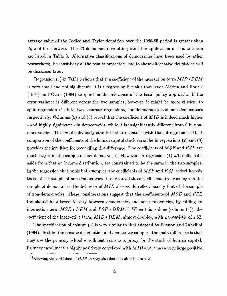
Regression (1) in Table 6 shows that the coefficient of the interaction term MID*DEM

is very small and not significant. It is a regression like this that leads Alesina and Rodrik

(1994) and Clark (1994) to question the relevance of the fiscal policy approach. If the

error variance is different across the two samples, however, it might be more efficient to

split regression (1) into two separate regressions, for democracies and non-democracies

respectively. Columns (2) and (3) reveal that the coefficient of MID is indeed much higher

- and highly significant - in democracies, while it is insignificantly different from 0 in non-

democracies. This result obviously stands in sharp contrast with that of regression (1). A

comparison of the coefficients of the human capital stock variables in regressions (2) and (3)

provides the intuition for reconciling this difference. The coefficients of MSE and FSE are

much larger in the sample of non-democracies. However, in regression (1) all coefficients,

aside from that on income distribution, are constrained to be the same in the two samples.

In the regression that pools both samples, the coefficients of MSE and FSE reflect heavily

those of the sample of non-democracies. If one forced these coefficients to be so high in the

sample of democracies, the behavior of MID also would reflect heavily that of the sample

of non-democracies. These considerations suggest that the coefficients of MSE and FSE

too should be allowed to vary between democracies and non-democracies, by adding an

interaction term MSE * DEM and FSE * DEM.11 When this is done (column (4)), the

coefficient of the interactive term, MID * DEM, almost doubles, with a t-statistic of 1.52.

The specification of column (4) is very similar to that adopted by Persson and Tabellini

(1994). Besides the income distribution and democracy samples, the main difference is that

they use the primary school enrollment ratio as a proxy for the stock of human capital.

Primary enrollment is highly positively correlated with MID and it has a very large positive

11 Allowing the coefficient of GDP to vary also does not alter the results.

19

coefficient in a growth regression on a sample of non-democracies. MSE and FSE are also

highly positively correlated with MID, but their coefficients in a growth regression have

opposite signs. Therefore, the difference between democracies and non-democracies in the

effects of income distribution is larger when the flow, rather than the stock, of human

capital is controlled for. In fact, if the primary enrollment ratio were used instead of

MSE and FSE in column (4), the coefficient of MID * DEM would be .155, with a

t-statistic of 2.80. Based on this last specification, Persson and Tabellini argue strongly

in favor of the fiscal policy approach. As shown above, Alesina and Rodrik (1994) and

Clark (1994) reach the opposite conclusion on the basis of a specification like (1), again

with primary enrollment rather than educational attainment as the human capital variable.

The foregoing discussion shows that these differences can be explained in large part on the

basis of the different specifications adopted.

One problem that makes it difficult to interpret the results obtained so far is the high

correlation between the level of GDP per capita and the democracy dummy variable. Out

of 33 democracies, the only countries with a GDP per capita below the cut-off value of

$1,500 previously used to define poor countries are Botswana, India, Sri Lanka, Dominican

Republic, Malaysia, and Colombia. If one splits the sample of countries into rich and

poor, the results mimic those obtained when splitting the sample into democracies and

non-democracies. Regressions based on the distinction between rich and poor countries are

presented in Table 7; in column (4), which allows for the coefficients of the human capital

variables to differ in the two samples, the coefficient of the interactive term MID * RICH

is .190, with a t-statistic of 2.08. Regressions (2) and (3) also show that the coefficient

of MID is very high and significant in the sample of rich countries, and very low and

insignificant in the sample of poor countries. These results persist if the cut-off level of

GDP per capita is set at $1,000.

A lower coefficient of the income distribution variable in the sample of poor countries

could be rationalized in a number of ways. Empirically, this is the result one should expect if

measurement error problems are more serious in poor countries. Theoretically, as discussed

in footnote 3 several models have the implication that, at low levels of income, equality

20

might be less good for growth than at high levels of income, essentially because starting

the process of development might require concentrating the little resources available in a

relatively small group. Other possible explanations of the difference between poor and

rich countries will be discussed later. But the basic point is simple: assuming they are

robust, it is not clear whether the regularities highlighted in Table 6 can be attributed to

a democracy effect rather than to an income effect.

In addition, the democracy effect does not appear to be robust. If one were to conduct

a robustness analysis on the coefficient of MID*DEM in regression (4) of Table 6, similar

to the analysis of Table 5, the results would be rather disappointing. For instance, the

exclusion of Venezuela alone causes the estimated coefficient of MID * DEM to fall to

.088, with a t-statistic of only (.98). The coefficient also falls to .084 (t-statistic: .97)

when the 5 countries with slowest growth are excluded, and to .064 (t-statistic: .70) in the

WLS regression. Finally, the Krasker-Welsch robust estimate, .087 (t-statistic: .84) is also

considerably lower than the OLS estimate.

4.5 The role of different samples.

Besides specification, existing empirical studies on income distribution and growth differ

along two other dimensions: the income distribution data and the definition of democracy.

Persson and Tabellini define a democracy as a country that was a democracy according to

Jodice and Taylor (1983) and Bank (1987) for more than 75% of the time. The definition

adopted by Alesina and Rodrik is similar to mine, and is also based on Jodice and Taylor

(1988). Gastil ranks countries in terms of "political rights" on a scale from 1 (the most

democratic) to 7. This is the index used inbarro (1994). A dicothomous criterion based on

the Gastil index could be to define a democracy as a country with an average value of the

Gastil index between 1973 and 1985 (as reported in the Barro and Lee dataset) less than or

equal to 3. Table 3 presents the samples of democracies based on the Persson and Tabellini

definition and the Gastil index. Note that while the differences between the Gastil index

and mine are very minor, the differences between the Persson-Tabellini index and mine are

much more substantial. In particular, the former includes in the group of democracies the

21

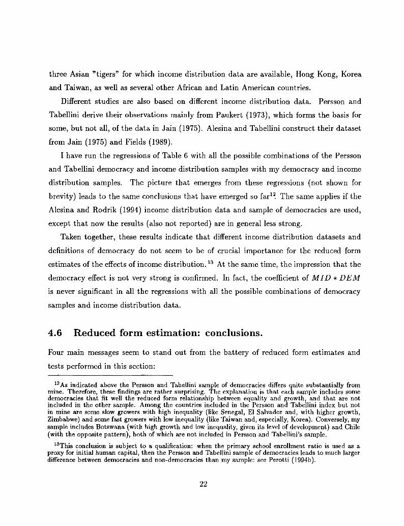
three Asian "tigers" for which income distribution data are available, Hong Kong, Korea

and Taiwan, as well as several other African and Latin American countries.

Different studies are also based on different income distribution data. Persson and

Tabellini derive their observations mainly from Paukert (1973), which forms the basis for

some, but not all, of the data in Jain (1975). Alesina and Tabellini construct their dataset

from Jain (1975) and Fields (1989).

I have run the regressions of Table 6 with all the possible combinations of the Persson

and Tabellini democracy and income distribution samples with my democracy and income

distribution samples. The picture that emerges from these regressions (not shown for

brevity) leads to the same conclusions that have emerged so far12. The same applies if the

Alesina and Rodrik (1994) income distribution data and sample of democracies are used,

except that now the results (also not reported) are in general less strong.

Taken together, these results indicate that different income distribution datasets and

definitions of democracy do not seem to be of crucial importance for the reduced form

estimates of the effects of income distribution.13 At the same time, the impression that the

democracy effect is not very strong is confirmed. In fact, the coefficient of MID * DEM

is never significant in all the regressions with all the possible combinations of democracy

samples and income distribution data.

4.6 Reduced form estimation: conclusions.

Four main messages seem to stand out from the battery of reduced form estimates and

tests performed in this section:

12 As indicated above the Persson and Tabellini sample of democracies differs quite substantially frommine. Therefore, these findings are rather surprising. The explanation is that each sample includes somedemocracies that fit well the reduced form relationship between equality and growth, and that are notincluded in the other sample. Among the countries included in the Persson and Tabellini index but notin mine are some slow growers with high inequality (like Senegal, El Salvador and, with higher growth,Zimbabwe) and some fast growers with low inequality (like Taiwan and, especially, Korea). Conversely, mysample includes Botswana (with high growth and low inequality, given its level of development) and Chile(with the opposite pattern), both of which are not included in Persson and Tabellini's sample.

13This conclusion is subject to a qualification: when the primary school enrollment ratio is used as aproxy for initial human capital, then the Persson and Tabellini sample of democracies leads to much largerdifference between democracies and non-democracies than my sample: see Perotti (1994b).

22

(1) There is a positive association between equality and growth, although a good deal of it

is coming from intercontinental variation;

(2) This positive association is quantitatively much weaker, and statistically insignifi-

cant, for poor countries; however, this can be explained both on empirical and theoretical

grounds;

(3) There is some indication that the association between equality and growth is stronger

in democracies; however, the democracy effect does not seem to be very robust;

(4) Because of the high concentration of democracies in rich countries, it is virtually impos-

sible to distinguish an income effect from a democracy effect in the relationship between

income distribution and growth.

5 The fiscal policy approach.

This section begins the analysis of the various approaches that lead to the reduced form

studied so far. Since the different explanations are not necessarily mutually exclusive,

ideally one should estimate the specific channels and their interactions. However, taken

literally this approach would require dealing with several endogenous variables at a time,

and therefore would require estimating large systems with many parameters and interactive

terms. There is no hope of achieving meaningful estimates of such systems with the small

cross-section of income distribution data currently available. Hence, the strategy followed

here consists in estimating different simple models, each embodying one of the channels

surveyed above, and each consistent with the reduced forms estimated above.

Although the preliminary evidence on the fiscal policy approach, from the reduced form

estimates of the previous section, is mixed at best, it is still interesting to study whether at

least one of the two components can shed some light on our understanding of fiscal policy

and/or growth.

The first preliminary question is what is the appropriate fiscal variable to test the

fiscal policy approach. As the brief survey in section 2 showed, the link between income

distribution and growth in this approach is the pression for redistribution that arises in

23

highly unequal societies14. Hence, the first class of candidates includes those types of

government expenditure that are explicitly redistributive in nature: social security and

welfare, health and housing, and public expenditure on education. On the other hand,

in these models what matters for growth is the distortions caused by the taxation that

accompanies these redistributive expenditures. For instance, if taxation were lump-sum,

a redistributive fiscal policy would have no distortionary effects on growth, because the

marginal return to investment would not be affected1? Hence, the second class of candidates

includes measures of taxation, like the average marginal tax rate, the average tax on labor,

and the average personal income tax.16

I begin the test of the fiscal policy approach in Table 8 with estimates of the structural

model using the average marginal tax rate between 1970 and 1985 (MTAX) as the fiscal

policy variable. This measure has at least two advantages. First, relative to the other tax

variables, it has the dimension of a marginal, rather than an average, tax rate and therefore

it is conceptually the right measure of the distortionary effects of fiscal policy. Second, it

is particularly appropriate in the context of the fiscal policy approach because in these

models income distribution is an important determinant of the progressivity of the tax rate17

Each panel of Table 8 contains estimates of the two structural equations, the economic

mechanism (result FP1 in section 2) and the political mechanism (result FP2), with GR

and MTAX as the dependent variables, respectively. In the first two columns, the sample

14The working of the economic and political mechanisms was illustrated in section 2 for the case ofpurely redistributive expenditure. A similar logic also applies to the case of directly productive governmentexpenditure, as in Alesina and Rodrik (1994), although the mechanism is now slightly less straightforwardsince the negative growth effects of distortionary taxation must be weighed against the positive effects ofpublic investment.

15A possible exception to this statement would occur if expenditure had direct distortionary effects, forinstance because it distorts labor supply by increasing the reservation wage of unions. However, theseeffects are likely to be small compared to a direct tax effect.

16Like the expenditure variables, these variables come from Easterly and Rebelo (1993). Needless to say,all the expenditure and tax measures are far from perfect: see Easterly and Rebelo (1993) for a discussionof the problems involved.

17When taxes are linear and revenues are redistributed lump-sum, as in all the models surveyed in section2, the degree of progressivity is related one-to-one with the level of the tax rate. However, in more generalmodels, the two variables could be independent.

24

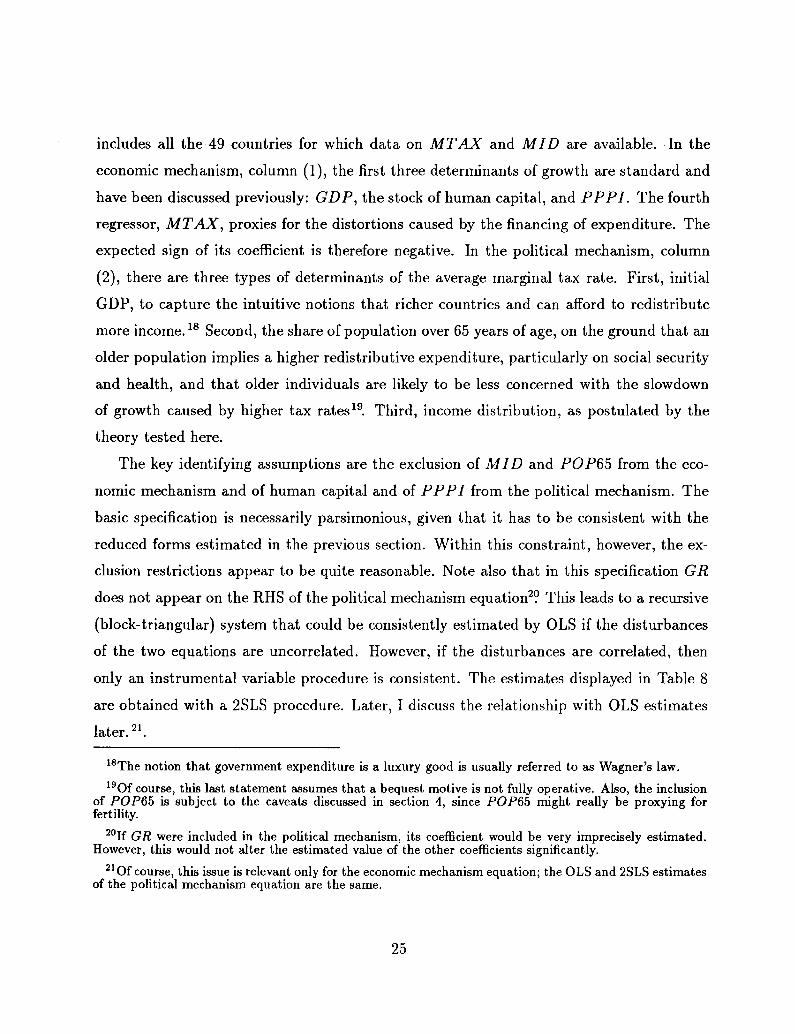
includes all the 49 countries for which data on MT AX and MID are available. In the

economic mechanism, column (1), the first three determinants of growth are standard and

have been discussed previously: GDP, the stock of human capital, and PPPI. The fourth

regressor, MT AX, proxies for the distortions caused by the financing of expenditure. The

expected sign of its coefficient is therefore negative. In the political mechanism, column

(2), there are three types of determinants of the average marginal tax rate. First, initial

GDP, to capture the intuitive notions that richer countries and can afford to redistribute

more income.18 Second, the share of population over 65 years of age, on the ground that an

older population implies a higher redistributive expenditure, particularly on social security

and health, and that older individuals are likely to be less concerned with the slowdown

of growth caused by higher tax rates19. Third, income distribution, as postulated by the

theory tested here.

The key identifying assumptions are the exclusion of MID and POP65 from the eco-

nomic mechanism and of human capital and of PPPI from the political mechanism. The

basic specification is necessarily parsimonious, given that it has to be consistent with the

reduced forms estimated in the previous section. Within this constraint, however, the ex-

clusion restrictions appear to be quite reasonable. Note also that in this specification GR

does not appear on the RHS of the political mechanism equation2? This leads to a recursive

(block-triangular) system that could be consistently estimated by OLS if the disturbances

of the two equations are uncorrelated. However, if the disturbances are correlated, then

only an instrumental variable procedure is consistent. The estimates displayed in Table 8

are obtained with a 2SLS procedure. Later, I discuss the relationship with OLS estimates

later.21.

18The notion that government expenditure is a luxury good is usually referred to as Wagner's law.19Of course, this last statement assumes that a bequest motive is not fully operative. Also, the inclusion

of POP6b is subject to the caveats discussed in section 4, since POP6b might really be proxying forfertility.

20If GR were included in the political mechanism, its coefficient would be very imprecisely estimated.However, this would not alter the estimated value of the other coefficients significantly.

21Of course, this issue is relevant only for the economic mechanism equation; the OLS and 2SLS estimatesof the political mechanism equation are the same.

25

In column (1) the coefficient of MTAX in the growth equation is positive, and highly

significant, rather than negative as the theory would predict. This finding, already noted

in reduced form regressions in Easterly and Rebelo (1993), is difficult to rationalize with

most of the existing theories, that emphasize the distortionary effects of government ex-

penditure and/or taxation. Note that these are all structural regressions: therefore, the

usual justification for the positive coefficient of fiscal variables in growth equations, namely

endogeneity, should not apply here.

In addition, in the political mechanism of column (2), income distribution plays es-

sentially no role. In itself, this last finding is not necessarily inconsistent with the fiscal

policy approach. An important prediction of this approach is that the pressure income

distribution exerts on government expenditure and taxation would be felt more strongly

in democracies. The relevant specification to test this theory would then include an in-

teractive term MID * DEM, as well as the dummy variable DEM. The theory would

predict that: (z) the coefficient of MID * DEM should be negative, and (ii) regardless

of what happens in non-democracies, the effect of an increase in equality on government

expenditure and the marginal tax rate should be negative in democracies, i.e. the sum of

the coefficients of MID and MID * DEM should be negative.

In fact, the point estimates of the new specification (columns (3) and (4)) are consistent

with both predictions2? In democracies, inequality does have a large effect on social security

expenditure, while in non-democracies this effect is essentially zero. However, the coefficient

on MID * DEM is not even close to significant. The picture is slightly more favourable

in columns (5) and (6), where the model is estimated on the sample of democracies only.

Now the coefficient of MID is very large in absolute value, -1.906, implying that, in this

sample, a ceteris paribus increase in the share of the middle class by 1% is associated with

a reduction in the average marginal tax rate by almost 2% on average. The t-statistic on

this coefficient also increases substantialy, to 1.42. Note, however, that in column (5) the

marginal tax rate is still positively, rather than negatively, associated with growth.

22This specification also includes the two interactive terms MSE * DEM and FSE * DEM, based onthe discussion in section 3.

26

POP65, as expected, has a positive, and very significant, coefficient. In addition,

if POP65 were omitted, MID would be insignificantly different from 0. The reason is

that POP65 is positively related both to equality and to taxation. This illustrates the

importance of controlling for demographic factors when testing for the effects of income

distribution on fiscal policy.

These patterns persist when other fiscal policy variables are used rather than the average

marginal tax rate, as in Table 9. For brevity, only estimates from regressions on the whole

sample, on a specification like in columns (3) and (4) in Table 8, are included in this last

table. In the first two lines of Table 9, I report 2SLS and OLS estimates of the fiscal

policy variable in the economic mechanism. A comparison of OLS and 2SLS estimates

is advisable because the instruments used for the fiscal policy variables in the economic

mechanism (MID and POP65) might not be very good ones.

In the economic mechanism all 6 variables have positive coefficients; the only insignif-

icant coefficients of the 2SLS estimates are those of public expenditure on education and,

marginally, of personal taxation. Also, these results persist in the OLS regressions, although

the size and the t-statistics of the estimated coefficients are generally lower. Therefore, not

only taxation, but also redistributive expenditures are positively associated with growth in

these structural regressions. Once again, these results are difficult to explain for virtually

any of the existing standard economic and political models of fiscal policy. For social se-

curity and welfare expenditure (the single most important expenditure item between those

employed here), these results can be explained in models where social security is a way to

convince less productive individuals to leave the labor force (as in Sala-I-Martin (1992)),

or it is part of an intergenerational contract that enhances social consensus and therefore

investment, as in Bellettini and Berti-Ceroni (1995), or where redistributive expenditure in

general is a way to overcome borrowing constraints and enable poor individuals to invest

in human capital, as in Perotti (1993).

An even more important message of this table is that there is also very little evidence of

a negative association between equality and fiscal variables in democracies. It is true that

in the political mechanism, MID * DEM has the expected negative sign in 4 cases out of

27

6, but social security and welfare is the only type of expenditure for which it is significant.

Notice that in the case of personal income taxation the coefficient of MID is significantly

positive.

Other robustness and sensitivity checks do not alter the two main messages of Table

8, namely the positive association between fiscal policy variables and growth and the very

weak - or even inexistent - negative relationship between equality and fiscal variables. To

conserve space, I will only discuss the main findings, without presenting the estimates

in separate tables. First, the results do not change appreciably when other definitions of

democracy or other income distribution datasets are used. Second, the results do not appear

to be sensitive to omitted variables and to outliers. An important aspect that has been

neglected so far is the role of cultural, religious and institutional factors in determining the

size of the social security system. Adding regional dummies to the list of regressors in the

political mechanism does not alter significantly the coefficients of the income distribution

variables. One might also argue that more urbanized societies have larger social security

systems, as both tax collection and the dispensing of subsidies is facilitated in an urban

environment. Indeed, urbanization has a positive coefficient in the political mechanism,

but again the income distribution coefficients do not change in any significant way. Finally,

dropping one observation at a time in the specification of columns (3) and (4) of Table 8

or estimating the system using an instrumental variable extension of the Krasker-Welsch

estimator also does not reveal any important outlier or group of outliers. Finally, like in

the case of the reduced form regressions, if one were to divide the countries into rich and

poor, rather than democracies and non-democracies, these two different ways to partition

the sample would give very similar results. Once again, it is very difficult to distinguish an

income effect from a democracy effect in this sample.

28

6 The political instability approach.

The basic intuition behind the socio-political instability approach, briefly presented in

section 2, is quite straightforward. 23In highly polarized societies, there are strong incentives

for the different groups to organize and engage in activities outside the market and outside

the usual channels of political representation in order to appropriate some of the resources

of the other groups. The resulting uncertainty on the final distribution of resources creates

disincentives to investment and growth.

To make this intuition operational, it is necessary to provide a measurable definition of

instability. Schematically, one can think of two types of definitions. The first one focuses on

executive instability, i.e. the frequency of government turnovers (see Alesina et al. (1992)).

The second type of definition emphasizes phenomena of social unrest, both violent and

non-violent, including those that do not find an expression in constitutional changes of

government. Included in this definition are phenomena like political assassinations, mass

demonstrations, political strikes, coups, etc. This second definition is closer to the idea

briefly outlined in Section 2. Undoubtedly, one could also think of reasons why income

distribution might affect executive turnover; however, in this case the link appears less

direct.

The next issue then is how to make the second definition operational. Hibbs (1973),

Venieris and Gupta (1983) and (1986), Gupta (1990), and Alesina and Perotti (1995) con-

struct indices of socio-political instability by combining several indicators of social unrest

using the method of the principal components. The index that will be used here is derived

from Alesina and Perotti (1995). 24 The Alesina and Perotti index includes four proxies

of social unrest, all from Jodice and Taylor (1988): political assassinations (ASSASS),

violent deaths per million population (DEATH), successful coups (SCOUP), and unsuc-

cessful coups (UCOUP). The rationale for the inclusion of these variables is quite obvious;

also, the results do not change much if other available proxies of social unrest, like the

23The first part of this section is based heavily on Alesina and Perotti (1995).24As shown below, the results do not change appreciably if the Venieris and Gupta index is used.

29

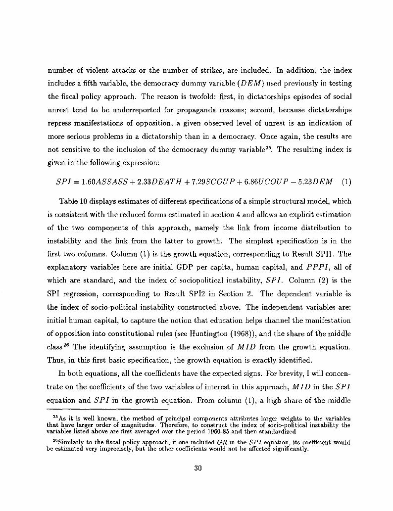
number of violent attacks or the number of strikes, are included. In addition, the index

includes a fifth variable, the democracy dummy variable (DEM) used previously in testing

the fiscal policy approach. The reason is twofold: first, in dictatorships episodes of social

unrest tend to be underreported for propaganda reasons; second, because dictatorships

repress manifestations of opposition, a given observed level of unrest is an indication of

more serious problems in a dictatorship than in a democracy. Once again, the results are

not sensitive to the inclusion of the democracy dummy variable25. The resulting index is

given in the following expression:

SPI = 1.60 ASS ASS + 2MDEATH + 7.29SCOUP + 6.86UCOUP - 5.23DEM (1)

Table 10 displays estimates of different specifications of a simple structural model, which

is consistent with the reduced forms estimated in section 4 and allows an explicit estimation

of the two components of this approach, namely the link from income distribution to

instability and the link from the latter to growth. The simplest specification is in the

first two columns. Column (1) is the growth equation, corresponding to Result SPI1. The

explanatory variables here are initial GDP per capita, human capital, and PPPI, all of

which are standard, and the index of sociopolitical instability, SPI. Column (2) is the

SPI regression, corresponding to Result SPI2 in Section 2. The dependent variable is

the index of socio-political instability constructed above. The independent variables are:

initial human capital, to capture the notion that education helps channel the manifestation

of opposition into constitutional rules (see Huntington (1968)), and the share of the middle

class26 The identifying assumption is the exclusion of MID from the growth equation.

Thus, in this first basic specification, the growth equation is exactly identified.

In both equations, all the coefficients have the expected signs. For brevity, I will concen-

trate on the coefficients of the two variables of interest in this approach, MID in the SPI

equation and SPI in the growth equation. From column (1), a high share of the middle

25 As it is well known, the method of principal components attributes larger weights to the variablesthat have larger order of magnitudes. Therefore, to construct the index of socio-political instability thevariables listed above are first averaged over the period 1960-85 and then standardized

26Similarly to the fiscal policy approach, if one included GR in the SPI equation, its coefficient wouldbe estimated very imprecisely, but the other coefficients would not be affected significantly.

30

class is associated with low political instability, and from column (2) the latter is associated

with high growth.The effects implied by the estimates of their coefficients are definitely not

negligible: an increase in the share of the middle class by one standard deviation decreases

SPI by slightly more than half its standard deviation; in turn, this leads to an increase in

the annual rate of growth of GDP by 1.1%.

The next panels of Table 10 show that these results are not sensitive to alternative

specifications of the model. One may argue that socio-political instability is highly influ-

enced by cultural factors. The inclusion of regional dummy variables (columns (3) and (4))

does not alter the basic picture: as expected, the coefficient of MID falls, although its

t-statistic does not. In columns (5) and (6), the regressors of the SPI equation include a

new variable, HOMOG, that represents the percentage of the population belonging to the

main ethnic or linguistic group (see Canning and Fay (1993)). Thus, this variable captures

the degree of fragmentation of the society, which is likely to be an important determinant

of socio-political instability. As one can see, the results are virtually unaffected27. In the

last two columns, the index of socio-political instability is from Gupta (1990), which is

estimated on a larger sample of countries (about 100), uses different variables, and is based

on the discriminant analysis rather than the principal component method. The results are

surprisingly close to those obtained before. An increase in the share of the middle class by

one standard deviation is associated with a fall in the index of about 1/3 of its standard

deviation, which in turn is associated with an increase in growth by about .8%.

In principle, one could also imagine a host of reasons why the level of GDP per capita

might be an important determinant of socio-political instability. However, the inclusion of

GDP in the SPI equation (not shown) does not change any of the coefficients of interest.

Also, a long tradition in economics, going back at least to Kaldor (1956), has argued that

the (functional) distribution of income is an important determinant of investment and

growth, since capitalists and workers have different propensities to save. However, when

27Virtualy identical results obtain when the index of ethnolinguistic fractionalization of Mauro (1995)is used instead of HQMOG. The difference between the two. indices is that the Mauro index takes intoaccount not only the largest group, but all ethnic and linguistic groups in a country: formally, it measuresthe probability that two randomly selected persons belong to two different groups.

31

MID is included in the growth equation directly (also not shown), its coefficient is not

significant, and the coefficient of MID in the SPI equation is not affected.

The results presented so far do not change significantly when the system is estimated

by dropping one observation at a time, and by applying the Krasker-Welsch 2SLS robust

estimator. However, these robust estimators might fail to detect the influence of groups of

countries with extreme values of certain important variables. This could be a particularly

serious problem here, because the distribution of the SPI index has a very fat left tail and

a very thin but long right tail. In fact, notice from Table 3 that most rich countries have

very low values of the SPI index, clustered around the minimum possible value of -.012. By

contrast, there are only 8 countries with a value of the index that exceeds the average by

more than 1 standard deviation. Thus, one might suspect that the results obtained so far

might be due to these few very unstable countries, that in many cases have also relatively

slow growth rates and quite unequal distributions of income.

To check for this possibility, Table 11 reestimates the model excluding countries with

extreme values of several variables. For brevity, only the coefficient of MID in the SPI

equation and of SPI in the growth equation are reported. For the latter coefficients, the

table presents both the 2SLS and the OLS estimates. This might be particularly important

in this context, and for a rather subtle reason. In the specification adopted, SPI in the

growth equation is instrumented by MID. In some cases, as countries with very large

values of the SPI index are excluded, the SPI index might not have much variation, as

it was argued above. As a result, MID might be a very poor instrument, and the second

stage regression might be subject to a large multicollinearity problem. The 2SLS estimate

of the coefficient of SPI in the growth equation might therefore be very unstable and

imprecise.

As a reference, column (1) presents estimates based on the whole sample, in a specifi-

cation like columns (1) and (2) of Table 10. Column (2) excludes countries with a value of

the SPI index more than 1.5 standard deviations above the average. The 2SLS estimate

of the SPI coefficient becomes extremely imprecise, as implied by the argument devel-

oped above; by contrast, the OLS estimate falls only slightly. The coefficient of MID in

32

the SPI equation falls, but remains significant. Column (3) excludes countries with very

unequal income distribution, corresponding to a share of the middle class more than 1.5

standard deviations below the mean. This clearly does not affect the point estimates of the

coefficients of interest. Columns (4), (5) and (6) clearly show that, as usual, the estimated

relationship is much stronger in rich countries.

Based on the results of the previous sections, one might legitimately ask whether the

regressions of this section would be different in democracies and non-democracies. One

might argue that in highly polarized and unstable societies one of the groups is more

likely to seize power and install a dictatorship as a way to protect its interests. Under

this explanation, democracies would grow faster exactly because they tend to be the less

polarized and unstable countries. Columns (7), (8) and (9) show that there is no appreciable

difference between democracies and non-democracies in the effects of income distribution

on political instability, although now the coefficients of MID are very low and imprecisely

estimated in both samples.28

7 The imperfect capital market and endogenous fer-

tility approaches.

In both the imperfect capital market and the endogenous fertility approach, the relevant

human capital investment decision is likely to be secondary school enrollment. The direct

costs of both primary and secondary schooling are very low virtually everywhere, since sec-

ondary education is practically free, or heavily subsidized, in most countries of the sample,

including developing countries. However, the opportunity costs of secondary education are

much higher, particularly in developing countries, than those of primary education. Pri-

mary education is also compulsory in practically all countries, while the same is not true

for secondary education, particularly at the beginning of the sample; moreover, the level

28Note that, if one tried to estimate the system with 2SLS on the sample of democracies and non-democracies separately, the estimate of the SPI coefficient would be very imprecise, due to the littlevariation in SPI in the sample of democracies. For this reason, only OLS estimates are presented in Table

33

of enforcement is much lower in the case of secondary education.

Table 12 begins the investigation of these two approaches29. I first estimate a two-

equation system with growth and fertility (FERT) as the endogenous variables. Following

Barro and Sala-I-Martin (1995), the measure of fertility employed here is the average of the

1965 and 1985 values of this variable. The first two columns of the table present the 2SLS

and OLS estimates of the growth regression, respectively. As expected, fertility has a large

and highly significant negative coefficient in the growth regression. This confirms results

obtained by, among others, Barro (1991), Barro and Sala-I-Martin (1995), and Galor and

Zang (1993). In addition, the 2SLS and OLS estimates of this equation are very similar.

For this reason, and to conserve space, when I perform some sensitivity analysis on the

fertility regression, I will not report the corresponding estimates of the growth regression.

In column (3), fertility depends on initial GDP, on educational attainment, and on

MID. Consistent with the discussion of section 2, the coefficient of MID is negative,

very large in absolute values, and higly significant. An increase in the share of the middle

class by one standard deviation is associated with a fall in fertility by .5 surviving child

per woman. The other coefficients also have the expected sign, with the usual exception

of female educational attainment: a higher female educational attainment is associated

with a higher fertility rate. This finding seems hard to explain for any reasonable theory

of fertility. More than anything, it probably indicates that the measure of educational

attainment used so far suffers from high measurement error. In fact, if one also controls for

both male and female secondary school enrollment ratios (MSEC and FSEC, respectively)

in the fertility regression, as in column (4), the coefficients of these last two variables are

eminently reasonable: that of male secondary enrollment ratio is insignificantly different

from zero, while that of female secondary enrollment ratio is negative and highly significant.

Note that controlling for female secondary enrollment causes the coefficient of MID to

fall by about 40%; this is not surprising, since according to the endogenous fertility aproach,

secondary school enrollment should be negatively correlated with fertility, and positively

29It is clear that the relevant concept in these two approaches is the distribution of wealth, rather thanincome. Because the former is available for very few countries, I will continue to use the latter in theempirical analysis that follows.

34

with growth. Of course, this also implies that secondary school enrollment ratios are jointly

endogenous with fertility, an issue to which I will return shortly. Even more than in the

case of schooling, it is hard to ignore cultural factors as determinants of fertility. Column

(5) includes regional dummies for Latin America, Africa and Asia: all their coefficients are

positive, as expected; also as expected, the coefficient of MID declines slightly in size, but

remains significant30

Table 13 investigates the relationship between income distribution and secondary school

enrollment. I start with the female secondary enrollment ratio. As in Table 12, columns

(1) and (2) present the 2SLS and OLS estimates of the growth regression, where the rate of

growth between 1960 and 1985 depends on initial GDP per capita, PPPI and secondary

school enrollment. The predicted sign of this coefficient is obviously positive.

In column (3), secondary school enrollment depends on the level of GDP per capita

in 1960, on the usual measures of educational attainment, and on the share of the middle

class. The endogenous fertility approach would predict a positive coefficient on all three

types of variables. In richer countries and in countries with a higher stock of human capital,

for any given distribution of human capital the average return to education is higher and

therefore the investment in education is higher. Conversely, given the average stock of

human capital, a more equal distribution of it should imply that more individuals respond

to the higher return on education by investing in human capital.

These predictions are strongly supported by the estimates of columns (1) to (3). In

particular, in both columns (1) and (2), the coefficient of FSEC is positive and extremely

significant, although now it is twice as large in the 2SLS estimate than in the OLS estimate.

In column (3), the coefficient of MID is positive and significant. A difference in one

standard deviation of the share of the middle class is associated with a difference in female

secondary school enrollment ratio of about 6.5%. As usual, the only coefficient that turns

out with an unexpected sign is the female educational attainment measure.

Columns (4) to (6) present the same regressions as columns (1) to (3), except that now

30Life expectancy is also often used as an explanatory variable for fertility. In fact, when life expectancyis included among the regressors of the fertility equation, its coefficient turns out to be negative andsignificant; however, the coefficient of MID falls only slightly.

35

the second endogenous variable is male secondary school enrollment, rather that the female

one. Interestingly, the two sets of estimates are very similar. For this reason, from now on

I will present results pertaining to female secondary school enrollment only.

One could argue that secondary school enrollment is highly influenced by cultural factors

and other characteristics that are not likely to be picked up by the level of GDP per capita.

Column (7) adds continental dummies to the RHS of the regression of column (3); Sub-

Saharan countries do have significantly lower-than-average enrollment ratios, given their

GDP per capita, but the coefficient of MID is not significantly affected.

In column (8), I add fertility on the RHS of the previous regression. As discussed above,

in the endogenous fertility approach fertility and investment in education are two different

forms of investment, and are jointly determined. By comparing column (5) of Table 12 to

column (8) in this table, one can study the the interaction between fertility and investment

in education. The main findings can be summarized as follows. The coefficient of fertility

in the enrollment ratio regression of column (8) is negative and highly significant. Income

distribution retains almost no independent explanatory power. In the fertility equation

(column (5) of Table 12), as shown above the female enrollment ratio has a negative and

significant coefficient. The income distribution variable falls slightly when secondary school

enrollment is controlled for, but remains economically and statistically significant.

These findings are again largely consistent with plausible extensions of models of en-

dogenous fertility. In these models, the main source of variation in returns to investment in

schooling is the rate of fertility (see e.g. Becker, Murphy and Tamura (1989)). Therefore,

income distribution largely affects investment in education through its effects on the rate of

fertility. Once the rate of fertility is controlled for, one would expect a fall in the coefficient

of MID in the enrollment regressions. However, even after controlling for investment in

human capital, MID still has a significant explanatory power for fertility. Thus, holding

constant the return to human capital investment, income distribution still affects other

determinants of fertility. For instance, if the time devoted to raising children increases

with human capital, but at decreasing rates, a redistribution of human capital to the poor

is likely to reduce the rate of fertility.

36

As discussed above, according to both approaches one should expect a weaker effect of

income distribution on primary school enrollment ratios. This is in fact the case: if sec-

ondary school enrollment were replaced by primary school enrollment in all the regressions

of Table 12, the estimated coefficient of MID in the primary school enrollment equation

would now be negative. The fit of the regressions (not reported to conserve space) also

drops drastically.

The evidence presented so far, particularly in Table 13, is also consistent with the

imperfect capital market approach. This approach too would predict a positive coefficient

on all three types of determinants of secondary school enrollment in columns (3) and (6).

In richer societies, given the distribution of income, fewer agents are so poor or have such a

low marginal utility that they cannot afford or do not want to send their children to school.

Conversely, given the average income of the economy, in more equal societies more agents

will be away from the corner and will be able to invest in their children's human capital.

In principle, however, there are more direct ways to test for the role of imperfect capital

market in the transmission of the effects of income distribution. If a measure of the degree

of imperfection in capital markets were available, one could interact it with the income

distribution variable and estimate its coefficient. One such measure is the loan-to-value

ratio for home mortgages, assembled by Jappelli and Pagano (1994). However, this measure

is available for only about 20 countries with income distribution data, and all of them

high-income countries. Perhaps not surprisingly, the coefficients of the income distribution

variable and of the interactive terms turn out to be insignificant. De Gregorio (1994)

and others use the ratio of domestic credit to GDP as a measure of the development of

credit markets. This variable is available for a slightly larger sample, but it is also a very

crude approximation to the concept of borrowing constraints. Again, regressions using this

variable gave inconclusive results.

One possible way to discriminate between the two approaches is to look at how the

link between income distribution on one side and enrollment ratios and fertility on the

other varies with the level of development. Table 14, which displays only the coefficients

of interest in regressions for schooling and fertility, shows clearly that the coefficient of

37

income distribution is about twice as large in the sample of rich countries, both in the

enrollment ratio and in the fertility regression. As usual, a bigger measurement error

problem in poor countries is a possible cause of this result. However, this is also the result

that one would expect on the basis of a model like Becker, Murphy and Tamura (1991).

In fact, its crucial feature is that the returns to education are low at low levels of human

capital. This is particularly true for poor individuals in poor countries. Therefore, in poor

countries a redistribution of human capital to poor individuals causes a fall in fertility (the

estimates of the previous table suggest that even in very poor countries the substitution

effect of an increase in human capital prevails over the income effect) but small movements

in investment in education. In richer countries, the returns to investment in education at

low levels of human capital are higher, and therefore both schooling and fertility are more

responsive to a redistribution of human capital.

A higher coefficient of the income distribution variable in rich economies is more difficult

to rationalize in the context of the imperfect capital market approach. One would expect

borrowing constraints to be more important in poor than in rich countries. Accordingly,

a redistribution of income to the poor would be more effective in relaxing borrowing con-

straints in a poor economy. On the other hand, the imperfect capital market approach does

offer an alternative explanation why equality might not have a positive impact on growth

in poor economies. As discussed in footnote 3, this would be the case if, for instance, there

are fixed costs of investment in human capital; only if wealth is relatively concentrated will

some individuals be able to start investing.

8 Conclusions.

More equal societies have lower fertility rates and higher rates of investment in education.

Both are reflected in higher rates of growth. Also, very unequal societies tend to be

politically and socially unstable, which is reflected in lower rates of investment and therefore

growth. Finally, the data do not support the idea that more equal societies, particularly

those with democratic institutions, grow faster because they generate less demands for

redistribution and therefore less distortions.

38

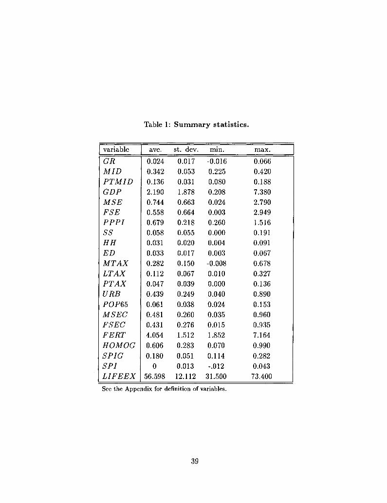
Table 1: Summary statistics.

variableGRMIDPTMIDGDPMSEFSEPPPISSHHEDMTAXLTAXPTAXURBPOP65MSECFSECFERTHOMOGSPIGSPILIFEEX

ave.

0.0240.3420.1362.1900.7440.5580.6790.0580.0310.0330.2820.1120.0470.4390.0610.4810.4314.0540.6060.180

056.598

st. dev.

0.0170.0530.0311.8780.6630.6640.2180.0550.0200.0170.1500.0670.0390.2490.0380.2600.2761.5120.2830.0510.01312.112

min.

-0.0160.2250.0800.2080.0240.0030.2600.0000.0040.003-0.0080.0100.0000.0400.0240.0350.0151.8520.0700.114-.012

31.500

max.

0.0660.4200.1887.3802.7902.9491.5160.1910.0910.0670.6780.3270.1360.8900.1530.9600.9357.1640.9900.2820.04373.400

See the Appendix for definition of variables.

39

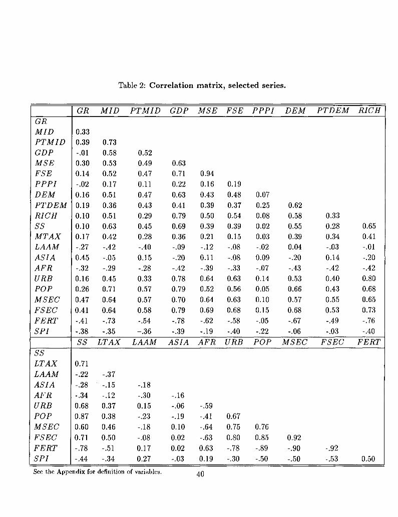
Table 2: Correlation matrix, selected series.

GRMIDPTMIDGDPMSEFSEPPPIDEMPTDEMRICHSSMTAXLAAMASIAAFRURBPOPMSECFSECFERTSPI

SSLTAXLAAMASIAAFRURBPOPMSECFSECFERTSPI

GR

0.330.39-.010.300.14-.020.160.190.100.100.17-.270.45-.320.160.260.470.41-.41-.38SS

0.71-.22-.28-.340.680.870.600.71-.78-.44

MID

0.730.580.530.520.170.510.360.510.630.42-.42-.05-.290.450.710.640.64-.73-.35

LTAX

-.37-.15-.120.370.380.460.50-.51-.34

PTMID

0.520.490.470.110.470.430.290.450.28-.400.15-.280.330.570.570.58-.54-.36

LAAM

-.18-.300.15-.23-.18-.080.170.27

GDP

0.630.710.220.630.410.790.690.36-.09-.20-.420.780.790.700.79-.78-.39

ASIA

-.16-.06-.190.100.020.02-.03

MSE

0.940.160.430.390.500.390.21-.120.11-.390.640.520.640.69-.62-.19

AFR

-.59-.41-.64-.630.630.19

FSE

0.190.480.370.540.390.15-.08-.08-.330.630.560.630.68-.58-.40

URB

0.670.750.80-.78-.30

PPPI

0.070.250.080.020.03-.020.09-.070.140.050.100.15-.05-.22

POP

0.760.85-.89-.50

DEM

0.620.580.550.390.04-.20-.430.530.660.570.68-.67-.06

MSEC

0.92-.90-.50

PTDEM

0.330.280.34-.030.14-.420.400.430.550.53-.49-.03

FSEC

-.92-.53

RICH

0.650.41-.01-.20-.420.800.680.650.73-.76-.40

FERT

0.50

See the Appendix for definition of variables. 40

Table 3: Detailed data, GDP, MID and SPI.

countryTanzaniaMalawiSier. Leo.NigerMyanmarTogoBangladeshKenyaBotswanaIndiaPakistanCongoBeninZimbabweSudanThailandKoreaZambiaHondurasSenegalTunisiaTaiwanPhilip.BoliviaDom. Rep.Sri LankaEl Salv.MalaysiaEcuadorPanamaTurkeyBrazilColombia

GDP0.2080.2370.2810.2840.3060.4150.4440.4700.4930.5330.5580.5630.5950.6150.6670.6880.690.7400.7480.7560.8520.8660.8740.8820.9560.9741.0621.1031.1431.2551.2551.3131.344

MID0.310.320.300.390.380.400.380.220.330.350.370.290.330.240.350.290.410.290.250.260.340.340.310.280.320.340.270.290.230.320.300.300.31

SPI-0.06-0.250.880.340.180.670.83-0.05-0.98-0.871.842.262.940.041.570.91NA

-0.210.49-0.12-0.08NA

-0.364.361.20

-0.870.80-1.061.910.290.53-0.01-0.46

dem.

PT

P,GP,PT,G

PTPT

PT

PT

PTPT

P,PT,GP,PT,G

PTP,PT,G

PTPT,G

P,PT,G

countryJamaicaGreeceCostaricaCyprusPeruHong KongBarbadosIranMexicoJapanSpainIraqIrelandS. AfricaIsraelChileArgentinaItalyUruguayAustriaFinlandFranceNetherlandU.K.NorwaySwedenAustraliaW. GermanyVenezuelaDenmarkN. ZealandCanadaSwitzerlandMJS.

GDP1.4721.4741.6631.6921.7211.7371.7471.8392.1572.2392.4252.5272.5452.6272.8382.9323.0913.2333.2713.9084.0734.4734.6904.9705.0015.1495.1825.2175.3085.4905.5716.0696.8347.380

MID0.300.370.280.410.300.350.370.300.310.390.380.270.400.360.400.310.330.380.380.420.400.350.390.400.400.420.410.380.310.420.390.410.420.41

SPI-1.030.20-1.190.210.74NA

-1.20-0.06-0.43-1.19-0.263.16-1.14-0.69-1.160.053.10-0.770.46-1.19-1.19-0.96-1.19-0.71-1.20-1.19-1.19-1.160.37-1.20-1.20-1.19-1.20-1.11

dem.P,PT,GP,PT,GP,PT,GP,PT,G

PTP,PT,G

P,PTP,PT,G

G

P,PT,G

P,PT,GP

P,PT,GP,PT

P,PT,GP,PT,GP,PT,GP,PT,GP,PT,GP,PT,GP,PT,GP,PT,GP,PT,GP,PT,GP,PT,GP,PT,GP,PT,GP,PT,GP,PT,G

See the Appendix for definition of variables,(various years), from Barro and Lee (1993)

"P": Perotti. "P-T": Persson and Tabellini (1994). "G": Gastil. Values of the SPI index are multiplied by 100.

Table 4: Reduced form regressions.

constant

GDP

MSE

FSE

PPPI

MID

LAAM

ASIA

AFR

URB

POP65

LIFEEX

nobsR2

(1)-.018

(-1.37)

-.002(-1.77)

.031(4.05)

-.025(-3.06)

-.002(-.30)

.118(2.84)

67.30

(2).003(.21)

-.003(-2.21)

.016(1.94)

-.011(-1.32)

-.004(-.48)

.082(1.81)

-.008(-1.71)

.011(1.59)

-.013(-2.48)

67.40

(3)-.018

(-1.31)

-.003(-1.48)

.028(3.44)

-.024(-2.79)

-.003(-.32)

.111(2.60)

008(.69)

64.26

(4)-.007(-.50)

-.006(-3.25)

.031(4.23)

-.024(-3.00)

.004(.45)

.047(1.02)

.241(2.82)

67.37

(5)-.049

(-3.43)

-.006(-3.87)

.021(2.94)

-.018(-2.36)

.0001(.016)

.083(2.14)

.0009(4.05)

65.45

Dependent variable: GR. t-statistics in parentheses. See the Ap-pendix for definition of variables.

42

Table 5: Reduced form regressions,robust estimators.

MID

nobs

(1). 136(3.19)Togo

66

(2).093(2.26)Venez.

66

(3).107(1.95)

59

(4).100(2.49)

62

(5).102(2.61)

62

(6).168(3.51)

58

(7).101(2.09)

67

(8).208(4.79)

67

(9).118(2.95)

67

Dependent variable: GR. t-statistics in parentheses. See the Appendix for definition of variables.In each columns, the coefficient of MID is estimated from a regression like (1) in Table 4. Column(1) reports the maximum value of the estimated coefficient in all the 67 regressions that leave outone country at a time. In parentheses the associated t-statistics and the country whose omissiongenerates the reported value of the coefficient. Column (2) reports the minimum value of theestimated coefficient, found in a similar way. In column (3), all countries with a value of MIDmore than 1.5 standard deviations below the average are excluded. In column (4), all countries witha growth rate more than 1.5 standard deviations above the average are excluded. In column (5),all countries with a growth rate more than 1.5 standard deviations below the average are excluded.In column (6), all countries with a per capita GDP in 1960 less than $500 are excluded. Column(7) reports the Krasker-Welsch robust estimates of the coefficient. Column (8) reports the WLSestimator. In column (9), the standard errors are corrected using the White heteroskedasticity-consistent estimator of the variance-covariance matrix.

43

Table 6: Reduced form, democracy effect.

sample

constant

GDP

MSE

FSE

PPPI

MID

MID * DEM

DEM

MSE * DEM

FSE * DEM

nobsR2

(1)all

-.008(-.50)

-.004(-2.35)

.032(4.20)

-.027(-3.24)

.0002(.02)

.178(1.51)

080(.88)

-.020(-.66)

67.31

(2)dem.

-.030(-1.13)

-.004(-2.55)

.009(.82)

-.008(-.73)

-.009(-.81)

.203(2.76)

33.27

(3)nondem.

-.016(-.95)

.0007(.17)

.042(3.37)

-.033(-1.50)

.015(1.21)

.050(.93)

34.43

(4)all

-.007(-.45)

-.004(-2.63)

.040(3.44)

-.026(-1.31)

.0004(.05)

.064(1.25)

.139(1.52)

-.029(-.97)

-.029(-1.76)

.015(.68)

67.35

Dependent variable: GR. t-statistics in parentheses.MID * DEM: MID interacted with the democracydummy variable. Similarly for MSE * DEM and FSE *DEM. See the Appendix for definition of other variables.

44

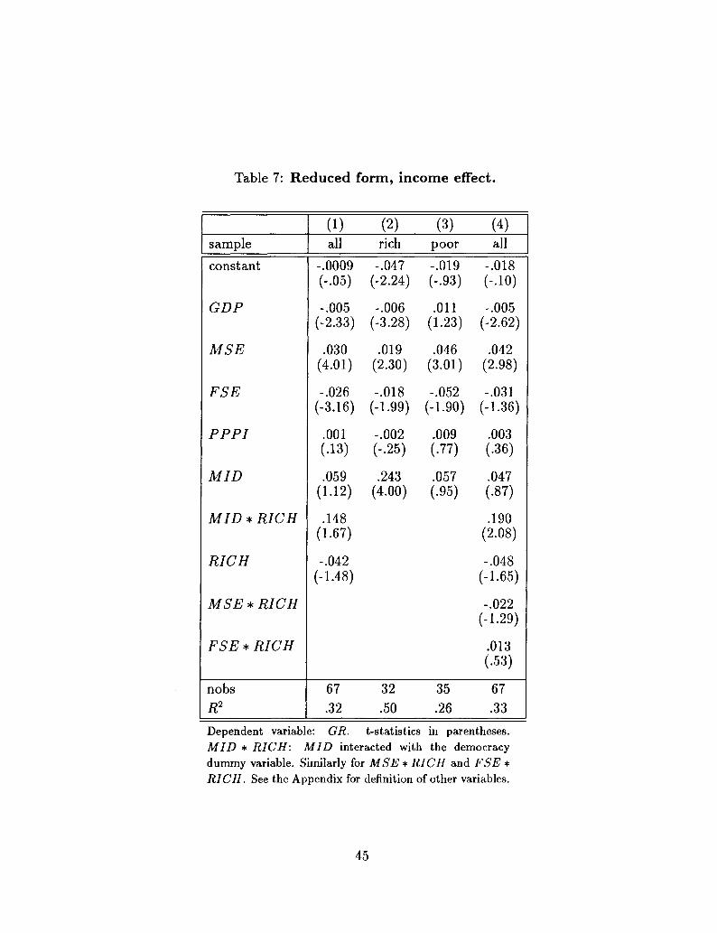
Table 7: Reduced form, income effect.

sample

constant

GDP

MSE

FSE

PPPI

MID

MID * RICH

RICH

MSE * RICH

FSE * RICH

nobsR2

(1)all

-.0009(-.05)

-.005(-2.33)

.030(4.01)

-.026(-3.16)

.001(.13)

.059(1.12)

.148(1.67)

-.042(-1.48)

67.32

(2)rich

-.047(-2.24)

-.006(-3.28)

.019(2.30)

-.018(-1.99)

-.002(-.25)

.243(4.00)

32.50

(3)poor

-.019(-.93)

.011(1.23)

.046(3.01)

-.052(-1.90)

.009(.77)

.057(.95)

35.26

(4)all

-.018(-.10)

-.005(-2.62)

.042(2.98)

-.031(-1.36)

.003(.36)

.047(.87)

.190(2.08)

-.048(-1.65)

-.022(-1.29)

.013(.53)

67.33

Dependent variable: GR. t-statistics in parentheses.MID * RICH: MID interacted with the democracydummy variable. Similarly for MSE * RICH and FSE *RICH. See the Appendix for definition of other variables.

45

Table 8: Economic and political mechanisms.

dep. var.sample

constant

GDP

MSE

FSE

PPPI

MTAX

MID

MID * DEM

DEM

POP65

nobsR2

(1)GR

.004(.47)

-.004(-2.39)

.004(.38)

.001(.10)

-.0005(-.07)

.090(3.61)

49.22

(2)MTAX

all

.164(1.13)

-.021(-1.50)

-.096(-.19)

3.047(3.78)

49.30

(3)GR

.005(.65)

-.002(-1.26)

.040(2.88)

-.046(-2.38)

.008(1.03)

.091(3.73)

49.24

(4)MTAX

all

.185(1.23)

-.022(-1.37)

-.222(-.45)

-.901(-.88)

.329(.99)

3.553(3.61)

49.29

(5)GR

(6)MTAX

dem.

.020(2.30)

-.002(-1.02)

-.020(-1.52)

.020(1.64)

-.016(-1.64)

.068(3.18)

27.30

.715(1.86)

-.020(-.98)

-1.906(-1.42)

4.430(3.28)

27.29

2SLS. t-statistics in parentheses. See the Appendix for definition of variables.

46

Table 9: Other fiscal policy variables.

ec.mech.,IV

ec.mech.,OLS

pol.mech.

nobs

FISC.POL.VAR.,

FISC.POL.VAR.

MID

MID * DEM

POP65

(4)MTAX

.090(3.73)

.014(.96)

-.222(-.45)

-.901(-.88)

3.553(3.61)

49

(5)LTAX

.246(3.07)

.83(2.08)

-.196(-.96)

-.137(-.41)

1.202(3.63)

50

(6)PTAX

.394(1.91)

.108(1.64)

-.069(-.47)

.504(2.09)

-.014(-.06)

48

(1)SS

.254(3.46)

.102(1.92)

-.005(-.41)

-.407(-1.98)

1.433(7.27)

54

(2)HH

.669(3.44)

.275(2.64)

-0.120(-1.57)

-0.029(-0.23)

0.406(3.25)

46

(3)ED

.200(.61)

.053(.40)

-0.134(-1.81)

0.103(0.81)

0.100(0.81)

47

The first two rows refer to the economic mechanism; the dependent variable is GR. Each entryin these two rows reports the 2SLS (first row) and OLS (second row) estimate of coefficient ofthe fiscal policy variable at the top of each column in a regression like (3) in Table 8. The lastthree rows refer to the political mechanism; the dependent variable is the fiscal policy variableat the top of each column. Each entry is the estimate of the coefficients of MID (third row),MID * DEM (fourth row), and POP65 (fifth row) in a regression like (4) in Table 8. MTAX:marginal tax rate; LTAX: labor taxation; PTAX: average personal income tax rate; SS: socialsecurity and welfare; HH: health and housing; ED: public expenditureon education. See theAppendix for definition of variables.

47

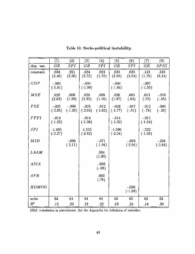
Table 10: Socio-political instability.

dep. var.

constant

GDP

MSE

FSE

PPPI

SPI

MID

LAAM

ASIA

AFR

HOMOG

nobsR2

(1)GR

.034(3.46)

-.004(-1.81)

.028(2.63)

-.025(-2.05)

-.014(-1.32)

-1.495(-2.27)

64.15

(2)SPI.021

(3.26)

.006(1.20)

-.009(-1.20)

-.090(-2.11)

64.23

(3)GR

.034(3.72)

-.004(-1.99)

.028(2.32)

-.025(-2.04)

-.014(-1.36)

-1.555(-2.82)

64.21

(4)SPI.023

(1.70)

.009(1.16)

-.012(-1.62)

-.071(-1.94)

.004(1.09)

-.006(-.08)

.003(.78)

64.22

(5)GR

.035(3.58)

-.004(-1.84)

.026(1.97)

-.024(-1.77)

-.014(-1.32)

-1.606(-2.54)

60.19

(6)SPI.035

(3.54)

.005(.63)

-.007(-.91)

-.093(-2.94)

-.006(-1.09)

60.24

(7)GR

.143(1.79)

-.007(-1.55)

.013(.72)

-.012(-.74)

-.015(-1.04)

-.532(-1.58)

63.14

(8)SPIG

.310(8.14)

-.016(-.55)

-.008(-.28)

-.334(-2.84)

63.30

2SLS. t-statistics in parentheses. See the Appendix for definition of variables.

48

Table 11: Socio-political instability,sensitivity and robustness.

SPI, IV

SPI, OLS

MID

MID * RICH

MID * DEM

nobs

(1)

-1.495(-2.64)

-.563(-3.73)

-.089(-2.90)

64

(2)

-3.346(-1.20)

-.471(-1.96)

-.050(-2.26)

60

(3)

-1.267(-2.47)

-.620(-4.05)

-.114(-3.19)

59

(4)

-1.640(-2.84)

-.570(-3.66)

-.019(-.46)

-.130(-2.00)

64

(5)

-1.598(-4.03)

-.882(-4.46)

-.150(-3.53)

31

(6)

-1.862(-.53)

-.303(-1.35)

-.019(-.41)

33

(7)

-2.193(-2.47)

-.651(-3.54)

.032(-.89)

.002(.04)

64

(8)

-.862(-2.09)

-.031(-1.02)

34

(9)

-.461(-2.10)

-.033(-.69)

31

The first two rows refer to the growth equation; the dependent variable is GR. Each entry in these two rows reportsthe 2SLS (first row) and OLS (second row) estimate of the coefficient of SPI in a regression like (1) in Table 10.The last three rows refer to the SPI equation. Each entry is the estimate of the coefficients of MID (third row),MID * RICH (fourth row), or MID * DEM (fifth row) in a regression like (2) in Table 10. Column (1) displaysestimates from the whole sample. In column (2), all countries with SPI index more than 1.5 standard deviationsabove the average are excluded. In column (3), all countries with a share of the middle class more than 1.5 standarddeviations below the average are excluded. Regression (4) is estimated on the whole sample, allowing for a differentcoefficient of MID in rich and poor countries. Regressions (5) and (6) are estimated on the sample of rich andpoor countries, respectively. Regression (7) is estimated on the whole sample, allowing for a different coefficient ofMID in democracies and non-democracies. Regressions (8) and (9) are estimated on the sample of democracies andnon-democracies, respectively.

49

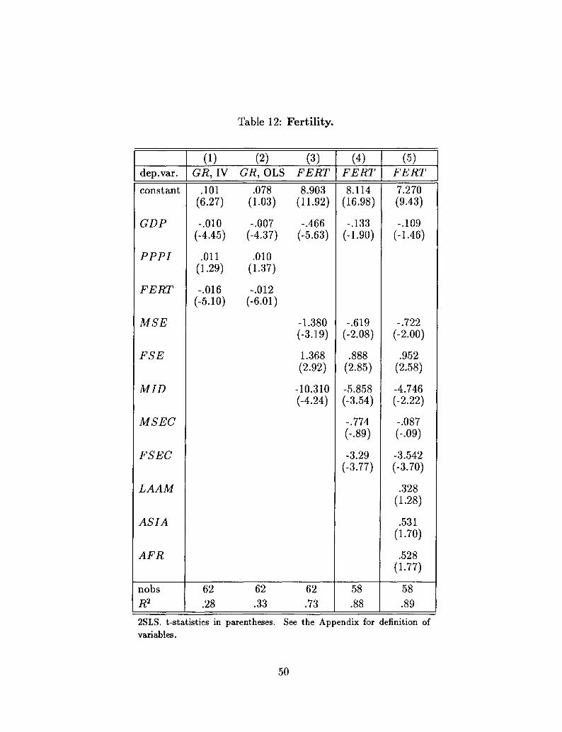
Table 12: Fertility.

dep.var.

constant

GDP

PPPI

FERT

MSE

FSE

MID

MSEC

FSEC

LAAM

ASIA

AFR

nobsR2

(1)GR, IV

.101(6.27)

-.010(-4.45)

.011(1.29)

-.016(-5.10)

62.28

(2)GR, OLS

.078(1.03)

-.007(-4.37)

.010(1.37)

-.012(-6.01)

62.33

(3)FERT8.903

(11.92)

-.466(-5.63)

-1.380(-3.19)

1.368(2.92)

-10.310(-4.24)

62.73

(4)FERT8.114

(16.98)

-.133(-1.90)

-.619(-2.08)

.888(2.85)

-5.858(-3.54)

-.774(-.89)

-3.29(-3.77)

58.88

(5)FERT7.270(9.43)

-.109(-1.46)

-.722(-2.00)

.952(2.58)

-4.746(-2.22)

-.087(-.09)

-3.542(-3.70)

.328(1.28)

.531(1.70)

.528(1.77)

58.89

2SLS. t-statistics in parentheses. See the Appendix for definition ofvariables.

50

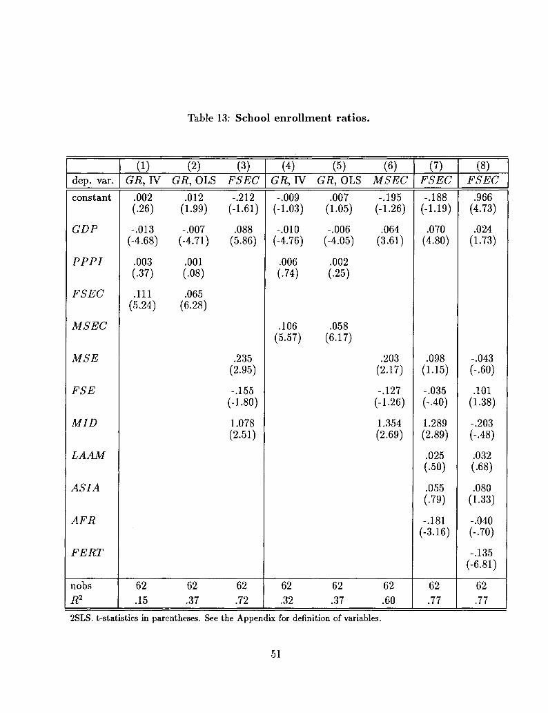
Table 13: School enrollment ratios.

dep. var.

constant

GDP

PPPI

FSEC

MSEC

MSE

FSE

MID

LAAM

ASIA

AFR

FERT

nobsR2

(1)GR,W

.002(.26)

-.013(-4.68)

.003(.37)

.111(5.24)

62.15

(2)GR, OLS

.012(1.99)

-.007(-4.71)

.001(.08)

.065(6.28)

62.37

(3)FSEC

-.212(-1.61)

.088(5.86)

.235(2.95)

-.155(-1.80)

1.078(2.51)

62.72

(4)GR, IV

-.009(-1.03)

-.010(-4.76)

.006(.74)

.106(5.57)

62.32

(5)GR, OLS

.007(1.05)

-.006(-4.05)

.002(.25)

.058(6.17)

62.37

(6)MSEC

-.195(-1.26)

.064(3.61)

.203(2.17)

-.127(-1.26)

1.354(2.69)

62.60

(7)FSEC-.188

(-1.19)

.070(4.80)

.098(1.15)

-.035(-.40)

1.289(2.89)

.025(.50)

.055(.79)

-.181(-3.16)

62.77

(8)FSEC

.966(4.73)

.024(1.73)

-.043(-.60)

.101(1.38)

-.203(-.48)

.032(.68)

.080(1.33)

-.040(-.70)

-.135(-6.81)

62.77

2SLS. t-statistics in parentheses. See the Appendix for definition of variables.

51

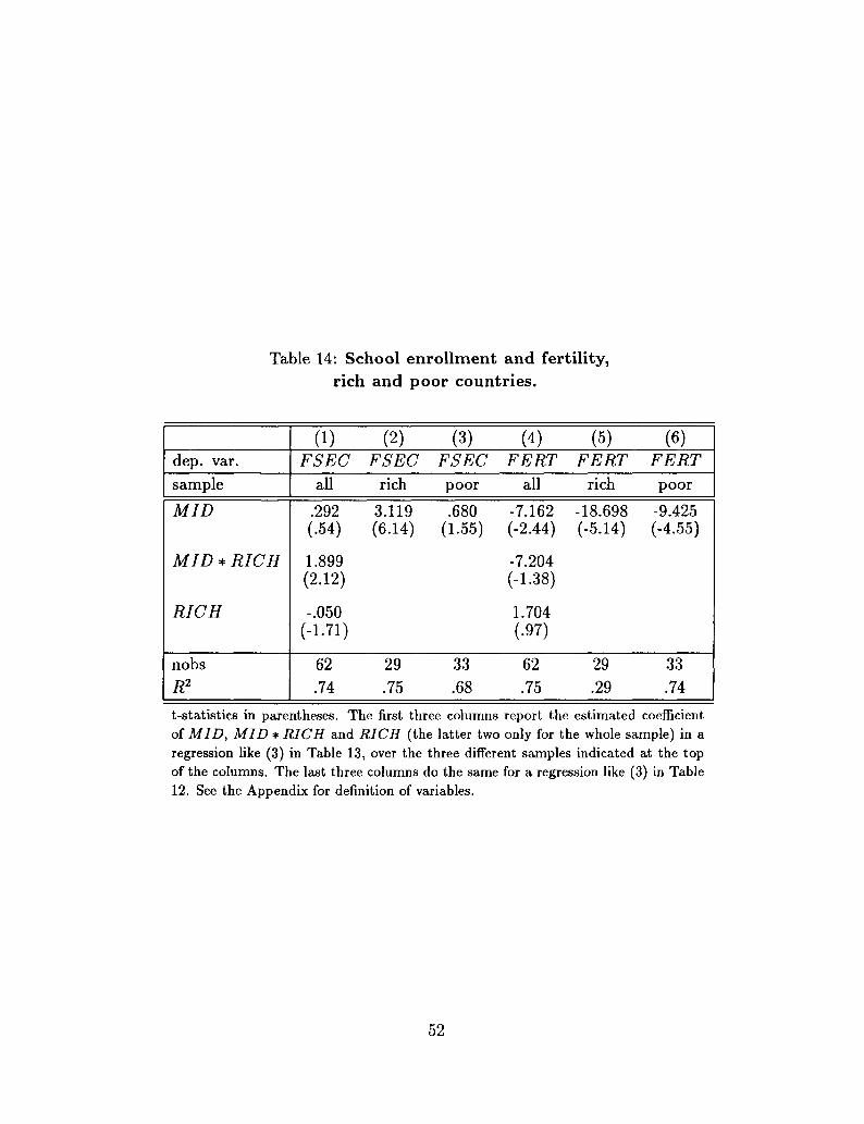
Table 14: School enrollment and fertility,rich and poor countries.

dep. var.

sample

MID

MID * RICH

RICH

nobs

R2

(1)FSEC

all

.292(.54)

1.899(2.12)

-.050(-1.71)

62

.74

(2)FSEC

rich

3.119(6.14)

29

.75

(3)FSEC

poor

.680(1.55)

33

.68

(4)FERT

all

-7.162(-2.44)

-7.204(-1.38)

1.704(.97)

62

.75

(5)FERT

rich

-18.698(-5.14)

29

.29

(6)FERT

poor

-9.425(-4.55)

33

.74

t-statistics in parentheses. The first three columns report the estimated coefficientof MID, MID * RICH and RICH (the latter two only for the whole sample) in aregression like (3) in Table 13, over the three different samples indicated at the topof the columns. The last three columns do the same for a regression like (3) in Table12. See the Appendix for definition of variables.

52

Data Appendix

This Appendix describes the data with their sources.

GR: average yearly growth rate of per capita GDP, 1960-85 (Barro-Lee (1994), henceforth:B-L).MID: share in income of the third and fourth quintiles, in or around 1960 (Perotti (1994b)).PTMID: share in income of the third quintile, in or around 1960 (Persson and Tabellini(1994)).GDP: per capita GDP in 1960 (B-L).MSE: average years of secondary schooling of the male population, 1960 (B-L).FSE: average years of secondary schooling of the female population, 1960 (B-L).PPPI: PPP value of the investment deflator, relative to the U.S., 1960 (B-L).SS: average share of government expenditure on social security and welfare in GDP, 1970-85 (Barro-Wolf (1991)).HH: average share of government expenditure on health and housing in GDP, 1970-88(Easterly-Rebelo (1993), henceforth: E-R).ED: average share of government expenditure on education in GDP, 1970-88 (E-R).MTAX: average marginal tax rate between 1970 and 1985, computed by Kormendi andKoster (1989) (E-R).LTAX: average share of labor taxation in GDP, 1970-88 (E-R).PTAX: average share of income taxes in personal income, 1970-88 (E-R).URB: urbanization rate in 1965 (World Bank).POP65: share of population over 65 years of age, average of 70, 75 and 85 values (B-L).MSEC: male secondary school enrollment ratio, average of 1965 and 1985 values (B-L).FSEC: female secondary school enrollment ratio, average of 1965 and 1985 values (B-L).FERT: net fertility rate (constructed as total fertility rate * (1 - infant mortality rate inthe first year of life)), average of 1965 and 1985 values (B-L).LIFE EX: life expectancy at birth in 1960 (B-L).HOMOG: percentage of the population belonging to the main ethnic or linguistic group(Canning ands Fay (1993)).SPI: index of socio-political instability, constructed as discussed in section 6.SPIG: index of socio-political instability, from Gupta (1990).DEM: democracy dummy variable, assigning a value of 1 to countries with an averagevalue over 1960 to 1985 of the democracy index in Jodice and Taylor (1988) larger than .5.PTDEM: democracy dummy variable, from Persson and Tabellini (1994).GDEM: democracy dummy variable, assigning a value of 1 to countries with a value ofthe Gastil index of political rights lower than or equal to 3 (B-L).

53

RICH dummy variable for countries with valuesof GDP higher than $1,500.AFR: dummy variable for Sub-Saharan countries (B-L).ASIA: dummy variable for South-Asian countries (B-L).LAAM: dummy variable for Latin American countries (B-L).

54

References

Aghion, P. and P. Bolton (1993): A Trickle-Down Theory of Growth and Developmentwith Debt Overhang, mimeo;Alesina, A., S. Ozler, N. Roubini, and P. Swagel (1992): Political Instability and EconomicGrowth, NBER working paper;Alesina, A. and R. Perotti (1995): Income Distribution, Political Instability, and Invest-ment, forthcoming, European Economic Review;Alesina, A. and R. Perotti (1994): The Political Economy of Growth: A Critical Survey ofthe Recent Literature, The World Bank Economic Review, 8, 351-71;Alesina, A. and D. Rodrik (1994): Distributive Politics and Economic Growth, QuarterlyJournal of Economics, 109, 465-90;Banerijee, A. and A. Newman (1991): Risk Bearing and the Theory of Income Distribu-tion, Review of Economic Studies, 58 211-35;Banerijee, A. and A. Newman (1993): Occupational Choice and the Process of Develop-ment, Journal of Political Economy, 101(2), 274-98;Banerijee, A. and A. Newman (1994): Poverty, Incentives, and Development, AmericanEconomic Review, Papers and Proceedings, 84(2), 211-15;Barro, R. J. (1991): Economic Growth in a Cross-Section of Countries, Quarterly Journalof Economics 106 407-44;Barro, R. J. (1994): Democracy and Growth, NBER working paper No. 4909;Barro, R. J. and G. S. Becker (1989): A Reformulation of the Economic Theory of Fertil-ity, Quarterly Journal of Economics, 103, 1-25;Barro, R. J. and J. Lee (1993): International Comparison of Educational Attainment, Jour-nal of Monetary Economics, 32(3), 363-94;Barro, R. J. and X. Sala-I-Martin (1995): Economic Growth, McGraw-Hills, New York;Becker, G. S., K. V. Murphy, and R. Tamura (1991): Human Capital, Fertility, and Eco-nomic Growth, Journal of Political Economy, 98(5), S12-37;Bellettini, G. and C. Berti-Ceroni (1995): Redistribution as a Social Contract, mimeo,Columbia University;Benhabib, J and A. Rustichini (1991): Social Conflict, Growth and Income Distribution,mimeo, New York University;Bertola, G. (1993): Market Structure and Income Distribution in Endogenous GrowthModels, American Economic Review, 83, 1184-99;Canning, D. and M. Fay (1993): Growth and Infrastructure, mimeo, Columbia University;Clark, B. R. G. (1994): More Evidence on Income Distribution and Growth, Journal ofDevelopment Economics;

55

De Gregorio, J. (1994): Liquidity Constraints, Human Capital Accumulation, and Growth,mimeo, International Monetary Fund;Easterly, W. and S. Rebelo (1993): Fiscal Policy and Growth, Journal of Monetary Eco-nomics, 32, 417-58;Fay, M. (1993): Illegal Activities and Income Distribution: a Model with Envy, mimeo,Columbia University;Fields, G. (1989): A Compendium of Data on Inequality and Poverty for the DevelopingWorld, mimeo, Cornell University;Galor, 0 . and H. Zang (1993): Fertility , Income Distribution and Economic Growth: The-ory and Cross-Country Evidence, mimeo, Brown University;Galor, 0 . and J. Zeira (1993): Income Distribution and Macroeconomics, Review of Eco-nomic Studies, 60, 35-52;Gupta, D. (1990): The Economics of Political Violence, Praeger, New York;Hibbs, D. (1973): Mass Political Violence: A Cross-Sectional Analysis, Wiley and Sons,New York;Huntington, S. (1968): Political Order in Changing Societies, Yale University Press, NewHaven;Jain, S. (1975): Size Distribution of Income: A Compilation of Data, World Bank, Wash-ington, D.C.;Jappelli, T. and M. Pagano (1994): Savings, Growth and Liquidity Constraints, QuarterlyJournal of Economics, 109, 83-110;Jodice, D. and D.L. Taylor (1988): World Handbook of Social and Political Indicators, YaleUniversity Press, New Haven;Kaldor, N. (1956): Alternative Theories of Distribution, Review of Economic Studies, 23,83-100;Krasker, W. S. and R. E. Welsch (1982): Efficient Bounded-Influence Regression Estima-tion, Journal of the American Statistical Association, 77 595-604;Krasker, W. S. , E. Kuh and R. E. Welsch (1982): Estimation with Dirty Data and FlawedModels, Ch. 11 in Griliches, Zvi and Michael Intrilligator: Handbook of Econometrics,North Holland, Amsterdam;Kuh, E. and R. E. Welsch (1980): Econometric Models and Their Assessment for Policy:Some New Diagnostics Applied to the Translog Energy Demand in Manufacturing, in S.Gass, ed.,: Proceedings of the Workshop on Validation and Assessment Issues of EnergyModels, National Bureau of Economic Standards, Washington, D.C., 445-475;Kuznets, S. (1955): Economic Growth and Income Inequality, American Economic Review,45, 1-28;Lecaillon, J. et al. (1984): Income Distribution and Economic Development, ILO, Geneva;

56

Mauro, P. (1995): Corruption and Growth, Quarterly Journal of Economics, 110, 681-712;Paukert, F. (1973): Income Distribution at Different levels of Development: A Survey ofEvidence, International Labor Review, 108, 97-125;Perotti, R. (1993): Political Equilibrium, Income Distribution, and Growth, Review of Eco-nomic Studies, 60, 755-776;Perotti, R. (1994a): Income Distribution and Investment, European Economic Review, 38,827-35;Perotti, R. (1994b): Income Distribution and Growth: An Empirical Investigation, mimeo,Columbia University;Persson, T. and G. Tabellini (1994): Is Inequality Harmful for Growth? Theory and Evi-dence, American Economic Review, 84(3), 600-21;Peters, S. C , A. M. Samarov and R. E. Welsch (1982): Computational Procedures for BoundedInfluence and Robust Regression, Technical Report No. 30, MIT Center for ComputationalResearch in Economics and Management Science;Sala-I-Martin, X. (1992): Transfers, NBER working paper No. 4186;Svensson, J. (1994): Investment, Property Rights and Political Instability: Theory andEvidence, mimeo, Institute for International Economic Studies, Stockholm;Tornell, A. and P. Lane (1994): Are Windfalls a Curse? A Non-Representative AgentModel of the Current Account and Fiscal Policy, mimeo, harvard University;Van Ginneken, W. and J. Park, eds. (1984): Generating Internationally Comparable In-come Distribution Estimates, ILO, Geneva;Venieris, Y. and D. Gupta (1983): Socio-Political Instability and Economic Dimensions ofDevelopment: A Cross-Sectional Model, Economic Development and Cultural Change, 31,727-56;Venieris, Y. and D. Gupta (1986): Income Distribution and Socio-Political Instability asDeterminants of Savings: A Cross-Sectional Model, Journal of Political Economy, 96, 873-83;

57

1994-1995 Discussion Paper SeriesDepartment of Economics

Columbia University1022 International Affairs Bldg.

420 West 118th StreetNew York, N.Y., 10027

The following papers are published in the 1994-95 Columbia University Discussion Paper serieswhich runs from early November to October 31 (Academic Year). Domestic orders for discussionpapers are available for purchase at $8.00 (US) each and $140.00 (US) for the series. Foreign orderscost $10.00 (US) for individual paper and $185.00 for the series. To order discussion papers, pleasesend your check or money order payable to Department of Economics, Columbia University to theabove address. Be sure to include the series number for the paper when you place an order.

708. Trade and Wages: Choosing among Alternative ExplanationsJagdish Bhagwati

709. Dynamics of Canadian Welfare ParticipationGarrey F. Barret, Michael I. Cragg

710. Much Ado About Nothing? Capital Market Reaction to Changes inAntitrust Precedent concerning Exclusive Territories.Sherry A. Glied, Randall S. Kroszner

711. The Cost of DiabetesMatthew Kahn

712. Evidence on Unobserved Polluter Abatement EffortMatthew E. Kahn

713. The Premium for Skills: Evidence from MexicoMichael Cragg

714. Measuring the Incentive to be HomelessMichael Cragg, Mario Epelaum

715. The WTO: What Next?Jagdish Bhagwati

716. Do Converters Facilitate the Transition to a New Incompatible Technology?A Dynamic Analysis of ConvertersJay Phil Choi

716A. Shock Therapy and After: Prospects for Russian ReformPadma Desai

717. Wealth Effects, Distribution and The Theory of Organization-Andrew F. Newman and Patrick Legros

1994-95 Discussion Paper Series

718. Trade and the Environment: Does Environmental Diversity Detract from the Case forFree Trade?-Jagdish Bhagwati and T.N. Srinivasan (Yale Univ)

719. US Trade Policy: Successes and Failures-Jagdish Bhagwati

720. Distribution of the Disinflation of Prices in 1990-91 Compared with Previous BusinessCycles-Philip Cagan

721. Consequences of Discretion in the Formation of Commodities Policy-John McLaren

722. The Provision of (Two-Way) Converters in the Transition Process to a New IncompatibleTechnology-Jay Pil Choi

723. Globalization, Sovereignty and Democracy-Jagdish Bhagwati

724. Preemptive R&D, Rent Dissipation and the "Leverage Theory"-Jay Pil Choi

725. The WTO's Agenda: Environment and Labour Standards, Competition Policy and theQuestion of Regionalism-Jagdish Bhagwati

726. US Trade Policy: The Infatuation with FT As-Jagdish Bhagwati

727. Democracy and Development: New Thinking on an Old Question-Jagdish Bhagwati

728. The AIDS Epidemic and Economic Policy Analysis-David E. Bloom, Ajay S. Mahal

729. Economics of the Generation and Management of Municipal Solid Waste-David E. Bloom, David N. Beede

730. Does the AIDS Epidemic Really Threaten Economic Growth?-David E. Bloom, Ajay S. Mahal

731. Big-City Governments-Brendan O'Flaherty

732. International Public Opinion on the Environment-David Bloom

1994-95 Discussion Paper Series

733. Is an Integrated Regional Labor Market Emerging in the East and Southeast Asia?-David Bloom, Waseem Noor

734. Migration, Integration and Development-Abhijit V. Banerjee, Andrew Newman

735. Infrastructure, Human Capital and International Trade-Ronald Findlay

736. Short Ballots: Why Mayors Are in Charge of So Many Different Things-Brendan O'Flaherty

737. Demand for Environmental Goods: Evidence from Voting Patterns on California Initiatives-Matthew Kahn and John Matsusaka

738. Inflation and Stabilization in Poland 1990 - 1995-S.Wellisz

739. Paniculate Pollution Trends in the 1980's-M. Kahn

740. Why has Wage Dispersion Grown in Mexico? Is it the Incidence of Reforms or theGrowing Demand for Skills?-M.I. Cragg and M. Epelbaum

741. Russia's Transition Toward the World Economy:-P. Desai

742. Poland: Transition and Integration in the World Economy-S. Wellisz

743. Team Effects on Compensation: An Application to Salary Determination in the National HockeyLeague-T. Idson and L.H. Kahane

744. Economic Development, Growth of Human Capital, and the Dynamics of the Wage Structure-J. Mincer

745. Technology Transfer with Moral Hazard-J.P. Choi (Oct.)

746. Risk Preference Smoothness and the APT-L.F. Herk, Columbia University, Institute on East Central Europe

747. A Characterization of Cointegration-P. Dhrymes (Oct.)

748. The Limiting Distribution of the Cointegration-P. Dhrymes (Oct.)

1994-95 Discussion Paper Series

749. A Useful Multivariate Stochastic Integration Result-P. Dhrymes (Oct.)

750. A Conformity Test for Cointegration-P. Dhrymes (Oct.)

751. Income Distribution, Political Instability, and Investment-R. Perotti (10/94)-A. Alesina

752. Capital Mobility and the (Inefficiency of Fiscal Unions-R. Perotti (12/94)

753. Income Disribution, Fiscal Policy and Delays in Stabilization-R. Perotti (6/95)

754. Fiscal Expansions and Adjustments in OECD Countries-R. Perotti (6/95)-A. Alesina

755. The Italian Budget Procedures: Analysis and Proposals-R. Perotti (5/95)-A. Alesino-M. Mare

756. Redistribution and Non-Consumption Smoothing in an Open Economy-R. Perotti (Sept.)

757. Growth, Income Distribution and Democracy: What the Data Say-R. Perotti (Sept.)