Growth drivers in emerging capitalist economies before and ...

Institute for International Political Economy Berlin

Growth drivers in emerging capitalist economies before and after the Global Financial Crisis

Author: Benjamin Jungmann

Working Paper, No. 172/2021

Editors: Sigrid Betzelt, Eckhard Hein (lead editor), Martina Metzger, Martina Sproll, Christina Teipen, Markus Wissen, Jennifer Pédussel Wu, Reingard Zimmer

Growth drivers in emerging capitalist economies before and after the Global Financial Crisis

Benjamin Jungmann

Berlin School of Economics and Law, Institute for International Political Economy (IPE)

Abstract: This paper contributes to the ongoing growth models (GMs) debate by investigating the

growth drivers of emerging capitalist economies (ECEs) in the periods before (2000-2008) and after

(2009-2019) the Global Financial Crisis (GFC). By drawing mostly on post-Keynesian economics, six

growth drivers are considered: Finance, i.e., household debt; changes in income distribution; price and

non-price competitiveness, as well as commodity prices; and finally, fiscal policy. By conducting cross-

country simple and multiple linear regressions to explain the growth of 19 ECEs in both periods, we

find that post-GFC growth was driven by non-price factors while price competitiveness played a role

in neither period. Likewise, commodity prices did not drive growth either. In terms of distribution, our

results indicate that cross-country growth was driven by rising income inequality in both periods; how-

ever, this relation lacks significance. In the post-crisis period, growth was associated with rising profit

shares. While this relation also lacks significance, it has to be assessed against various possibilities for

seemingly profit-led growth. Finally, with household debt accelerating and fiscal policy becoming more

expansionary after the crisis, our results indicate a potentially more prominent role for these factors

in driving post-crisis growth, however, this finding lacks robustness. We argue that the sparse robust

findings result from ECEs’ heterogeneity, particularly in terms of their growth models and subordinated

financialization.

Key words: growth model, growth driver, financialization, emerging capitalist economies, post-

Keynesian economics,

JEL codes: E11, E12, E65, F62, F65

Acknowledgements: This paper is a substantially revised and shortened version of my master thesis

submitted to the Berlin School of Economics and Law and the University Paris Sorbonne Nord. I am

most grateful for the comments, help and advice I received from Eckhard Hein, Ümit Akcay, Jonathan

Marie and the attendees of our research seminars. All errors are mine.

Benjamin Jungmann Berlin School of Economics and Law Badensche Str. 52 10825 Berlin e-mail: [email protected]

2

1 Introduction

Following the Global Financial Crisis (GFC) of 2007-09, the extreme divergence of growth models

(GMs)1 within developed capitalist economies (DCEs) that preceded it – debt-led on the one hand and

export-led on the other (Dodig et al., 2016) – has ceased to exist. Faced with the need for private

deleveraging, formerly debt-led economies have changed their GM: They have either become domes-

tic demand-led stabilized by public deficits as in the cases of the US and UK or rather export-led as in

the cases of Spain, Italy and Greece where demand compensation via public deficits was not possible

due to fiscal constraints and austerity policies (Hein et al., 2021). Commenced by Baccaro and Pontus-

son (2016), this GM-approach is now increasingly applied within the Comparative Political Economy

literature, thereby marking a shift within this discipline from New Consensus Macroeconomics with

supply-side determined long-run equilibria to the use of post-Keynesian based demand-focused ap-

proaches.2 Lately, scholars have attempted to extend the GM-approach to emerging capitalist econo-

mies (ECEs)3: Schedelik et al. (2021) link the work on the types of capitalism in ECEs to the respective

GMs of these countries. Types of capitalism assigned to ECEs range from ‘state-permeated capitalism’

(China and India), ‘dependent market economies’ (Central Eastern Europe), ‘patrimonial capitalism’

(Russia) and ‘hierarchical market economies’ (mostly in Latin America). Linking these types of capital-

ism with ECEs’ GMs, Schedelik et al. (2021) argue that ECEs might be able to switch their GM and

maintain their type of capitalism (China) while in other instances changes and ambiguities in the type

of capitalism are conducive to a change in the GM (Brazil). Focusing on the macroeconomic aspects,

Akcay et al. (2021) investigate eight large ECEs’ GMs before and after the GFC against the background

of their degree of financialization and distributional developments. While financialization has become

more entrenched in these ECEs after the GFC, distributional developments were rather heterogeneous.

In this setting, after the crisis, debt-led GMs have not ceased to exist among ECEs but rather prevailed

in Turkey and South Africa. Meanwhile, India has maintained its domestic demand-led GM character-

ized by current account and public deficits; Argentina and Brazil, both formerly export-led, have also

turned domestic demand-led; while China, though still export-led, saw a decrease in the relative im-

portance of its exports’ growth contribution. Thus, ECEs have not followed the post-GFC trajectory of

DCEs in abandoning debt-led GMs and turning more export-led, and have thus provided the necessary

1 Within the GM-approach, economies are classified according to their demand and financial resources by looking at the different demand components, their growth contributions and the sectoral financial balances. In some cases, the terms ‘demand regime’ or ‘macroeconomic regime’ are used (see for instance Akcay et al., 2021; Hein & Mundt, 2012). We will use these terms interchangeably. Irrespective of the term, the concept should not be confused with the distinction be-tween wage-led and profit-led demand that is going to be introduced in 2.2 and works at a different level of analysis. 2 For applications of the GM-approach within Comparative Political Economy see e.g. Hall (2018) and Johnston & Regan (2018). Stockhammer (2021) provides an overview on the post-Keynesian fundamentals of the GM-approach. 3 Generally, the term ECE refers to economies with a capitalist mode of production that feature some but not all of the characteristics of DCEs, e.g. in terms of financial and trade integration into world markets or sectoral composition of the economy.

3

counterpart to export-led DCE mercantilist economies with high current account surpluses by accept-

ing (rising) current account deficits. However, to some extent, DCEs and ECEs share a post-GFC orien-

tation towards domestic demand-led GMs stabilized by public deficits.

A different approach is applied by Kohler and Stockhammer (2021): Instead of classifying GMs

based on growth contributions, they investigate the relevance of four growth drivers, “which are fac-

tors that are hypothesized to cause changes in the components of aggregate income” (Kohler &

Stockhammer, 2021, p. 2) of 30 OECD countries before and after the GFC. Kohler and Stockhammer

consider finance in the form of household debt and housing prices, competitiveness in terms of price

and non-price factors and fiscal policy as possible growth drivers. In sum, their results suggest that: “(i)

house prices are a strong but cyclical driver of growth and thus periodically turn debt-led growth into

debt-driven stagnation; (ii) discretionary fiscal spending has become an important growth driver after

the GFC; and (iii) price competitiveness has failed to stimulate growth through foreign demand”

(Kohler & Stockhammer, 2021, p. 3). They maintain that the dichotomy of export-led versus consump-

tion-led GMs has lost its usefulness and the formerly debt-led GMs “underwent a debt- and austerity-

driven depression, whereas most previously export-led models failed to generate sustained growth

through exports” (2021, p.3).

Acknowledging the merit of looking into growth drivers, this paper seeks to deepen the under-

standing of the trajectories of ECEs after the GFC by applying the approach of Kohler and Stockhammer

(2021) to a sample of 19 ECEs.4 We seek to identify the growth drivers in these ECEs before and after

the GFC. To that end, we consider the drivers suggested by Kohler and Stockhammer (2021) taking into

account ECE specificities and adding two, namely, income distribution and commodity prices. First,

finance is considered by looking at household debt in ECEs in the context of their variegated (Kar-

wowski, 2020) and subordinated financialization (Kaltenbrunner & Painceira, 2018) amidst global fi-

nancial cycles (Rey, 2015). Second, in contrast to Kohler and Stockhammer (2021), we consider changes

in income distribution as a possible further driver based on the distinction between wage- and profit-

led demand in post-Keynesian economics (Bhaduri & Marglin, 1990). Income distribution relates to

finance as a growth driver as the increased debt-driven demand and growth characteristics of finan-

cialized economies compensate the loss in demand resulting from rising profit shares and increased

wage inequality in otherwise wage-led economies (Hein, 2014, Chapter 10) – which may then even

appear profit-led (Kapeller & Schütz, 2015). Truly profit-led economies, on the other hand, may foster

their growth via increased international price competitiveness, the third driver considered. Besides

fostering net exports, real depreciations are thought to be potentially able to enhance economic

4 The sample comprises countries that are commonly labelled as ECEs or similar. The selection was ultimately restricted by data availability, particularly in terms of financial indicators. Our sample encompasses the Latin American ECEs of Argen-tina, Brazil, Chile, Colombia and Mexico; the Asian ECEs of China, Indonesia, India, Korea, Malaysia and Thailand; the Central and Eastern European ECEs of the Czech Republic, Hungary, Poland and Russia; the Middle Eastern ECEs of Israel, Saudi Ara-bia and Turkey; and South Africa.

4

growth through increased activity in modern tradeable sectors and by averting overvalued exchange

rates (Rapetti, 2020). We further take into account non-price competitiveness, i.e. the technological

capabilities of a country that have been found to closely correspond to its income (Hidalgo & Haus-

mann, 2009), thereby, resonating with the reasoning based on Thirlwall's (1979) law and economic

structuralism (Ocampo & Parra, 2006). Fifth, we consider commodity prices as a further possible driver

for external demand and growth, particularly in the context of their latest ‘super cycle’ that started at

the onset of this century (Erten & Ocampo, 2013). Finally, fiscal policy is considered as a growth driver

which is said to be especially efficient in generating multiplier effects during economic slowdowns

(Gechert & Rannenberg, 2018). The role of fiscal policy is further assessed by making use of the litera-

ture on autonomous demand-driven growth (Allain, 2015). Following Kohler and Stockhammer (2021),

we assess the relevance of these growth drivers for the pre- and post-GFC period in a cross-country

analysis of 19 ECEs by comparing their bivariate correlations with national growth. Furthermore, mul-

tiple linear regressions are run to buttress the findings of the simple regressions. This methodology is

straightforward but comes with some caveats, particularly, it only at best establishes cross-country

correlations which do not necessarily constitute causalities while their absence may signify heteroge-

neity within the sample rather than the growth drivers’ insignificance for every country.

We see that ECEs grew slower after the GFC with a trend towards worsening current account bal-

ances. In terms of robust cross-country growth drivers, our results are sparse with the exception of

non-price competitiveness, which particularly drove growth in the post-crisis period whereas there are

no indications of price competitiveness and commodity prices driving growth in either period. The

absence of price competitiveness as a cross-country growth driver is particularly remarkable against

some indications of growth being accompanied by increasing income inequality during both periods

and with falling wage shares in the post-crisis years. Against the overall further entrenchment of finan-

cialization in ECEs in terms of rising household debt, there are indications that growth has in the post-

GFC period become more dependent on rising household debt, especially, in the years before 2014

when ECEs experienced pronounced capital inflows fuelled by loose US monetary policy. Similarly, fis-

cal policy turned more expansionary in these countries following the GFC but without becoming a ro-

bust cross-country growth driver. We argue that the absence of robust cross-country growth drivers

among ECEs reflects their heterogeneity, for instance, in terms of their ‘variegated’ financialization

(Karwowski, 2020) and GMs (Akcay et al., 2021). Thus, our mixed results emphasize the need of some

sort of classification beyond growth drivers.

The remainder is structured as follows: Section 2 reviews the literature on the six growth drivers.

Section 3 presents the descriptive data on the 19 ECEs and the conducted simple linear regressions.

Section 4 contains the econometric test of a multiple linear regression. Section 5 summarizes and dis-

cusses the results and relates them to the adjacent literature. Section 6 concludes.

5

2 Growth drivers: Finance, income distribution, competitiveness, commodity prices and fiscal policy

This section reviews six possible growth drivers. Whenever appropriate, ECE-specificities are taken into

account. First, finance is considered by looking at household debt in the ECEs considered in the context

of subordinate and variegated financialization within global financial cycles. Second, unlike Kohler and

Stockhammer (2021), we consider income distribution as a growth driver reviewing the distinction

between wage-led and (seemingly) profit-led demand. Third, the literature on price competitiveness

as a growth driver is reviewed while non-price competitiveness constitutes the fourth growth driver.

Fifth, in contrast to Kohler and Stockhammer (2021), we look at commodity prices and the super cycles

they follow. Finally, fiscal policy and its growth effects are considered through the literature on fiscal

multipliers and autonomous demand-driven growth.

2.1 Finance: Household debt, subordinate financialization and global financial cycles

Most broadly, financialization describes “the increasing role of financial motives, financial markets,

financial actors and financial institutions in the operation of the domestic and international economies”

(Epstein, 2005, p. 3). Macroeconomically, in DCEs, it has been associated with the emergence of ex-

port-led mercantilist and debt-led private demand boom GMs before the GFC, the latter characterized

by household indebtedness and current account deficits (Hein, 2014, Chapter 10). In between a do-

mestic demand-led GM has been found. In ECEs, debt-led GMs have been identified in Mexico before

the GFC (Hein & Mundt, 2012), in Turkey thereafter and in South Africa in both periods (Akcay et al.,

2021; Dodig et al., 2016). This, however, does not imply that financialization did not manifest in those

ECEs identified as export- or domestic demand-led. Instead, financialization among ECEs is variegated

in terms of dimensions and degrees (Karwowski, 2020). In the following, as Kohler and Stockhammer

(2021) do for DCEs, we will focus on the financialization, i.e. rising indebtedness, of households in ECEs

as a possible growth driver via increased private consumption and residential investment in the con-

text of their subordinate integration into global financial markets.5

In debt-led DCEs, fallen demand due to risen income inequality and decreased real investment has

been partly substituted by increased debt-financed household consumption and residential invest-

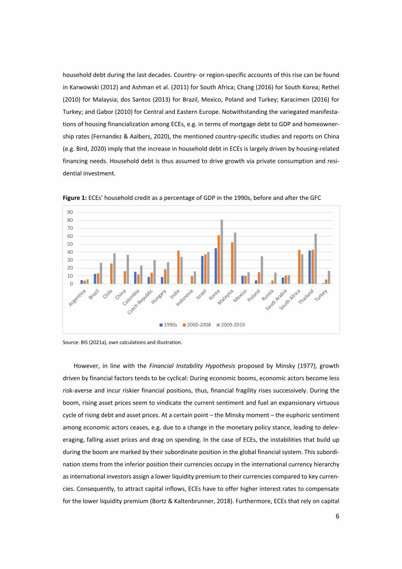
ment (Hein, 2014, Chapter 10). Figure 1 indicates that several ECEs have seen an increase in their

5 Financialization in ECEs is also associated with rising indebtedness of non-financial corporations (NFCs) (Karwowski & Stockhammer, 2017). In some cases, this rising indebtedness of NFCs is accompanied by rising investment, particularly, in real estate and infrastructure, as in Turkey (Orhangazi & Yeldan, 2021) or China (Chen & Kang, 2018). However, we do not consider it as a possible growth driver because the literature does suggest that rising NFC indebtedness also tends to be associated with heightened involvement of NFCs in financial activities (Demir, 2007, 2009; Akkemik & Özen, 2014; Correa et al., 2012; Farhi & Borghi, 2009), increased holding of liquid assets (Karwowski, 2012) and financial payouts (Kalinowski & Cho, 2009) at the expense of real investment.

6

household debt during the last decades. Country- or region-specific accounts of this rise can be found

in Karwowski (2012) and Ashman et al. (2011) for South Africa; Chang (2016) for South Korea; Rethel

(2010) for Malaysia; dos Santos (2013) for Brazil, Mexico, Poland and Turkey; Karacimen (2016) for

Turkey; and Gabor (2010) for Central and Eastern Europe. Notwithstanding the variegated manifesta-

tions of housing financialization among ECEs, e.g. in terms of mortgage debt to GDP and homeowner-

ship rates (Fernandez & Aalbers, 2020), the mentioned country-specific studies and reports on China

(e.g. Bird, 2020) imply that the increase in household debt in ECEs is largely driven by housing-related

financing needs. Household debt is thus assumed to drive growth via private consumption and resi-

dential investment.

Figure 1: ECEs’ household credit as a percentage of GDP in the 1990s, before and after the GFC

Source: BIS (2021a), own calculations and illustration.

However, in line with the Financial Instability Hypothesis proposed by Minsky (1977), growth

driven by financial factors tends to be cyclical: During economic booms, economic actors become less

risk-averse and incur riskier financial positions, thus, financial fragility rises successively. During the

boom, rising asset prices seem to vindicate the current sentiment and fuel an expansionary virtuous

cycle of rising debt and asset prices. At a certain point – the Minsky moment – the euphoric sentiment

among economic actors ceases, e.g. due to a change in the monetary policy stance, leading to delev-

eraging, falling asset prices and drag on spending. In the case of ECEs, the instabilities that build up

during the boom are marked by their subordinate position in the global financial system. This subordi-

nation stems from the inferior position their currencies occupy in the international currency hierarchy

as international investors assign a lower liquidity premium to their currencies compared to key curren-

cies. Consequently, to attract capital inflows, ECEs have to offer higher interest rates to compensate

for the lower liquidity premium (Bortz & Kaltenbrunner, 2018). Furthermore, ECEs that rely on capital

0102030405060708090

Argentin

aBraz

ilChile

China

Colombia

Czech Republic

Hungary

India

IndonesiaIsr

ael

Korea

Malaysi

a

Mexico

Poland

Russia

Saudi A

rabia

South Afric

a

Thaila

ndTu

rkey

1990s 2000-2008 2009-2019

7

inflows face the problem of their debt being of short maturity and denominated in foreign currency,

making them additionally vulnerable to exchange rate movements (Arestis & Glickman, 2002). Their

subordinate position is further reflected in the fact that capital flows to these countries largely depend

on the decisions of institutional investors in DCEs that are to a large extent determined by the liquidity

considerations of these investors and global factors, such as the monetary policy in DCEs (Bonizzi,

2017a). The respective cyclical and secular movement in capital flows, asset prices and credit growth

has become known as the global financial cycle (Rey, 2015). In this context, ECEs’ capital inflows are

linked to US monetary policy – increasing during expansionary and decreasing during restrictive mon-

etary policy stances (Bräuning & Ivashina, 2020; Ahmed & Zlate, 2014). The ‘taper tantrum’ of 2013,

when ECEs experienced widespread capital outflows following the US Federal Reserve’s announce-

ment of ending its quantitative easing (Akyüz, 2021), constitutes a prominent example of this mecha-

nism.

Country-specific accounts for the instabilities related to subordinate financialization have been

described for South Africa by Isaacs & Kaltenbrunner (2018) and for Brazil by Kaltenbrunner & Pain-

ceira (2015, 2018).6 Similarly, Orhangazi & Yeldan (2021) assert that the Turkish economic crisis of

2018 was the result of a GM dependent on foreign capital that fuelled domestic activity in the non-

tradable sector while manifesting import dependence and current account deficits due to real appre-

ciations. This constellation deteriorated the tradable sector and made Turkey vulnerable to a reversal

in capital inflows.

Summing up, we consider household debt as a growth driver fuelling private consumption and

residential investment. We expect it to exhibit cyclical characteristics amplified by the subordinate

position of ECEs in the global financial system.

2.2 Income distribution: Wage-led and (seemingly) profit-led demand

While not considered by Kohler and Stockhammer (2021), we review changes in the income distribu-

tion as a possible driver of growth by making use of the post-Kaleckian distribution and growth model

based on Bhaduri and Marglin (1990). In this framework, economies are either classified as wage-led

if their demand and growth depends positively on an increasing wage share or as profit-led in the

opposite case. In theory, the demand regime depends on structural features of the economy: The dif-

ferent propensities to save, the sensitivity of investment decisions in respect to changing demand and

profitability, the sensitivity of external demand to cost changes and the sizes of the different demand

6 Kaltenbrunner and Painceira (2015, 2018) stress that the increasingly successful attempts of ECEs to borrow internation-ally in domestic currency and the strengthening of local domestic currency bond markets do not solve the problems of fi-nancial fragility. Instead, the fragilities get transformed as the currency mismatches switch to the balance sheets of the in-ternational investors. If these investors sell these securities on a large scale, ECEs are confronted with depreciations of their currencies.

8

components (Lavoie & Stockhammer, 2013). Eventually, determining an economy’s demand regime is

an empirical task: More often than not, domestic demand is found to be wage-led, as the positive

effect via consumption of an increased wage share prevails while its effect on investment is often

found to be insignificant. Adding external demand leads in some economies to the assessment of total

profit-led demand due to a positive effect of the profit share on net exports (Hein, 2014, pp. 302–303).

Table 1 summarizes the findings for 13 out of the 19 ECEs. Overwhelmingly, domestic demand is found

to be wage-led. As expected, the findings on total demand are more diverse and not clear-cut. In the

case of Korea, Turkey and Argentina, we see a majority of studies finding total wage-led demand. For

China and India, the majority of studies finds them to be profit-led. For the remaining ECEs, there either

exists only one study or the studies yield a contradictory picture. In any case, as stressed by Lavoie and

Stockhammer (2013), the identified regime type neither implies that the functional income distribu-

tion developed accordingly nor that policies were applied to achieve such development; for example,

a wage-led economy may well be characterized by a rising profit share due to pro-capital policies.

Particularly due to rising wage inequality, the exclusive focus on the functional income distribution

in the literature has been called into question. Hein and Prante (2020) provide an overview on the

different Kaleckian growth models accounting for wage inequality: Some models distinguish directly

from indirect/overhead labour, thereby, the wage share becomes endogenous to economic activity in

an inverse way, making demand appear profit-led when in fact the causality is reversed (e.g. Lavoie,

2009). Alternatively, models split profits and wages between workers who own part of the capital stock

and capitalists who receive wages in their function as managers. These models yield expansionary ef-

fects from increased workers’ wage share irrespective of the demand regime due to workers’ lower

propensity to save. Thus, higher workers’ wage shares increase the probability of wage-led demand as

the overall propensity to save of wage income falls (Palley, 2017). Another type of models has intro-

duced interdependent consumption patterns in which lower income ranks emulate the consumption

behaviour of higher ranks, so that consumption may rise in the face of increased profit shares and

income inequality, accompanied by higher private debt ratios (e.g. Kapeller & Schütz, 2015). This fur-

ther encourages us to look at distributional developments when finance is identified as a relevant

growth driver, as done so by Kohler and Stockhammer (2021). To investigate whether growth in our

investigated periods was driven by changes in the income distribution, we will use the Gini coefficient

of disposable income as a measure of personal income distribution additionally to the wage share.

9

Table 1: Overview

of studies investigating ECEs demand regim

es.

Country Dom

estic demand

Total demand

Wage-led

Profit-led W

age-led Profit-led

Argen-

tina

Onaran &

Galanis (2012): 1970-2007; Reyes (2019): 1970-2017; Alarco (2016): 1950-2012

Reyes (2019): 1970-2017;

Alarco (2016): 1950-2012;

Oyvat et al. (2020): 1972-2007

Onaran &

Galanis (2012): 1970-2007;

Brazil Reyes (2019): 1970-2016; Alarco (2016): 1950-2012; Tom

io (2020): 1956-2008; Araújo &

Gala (2012): 1960-2008

Alarco (2016): 1950-2012; Tom

io (2020): 1956-2008 Reyes (2019): 1970-2016; Araújo &

Gala (2012): 1960-2008; de Jesus et al. (2018): 1970-2008

Chile Reyes (2019): 1970-2016; Alarco (2016): 1950-2012

Reyes (2019): 1970-2016

Alarco (2016): 1950-2012; O

yvat et al. (2020): 1967-1994

China

Onaran &

Galanis (2012): 1978-2007; Jetin &

Reyes Ortiz (2020): 1982-

2016

Wang (2009, Chapter 3): 1993-

2007; M

olero-Simarro (2015): 1978-

2007

Jetin & Reyes O

rtiz (2020): 1982-2016

Onaran &

Galanis (2012): 1970-2007; W

ang (2009, Chapter 3): 1993-2007; M

olero-Simarro (2015): 1978-

2007

Colombia

Reyes (2019): 1970-2016; Alarco (2016): 1950-2012

Reyes (2019): 1970-2016; Alarco (2016): 1950-2012; Loaiza et al. (2017): 1970-2011

Oyvat et al. (2020): 1967-2011;

Charpe et al. (2014): 1970-2010

India

Onaran &

Galanis (2012): 1970-2007

Onaran &

Galanis (2012): 1970-2007; O

yvat et al. (2020): 1964-2011 Kohli (2018) finds it for 1981-2012 to be either w

age- or profit-led depending on the source of the distributional change

Indonesia

Oyvat et al. (2020): 1971-2011

Source: Jiménez (2020), Akcay et al. (2021) and ow

n extension.

Notes: N

o studies on the demand regim

es of the Czech Republic, Hungary, Israel, Poland, Russia and Saudi Arabia.

10

Table 1 (cont.): Overview

of studies investigating ECEs demand regim

es.

Country Dom

estic demand

Total demand

Wage-led

Profit-led W

age-led Profit-led

Korea O

naran & Galanis (2012): 1970-

2007; Kurt (2018): 1970-2011; Joo et al. (2020): 1982-2018

O


2007; O

naran & Stockham

mer (2005):

1970-2000; O

yvat et al. (2020): 1964-2011; Joo et al. (2020): 1982-2018

Kurt (2018): 1970-2011

Malaysia

O

yvat et al. (2020): 1972-2011

Mexico

Onaran &

Galanis (2012): 1970-2007; Reyes (2019): 1970-2017; Alarco (2016): 1950-2012

Reyes (2019): 1970-2017; Alarco (2016): 1950-2012

Onaran &

Galanis (2012): 1970-2007; O

yvat et al. (2020): 1972-2009; Charpe et al. (2014): 1970-2011

South Af-

rica

Onaran &

Galanis (2012): 1970-2007

O

yvat et al. (2020): 1972-2007; Strauss &

Isaacs (2016): 1970-2013

Onaran &

Galanis (2012): 1970-2007

Thailand

Jetin & Kurt (2016): 1970-2011

Jetin &

Kurt (2016): 1970-2011

Turkey O


2007; Yılm

az (2015): 1987-2006

O


2007; O

naran & Stockham

mer (2005):

1963-1997; O

yvat et al. (2020): 1964-2009;

Yılmaz (2015): 1987-2006

Source: Jiménez (2020), Akcay et al. (2021) and ow

n extension.

Notes: N

o studies on the demand regim

es of the Czech Republic, Hungary, Israel, Poland, Russia and Saudi Arabia.

11

2.3 Measures of competitiveness

2.3.1 Price competitiveness In this section, we look more thoroughly into price competitiveness as a possible growth driver. Price

competitiveness is proxied via the real exchange rate (RER), defined as the price of a domestic con-

sumption basket relative to a consumption basket of a trading partner. Similarly, the real effective

exchange rate (REER) relates the domestic consumption basket to a weighted basket of trading part-

ners. Following the notation of the Bank for International Settlements (BIS), an increase (decrease) in

the RER, or REER, refers to a real appreciation (depreciation) and is associated with a decrease (in-

crease) in international price-competitiveness. However, real depreciations also have distributional

effects and are associated with wage share decreases as imported goods become more expensive rel-

ative to wages. Thus, as outlined in the previous section, a decrease in the wage share and the associ-

ated real depreciation fosters demand if the increased demand via net exports triggered by the rise in

competitiveness offsets the domestic demand-depressing effects caused by the redistribution towards

profits. If, however, the increase in net exports is too low, real depreciations depress demand (Hein,

2014, Chapter 7). A further demand-depressing effect of a real depreciation is the negative balance

sheet effect it causes as the service of external debt becomes more expensive (e.g. Krugman, 1999).

Besides these negative effects of real depreciation on demand, there exists an extensive body of liter-

ature stressing the positive effects of a depreciated RER, particularly in developing economies and ECEs

(see Rapetti (2020) for an overview). Within this literature, price competitiveness fosters growth via

the ‘tradable-led growth channel’. This channel stresses the crucial role of ‘modern tradable activities’

and the respective structural transformation towards higher productivity activities. The channel “com-

prises three broad elements: 1) Modern tradable activities are intrinsically very productive and/or gen-

erate different forms of externalities like learning by doing, learning by investing and technological

spillovers. 2) Given this trait, the reallocation of (current and future) resources to these activities—i.e.,

structural change—accelerates GDP per capita growth. 3) Accumulation in these activities depends on

their profitability, which in turn depends on the level and volatility of the RER. A sufficiently [low] and

stable RER is an instrument to compensate for market failures and induce sustained capital accumula-

tion” (Rapetti, 2020, p. 36). Conversely, an appreciated RER may avert such favourable structural trans-

formation and depress growth.

In sum, increased price competitiveness may affect growth negatively through negative balance

sheet and distributional effects. On the other hand, it may affect growth positively via boosting net

exports and through the ‘tradable-led growth-channel’. To assess in how far price competitiveness

influenced growth in our sample, we will use the average REER growth rate of the period as an explan-

atory variable.

12

2.3.2 Non-price competitiveness The previously outlined ‘tradable-led growth-channel’ bears some resemblance with the literature that

stresses the importance of technological capabilities, i.e. non-price competitiveness, for external de-

mand. The importance of non-price factors can be derived from Thirlwall's (1979) law according to

which growth in an open economy is constrained by the ratio between the growth rate of exports and

the income elasticity of demand for imports. The growth rate of exports can be decomposed into the

rest of the world’s income elasticity of demand for the home country’s exports and the rate of growth

of the rest of the world’s income. Thus, the growth rate depends on two income elasticities that are

both determined by technological capabilities (McCombie, 1989). The more technological capabilities

a country has, the more complex and differentiated the products it can produce. These increasingly

sophisticated goods are characterized by higher income elasticities of demand for exports and lower

income elasticity of demand for imports and associated with higher growth rates (Gouvêa & Lima,

2010). The importance of income elasticities of exports and imports also has a long tradition in eco-

nomic structuralism where the reliance on exporting primary commodities is associated with deterio-

rating terms of trade and detrimental consequences for the growth performance (e.g. Ocampo & Parra,

2006).

Hidalgo and Hausmann (2009) have introduced an economic complexity index (ECI) to quantify the

technological capabilities of an economy. The indicator is derived through the export basket. Each ex-

port basket is classified according to the ubiquity and diversity of its components. The more diverse

and non-ubiquitous its export basket, the higher a country’s ECI. Employing the ECI, Gräbner et al.

(2020) show the crucial role of different technological capabilities and their relation to different mac-

roeconomic regimes in explaining the divergences within the Eurozone. Export-led GMs require a cer-

tain degree of technological capabilities, while, in the absence of these capabilities, economies might

tend to develop debt-led GMs. Moreover, structuralist scholars have also made use of the ECI to vin-

dicate their reasoning regarding the pivotal role of technological capabilities in fostering economic

growth and development via increasing returns to scale and positive externalities (Gala et al., 2018).

Lately, the importance of non-price competitiveness in driving external demand is also suggested by

the macroeconomic policy regime-approach of Hein and Martschin (2021), as well as, by the investi-

gation of growth drivers by Kohler and Stockhammer (2021) for DCEs. In order to assess the role of

non-price competitiveness as a growth driver, we will relate ECEs’ ECI development to their growth.

13

2.4 Commodity prices and super cycles

While Kohler and Stockhammer (2021) did not include commodity prices in their study on DCEs, we

consider them as a potential growth driver. As commodity prices have been found to follow a cyclical

movement over 20-70 years, the notion of ‘commodity super-cycles’ (Erten & Ocampo, 2013), gained

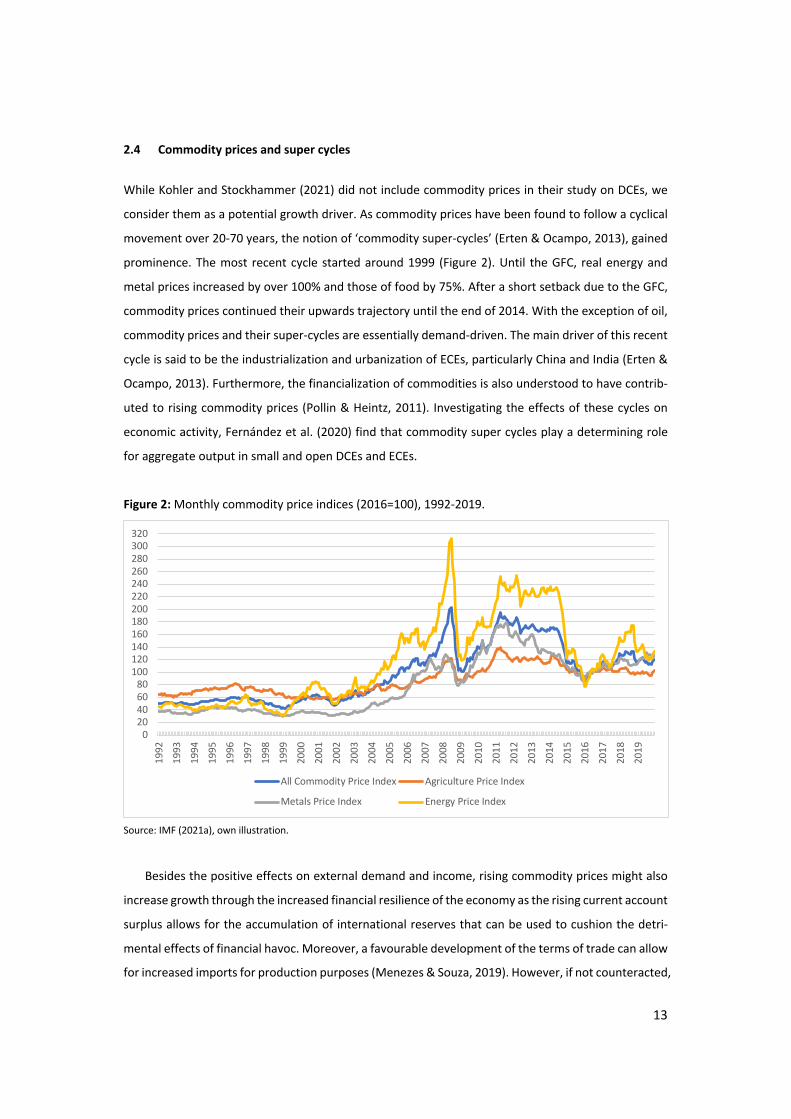
prominence. The most recent cycle started around 1999 (Figure 2). Until the GFC, real energy and

metal prices increased by over 100% and those of food by 75%. After a short setback due to the GFC,

commodity prices continued their upwards trajectory until the end of 2014. With the exception of oil,

commodity prices and their super-cycles are essentially demand-driven. The main driver of this recent

cycle is said to be the industrialization and urbanization of ECEs, particularly China and India (Erten &

Ocampo, 2013). Furthermore, the financialization of commodities is also understood to have contrib-

uted to rising commodity prices (Pollin & Heintz, 2011). Investigating the effects of these cycles on

economic activity, Fernández et al. (2020) find that commodity super cycles play a determining role

for aggregate output in small and open DCEs and ECEs.

Figure 2: Monthly commodity price indices (2016=100), 1992-2019.

Source: IMF (2021a), own illustration.

Besides the positive effects on external demand and income, rising commodity prices might also

increase growth through the increased financial resilience of the economy as the rising current account

surplus allows for the accumulation of international reserves that can be used to cushion the detri-

mental effects of financial havoc. Moreover, a favourable development of the terms of trade can allow

for increased imports for production purposes (Menezes & Souza, 2019). However, if not counteracted,

020406080

100120140160180200220240260280300320

19

92

19

93

19

94

19

95

19

96

19

97

19

98

19

99

20

00

20

01

20

02

20

03

20

04

20

05

20

06

20

07

20

08

20

09

20

10

20

11

20

12

20

13

20

14

20

15

20

16

20

17

20

18

20

19

All Commodity Price Index Agriculture Price Index

Metals Price Index Energy Price Index

14

the increased export volume can lead to real appreciation with detrimental effects on manufacturing

industries’ price competitiveness – as described by the concept of ‘Dutch disease’ (Bresser-Pereira,

2008). Evidently, possible positive effects of a secular rise in commodity prices can only occur in

commodity exporting countries while commodity import-dependent countries are likely to suffer. To

assess the cross-country effect of commodity prices, we will regress the countries’ growth on the

growth of a country-specific and weighted index of real commodity export prices.

2.5 Fiscal multipliers, hysteresis and autonomous demand-driven growth In recent years, a consensus on the positive effects of expansionary fiscal policy on macroeconomic

performance seems to have emerged (Stockhammer et al., 2019, pp. 58–60). This effect is commonly

associated with the notion of fiscal multipliers which refer to the increase in output induced by the

increase in public spending or decrease in taxation. Not only is there a large amount of literature that

finds fiscal multipliers to be larger than one, they also seem to be higher in recessions compared to

normal and upswing times as shown by the meta-regression analysis by Gechert and Rannenberg

(2018). This is commonly explained with fewer supply constraints and an accommodative monetary

policy stance during recessions. Additionally, fiscal multipliers of public spending are found to be larger

than those of taxation, while those of investment tend to exceed those of consumption. Furthermore,

multipliers are larger in more closed economies due to fewer demand leakages through imports

(Gechert & Rannenberg, 2018). For ECEs, several studies contend that fiscal multipliers are smaller

than for DCEs (Hory, 2016; Ilzetzki et al., 2013). Moreover, fiscal consolidation might have negative

hysteresis effects as the reductions in output might have long-term negative effects on the economic

performance while fiscal expansion could prevent such effects or even trigger positive ones (DeLong

& Summers, 2012; Gechert et al., 2019).

A more long-term perspective is taken in another strand of literature that introduces non-capacity

generating autonomous demand components into Kaleckian growth models. Allain (2015) uses auton-

omous government expenditure growth as such a demand component in a basic Kaleckian framework

with Harrodian instability. In the medium (and under certain conditions, long) run, it is the growth rate

of the autonomous demand component towards which the rate of accumulation converges. Therefore,

in this framework, higher growth rates of government expenditure imply higher rates of growth and

accumulation. While Allain avoids the treatment of government debt, Hein (2018) and Hein and Wood-

gate (2021) show that constant growth rates of government expenditure are under certain conditions

compatible with stable public debt to GDP ratios.

In their study, Kohler and Stockhammer (2021) find that expansionary fiscal policy drove post-GFC

growth in DCEs. To assess this relation for our sample, we will regress the general government balance

15

as an indicator of the fiscal policy stance on growth.7 In this respect, we deviate from the methodology

of Kohler and Stockhammer (2021) where the cyclically-adjusted fiscal balance to potential output was

employed to that end. We maintain that the demand-stabilising effect of fiscal policy also encompasses

its cyclical elements captured by the government balance. Moreover, the estimation of the output gap

that is needed to derive the cyclically-adjusted fiscal balance comes with several caveats (see e.g.

Heimberger & Kapeller, 2017). One downside, however, of using the general government balance is

that it does not necessarily indicate any intention of the identified fiscal policy stance. This concern is

addressed within a macroeconomic policy regime approach as recently conducted by Hein and

Martschin (2021), which is beyond the scope of the current paper.

3 Growth performance and drivers in 19 ECEs before and after the Global Financial Crisis

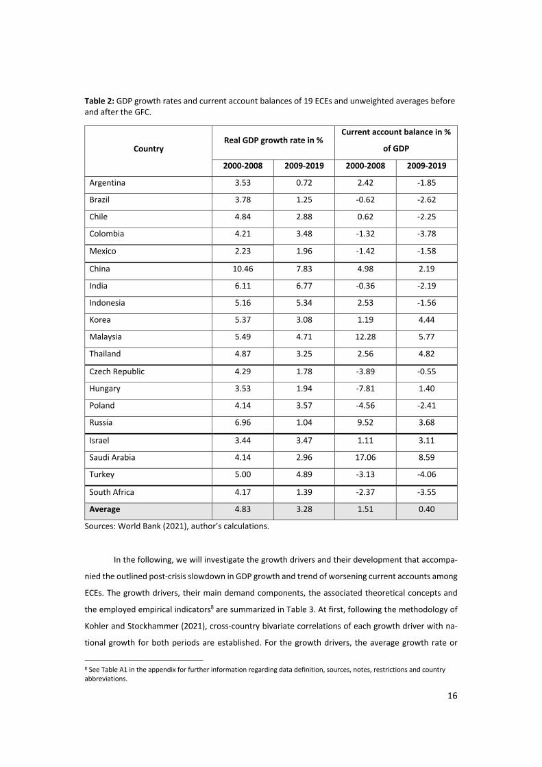
Table 2 depicts the average real GDP growth rates and current account balances of 19 ECEs in both

periods 2000-2008 and 2009-2019. After the GFC, ECEs grew less (3.28%) than before (4.83%). The

Chinese growth performance of 10.46% before and 7.83% after the GFC stands out while India and

Indonesia are the only ones that achieved higher growth rates after the crisis. Remarkable is the poor

performance within the Latin American countries, with Argentina and Brazil almost stagnating after

the GFC. Among the Central and Eastern European (CEE) countries, Poland’s post-crisis performance

stands out, especially when compared to Russia. Among the Middle Eastern countries, Turkey grew

slightly less after the GFC and Israel’s growth was roughly equal in both periods, whereas Saudi Arabia’s

growth fell considerably, as did that of South Africa. Although the development in terms of the current

account is more diverse, there is a trend of worsening current accounts after the crisis. While this

development was observable throughout the Latin American region, the current account improved on

average in Korea, Thailand, the Czech Republic, Hungary, Poland and Israel.

7 According to the literature on autonomous demand-driven growth, it would make sense to look at the growth of govern-

ment expenditure. However, government expenditure itself is a component of GDP and thus at odds with the definition of a

growth driver provided above.

16

Table 2: GDP growth rates and current account balances of 19 ECEs and unweighted averages before and after the GFC.

Country Real GDP growth rate in %

Current account balance in %

of GDP

2000-2008 2009-2019 2000-2008 2009-2019

Argentina 3.53 0.72 2.42 -1.85

Brazil 3.78 1.25 -0.62 -2.62

Chile 4.84 2.88 0.62 -2.25

Colombia 4.21 3.48 -1.32 -3.78

Mexico 2.23 1.96 -1.42 -1.58

China 10.46 7.83 4.98 2.19

India 6.11 6.77 -0.36 -2.19

Indonesia 5.16 5.34 2.53 -1.56

Korea 5.37 3.08 1.19 4.44

Malaysia 5.49 4.71 12.28 5.77

Thailand 4.87 3.25 2.56 4.82

Czech Republic 4.29 1.78 -3.89 -0.55

Hungary 3.53 1.94 -7.81 1.40

Poland 4.14 3.57 -4.56 -2.41

Russia 6.96 1.04 9.52 3.68

Israel 3.44 3.47 1.11 3.11

Saudi Arabia 4.14 2.96 17.06 8.59

Turkey 5.00 4.89 -3.13 -4.06

South Africa 4.17 1.39 -2.37 -3.55

Average 4.83 3.28 1.51 0.40

Sources: World Bank (2021), author’s calculations.

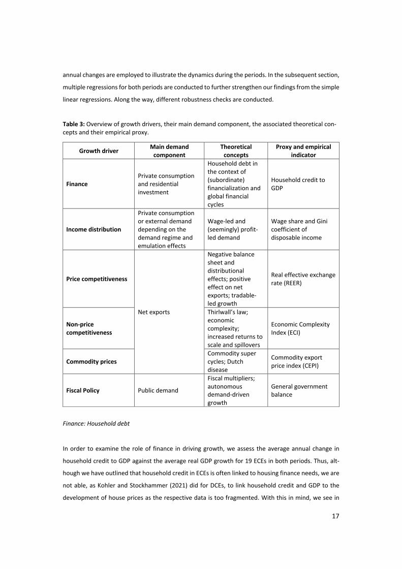
In the following, we will investigate the growth drivers and their development that accompa-

nied the outlined post-crisis slowdown in GDP growth and trend of worsening current accounts among

ECEs. The growth drivers, their main demand components, the associated theoretical concepts and

the employed empirical indicators8 are summarized in Table 3. At first, following the methodology of

Kohler and Stockhammer (2021), cross-country bivariate correlations of each growth driver with na-

tional growth for both periods are established. For the growth drivers, the average growth rate or

8 See Table A1 in the appendix for further information regarding data definition, sources, notes, restrictions and country

abbreviations.

17

annual changes are employed to illustrate the dynamics during the periods. In the subsequent section,

multiple regressions for both periods are conducted to further strengthen our findings from the simple

linear regressions. Along the way, different robustness checks are conducted.

Table 3: Overview of growth drivers, their main demand component, the associated theoretical con-cepts and their empirical proxy.

Growth driver Main demand

component Theoretical

concepts Proxy and empirical

indicator

Finance Private consumption and residential investment

Household debt in the context of (subordinate) financialization and global financial cycles

Household credit to GDP

Income distribution

Private consumption or external demand depending on the demand regime and emulation effects

Wage-led and (seemingly) profit-led demand

Wage share and Gini coefficient of disposable income

Price competitiveness

Net exports

Negative balance sheet and distributional effects; positive effect on net exports; tradable-led growth

Real effective exchange rate (REER)

Non-price competitiveness

Thirlwall’s law; economic complexity; increased returns to scale and spillovers

Economic Complexity Index (ECI)

Commodity prices Commodity super cycles; Dutch disease

Commodity export price index (CEPI)

Fiscal Policy Public demand

Fiscal multipliers; autonomous demand-driven growth

General government balance

Finance: Household debt

In order to examine the role of finance in driving growth, we assess the average annual change in

household credit to GDP against the average real GDP growth for 19 ECEs in both periods. Thus, alt-

hough we have outlined that household credit in ECEs is often linked to housing finance needs, we are

not able, as Kohler and Stockhammer (2021) did for DCEs, to link household credit and GDP to the

development of house prices as the respective data is too fragmented. With this in mind, we see in

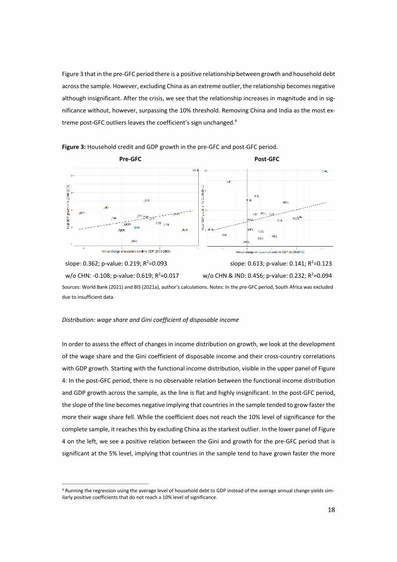
18

Figure 3 that in the pre-GFC period there is a positive relationship between growth and household debt

across the sample. However, excluding China as an extreme outlier, the relationship becomes negative

although insignificant. After the crisis, we see that the relationship increases in magnitude and in sig-

nificance without, however, surpassing the 10% threshold. Removing China and India as the most ex-

treme post-GFC outliers leaves the coefficient’s sign unchanged.9

Figure 3: Household credit and GDP growth in the pre-GFC and post-GFC period.

Pre-GFC Post-GFC

slope: 0.362; p-value: 0.219; R2=0.093 slope: 0.613; p-value: 0.141; R2=0.123

w/o CHN: -0.108; p-value: 0.619; R2=0.017 w/o CHN & IND: 0.456; p-value: 0.232; R2=0.094

Sources: World Bank (2021) and BIS (2021a), author’s calculations. Notes: In the pre-GFC period, South Africa was excluded

due to insufficient data.

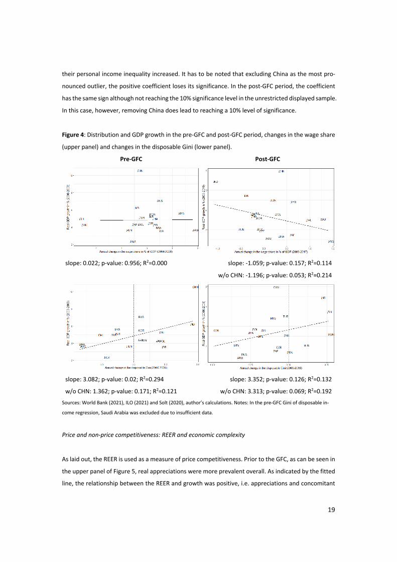
Distribution: wage share and Gini coefficient of disposable income

In order to assess the effect of changes in income distribution on growth, we look at the development

of the wage share and the Gini coefficient of disposable income and their cross-country correlations

with GDP growth. Starting with the functional income distribution, visible in the upper panel of Figure

4: In the post-GFC period, there is no observable relation between the functional income distribution

and GDP growth across the sample, as the line is flat and highly insignificant. In the post-GFC period,

the slope of the line becomes negative implying that countries in the sample tended to grow faster the

more their wage share fell. While the coefficient does not reach the 10% level of significance for the

complete sample, it reaches this by excluding China as the starkest outlier. In the lower panel of Figure

4 on the left, we see a positive relation between the Gini and growth for the pre-GFC period that is

significant at the 5% level, implying that countries in the sample tend to have grown faster the more

9 Running the regression using the average level of household debt to GDP instead of the average annual change yields sim-

ilarly positive coefficients that do not reach a 10% level of significance.

19

their personal income inequality increased. It has to be noted that excluding China as the most pro-

nounced outlier, the positive coefficient loses its significance. In the post-GFC period, the coefficient

has the same sign although not reaching the 10% significance level in the unrestricted displayed sample.

In this case, however, removing China does lead to reaching a 10% level of significance.

Figure 4: Distribution and GDP growth in the pre-GFC and post-GFC period, changes in the wage share

(upper panel) and changes in the disposable Gini (lower panel).

Pre-GFC Post-GFC

slope: 0.022; p-value: 0.956; R2=0.000 slope: -1.059; p-value: 0.157; R2=0.114

w/o CHN: -1.196; p-value: 0.053; R2=0.214

slope: 3.082; p-value: 0.02; R2=0.294

w/o CHN: 1.362; p-value: 0.171; R2=0.121

slope: 3.352; p-value: 0.126; R2=0.132

w/o CHN: 3.313; p-value: 0.069; R2=0.192

Sources: World Bank (2021), ILO (2021) and Solt (2020), author’s calculations. Notes: In the pre-GFC Gini of disposable in-

come regression, Saudi Arabia was excluded due to insufficient data.

Price and non-price competitiveness: REER and economic complexity

As laid out, the REER is used as a measure of price competitiveness. Prior to the GFC, as can be seen in

the upper panel of Figure 5, real appreciations were more prevalent overall. As indicated by the fitted

line, the relationship between the REER and growth was positive, i.e. appreciations and concomitant

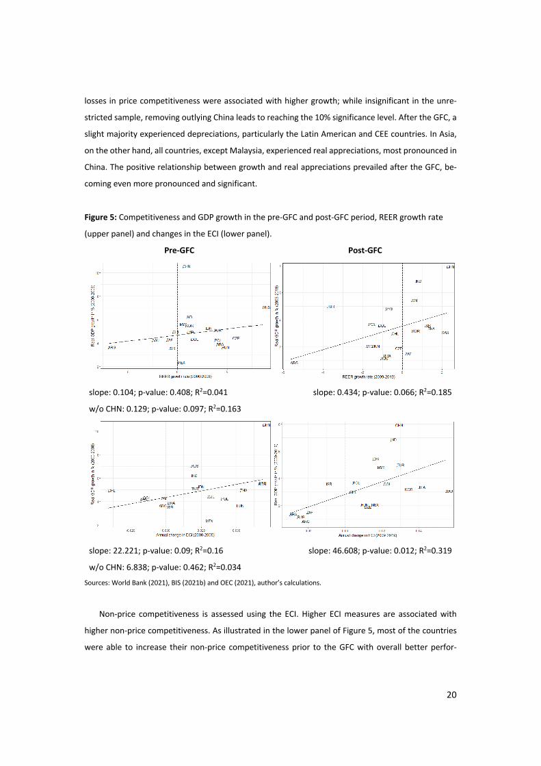
20

losses in price competitiveness were associated with higher growth; while insignificant in the unre-

stricted sample, removing outlying China leads to reaching the 10% significance level. After the GFC, a

slight majority experienced depreciations, particularly the Latin American and CEE countries. In Asia,

on the other hand, all countries, except Malaysia, experienced real appreciations, most pronounced in

China. The positive relationship between growth and real appreciations prevailed after the GFC, be-

coming even more pronounced and significant.

Figure 5: Competitiveness and GDP growth in the pre-GFC and post-GFC period, REER growth rate

(upper panel) and changes in the ECI (lower panel).

Pre-GFC Post-GFC

slope: 0.104; p-value: 0.408; R2=0.041

w/o CHN: 0.129; p-value: 0.097; R2=0.163

slope: 0.434; p-value: 0.066; R2=0.185

slope: 22.221; p-value: 0.09; R2=0.16

w/o CHN: 6.838; p-value: 0.462; R2=0.034

slope: 46.608; p-value: 0.012; R2=0.319

Sources: World Bank (2021), BIS (2021b) and OEC (2021), author’s calculations.

Non-price competitiveness is assessed using the ECI. Higher ECI measures are associated with

higher non-price competitiveness. As illustrated in the lower panel of Figure 5, most of the countries

were able to increase their non-price competitiveness prior to the GFC with overall better perfor-

21

mances among the CEE and Asian countries and poorer performances of South Africa, the Middle East-

ern and Latin American countries. Across the sample, we observe a positive relationship between non-

price competitiveness and growth. The slope coefficient is significant at the 10% level, thus suggesting

that non-price competitiveness drove growth during this period. However, the significance of the co-

efficient disappears when China as an outlier is removed. In the post-GFC period, the coefficient be-

comes even more pronounced and statistically significant.10

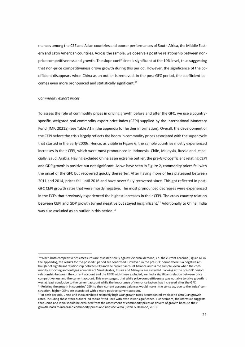
Commodity export prices

To assess the role of commodity prices in driving growth before and after the GFC, we use a country-

specific, weighted real commodity export price index (CEPI) supplied by the International Monetary

Fund (IMF, 2021a) (see Table A1 in the appendix for further information). Overall, the development of

the CEPI before the crisis largely reflects the boom in commodity prices associated with the super cycle

that started in the early 2000s. Hence, as visible in Figure 6, the sample countries mostly experienced

increases in their CEPI, which were most pronounced in Indonesia, Chile, Malaysia, Russia and, espe-

cially, Saudi Arabia. Having excluded China as an extreme outlier, the pre-GFC coefficient relating CEPI

and GDP growth is positive but not significant. As we have seen in Figure 2, commodity prices fell with

the onset of the GFC but recovered quickly thereafter. After having more or less plateaued between

2011 and 2014, prices fell until 2016 and have never fully recovered since. This got reflected in post-

GFC CEPI growth rates that were mostly negative. The most pronounced decreases were experienced

in the ECEs that previously experienced the highest increases in their CEPI. The cross-country relation

between CEPI and GDP growth turned negative but stayed insignificant.11 Additionally to China, India

was also excluded as an outlier in this period.12

10 When both competitiveness measures are assessed solely against external demand, i.e. the current account (Figure A1 in

the appendix), the results for the post-GFC period are confirmed. However, in the pre-GFC period there is a negative alt-

hough not significant relationship between ECI and the current account balance across the sample, even when the com-

modity exporting and outlying countries of Saudi Arabia, Russia and Malaysia are excluded. Looking at the pre-GFC period

relationship between the current account and the REER with those excluded, we find a significant relation between price

competitiveness and the current account. This may suggest that while price-competitiveness was not able to drive growth it

was at least conducive to the current account while the importance of non-price factors has increased after the GFC. 11 Relating the growth in countries’ CEPI to their current account balances would make little sense as, due to the index’ con-

struction, higher CEPIs are associated with a more positive current account. 12 In both periods, China and India exhibited relatively high GDP growth rates accompanied by close to zero CEPI growth

rates. Including these stark outliers led to flat fitted lines with even lower significance. Furthermore, the literature suggests

that China and India should be excluded from the assessment of commodity prices as drivers of growth because their

growth leads to increased commodity prices and not vice versa (Erten & Ocampo, 2013).

22

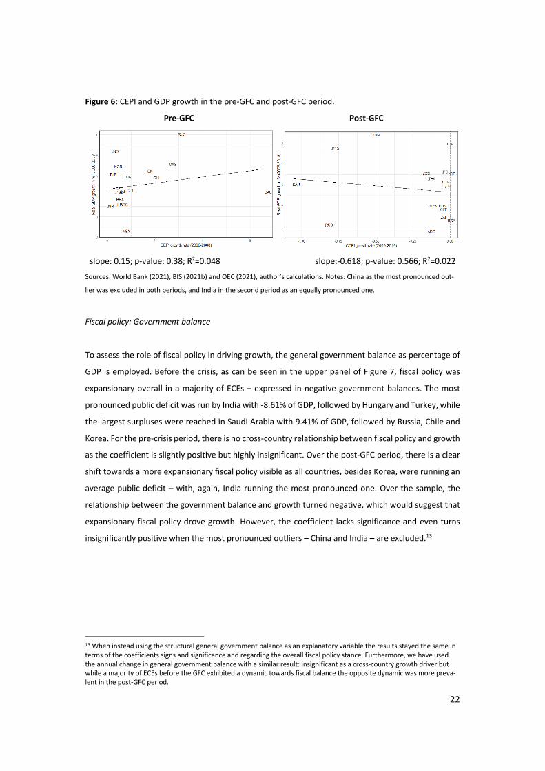
Figure 6: CEPI and GDP growth in the pre-GFC and post-GFC period.

Pre-GFC Post-GFC

slope: 0.15; p-value: 0.38; R2=0.048 slope:-0.618; p-value: 0.566; R2=0.022

Sources: World Bank (2021), BIS (2021b) and OEC (2021), author’s calculations. Notes: China as the most pronounced out-

lier was excluded in both periods, and India in the second period as an equally pronounced one.

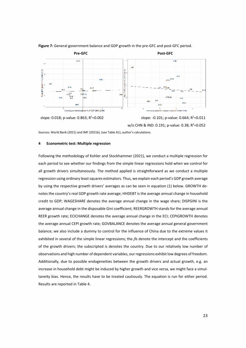
Fiscal policy: Government balance

To assess the role of fiscal policy in driving growth, the general government balance as percentage of

GDP is employed. Before the crisis, as can be seen in the upper panel of Figure 7, fiscal policy was

expansionary overall in a majority of ECEs – expressed in negative government balances. The most

pronounced public deficit was run by India with -8.61% of GDP, followed by Hungary and Turkey, while

the largest surpluses were reached in Saudi Arabia with 9.41% of GDP, followed by Russia, Chile and

Korea. For the pre-crisis period, there is no cross-country relationship between fiscal policy and growth

as the coefficient is slightly positive but highly insignificant. Over the post-GFC period, there is a clear

shift towards a more expansionary fiscal policy visible as all countries, besides Korea, were running an

average public deficit – with, again, India running the most pronounced one. Over the sample, the

relationship between the government balance and growth turned negative, which would suggest that

expansionary fiscal policy drove growth. However, the coefficient lacks significance and even turns

insignificantly positive when the most pronounced outliers – China and India – are excluded.13

13 When instead using the structural general government balance as an explanatory variable the results stayed the same in

terms of the coefficients signs and significance and regarding the overall fiscal policy stance. Furthermore, we have used

the annual change in general government balance with a similar result: insignificant as a cross-country growth driver but

while a majority of ECEs before the GFC exhibited a dynamic towards fiscal balance the opposite dynamic was more preva-

lent in the post-GFC period.

23

Figure 7: General government balance and GDP growth in the pre-GFC and post-GFC period.

Pre-GFC Post-GFC


w/o CHN & IND: 0.191; p-value: 0.38; R2=0.052

Sources: World Bank (2021) and IMF (2021b), (see Table A1), author’s calculations.

4 Econometric test: Multiple regression

Following the methodology of Kohler and Stockhammer (2021), we conduct a multiple regression for

each period to see whether our findings from the simple linear regressions hold when we control for

all growth drivers simultaneously. The method applied is straightforward as we conduct a multiple

regression using ordinary least squares estimators. Thus, we explain each period’s GDP growth average

by using the respective growth drivers’ averages as can be seen in equation (1) below. GROWTH de-

notes the country’s real GDP growth rate average; HHDEBT is the average annual change in household

credit to GDP; WAGESHARE denotes the average annual change in the wage share; DISPGINI is the

average annual change in the disposable Gini coefficient; REERGROWTH stands for the average annual

REER growth rate; ECICHANGE denotes the average annual change in the ECI; CEPIGROWTH denotes

the average annual CEPI growth rate; GOVBALANCE denotes the average annual general government

balance; we also include a dummy to control for the influence of China due to the extreme values it

exhibited in several of the simple linear regressions; the bs denote the intercept and the coefficients

of the growth drivers; the subscripted is denotes the country. Due to our relatively low number of

observations and high number of dependent variables, our regressions exhibit low degrees of freedom.

Additionally, due to possible endogeneities between the growth drivers and actual growth, e.g. an

increase in household debt might be induced by higher growth and vice versa, we might face a simul-

taneity bias. Hence, the results have to be treated cautiously. The equation is run for either period.

Results are reported in Table 4.

24

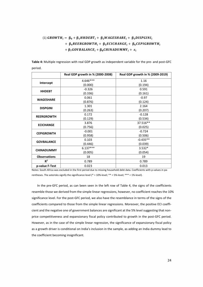
(1) !"#$%&! =)" + )#&&+,-%! +)$$.!,/&.",! +)%+0/1!020!+)&",,"!"#$%&! +)',303&.2!,! +)(3,10!"#$%&!

+ ))!#4-.5.23,! + )*3&02.+6778! +9!

Table 4: Multiple regression with real GDP growth as independent variable for the pre- and post-GFC

period.

Real GDP growth in % (2000-2008) Real GDP growth in % (2009-2019)

Intercept 4.646*** (0.000)

1.16 (0.194)

HHDEBT -0.326 (0.336)

0.591 (0.161)

WAGESHARE 0.061

(0.876) -0.97

(0.124)

DISPGINI 1.301

(0.263) 2.164

(0.207)

REERGROWTH 0.172

(0.129) -0.128 (0.534)

ECICHANGE 3.876

(0.756) 37.516** (0.025)

CEPIGROWTH -0.001 (0.958)

-0.724 (0.506)

GOVBALANCE 0.103

(0.446) -0.435** (0.039)

CHINADUMMY 6.137*** (0.005)

3.532* (0.054)

Observations 18 19 R2 0.789 0.789

p-value F-Test 0.023 0.013 Notes: South Africa was excluded in the first period due to missing household debt data. Coefficients with p-values in pa-

rentheses. The asterisks signify the significance level (* = 10%-level; ** = 5%-level; *** = 1%-level).

In the pre-GFC period, as can been seen in the left row of Table 4, the signs of the coefficients

resemble those we derived from the simple linear regressions, however, no coefficient reaches the 10%

significance level. For the post-GFC period, we also have the resemblance in terms of the signs of the

coefficients compared to those from the simple linear regressions. Moreover, the positive ECI coeffi-

cient and the negative one of government balances are significant at the 5% level suggesting that non-

price competitiveness and expansionary fiscal policy contributed to growth in the post-GFC period.

However, as in the case of the simple linear regression, the significance of expansionary fiscal policy

as a growth driver is conditional on India’s inclusion in the sample, as adding an India dummy lead to

the coefficient becoming insignificant.

25

5 Discussion: Heterogeneity amidst entrenched financialization and expansionary fiscal policy

Before further assessing our results, some caveats regarding the methodology should be recalled. First,

we do establish coefficients that, at best, signify a correlation between the respective variables. As is

known, correlations are not causalities, however, for causalities to exist there have to be correlations.

Furthermore, it must be emphasized that the coefficients we derive are cross-country ones. Thus, fail-

ing to establish a cross-country correlation does not mean that this indicator was not relevant for every

country but might be a sign of heterogeneity within the sample. Moreover, certain empirical indicators

were only available in a restricted sense that could shape the results (see Table A1). Finally, the GFC is

not the only structural breaking point one could think of. Besides the possibility of countries exhibiting

heterogeneity in their structural breaking points as well, we will elaborate on two potentially alterna-

tive breaking points: the ‘taper tantrum’ in 2013 and the fall in commodity prices after 2014.

These caveats in mind, we have seen that ECEs overall grew slower after the GFC than they did

before with a trend towards worsening current account balances (Table 2). In terms of cross-country

growth drivers, significant and robust results are sparse. The simple and multiple linear regressions

suggest to some extent that household debt has become more important in the post-GFC period in

driving growth although with lacking significance when we control for China (Figure 3, Table 4).14

Meanwhile, it is evident that the post-GFC period was overall marked by further entrenched financial-

ization in terms of household debt as only Hungary, South Africa and India experienced private delev-

eraging over the period. Failing to observe the cross-country importance of financial factors in driving

growth of ECEs – as in the case of DCEs (Kohler & Stockhammer, 2021) – against the background of

progressing financialization, points at several issues: First, this hints at the heterogeneity among the

investigated ECEs in terms of their ‘variegated’ forms of financialization (Karwowski, 2020) and GMs

(Akcay et al., 2021). Thus, ECEs’ growth materializes through distinct demand components that rely on

diverse growth drivers with household debt only playing a major role in some constellations. Further-

more, the subordinate nature of ECEs’ financialization weakens the relation between their financial

factors and domestic economic conditions. Instead, capital inflows and credit growth in financially

open ECEs correlate with developments in DCEs, like loose US monetary policy (Bonizzi, 2017b; Bräun-

ing & Ivashina, 2020). A recent and prominent example of this phenomenon was the ‘taper tantrum’

of 2013 when ECEs faced sustained capital outflows following the US Federal Reserve’s announcement

of future monetary policy tightening (Akyüz, 2021). Figure 8 visualizes this: household debt in ECEs

14 As noted earlier, we have used household credit instead of private credit as a whole due to the financialization tenden-

cies among ECEs’ NFCs, which lead to increasing usage of debt for financial instead of real purposes. However, in countries

such as Turkey (Orhangazi & Yeldan, 2021) or China (Chen & Kang, 2018) NFC debt fuels activity in non-tradable sectors and

is thus a possible growth driver. However, performing the regressions with total private credit or NFC credit leads to the

same results in terms of signs and significance as with household credit.

26

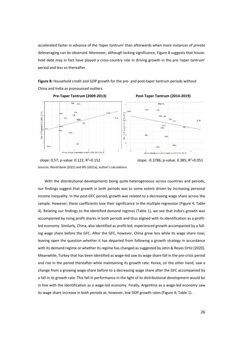
accelerated faster in advance of the ‘taper tantrum’ than afterwards when more instances of private

deleveraging can be observed. Moreover, although lacking significance, Figure 8 suggests that house-

hold debt may in fact have played a cross-country role in driving growth in the pre-‘taper tantrum’

period and less so thereafter.

Figure 8: Household credit and GDP growth for the pre- and post-taper tantrum periods without

China and India as pronounced outliers.

Pre-Taper Tantrum (2009-2013) Post-Taper Tantrum (2014-2019)


Sources: World Bank (2021) and BIS (2021a), author’s calculations.

With the distributional developments being quite heterogeneous across countries and periods,

our findings suggest that growth in both periods was to some extent driven by increasing personal

income inequality. In the post-GFC period, growth was related to a decreasing wage share across the

sample. However, these coefficients lose their significance in the multiple regression (Figure 4; Table

4). Relating our findings to the identified demand regimes (Table 1), we see that India’s growth was

accompanied by rising profit shares in both periods and thus aligned with its identification as a profit-

led economy. Similarly, China, also identified as profit-led, experienced growth accompanied by a fall-

ing wage share before the GFC. After the GFC, however, China grew less while its wage share rose;

leaving open the question whether it has departed from following a growth strategy in accordance

with its demand regime or whether its regime has changed as suggested by Jetin & Reyes Ortiz (2020).

Meanwhile, Turkey that has been identified as wage-led saw its wage share fall in the pre-crisis period

and rise in the period thereafter while maintaining its growth rate. Korea, on the other hand, saw a

change from a growing wage-share before to a decreasing wage share after the GFC accompanied by

a fall in its growth rate. This fall in performance in the light of its distributional development would be

in line with the identification as a wage-led economy. Finally, Argentina as a wage-led economy saw

its wage share increase in both periods at, however, low GDP growth rates (Figure 4; Table 1).

27

As we have pointed out, distribution as a growth driver is connected to price competitiveness.

Despite some indications of cross-country profit-led growth following the GFC, we have found no indi-

cation for a cross-country relation between growth and price competitiveness in both periods (Figure

5; Table 4) – similarly to Kohler and Stockhammer (2021) for DCEs. Besides the mentioned reasons of

heterogeneity, the absence of price competitiveness as a growth driver may be due to the negative

balance sheet effects associated with real depreciations (Krugman, 1999), especially, in the light of

progressed financialization which in ECEs comes also with increased foreign currency denominated

debt (e.g. McCauley et al., 2015). Moreover, import dependencies may narrow the possible gains from

depreciations. But furthermore, the lack of price competitiveness as a growth driver raises the ques-

tion how rising income inequality and profit shares translated into growth in our sample as the com-

mon mechanism through which such redistribution fosters growth is via increased price competitive-

ness boosting net exports. Theoretically, higher profit shares can foster growth via inducing investment

due to increased profitability. But significant empirical support for this mechanism is rare (Hein, 2014,

p. 300). Alternatively, the positive relation between rising inequality and higher GDP growth might be

a manifestation of seemingly profit-led demand (Hein & Prante, 2020). At least for the post-GFC period,

the tightened connection between household credit and growth would suggest this relation of rising

household indebtedness in the face of rising income inequality is one mechanism that may give rise to

seemingly profit-led demand (see Kapeller & Schütz, 2015). But running regressions to assess the rela-

tion between rising profit shares and income inequality, on the one hand, and household debt on the

other do not indicate such relation (see Figure A2 in the appendix).

While questions remain open in the realm of distribution, our results in terms of non-price com-

petitiveness are more straightforward as they suggest that non-price factors drove growth, particularly

in the post-GFC period. These findings are in line with the literature on economic complexity (Hidalgo

& Hausmann, 2009), Thirlwall's (1979) law, and economic structuralism (e.g. Ocampo & Parra, 2006).

Furthermore, in terms of the importance of non-price competitiveness, ECEs resemble DCEs (Gräbner

et al., 2020; Hein and Martschin, 2021; Kohler & Stockhammer, 2021). In both periods, the most pro-

nounced increases in that regard were made by the Asian countries while the Middle Eastern and CEE

countries were less consistent and the Latin American countries performed poorly overall (Figure 5;

Table 4). Conversely, our results do not contain a significant cross-country relation between GDP and

commodity prices. One reason for this absence besides ECEs’ heterogeneity, might be the periodiza-

tion with the GFC as the breaking point. However, assessing the relation in accordance with the super

cycle, i.e. choosing 2000-2014, did not alter the results (see Figure A3 in the appendix). Meanwhile,

fiscal policy became more expansionary after the GFC across the sample; however, robust and signifi-

cant findings for it driving growth are conditional on India’s presence in the sample, given that it grew

at relatively high rates accompanied by a pronounced fiscal deficit (Figure 7; Table 4).

28

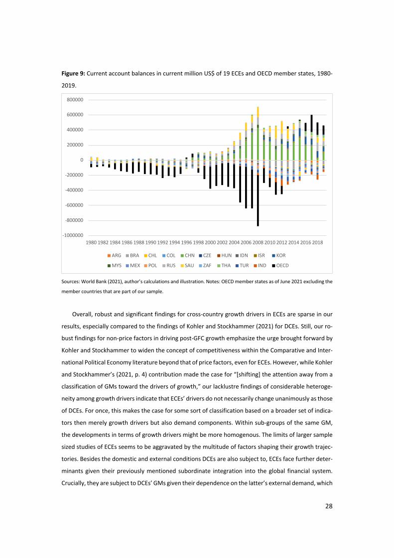
Figure 9: Current account balances in current million US$ of 19 ECEs and OECD member states, 1980-

2019.

Sources: World Bank (2021), author’s calculations and illustration. Notes: OECD member states as of June 2021 excluding the

member countries that are part of our sample.

Overall, robust and significant findings for cross-country growth drivers in ECEs are sparse in our

results, especially compared to the findings of Kohler and Stockhammer (2021) for DCEs. Still, our ro-

bust findings for non-price factors in driving post-GFC growth emphasize the urge brought forward by

Kohler and Stockhammer to widen the concept of competitiveness within the Comparative and Inter-

national Political Economy literature beyond that of price factors, even for ECEs. However, while Kohler

and Stockhammer’s (2021, p. 4) contribution made the case for “[shifting] the attention away from a

classification of GMs toward the drivers of growth,” our lacklustre findings of considerable heteroge-

neity among growth drivers indicate that ECEs’ drivers do not necessarily change unanimously as those

of DCEs. For once, this makes the case for some sort of classification based on a broader set of indica-

tors then merely growth drivers but also demand components. Within sub-groups of the same GM,

the developments in terms of growth drivers might be more homogenous. The limits of larger sample

sized studies of ECEs seems to be aggravated by the multitude of factors shaping their growth trajec-

tories. Besides the domestic and external conditions DCEs are also subject to, ECEs face further deter-

minants given their previously mentioned subordinate integration into the global financial system.

Crucially, they are subject to DCEs’ GMs given their dependence on the latter’s external demand, which

-1000000

-800000

-600000

-400000

-200000

0

200000

400000

600000

800000

1980 1982 1984 1986 1988 1990 1992 1994 1996 1998 2000 2002 2004 2006 2008 2010 2012 2014 2016 2018

ARG BRA CHL COL CHN CZE HUN IDN ISR KOR

MYS MEX POL RUS SAU ZAF THA TUR IND OECD

29

thus determines the feasibility of export-led GMs in ECEs. In that sense, an increase in the importance

of household debt in driving ECEs post-GFC growth – for which we have seen some indications – would

be expected as a form of demand compensation following the increased export-led GMs among ECEs

(Hein et al., 2021) and their reduced imports, respectively (Kohler & Stockhammer, 2021). This is ex-

pressed in the worsened current accounts of ECEs vis-à-vis DCEs as visualized by Figure 9: Prior to the

GFC, several ECEs ran current account surpluses matched by deficits in the DCEs. After the GFC, public

demand in DCEs only insufficiently substituted the private demand drag in DCEs caused by private

deleveraging. Figure 9 visualizes this with the aggregation of the current accounts of the OECD coun-

tries, excluding those that are part of our sample. Not only did the aggregated current account deficit

of DCEs shrink after the GFC, it became roughly balanced since 2013 and turned into a surplus in 2016.

6 Conclusions We have seen that ECEs grew slower after the GFC with a trend towards worsening current account

balances. In terms of robust cross-country growth drivers, our results are sparse with the exception of

non-price competitiveness that drove growth, particularly, in the post-crisis period while there are no

indications of price competitiveness and commodity prices in driving growth across our sample. The

absence of price competitiveness as a cross-country growth driver is particularly remarkable against

some indications of growth being accompanied by increasing income inequality during both periods

and with falling wage shares in the post-crisis years. Against the overall further entrenchment of finan-

cialization in ECEs in terms of rising household debt, there are indications that growth has become

more dependent on rising household debt in the post-GFC period, especially in the years before 2014

when ECEs experienced pronounced capital inflows fuelled by the loose US monetary policy. Similarly,

fiscal policy turned more expansionary in these countries following the GFC but without becoming a

robust cross-country growth driver. We argue that the absence of robust cross-country growth drivers

among ECEs reflects their heterogeneity, for instance, in terms of their ‘variegated’ financialization

(Karwowski, 2020) and GMs (Akcay et al., 2021). Thus, in order to understand the post-crisis trajectory

of ECEs, the investigation of growth drivers should be completed by further clustering. This could be

done along the lines of different demand components’ growth contributions and sectoral financial

balances as in Akcay et al. (2021), financial factors (Karwowski, 2020; Fernandez & Aalbers, 2020), the

importance of commodity exports or their ‘type of capitalism’ (Schedelik et al. 2021). Moreover, fur-

ther research should investigate the economic policy in ECEs on this trajectory as in the macroeco-

nomic policy-regime approach (Hein & Martschin, 2021) to shed light on the issue what ultimately

determines ECEs’ GMs and what scope national strategies have in light of the multitude of dependen-

cies ECEs face.

30

References

Ahmed, S., & Zlate, A. (2014). Capital flows to emerging market economies: A brave new world? Jour-

nal of International Money and Finance, 48, Part B, 221–248. Akcay, Ü., Hein, E., & Jungmann, B. (2021). Financialisation and macroeconomic regimes in emerging

capitalist economies before and after the Great Recession. Institute for International Political

Economy (IPE) Berlin, Working Paper, 158. Retrieved 24 June 2021, from https://www.ipe-berlin.org/fileadmin/institut-ipe/Dokumente/Working_Papers/ipe_working_paper_158.pdf

Akkemik, K., & Özen, S. (2014). Macroeconomic and institutional determinants of financialization of non-financial firms: case study of Turkey. Socio-Economic Review, 12(1), 71–98.

Akyüz, Y. (2021). External balance sheets of emerging economies: Low-yielding assets, high-yielding liabilities. Review of Keynesian Economics, 9(2), 232–252.

Alarco, G. (2016). Distribución factorial del ingreso y regímenes de crecimiento en América Latina, 1950-2012. Revista Internacional del Trabajo, 135(1), 79–103.

Allain, O. (2015). Tackling the instability of growth: A Kaleckian-Harrodian model with an autono-mous expenditure component. Cambridge Journal of Economics, 39(5), 1351–1371.

Araújo, E., & Gala, P. (2012). Economic growth regimes in Brazil: Empirical evidence and policy impli-cations. Estudos Avançados, 26(75), 41–56.

Arestis, P., & Glickman, M. (2002). Financial crisis in Southeast Asia: Dispelling illusion the Minskyan way. Cambridge Journal of Economics, 26(2), 237–260.

Ashman, S., Fine, B., & Newman, S. (2011). The crisis in South Africa: Neoliberalism, financialization and uneven and combined development. Socialist Register, 47, 174-195.

Baccaro, L., & Pontusson, J. (2016). Rethinking comparative political economy: The growth model perspective. Politics & Society, 44(2), 175–207.

Bhaduri, A., & Marglin, S. (1990). Unemployment and the real wage: The economic basis for contest-ing political ideologies. Cambridge Journal of Economics, 14(4), 375–393.

Bird, M. (2020). Chinese household debt surges through the pandemic. Retrieved 20 July 2021, from The Wall Street Journal website: https://www.wsj.com/articles/chinese-household-debt-surges-through-the-pandemic-11607417329

Bonizzi, B. (2017a). An alternative Post-Keynesian framework for understanding capital flows to emerging markets. Journal of Economic Issues, 51(1), 137-162.

Bonizzi, B. (2017b). International financialisation, developing countries and the contradictions of pri-vatised Keynesianism. Economic and Political Studies, 5(1), 21–40.

Bortz, P. G., & Kaltenbrunner, A. (2018). The international dimension of financialization in developing and emerging economies. Development and Change, 49(2), 375–393.

Bräuning, F., & Ivashina, V. (2020). U.S. monetary policy and emerging market credit cycles. Journal

of Monetary Economics, 112, 57–76. Bresser-Pereira, L. C. (2008). The Dutch disease and its neutralization: A Ricardian approach. Brazilian

Journal of Political Economy, 28(1), 47–71. Chen, S., & Kang, J. S. (2018). Credit Booms – Is China different? IMF Working Paper 18/2.

https://doi.org/10.5089/9781484336762.001 Chang, K.-S. (2016). Financialization of poverty: Proletarianizing the Financial Crisis in post-develop-

mental Korea. In S. Soederberg (Ed.), Risking capitalism: Volume 31 (pp. 109-134). Bingley, UK: Emerald Publishing.

Charpe, M., Lee, S., Arias, D., & Bridji, S. (2014). Does income distribution matter for development? Trends in labour share of income and their economic impacts in developing countries. World

of Work Report, 2014(1), 149–180. Correa, E., Vidal, G., & Marshall W. (2012). Financialization in Mexico: Trajectory and Limits. Journal

of Post Keynesian Economics, 35(2), 255–275.

31

de Jesus, C. S., Araujo, R. A., & Drumond, C. E. (2018). An empirical test of the Post-Keynesian growth model applied to functional income distribution and the growth regime in Brazil. Interna-

tional Review of Applied Economics, 32(4), 428–449. DeLong, J. B., & Summers, L. H. (2012). Fiscal policy in a depressed economy. Brookings Papers on

Economic Activity, Spring 2012, 233–297. Demir, F. (2007). The rise of rentier capitalism and the financialization of real sectors in developing

countries. Review of Radical Political Economics, 39(3), 351–359. Demir, F. (2009). Financial liberalization, private investment and portfolio choice: Financialization of

real sectors in emerging markets. Journal of Development Economics, 88(2), 314–324. Dodig, N., Hein, E., & Detzer, D. (2016). Financialisation and the financial and economic crises: Theo-

retical framework and empirical analysis for 15 countries. In E. Hein, D. Detzer, & N. Dodig (eds.), Financialisation and the financial and economic crises (pp. 1–41). Cheltenham, UK: Ed-ward Elgar.

Dos Santos, P.L. (2013). A cause for policy concern: The expansion of household credit in middle-in-come economies. International Review of Applied Economics, 27(3), 316-338.

Epstein, G. A. (2005). Introduction. In Financialization and the world economy (pp. 5–21). Chelten-ham, UK: Edward Elgar.

Erten, B., & Ocampo, J. A. (2013). Super cycles of commodity prices since the mid-nineteenth cen-tury. World Development, 44, 14–30.

Farhi, M., & Borghi, R.A.Z. (2009). Operations with Financial Derivatives of Corporations from Emerg-ing Economies. Estudos Avançados, 23(66), 169–88.

Fernández, A., Schmitt-Grohé, S., & Uribe, M. (2020). Does the commodity super cycle matter? Na-

tional Bureau of Economic Research, Working Paper, 27589. Retrieved 24 June 2021, from https://www.nber.org/system/files/working_papers/w27589/w27589.pdf

Fernandez, R., & Aalbers, M. B. (2020). Housing financialization in the Global South: In search for a comparative framework. Housing Policy Debate, 30(4), 680-701.

Gabor, D. (2010). (De)Financialization and Crisis in Eastern Europe. Competition and Change, 14(3-4), 248–270.

Gala, P., Rocha, I., & Magacho, G. (2018). The structuralist revenge: Economic complexity as an im-portant dimension to evaluate growth and development. Brazilian Journal of Political Econ-

omy, 38(2), 219–236. Gechert, S., Horn, G., & Paetz, C. (2019). Long-term effects of fiscal stimulus and austerity in Europe.

Oxford Bulletin of Economics and Statistics, 81(3), 647–666. Gechert, S., & Rannenberg, A. (2018). Which fiscal multipliers are regime-dependent? A meta-regres-

sion analysis. Journal of Economic Surveys, 32(4), 1160–1182. Gouvêa, R. R., & Lima, G. T. (2010). Structural change, balance-of-payments constraint, and economic

growth: Evidence from the multisectoral Thirlwall’s law. Journal of Post Keynesian Economics, 33(1), 169–204.

Gräbner, C., Heimberger, P., Kapeller, J., & Schütz, B. (2020). Is the Eurozone disintegrating? Macroe-conomic divergence, structural polarisation, trade and fragility. Cambridge Journal of Eco-

nomics, 44(3), 647–669. Heimberger, P., & Kapeller, J. (2017). The performativity of potential output: Pro-cyclicality and path

dependency in coordinating European fiscal policies. Review of International Political Econ-

omy, 24(5), 904–928. Hall, P. A. (2018). Varieties of Capitalism in light of the euro crisis. Journal of European Public Policy,

25(1), 7-30. Hein, E. (2014). Distribution and growth after Keynes: A Post-Keynesian guide. Cheltenham, UK: Ed-

ward Elgar. Hein, E. (2018). Autonomous government expenditure growth, deficits, debt, and distribution in a

neo-Kaleckian growth model. Journal of Post Keynesian Economics, 41(2), 316–338. Hein, E., & Martschin, J. (2021). Demand and growth regimes in finance-dominated capitalism and

the role of the macroeconomic policy regime: a post-Keynesian comparative study on France,

32

Germany, Italy and Spain before and after the Great Financial Crisis and the Great Recession. Review of Evolutionary Political Economy, advance access, 1-35.

Hein, E., Meloni, W. P., & Tridico, P. (2021). Welfare models and demand-led growth regimes before and after the financial and economic crisis. Review of International Political Economy, 28(5), 1196–1223.

Hein, E., & Mundt, M. (2012). Financialisation and the requirements and potentials for wage-led re-

covery: A review focussing on the G20. Geneva: ILO. Hein, E., & Prante, F. J. (2020). Functional distribution and wage inequality in recent Kaleckian growth

models. In H. Bougrine, & L.-P., Rochon (eds.), Economic Growth and Macroeconomic Stabili-

zation Policies in Post-Keynesian Economics (pp. 33-49). Cheltenham, UK: Edward Elgar. Hein, E., & Woodgate, R. (2021). Stability issues in Kaleckian models driven by autonomous demand

growth – Harrodian instability and debt dynamics. Metroeconomica, 72(2), 388-404. Hidalgo, C. A., & Hausmann, R. (2009). The building blocks of economic complexity. Proceedings of

the National Academy of Sciences, 106(26), 10570–10575. Hory, M.-P. (2016). Fiscal multipliers in emerging market economies: Can we learn something from

advanced economies? International Economics, 146, 59–84. Ilzetzki, E., Mendoza, E. G., & Végh, C. A. (2013). How big (small?) are fiscal multipliers? Journal of

Monetary Economics, 60(2), 239–254. Isaacs, G., & Kaltenbrunner, A. (2018). Financialization and liberalization: South Africa’s new forms of

external vulnerability. Competition & Change, 22(4), 437–463. Jetin, B., & Kurt, O. E. (2016). Functional income distribution and growth in Thailand: A post Keynes-

ian econometric analysis. Journal of Post Keynesian Economics, 39(3), 334–360. Jetin, B., & Reyes Ortiz, L. (2020). Wage-led demand as a rebalancing strategy for economic growth in

China. Journal of Post Keynesian Economics, 43(3), 341–366. Jiménez, V. (2020). Wage shares and demand regimes in Central America: An empirical analysis 1970-

2016. Institute for International Political Economy (IPE) Berlin, Working Paper, 151. Retrieved 24 June 2021, from https://www.ipe-berlin.org/fileadmin/institut-ipe/Dokumente/Work-ing_Papers/ipe_working_paper_151.pdf

Johnston, A., & Regan, A. (2018). Introduction: Is the European Union capable of integrating diverse models of Capitalism? New Political Economy, 23(2), 145-159.

Joo, S., Lee, K., Nah, W. J., Jeon, S. M., & Joe, D. H. (2020). The income-led growth in Korea: Status, prospects and lessons for other countries. Korea Institute for International Economic Policy, Research Paper, Policy Analysis 20-01.

Kalinowski, T., & Cho, H. (2009). The Political Economy of Financial Liberalization in South Korea: State, Big Business, and Foreign Investors. Asian Survey, 49(2), 221–242.

Kaltenbrunner, A., & Painceira, J. P. (2015). Developing countries’ changing nature of financial inte-gration and new forms of external vulnerability: The Brazilian experience. Cambridge Journal

of Economics, 39(5), 1281–1306. Kaltenbrunner, A., & Painceira, J. P. (2018). Subordinated financial integration and financialisation in

emerging capitalist economies: The Brazilian experience. New Political Economy, 23(3), 290–313.

Kapeller, J., & B. Schütz (2015). Conspicuous consumption, inequality and debt: the nature of consumption driven profit-led regimes, Metroeconomica, 66(1), 51–70.

Karacimen, E. (2016). Consumer credit as an aspect of everyday life of workers in developing coun-tries: Evidence from Turkey. Review of Radical Political Economics, 48(2), 252-268.

Karwowski, E. (2012). Financial Operations of South African Listed Firms: Growth and Financial Stabil-ity in an Emerging Market Setting. Paper presented at iii conferencia international do ieSe, Maputo, Mozambique, 3-4 September. Retrieved 16 July 2021, from https://www.iese.ac.mz/~ieseacmz/lib/publication/III_Conf2012/IESE_IIIConf_Paper6.pdf

Karwowski, E. (2020). Economic development and variegated financialization in emerging economies. In P. Mader, D. Mertens, & N. van der Zwan (Eds.), The Routledge International Handbook of

Financialization (pp. 162–176). London: Routledge.

33

Karwowski, E., & Stockhammer, E. (2017). Financialisation in emerging economies: a systematic over-view and comparison with Anglo-Saxon economies. Economic and Political Studies, 5(1), 60-86.

Kohler, K., & Stockhammer, E. (2021). Growing differently? Financial cycles, austerity, and competi-tiveness in growth models since the Global Financial Crisis. Review of International Political

Economy, advance access, 1–28. Kohli, V. (2018). Functional income distribution and effective demand in India: An applied post

Keynesian model. Journal of Post Keynesian Economics, 41(3), 399–429. Krugman, P. (1999). Balance sheets, the transfer problem, and financial crises. International Tax and

Public Finance, 6, 459–472. Kurt, O. E. (2018). Functional income distribution and growth in South Korea: A Post Keynesian Econ-

ometric Analysis. Marmara Üniversitesi İktisadi ve İdari Bilimler Dergisi, 39(2), 553–576. Lavoie, M. (2009). Cadrisme within a Kaleckian model of growth and distribution, Review of Political

Economy, 21(3), 371–393. Lavoie, M., & Stockhammer, E. (2013). Wage-led growth: concept, theories and policies. In M. Lavoie,

& E. Stockhammer (eds.), Wage-led growth: An equitable strategy for economic recovery (pp. 13-39). Basingstoke: Palgrave Macmillan.

Loaiza, O., Tobón, A., & Hincapié, D. (2017). Impacto de la distribución funcional del ingreso sobre el producto interno bruto de Colombia, 1970-2011. Lecturas de Economía, 86, 63–104.

McCauley, R. N., McGuire, P., & Sushko, V. (2015). Dollar credit to emerging market economies. BIS

Quarterly Review, December. Retrieved 15 July 2021 from https://www.bis.org/publ/qtrpdf/r_qt1512e.htm.

McCombie, J. S. L. (1989). ‘Thirlwall’s Law’ and balance of payments constrained growth – a com-ment on the debate. Applied Economics, 21(5), 611–629.

Menezes, T. C., & Souza, L. R. de. (2019). The main determinants of economic growth in Brazil be-tween 2003 and 2010: Exports or domestic market? Contextualizaciones Latinoamericanas, 11(20), 1–14.

Minsky, H. P. (1977). The financial instability hypothesis: An interpretation of Keynes and an alterna-tive to “standard” theory. Challenge, 20(1), 20–27.

Molero-Simarro, R. (2015). Functional distribution of income, aggregate demand, and economic growth in the Chinese economy, 1978–2007. International Review of Applied Economics, 29(4), 435–454.

Ocampo, J. A., & Parra, M. A. (2006). The commodity terms of trade and their strategic implications for development. In K. S. Jomo (Ed.), Globalization under hegemony: The changing world

economy (pp. 164–194). New Delhi & New York: Oxford University Press. Onaran, Ö., & Galanis, G. (2012). Is aggregate demand wage-led or proft-led? National and global ef-

fects. Geneva: ILO. Onaran, Ö., & Stockhammer, E. (2005). Two different export-oriented growth strategies: Accumula-

tion and distribution in Turkey and South Korea. Emerging Markets Finance and Trade, 41(1), 65–89.

Orhangazi, Ö., & Yeldan, A. E. (2021). The re-making of the Turkish Crisis. Development and Change, 52(3), 460–503.

Oyvat, C., Öztunalı, O., & Elgin, C. (2020). Wage-led versus profit-led demand: A comprehensive em-pirical analysis. Metroeconomica, 71(3), 458–486.

Palley, T. I. (2017). Wage- vs. profit-led growth: The role of the distribution of wages in determining regime character. Cambridge Journal of Economics, 41(1), 49–61.

Pollin, R., & Heintz, J. (2011). How wall street speculation is driving up gasoline prices today. Political

Economy Research Institute University of Massachusetts, Amherst, Research Brief. Retrieved from https://peri.umass.edu/fileadmin/pdf/research_brief/PERI_AFR_Re-search_Brief_June20.pdf

Rapetti, M. (2020). The real exchange rate and economic growth: A survey. Journal of Globalization

and Development, 11(2), 1–54. Rethel, L. (2010). Financialization and the Malaysian political economy. Globalizations, 7(4), 489-506.

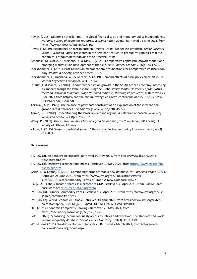
34

Rey, H. (2015). Dilemma not trilemma: The global financial cycle and monetary policy independence. National Bureau of Economic Research, Working Paper, 21162. Retrieved 24 June 2021, from https://www.nber.org/papers/w21162

Reyes, L. (2019). Regímenes de crecimiento en América Latina: Un análisis empírico. Kedge Business

School , Working Paper, presented in the Seminar: Estructura productiva y política macroe-conómica: Enfoques heterodoxos desde América Latina.

Schedelik, M., Nölke, A., Mertens, D., & May, C. (2021). Comparative Capitalism, growth models and emerging markets: The development of the field. New Political Economy, 26(4), 514-526.

Stockhammer, E. (2021). Post-Keynesian macroeconomic foundations for Comparative Political Econ-omy. Politics & Society, advance access, 1-32.

Stockhammer, E., Qazizada, W., & Gechert, S. (2019). Demand effects of fiscal policy since 2008. Re-

view of Keynesian Economics, 7(1), 57–74. Strauss, I., & Isaacs, G. (2016). Labour compensation growth in the South African economy: Assessing

its impact through the labour share using the Global Policy Model. University of the Witwa-

tersrand, National Minimum Wage Research Initiative, Working Paper Series, 4. Retrieved 24 June 2021 from https://nationalminimumwage.co.za/wp-content/uploads/2016/08/NMW-RI-GPM-Model-Final.pdf

Thirlwall, A. P. (1979). The balance of payments constraint as an explanation of the international growth rate differences. PSL Quarterly Review, 32(128), 45–53.

Tomio, B. T. (2020). Understanding the Brazilian demand regime: A Kaleckian approach. Review of

Keynesian Economics, 8(2), 287–302. Wang, P. (2009). Three essays on monetary policy and economic growth in China (PhD Thesis). Uni-

versity of Ottawa, Ottawa. Yılmaz, E. (2015). Wage or profit-led growth? The case of Turkey. Journal of Economic Issues, 49(3),

814–834.

Data sources

BIS (2021a). BIS total credit statistics. Retrieved 10 May 2021, from https://www.bis.org/statis-tics/totcredit.htm

BIS (2021b). Effective exchange rate indices. Retrieved 10 May 2021, from https://www.bis.org/sta-tistics/eer.htm

Gruss, B., & Kebhaj, S. (2019). Commodity terms of trade a new database. IMF Working Paper, 19/21. Retrieved 24 June 2021, from https://www.imf.org/en/Publications/WP/Is-sues/2019/01/24/Commodity-Terms-of-Trade-A-New-Database-46522

ILO (2021). Labour Income Shares as a percent of GDP. Retrieved 30 April 2021, from ILOSTAT data-base website: https://ilostat.ilo.org/data

IMF (2021a). Primary Commodity Prices. Retrieved 30 April 2021, from https://www.imf.org/en/Re-search/commodity-prices

IMF (2021b). World Economic Outlook. Retrieved 30 April 2020, from https://www.imf.org/exter-nal/datamapper/GGXCNL_NGDP@WEO/OEMDC/ADVEC/WEOWORLD

OEC (2021). Economic Complexity Rankings. Retrieved 20 May 2021, from https://oec.world/en/rankings/eci/hs6/hs96

Solt, F. (2020). Measuring income inequality across countries and over time: The standardized world income inequality database. Social Science Quarterly, 101(3), 1183–1199.

World Bank (2021). World Development Indicators. Retrieved 2 March 2021, from https://data-bank.worldbank.org/home.aspx

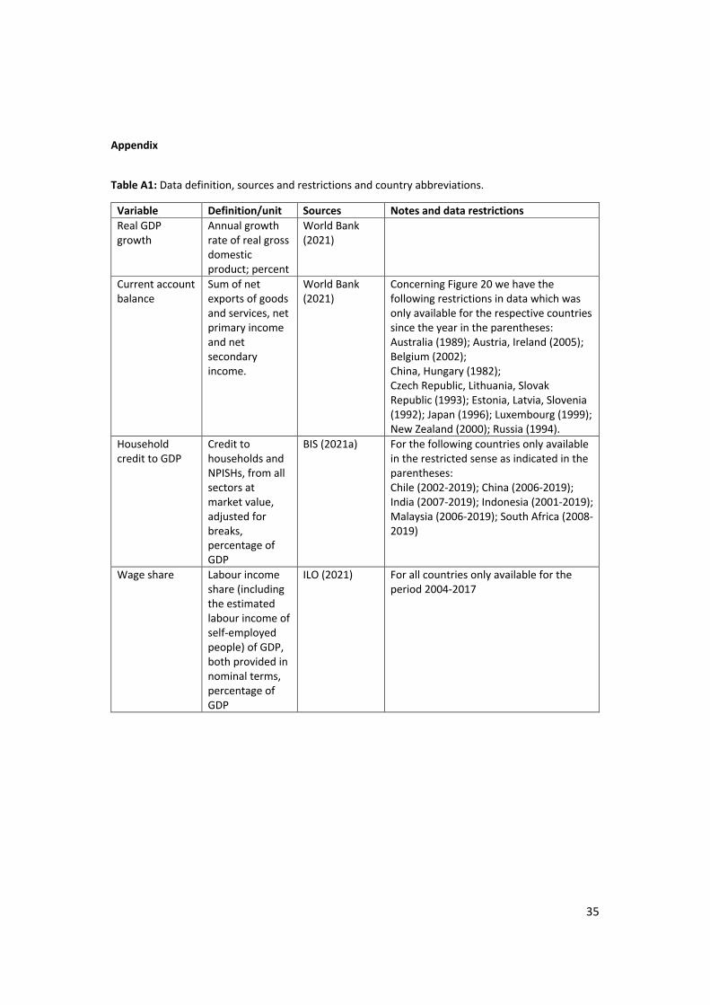
35

Appendix

Table A1: Data definition, sources and restrictions and country abbreviations.

Variable Definition/unit Sources Notes and data restrictions Real GDP growth

Annual growth rate of real gross domestic product; percent

World Bank (2021)

Current account balance

Sum of net exports of goods and services, net primary income and net secondary income.

World Bank (2021)

Concerning Figure 20 we have the following restrictions in data which was only available for the respective countries since the year in the parentheses: Australia (1989); Austria, Ireland (2005); Belgium (2002); China, Hungary (1982); Czech Republic, Lithuania, Slovak Republic (1993); Estonia, Latvia, Slovenia (1992); Japan (1996); Luxembourg (1999); New Zealand (2000); Russia (1994).

Household credit to GDP

Credit to households and NPISHs, from all sectors at market value, adjusted for breaks, percentage of GDP

BIS (2021a) For the following countries only available in the restricted sense as indicated in the parentheses: Chile (2002-2019); China (2006-2019); India (2007-2019); Indonesia (2001-2019); Malaysia (2006-2019); South Africa (2008-2019)

Wage share Labour income share (including the estimated labour income of self-employed people) of GDP, both provided in nominal terms, percentage of GDP

ILO (2021) For all countries only available for the period 2004-2017

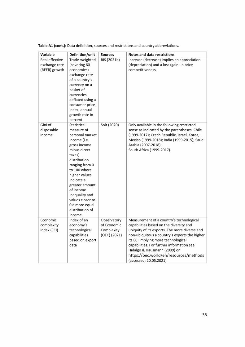
36

Table A1 (cont.): Data definition, sources and restrictions and country abbreviations.

Variable Definition/unit Sources Notes and data restrictions Real effective exchange rate (REER) growth

Trade-weighted (covering 60 economies) exchange rate of a country’s currency on a basket of currencies, deflated using a consumer price index; annual growth rate in percent

BIS (2021b) Increase (decrease) implies an appreciation (depreciation) and a loss (gain) in price competitiveness.

Gini of disposable income

Statistical measure of personal market income (i.e. gross income minus direct taxes) distribution ranging from 0 to 100 where higher values indicate a greater amount of income inequality and values closer to 0 a more equal distribution of income.

Solt (2020) Only available in the following restricted sense as indicated by the parentheses: Chile (1999-2017); Czech Republic, Israel, Korea, Mexico (1999-2018); India (1999-2015); Saudi Arabia (2007-2018); South Africa (1999-2017).

Economic complexity index (ECI)

Index of an economy’s technological capabilities based on export data

Observatory of Economic Complexity (OEC) (2021)

Measurement of a country’s technological capabilities based on the diversity and ubiquity of its exports. The more diverse and non-ubiquitous a country’s exports the higher its ECI implying more technological capabilities. For further information see Hidalgo & Hausmann (2009) or https://oec.world/en/resources/methods (accessed: 20.05.2021).

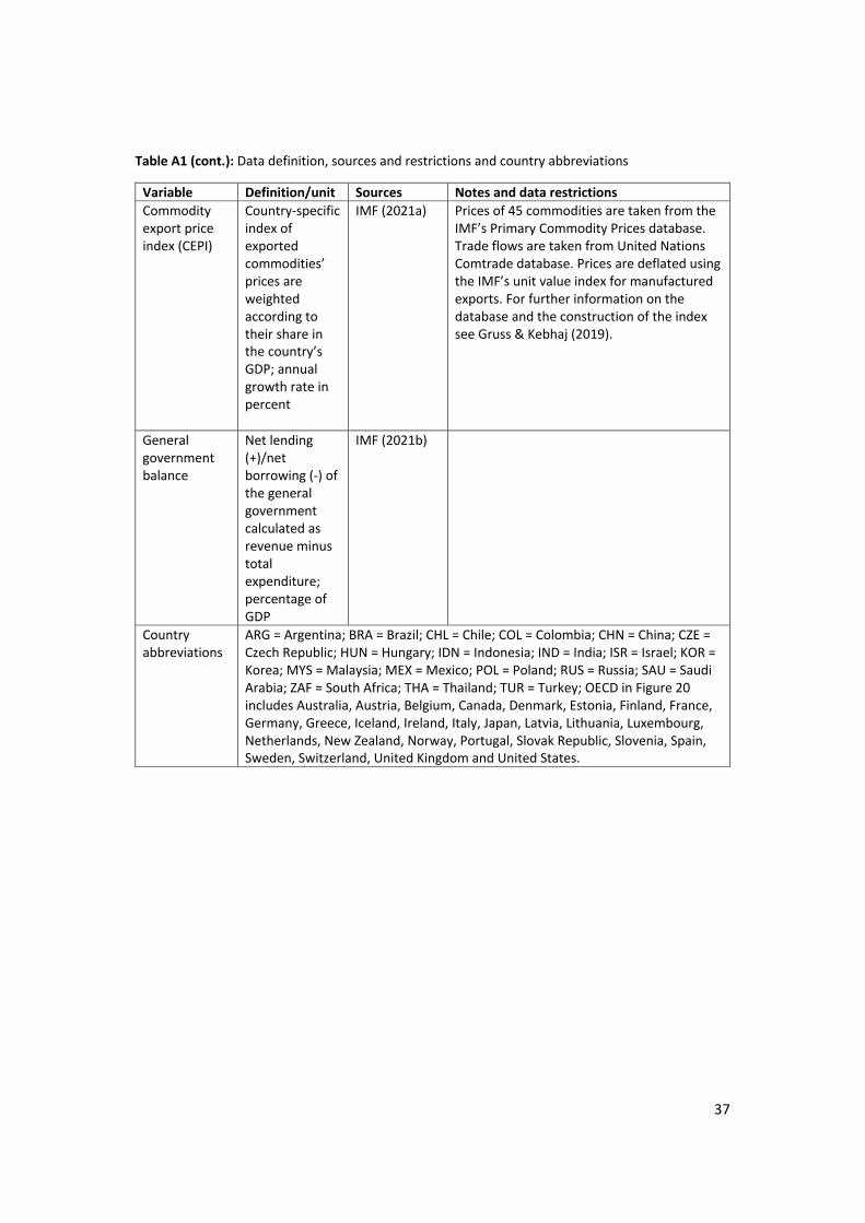
37

Table A1 (cont.): Data definition, sources and restrictions and country abbreviations

Variable Definition/unit Sources Notes and data restrictions Commodity export price index (CEPI)

Country-specific index of exported commodities’ prices are weighted according to their share in the country’s GDP; annual growth rate in percent

IMF (2021a) Prices of 45 commodities are taken from the IMF’s Primary Commodity Prices database. Trade flows are taken from United Nations Comtrade database. Prices are deflated using the IMF’s unit value index for manufactured exports. For further information on the database and the construction of the index see Gruss & Kebhaj (2019).

General government balance

Net lending (+)/net borrowing (-) of the general government calculated as revenue minus total expenditure; percentage of GDP

IMF (2021b)

Country abbreviations

ARG = Argentina; BRA = Brazil; CHL = Chile; COL = Colombia; CHN = China; CZE = Czech Republic; HUN = Hungary; IDN = Indonesia; IND = India; ISR = Israel; KOR = Korea; MYS = Malaysia; MEX = Mexico; POL = Poland; RUS = Russia; SAU = Saudi Arabia; ZAF = South Africa; THA = Thailand; TUR = Turkey; OECD in Figure 20 includes Australia, Austria, Belgium, Canada, Denmark, Estonia, Finland, France, Germany, Greece, Iceland, Ireland, Italy, Japan, Latvia, Lithuania, Luxembourg, Netherlands, New Zealand, Norway, Portugal, Slovak Republic, Slovenia, Spain, Sweden, Switzerland, United Kingdom and United States.

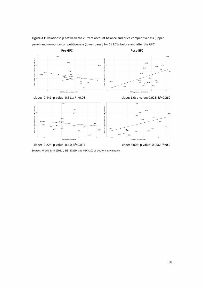
38

Figure A1: Relationship between the current account balance and price competitiveness (upper

panel) and non-price competitiveness (lower panel) for 19 ECEs before and after the GFC.

Pre-GFC Post-GFC

slope: -0.441; p-value: 0.311; R2=0.06 slope: 1.0; p-value: 0.025; R2=0.262


Sources: World Bank (2021), BIS (2021b) and OEC (2021), author’s calculations.

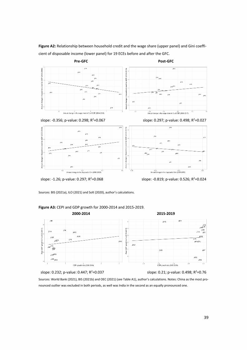
39

Figure A2: Relationship between household credit and the wage share (upper panel) and Gini coeffi-

cient of disposable income (lower panel) for 19 ECEs before and after the GFC.

Pre-GFC Post-GFC


slope: -1.26; p-value: 0.297; R2=0.068 slope: -0.819; p-value: 0.526; R2=0.024

Sources: BIS (2021a), ILO (2021) and Solt (2020), author’s calculations.

Figure A3: CEPI and GDP growth for 2000-2014 and 2015-2019.

Sources: World Bank (2021), BIS (2021b) and OEC (2021) (see Table A1), author’s calculations. Notes: China as the most pro-

nounced outlier was excluded in both periods, as well was India in the second as an equally pronounced one.

2000-2014 2015-2019

slope: 0.232; p-value: 0.447; R2=0.037 slope: 0.21; p-value: 0.498; R2=0.76

Imprint Editors: Sigrid Betzelt, Eckhard Hein (lead editor), Martina Metzger, Martina Sproll, Christina Teipen, Markus Wissen, Jennifer Pédussel Wu, Reingard Zimmer ISSN 1869-6406 Printed by HWR Berlin Berlin October 2021

Growth drivers in emerging capitalist economies before and ...

Documents

Transcript of Growth drivers in emerging capitalist economies before and ...