Growth Dependent Computation of Chokepointsin Metabolic Networks?

Alexandru Oarga1[0000−0002−7271−733X], BridgetBannerman2[0000−0002−5746−8283], and Jorge Julvez1[0000−0002−7093−228X]

1 Department of Computer Science and Systems Engineering, University of Zaragoza,Zaragoza, Spain {718123,julvez}@unizar.es

2 Department of Medicine, University of Cambridge, Cambridge, UKbpc28@cam.ac.uk

Abstract. Bacterial infections are among the major causes of mortal-ity in the world. Despite the social and economical burden produced bybacteria, the number of new drugs to combat them increases very slowlydue to the cost and time to develop them. Thus, innovative approachesto identify efficiently drug targets are required. In the absence of ge-netic information, chokepoint reactions represent appealing drug targetssince their inhibition might involve an important metabolic damage. Incontrast to the standard definition of chokepoints, which is purely struc-tural, this paper makes use of the dynamical information of the modelto compute chokepoints. This novel approach can provide a more realis-tic set of chokepoints. The dependence of the number of chokepoints onthe growth rate is assessed on a number of metabolic networks. A soft-ware tool has been implemented to facilitate the computation of growthdependent chokepoints by the practitioners.

Keywords: Chokepoint Reactions · Metabolic Networks · Petri Nets ·Flux Balance Analysis

1 Introduction

Diseases caused by bacteria are one of the main causes of mortality in both de-veloped and in-development countries. According to the World Health Organisa-tion (WHO) in 2016, tuberculosis was the tenth cause of death worldwide whichmakes its pathogen, Mycobacterium tuberculosis, the infectious agent with thehigher caused mortality. Moreover, upper respiratory system’s diseases causedby microorganisms, like virus and bacteria, were the fourth cause of mortality[20]. In 2010 pneumonia was the leading cause of child mortality causing nearly1.4 million deaths among children younger than 5 years of age [7].

Despite the high mortality caused by bacteria the development of new an-tibiotics is slow and challenging. Furthermore, bacteria have evolved complex

? This work was supported by the Spanish Ministry of Science, Innovation and Univer-sities [ref. Medrese-RTI2018-098543-B-I00], and by the Medical Research Council,UK, MR/N501864/1.

2 A. Oarga et al.

mechanisms which make them difficult to fight. Thus, there is an urgent need todesign novel methods for the development of new drugs. A promising possibilityis to consider basic cellular processes as targets for antibiotic development [12].

Metabolism is the set of basic life processes that take place in the cell, and it isthe means by which cells can maintain life and grow from their environment. Themetabolism of a cell can be represented by a metabolic network that accountsfor all the metabolic reactions that take place in the cell. A possible strategyfor drug discovery is to find and damage critical vulnerabilities of the metabolicnetwork that could stop the growth and replication of the bacteria.

Metabolism as a target has been proven to be an interesting approach inother areas like oncology [9] or viral diseases [10]. A number of methods havebeen proposed in order to find vulnerabilities in the metabolism that may lead totherapeutic results. Some of these methods consider topological properties of themetabolism with the purpose of finding possible critical spots, as for example:determine the importance of a metabolite based on the k-shortest paths betweenmetabolites [15], or consider the inter-reactions dependence to find out how muchinfluence a reaction has on metabolism [16]. Other methods focus on the geneticinformation associated with the metabolism, and compute, for instance, the setof genes that are essential for the survival of the cell [21].

Although a number of genome-scale models (GEMs) have been developedrecently, most of them just account for the stoichiometry of their reactions andlack genetic information. This is usually the case in GEMs of bacteria. Thisdearth of data hampers the analysis of models, namely those based on geneessentiality, and calls for the design of computational methods that exploit asmuch as possible the available biological information. Here, we focus on thecomputation of chokepoints in metabolic networks [18], where a chokepoint isa reaction that is either the only producer or the only consumer of a givenmetabolite. Hence, the inhibition of a chokepoint would lead to the depletion orunlimited accumulation of metabolites, thus, potentially leading to an importantdisruption in the cellular metabolism. Chokepoints are, therefore, appealing drugtargets of the bacterial metabolism.

The current approaches to compute chokepoints are based exclusively on thetopology of the metabolic network and disregard the dynamic information thatmight be available. This dynamic information usually refers to the flux boundsof some metabolic reactions. As it will be shown, ignoring such an informationcan lead to the misidentification of chokepoints. The approach presented in thispaper exploits the available flux bounds and computes, for a given growth rateof the cell, the set of chokepoints of the metabolic network. Such chokepointsare potential drug targets whose inhibition could involve a metabolic burden atthe given growth rate.

The rest of the paper is organized as follows: Section 2 introduces the ba-sic concepts and definition that will be used in the paper. Section 3 describesthe computational method to obtain growth dependent chokepoints. Section 4analyses the relationship between growth rate and number of chokepoints in theGEM of Mycobacterium leprae. The main conclusions of the paper are drawn in

Growth Dependent Computation of Chokepoints in Metabolic Networks 3

section 5. Finally, Appendix A introduces the software tool developed to com-pute growth dependent chokepoints, and Appendix B reports the number ofchokepoints found in the GEMs of different microorganisms.

2 Preliminary concepts and definitions

2.1 Constraint-based models

A constraint-based model [19, 13] is a tuple {R, M, S, lb, ub} where R is aset of reactions, M is a set of metabolites, S ∈ R|M|×|R| is the stoichiometricmatrix, and lb, ub : R → R are lower and upper flux bounds of the reactions.

Each reaction is associated with a set of reactant metabolites and a set ofproduct metabolites (one of these sets can be empty). For instance, the reactionr1 : A→ 2B has one reactant, A, and one product, B. The number 2 expressesthe stoichiometric weight, i.e. two units of B are produced per each unit of Athat is consumed. The stoichiometric matrix S accounts for all the stoichiometricweights of the reactions, i.e. S[m, r] is the stoichiometric weight of metabolitem ∈ M for reaction r ∈ R. Thus, if S[m, r] < 0 then m is consumed when roccurs; if S[m, r] > 0 then m is produced when r occurs; and if S[m, r] = 0 thenm is neither consumed nor produced when r occurs.

Constraint-based models can be represented graphically as Petri nets [11,5] where places, which are drawn as circles, are associated with metabolites,and transitions, which are drawn as rectangles, are associated with reactions.An arc from a place(transition) to a transition(place) means that the place isa reactant(product). The weights of the arcs of the Petri net correspond to thestoichiometric weights, in other words, the stoichimetric matrix of a constraint-base model and the incidence matrix of its corresponding Petri net coincide.

Example 1. The Petri net in Figure 1 represents a simple contraint-based modelthat consists of 13 reactions and 9 metabolites. As an example, transition r6models the reaction r6 : ma → 2md.

2.2 Topological definitions.

Borrowing the usual Petri net notation (given a node x of a Petri net, •x andx• denote the sets of the input and output nodes of x respectively), we definethe following sets for constraint-based models:

– Set of products of r: r• = {m ∈M|S(m, r) > 0}– Set of reactants of r: •r = {m ∈M|S(m, r) < 0}– Set of consumers of m: m• = {r ∈ R|S(m, r) < 0}– Set of producers of m: •m = {r ∈ R|S(m, r) > 0}

A chokepoint is a reaction that is the only producer or the only consumer ofa metabolite. More formally:

4 A. Oarga et al.

r1:lb=0, ub=10 r2:lb=0, ub=10

ma

mb mc

r3:lb=0, ub=0 r4:lb=0, ub=100 r5:lb=0, ub=100

r6:lb=0, ub=100 r7:lb=0, ub=100 r8:lb=−100, ub=100

md me

r9:lb=−100, ub=100

r10:lb=−100, ub=100

r11:lb=0, ub=100

mf mg

mh

r12:lb=0, ub=100

mi

r13:lb=0, ub=100

2

2

Fig. 1: Petri net modelling a constraint-based model. The values lb and ub arethe lower and upper flux bounds of reactions. Non-reversible reactions are repre-sented by simple rectangles, reversible reactions by double rectangles and dead-reactions by rectangles with a cross.

Definition 1. A reaction r ∈ R is a chokepoint if there exists m ∈M such thatm• = {r} or •m = {r}.

The set of chokepoint reactions will be denoted as CP . Notice that theinhibition of the enzymes associated with a chokepoint will lead either to thedepletion of metabolites (which might be essential for the cell) if the chokepointis the only producer, or to the indefinite accumulation of metabolites (whichwill not be used as expected or might be toxic) if the chokepoint is the onlyconsumer. Thus, a chokepoint is an attractive drug target because in both cases,essential functions of the cell can be affected by its inhibition [18].

A dead-end metabolite (DEM) is a metabolite that lacks either producing orconsuming reactions:

Growth Dependent Computation of Chokepoints in Metabolic Networks 5

Definition 2. A metabolite m ∈M is a dead-end metabolite (DEM) if m• = {}or •m = {}.

The presence of a DEM in the network reflects an incompleteness in themodel, which might require further curation [8].

Example 2. In the Petri net in Figure 1, r1 is a producer of ma, i.e. r1 ∈ •ma;r4 is a chokepoint because it is the only producer of mc, i.e. {r4} = •mc andr4 ∈ CP ; and mh is a dead-end metabolite, i.e. mh ∈ DEM .

2.3 Flux dependent definitions.

The functions lb and ub establish lower and upper steady state flux boundson the reactions, where flux is the rate of turnover of molecules through thereaction. These functions must satisfy that lb(r) ≤ ub(r) for every r ∈ R. Lowerand upper bounds provide useful information about the system and might alterthe sets of consumer and producer reactions previously defined. Such boundswill be used in the following to improve the analysis of constraint-based models.

In contrast to Petri nets, these bounds can be negative, and hence, the fluxof a reaction can also be negative. A negative flux implies that the metaboliteson the left-hand side of the reaction (which in principle are ”reactants”) areproduced, and the metabolites on the right-hand side of the reaction (which inprinciple are ”products”) are consumed. A reaction whose flux can be both neg-ative and positive is called reversible. Functions lb and ub will be used to definethe sets of flux dependent reversible reactions (RRd), dead reactions (DRd), andnon-reversible reactions (NRd), where the subindex d indicates that the sets areflux dependent :

Definition 3. A reaction r ∈ R is reversible if lb(r) < 0 < ub(r).

The set of reversible reactions is denoted RRd, i.e. RRd = {r ∈ R| r isreversible}.

Definition 4. A reaction r ∈ R is dead if lb(r) = ub(r) = 0.

The set of dead reactions is denoted DRd, i.e. DRd = {r ∈ R| r is dead}.

Definition 5. A reaction r ∈ R is non-reversible if (0 ≤ lb(r) ∧ 0 < ub(r)) ∨(lb(r) < 0 ∧ ub(r) ≤ 0).

The set of non-reversible reactions is denoted NRd, i.e. NRd = {r ∈ R| r isnon-reversible }.

Clearly, the sets RRd, DRd and NRd partition the set of reactions R, i.e.RRd ∪DRd ∪NRd = R, RRd∩DRd = ∅, DRd∩NRd = ∅, and RRd∩NRd = ∅.

Non-reversible, reversible and dead reactions will be represented graphicallyas rectangles, double rectangles, and rectangles with a cross inside respectively.

Example 3. In Figure 1, the above defined sets are: RRd = {r8, r9 r10}, DRd ={r3}, and NRd = {r1, r2, r4, r5, r6, r7, r11, r12, r13}.

6 A. Oarga et al.

Given that, in constraint-based models, reactions can be reversible or canproceed only backwards, i.e. lb(r) ≤ ub(r) < 0, the concepts related to theconsumption and production of metabolites must be revisited. Thus, new sets ofreactants, products, consumers, and producers which take into account the fluxbounds are defined as follows:

– Set of products of r:r•d = {m ∈M|(S(m, r) > 0 ∧ ub(r) > 0) ∨ (S(m, r) < 0 ∧ lb(r) < 0)}

– Set of reactants of r:•rd = {m ∈M|(S(m, r) < 0 ∧ ub(r) > 0) ∨ (S(m, r) > 0 ∧ lb(r) < 0)}

– Set of consumers of m:m•d = {r ∈ R|(S(m, r) < 0 ∧ ub(r) > 0) ∨ (S(m, r) > 0 ∧ lb(r) < 0)}

– Set of producers of m:•md = {r ∈ R|(S(m, r) > 0 ∧ ub(r) > 0) ∨ (S(m, r) < 0 ∧ lb(r) < 0)}

Flux dependent definitions of chokepoints and dead-end metabolites can bewritten as:

Definition 6. A reaction r ∈ R is a flux dependent chokepoint if there existsm ∈M such that m•d = {r} or •md = {r}.

Definition 7. A metabolite m ∈ M is a flux dependent dead-end metabolite ifm•d = {} or •md = {}.

The sets of flux dependent chokepoint reactions and dead-end metaboliteswill be denoted as CPd and DEMd respectively.

Example 4. In Figure 1, r12 is a flux dependent chokepoint, i.e. r12 ∈ CPd; andmh is a flux dependent dead-end metabolite, i.e. mh ∈ DEMd.

3 Growth dependent chokepoints

In GEMs, unknown flux bounds are given default values, e.g.lb(r) = −1000 mmol g−1h−1 and ub(r) = 1000 mmol g−1h−1 (recall thatflux bounds establish the direction in which the reaction can proceed). Thus,all the reactions that are given default values are considered as reversible.However, not all the fluxes in the ranges given by the flux bounds of GEMsmodels are compatible with a positive growth rate. By using Flux BalanceAnalysis (FBA)[14] and Flux Variability Analysis (FVA)[4] it is possible toobtain tighter flux bounds for a given growth rate. Such tighter bounds couldimply that, reactions which were initially considered as reversible, are in factnon-reversible for the given growth rate. This might alter the original set ofchokepoints, i.e. the set of chokepoints depend on the growth rate. This sectiondescribes how growth dependent chokepoints can be computed.

Flux Balance Analysis (FBA) is a mathematical procedure for the estimationof steady state fluxes in constraint-based models. FBA can be used, for instance,to predict the growth rate of an organism or the rate of production of a given

Growth Dependent Computation of Chokepoints in Metabolic Networks 7

metabolite. Mathematically, FBA is expressed as a linear programming problemthat maximises an objective function subject to steady state constraints. In thecase of estimating the growth rate, the objective function is biomass production,a reaction that defines the ratios at which metabolites are converted into basicconstituents of the cell as nucleic acids or proteins [14].

Let v ∈ R|R| be the vector of fluxes of reactions and v[r] denote the flux ofreaction r. At steady state, it holds that S · v = 0, where S is the stoichiometricmatrix. The steady state fluxes of reactions are also lower and upper boundedby lb and ub. Thus, the FBA linear programming problem is:

max z · vst. S · v = 0

lb(r) ≤ v[r] ≤ ub(r) ∀r ∈ R(1)

where z ∈ R|R| expresses the objective function.It is a common assumption that the metabolism of prokaryotes has evolved

to maximize the growth of the cells. Hence, the growth rate given by the biomassproduction is an empirically reasonable choice for the objective function of FBAapplied to bacteria [17].

A given growth, i.e. a given flux through the reaction modelling biomassproduction, can be achieved by different fluxes of the reactions. This means thateach reaction can have a range of fluxes that is compatible with a given growth.Flux Variability Analysis (FVA) can be used to compute such range of fluxes foreach reaction. [2].

More precisely, FVA[4] is a mathematical procedure to compute the mini-mum and maximum fluxes of reactions that are compatible with some state,e.g. supporting 90% of the maximum growth yielded by FBA. Among other ap-plications, FVA can be used to study the network flexibility, and studying thenetwork response under suboptimal conditions.

Let µmax be the maximum growth calculated by FBA. FVA is computed bysolving two independent linear programming problems per reaction r ∈ R. Oneprogramming problem maximizes the flux of r, v[r], and the other minimizesv[r]. The constraints of both problems are the same: the steady state conditionS · v = 0, the flux bounds lb(r) ≤ v[r] ≤ ub(r), and the maintenance of theoptimum value given by FBA to a certain degree. This last constraint is expressedas γ · µmax ≤ z · v where z is the same vector as in (1) and γ ∈ [0, 1] representsthe fraction of optimal value that must be satisfied. Thus, the two programmingproblems for a given reaction r ∈ R can be expressed as:

max /min v[r]

st. S · v = 0

lb(r) ≤ v[r] ≤ ub(r) ∀r ∈ Rγ · µmax ≤ z · v

(2)

Let lbγ , ubγ : R → R be the result of running FVA on a constraint-basedmodel {R, M, S, lb, ub} for a given γ. If the flux bounds lb, ub of the

8 A. Oarga et al.

constrained-based model are replaced by lbγ , ubγ , a new constraint-based model,{R, M, S, lbγ , ubγ}, with more constrained flux bounds is obtained.

Given γ, the sets of flux dependent products, reactants, consumers, and pro-ducers of the model {R, M, S, lbγ , ubγ} are denoted as r•γ ,

•rγ ,m•γ ,•mγ respec-

tively. Similarly, the sets of flux dependent reversible reactions, dead reactions,and non-reversible reactions are denoted as RRγ , DRγ , NRγ respectively. Thesets of flux dependent chokepoint reactions and dead-end metabolites are de-noted as CPγ and DEMγ .

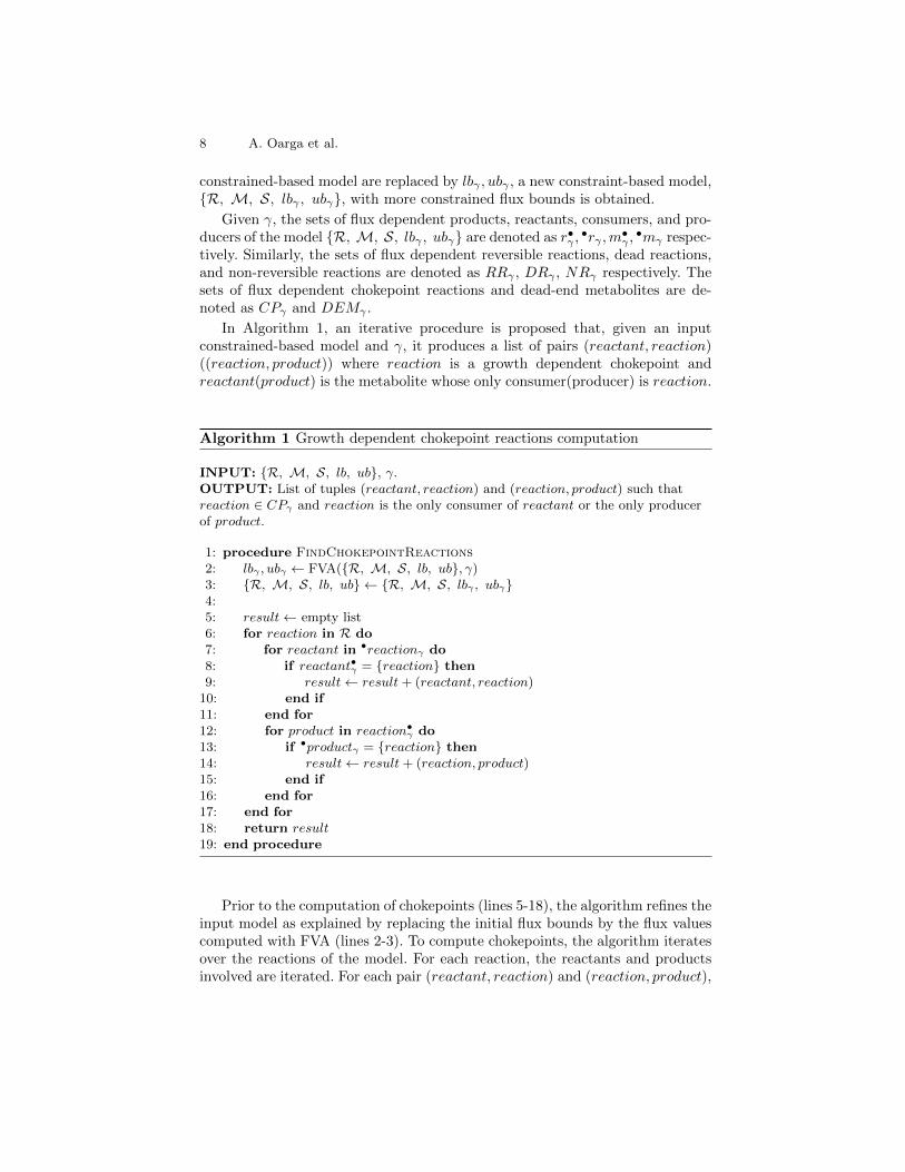
In Algorithm 1, an iterative procedure is proposed that, given an inputconstrained-based model and γ, it produces a list of pairs (reactant, reaction)((reaction, product)) where reaction is a growth dependent chokepoint andreactant(product) is the metabolite whose only consumer(producer) is reaction.

Algorithm 1 Growth dependent chokepoint reactions computation

INPUT: {R, M, S, lb, ub}, γ.OUTPUT: List of tuples (reactant, reaction) and (reaction, product) such thatreaction ∈ CPγ and reaction is the only consumer of reactant or the only producerof product.

1: procedure FindChokepointReactions2: lbγ , ubγ ← FVA({R, M, S, lb, ub}, γ)3: {R, M, S, lb, ub} ← {R, M, S, lbγ , ubγ}4:5: result← empty list6: for reaction in R do7: for reactant in •reactionγ do8: if reactant•γ = {reaction} then9: result← result+ (reactant, reaction)

10: end if11: end for12: for product in reaction•

γ do13: if •productγ = {reaction} then14: result← result+ (reaction, product)15: end if16: end for17: end for18: return result19: end procedure

Prior to the computation of chokepoints (lines 5-18), the algorithm refines theinput model as explained by replacing the initial flux bounds by the flux valuescomputed with FVA (lines 2-3). To compute chokepoints, the algorithm iteratesover the reactions of the model. For each reaction, the reactants and productsinvolved are iterated. For each pair (reactant, reaction) and (reaction, product),

Growth Dependent Computation of Chokepoints in Metabolic Networks 9

if Definition 6 is satisfied, the reaction is considered a chokepoint reaction withthe given metabolite.

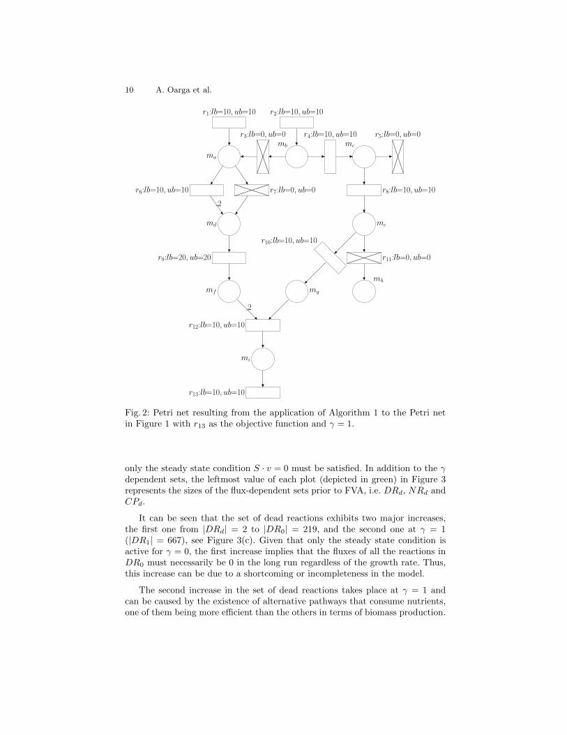
Example 5. Let us assume that r13 in Figure 1 represents growth, i.e. the compo-nent of z in (1) that corresponds to r13 is equal to 1 and the rest of componentsof z are 0. Let us also assume that it is desired to assess the directionality ofthe reactions and compute the set of chokepoints when the growth is maximum.This can be achieved by applying Algorithm 1 with γ = 1. The new flux boundsyielded by the algorithm are shown in Figure 2.

As a result of the new flux bounds given to the model, reactions r5, r7and r11 become dead reactions, i.e. r5, r7, r11 ∈ DR1, and reactions r8, r9, r10,which where reversible reactions in Figure 1, become non-reversible reactions,i.e. r8, r9, r10 ∈ NR1. This change in the directionality of the reactions involveschanges in the set of flux-dependent chokepoints, in particular r6 becomes achokepoint, i.e. r6 ∈ CP1, and r11, which was a chokepoint in Figure 1, becomesa dead-reaction, i.e. r11 ∈ DR1.

4 Chokepoint Analysis

The computation of flux bounds by means of FVA can be carried out with anoptimal state, i.e. γ = 1 in (2), or with suboptimal states, i.e. 0 ≤ γ < 1. Whilein an optimal state all the fluxes must be optimally directed towards growth, insuboptimal states fluxes are allowed to be diverted towards other functionalities.This section analyses the impact of γ in the sets of reversible, non-reversible,dead and chokepoint reactions of a constraint-based model. To achieve this goalthe flux bounds of the model will be refined according to different values of γand the mentioned sets of reactions will be computed.

All the results presented in this section have been obtained by a softwaretool which implements Algorithm 1 and computes the sets RRγ , DRγ , NRγ andCPγ . A description of the tool can be found in Appendix A. The tool has beenexecuted on a number of constraint-based models yielding the results presentedin Appendix B.

4.1 Case study: Mycobacterium leprae

This subsection presents the results obtained for the constraint-based model ofthe in vivo GEM of M. leprae [1, 6]. This model is composed of 998 metabo-lites and 1228 reactions. The sizes of the flux-dependent sets of reactions are|RRd|=288, |NRd|=938, |DRd|=2, and the number of flux-dependent CP is|CPd| = 667. In order to assess the dependence of these sets on γ, the fluxbounds of the model have been refined for different values of γ in the interval[0, 1].

Figure 3 shows the sizes of the sets DRγ , NRγ and CPγ , in plot (a), (b) and(c) respectively, for different values of γ. Notice that if γ = 0 then the constraintγ · µmax ≤ z · v in (2) does not impose a minimum growth on the model, and

10 A. Oarga et al.

r1:lb=10, ub=10 r2:lb=10, ub=10

ma

mb mc

r3:lb=0, ub=0 r4:lb=10, ub=10 r5:lb=0, ub=0

r6:lb=10, ub=10 r7:lb=0, ub=0 r8:lb=10, ub=10

md me

r9:lb=20, ub=20

r10:lb=10, ub=10

r11:lb=0, ub=0

mf mg

mh

r12:lb=10, ub=10

mi

r13:lb=10, ub=10

2

2

Fig. 2: Petri net resulting from the application of Algorithm 1 to the Petri netin Figure 1 with r13 as the objective function and γ = 1.

only the steady state condition S · v = 0 must be satisfied. In addition to the γdependent sets, the leftmost value of each plot (depicted in green) in Figure 3represents the sizes of the flux-dependent sets prior to FVA, i.e. DRd, NRd andCPd.

It can be seen that the set of dead reactions exhibits two major increases,the first one from |DRd| = 2 to |DR0| = 219, and the second one at γ = 1(|DR1| = 667), see Figure 3(c). Given that only the steady state condition isactive for γ = 0, the first increase implies that the fluxes of all the reactions inDR0 must necessarily be 0 in the long run regardless of the growth rate. Thus,this increase can be due to a shortcoming or incompleteness in the model.

The second increase in the set of dead reactions takes place at γ = 1 andcan be caused by the existence of alternative pathways that consume nutrients,one of them being more efficient than the others in terms of biomass production.

Growth Dependent Computation of Chokepoints in Metabolic Networks 11

0 0.5 1

600

800

1,000

γ

|NRγ|

Non-Reversible Reactions

(a)

0 0.5 1

500

600

700

γ

|CPγ|

Chokepoint Reactions

(b)

0 0.5 1

0

200

400

600

γ

|DRγ|

Dead Reactions

(c)

Fig. 3: Sizes of the sets of reactions DRγ , NRγ and CPγ of M. leprae forγ ∈ [0, 1]. The leftmost value of each plot corresponds to DRd, NRd and CPdrespectively.

The next subsection proposes simplified models that illustrate how these suddenincreases take place.

With respect to chokepoints, see Figure 3(b), the number of flux-dependentchokepoints is |CPd| = 668. This number increases to |CP0| = 733 when thesteady state constraint is forced, and increases slowly with γ, at γ = 0.9 itholds |CP0.9| = 741. That is, Algorithm 1 identifies more chokepoints than theones that are present originally in the model. The sudden drop of chokepoints atγ = 1, |CP1| = 469, is due to the fact that at the optimal state many chokepointsbecome dead reactions as discussed previously.

In a similar way to the set of chokepoints, the number of non-reversiblereactions increases slowly with γ and it falls abruptly at γ = 1 . This means thatthe sets NRγ and CPγ decrease at the optimal state as many of these reactionsbecome dead reactions.

Figure 4 presents a Sankey diagram showing how reactions are distributedamong the sets NR, RR and DR and the flow of transformations that takes placeamong these sets from the initial model to a model refined with a suboptimalstate of γ = 0.9, and from this suboptimal state model to an optimal state modelrefined with γ = 1.0. Notice that at γ = 1.0 the set of dead reactions becomes thelargest set of reactions, and that the set of reversible reactions is vastly reducedat both suboptimal and optimal growth.

As it is reported in Appendix B, similar trends to the ones discussed here forthe sets NR, DR and CP are exhibited by other models.

4.2 Dead reactions and growth rate

It has been shown that refining a model with a suboptimal growth can cause theset of dead reactions,DR, to increase, and also that this set increases further withan optimal growth refinement. These changes in DR are caused by particularnetwork structures that can appear in a metabolic network. This subsection

12 A. Oarga et al.

Fig. 4: Sankey diagram showing the dependence of the sets NR, RR and DR onthe growth rate.

illustrates through an abstract model the types of structures that can producesuch changes in DR.

Let us consider the constraint-based model depicted as a Petri net in Figure 5.The lower and upper flux bounds of the model are reported in Table 1 of thefigure. According to such flux bounds all the reactions are non-reversible, i.e.DR = {}, see column type. The exchange reactions are r1 and r10, which couldmodel nutrient uptake and secretion of a metabolite respectively. The reactionmodelling biomass production is r7, i.e. the flux of r7 represents the growthrate of system being modelled. Hence, the objective funcion of FBA, see (1),is the maximization of v[r7]. For the given net structure and flux bounds, themaximum growth rate yielded by FBA (1) is µmax = 200.

Table 2 reports the refined flux bounds and the type of each reaction forγ = 0, γ = 0.9 and γ = 1. If γ = 0 then only the steady state constraint,S · v = 0, of FVA (2) is taken into account to compute the refined flux bounds.Thus, any possible steady state must satisfy the bounds, lb0 and ub0, of the rowsassociated with γ = 0. For such γ, all the lower bounds, lb0, are kept to 0 andthe upper bounds, ub0, are constrained by the upper flux bound of r1 which isub(r1) = 100. It should be noted that ub0(r8) = ub0(r9) = ub0(r10) = 0, that isreactions r8, r9 and r10 are dead at any steady state, i.e. DR0 = {r8, r9, r10}.

Recall that this increase in the number of dead reactions, DR0, also tookplace in the previous subsection for the M. leprae model. The reason why r8becomes dead is because it is producing a DEM mg, if the flux of r8 was positivethen the concentration of mg would increase indefinitely which contradicts theexistence of a steady state.

Let us now focus on r9 and r10. The steady state condition, S · v = 0, formetabolite mh imposes v[r9] = v[r10] (i.e. input flux = output flux), whilefor mi the steady state condition is 2 · v[r9] = v[r10] (see weight 2 in the arc

Growth Dependent Computation of Chokepoints in Metabolic Networks 13

r1

ma

r2

mb

r3

r9

mh mi

r10

r4 mc

r5

mfr8 mg

md

r6

me

r72

2

Table 1: Initial flux boundsr lb(r) ub(r) typer1 0.0 100.0 NRr2 0.0 1000.0 NRr3 0.0 1000.0 NRr4 0.0 1000.0 NRr5 0.0 1000.0 NRr6 0.0 1000.0 NRr7 0.0 1000.0 NRr8 0.0 1000.0 NRr9 0.0 1000.0 NRr10 0.0 1000.0 NR

Table 2: Refined model fluxbounds

γ r lbγ(r) ubγ(r) type0.0 r1 0.0 100.0 NR

r2 0.0 100.0 NRr3 0.0 100.0 NRr4 0.0 100.0 NRr5 0.0 200.0 NRr6 0.0 200.0 NRr7 0.0 200.0 NRr8 0.0 0.0 DRr9 0.0 0.0 DRr10 0.0 0.0 DR

0.9 r1 90.0 100.0 NRr2 0.0 20.0 NRr3 0.0 20.0 NRr4 80.0 100.0 NRr5 160.0 200.0 NRr6 180.0 200.0 NRr7 180.0 200.0 NRr8 0.0 0.0 DRr9 0.0 0.0 DRr10 0.0 0.0 DR

1.0 r1 100.0 100.0 NRr2 0.0 0.0 DRr3 0.0 0.0 DRr4 100.0 100.0 NRr5 200.0 200.0 NRr6 200.0 200.0 NRr7 200.0 200.0 NRr8 0.0 0.0 DRr9 0.0 0.0 DRr10 0.0 0.0 DR

Fig. 5: Petri net illustrating the evolution of dead reactions at γ = 0 and γ = 1.

(r9,mi). The only fluxes that satisfy these two conditions simultaneously arev[r9] = v[r10] = 0, i.e. the reactions are dead at any steady state.

At γ = 0.9, the flux of r7 (biomass production) must be at least 0.9 ·µmax =180. Notice that, although DR0 = DR0.9, the lower bounds of some reactions arehigher at γ = 0.9 than at γ = 1, and the upper bounds of some other reactionsare lower at γ = 0.9 than at γ = 1. In general it holds:

ub0.9[r]− lb0.9[r] ≥ ub1[r]− lb1[r] ∀r ∈ R

In other words, the range of steady state fluxes allowed for each reaction de-creases with γ. This is due to the existence of alternative paths in the metabolicnetwork. In the present example, there are two alternative pathways to biomassproduction, namely p1 = (r1, r2, r3, r6, r7) and p2 = (r1, r4, r5, r6, r7). Noticethat p2 is more advantageous than p1 for biomass production as 2 metabolitesmc are produced per each metabolite ma. Thus, near optimal solutions will tendto exploit p2 instead of p1. This implies strictly positive lower bounds, lb0.9, forall the reactions in p2, and decreased upper bounds, ub0.9, for the reactions thatbelong exclusively to p1, i.e. r2 and r3.

14 A. Oarga et al.

The interval [lbγ [r], ubγ [r]] shrinks for every reaction r ∈ R as γ increases,and at γ = 1 the intervals become points. Moreover, at γ = 1 only the mostfavourable path p2 can be used, and hence reactions r2 and r3 become dead.This type of phenomenon causes the sudden increase of DR1 in the M. lepraemodel of the previous subsection.

5 Conclusions

This work has introduced a computational method to incorporate dynamic in-formation, namely flux bounds, in the computation of chokepoints in metabolicnetworks expressed as constraint-based models. The goal behind this approach isto obtain more realistic chokepoints, which are known to be potential drug tar-gets, than those based only on the net topology. Given that flux bounds dependon the growth rate of the organism, the concept of growth dependent choke-points has been defined and an algorithm to compute such chokepoints has beendesigned.

It was found that the number of chokepoints was seriously affected by thenumber of dead reactions, i.e. by reactions with null lower and upper flux bounds.Although the number of dead reactions is not relevant in most of the originalmodels, this number increases significantly when dynamic information is ac-counted for. A major increase takes place when the steady state constraint isenforced on the metabolic network, i.e. at γ = 0. As discussed in subsection 4.2,we hypothesize that such an increase is a sign of some incompleteness in themodel such as the existence of dead-end metabolites, or to missing reactionsthat lead to the incompatibility of positive fluxes with the network stoichiom-etry. Another major increase of dead reactions takes place when the growthrate is maximum, i.e. at γ = 1. At such a rate, all the flux is diverted towardsthe optimal paths for biomass production, and hence, the fluxes of non-optimalalternative paths leading to biomass production and other non-essential pathsbecome 0, i.e. such paths contain dead reactions at γ = 1. Thus, in this case deadreactions might indicate the existence of alternative, or redundant, paths leadingto biomass production. Notice that such redundant paths have the potential tomake the metabolism more robust to attacks.

The protocol for chokepoint computation presented on this paper can re-duce the time spent identifying drug targets in the process of drug discovery.Drug discovery is a time-consuming process, which involves the identificationand validation of drug targets, optimisation, lead discovery and testing beforethe production of drug candidates. Our protocol can contribute reducing the drugtarget identification time by prioritising the selection of potential top targets ofthe pathogenic organism for subsequent validation and optimisation protocolsof the drug discovery process.

References

1. Bannerman, B.P., Vedithi, S.C., Julvez, J., Torres, P., Waman, V.P., Munir, A.,Mendes, V., Malhotra, S., Skwark, M.J., Oliver, S.G., Blundell, T.L.: Analysis

Growth Dependent Computation of Chokepoints in Metabolic Networks 15

of metabolic pathways in mycobacteria to aid drug-target identification. bioRxiv(2019). https://doi.org/10.1101/535856

2. Burgard, A.P., Vaidyaraman, S., Maranas, C.D.: Minimal reaction setsfor escherichia coli metabolism under different growth requirements anduptake environments. Biotechnology progress 17(5), 791–797 (2001).https://doi.org/10.1021/bp0100880

3. Glont, M., Nguyen, T.V.N., Graesslin, M., Halke, R., Ali, R., Schramm, J.,Wimalaratne, S.M., Kothamachu, V.B., Rodriguez, N., Swat, M.J., et al.: Biomod-els: expanding horizons to include more modelling approaches and formats. Nucleicacids research 46(D1), D1248–D1253 (2018). https://doi.org/10.1093/nar/gkx1023

4. Gudmundsson, S., Thiele, I.: Computationally efficient flux variability analysis.BMC Bioinformatics 11(1), 489 (sep 2010). https://doi.org/10.1186/1471-2105-11-489

5. Heiner, M., Gilbert, D., Donaldson, R.: Petri nets for systems and synthetic biology.vol. 5016, pp. 215–264 (06 2008). https://doi.org/10.1007/978-3-540-68894-5 7

6. Karp, P.D., Billington, R., Caspi, R., Fulcher, C.A., Latendresse, M., Kothari,A., Keseler, I.M., Krummenacker, M., Midford, P.E., Ong, Q., Ong, W.K.,Paley, S.M., Subhraveti, P.: The BioCyc collection of microbial genomes andmetabolic pathways. Briefings in Bioinformatics 20(4), 1085–1093 (08 2017).https://doi.org/10.1093/bib/bbx085

7. Lamberti, L.M., Zakarija-Grkovic, I., Fischer Walker, C.L., Theodoratou, E., Nair,H., Campbell, H., Black, R.E.: Breastfeeding for reducing the risk of pneumoniamorbidity and mortality in children under two: A systematic literature review andmeta-analysis (2013). https://doi.org/10.1186/1471-2458-13-S3-S18

8. Mackie, A., Keseler, I.M., Nolan, L., Karp, P.D., Paulsen, I.T.: Dead End Metabo-lites - Defining the Known Unknowns of the E. coli Metabolic Network. PLoS ONE8(9), e75210 (sep 2013). https://doi.org/10.1371/journal.pone.0075210

9. Mazurek, S.: Pyruvate kinase type M2: A key regulator of the metabolic budgetsystem in tumor cells. International Journal of Biochemistry and Cell Biology43(7), 969–980 (jul 2011). https://doi.org/10.1016/j.biocel.2010.02.005

10. Munger, J., Bennett, B.D., Parikh, A., Feng, X.J., McArdle, J., Rabitz, H.A.,Shenk, T., Rabinowitz, J.D.: Systems-level metabolic flux profiling identifies fattyacid synthesis as a target for antiviral therapy. Nature Biotechnology 26(10), 1179–1186 (oct 2008). https://doi.org/10.1038/nbt.1500

11. Murata, T.: Petri Nets: Properties, Analysis and Applications. Procs. of the IEEE77(4), 541–580 (1989). https://doi.org/10.1109/5.24143

12. Murima, P., McKinney, J.D., Pethe, K.: Targeting bacterial central metabolism fordrug development (nov 2014). https://doi.org/10.1016/j.chembiol.2014.08.020

13. Orth, J.D., Conrad, T.M., Na, J., Lerman, J.A., Nam, H., Feist, A.M.,Palsson, B.Ø.: A comprehensive genome-scale reconstruction of Es-cherichia coli metabolism–2011. Molecular Systems Biology 7(1) (2011).https://doi.org/10.1038/msb.2011.65

14. Orth, J.D., Thiele, I., Palsson, B.O.: What is flux balance analysis? (mar 2010).https://doi.org/10.1038/nbt.1614

15. Rahman, S.A., Schomburg, D.: Observing local and global properties ofmetabolic pathways: ’load points’ and ’choke points’ in the metabolicnetworks. Bioinformatics (Oxford, England) 22(14), 1767–74 (jul 2006).https://doi.org/10.1093/bioinformatics/btl181

16. Raman, K., Vashisht, R., Chandra, N.: Strategies for efficient disruption ofmetabolism in Mycobacterium tuberculosis from network analysis. MolecularbioSystems 5(12), 1740–51 (dec 2009). https://doi.org/10.1039/B905817F

16 A. Oarga et al.

17. Segre, D., Vitkup, D., Church, G.M.: Analysis of optimality in natural and per-turbed metabolic networks. Proceedings of the National Academy of Sciences99(23), 15112–15117 (2002). https://doi.org/10.1073/pnas.232349399

18. Singh, S., Malik, B.K., Sharma, D.K.: Choke point analysis of metabolic pathwaysin E.histolytica: A computational approach for drug target identification. Bioin-formation 2(2), 68–72 (aug 2007). https://doi.org/10.6026/97320630002068

19. Varma, A., Palsson, B.Ø.: Metabolic Flux Balancing: Basic Concepts, Scien-tific and Practical Use. Nature Biotechnology 12(10), 994–998 (Oct 1994).https://doi.org/10.1038/nbt1094-994

20. WHO: WHO — Causes of death. WHO (2018)

21. Zhang, R., Lin, Y.: DEG 5.0, a database of essential genes in both prokary-otes and eukaryotes. Nucleic Acids Research 37(suppl 1), D455–D458 (10 2008).https://doi.org/10.1093/nar/gkn858

A Appendix

The software tool findCPcli developed in this work consists of a command lineapplication that, given an input model provided by the user, computes the sizesof the sets of non-reversible reactions, reversible reactions, dead reactions andchokepoint reactions for different values of γ. The results are saved in a spread-sheet file with a format similar to the one presented in Table 3.

The tool findCPcli is distributed as a Python package and requires Python 3.5or a higher version. The source can be found at github.com/findCP/findCPcli.findCPcli can be installed with the pip package management tool:

pip install findCPcli

Once installed, the results for a given SBML model can be computed running:

findCPcli -i <input file> -cp <output file>

, where:

– <input file> is the path of the input SBML model file to be used. Thesupported file formats are .xml, .json and .yml.

– <output file> is the path of the spreadsheet file that will be saved with theresults computed on the model. The available file formats for the spreadsheetfile are .xls, .xlsx and .ods.

When the above command is executed, the command line application willinform about the task that will be computed. If the task finishes successfullyand the spreadsheet file has been saved, the application will inform about it andwill end the execution.

Further information about the operations provided by the application can befound by executing: findCPcli -h .

Growth Dependent Computation of Chokepoints in Metabolic Networks 17

B Appendix

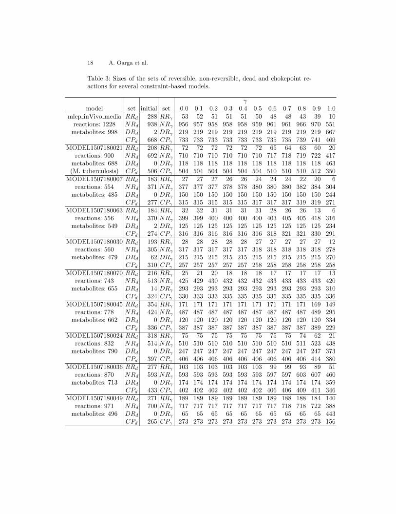
Table 3 reports the sizes of the sets of reversible, non-reversible, dead and choke-point reactions for several constraint-based models of the Biomodels repository[3]. All the results were computed by the tool findCPcli. The maximum CPUtime was 82.776s to compute the results of model MODEL1507180017 in an IntelCore i5-9300H CPU @ 2.40GHz × 8.

18 A. Oarga et al.

Table 3: Sizes of the sets of reversible, non-reversible, dead and chokepoint re-actions for several constraint-based models.

γmodel set initial set 0.0 0.1 0.2 0.3 0.4 0.5 0.6 0.7 0.8 0.9 1.0

mlep inVivo media RRd 288 RRγ 53 52 51 51 51 50 48 48 43 39 10reactions: 1228 NRd 938 NRγ 956 957 958 958 958 959 961 961 966 970 551

metabolites: 998 DRd 2 DRγ 219 219 219 219 219 219 219 219 219 219 667CPd 668 CPγ 733 733 733 733 733 733 735 735 739 741 469

MODEL1507180021 RRd 208 RRγ 72 72 72 72 72 72 65 64 63 60 20reactions: 900 NRd 692 NRγ 710 710 710 710 710 710 717 718 719 722 417

metabolites: 688 DRd 0 DRγ 118 118 118 118 118 118 118 118 118 118 463(M. tuberculosis) CPd 506 CPγ 504 504 504 504 504 504 510 510 510 512 350

MODEL1507180007 RRd 183 RRγ 27 27 27 26 26 24 24 24 22 20 6reactions: 554 NRd 371 NRγ 377 377 377 378 378 380 380 380 382 384 304

metabolites: 485 DRd 0 DRγ 150 150 150 150 150 150 150 150 150 150 244CPd 277 CPγ 315 315 315 315 315 317 317 317 319 319 271

MODEL1507180063 RRd 184 RRγ 32 32 31 31 31 31 28 26 26 13 6reactions: 556 NRd 370 NRγ 399 399 400 400 400 400 403 405 405 418 316

metabolites: 549 DRd 2 DRγ 125 125 125 125 125 125 125 125 125 125 234CPd 274 CPγ 316 316 316 316 316 316 318 321 321 330 291

MODEL1507180030 RRd 193 RRγ 28 28 28 28 28 27 27 27 27 27 12reactions: 560 NRd 305 NRγ 317 317 317 317 317 318 318 318 318 318 278

metabolites: 479 DRd 62 DRγ 215 215 215 215 215 215 215 215 215 215 270CPd 310 CPγ 257 257 257 257 257 258 258 258 258 258 258

MODEL1507180070 RRd 216 RRγ 25 21 20 18 18 18 17 17 17 17 13reactions: 743 NRd 513 NRγ 425 429 430 432 432 432 433 433 433 433 420

metabolites: 655 DRd 14 DRγ 293 293 293 293 293 293 293 293 293 293 310CPd 324 CPγ 330 333 333 335 335 335 335 335 335 335 336

MODEL1507180045 RRd 354 RRγ 171 171 171 171 171 171 171 171 171 169 149reactions: 778 NRd 424 NRγ 487 487 487 487 487 487 487 487 487 489 295

metabolites: 662 DRd 0 DRγ 120 120 120 120 120 120 120 120 120 120 334CPd 336 CPγ 387 387 387 387 387 387 387 387 387 389 229

MODEL1507180024 RRd 318 RRγ 75 75 75 75 75 75 75 75 74 62 21reactions: 832 NRd 514 NRγ 510 510 510 510 510 510 510 510 511 523 438

metabolites: 790 DRd 0 DRγ 247 247 247 247 247 247 247 247 247 247 373CPd 397 CPγ 406 406 406 406 406 406 406 406 406 414 380

MODEL1507180036 RRd 277 RRγ 103 103 103 103 103 103 99 99 93 89 51reactions: 870 NRd 593 NRγ 593 593 593 593 593 593 597 597 603 607 460

metabolites: 713 DRd 0 DRγ 174 174 174 174 174 174 174 174 174 174 359CPd 433 CPγ 402 402 402 402 402 402 406 406 409 411 346

MODEL1507180049 RRd 271 RRγ 189 189 189 189 189 189 189 188 188 184 140reactions: 971 NRd 700 NRγ 717 717 717 717 717 717 717 718 718 722 388

metabolites: 496 DRd 0 DRγ 65 65 65 65 65 65 65 65 65 65 443CPd 265 CPγ 273 273 273 273 273 273 273 273 273 273 156

Growth Dependent Computation of Chokepoints in Metabolic Networks 19

MODEL1507180068 RRd 361 RRγ 84 84 84 84 84 80 80 77 77 77 71reactions: 1056 NRd 695 NRγ 568 568 568 568 568 572 572 575 575 575 463

metabolites: 911 DRd 0 DRγ 404 404 404 404 404 404 404 404 404 404 522CPd 549 CPγ 469 469 469 469 469 471 471 474 474 474 395

MODEL1507180060 RRd 254 RRγ 57 57 57 57 54 54 52 50 50 48 8reactions: 1075 NRd 821 NRγ 610 610 610 610 613 613 615 617 617 619 356

metabolites: 761 DRd 0 DRγ 408 408 408 408 408 408 408 408 408 408 711CPd 441 CPγ 363 363 363 363 364 364 366 368 368 370 304

MODEL1507180020 RRd 256 RRγ 50 48 48 48 47 47 45 45 45 45 12reactions: 1110 NRd 751 NRγ 556 558 558 558 559 559 561 561 561 561 367

metabolites: 879 DRd 103 DRγ 504 504 504 504 504 504 504 504 504 504 731CPd 455 CPγ 396 398 398 398 398 398 400 400 400 400 319

MODEL1507180059 RRd 630 RRγ 203 203 203 203 203 203 202 202 200 196 142reactions: 1112 NRd 482 NRγ 511 511 511 511 511 511 512 512 514 518 358

metabolites: 1101 DRd 0 DRγ 398 398 398 398 398 398 398 398 398 398 612CPd 470 CPγ 436 436 436 436 436 436 436 436 436 438 306

MODEL1507180013 RRd 551 RRγ 249 249 249 249 249 249 249 249 247 242 49reactions: 1245 NRd 694 NRγ 708 708 708 708 708 708 708 708 710 715 390

metabolites: 987 DRd 0 DRγ 288 288 288 288 288 288 288 288 288 288 806CPd 484 CPγ 533 533 533 533 533 533 533 533 534 536 346

MODEL1507180058 RRd 452 RRγ 155 155 155 155 155 155 155 155 150 147 97reactions: 1285 NRd 833 NRγ 904 904 904 904 904 904 904 904 909 912 547

metabolites: 943 DRd 0 DRγ 226 226 226 226 226 226 226 226 226 226 641CPd 584 CPγ 611 611 611 611 611 611 611 611 614 616 409

MODEL1507180015 RRd 1093 RRγ 510 510 510 510 510 510 510 510 510 510 334reactions: 1681 NRd 588 NRγ 822 822 822 822 822 822 822 822 822 822 667

metabolites: 1381 DRd 0 DRγ 349 349 349 349 349 349 349 349 349 349 680CPd 473 CPγ 612 612 612 612 612 612 612 612 612 612 551

MODEL1507180054 RRd 546 RRγ 85 85 85 82 80 80 77 77 75 71 10reactions: 2262 NRd 1716 NRγ 1138 1138 1138 1141 1143 1143 1146 1146 1148 1152 397

metabolites: 1658 DRd 0 DRγ 1039 1039 1039 1039 1039 1039 1039 1039 1039 1039 1855CPd 1039 CPγ 748 748 748 750 750 750 752 752 754 759 319

MODEL1507180017 RRd 606 RRγ 85 85 85 81 80 78 78 77 77 75 13reactions: 2546 NRd 1923 NRγ 1504 1504 1504 1508 1509 1511 1511 1512 1512 1514 525

metabolites: 1802 DRd 17 DRγ 957 957 957 957 957 957 957 957 957 957 2008CPd 1112 CPγ 984 984 984 986 986 988 988 988 988 990 478