Growth and productivity: The role of government debt

Growth and productivity: The role of government debt☆

António Afonso a,b, João Tovar Jalles c,⁎a ISEG/UTL, Technical University of Lisbon, Department of Economics, UECE,Research Unit on Complexity and Economics (UECE is supported by FCT (Fundação para a Ciência e a Tecnologia)), Portugalb European Central Bank, Directorate General Economics, Kaiserstraße 29, D-60311 Frankfurt am Main, Germanyc University of Aberdeen, Business School, Edward Wright Building, Dunbar Street, AB24 3QY, Aberdeen, UK

a r t i c l e i n f o a b s t r a c t

Article history:Received 20 October 2011Received in revised form 18 June 2012Accepted 10 July 2012Available online 14 August 2012

Weuse a panel of 155 countries to assess the links between growth, productivity and governmentdebt. Via growth equations we assess simultaneity, endogeneity, cross-section dependence,nonlinearities, and threshold effects. We find a negative effect of the debt ratio. For the OECD, thehigher the debt maturity the higher the economic growth; financial crisis is detrimental forgrowth; fiscal consolidation promotes growth; and higher debt ratios are beneficial to TFP growth.The growth impact of a 10% increase in the debt ratio is −0.2% (0.1%) respectively for countrieswith debt ratios above (below) 90% (30%), and an endogenous debt ratio threshold of 59% can bederived.

© 2012 Elsevier Inc. All rights reserved.

JEL classification:C23E62H50

Keywords:Government debtCrisesPanel analysis

1. Introduction

The relevance of government debt for economic growth has become crucial, particularly in a context where policy makershave to face increasing fiscal imbalances. In terms of economic theory, at moderate levels of government debt, fiscal policy mayinduce growth, with a typical Keynesian behaviour. However, at high debt levels, the expected future tax increases will reduce thepossible positive effects of government debt, decreasing investment and consumption resulting in less employment and loweroutput growth. Unfortunately, the empirical evidence that is currently available to shed light on the importance of governmentdebt (and related aspects) for growth of productivity is not very conclusive. This paper attempts to fill some gaps and intends toprovide some additional empirical evidence of the effects of government debt (and its maturity structure) on output growth andproductivity for advanced countries (OECD) as well as emerging and developing countries.

We have recently observed a revival in this theme fuelled by the substantial worsening of public finances in many advanced (andother) economies as a result of the 2008/09 financial and economic crisis (one recent contribution is due to Reinhart and Rogoff,

International Review of Economics and Finance 25 (2013) 384–407

☆ We are grateful to Giancarlo Corsetti for useful discussions at the beginning of the project, to participants in an ECB seminar for useful comments. Theresearch was conducted whilst João Tovar Jalles was visiting the ECB whose hospitality was greatly appreciated. The opinions expressed herein are those of theauthors and do not necessarily reflect those of the ECB or the Eurosystem.⁎ Corresponding author.

E-mail addresses: [email protected], [email protected] (A. Afonso), [email protected] (J.T. Jalles).

1059-0560/$ – see front matter © 2012 Elsevier Inc. All rights reserved.http://dx.doi.org/10.1016/j.iref.2012.07.004

Contents lists available at SciVerse ScienceDirect

International Review of Economics and Finance

j ourna l homepage: www.e lsev ie r .com/ locate / i re f

http://dx.doi.org/10.1016/j.iref.2012.07.004

mailto:[email protected]



http://dx.doi.org/10.1016/j.iref.2012.07.004

http://www.sciencedirect.com/science/journal/10590560

2010).1 In response, governments around the world implemented important fiscal stimulus. More than ever it is important tounderstand the effects of government debt on growth, capital accumulation and productivity, particularly when associated withfinancial crisis.2

The linkages between fiscal policy and growth have been the object of several analyses. For instance, Gemmell (2004) hassummarised many existing empirical works dividing it into three generation studies depending on the econometric methodsused. Even though our main purpose is empirical in nature, it is worth referring to some initial theoretical contributions whichserve as the underlying basis for our analysis. In particular, Modigliani (1961) and Diamond (1965) first, and later Saint-Paul(1992), take a theoretical approach based on a neoclassical growth model and suggest that an increase in public debt will alwaysdecrease the growth rate of the economy. Regarding the developments of government debt, Corsetti, Kuester, Meier, and Müller(2010) discuss the importance of the reversal of significant fiscal imbalances, to ensure the curbing of government debt, notablyin a context where monetary policy is limited by a zero lower bound regarding policy interest rates.

With respect to the empirical evidence, most papers have focussed on advanced countries. Authors looking atmixed samples suchas Schclarek (2004) focusing on a panel of 59 developing and 24 advanced countries for the period 1970–2002 conclude that, fordeveloping countries, there is always a negative and significant relation between debt and growth. For advanced countries, he doesnot find any robust evidence, suggesting that higher public debt levels are not necessarily associated with lower GDP growth rates.Checherita and Rother (2010) look at the Euro-area from 1970 to 2010 and find a nonlinear impact of debt on growthwith a turningpoint at about 90–100% of GDP. On the same line, Kumar and Woo (2010) used 38 advanced and emerging countries from 1970 to2007 and also find an inverse relationship between initial debt and subsequent growth, controlling for other determinants of growth.

On the other hand, de la Fuente (1997) using OECD countries between 1965 and 1995 reports evidence of a sizeable negativeexternality effect of government on the level of productivity. In addition, Dar and Amirkhalkhali (2002) for a sample of 19 OECDcountries find that Total Factor Productivity (TFP) growth and productivity of capital are weaker in countries with largergovernment (which can be proxied by the debt-to-GDP ratio).

In this study we use cross-sectional/time series data for a panel of 155 developed and developing countries for the period1970–2008. We do not present or test a comprehensive theory of economic growth. Rather, we are investigating the stability ofcoefficients over time and across countries (and groups of homogeneous economies). In the empirical estimation, the papermakes use of growth equations and growth accounting techniques (to explore different channels of impact) and focus on anumber of econometric issues that can have an important bearing on the results. In particular, we assess such issues assimultaneity, endogeneity, the relevance of nonlinearities, and the importance of outliers.

Therefore, this paper contributes to the literature by assessing the debt–growth nexus with a diversified variety of methods,providing sensitivity and robustness, and, in more specific terms, by addressing the following issues: i) The impact of governmentdebt and its maturity on growth, the existence of nonlinearities and the relevance of debt thresholds. ii) The relevance of financialdevelopment (e.g., banking sector development, stock market development, for which we build several financial developmentproxies) and the impact of financial crises (debt, currency and banking) on the debt–growth relationship. iii) On a growthaccounting perspective, the impact on TFP growth (for that purpose we build a measure of TFP), capital stock accumulation,private and public investment. iv) Differences between country groups (OECD vs. Emerging and Developing).

Our main results can be summarised as follows: i) there is a negative effect of the government debt ratio for the full sample;ii) a quadratic debt term is not statistically significant; iii) for the OECD, the longer the average debt maturity the higher theeconomic growth; iv) financial crisis is detrimental for growth, notably with high debt ratios; v) fiscal consolidation promotesgrowth in a non-Keynesian fashion; vi) for countries with debt ratios above (below) 90% (30%) the growth impact of a 10%increase in the debt ratio is −0.2.% (0.1%); vii) an endogenous debt ratio threshold of 59% can be derived for the full sample;viii) financial development, stock market development, financial efficiency and bond market development positively affectgrowth in the OECD; ix) higher debt ratios are beneficial to TFP growth, the growth of capital stock per worker, and detrimental tothe levels of private and public investment; x) the higher the household's debt burden coupled with higher government debt, thelower the output growth; xi) most results are confirmed even after we address cross-sectional dependence.

The paper is organised as follows. Section 2 describes the analytical and econometric methodology. Section 3 presents the data, inparticular the construction of the TFP and financial developmentmeasures. Section 4 discusses ourmain results. Section 5 concludes.

2. Methodology

2.1. Analytical framework

A neoclassical growth model provides the analytical framework for our analysis, and the underlying basic aggregateproduction function can be written as Y=F(L,K), with Y being the real aggregated output; L, labour force or population; K, capital

1 Also in most countries, large budget deficits have coincided in the past with less efficiency government spending, large bureaucracies and othercounterproductive economic policies. Hence, amongst the factors that determine economic growth, fiscal policies in general are of particular interest and suchfiscal-growth nexus (see Zagler and Durnecker, 2003 for a survey) is particularly important in situations of economic downturns where tax revenues tend to fleerather quickly and the spending side adjusts more slowly, which builds up larger deficits and accrues fiscal sustainability problems. On the latter, a recent paperby Afonso and Jalles (2011a) takes a longer-run perspective of fiscal sustainability, via a systematic analysis of the stationarity properties of first-differenced levelof government debt series and disentangling their components using Structural Time Series Models, between 1880 and 2009 for a set of 19 countries and theyconclude that the solvency condition would be satisfied in mostly all cases, and, therefore, longer-run fiscal sustainability could not be rejected.

2 For instance, Shibata and Tian (2012) examine optimal debt reorganization strategies in the presence of agency problems in times of financial distress.

385A. Afonso, J.T. Jalles / International Review of Economics and Finance 25 (2013) 384–407

(physical and human). This model suggests that poor countries should have a high return to capital and a fast growth in transitionto the steady-state. However, there are several factors that could interfere with this result. The estimating equation that will beused is based upon a standard growth model that relates real growth of per capita GDP to the initial level of income per capita,3

investment-to-GDP ratio (a proxy for physical capital in a standard neoclassical production function), a measure of human capitalor educational attainment, and the population growth rate, which is augmented to include the level of government debt (as ashare of GDP)—and some variants based on government debt maturity.4 This is complemented with some controls, one of whichis a measure of trade openness,5 as commonly found in the growth literature to expand the model beyond a closed-economyform.

Ultimately, our aggregate production function is Y=F(L,K,D) with D being a debt-related variable of interest. Specifically, Dalternatively consists of the total government debt ratio; short-term government debt ratio; long-term government debt ratio;short-term government debt as a share of total government debt. The baseline specification assumes a linear relationshipbetween D and growth:

yit−yit−1 ¼ αit þ β0yio þ β1xjit þ γDit þ ηt þ νi þ εit ; t ¼ 1;…; T; i ¼ 1; ::;N ð1Þ

where yit−yit−1 represents the growth rate of real GDP per capita; yi0 is the initial value of the real GDP per capita6; xjit, j=1,2 isa vector of control variables; Dit is a debt-related variable; ηt and vi correspond to the time effect and the country-specific effect,respectively, and εit is some unobserved zero mean white noise-type column vector satisfying the standard assumptions. α, β0, β1

and γ are unknown parameters to be estimated.The vector x1it (benchmark) comprises population growth, trade openness, gross fixed capital formation (% GDP) and an

education proxy for human capital corresponding to Barro and Lee's (2010) secondary school attainment (in Table 1-1 to ‐3). x1itis enlarged with the debt maturity variable as well as an interaction term (in Table 1-4). Table 1-5 includes as controls x1it andfour interaction terms with financial crisis-related dummies. Table 1-7 includes x2it together with a number of interaction termswith debt threshold levels and geographical dummies. We also use alternatively x2it composed of the initial values of the variablesincluded in x1it (apart from population growth) together with the initial values (at the beginning of each 5-year period) forinflation (CPI-based), initial government size, initial financial depth (or liquid liabilities over GDP), banking crisis dummy andgovernment balance ratio (Table 1-9).

To capture a possible non-linear relationship, we also consider a quadratic term in Eq. (1). Such specification would support, inthis context, a so-called Laffer hypothesis if the coefficient on debt is positive and if the coefficient on debt squared is negative.Furthermore, we access the existence of other non-linear and threshold effects by making use of several dummy (binary-type)variables and interaction terms in our regressions, as it will be explained in the next section.

Finally, taking a growth accounting approach, we compute a measure of TFP and we examine the influence of fiscal variables inaffecting its growth rate, as well as the growth rate of per worker capital stock, and private and public investment levels.

2.2. Econometric approaches

2.2.1. Panel techniquesThe argument for cross-section studies over long time spans has been that less interesting short- to medium-term effects, such

as business cycle effects, are thereby eliminated. However, a number of problems with cross-section studies using long time spansneed to be addressed. The most important of these may be a potentially severe simultaneity problem. The cross-countryregressions are usually based on average values over long time periods. In such cases, e.g., the level of government spending islikely to be influenced by demographics, in particular an increasing share of elderly. At the same time the share of elderly iscorrelated with GDP. Thus, errors in the growth variable will affect GDP, demographics and fiscal variables as a share of GDP,which are then correlated with the error term in the growth regression.

A second problem is that cross-section studies using long observation periods give rise to an endogenous selection ofgovernment spending (tax) policy. For example, countries that raise taxes and experience lower growth during the observationperiod are more likely to change the policy stance afterwards and, for instance, reduce taxes, such as Ireland did during the 1980s.

A third related problem is that cross-section analysis may be inefficient since it discards information on within-countryvariation. Whilst both the simultaneity effect and the use of within-country variation are arguments in favour of panel regressionswith shorter time spans, there are also risks. When the period of observation is short, it is less likely that errors in the growthregression may be correlated with government debt which may, in turn, affect the latter's estimated coefficient.

3 The initial level of income per capita is not only a robust and significant variable for growth (in terms of conditional or beta convergence), but output isgenerally correlated with fiscal variables, in particular, tax revenues and government expenditures.

4 The underlying model has its theoretical underpinnings from Landau's (1983), Kormendi and Meguire's (1985) or Ram's (1986) formulations.5 If open economies are especially exposed to shocks, it may be especially important for the government to facilitate private consumption smoothing via

countercyclical policies (Rodrik, 1998). On the other hand, integrated international financial markets may offer more scope to absorb shocks through risk sharing,suggesting there is less need for governments to step in. For instance, Afonso and Furceri (2008) find that such risk sharing is lower amongst the EU countriesthan in the US states.

6 For regressions using annual data, the lagged value of GDP (yit−1) is used instead.

386 A. Afonso, J.T. Jalles / International Review of Economics and Finance 25 (2013) 384–407

Cross-section methods are simple and easy to interpret but relationships may be artificially created or obscured by unobservedheterogeneity and outliers. The use of panel data can overcome (some of) these problems, and has other advantages. As acompromise we focus mainly on combined cross-section time-series regressions using cumulative 5 year non-overlappingaverages to smooth the effects of short-run fluctuations, even though growth regressions will be first estimated with annual data,therefore making use of the full informational advantage of our (unbalanced) dataset. We run (pooled) Ordinary Least Squares toserve as a benchmark model—as common practice in the literature—despite being aware of all the econometric problemsassociated with this method, as previously discussed. We also run a within estimator, fixed effects, with the inclusion of timedummies that allow for common long-run growth in per capita GDP, which is consistent with common technical progress.

2.2.2. Dealing with outliersA closer inspection of the data—next section—suggests that influential outliers could play an important role in cross-section

analysis. The sample sensitivity of some cross-country empirical studies is well known. Therefore, one advance in this paper overearlier work is the use of two robust estimators, the Method of Moments (MM) and the Least Absolute Deviation (LAD). Theformer fits the efficient high breakdown estimator proposed by Yohai (1987) which on the first stage takes the S estimator

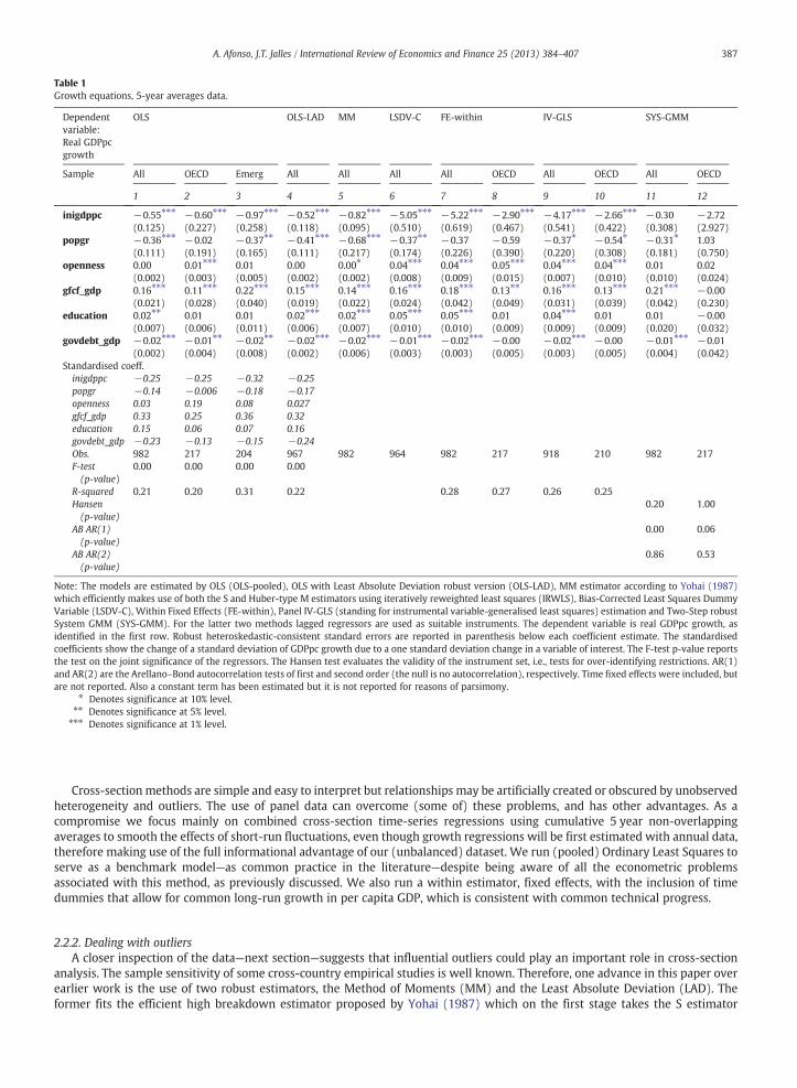
Table 1Growth equations, 5-year averages data.

Dependentvariable:Real GDPpcgrowth

OLS OLS-LAD MM LSDV-C FE-within IV-GLS SYS-GMM

Sample All OECD Emerg All All All All OECD All OECD All OECD

1 2 3 4 5 6 7 8 9 10 11 12

inigdppc −0.55⁎⁎⁎ −0.60⁎⁎⁎ −0.97⁎⁎⁎ −0.52⁎⁎⁎ −0.82⁎⁎⁎ −5.05⁎⁎⁎ −5.22⁎⁎⁎ −2.90⁎⁎⁎ −4.17⁎⁎⁎ −2.66⁎⁎⁎ −0.30 −2.72(0.125) (0.227) (0.258) (0.118) (0.095) (0.510) (0.619) (0.467) (0.541) (0.422) (0.308) (2.927)

popgr −0.36⁎⁎⁎ −0.02 −0.37⁎⁎ −0.41⁎⁎⁎ −0.68⁎⁎⁎ −0.37⁎⁎ −0.37 −0.59 −0.37⁎ −0.54⁎ −0.31⁎ 1.03(0.111) (0.191) (0.165) (0.111) (0.217) (0.174) (0.226) (0.390) (0.220) (0.308) (0.181) (0.750)

openness 0.00 0.01⁎⁎⁎ 0.01 0.00 0.00⁎ 0.04⁎⁎⁎ 0.04⁎⁎⁎ 0.05⁎⁎⁎ 0.04⁎⁎⁎ 0.04⁎⁎⁎ 0.01 0.02(0.002) (0.003) (0.005) (0.002) (0.002) (0.008) (0.009) (0.015) (0.007) (0.010) (0.010) (0.024)

gfcf_gdp 0.16⁎⁎⁎ 0.11⁎⁎⁎ 0.22⁎⁎⁎ 0.15⁎⁎⁎ 0.14⁎⁎⁎ 0.16⁎⁎⁎ 0.18⁎⁎⁎ 0.13⁎⁎ 0.16⁎⁎⁎ 0.13⁎⁎⁎ 0.21⁎⁎⁎ −0.00(0.021) (0.028) (0.040) (0.019) (0.022) (0.024) (0.042) (0.049) (0.031) (0.039) (0.042) (0.230)

education 0.02⁎⁎ 0.01 0.01 0.02⁎⁎⁎ 0.02⁎⁎⁎ 0.05⁎⁎⁎ 0.05⁎⁎⁎ 0.01 0.04⁎⁎⁎ 0.01 0.01 −0.00(0.007) (0.006) (0.011) (0.006) (0.007) (0.010) (0.010) (0.009) (0.009) (0.009) (0.020) (0.032)

govdebt_gdp −0.02⁎⁎⁎ −0.01⁎⁎ −0.02⁎⁎ −0.02⁎⁎⁎ −0.02⁎⁎⁎ −0.01⁎⁎⁎ −0.02⁎⁎⁎ −0.00 −0.02⁎⁎⁎ −0.00 −0.01⁎⁎⁎ −0.01(0.002) (0.004) (0.008) (0.002) (0.006) (0.003) (0.003) (0.005) (0.003) (0.005) (0.004) (0.042)

Standardised coeff.inigdppc −0.25 −0.25 −0.32 −0.25popgr −0.14 −0.006 −0.18 −0.17openness 0.03 0.19 0.08 0.027gfcf_gdp 0.33 0.25 0.36 0.32education 0.15 0.06 0.07 0.16govdebt_gdp −0.23 −0.13 −0.15 −0.24Obs. 982 217 204 967 982 964 982 217 918 210 982 217F-test(p-value)

0.00 0.00 0.00 0.00

R-squared 0.21 0.20 0.31 0.22 0.28 0.27 0.26 0.25Hansen(p-value)

0.20 1.00

AB AR(1)(p-value)

0.00 0.06

AB AR(2)(p-value)

0.86 0.53

Note: The models are estimated by OLS (OLS-pooled), OLS with Least Absolute Deviation robust version (OLS-LAD), MM estimator according to Yohai (1987)which efficiently makes use of both the S and Huber-type M estimators using iteratively reweighted least squares (IRWLS), Bias-Corrected Least Squares DummyVariable (LSDV-C), Within Fixed Effects (FE-within), Panel IV-GLS (standing for instrumental variable-generalised least squares) estimation and Two-Step robustSystem GMM (SYS-GMM). For the latter two methods lagged regressors are used as suitable instruments. The dependent variable is real GDPpc growth, asidentified in the first row. Robust heteroskedastic-consistent standard errors are reported in parenthesis below each coefficient estimate. The standardisedcoefficients show the change of a standard deviation of GDPpc growth due to a one standard deviation change in a variable of interest. The F-test p-value reportsthe test on the joint significance of the regressors. The Hansen test evaluates the validity of the instrument set, i.e., tests for over-identifying restrictions. AR(1)and AR(2) are the Arellano–Bond autocorrelation tests of first and second order (the null is no autocorrelation), respectively. Time fixed effects were included, butare not reported. Also a constant term has been estimated but it is not reported for reasons of parsimony.

⁎ Denotes significance at 10% level.⁎⁎ Denotes significance at 5% level.⁎⁎⁎ Denotes significance at 1% level.


applied to the residual scale and derives starting values for the coefficient vectors, and on the second stage applies the Huber-typebisquare M-estimator using iteratively re-weighted least squares (IRWLS) to obtain the final coefficient estimates.

As for the LAD, it minimises the sum of the absolute deviations. We then exclude any observations for which the LAD residualis more than two standard deviations from the mean residual, before re-estimating the model by OLS or FE. When the two sets ofestimates are very different, then it may be that the observations are drawn from several different regimes, and/or the OLS (FE)estimates are driven by a few outliers. These procedures are not perfect, but should help to exclude the worst outliers, includingsome that would not be identified by more conventional OLS (FE) diagnostics.

2.2.3. EndogeneityOne should address possible endogeneity issues of right-hand side regressors. Whilst country-specific effects might capture

some of the omitted variables (if we miss out an important variable it not only means our model is poorly specified it also impliesthat any estimated parameters are likely to be biased),7 it does not solve the potential problem and one may end up obtainingbiased estimates of the coefficient if the source of heterogeneity is time-varying. Moreover, on the right-hand side of mostestimated equations there is the debt-to-GDP ratio, which is itself a function of real output. It is quite possible that countries withhigher growth potential can support a higher level of government debt. Furthermore, investment is also likely to be endogenousbecause the expectation of high growth usually induces higher investment levels. Therefore, we have re-estimated ourregressions using the bias-corrected least-squares dummy variable (LSDV-C) estimator by Bruno (2005).8

We complement our fixed-effects approach by estimating the main equations using Generalised Methods of Moments (GMM),and to further inspect endogeneity issues we use a panel Instrumental Variable-Generalised Least Squares (IV-GLS) approach.9

We estimate the growth equations by system-GMM (SYS-GMM) which jointly estimates the equations in first differences,using as instruments lagged levels of the dependent and independent variables, and in levels, using as instruments the firstdifferences of the regressors. As far as information on the choice of lagged levels (differences) used as instruments in thedifference (level) equation, as work by Bowsher (2002) and, more recently, Roodman (2009) has indicated, when it comes tomoment conditions (as thus to instruments) more is not always better. The GMM estimators are likely to suffer from “overfittingbias” once the number of instruments approaches (or exceeds) the number of groups/countries (as a simple rule of thumb). In thepresent case, the validity of instruments was examined using Sargan's test of overidentifying restrictions. Intuitively, the systemGMM estimator does not rely exclusively on the first-differenced equations, but exploits also information contained in theoriginal equations in levels.

2.2.4. Cross-sectional dependenceWe are aware of the potential issue (in particular, bias in coefficient estimates) that can arise from a significant cross-sectional

dependence (within similar groups of countries in our sample) in the error term of the model. As put forward by Eberhard,Helmers, and Strauss (2010), the so-called unobserved common factor technique relies on both latent factors in the error termand regressors to take into account the existence of cross-sectional dependence. Developed with the panel-date/time-serieseconometric literature over the course of the past few years, this method has been largely employed in macroeconomic panel dataexercises (see, e.g., Pesaran, 2006; Coakley, Fuertes, and Smith, 2006; Pesaran and Tosetti, 2007; Bai, 2009; Kapetanios, Pesaran,and Takashi, 2009 and Eberhard and Teal, 2011). This common factor methodology takes cross-sectional dependence as theoutcome of unobserved time-varying omitted common variables or shocks which influence each cross-sectional element in adifferent way. Cross-sectional dependence in the error term of the estimated model results then in inconsistent coefficientestimates if independent variables are correlated with the unspecified common variables or shocks.10

With this in mind, we test for the presence of cross-sectional dependence using Pesaran's (2004) CD test statistic. We rely onthe Pesaran (2006) common correlated effects pooled (CCEP) estimator, a generalisation of the fixed effects estimator that allowsfor the possibility of cross section correlation. Including the (weighted) cross sectional averages of the dependent variable andindividual specific regressors is suggested by Pesaran (2006, 2007, 2009) as an effective way to filter out the impacts of commonfactors, which could be common technological shocks or macroeconomic shocks, causing between group error dependence.

3. Building the dataset

We investigate the relationship between government debt and real per capita GDP growth and TFP growth in a sample of 155countries over the 1970–2008 period. The dataset excludes countries with poor data collection, as measurement error is likely tobe large. All variables are in logs with the exception of shares and growth rates.

7 If our variables are uncorrelated with the omitted variables, then results may be unbiased. Thus, if we do not use any predictors that might be correlated withwhat we imagine to be an important omitted variable, we may be able to reduce the bias. That is why we do not wish to have too many variables in our model. Ifwe use a predictor that is correlated with an omitted variable, we generate endogeneity bias. On the other hand, the more variables we consider the less likely it isthat we are omitting something.

8 Kiviet (1995) uses asymptotic expansion techniques to approximate the small sample bias of the standard LSDV estimator for samples where N is small oronly moderately large. Bruno (2005) extends the bias approximation formulas to accommodate unbalanced panels with a strictly exogenous selection rule.

9 Where endogenous variables are instrumented by appropriate lagged levels and tested by looking at first-stage regression estimates, as common practice inthe literature.10 There are different ways to account for such error cross-sectional dependences (see, e.g., Sarafidis and Wansbeek, 2010 for an overview).


The dataset was collected from several sources.11 Real GDP per capita was retrieved from the World Bank's WordDevelopment Indicators (WDI); gross fixed capital formation (as share of GDP) was retrieved from the same source; publicinvestment (as a share of GDP) was also taken from the same source together with AMECO for advanced countries; weconstructed TFP based on data from the latest version 6.3 of the PennWorld Table (PWT) of Heston, Summers, and Aten (2009)—see section below. The debt-to-GDP ratio comes from IMF's debt historical database compiled by Abbas, Belhocine, ElGanainy, andHorton (2010).

With respect to human capital proxies we mainly rely on the average years of schooling of the population over 25 years oldfrom the international data on educational attainment by Barro and Lee (2010), but we also take the literacy rate (% of people ages15 to 24), primary school enrolment (% gross), primary school duration (years), secondary school enrolment (% gross), secondaryschool duration (years), tertiary school enrolment (% gross) and tertiary school duration (years) from the WDI, for robustnesspurposes.

As for other controls and variables most come from either the WDI or the IMF's IFS, as follows: land area (in squarekilometres), population, real interest rate (%), interest rate spread (lending rate minus deposit rate), imports and exports of goodand services (BoP, current USD), labour participation rate (% of total), labour force, unemployment, total (% of total labour force),fertility rate (births per woman), age dependency ratio (% of working age population), urban population (% of total), short-termdebt (% of exports of goods and services), terms of trade adjustment (constant LCU), real effective exchange rate index(2000=100), come from WDI.

3.1. Growth accounting—Total Factor Productivity

In order to assess how fiscal developments may impinge on TFP we construct a new dataset for this variable, for a largenumber of developed and developing countries, in the periods 1960–2007 and 1970–2007, depending on the availability ofinvestment data for the periods 1950–1960 and 1960–1970, respectively. Naturally, the TFP construction based on the latterperiod encompasses a larger number of countries. National income and product account data and labour force data are obtainedfrom the latest version 6.3 of the PennWorld Table (PWT) of Heston et al. (2009). We gathered the following variables: “rgdpwok”(real GDP per worker) and “Ky” (physical capital to output ratio). To construct the labour quality index of human capital (H), wetake average years of schooling in the population over 25 years old from the international data on educational attainment (E) byBarro and Lee (2010). Annual data on years of schooling from 1960 up to 2000 were retrieved from Klenow and Rodriguez-Clare(2005) dataset and then complemented with information up to 2007 using the Barro and Lee (2010) dataset together with linearinterpolation methods. Appendix 1a details the construction of the TFP variable.

3.2. Financial development proxies

We also chose to take a further step into combining different proxies of financial development, which will then be interactedwith the debt variable in our regressions, by using Principal Components Analysis (PCA). The conventional measures of financialdevelopment are based on Ross Levine's database,12 on which the principal component analysis is applied (following Huang's,2010 approach). See Appendix 1b for a detailed description on how we constructed the different financial development proxies:overall financial development, financial intermediary development, stock market development, financial efficiency, financial sizedevelopment and bond market development.

4. Empirical analysis

4.1. Descriptive statistics and graphical analysis

Since we are largely interested in the relationship between growth (and TFP) and debt, it is instructive to aggregate our datainto one big cross-section spanning from 1970 to 2008 and analyse some scatter plots. Fig. 1.a shows per capita real GDP growthagainst the ratio of government debt-to-GDP for the full sample. It seems that a negative relationship between the two variablescan be extracted, attested by a linear fit. Fig. 1.b looks at the OECD only but in this case, no clear relationship is found. Lastly, whentaking the sub-sample consisting of emerging and developing countries—Fig. 1.c—we also find some evidence of a negativerelationship. If one takes a quadratic fit instead (not shown), to account for a possible non-linear behaviour between debt andgrowth, the 95% confidence interval includes slightly more countries.

We find roughly a similar picture (not shown) when plotting the growth rate of TFP against the ratio of government debt-to-GDP for the full sample and emerging and developing sub-sample, that is, a negative relation. However, our graphicalrepresentation suggests a positive relationship between TFP growth and the debt-to-GDP ratio for the OECD sub-sample (Fig. 1.d).In addition, from plotting the Kernel density estimates (now shown) we observe that government debt has increased throughout

11 For a detailed summary table with definitions, acronyms and sources the reader should consult Appendix 2.12 The description of these measures draws on Demirgüç-Kunt and Levine (1996, 1999).


time, which implies an increase of the size of the government notably when trying to provide the additional services related to thewelfare state.13

4.2. Results: government debt

4.2.1. Debt–growth relationshipWe begin our analysis by estimating a growth regression using annual data, for the period 1970–2008, using as regressors the

initial level of GDP, population growth, trade openness, private investment (gross fixed capital formation), education andgovernment debt (our variable of interest). Results (not shown for reasons of parsimony) are in line with the growth literature, aswe find significantly negative coefficients for the initial level of per capita GDP (conditional convergence hypothesis, confirmingthe catching-up process underlying a longer distance to the steady-state) and population growth, and significantly positivecoefficients for trade openness,14 private investment and education levels. We will refrain from commenting on these resultsagain for the remainder of the paper as they are generally consistent and robust throughout. As for the debt-to-GDP ratio evidencepoints to a statistically significant negative relationship with GDP per capita growth rates for the full sample (pooled OLS andoutlier robust estimators).15

It is important to acknowledge that private credit may bear a complementary relationship with government debt, notably inthe context of economic growth. Therefore, we have included an interaction term between a measure of credit issued to theprivate sector by banks and other financial intermediaries (divided by GDP), excluding credit given to the government,government agencies and public enterprises, and government debt-to-GDP ratio. We still obtain statistically significant negativeestimates of the debt-to-GDP ratio on output growth and, additionally, a negative coefficient for the interaction term, meaningthat the higher the household's debt burden coupled with higher government debt, the lower output growth will be (not shown).

13 In Afonso and Jalles (2011b) the authors address how government size affects economic performance by constructing first a theoretical growth model andthen testing the relationship in an empirical section.14 This translates the successive openness process to international trade flows (removal of trade barriers and other sort of protectionism duties) by manycountries, which has been intensified over the last few decades.15 Estimations with outlier-robust techniques don't change qualitatively our main results. The observations excluded are: Angola, Argentina, Azerbaijan, Belize,Chad, Congo (Rep.), Gabon, Iran, Jordan, Kuwait, Lebanon, Malawi, Nicaragua, Nigeria, Oman, Paraguay, Qatar, Sierra Leone, St. Lucia, Swaziland, Syria, Togo,Trinidad and Tobago, UAE, Uruguay, Vanatu, Venezuela and Zimbabwe.

(a)

-2

-4

0

2

4

6

8

10

real

GD

P g

row

th r

ate

(%)

Government Debt-to-GDP (%)

Full Sample (with linear fit)

(b)

0

1

2

3

4

5

6

7

real

GD

P g

row

th r

ate

(%)


OECD (with linear fit)

(d)(c)

-4

-2

0

2

4

6

8

10

real

GD

P g

row

th r

ate

(%)


Emerging and Developing (with linear fit)

-2

0

2

4

6

8

10

0 50 100 150 2000 20 40 60 80 100 120 140

20 40 60 80 100 120 140

0 50 100 150 200

0

TF

P g

row

th r

ate

(%)


OECD (with linear fit)

Fig. 1. Scatter plots of real GDPpc growth and TFP, against the ratio of Government Debt (% of GDP) in different samples.


As a robustness exercise we have also estimated a model excluding the debt-to-GDP ratio, but explicitly including private creditand the interaction term between the two variables. Results (not shown) suggest that private credit by itself has a statisticallypositive effect on growth, however, the interaction term yields statistically negative coefficients for the all sample which arerobust across econometric specifications (OLS, FE and SYS-GMM). The negative coefficient makes not only the effect of the debt-to-GDP ratio conditional on the level of private credit, but vice versa. In fact, it implies that private credit itself boosts growthgiven a low level of the debt-to-GDP ratio. However, the negative coefficient on the interaction term has the interestingimplication that there exists a threshold level of the debt ratio above which private credit can actually dampen growth.

For the remainder of the paper we focus on 5-year averages, as common practice in the literature. Regarding the full samplewe find evidence that an increase in the debt-to-GDP ratio is detrimental to output growth and this is robust across econometricspecifications, as reported in Table 1.

Moreover, for the OECD sub-group, the same conclusion seems to apply when running pooled OLS (and the coefficient is nowsignificant at 5% level). It is instructive to briefly discuss the size of the standardised coefficients—these indicate the relativeimportance of the variables included in the model: a big impact comes from the initial level of per capita GDP as well as from thepopulation growth rate; private investment also accounts for a sizeable share; and the negative impact of the debt-to-GDP ratio isconfirmed (an increase of 10 pp in the debt ratio reduces the growth rate of real per capita GDP by 0.2% per year).

In order to explore nonlinearities we re-run the same model with a quadratic-debt-term included as an additional regressor.Results (not shown) do not provide evidence of any significant quadratic-debt-term. As a robustness exercise, we have includedalso credit to the private sector in our 5-year averages dataset and the same conclusions as for the use of annual data apply. Wehave redone these estimations taking potential GDP growth as an alternative dependent variable.16 In particular, we took thesmoothed or detrended GDP series extracted for each country making use of i) the Hodrick–Prescott, ii) the Baxter–King andiii) the Christiano–Fitzgerald random walk filters. Computing the growth rates of these new series and using them as alternativedependent variables, yield similar results.

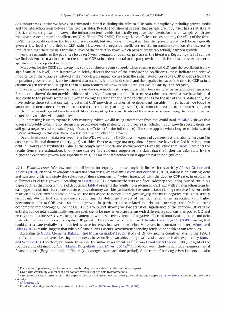
An interesting issue to explore is debt maturity, which we did using information from the World Bank.17 Table 2 shows thatwhen short-debt-to-GDP ratio (defined as public debt with maturity up to 5 years) is included in our growth specifications westill get a negative and statistically significant coefficient (for the full sample). The same applies when long-term debt is usedinstead, although in this case there is a less detrimental effect on growth.

Due to limitations in data retrieved from the WDI, we used the OECD's own measure of average debt to maturity (in years) toconstruct additional dummy (binary type) variables. For the average maturity above 5 years we have classified it as long-termdebt (dumlong) and attributed a value 1; the complement (short- and medium-term) takes the value zero. Table 3 presents theresults from these estimations. In only one case we find evidence supporting the claim that the higher the debt maturity thehigher the economic growth rate (specification 3). As for the interaction term it appears not to be significant.

4.2.1.1. Financial crises. We now turn to a different, but equally important topic. In line with research by Afonso, Gruner, andKolerus (2010) on fiscal developments and financial crises, we take the Laeven and Valencia's (2010) database on banking, debtand currency crisis and study the relevance of these phenomena,18 when interacted with the debt-to-GDP ratio, in explainingdifferences in output growth. According to Easterly (2001), econometric tests and fiscal solvency accounting carried out in hispaper confirm the important role of debt crises. Table 4 presents the results from adding govdebt_gdpwith an interaction term foreach type of crisis introduced one at a time, plus a dummy variable (available in the same dataset) taking the value 1 when a debtrestructuring occurred and zero otherwise. The first aspect to notice is that govdebt_gdp retains its negative and is statisticallysignificant. We do find some evidence supporting the detrimental effect of financial crises when associated with highergovernment debt-to-GDP levels on output growth, in particular those related to debt and currency crises (robust acrosseconometric methodologies). For the OECD sub-group (not shown) we lose statistical significance of the debt-to-GDP variableentirely, but we retain statistically negative coefficients for most interaction terms with different types of crisis (in pooled OLS andFE cases; not in the SYS-GMM though). Moreover, we now have evidence of negative effects of both banking crises and debtrestructuring operations on per capita GDP growth. This seems to be in line with Reinhart and Rogoff's (2009) finding thatbanking crises are typically accompanied by large increases in government debts. Moreover, in a companion paper—Afonso andJalles (2012)—results suggest that when a financial crisis occurs, government spending tends to be stickier than revenues.

According to Gupta, Clements, Baldacci, and Mulas-Granados' (2005) study of 39 low income countries (during the 1990s)initial conditions also have a bearing on the nexus between fiscal variables and growth, and an avenue is also explored by Kumarand Woo (2010). Therefore, we similarly include the initial government size19 (from Gwartney & Lawson, 2006), in light of therobust results obtained by Sala-i-Martin, Doppelhofer, and Miller (2004).20 In addition, we include initial trade openness, initialfinancial depth (llgdp) and initial inflation (all averaged over each time period). A measure of banking crises incidence is also

16 For reasons of parsimony results are not shown but they are available from the authors on request.17 Given data availability a number of observations were lost due to data transformations.18 One related but unaddressed topic in this paper is the role of oil price shocks in sovereign debt financing. A paper by Chow (1998) looked at this issue morecarefully.19 Cf. footnote 10.20 Fiscal sustainability can also be a motivation, in line with Woo (2003) and Huang and Xie (2008).


Table 2Growth equations with short-debt-to-GDP and long-debt-to-GDP ratios, 5-year averages data.

Dependent variable: Real GDPpc growth OLS OLS-LAD MM LSDV-C FE-within IV-GLS SYS-GMM

Sample All

1 2 3 4 5 6 7 8 9 10 11 12 13 14

inigdppc −0.55⁎⁎⁎ −0.85⁎⁎⁎ −0.49⁎⁎⁎ −0.79⁎⁎⁎ −0.81⁎⁎⁎ −1.05⁎⁎⁎ −6.92⁎⁎⁎ −6.94⁎⁎⁎ −6.40⁎⁎⁎ −6.68⁎⁎⁎ −4.22⁎⁎⁎ −4.86⁎⁎⁎ −0.68 −0.72⁎

(0.184) (0.188) (0.178) (0.181) (0.147) (0.148) (0.770) (0.657) (0.778) (0.806) (0.740) (0.765) (0.477) (0.412)popgr −0.38⁎⁎ −0.38⁎⁎ −0.49⁎⁎⁎ −0.51⁎⁎⁎ −1.11⁎⁎⁎ −0.98⁎⁎⁎ −0.48⁎⁎ −0.48⁎⁎ −0.24 −0.37 −0.15 −0.19 −0.15 −0.35

(0.169) (0.159) (0.168) (0.160) (0.169) (0.259) (0.190) (0.214) (0.245) (0.270) (0.168) (0.179) (0.174) (0.243)openness 0.00 0.00 −0.00 −0.00 −0.00 −0.00 0.04⁎⁎⁎ 0.05⁎⁎⁎ 0.04⁎⁎⁎ 0.05⁎⁎⁎ 0.04⁎⁎⁎ 0.04⁎⁎⁎ 0.01 0.03⁎⁎

(0.004) (0.004) (0.003) (0.003) (0.004) (0.004) (0.010) (0.010) (0.011) (0.010) (0.008) (0.009) (0.012) (0.011)gfcf_gdp 0.17⁎⁎⁎ 0.17⁎⁎⁎ 0.17⁎⁎⁎ 0.16⁎⁎⁎ 0.16⁎⁎⁎ 0.17⁎⁎⁎ 0.16⁎⁎⁎ 0.16⁎⁎⁎ 0.21⁎⁎⁎ 0.19⁎⁎⁎ 0.15⁎⁎⁎ 0.14⁎⁎⁎ 0.22⁎⁎⁎ 0.20⁎⁎⁎

(0.026) (0.025) (0.024) (0.023) (0.036) (0.032) (0.028) (0.030) (0.054) (0.050) (0.029) (0.030) (0.045) (0.044)education 0.02⁎⁎ 0.02⁎⁎ 0.02⁎ 0.02⁎⁎ 0.02⁎⁎⁎ 0.03⁎⁎⁎ 0.08⁎⁎⁎ 0.08⁎⁎⁎ 0.07⁎⁎⁎ 0.08⁎⁎⁎ 0.06⁎⁎⁎ 0.07⁎⁎⁎ 0.03 −0.00

(0.009) (0.009) (0.009) (0.009) (0.007) (0.010) (0.017) (0.015) (0.014) (0.015) (0.014) (0.014) (0.023) (0.023)shortgovdebt_gdp −0.04⁎⁎⁎ −0.04⁎⁎ −0.05⁎⁎ −0.00 −0.00 −0.04⁎⁎⁎ −0.05⁎⁎⁎

(0.016) (0.016) (0.018) (0.021) (0.027) (0.013) (0.016)longgovdebt_gdp −0.02⁎⁎⁎ −0.02⁎⁎⁎ −0.02⁎⁎⁎ −0.01⁎⁎⁎ −0.02⁎⁎⁎ −0.01⁎⁎⁎ −0.02⁎⁎⁎

(0.003) (0.003) (0.003) (0.004) (0.006) (0.004) (0.007)Standardised coeff.inigdppc −0.15 −0.24 −0.14 −0.24popgr −0.12 −0.12 −0.16 −0.17openness 0.004 0.03 −0.03 −0.0005gfcf_gdp 0.33 0.34 0.33 0.34education 0.15 0.17 0.14 0.16shortgovdebt_gdp −0.10 −0.09longgovdebt_gdp −0.24 −0.25Obs. 629 594 620 585 629 594 616 585 629 594 529 493 629 594F-test (p-value) 0.00 0.00 0.00 0.00R-squared 0.18 0.23 0.19 0.24 0.28 0.32 0.27 0.29Hansen (p-value) 0.91 0.89AB AR(1) (p-value) 0.00 0.00AB AR(2) (p-value) 0.29 0.57

Note: The models are estimated by OLS (OLS-pooled), OLS with Least Absolute Deviation robust version (OLS-LAD), MM estimator according to Yohai (1987) which efficiently makes use of both the S and Huber-type Mestimators using iteratively reweighted least squares (IRWLS), Bias-Corrected Least Squares Dummy Variable (LSDV-C), Within Fixed Effects (FE-within), Panel IV-GLS estimation and Two-Step robust System GMM (SYS-GMM). For the latter two methods lagged regressors are used as suitable instruments. The dependent variable is real GDPpc growth, as identified in the first row. Robust heteroskedastic-consistent standard errors arereported in parenthesis below each coefficient estimate. The standardised coefficients show the change of a standard deviation of GDPpc growth due to a one standard deviation change in a variable of interest. The F-test p-value reports the test on the joint significance of the regressors. The Hansen test evaluates the validity of the instrument set, i.e., tests for over-identifying restrictions. AR(1) and AR(2) are the Arellano–Bond autocorrelationtests of first and second order (the null is no autocorrelation), respectively. Time fixed effects were included, but are not reported. Also a constant term has been estimated but it is not reported for reasons of parsimony.


392A.A

fonso,J.T.Jalles/InternationalReview

ofEconomics

andFinance

25(2013)

384–407

considered as we have shown it is important determinant. The fiscal deficit is included to take into account the finding that fiscaldeficits are negatively associated with longer-run growth (see, Fisher, 1993 and Baldacci, Clements, and Gupta, 2003). We get thatbanking crises have indeed a negative impact on output growth which is robust across econometric specifications (as attestedbefore).21 The budget balance is positive and statistically significant in four specifications for the OECD sample, which wouldimply that a fiscal consolidation promotes growth in a non-Keynesian fashion in those cases.22 As before, the debt-to-GDP ratioappears with negative and a significant coefficient for the whole sample and mostly insignificant for the OECD sub-group.

As a robustness exercise we have repeated the analysis without initial conditions of the regressors previously included (apartfrom inigdppc)—hence, replaced with variables averaged over each 5-year period, and results didn't change.23

4.2.2. Debt thresholdsHigh levels of government debt may affect the allocation of resources, hence growth and productivity. In this sub-section we

study the effect of different debt-to-GDP ratio thresholds on growth. We followed Table 4's setting and in addition to govdebt_gdp

21 The full set of results is available upon request.22 Afonso (2010) reports related evidence for the EU.23 Another exercise worth while conducting is a sensitivity analysis of the different explanatory variables included in our regressions. We have re-run theestimations without the budget balance (due to possible collinearity with either government debt or government size) and inflation (which proved not to besignificant in the regression with initial conditions; but statistically negative in the first robustness exercise). Such additional findings confirm the negative effectto debt-to-GDP ratio for the full sample and for the OECD (the latter when running SYS-GMM).

Table 3Growth equations with debt average maturity plus dummy interactions, 5-year averages data—OECD sample.

Dependent variable: Real GDPpc growth OLS FE-within IV-GLS SYS-GMM

Sample OECD

1 2 3 4 5 6 7 8

inigdppc −0.81⁎⁎⁎ −0.72⁎⁎ −6.05⁎⁎⁎ −5.93⁎⁎⁎ −4.48⁎⁎ −4.97⁎⁎ −0.63 −0.56(0.304) (0.313) (1.569) (1.934) (2.158) (2.054) (0.887) (0.473)

popgr −0.06 −0.16 −2.78⁎⁎⁎ −2.38⁎⁎⁎ −1.97⁎⁎⁎ −2.01⁎⁎⁎ 0.41 0.52(0.258) (0.279) (0.718) (0.527) (0.745) (0.692) (0.756) (1.731)

openness 0.01⁎⁎ 0.01⁎⁎ 0.09⁎⁎ 0.11⁎⁎ 0.08⁎⁎⁎ 0.09⁎⁎⁎ 0.00 0.01(0.003) (0.003) (0.042) (0.049) (0.029) (0.030) (0.006) (0.008)

gfcf_gdp 0.06 0.06 0.34⁎⁎⁎ 0.43⁎⁎⁎ 0.21 0.35⁎⁎ −0.03 0.01(0.047) (0.045) (0.080) (0.071) (0.146) (0.167) (0.133) (0.131)

education −0.00 −0.00 0.02 0.03⁎ 0.02 0.01 −0.01 0.01(0.008) (0.008) (0.012) (0.014) (0.028) (0.030) (0.011) (0.016)

debtavtermmat 0.01 0.33⁎ −0.02 −0.02(0.057) (0.184) (0.148) (0.164)

govdebt_gdp −0.00 0.02⁎⁎ 0.02⁎⁎⁎ −0.02(0.004) (0.009) (0.007) (0.021)

govdebt_gdp∗dumlong −0.00 −0.00 −0.00 −0.00(0.003) (0.004) (0.003) (0.004)

Standardised coeff.inigdppc −0.35 −0.31popgr −0.01 −0.04openness 0.19 0.17gfcf_gdp 0.15 0.14education −0.04 −0.03debtavtermmat 0.01govdebt_gdp −0.06Obs. 93 93 93 93 66 66 93 93F-test (p-value) 0.00 0.00R-squared 0.24 0.25 0.46 0.44 0.30 0.36Hansen (p-value) 1.00 1.00AB AR(1) (p-value) 0.77 0.99AB AR(2) (p-value) 0.72 0.92

Note: The models are estimated by OLS (OLS-pooled), Within Fixed Effects (FE-within), Panel IV-GLS estimation and Two-Step robust System GMM (SYS-GMM).For the latter method lagged regressors are used as suitable instruments. The dependent variable is real GDPpc growth, as identified in the first row. Robustheteroskedastic-consistent standard errors are reported in parenthesis below each coefficient estimate. The standardised coefficients show the change of astandard deviation of GDPpc growth due to a one standard deviation change in a variable of interest. The F-test p-value reports the test on the joint significance ofthe regressors. The Hansen test evaluates the validity of the instrument set, i.e., tests for over-identifying restrictions. AR(1) and AR(2) are the Arellano–Bondautocorrelation tests of first and second order (the null is no autocorrelation), respectively. Time fixed effects were included, but are not reported. Also a constantterm has been estimated but it is not reported for reasons of parsimony.



Table 4Growth equations with debt and financial crises, 5-year averages data.

Dependent variable: Real GDPpcgrowth

FE (within) IV-GLS SYS-GMM

Sample All

1 2 3 4 5 6 7 8 9 10 11 12 13 14 15

inigdppc −5.22⁎⁎⁎ −5.29⁎⁎⁎ −5.13⁎⁎⁎ −5.28⁎⁎⁎ −5.33⁎⁎⁎ −4.17⁎⁎⁎ −4.08⁎⁎⁎ −3.83⁎⁎⁎ −4.04⁎⁎⁎ −4.11⁎⁎⁎ −0.52 −0.41 −0.54 −0.37 −0.12(0.619) (0.694) (0.722) (0.711) (0.698) (0.541) (0.566) (0.567) (0.559) (0.570) (0.575) (0.474) (0.535) (0.489) (0.625)

popgr −0.37 −0.56⁎⁎ −0.57⁎⁎ −0.57⁎⁎ −0.57⁎⁎ −0.37⁎ −0.54⁎⁎ −0.54⁎⁎ −0.56⁎⁎ −0.56⁎⁎ −0.18 −0.61 −0.69⁎ −0.68 −0.88(0.226) (0.273) (0.278) (0.265) (0.278) (0.220) (0.231) (0.232) (0.220) (0.237) (0.370) (0.438) (0.376) (0.415) (0.549)

openness 0.04⁎⁎⁎ 0.04⁎⁎⁎ 0.04⁎⁎⁎ 0.04⁎⁎⁎ 0.04⁎⁎⁎ 0.04⁎⁎⁎ 0.04⁎⁎⁎ 0.03⁎⁎⁎ 0.04⁎⁎⁎ 0.04⁎⁎⁎ 0.01 −0.01 0.00 −0.01 0.00(0.009) (0.010) (0.011) (0.010) (0.010) (0.007) (0.007) (0.007) (0.007) (0.007) (0.026) (0.015) (0.014) (0.017) (0.018)

gfcf_gdp 0.18⁎⁎⁎ 0.18⁎⁎⁎ 0.18⁎⁎⁎ 0.18⁎⁎⁎ 0.18⁎⁎⁎ 0.16⁎⁎⁎ 0.16⁎⁎⁎ 0.16⁎⁎⁎ 0.16⁎⁎⁎ 0.16⁎⁎⁎ 0.19⁎⁎⁎ 0.25⁎⁎⁎ 0.23⁎⁎⁎ 0.22⁎⁎⁎ 0.23⁎⁎⁎

(0.042) (0.044) (0.044) (0.044) (0.045) (0.031) (0.032) (0.032) (0.032) (0.032) (0.060) (0.049) (0.049) (0.050) (0.055)education 0.05⁎⁎⁎ 0.05⁎⁎⁎ 0.05⁎⁎⁎ 0.04⁎⁎⁎ 0.05⁎⁎⁎ 0.04⁎⁎⁎ 0.03⁎⁎⁎ 0.03⁎⁎⁎ 0.03⁎⁎⁎ 0.03⁎⁎⁎ 0.03 0.02 0.03 0.03 0.00

(0.010) (0.011) (0.011) (0.011) (0.011) (0.009) (0.009) (0.009) (0.009) (0.009) (0.042) (0.033) (0.035) (0.035) (0.044)govdebt_gdp −0.02⁎⁎⁎ −0.01⁎⁎⁎ −0.02⁎⁎⁎ −0.01⁎⁎⁎ −0.02⁎⁎⁎ −0.02⁎⁎⁎ −0.01⁎⁎⁎ −0.01⁎⁎⁎ −0.01⁎⁎ −0.02⁎⁎⁎ −0.01⁎⁎ −0.00 −0.00 −0.00 −0.01⁎⁎⁎

(0.003) (0.004) (0.003) (0.003) (0.004) (0.003) (0.004) (0.003) (0.004) (0.003) (0.004) (0.006) (0.003) (0.004) (0.003)govdebt_gdp∗bankingcrisis −0.01 −0.00 −0.00

(0.004) (0.004) (0.005)govdebt_gdp∗debtcrisis −0.02⁎⁎⁎ −0.02⁎⁎⁎ −0.02⁎⁎⁎

(0.005) (0.005) (0.006)govdebt_gdp∗currencycrisis −0.01⁎⁎⁎ −0.01⁎⁎⁎ −0.01⁎⁎⁎

(0.004) (0.004) (0.003)govdebt_gdp∗debtrestruct −0.00 0.00 0.01⁎

(0.003) (0.003) (0.004)Obs. 982 876 876 876 876 918 826 826 826 826 982 876 876 876 876R-squared 0.28 0.29 0.29 0.30 0.28 0.26 0.26 0.28 0.28 0.26Hansen (p-value) 1.00 1.00 1.00 1.00 1.00AB AR(1) (p-value) 0.00 0.00 0.00 0.00 0.00AB AR(2) (p-value) 1.00 0.82 0.81 0.76 0.78

Note: The models are estimated by Within Fixed Effects (FE-within), Panel IV-GLS estimation and Two-Step robust System GMM (SYS-GMM). For the latter method lagged regressors are used as suitable instruments. Thedependent variable is real GDPpc growth, as identified in the first row. Robust heteroskedastic-consistent standard errors are reported in parenthesis below each coefficient estimate. The Hansen test evaluates the validityof the instrument set, i.e., tests for over-identifying restrictions. AR(1) and AR(2) are the Arellano–Bond autocorrelation tests of first and second order (the null is no autocorrelation), respectively. Time fixed effects wereincluded, but are not reported. Also a constant term has been estimated but it is not reported for reasons of parsimony.


394A.A

fonso,J.T.Jalles/InternationalReview

ofEconomics

andFinance

25(2013)

384–407

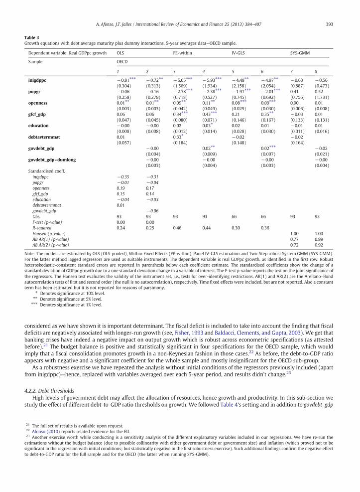
included in each specification, we interacted this variable with a dummy variable (dum30) taking the value 1 if the debt-to-GDPratio was below 30 at a certain point in time, between 60 and 90 (dum3060) or above 90 (dum90), respectively. We find that the30% debt threshold is positive and statistically significant at 1% level in one pooled OLS, one FE, and a SYS-GMM estimation forboth the whole sample, and for the OECD sub-group. The full sample having a debt-to-GDP ratio above 90 affects negativelygrowth.24

In order to have a visual image, we plot the cross-sectional average of per capita GDP growth rates for these levels of debt-to-GDP ratios for the entire sample as well as the OECD and emerging economy sub-groups in Fig. 2. Low debt is defined as havinggovdebt_gdp below 30% and high debt as a level above 90%. A consistent pattern is present, namely countries with low debt ratiosgrow faster (which is also true for the emerging sub-group). No significant difference is found with respect to OECD economies.

We also computed the impact on growth of a given proportional increase in the debt-to-GDP ratio. This was undertaken toallow an appropriate comparison of the impact of government debt on growth at different levels of debt and reflects the fact thatan increase in the ratio from 10 to 20% constitutes a doubling, whilst an increase from 100 to 110% raises it only by one-tenth.Table 5 summarizes the results for debt ratios in three groupings: b30%, 30–60% and >90%. For each of these grouping weobtained the sample average debt ratio (row 1), and then multiplied a given increase (10%) in this ratio, by the estimatedcoefficient of the interaction term (row 2, based on the different estimation techniques). The results (row 3) indicate that thehigher the level of the debt ratio, the higher the negative impact on output growth. For instance, a 10% increase in the debt ratio incountries with debt ratio above 90% is associated with a decline in growth of 0.27%, whilst an identical increase in the debt ratio inthe 30–60% group is associated with a decline in growth around 0.08%.

In Table 6 we run additional regressions with the debt ratio interacted with dummy variables taking the value 1 if the averagedebt ratio of a particular country over that country's time span is above 60 (dumav60), above 70 (dumav70) until we reach thelevel of 100 (dumav100).25 For reasons of parsimony we only report the coefficients of interest and not the full set of estimates.The results show that for the whole sample, irrespective of the threshold level included in the regression, we always find the debt-to-GDP ratio having a negative and statistically significant effect on growth for the pooled OLS and SYS-GMM specifications.Similarly, for emerging countries we have the same result. Nothing can be said with respect to the OECD sub-group.26 Theinteraction terms in specification 1 (for the full sample) suggest that having average debt ratios above 60 further increases theadverse impact of debt on output growth. Indeed, we find interaction terms with statistically significant negative coefficients in8 out of 9 regressions for the full sample.

The effects of non-linearities (and thresholds) are also explored (and confirmed) in the context of budgetary decomposition ofgovernment's revenues and expenditures in Afonso and Jalles (2011c). They explore whether standard regression results(stemming from model selection techniques—EBA and BMA approaches—as well as regression analysis) hold for countries thathave achieved a modicum of macroeconomic (fiscal) stability which is measured in terms of an average level (over either theentire sample period or cross-section) of the budget deficit in percentage of GDP (an ad-hoc number stemming from the EUStability and Growth Pact is chosen and corresponding to a 3% deficit value).

4.2.2.1. Endogenous debt threshold. In the context of defining a plausible debt threshold level, other than specifying it in a purelyad-hoc way, we now explore the endogenous determination of the debt-to-GDP threshold ratio which is the threshold value inthe empirical model that provides the best fit by maximizing its likelihood. Based on a reduced form growth equation allowing forthe presence of multiple equilibria (like in Straubhaar, Suhrcke, & Urban, 2002), we can employ Hansen's (1996, 2000) techniquesto a (generalised) threshold regression of the form:

yit−yit−1 ¼ α01 þ α11yi0 þ α21Xit→if G > γα02 þ α12yi0 þ α22Xit→if Gbγ

ð2Þ

24 Results available upon request.25 A more disaggregated analysis (in 5 percentage intervals) is available upon request.26 If we re-run the estimations without initial conditions (not shown) little changes occur apart from the fact that i) we loose some significant coefficients forspecification 1 (full sample) but ii) we gain some significantly negative coefficients with fixed-effects estimation in specification 4, and, more importantly, theOECD sub-group has a significantly negative coefficient in the debt-to-GDP ratio when govdebt ∗dumav95 is included as an additional regressor.

GDPpc growth

00.5

11.5

22.5

33.5

44.5

5

All-lowdebt

All-highdebt

OECD-lowdebt

OECD-highdebt

Emerg-lowdebt

Emerg-high debt

%

Fig. 2. GDPpc growth rates for low (b30% GDP) and high (>90% GDP) debt ratios.


where αij, i, j=0,1,2 are regression coefficients and γ is a threshold value that splits the sample in two halves. Xit is a vector ofcontrol variables consisting of population growth, openness, education and investment. The main innovation of the empirical partis to estimate γ endogenously and then split the entire sample accordingly (by examining whether a country performed better(over-performer) or worse (under-performer) than its country-specific growth projection). The threshold variable, G, will be thegovernment debt ratio.

Eq. (2) has an econometric correspondence: a threshold regression model. This model estimation procedure involves threesteps: i) estimating the sample split threshold value; ii) testing whether the endogenously determined sample split value issignificant; and iii) performing conventional hypothesis tests.

The endogenously determined sample split is estimated by minimizing mean square errors, i.e.,

γ ¼ argmine qið Þ′e qið Þqi∈Q

ð3Þ

where qi is the value of the threshold variable (government debt) of region i, Q is the set of all different values of qi, γ is theestimated threshold value of qi, and e(qi) is the vector of OLS residuals of the regression (2) if the sample is split in observationslarger or smaller than qi, and each sample half is estimated separately.

The significance of the sample split could be obtained from a conventional structural break test (Chow test). However, Davies(1977) argued that this test is invalid in the present context, because it assumes that the sample split γ is known with certainty,whilst we estimate it endogenously. A Chow test would not take into account the estimation error of γ and the uncertaintywhether the threshold exists under the null hypothesis. Hansen (1996) suggests a Supremum F-, LM- or Wald-test, which has anon-standard distribution dependent on the sample of observations. The critical values can be obtained by a bootstrap.

Estimating Eq. (2) with cross-sectional 5-year averages and with the annual samples (correcting for heteroskedasticity)27

yields an estimated threshold value γ=59.305 and a corresponding Supremum Wald-test of 27.89 whose p-value is 0.079,indicating a significant sample break for the full sample.28

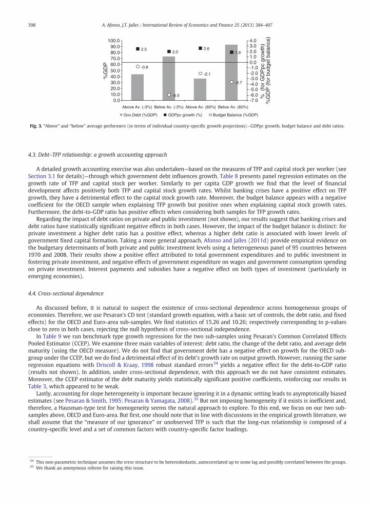
If we take the roughly 60% debt threshold just computed and attempt to summarize GDP growth based on this information wehave in Fig. 3 a visual representation that allows us to draw some meaningful conclusions. In particular, either picking the 60%debt threshold or the 3% budget deficit level, splitting the sample results in having countries with higher debt ratios, and higherbudget deficits, associated with lower growth rates. On the other hand, countries with lower debt ratios and lower fiscalimbalances have higher growth rates.

Regarding the possibility of double threshold effects, and whether other variables may play a role in distinguishing the effectsof fiscal developments on growth that could also be a possibility.29 Nevertheless, we are precisely interested in assessing, whetheror not, high government indebtedness, on its own, undermines economic growth. For instance, somewhat related research hasshowed that the existence of financial crisis further amplifies the negative effects of government spending on growth.30

Interestingly, there is some evidence for some specific economies, using notably Financial Stress Indicators, but not enough dataare available for our panel dataset.31

4.2.2.2. Financial development. One additional issue to keep in mindwhen investigating the relationship between government debtand growth is the level of financial development. The negative impact of government debt on growth could conceivably bestronger in countries with more developed financial systems, translating, for example, a higher private debt stock and associatedburdens (as already partly explored before with the inclusion of private credit).

27 We thank Dieter Urban for kindly making his original code available, which was adapted to our particular needs.28 Using the 5-year averages sample instead, we obtained a statistically significant threshold for the debt-to-GDP ratio of 58.8% (significant Supremum Wald-test of 76.6 with p-value of 0.016). Splitting the sample into OECD countries does not yield a significant debt threshold, but taking the narrower Euro-area sub-sample we find a debt threshold of 58.14% highly significant (at 1% level). Finally, for the emerging countries sub-group a threshold of 79.11% was found for thedebt-to-GDP ratio (significant at 1% level).29 A useful reference on switching regimes is, for instance, Hu and Schiantarelli (1998).30 See Afonso and Jalles (2012).31 See notably Afonso, Baxa, and Slavik (2011) for the cases of the US, the UK, Italy and Germany.

Table 5Impact on real GDP growth per capita of a 10% increase in the debt ratio.

Initial debt ratios (% GDP)

b30 30–60 >90

Sample average of govdebt 14.644 46.542 116.565Regression coefficient, average (1) 0.067 −0.017 −0.023Growth impact of 10% increase in govdebt from sample average (2) 0.098 −0.079 −0.268

Note: (1) average of the estimates (from OLS, FE, SYS-GMM) on the coefficients of interaction terms between initial debt-to-GDP and dummy variables for fourcategories of levels of initial debt-to-GDP (below 30%, between 30 and 60%, between 60 and 90% and above 90% of GDP) for the entire sample period. The resultsare based on coefficients statistically different from zero. However, the statistical significance of the coefficients varies across estimations. (2) This estimate ofgrowth impact of 10% increase in debt ratio is obtained as a product of the regression coefficient (row 2) and 10% of the sample average debt ratios (row 1).


Therefore, we proxy financial development with different measures computed using PCA (see Section 3.2 for details). As a firstexercise, we run a regression including the previous set of initial regressors plus our overall measure of financial development (fd)and the latter interacted with the previously constructed dummies for the debt ratio threshold. In a second exercise, similarly toTable 7, we run independent regressions one at a time with a proxy for financial development and its interaction with the above60% debt threshold, which we have computed as the approximate threshold level.32

The evidence in Table 7 (panel a) suggests that those proxies and the interaction terms are statistically stronger in emergingcountries. Results from the first exercise suggest that overall financial development has a positive effect on growth, but not wheninteracted with debt ratios, and the same is true for the OECD sub-group (according to the fixed-effects estimation). From thesecond exercise (Table 7, panel b), financial development, stock market development, financial size, financial efficiency, and bondmarket development essentially affect positively growth in the OECD sub-group.33 For emerging countries if the debt-to-GDPratio is above 60% both the banking sector development and financial efficiency have a detrimental impact on output growth.

32 Estimating this set of regressions with the outlier-robust MCD version of the newly computed financial development proxies didn't qualitatively change ourmain results.33 Detailed results for fbank, fstock, feff, fsize and fbond are available upon request.

Table 6Growth equation with different levels of Government Debt plus initial regressors, 5 year averages data.

Dependent variable: Real GDPpc growth OLS (pooled) Fixed-Effects (within) SYS-GMM

Sample All OECD Emerg All OECD Emerg All OECD Emerg

1 2 3 4 5 6 7 8 9

Included one at a timegovdebt_gdp −0.02⁎⁎⁎ −0.00 −0.02 −0.01 0.00 0.01 −0.02⁎⁎ −0.02 −0.03⁎

(0.005) (0.006) (0.015) (0.012) (0.010) (0.036) (0.009) (0.020) (0.014)govdebt∗dumav60 −0.01⁎⁎ −0.01 −0.01 −0.01 −0.02 0.03 −0.02⁎ 0.00 −0.03

(0.004) (0.005) (0.010) (0.014) (0.014) (0.056) (0.012) (0.014) (0.023)Obs. 288 129 73 288 129 73R-squared 0.20 0.32 0.53 0.26 0.38 0.38govdebt_gdp −0.02⁎⁎⁎ −0.01 −0.03⁎ −0.01 −0.01 0.01 −0.02⁎ −0.03 0.01

(0.005) (0.008) (0.015) (0.012) (0.013) (0.036) (0.010) (0.029) (0.000)govdebt∗dumav70 −0.01⁎⁎ 0.00 −0.01 −0.01 −0.00 0.03 −0.02 0.02 −0.05

(0.005) (0.006) (0.010) (0.014) (0.013) (0.058) (0.013) (0.029) (0.000)Obs. 288 129 73 288 129 73R-squared 0.20 0.32 0.52 0.26 0.37 0.38govdebt_gdp −0.02⁎⁎⁎ −0.01 −0.03⁎ −0.01 −0.01 0.01 −0.02 −0.03 0.03

(0.005) (0.008) (0.015) (0.011) (0.013) (0.036) (0.012) (0.028) (0.020)govdebt∗dumav80 −0.01⁎⁎ 0.00 −0.01 −0.01 −0.00 0.02 −0.02 0.02 −0.07⁎⁎⁎

(0.005) (0.006) (0.012) (0.015) (0.013) (0.066) (0.013) (0.024) (0.025)Obs. 288 129 73 288 129 73R-squared 0.20 0.32 0.52 0.26 0.37 0.37govdebt_gdp −0.02⁎⁎⁎ −0.01 −0.03⁎ −0.01 −0.01 0.01 −0.02⁎⁎ −0.03 0.03

(0.005) (0.008) (0.015) (0.010) (0.013) (0.036) (0.011) (0.028) (0.020)govdebt∗dumav90 −0.01⁎ 0.00 −0.01 −0.01 −0.00 0.02 −0.01 0.02 −0.07⁎⁎⁎

(0.005) (0.006) (0.012) (0.015) (0.013) (0.066) (0.013) (0.024) (0.025)Obs. 288 129 73 288 129 73R-squared 0.20 0.32 0.52 0.26 0.37 0.37govdebt_gdp −0.01⁎⁎⁎ −0.01 −0.02⁎ −0.00 −0.01 0.04 −0.02⁎ −0.03 −0.03

(0.005) (0.008) (0.013) (0.011) (0.013) (0.038) (0.012) (0.028) (0.031)govdebt∗dumav100 −0.01⁎⁎⁎ 0.00 −0.02 −0.02 −0.00 −0.12⁎⁎⁎ −0.01 0.02 −0.04⁎⁎⁎

(0.005) (0.006) (0.015) (0.013) (0.013) (0.029) (0.012) (0.024) (0.016)Obs. 288 129 73 288 129 73R-squared 0.21 0.32 0.53 0.27 0.37 0.45

Note: The models are estimated by OLS, Within Fixed Effects (FE-within) and Two-Step robust System GMM (SYS-GMM). For the latter method lagged regressorsare used as suitable instruments. The dependent variable is real GDPpc growth, as identified in the first row. For the first panel dumav30, dumav3060 anddumav90, are binary dummy variables taking the value 1 if the average debt-to-GDP ratio of a particular country over the sample's time span is below 30%,between 30 and 60% or above 90%, respectively. For the second panel, we also take the average value of the debt-to-GDP ration for each country as the thresholdlevel, but now dumav60 refers to having that average ratio above 60%. Mutatis mutandis for the remaining levels. Robust heteroskedastic-consistent standarderrors are reported in parenthesis below each coefficient estimate. The Hansen test evaluates the validity of the instrument set, i.e., tests for over-identifyingrestrictions. AR(1) and AR(2) are the Arellano–Bond autocorrelation tests of first and second order (the null is no autocorrelation), respectively. Time fixed effectswere included.



4.3. Debt–TFP relationship: a growth accounting approach

A detailed growth accounting exercise was also undertaken—based on the measures of TFP and capital stock per worker (seeSection 3.1 for details)—through which government debt influences growth. Table 8 presents panel regression estimates on thegrowth rate of TFP and capital stock per worker. Similarly to per capita GDP growth we find that the level of financialdevelopment affects positively both TFP and capital stock growth rates. Whilst banking crises have a positive effect on TFPgrowth, they have a detrimental effect to the capital stock growth rate. Moreover, the budget balance appears with a negativecoefficient for the OECD sample when explaining TFP growth but positive ones when explaining capital stock growth rates.Furthermore, the debt-to-GDP ratio has positive effects when considering both samples for TFP growth rates.

Regarding the impact of debt ratios on private and public investment (not shown), our results suggest that banking crises anddebt ratios have statistically significant negative effects in both cases. However, the impact of the budget balance is distinct: forprivate investment a higher debt ratio has a positive effect, whereas a higher debt ratio is associated with lower levels ofgovernment fixed capital formation. Taking a more general approach, Afonso and Jalles (2011d) provide empirical evidence onthe budgetary determinants of both private and public investment levels using a heterogeneous panel of 95 countries between1970 and 2008. Their results show a positive effect attributed to total government expenditures and to public investment infostering private investment, and negative effects of government expenditure on wages and government consumption spendingon private investment. Interest payments and subsidies have a negative effect on both types of investment (particularly inemerging economies).

4.4. Cross-sectional dependence

As discussed before, it is natural to suspect the existence of cross-sectional dependence across homogeneous groups ofeconomies. Therefore, we use Pesaran's CD test (standard growth equation, with a basic set of controls, the debt ratio, and fixedeffects) for the OECD and Euro-area sub-samples. We find statistics of 15.26 and 10.26; respectively corresponding to p-valuesclose to zero in both cases, rejecting the null hypothesis of cross-sectional independence.

In Table 9 we run benchmark type growth regressions for the two sub-samples using Pesaran's Common Correlated EffectsPooled Estimator (CCEP). We examine three main variables of interest: debt ratio, the change of the debt ratio, and average debtmaturity (using the OECD measure). We do not find that government debt has a negative effect on growth for the OECD sub-group under the CCEP, but we do find a detrimental effect of its debt's growth rate on output growth. However, running the sameregression equations with Driscoll & Kraay, 1998 robust standard errors34 yields a negative effect for the debt-to-GDP ratio(results not shown). In addition, under cross-sectional dependence, with this approach we do not have consistent estimates.Moreover, the CCEP estimator of the debt maturity yields statistically significant positive coefficients, reinforcing our results inTable 3, which appeared to be weak.

Lastly, accounting for slope heterogeneity is important because ignoring it in a dynamic setting leads to asymptotically biasedestimates (see Pesaran & Smith, 1995; Pesaran & Yamagata, 2008).35 But not imposing homogeneity if it exists is inefficient and,therefore, a Hausman-type test for homogeneity seems the natural approach to explore. To this end, we focus on our two sub-samples above, OECD and Euro-area. But first, one should note that in line with discussions in the empirical growth literature, weshall assume that the “measure of our ignorance” or unobserved TFP is such that the long-run relationship is composed of acountry-specific level and a set of common factors with country-specific factor loadings.

34 This non-parametric technique assumes the error structure to be heteroskedastic, autocorrelated up to some lag and possibly correlated between the groups.35 We thank an anonymous referee for raising this issue.

2.52.0

2.61.9

-0.8

-6.0

-2.1

-3.7

0.010.020.030.040.050.060.070.080.090.0

100.0

Above Av. (-3%) Below Av. (-3%) Above Av. (60%) Below Av. (60%)%

GD

P-7.0-6.0-5.0-4.0-3.0-2.0-1.00.01.02.03.04.0

% (

for

GD

Ppc

gro

wth

) %

GD

P (

for

budg

et b

alan

ce)

Gov.Debt (%GDP) GDPpc growth (%) Budget Balance (%GDP)

Fig. 3. “Above” and “below” average performers (in terms of individual country-specific growth projections)—GDPpc growth, budget balance and debt ratios.


We now re-run Table 10's specification 1 (with government debt as our main regressor of interest) using two additionalestimators which allow for parameter and factor loadings heterogeneity/homogeneity. Specifically we rely on the Pesaran andSmith (1995) Mean-Group estimator36 and the factor-loading heterogeneous version, the Pesaran (2006) Common CorrelatedEffects Mean-Group (CCEMG) estimator.37 These estimators are appropriate for the analysis of dynamic panels and they have theadvantage of accommodating both long-run equilibrium and the possibly heterogeneous dynamic adjustment process. TheHausman test will compare estimates from a within fixed-effects estimation with those coming out of the MG and CCEMG,respectively.

Looking at the results displayed in Table 10, we observe that the null hypothesis of slope homogeneity is never rejected atusual significance levels when either the OECD or Euro-area sub-groups are considered (note the associated p-values for a Chi-square statistic with 5 degrees of freedom). This serves as reassurance that our previous estimates are still valid for inferencepurposes.

4.5. “Above” and “below” average performers vis-à-vis fiscal thresholds

To gain additional insight on the relationship between fiscal developments and economic performance, we briefly reviewsome country-specific details related to the regression results reported above (in particular the regression equationcorresponding to specification 1 in Table 2). The main purpose of this exercise is to see if any definite trend can be observedwith respect to government debt and budget deficits and the level of economic performance of the so-called “above-averageperformers” and “below-average performers” (countries), vis-à-vis the fiscal thresholds.

For the full sample we identified above-average and below-average performing countries on the basis of the differencebetween their actual and predicted values of per capita GDP growth rates. In line with Nelson and Singh (1994) countries whoseactual growth rates exceeded their predicted growth rates by 1% or more were classified as “above-average” performers, and

36 The MG approach consists of estimating separate regressions for each country and computing averages of the country-specific coefficients (Evans, 1997; Lee,Pesaran, & Smith, 1997). This allows for heterogeneity of all the parameters.37 Here, the presence of unobserved common factors is achieved by construction and the estimates are obtained as averages of the individual estimates.

Table 7Growth equation with different levels of government debt plus initial regressors and proxies for financial development, 5-year averages data.

Dependent variable: Real GDPpc growth OLS (pooled) Fixed-Effects (within) SYS-GMM

Sample All OECD Emerg All OECD Emerg All OECD Emerg

1 2 3 4 5 6 7 8 9

(Panel a)fd −0.01 0.14 3.29⁎ 1.07 3.30⁎⁎⁎ −4.74⁎⁎ 1.40 −5.56 3.68

(1.068) (1.530) (1.764) (0.773) (1.002) (1.844) (3.199) (7.482) (0.000)fd∗dumav30 −0.87 −0.46 −7.71⁎⁎⁎ −0.72 −2.97⁎⁎⁎ 14.05 −1.34 4.97 6.13

(1.124) (1.633) (1.971) (0.720) (0.963) (12.937) (3.320) (8.699) (0.000)fd∗dumav3060 0.03 −0.00 −5.00⁎⁎ −0.26 −1.98⁎ 2.86 −1.27 5.20 0.79

(1.069) (1.598) (1.827) (0.752) (1.035) (3.397) (3.367) (7.857) (0.000)fd∗dumav90 −0.13 −1.77 −4.13⁎⁎ −0.50 −1.25 2.56 −0.81 7.25 −3.87

(1.387) (2.038) (1.985) (2.049) (2.383) (35.745) (3.205) (9.593) (0.000)Obs. 127 80 36 127 80 36 127 80 36R-squared 0.26 0.26 0.75 0.55 0.70 0.61

Included one at a time (panel b)fd −0.37 −0.07 −2.36⁎⁎⁎ 0.67⁎⁎⁎ 1.00⁎⁎⁎ −0.22 0.03 0.42 0.32

(0.223) (0.285) (0.622) (0.224) (0.362) (2.643) (0.767) (0.900) (2.330)fd∗dumav60 0.26 −0.28 2.61⁎⁎ 0.14 1.48 −3.81 0.13 −1.21 0.09

(0.782) (1.311) (1.038) (0.840) (1.143) (2.564) (1.300) (1.799) (2.739)Obs. 127 80 36 127 80 36 127 80 36R-squared 0.23 0.24 0.66 0.54 0.68 0.60

Note: The models are estimated by OLS, Within Fixed Effects (FE-within) and Two-Step robust System GMM (SYS-GMM). For the latter method lagged regressorsare used as suitable instruments. The dependent variable is real GDPpc growth, as identified in the first row. For the first panel dumav30, dumav3060 anddumav90, are binary dummy variables taking the value 1 if the average debt-to-GDP ratio of a particular country over the sample's time span is below 30%,between 30 and 60% or above 90%, respectively. For the second panel, we also take the average value of the debt-to-GDP ration for each country as the thresholdlevel, but now dumav60 refers to having that average ratio above 60%. Fd, correspond to the first principal component of different financial related variables basedon Levine's publicly available database and it refers to Overall Financial development. For more detailed information do refer to the main text. Robustheteroskedastic-consistent standard errors are reported in parenthesis below each coefficient estimate. The Hansen test evaluates the validity of the instrumentset, i.e., tests for over-identifying restrictions. AR(1) and AR(2) are the Arellano–Bond autocorrelation tests of first and second order (the null is noautocorrelation), respectively. Time fixed effects were included.



countries that fell short of the predicted growth by a similar percentage (or more) were categorized as “below-average”performers. The list of countries in both categories is reported in Table 11. In both cases we run the regression using governmentdebt-to-GDP ratios as the included fiscal variable of interest. The table shows the residual of the per capita GDP growth rate, thegovernment debt ratio, and the budget balance ratio for these groupings of countries.

From examination of the results in Table 11 there is no clear-cut or direct connection between these aggregates. In particular,we cannot conclude that the “above-average” performers (higher residuals in this case) have had necessarily lower debt ratios orbudget deficits and that the “below-average” performers generally experienced larger debts and deficits. For example, we have“below-average” cases (negative residuals) with low levels of government debt and even budget balance surpluses. Conversely inthe “above-average” category we find countries such as Israel with both a high debt ratio and a substantial budget deficit.If one isolates the group of OECD countries (not shown) we also have a mixed picture with, for instance, Greece being in the“above-average” category but with a debt ratio of 62.5% and a budget deficit of 8.1% of GDP. On the other hand, Finland is in the“below-average” category although it has relatively small debt ratio (35.1%) and a budget deficit of 1.1% GDP. Still for OECDcountries, the higher the computed residuals in absolute terms, the lower the debt-to-GDP ratio. The same is true for the budgetbalance in the “above‐average” Performers: the higher the computed residuals, the higher the budget balance (or the lower is thedeficit).

Finally, and in order to summarise the overall effect of government debt on economic growth it is possible to build a densitychart of all the statistically significant estimated coefficients, as depicted in Fig. 4, where the left skewed plot confirms the globalnegative effect of government debt on economic growth.

Table 8Growth accounting with government debt plus initial regressors, 5-year averages data.

Dependentvariable

Growth of TFP Growth of capital stock per worker

Estimation OLS(pooled)

FE(within)

SYS-GMM

OLS(pooled)

FE(within)

SYS-GMM

OLS(pooled)

FE(within)

SYS-GMM

OLS(pooled)

FE(within)

SYS-GMM

Sample All OECD All OECD

1 2 3 4 5 6 7 8 9 10 11 12

lagged dep. var. −0.47⁎⁎⁎ −5.89⁎⁎⁎ −0.71⁎ −3.31⁎⁎⁎ −6.22⁎⁎⁎ −1.57 −0.27⁎⁎⁎ −1.88⁎⁎ −0.15 −0.95⁎⁎⁎ −1.17⁎⁎⁎ 0.20(0.173) (0.727) (0.420) (0.724) (0.971) (0.000) (0.084) (0.706) (0.238) (0.124) (0.295) (1.409)

iniedu −0.01 −0.01 −1.27 1.52⁎ 1.41⁎⁎ −1.15 0.79⁎⁎⁎ 0.17 0.94 −0.27 −0.09 −3.67(0.486) (0.462) (1.439) (0.896) (0.639) (0.000) (0.264) (0.236) (1.015) (0.478) (0.352) (3.554)

iniinf −0.00⁎⁎ −0.00⁎⁎ −0.00 −0.02⁎ 0.00 0.01 0.00 −0.00 0.00 −0.01 −0.01 0.01(0.000) (0.000) (0.003) (0.009) (0.012) (0.000) (0.000) (0.000) (0.001) (0.005) (0.006) (0.032)

inigovsize −0.07 0.16 −0.18 −0.03 −0.01 0.10 −0.07⁎ 0.13 0.01 0.03 0.14 0.07(0.045) (0.106) (0.162) (0.054) (0.151) (0.000) (0.039) (0.092) (0.097) (0.041) (0.083) (0.094)

inifindepth 0.64⁎⁎⁎ 2.62⁎⁎⁎ 2.87⁎⁎⁎ 0.53⁎⁎ 1.03 5.42 0.22⁎ −0.21 0.44 0.21⁎ 0.06 0.43(0.219) (0.703) (1.080) (0.218) (0.615) (0.000) (0.131) (0.453) (0.680) (0.115) (0.358) (0.971)

initrade −0.00 0.00 −0.01⁎ 0.00 −0.00 −0.00 −0.00 0.01 0.01 0.00 0.00 0.00(0.002) (0.006) (0.008) (0.002) (0.005) (0.000) (0.002) (0.007) (0.005) (0.002) (0.004) (0.006)

bankcrisis 0.25 0.29 1.58⁎⁎ −0.06 0.18 −1.47 −0.55⁎⁎⁎ −0.07 −0.20 −0.43⁎⁎ −0.30⁎⁎ −0.43(0.219) (0.182) (0.762) (0.222) (0.142) (0.000) (0.176) (0.167) (0.378) (0.179) (0.122) (0.707)

govbal_gdp −0.01 −0.03 0.07 −0.05⁎⁎ −0.02 −0.08 −0.02 0.05 0.03 0.04⁎⁎⁎ 0.06⁎⁎⁎ 0.06(0.023) (0.024) (0.049) (0.019) (0.021) (0.000) (0.028) (0.031) (0.049) (0.017) (0.019) (0.048)

govdebt_gdp 0.00 0.01⁎⁎ 0.01 −0.00 0.01⁎ −0.03 −0.01⁎⁎⁎ −0.00 −0.00 0.00 0.00 0.00(0.003) (0.003) (0.009) (0.003) (0.004) (0.000) (0.002) (0.004) (0.006) (0.002) (0.004) (0.011)

inigfcf 0.03⁎⁎ −0.03 0.06⁎ −0.05⁎ −0.11⁎⁎ −0.29 0.04⁎⁎⁎ 0.02 0.05 0.04⁎⁎⁎ 0.03 0.06(0.014) (0.020) (0.035) (0.027) (0.042) (0.000) (0.015) (0.023) (0.033) (0.011) (0.023) (0.036)

Obs. 290 290 290 110 110 110 186 186 186 105 105 105R-squared 0.094 0.361 0.372 0.584 0.254 0.381 0.447 0.479Hansen(p-value)

0.709 1.000 0.972 1.000

AB AR(1)(p-value)

0.001 0.075 0.591 0.665

AB AR(2)(p-value)

0.157 0.590 0.163 0.960

Note: The models are estimated by OLS, Within Fixed Effects (FE-within) and Two-Step robust System GMM (SYS-GMM). For the latter method lagged regressorsare used as suitable instruments. The dependent variable is either the growth rate of TFP or the growth rate of the capital stock per worker, as identified in the firstrow. Robust heteroskedastic-consistent standard errors are reported in parenthesis below each coefficient estimate. The Hansen test evaluates the validity of theinstrument set, i.e., tests for over-identifying restrictions. AR(1) and AR(2) are the Arellano–Bond autocorrelation tests of first and second order (the null is noautocorrelation), respectively. Time fixed effects were included, but are not reported. Also a constant term has been estimated but it is not reported for reasons ofparsimony.



5. Conclusion

We have used cross-sectional/time series data for a panel of 155 developed and developing countries for the period 1970–2008, in order to assess the potential linkage between fiscal policy developments and economic growth. More specifically, weused growth equations and growth accounting techniques and focussed also on a number of econometric issues that can have animportant bearing on the results, notably, simultaneity, endogeneity, the relevance of nonlinearities, and threshold effects.

Table 9Growth equations with government debt—accounting for cross-sectional dependence, 5 year averages data—OECD and EURO area.

Dependent variable gdppcgr

Estimation CCEP

Sample OECD EURO OECD EURO OECD EURO

7 8 9 10 11 12

inigdppc −2.90⁎⁎⁎ −1.68 −2.63⁎⁎⁎ −2.42⁎⁎ −6.05⁎⁎⁎ −8.43⁎⁎

(0.543) (1.236) (0.505) (1.069) (1.506) (3.513)popgr −0.59⁎⁎ −1.91⁎⁎⁎ −0.60⁎⁎ −1.78⁎⁎⁎ −2.78⁎⁎⁎ −3.39⁎⁎

(0.280) (0.552) (0.255) (0.460) (0.730) (1.243)gfcf_gdp 0.01 −0.01 0.01 −0.01 0.02 0.02

(0.010) (0.019) (0.010) (0.015) (0.021) (0.043)secondary_enrol 0.13⁎⁎⁎ 0.29⁎⁎⁎ 0.10⁎⁎⁎ 0.15⁎⁎ 0.34⁎⁎⁎ 0.40⁎⁎

(0.042) (0.079) (0.037) (0.069) (0.076) (0.153)openness 0.05⁎⁎⁎ 0.04⁎⁎⁎ 0.03⁎⁎⁎ 0.04⁎⁎⁎ 0.09⁎⁎⁎ 0.12⁎⁎⁎

(0.008) (0.012) (0.008) (0.011) (0.019) (0.035)govdebt_gdp −0.00 0.01

(0.006) (0.011)d.govdebt_gdp −0.02⁎⁎⁎ −0.04⁎⁎⁎

(0.008) (0.012)debtavtermmat 0.33⁎⁎ 0.46⁎

(0.150) (0.258)Obs. 217 109 210 105 93 45R-squared 0.27 0.40 0.28 0.48 0.46 0.49

Note: The models are estimated with the Pesaran's Common Correlated Effects Pooled estimator (CCPE) to correct for the existence of cross-sectional dependencein the OECD and Euro-area groups of countries. The dependent variable is real GDPpc growth, as identified in the first row. Standard errors are reported inparenthesis below each coefficient estimate. A constant term has been estimated but it is not reported for reasons of parsimony.


Table 10Growth equations with government debt—testing slope homogeneity, annual data—OECD and EURO area.

Dependent variable gdppcgr

Estimation MG CCEMG

Sample OECD EURO OECD EURO

1 2 3 4

popgr −2.12⁎ 0.05 −4.76⁎⁎ −3.17⁎⁎⁎

(1.291) (2.566) (2.181) (0.781)gfcf_gdp 0.19 0.12 0.50 0.07

(0.151) (0.129) (0.404) (0.354)secondary_enrol −0.03 −0.05 −0.05 −0.06

(0.057) (0.058) (0.136) (0.101)openness 0.08⁎⁎ 0.08⁎ 0.03 0.08⁎

(0.040) (0.047) (0.082) (0.045)govdebt_gdp −0.03 −0.08 −0.21 −0.21

(0.100) (0.210) (0.334) (0.156)Obs. 439 204 439 204RMSE 1.347 1.005 0.384 0.352Hausman (p-value) 0.84 0.15 0.25 0.26

Note: The models are estimated with either MG or CCEMG estimator in the OECD and Euro-area groups of countries. The dependent variable is real GDPpc growth,as identified in the first row. Standard errors are reported in parenthesis below each coefficient estimate. The Hausman statistic tests the null hypothesis of slopehomogeneity. RMSE stands for Root Mean Square Error. A constant term has been estimated but it is not reported for reasons of parsimony.



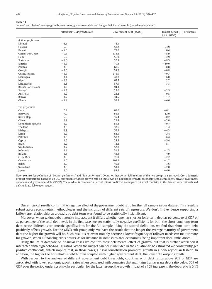
Our empirical results confirm the negative effect of the government debt ratio for the full sample in our dataset. This result isrobust across econometric methodologies and the inclusion of different sets of regressors. We don't find evidence supporting aLaffer-type relationship, as a quadratic debt term was found to be statistically insignificant.

Moreover, when taking debt maturity into account it differs whether one has short or long-term debt as percentage of GDP oras percentage of the total debt level. In the first case, we get statistically negative coefficients for both the short- and long-termdebt across different econometric specifications for the full sample. Using the second definition, we find that short-term debtpositively affects growth. For the OECD sub-group only, we have the result that the longer the average maturity of governmentdebt the higher the growth will be. Such result is relevant notably because a lower frequency of rollover needs can matter morefor growth, when a financing crisis occurs, as for instance in some euro area economies facing important fiscal imbalances.

Using the IMF's database on financial crises we confirm their detrimental effect of growth, but that is further worsened ifinteracted with high debt-to-GDP ratios. When the budget balance is included in the equation to be estimated we consistently getpositive coefficients, which implies that, in those cases, a fiscal consolidation promotes growth in a non-Keynesian fashion. Inaddition, the higher the household's debt burden coupled with higher government debt, the lower the output growth.

With respect to the analysis of different government debt thresholds, countries with debt ratios above 90% of GDP areassociated with lower economic growth rates when compared with countries that maintained an average debt ratio below 30% ofGDP over the period under scrutiny. In particular, for the latter group, the growth impact of a 10% increase in the debt ratio is 0.1%

Table 11“Above” and “below” average growth performers, government debt and budget deficits: all sample (debt-based equation).

“Residual” GDP growth rate Government debt (%GDP) Budget deficit (−) or surplus(+) (%GDP)

Bottom performersKiribati −5.1 16.1Guyana −2.9 58.2 −23.9Kuwait −2.6 72.0 0.4Congo, Dem. Rep. −2.3 138.6 −5.9Haiti −2.2 56.9 −2.9Suriname −2.0 20.9 −8.3Jamaica −1.6 70.8 −10.0Zambia −1.6 60.6 −8.8Georgia −1.6 38.2 −0.8Guinea-Bissau −1.6 216.0 −0.3Nicaragua −1.4 48.7 −6.8Niger −1.3 65.5 2.7Madagascar −1.3 87.9 −3.3Brunei Darussalam −1.3 94.3Senegal −1.3 25.0 −2.5Australia −1.2 24.2 −0.8Bolivia −1.2 34.5 −1.7Ghana −1.1 55.5 −4.6

Top performersOman 5.1 65.0 −6.1Botswana 4.0 56.5 12.0Korea, Rep. 2.9 35.4 −0.2China 2.8 27.4 −2.0Dominican Republic 1.9 51.3 −0.7Thailand 1.8 37.6 −1.4Malaysia 1.8 59.9 −4.3Malta 1.7 63.1 −2.4Pakistan 1.6 58.7 −6.4Cyprus 1.6 24.3 −5.4Israel 1.2 72.8 −8.1Saudi Arabia 1.2 52.8Indonesia 1.1 31.2 −1.3Ireland 1.1 43.5 −4.9Costa Rica 1.0 76.8 −2.2Guatemala 1.0 103.2 −1.7Belize 1.0 49.5 −3.6Swaziland 1.0 53.8 −2.8Japan 1.0 88.5 −4.0

Note: see text for definition of “Bottom performers” and “Top performers”. Countries that do not fall in either of the two groups are excluded. Gross domesticproduct residuals are based on an OLS regression of GDPpc growth rate on initial GDPpc, population growth, secondary school enrolment, private investment,openness and government debt (%GDP). The residual is computed as actual minus predicted. A complete list of all countries in the dataset with residuals anddeficits is available upon request.


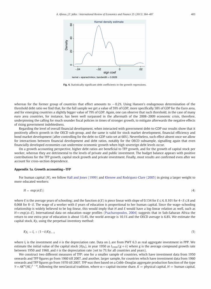
whereas for the former group of countries that effect amounts to −0.2%. Using Hansen's endogenous determination of thethreshold debt ratio we find that, for the full sample we get a value of 59% of GDP, more specifically 58% of GDP for the Euro area,and for emerging countries a slightly bigger value of 79% of GDP. Again, one can observe that such threshold, in the case of manyeuro area countries, for instance, has been well surpassed in the aftermath of the 2008–2009 economic crisis, therefore,underpinning the calling for much sounder fiscal policies in times of stronger growth, to mitigate afterwards the negative effectsof rising government indebtedness.

Regarding the level of overall financial development, when interacted with government debt-to-GDP our results show that itpositively affects growth in the OECD sub-group, and the same is valid for stock market development, financial efficiency andbond market development (after controlling for the debt-to-GDP ratio set at 60%). Nevertheless, such effect absent once we allowfor interactions between financial development and debt ratios, notably for the OECD subsample, signalling again that evenfinancially developed economies can undermine economic growth when high sovereign debt levels occur.

On a growth accounting perspective, higher debt ratios are beneficial to TFP growth, and for the growth of capital stock perworker, whereas they are detrimental to the levels of private and public investment. The budget balance appears with positivecontributions for the TFP growth, capital stock growth and private investment. Finally, most results are confirmed even after weaccount for cross-section dependence.

Appendix 1a. Growth accounting—TFP

For human capital (H), we follow Hall and Jones (1999) and Klenow and Rodriguez-Clare (2005) in giving a larger weight tomore educated workers:

H ¼ exp ϕ Eð Þð Þ ð4Þ

where E is the average years of schooling; and the function ϕ(E) is piece linear with slope of 0.134 for E≤4, 0.101 for 4bE≤8 and0.068 for 8bE. The wage of a worker with E years of education is proportional to her human capital. Since the wage–schoolingrelationship is widely believed to be log-linear, this would imply that H and E would have a log-linear relation as well, such asH=exp(ϕ∗E). International data on education–wage profiles (Psacharopoulos, 2004) suggests that in Sub-Saharan Africa thereturn to one extra year of education is about 13.4%, the world average is 10.1% and the OECD average is 6.8%. We estimate thecapital stock, Ky, using the perpetual inventory method:

Kyt ¼ It þ 1−δð ÞKyt−1 ð5Þ

where It is the investment and δ is the depreciation rate. Data on It are from PWT 6.3 as real aggregate investment in PPP. Weestimate the initial value of the capital stock (Ky0), in year 1950 as I1950/(g+δ) where g is the average compound growth ratebetween 1950 and 1960, and δ is the depreciation rate (set to 7% for all countries and years).

We construct two different measures of TFP: one for a smaller sample of countries, which have investment data from 1950onwards and TFP figures go from 1960 till 2007, and another, larger sample, for countries which have investment data from 1960onwards and TFP figures go from 1970 till 2007. TFP was then based on a Cobb–Douglas aggregate production function of the typeY=AKα(HL)1−α, following the neoclassical tradition, where α=capital-income share, K = physical capital, H = human capital,

020

4060

Den

sity

-.04 -.02 0 .02sign coef

kernel = epanechnikov, bandwidth = 0.0028

Kernel density estimate

Fig. 4. Statistically significant debt coefficients in the growth regressions.


L= labour input and A= TFP. After some mathematical manipulations (dividing both sides by L, taking logs and time derivativesand rearranging) TFP is computed according to the equation below (with a capital-income share α=1/3)38:

TFPit ¼ rgdpwokit= Kyit � rgdpwokitð Þα : exp φ � Hitð Þ 1−αð Þh i: ð6Þ

Appendix 1b. Financial development proxies

The first measure, Liquid Liabilities (llgdp), is calculated as the liquid liabilities of banks and non-bank financial intermediaries(currency plus demand and interest-bearing liabilities) over GDP. The second indicator, Private Credit (pcrdbofgdp), measuresgeneral financial intermediary activities provided to the private sector. The third one, Commercial-Central Bank (dbacba), proxiesthe advantage of financial intermediaries in channelling savings to investment, monitoring firms, influencing corporategovernance and undertaking risk management relative to the central bank.

Efficiency measures for the banking sector: Overhead Costs (overhead), the ratio of overhead costs to total bank assets; and theNet Interest Margin (netintmargin), the difference between bank interest income and interest expenses, divided by total assets.39

Indices for stock market development: Stock Market Capitalization (stmktcap), the size index, is the ratio of the value of listeddomestic shares to GDP. Total Value Traded (stvaltraded), the ratio of the value of domestic shares traded on domestic exchangesto GDP, can be used to gauge market liquidity on an economy-wide basis. Turnover Ratio (stturnover) is the ratio of the value ofdomestic share transactions on domestic exchanges to total value of listed domestic shares.40 Finally, we consider two bondmarket capitalization measures as ratios to GDP, private (prbond) and public (pubond).

Following Huang (2010), we combine the above financial measures as follows: 1) Overall financial development, 1st principalcomponent of pcrdbofgdp, llgdp, dbacba, overhead, netintmargin, stmktcap, stvaltraded and stturnover; 2) Financial intermediarydevelopment, 1st principal component of pcrdbofgdp, llgdp and dbacba; 3) Stock market development, 1st principal component ofstmktcap stvaltraded and stturnover; 4) Financial efficiency development, 1st principal component of overhead, netintmargin,stvaltraded and stturnover; 5) Financial size development, 1st principal component of llgdp and stmktcap; 6) Bond marketdevelopment, 1st principal component of prbond and pubond.

The 1st principal component is normalized in such a way that high values indicate higher financial development. The firststandardised index, overall Financial Development, can be written as41:

f d ¼ 0:67 � pcrdbof gdpþ 0:45 � llgdpþ 0:28 � dbacba−0:16 � overhead−0:25 � netintmarginþ0:81 � stmktcapþ 0:84 � stvaltradedþ 0:33 � stturnover:

In addition, the 1st principal component explains 79% of the total variance in the standardised data. Nevertheless, given ouroutlier discussion and the fact that PCA is based on the classical covariance matrix, which is sensitive to outliers, we take onefurther step. This drawback is easily solved by basing the PCA on a robust estimation of the covariance (correlation) matrix. A wellsuited method is the Minimum Covariance Determinant (MCD) that considers all subsets containing h% of the observations(generally 50%) and estimates ∑ (the variance) and μ (the mean) on the data of the subset associated with the smallestcovariance matrix determinant. We implement Rousseeuw and Van Driessen's (1999) algorithm to estimate new measures forthe previously created aggregated proxies. After re-computing the same measures with the MCD version we obtain similarresults. Moreover, the pair wise correlation coefficients between the 12 different proxies range from 77 to 93% (statisticallysignificant at 1%).

1/ World Bank's Word Development Indicators (WDI). 2/ WDI, 3/ AMECO. 4/ Version 6.3 of the Penn World Table (PWT) ofHeston et al. (2009). 5/ WDI, IMF IFS, Easterly (2001). 6/ IMF (Abbas et al., 2010). 7/ Barro and Lee (2010). 8/ Ross Levine'spublicly available database. 9/Laeven and Valencia (2010).

38 Since consistent data of factor income shares are difficult to obtain for individual countries, most empirical papers assume that income shares are identicalacross time and space. Gollin (2002) provides strong evidence supporting this assumption, which is also consistent with the Cobb–Douglas function approach.Moreover, Bernanke and Gürkaynak (2001) find no systematic tendency for labour shares to vary with real GDP per capita or the capital–labour ratio nor asystematic tendency to rise or fall over time, and most estimated labour income shares lie between 0.6 and 0.8. For our own purposes we take it to be equal to 2/3.39 Lower overhead costs and net interest margins frequently indicate greater competition and efficiency.40 A high value of the turnover ratio indicates a more liquid (and potentially more efficient) equity market.41 A likelihood ratio test was used to examine the “sphericity” case, allowing for sampling variability in the correlations. This test comfortably rejects sphericityat the 1% level with a Kaiser–Meyer–Olkin measure of sampling adequacy equal to 0.753.


Variable Definition/description Acronym

Real GDP per capita gdppc 1/Gross fixed capital formation (% GDP) gfcf_gdp 2/Public investment (% GDP) pubinv_gdp 2/3/Total Factor Productivity Variable constructed using growth accounting

techniquestfp 4/

Government budget surplus or deficit (% of GDP) The government budget surplus or deficit asa percentage of GDP.

govbal_gdp 5/

Central Government Debt (% GDP) govdebt_gdp 6/School attainment Average years of schooling in the population

over 25 years old from the international dataon educational attainment

edu 7/

Literacy rate (% of people ages 15 to 24) literates 2/Primary school enrolment (% gross) primary_enrol 2/Primary school duration (years) primary_dur 2/Secondary school enrolment (% gross) secondaru_enrol 2/Secondary school duration (years) secondary_dur 2/Tertiary school enrolment (% gross) tertiary_enrol 2/Tertiary school duration (years) tertiary_dur 2/Land area (in square kilometres) land_area 2/Population pop 2/Imports and exports of good and services(BoP, current USD)

Imp, exp 2/

Labour participation rate (% of total) Lfp 2/Labour force laborf 2/Unemployment, total (% of total labour force) unemp 2/Fertility rate (births per woman) fertility 2/Age dependency ratio (% of working age population) depratio_wa 2/Urban population (% of total) urban_pop 2/Short-term debt (% of exports of goods and services) short_debt_gdp 2/Terms of trade adjustment (constant LCU) terms_trade 2/Real effective exchange Rate index (2000=100) Reer 2/Liquid Liabilities One of the major indicators to measure the

size, relative to the economy, of financial intermediaries,including three types of financial institutions: the centralbank, deposit money banks and other financial institutions.It is calculated as the liquid liabilities of banks and non-bankfinancial intermediaries (currency plus demand andinterest-bearing liabilities) over GDP.

llgdp 8/

Private Credit Is defined as the credit issued to the private sector by banksand other financial intermediaries divided by GDP excludingcredit issued to government, government agencies and publicenterprises, as well as the credit issued by the monetary authorityand development banks. It measures general financialintermediary activities provided to the private sector.

pcrdbofgdp 8/

Commercial-Central Bank Is the ratio of commercial bank assets to the sum of commercialbank and central bank assets. It proxies the advantage of financialintermediaries in channelling savings to investment, monitoringfirms, influencing corporate governance and undertaking riskmanagement relative to the central bank.

dbacba 8/

Overhead Costs Is the ratio of overhead costs to total bank assets. overhead 8/Net Interest Margin Equals the difference between bank interest income

and interest expenses, divided by total assets. A lowervalue of overhead costs and net interest margin is frequentlyinterpreted as indicating greater competition and efficiency.

netintmargin 8/

Stock Market Capitalization The size index, is the ratio of the value of listed domesticshares to GDP.

stmktcap 8/

Total Value Traded As an indicator to measure market activity, is the ratio of thevalue of domestic shares traded on domestic exchanges toGDP, and can be used to gauge market liquidity on aneconomy-wide basis.

stvaltraded 8/

Turnover Ratio Is the ratio of the value of domestic share transactions ondomestic exchanges to total value of listed domestic shares.A high value of the turnover ratio will indicate a more liquid(and potentially more efficient) equity market.

stturnover 8/

Private bond market capitalization prbond 8/Public bond market capitalization pubond 8/Banking crisis Dummy variable taking the value 1 if a banking crisis occurred

and zero otherwisebankcrisis 9/

Appendix 2. Variables and sources


References

Abbas, A., Belhocine, N., ElGanainy, A., & Horton, M. (2010). A historical public debt database. IMF Working Paper No. 10/245.Afonso, A. (2010). Expansionary fiscal consolidations in Europe: New evidence. Applied Economics Letters, 17(2), 105–109.Afonso, A., Baxa, J., & Slavik, M. (2011). Fiscal developments and financial stress: A threshold VAR analysis. European Central Bank WP 1319.Afonso, A., & Furceri, D. (2008). EMU enlargement, stabilisation costs and insurance mechanisms. Journal of International Money and Finance, 27(2), 169–187.Afonso, A., Gruner, H., & Kolerus, C. (2010). Fiscal policy and growth — Do financial crises make a difference. European Central Bank WP 1217.Afonso, A., & Jalles, J. T. (2011a). A longer-run perspective on fiscal sustainability. ISEG/UTL-Technical University of Lisbon, Department of Economics Working Paper

No. 17/2011/DE/UECE.Afonso, A., & Jalles, J. T. (2011b). Economic performance and government size: A political economy assessment. European Central Bank WP 1399.Afonso, A., & Jalles, J. T. (2011c). Linking investment and fiscal policies. ISEG/UTL-Technical University of Lisbon, Department of Economics Working Paper No. 16/2011/DE/UECE.Afonso, A., & Jalles, J. T. (2011d). Linking investment and fiscal policies. ISEG/UTL-Technical University of Lisbon, Department of Economics, Working Paper

No. 16/2011/DE/UECE.Afonso, A., & Jalles, J. T. (2012). Fiscal volatility, financial crises and growth. Applied Economics Letters, 19(18), 1821–1826.Bai, J. (2009). Panel data models with interactive fixed effects. Econometrica, 77(4), 1229–1279.Baldacci, E., Clements, B., & Gupta, S. (2003, December). Using Fiscal Policy to Spur Growth. Finance and Development, 40, 28–31.Barro, R., & Lee, J. W. (2010). International data on educational attainment, updates and implications. WP 42, Center for International Development, Harvard University.Bernanke, B., & Gürkaynak, R. (2001). Is growth exogenous? Taking Mankiw, Romer, and Weil Seriously. : NBER Working Paper No. 8365.Bowsher, C. G. (2002). On testing overidentifying restrictions in dynamic panel data models. Economics Letters, 77(2), 211–220.Bruno, G. (2005). Approximating the bias of the LSDV estimator for dynamic unbalanced panel data models. Economics Letters, 87(3), 361–366.Checherita, C., & Rother, P. (2010). The impact of high and growing government debt on economic growth— An empirical investigation for the euro area. ECBWorking

Paper No. 1237.Chow, E. (1998). Oil crises and sovereign debt's private financing. International Review of Economics and Finance, 7(4), 437–452.Coakley, Jerry, Fuertes, Ana-Maria, & Smith, Ron (2006). Unobserved heterogeneity in panel time series models. Computational Statistics & Data Analysis, 50(9), 2361–2380.Corsetti, G., Kuester, K., Meier, A., & Müller, G. (2010). Debt consolidation and fiscal stabilization of deep recessions. The American Economic Review, 100(2), 41–45.Dar, A., & Amirkhalkhali, S. (2002). Government size, factor accumulation and economic growth: Evidence from OECD countries. Journal of Policy Modelling, 24, 679–692.Davies, R. B. (1977). Hypothesis testing when a nuisance parameter is only present under the alternative. Biometrika, 64, 247–254.de la Fuente, A. (1997). Fiscal policy and growth in the OECD. CEPR WP, No 1755.Demirgüç-Kunt, A., & Levine, R. (1996). Stock markets, corporate finance and economic growth: An overview. World Bank Economic Review, 10(2), 223–240.Demirgüç-Kunt, A., & Levine, R. (1999). Bank-based and market based financial systems: Cross-country comparisons. World Bank Policy Research working paper no. 2143.Diamond, P. (1965). National debt in a neoclassical growth model. American Economic Review, 55, 1125–1150.Driscoll, John, & Kraay, Aart C. (1998). Consistent covariance matrix estimation with spatially dependent panel data. The Review of Economics and Statistics, 80(4), 549–560.Easterly, W. R. (2001). The lost decades: Developing countries stagnation in spite of policy reform 1980–1998. Journal of Economic Growth, 6(2), 135–157.Eberhard, M., Helmers, C., & Strauss, H. (2010). Do spillovers matter when estimating private returns to R&D? Economic and Financial Reports 2010/1, EIB.Eberhard, M., & Teal, F. (2011). Econometrics for Grunblers: A new look at the literature on cross-country growth empirics. Journal of Economic Surveys, 25(1), 109–155.Evans, P. (1997). How fast do economies converge. The Review of Economics and Statistics, 46, 1251–1271.Fisher, S. (1993). The role of macroeconomic factors in growth. Journal of Monetary Economics, 32(3), 485–512.Gemmell, N. (2004). Fiscal policy in a growth framework. In T. Addison, & A. Roe (Eds.), Fiscal policy for development: Poverty, reconstruction and growth

(pp. 149–176). Great Britain: Palgrave Macmillan.Gollin, D. (2002). Getting income shares right. Journal of Political Economy, 110(2), 458–474.Gupta, S., Clements, B., Baldacci, E., & Mulas-Granados, C. (2005). Fiscal policy, expenditure composition, and growth in low-income countries. Journal of

International Money and Finance, 24(3), 441–463.Gwartney, J., & Lawson, R. (2006). Economic freedom of the world: 2006 annual report. Vancouver: The Fraser Institute.Hall, R. E., & Jones, C. (1999). Why do some countries produce so much more output per worker than others? Quarterly Journal of Economics, 114, 83–116.Hansen, Bruce E. (1996). Inference when a nuisance parameter is not identified under the null hypothesis. Econometrica, 64, 413–430.Hansen, Bruce E. (2000). Sample splitting and threshold estimation. Econometrica, 68, 575–603.Heston, A., Summers, R., & Aten, B. (2009). Penn World Table Version 6.3. Center for International Comparisons of Production, Income and Prices.Hu, X., & Schiantarelli, F. (1998). Investment and capital market imperfections: A switching regression approach using U.S. firm panel data. The Review of

Economics and Statistics, 80(3), 466–479.Huang, H. (2010). Determinants of financial development. Palgrave MacMillan.Huang, H., & Xie, D. (2008). Fiscal sustainability and fiscal soundness. Annals of Economics and Finance, 9(2), 239–251.Kapetanios, G., Pesaran,M.H., Takashi, Y. (2009), “Panelswith non-stationarymultifactor error structures”, unpublishedworking paper, updated version of IZAWPNo. 2243.Kiviet, J. (1995). On bias, inconsistency and efficiency of various estimators in dynamic panel data. Journal of Econometrics, 68(1), 53–78.Klenow, P. and Rodriguez-Clare, A. (2005), “Externalities and growth”, Handbook of economic growth, Philippe Aghion & Steven Durlauf (ed.), chapter 11, 817–861.Kormendi, R. C., & Meguire, P. G. (1985). Macroeconomic determinants of growth: Cross country evidence. Journal of Monetary Economics, 16, 141–164.Kumar, M., & Woo, J. (2010). Public debt and growth. IMF WP 10/174.Laeven, L., & Valencia, F. (2010). Resolution of banking crises: The good, the bad, and the ugly. IMF Working Paper 10/146.Landau, D. (1983). Government expenditure and economic growth: A cross country study. Southern Economic Journal, 49, 783–792.Lee, K., Pesaran, M. H., & Smith, R. P. (1997). Growth and convergence in a multi-country empirical stochastic Solow model. Journal of Applied Econometrics, 12, 357–392.Modigliani, F. (1961). Long-run implications of alternative fiscal policies and the burden of the national debt. The Economic Journal, 71(284), 730–755.Nelson, M. A., & Singh, R. D. (1994). Deficit-growth connection: Some recent evidence from developing countries. Economic Development and Cultural Change, 43(1),

167–191.Pesaran, M. H. (2004). General diagnostic tests for cross section dependence in panels. Cambridge Working Papers in Economics, 0435. University of Cambridge.Pesaran, M. H. (2006). Estimation and inference in large heterogeneous panels with a multifactor error structure. Econometrica, 74(4), 967–1012.Pesaran, M. H. (2007). A simple panel unit root test in the presence of cross section dependence. Journal of Applied Econometrics, 22(2), 265–312.Pesaran, M. H. (2009). Weak and strong cross section dependence and estimation of large panels. Keynote speech, 5th Nordic Econometric Meeting, Lund, 29th October.Pesaran, M. H., & Smith, R. P. (1995). Estimating long-run relationship from dynamic heterogeneous panels. Journal of Econometrics, 68, 79–113.

(continued)

Variable Definition/description Acronym

Debt crisis Dummy variable taking the value 1 if a debt crisis occurredand zero otherwise

debtcrisis 9/

Currency crisis Dummy variable taking the value 1 if a currency crisis occurredand zero otherwise

currencycrisis 9/

Debt restructuring Dummy variable taking the value 1 if a debt restructuring tookplace and zero otherwise

debtrestru 9/

Appendix 2 (continued)


Pesaran, M. H., & Tosetti, E. (2007). Large panels with common factors and spatial correlations. CESIFO WP No. 2103.Pesaran, M. H., & Yamagata, T. (2008). Testing slope homogeneity in large panels. Journal of Econometrics, 142, 50–93.Psacharopoulos, George (2004). Economies of education: From theory to practice. Brussels Economic Review, ULB—Universite Libre de Bruxelles, 47(3–4), 341–358.Ram, R. (1986). Government size and economic growth: A new framework and some evidence from cross-section and time series data. The American Economic Review,

76, 191–203.Reinhart, C., & Rogoff, K. (2009). The aftermath of financial crises. The American Economic Review, 99(2), 466–472.Reinhart, C., & Rogoff, K. (2010). Growth in a time of debt. The American Economic Review, 100(2), 573–578.Rodrik, D. (1998). Why do more open economies have bigger governments? Journal of Political Economy, 106(5), 997–1032.Roodman, D. (2009). A note on the theme of too many instruments. Oxford Bulletin of Economics and Statistics, 71(1), 135–158.Rousseeuw, P. J., & Van Driessen, K. (1999). A fast algorithm for the minimum covariance determinant estimator. Technometrics, 41, 212–223.Saint-Paul, Gilles (1992). Fiscal policy in an endogenous growth model. Quarterly Journal of Economics, 107(4), 1243–1259.Sala-i-Martin, X., Doppelhofer, G., & Miller, R. (2004). Determinants of long-run growth: A Bayesian Averaging Classical Estimates (BACE) approach. American

Economic Review, 94(4), 813–835.Sarafidis, V., & Wansbeek, T. (2010). Cross-sectional dependence in panel data analysis. MPRA Paper No. 20367.Schclarek, Alfredo A. (2004). Debt and economic growth in developing and industrial countries. Working Papers 2005 (pp. 34). Lund University.Shibata, T., & Tian, Y. (2012). Debt reorganization strategies with complete verification under information asymmetry. International Review of Economics and Finance,

22(1), 141–160.Straubhaar, T., Suhrcke, M., & Urban, D. (2002). Divergence — Is it geography? Development Working Papers 158. Centro Studi Luca d\'Agliano, University of Milano.Woo, J. (2003). Economic, political and institutional determinants of public deficits. Journal of Public Economics, 87(3), 387–426.Yohai, V. J. (1987). High breakdown-point and high efficiency robust estimates for regression. The Annals of Statistics, 15, 642–656.Zagler, M., & Durnecker, G. (2003). Fiscal policy and economic growth. Journal of Economic Surveys, 17(3).


Growth and productivity: The role of government debt

Documents

Transcript of Growth and productivity: The role of government debt