SERIE DOCUMENTOS DE TRABAJO

DOCUMENTO DE TRABAJO

Documento Nº 240

Growth and inclusion trajectories of Colombian functional territories

Leopoldo Fergusson Tatiana Hiller

Ana María Ibáñez November 2018

Este documento es el resultado del trabajo realizado por el Programa de Transformando Territorios coordinado por Rimisp – Centro Latinoamericano para el Desarrollo Rural. Se autoriza la reproducción parcial o total y la difusión del documento sin fines de lucro y sujeta a que se cite la fuente. This document is a product of the Transforming Territories Program, coordinated by Rimisp – Latin American Center for Rural Development. We authorize the non-for-profit partial or full reproduction and dissemination of this document, subject to the source being properly acknowledged.

Cita | Citation Fergusson, L.; Hiller; T.; Ibáñez, A.M. 2018. “Growth and inclusion trajectories of Colombian functional territories”. Rimisp Santiago, Chile.

Autores | Authors: Leopoldo Fergusson, Profesor Asociado, Universidad de los Andes, Facultad de Economía, Bogotá, Colombia. E-mail: lfergusson@uniandes.edu.co

Tatiana Hiller, Asistente de Investigación, Universidad de los Andes, Facultad de Economía, Bogotá, Colombia. E-mail: t.hiller274@uniandes.edu.co

Ana María Ibáñez, Profesora Titular, Universidad de los Andes, Facultad de Economía, Bogotá, Colombia. E-mail: aibanez@uniandes.edu.co

Rimisp en América Latina www.rimisp.org | Rimisp in Latin America www.rimisp.org

Chile: Huelén 10 - Piso 6, Providencia - Santiago | +(56-2) 2236 4557 Colombia: Carrera 9 No 72-61 Oficina 303. Bogotá. | +(57-1) 2073 850 Ecuador: Pasaje El Jardín N-171 y Av. 6 de Diciembre, Edif. Century Plaza II, Piso 3, Of. 7, Quito |

+(593 2) 500 6792 México: Tlaxcala 173, Hipódromo, Delegación Cuauhtémoc - C.P. | Ciudad de México - DF |

+(52-55) 5096 6592 | +(52-55) 5086 8134

SERIE DOCUMENTOS DE TRABAJO

1

Growth and inclusion trajectories of Colombian functional territories

RESUMEN Describimos los patrones de crecimiento económico y progreso social en los “territorios funcionales" colombianos. En contraste con las divisiones políticas y administrativas que emergen en parte por razones históricas no relacionadas con las interacciones económicas, los territorios funcionales reflejan los patrones de aglomeración espacial y las interacciones económicas en un territorio. Usando una nueva definiciónn de territorios funcionales, nuestro análisis revela una fragmentación notoria en las interacciones económicas: cerca del 66% de los municipios (con 20% de a población del país) no tienen vínculos importantes con sus áreas vecinas. Un conjunto relativamente más (pero aún muy parcialmente) integrado de municipios con mayor población tienen mayores vínculos entre ellos. Este espacio “rural-urbano" tiene solo el 31% de toda la población. El resto de colombianos está en zonas “urbanas" o “Metropolitanas" de aglomeraciones más pobladas y conectadas. Describimos estos territorios en dos dimensiones: crecimiento económico o “dinamismo" y progreso social o “inclusión". Para ello, proponemos un marco conceptual que organiza los insumos que pueden mejorar estos resultados. Las aglomeraciones más grandes y urbanizadas tienen ventajas visibles en estos insumos. Además, los determinantes de largo plazo son los que mejor ayudan a distinguir entre territorios. Consistente con esto, los territorios más grandes y urbanizados tienen mejores resultados, sobre todo en actividad económica. También, los lugares más dinámicos tienden a ser los más incluyentes. Palabras clave: Progreso social, territorios funcionales, desarrollo territorial.

SUMMARY We describe the patterns of economic growth and social progress in Colombian “functional territories". Unlike political/administrative divisions that emerge at least partly for historical reasons unrelated to economic interactions, functional territories reflect the patterns of spatial agglomeration and economic interactions in a territory. Using a novel definition of functional territories, our analysis reveals significant fragmentation of economic interactions: close to 66% of municipalities (holding about 20% of the country's population) have no significant links to neighboring areas. A set of comparatively more (but still only partially) integrated and more populous municipalities have stronger links between them. This “rural-urban" space holds just around 31% of total population. The rest of Colombians are in “urban" or “Metropolitan" highly-populated and more integrated clusters. We describe these territories along two dimensions: economic growth or “dynamism" and progress in social indicators or “inclusion". To do so we propose a simple conceptual framework that organizes the diverse inputs that might help boost these outcomes. Larger and more urbanized agglomerations exhibit visible advantages in these inputs. Moreover, long-run institutional determinants best help differentiate territories. Consistent with this, larger and more urbanized agglomera-tions have better outcomes, especially when measuring economic activity. Also, more dynamic places tend to be the more inclusive ones. Keywords: Social progress, functional territories, territorial development.

Contents

1 Introduction 3

2 Conceptual framework 62.1 Producing dynamism and economic inclusion . . . . . . . . . . . . . . . . . . . . . . 72.2 The inputs for dynamism and inclusion . . . . . . . . . . . . . . . . . . . . . . . . . . 8

3 Functional territories in Colombia 103.1 Identifying functional territories . . . . . . . . . . . . . . . . . . . . . . . . . . . . . . 103.2 The features of functional territories, from rural to metropolitan . . . . . . . . . . . . 11

4 Economic dynamism and social inclusion 134.1 Measuring economic dynamism and social inclusion . . . . . . . . . . . . . . . . . . 13

4.1.1 Economic dynamism: Variables . . . . . . . . . . . . . . . . . . . . . . . . . . 144.1.2 Social inclusion . . . . . . . . . . . . . . . . . . . . . . . . . . . . . . . . . . . 14

4.2 Winners and losers: who are they and how do they look like? . . . . . . . . . . . . . 154.3 Convergence? . . . . . . . . . . . . . . . . . . . . . . . . . . . . . . . . . . . . . . . 184.4 Unpacking the determinants of dynamism and inclusion . . . . . . . . . . . . . . . . 18

5 Conclusions 21

References 23

A Appendix Tables 44

2

1 Introduction

Most analyses of territorial economic performance are based on administrative units as the basiclevel of analysis. While there are obvious advantages and motivations for this (data is typically col-lected at such level, government agencies and their responsibilities are typically organized alongsuch administrative lines), there are also important limitations. Most importantly, economic inter-actions do not respect political boundaries. Thus, much of the economic processes and underlyingcausal mechanisms determining different economic trajectories can be missed when focusing onadministrative boundaries. As a result, these boundaries may be inappropriate when devising poli-cies since interdependencies are missed, including rural-urban linkages that are place-specific andtherefore may demand place-based strategies and policies (Storper, 1997; Barca, 2010; Tomaney,Pike, & Rodriques-Pose, 2011). For this reason, several countries (especially in the developedworld) have increasingly attempted to not only define and analyze “functional territories” (OECD,2002), but to use them as a basis for policy formulation. Unlike political/administrative divisionsthat emerge at least partly from historical reasons unrelated to economic interactions, functionalterritories should better reflect the patterns of spatial agglomeration and economic interactions ina territory.

This paper is motivated by three key questions concerning functional territories in the contextof Colombia. First, what are these territories (i.e. how do they look)? Second, why do someterritories grow and others not? And finally, why do some achieve better social indicators than oth-ers? To tackle the first question, we offer a definition of functional territories in Colombia drawingfrom Berdegue et al. (2017). The definition recognizes that a key ingredient shaping these set ofinteractions is the expansion of urban activities beyond urban agglomerations into rural areas, andthe set of linkages that often exist between urban and rural areas. We describe these territoriesalong key measures of two dimensions of performance (and their interaction): economic growthand economic inclusion.1 Next, we offer a first approximation to the second and third questionsby evaluating the potentially relevant determinants of each of these dimensions. The analysis isdescriptive, offering a detailed analysis of the determinants that appear to be more or less robustlycorrelated with economic surplus and social progress, yet we avoid pushing a causal interpretationof our findings.

Our main findings can be summarized as follows. On the spatial organization of functionalterritories in Colombia, we show that there are still many strictly rural municipalities (close to 66%of a total of 1,121 municipalities) that represent a non-negligible share of the population (close to20%), and have quite limited links to neighboring areas. A set of comparatively more integratedand more populous municipalities have stronger links between them and comprise the rural-urbanspace. However, these municipalities still conform functional territories of just a few municipalities

1We will refer to economic growth and dynamism interchangeably in what follows when focusing on proxies for theamount of economic surplus, and we will use the terms economic inclusion and social progress when referring toimprovements in living conditions of the more disadvantaged groups in society, levels of economic inequality, and thelike.

3

(at most 3.7 on average when looking at those with the largest agglomerations) and add up to justaround 31% of the total population. The remaining population is in the “urban” or “Metropolitan”categories, the former integrating 3 territories of 19 municipalities with 5% of Colombians and thelatter consisting of 5 areas of 71 municipalities with 40% of the total population.

When looking at the set of inputs that these territories conceivably need to achieve economicgrowth and social inclusion, larger and more urbanized agglomerations exhibit important advan-tages in geography, human capital, economic institutions, violence, and long-run determinants.Moreover, the set of long-run institutional determinants best helps differentiate the types of ter-ritories. When looking at recent short-run changes, no transformation in the essential inputs foreconomic dynamism and inclusion seem to favor the rural territories or the smaller rural-urbanagglomerations.

When examining the performance of these territories, and in line with the findings for the re-quired inputs, larger and more urbanized agglomerations are on average more dynamic and in-clusive than smaller rural-urban and strictly urban territories. This stratification is particularly clearin dynamism, and there is more variation in social inclusion. Also, more dynamic places tend tobe the more inclusive ones, but improvements in dynamism do not correlate with improvements ininclusion. Thus, though over the long run these two dimensions of performance do seem to bearsome connection to each other, the short-run experience (from 2005 to 2010) shows them takingunconnected paths. Relatedly, metropolitan, urban, and the larger rural-urban territories, whilemore inclusive and dynamic on average, have not shown such clear dominance when it comes toimprovements in economic outcomes. That said, although they have not had such economic mo-mentum, at least they have achieved gains in inclusion, which may open the road for sustainableeconomic achievements. The very small territories are a cause for concern however, since a littleover one-fifth of the smaller rural-urban territories and of the strictly rural ones have had a weakevolution of their economic dynamism and inclusion indices. In line with all of this, while there issome evidence for conditional convergence in economic growth and inclusion indicators, the rateof convergence is not particularly strong.

We unpack the potential sources of success in economic growth and inclusion by examiningthe correlation between these dimensions of performance (both its level and change) with specificinputs. Several correlate intuitively with performance. Notably, the set of geographic determinants,particularly access to markets and proximity to main cities, correlate with better performance. Anindex of open government is very significantly and positively correlated with good outcomes in thelong-run (that is, with the levels of the indices), whereas the informality of property rights also sig-nificantly (and negatively, in this case) correlate with performance. Levels and changes in violenceare typically predictors of poor performance. Finally, increases in corrupt or clientelistic votes iscorrelated with poorer economic dynamism performance. In other cases, the patterns are lesscoherent. For example, while when looking at the longer-run result of existing levels of dynamismand inclusion some educational outcomes are indeed higher in places that perform better, hu-man capital improvements do not correlate with increased economic activity or inclusion, casting

4

doubts on the extent to which human capital has even been a successful proximate determinantof these dimensions of performance. Our (admittedly broad) measures of economic policies arenot consistently correlated with performance either.

Several papers have both described the persistency of regional inequality in Colombia alongmeaningful economic dimensions and attempted to explore its underlying causes (see, for ex-ample, Galvis & Roca, 2010; Corts & Vargas, 2012; Gamboa & Londono, 2014; Bonet-Moron& Ayala-Garcıa, 2016; Coscia, Cheston, & Hausmann, 2017; Fergusson, Molina, Robinson, &Vargas, 2017). As noted, unlike the preponderance of the literature, we do not use the (readilyavailable) administrative divisions as the unit of analysis. Instead, we use functional territoriesthat incorporate the nature of economic interdependencies between different municipalities. Wealso use a novel methodology to delimit and define functional territories, departing from classicalmethods relying on commuting flows (see Coombes & Openshaw, 1982, and Duranton, 2015 forthe Colombian case), cluster analysis (Tolbert et al., 1987) or threshold approaches (Coombes,Green, & Openshaw, 1986). Instead, our method combines information on the commuting dy-namics within a territory with night lights data which captures economic growth and its geographicdiffusion.

We build on the literature on likely determinants of regional development. To mention a few,these range from human capital (Modrego & Berdegue, 2015), to policies facilitating entrepreneur-ship and private economic activity (Fan, Hazell, & Thorat, 2000; Gao, 2004; Naude, Gries, Wood,& Meintjies, 2008), to politics (Hodler & Raschky, 2014), and to geography (Watkins, 1963). Wepropose a broad conceptual framework that helps organize these determinants into distinct cate-gories according to their main role in a multi-level scheme of influence.

Finally, we focus on the potentially distinct trajectories of economic growth and social progressor inclusion. The literature on the interdependencies between inequality, poverty and growth is vast(Haughton & Khandker, 2009). The multiple interdependencies imply enormous challenges whentrying to empirically establish a clear causal connection between economic growth and poverty orinequality (T. N. Srinivasan & Bhagwati, 2001). However, even at a descriptive level, studies haveproduced few definitive answers and stylized facts on the relationship between economic growthand poverty or inequality.2 These suggests that this relationship may be highly context-dependent.The first step is therefore to examine the trajectories in specific cases in greater depth. Our studycontributes in this direction for the case of Colombia.

The paper proceeds as follows. Section 2 lays out a conceptual framework that guides theway we approach our examination of the possible determinants of economic dynamism and socialinclusion in the territories. This section helps motivate the set of variables we include in our anal-ysis. Section 3 describes how we identify these territories, and describes them among relevant

2T. Srinivasan (2001) suggests that while there is a positive correlation between faster growth and poverty reduction(see also Chien & Ravallion, 2001), the connection with economic inequality is less clear. Others underscore thatgrowth is not sufficient to reduce poverty (Dollar & Kraay, 2002), or that inequality limits the poverty-reduction benefitsof economic growth (Ravallion, 2014), or that higher inequality reduces growth (Benabou, 1996), or that changes ininequality (in any direction) seem to correlate with lower future growth (Banerjee & Duflo, 2003).

5

directions. In particular, it focuses on how are the territories divided into different categories bydegree of urbanization, ranging from the deeply urban to the metropolitan, with rural-urban terri-tories in between. It also looks at the “inputs” for economic dynamism and social inclusion, andhow they appear to be distributed by type of territory. Next, Section 4 looks at the trajectories ofdynamism and inclusion in these territories. We start by describing how we measure these twokey dimensions of performance. Next, we evaluate the “winners” and “losers” on both of these di-mensions. Finally, we analyze the empirical correlation between these trajectories of performanceand the proposed inputs for dynamism and inclusion. The final section takes stock of our findingsand discusses some implications.

2 Conceptual framework

What explains the diverging patterns of economic performance of territories within a polity? Ourview emphasizes the importance of distinguishing between fundamental and proximate causes(Acemoglu, Johnson, & Robinson, 2005). Proximate causes are the traditional subject matter ofmodern growth theories which highlight, most notably, investments in human and physical capitaland productivity. However, while these theories are often tremendously helpful to understand themechanics of economic growth, they fail to answer the more fundamental question on why somecountries and regions are poor and others are rich. If investments, technology and productivity areproximate drivers of prosperity, they key question then becomes: what explains the differencesin these crucial factors? In this quest for fundamental causes, we highlight the importance ofeconomic, and especially political, institutions as key underlying drivers of divergence. We buildon Fergusson, Molina, Robinson, and Vargas (2017) who take a long-run perspective to examinethe large differences in economic development within regions of Colombia.

Fergusson, Molina, Robinson, and Vargas (2017) show that Colombia has had a remarkablypersistent pattern of regional inequality. Despite major changes in the structure of the econ-omy, patterns of urbanization, the changing importance of certain economic sectors and localeconomies, and notwithstanding remarkable progress in education, the relatively richer areas ofthe country today are the same areas that were relatively richer more than 100 years (and, withthe little data we have, even the same areas that were rich in colonial times). The reason for thispersistence, Fergusson, Molina, Robinson, and Vargas (2017) argue, is that the poorer parts ofColombia have had worse economic institutions (such as inefficient, ill-defined and ill-enforcedproperty rights), have suffered from inadequate public policy, and have received far fewer publicgoods than the richer parts of Colombia. Moreover, they show that the location of the Colombianstate is particularly absent in these less prosperous parts of Colombia, and has been very per-sistently so (see also Acemoglu, Garcia-Jimeno, and Robinson (2015)).This persistence reflects apolitical equilibrium, which has endured for at least 200 years both because it has created benefitsfor some and difficulties for those who did not benefit to induce change (see Robinson (2016) andFergusson (2017)).

6

Against this general backdrop of persistence in regional disparities, there exists however shorter-run variation in economic performance between territories. Our objective is to explore theseshorter-run changes while recognizing the role of more persistent and fundamental drivers of per-formance. Moreover, we are interested in two key dimensions of performance. First, on aggregateeconomic prosperity, leaving aside any distributional concerns. Second, on the extent to whichterritories are able to achieve some minimum standards of material welfare for their inhabitants.While both dimensions are clearly interrelated, economic inclusion depends more directly on thedistribution of income, and also on the provision of certain basic needs even under conditions ofeconomic scarcity. We will refer to the first main dimension as “economic dynamism” or “growth”and to the second as “economic inclusion” or “social progress”.

2.1 Producing dynamism and economic inclusion

To explain our general conceptual approach, we now introduce some notation that helps guide ouranalysis. Let economic dynamism of a given territory (Y ) be described by the following productionfunction:

Y = F [Fi (Ai,Ki, Hi, Li)] ,

where F aggregates dynamism (including possible complementarities) by each of several sec-tors indexed by i, and Fi is a sector-specific production function. K, H and L denote physicalcapital, human capital, and labor broadly construed, and A captures a wide notion of efficiencyor productivity. Underlying this meta-production function for dynamism is the following hierarchyof economic causality that resembles our view on the importance of separating proximate andfundamental determinants:

Y ⇐ Inputs⇐ Policies⇐ Institutions/Political equilibrium.

That is, we think of economic dynamism as a function mainly of productive inputs K, H and L(including productive factors properly, geographical endowments like natural resources and spatialconnections, and the overall efficiency in resource allocation). These inputs in turn are influencedby economic policies, including productive policies like sectoral and regional programs, as well asthe state’s physical and human capital investments. Policies in turn result from, and operate within,the set of existing economic institutions, including the property rights institutions, market regulationinstitutions, the extent of state presence, and also informal laws that shape behavior and the extentto which formal norms are enforced. Finally, these institutions are political choices that reflect theunderlying set of political institutions and equilibrium (the distribution of political power amongactors in society). Of course, this is an analytical simplification, with several interdependenciesignored (for instance, economic institutions might influence productivity directly, not only throughtheir effect on policies).

One could similarly build an analogous analytical production function for social inclusion, W .However, since these outcomes depend crucially on the policies for social inclusion, we may think

7

of the following relation:

W = G (Y, T ) ,

where T are policies concerning social inclusion (like safety nets, social programs, wealth redistri-bution and redistributive taxation, among others). Of course these social policies also depend oninstitutions directly, just as economic policies do:

W ⇐ T ⇐ Institutions/Political equilibrium.

But, as highlighted by the G(·) function, social inclusion depends also on economic dynamism,thus implying more complex interdependencies:

W ⇐ Y ⇐ Inputs⇐ Policies⇐ Institutions/Political equilibrium.

Moreover, since economic inequality and poverty may have effects on economic growth, onecould posit a simultaneous aggregated system between dynamism and inclusion, modifying ourequation for the former:

Y = F [Fi (Ai,Ki, Hi, Li) ,W ] .

The discussion serves to highlight two main features: first, the many (hierarchical) levels ofinfluence among sets of variables and, second, the multiple causal pathways and interdependen-cies. Cleanly identifying just one of this channels is an outstanding channel in itself, and since wewant to present a broad picture we have no pretense of establishing causality. This framework,however, will inform the way in which we will approach and analyze the data presented below.

2.2 The inputs for dynamism and inclusion

Based on the preceding discussion, we organize the inputs for economic dynamism and economicinclusion into the following sets of variables, each of which can be roughly mapped to the causalchain of relationships identified above. The set is limited by data availability in the Colombian case.

1. Human Capital: average years of schooling for the adult population, average test scores,and enrollment rates at different education levels.

2. Geography (overlapping with some aspects of physical capital and infrastructure like accessto roads and ports): soil aptitude, average altitude, distance to major cities ports, and mar-kets, access to primary road network, and a dummy variable for presence of natural parks.

3. Economic policies: municipal budget averages of key line items, namely the extent of munic-ipal savings, reliance on transfers for income, and share of investment expenditure. Theseare broader categories for local “policies” than one might want ideally, but detailed data on

8

program execution at the municipal level is not easy to collect. Thus, we take more sav-ings and investment expenditures as proxies of healthy local policies, since municipalitieswith more resources and more investment relative to current expenditures are expected tobe in a better position to provide public goods that are important for productivity and socialprogress. Instead, a strong reliance on national transfers may signal administrative and fiscalweakness, or could imply abundance of resources (like transfers for mineral royalties) thatcould either substitute or complement local capacity. Thus, we hold no a priori view on theimpact of transfers.

4. Violence: violence measures are particularly important in the Colombian case, and reflecta combination of economic institutions and policies (for example, the defense of propertyrights is a prime economic institution for economic prosperity) and also policies (most notablysecurity policies). We use data on the presence of illegal crops (coca), number of forcefullydisplaced population per capita, homicides per capita, and violent attacks per capita as keymeasures of the importance of armed conflict locally.

5. Economic institutions: we use the open government index from the Procuraduria Nacional,the office in charge of disciplinary oversight of public functionaries in Colombia. This indexcombines indicators of internal control, recruitment, administrative management systemsand accountability, to measure the performance of strategic anticorruption standards. All thecomponents of the index are listed in Table A-1. Also, we use the share of lands with informalproperty rights as a measure that reveals the extent of property rights protection, a primeeconomic institution.

6. Political institutions/equilibrium. Measuring the underlying characteristics of the politicalequilibrium at the local level is challenging. Ideally, we would like to have a measure thatreflects the extent to which effective political power is concentrated in a few hands as op-posed to responding to the needs and wants of broad cross sections of society. Building onthe analysis of Fergusson, Molina, Robinson, and Vargas (2017) referred to above, we lookat the physical presence of the state by looking at judges per capita. We also examine thecorrupt and clientelistic nature of electoral politics. First, the share of votes for parapoliti-cians, namely politicians with links to paramilitaries, with data from Fergusson, Vargas, andVela (2013). These alliances clearly curtail accountability to the general population by fa-voring groups that can capture politics and coerce voters. Second, the share of preferentialvotes in lists to the Senate and House of representatives. As famously shown in Putnam,Leonardi, and Nanetti (1994), preferential voting is a good indicator of a highly personal-istic and clientelistic pattern of political exchange in democracies. Fergusson, Molina, andRobinson (2017) show, with direct data on vote buying from the Encuesta Longitudinal dela Universidad de los Andes (Fergusson, Molina, & Riano, in press-a, in press-b), that themunicipal-level proportion of preferential voting in the Congressional elections correlates withclientelistic vote buying, validating this measure. Moreover, as argued in (Fergusson, 2017),

9

the prevalence of clientelism weakens the “consensually strong state”, that is, one that iscapable of providing public goods and project its power in the population and territory, whileresponding politically to the population and remaining accountable.

7. Long-run features of the political (and some aspects of the economic) equilibrium. Finally,we look at longer-run variables related with the historical presence of the colonial state. Asshown in Acemoglu et al. (2015) and Fergusson, Molina, Robinson, and Vargas (2017) thepresence of the state has been remarkably stable since colonial times, and correlates withbetter institutional and economic outcomes today.

These categories fall in line with our conceptual framework. Of course, they do not neatlymatch it exactly, for two main reasons. First, distinctions that are transparent analytically are notnecessarily so in practice (for example, the violence variables partly capture economic institutionsand partly policies, but are also directly the effect of the political equilibrium). Second, limited dataavailability forces us to be creative in using the available information to learn as much as we canfrom the data.

3 Functional territories in Colombia

3.1 Identifying functional territories

A broad literature in regional economics and economic geography emphasizes the central role ofagglomerations or spatial centres of economic activity, in which centripetal forces defeat centrifugalones. A single connected space or “functional economic area” forms (Fox & Kumar, 1965). Thesefunctional “territories” form a complex socio-spatial web of overlapping markets between areas orlocational entities which have more interaction or connection with each other than with outsideareas (Brown & Holmes, 1971; Jones, 2017). They thus exhibit a high frequency of economic andsocial interactions between their inhabitants, organizations and firms (Berdegue et al., 2011). Thesize and shape of these geographic spaces have crucial implications for policy design, influencingpatterns of mobility and interactions between people, exchanges of goods and ideas, beyondboundaries set by the standard political administrative units.

We build on Berdegue et al. (2017) to map out these functional territories in Colombia. Theirmethod combines satellite night light data to identify updated boundaries of conurbated or metropoli-tan areas and other urban settlements, with standard clustering procedures using commutingflows, and uses both of them to delineate functional territories. With the 2005 National Census,they build a commuting flows matrix using information at the municipality level (for 1,122 munic-ipalities). The findings imply that 5.3% of the municipal workforce is composed of workers whocommute to other municipalities, and that commuting can be as large as 52.2% of a municipality’sworkforce. These data are combined with night lights from the Defense Meteorological Satel-lite Programs Operational Linescan System (DMSP-OLS), in particular the average visible, stable

10

lights and cloud free coverage composite for the year 2012. The stable satellite night light imagesare based on one-squared kilometers pixels, with light intensity varying from 0 (unlit) to 63 (satu-rated by light intensity). The patterns of lit areas a high number of small and medium-sized citiesin the whole country.

The clustering methodology proceeds in two main steps. First, with the satellite night lightimages the location and boundaries of urban settlements are identified. Next, the municipalitiesthat contain the same lit area are merged into a single functional area, since they are geograph-ically integrated as seen from outer space. In the second step, using a hierarchical clusteringprocedure based on Tolbert and Sizer (1996), municipalities that have a high level of commutingflows but whose interactions with other spatial units were not fully captured by night light data areaggregated to the territory.3 In a final step, non-adjacent territories that formed after the clusteringprocedure are manually separated.

3.2 The features of functional territories, from rural to metropolitan

We define five categories of Functional Territories in Colombia, also following Berdegue et al.(2017):

1. Rural territories: Territories where the largest urban area has under 15,000 inhabitants

2. Rural-urban territories, whose largest urban area ranges from 15,000 to 400,000 inhabitants.Given the wide variation within these set, these territories are divided into three categoriesdepending on the size of such largest urban area:

(a) Small rural-urban territories (RU1): Largest urban area has more than 15,000 but lessthan 60,000 inhabitants.

(b) Medium rural-urban territories (RU2): Largest urban area has more than 60,000 butless than 120,000 inhabitants.

(c) Large rural-urban territories (RU3): Largest urban area has more than 120,000 but lessthan 400,000 inhabitants.

3. Urban territories, whose largest urban area has over 400,000 and under 600,000 inhabitants.

4. Metropolitan territories, with the largest urban area exceeding 600,000 inhabitants.

Table 1 describes the resulting division by types of territories. Out of 1,121 municipalities ar-ranged in 860 functional territories, a large majority (66%) are in small rural territories (with under15,000 people in their largest urban agglomeration). Notice also that these territories tend to bemade of a single municipality: 746 rural municipalities make up a total of 717 total territories, so

3This commuting clustering method has been widely used in applied economics research (Autor & Dorn, 2013; Autor,Dorn, & Hanson, 2013; Amior & Manning, 2015).

11

each territory has 1.04 municipalities on average. These areas accumulate 20% of total popula-tion, a non-negligible share. When we look at the rural-urban territories, even within the relativelysmall (type-1 rural-urban areas with under 60,000 people in the largest urban agglomeration) theaverage number of municipalities per territory increases (157 municipalities make up 98 territo-ries, for 1.6 municipalities on average). This pattern continues as we look into the larger type-2and type-3 rural-urban territories, which have 3.2 and 3.7 municipalities per territory, respectively.While integrated, the rural-urban territories do not make up a very large share of the population.The three types accumulate 31% of total population, most of it concentrated in either the small-est (type 1, with 11%) or largest (type 3, with 14%) of these territories. The urban category with400 to 600 thousand people in the largest urban agglomeration encompasses 19 municipalities inmerely three territories, yet is surprisingly unimportant as a share of total population in Colombia,accumulating merely 5%. The rest of the population (40% of Colombians) lives in the five largeMetropolitan territories with more than 600 thousand people in the largest urban agglomerationand enclosing 71 municipalities.

We also examine how these territories look in terms of the inputs for dynamism and inclusiondiscussed in Section 2. Since each input category (human capital, geography, and so on) can bemeasured with several variables, we create summary indices by category. This has the advantageof simplifying the description, but also of aggregating information from several potentially noisyvariables into one presumably more precise measure of each category. Finally, this reduces therisk of selectively choosing covariates based on the strength of the resulting correlation with out-comes of interest (Casey, Glennerster, & Miguel, 2012). The index in each category C is computedas:

IndexC =1

|C|∑c∈C

(vc − vc)/(σc)

where vc is variable vc’s mean, σc its standard deviation, and |C| the number of variables in cat-egory C. We ensure that all variables vc are coded such that greater values imply better inputs.The set of variables we use are those described in section 2.2, with further details in AppendixTable A-1, which lists all our variables and sources. We exclude from the indices only the few setof variables for which, a priori, we have no clear stance on whether they should improve or harmperformance, but may nonetheless be important factors of influence. These are altitude and theindicator for national parks in the geographic index and transfers in the economic policies index.

Table 2 examines the distribution of these standardized indices by type of territory. We runregressions of each of the indices on categorical variables for territory type and omit the constant,saturating the model, so each coefficient is just the average value of the index for each territory. Inthe upper panel, we examine the levels of the indices in 2005 (a similar picture emerges if usingthe 2010 values). The geographic endowments appear to be particularly high for the metropolitanand large rural-urban areas, and comparatively smaller elsewhere, especially in the smaller ruralareas. The human capital and violence indices monotonically increase with territory category

12

from rural to metropolitan. In terms of economic policies, however, metropolitan areas are notparticularly successful. Instead, it is the urban and large rural-urban agglomerations that farebest. Interestingly, there are on average not very large differences in the level of the politicalinstitutions index between these territories, but economic institutions do seem distinctively betterin the larger agglomerations. Finally, a very noteworthy result concerns the long-run determinantsindex, which is very different in each territorial category, descending monotonically as we movefrom metropolitan to rural areas. Notice also that territorial dummies have the best predictivepower when we look at the long-run determinant index (the R-squared is an order of magnitudelarger than in any of the other specifications).

Our indices (excluding geography, economic institutions, and the long-run determinants) varyover time from 2005 to 2010. Thus, it is also interesting to examine in which types of territories theyhave the most significant variations. This is examined in Panel B of Table 2, which now uses thechange in the indices as dependent variables on the dummy variables for each territorial category.One interesting result pointing at a force for convergence is that the level advantages in humancapital disappear in changes. In fact, metropolitan areas exhibit on average the largest (relative)fall in the human capital index. The remaining territories do not have significant decreases (butalso not increases) in the index. The violence index is very flat between territories, whereas thepolitical institutions index (which had limited variation in the levels) improves mostly for the moreurbanized types of territories.

In short, larger and more urbanized agglomerations exhibit important advantages in our geog-raphy, human capital, economic institutions, violence, and long-run determinants indices. More-over, the set of long-run institutional determinants is the one that best helps differentiate the typesof territories. When looking at recent changes, no transformation in the essential inputs for eco-nomic dynamism and inclusion seem to favor the rural territories or the smaller rural-urban ag-glomerations. Human capital seems to have increased less for metropolitan areas, and violenceis very stable in all territories. Instead, economic and political institutions have increased most inthe more complex metropolitan, urban, and large rural-urban concentrations relative to the smallerrural-urban and strictly rural areas. Having looked at the inputs for economic growth and socialprogress, we now turn at an analysis of these two dimensions of economic performance in theterritories.

4 Economic dynamism and social inclusion

4.1 Measuring economic dynamism and social inclusion

We build economic dynamism and social inclusion indices just as we built indices for “inputs”.Thus, for instance, denoting D the set of variables vd measuring economic dynamism in each

13

functional territory, we have the following dynamism index:

IndexD =1

|D|∑d∈D

(vd − vd)/(σd),

where vd is vd’s mean, and σd its standard deviation. Again, we ensure all variables are coded suchthat greater values imply more economic dynamism. IndexI for social progress is constructedanalogously, and both indices are measured in 2005 and in 2010. As all other variables in theanalysis, the components of the indices and their sources are described in Appendix Table A-1.We now describe the components and the resulting indices.

4.1.1 Economic dynamism: Variables

To measure economic dynamism or growth we rely on two variables:

1. Night Light intensity of each functional territory. The stable satellite night light images are basedon 1 km2 sized pixels, each one with a light intensity value that varies in the range from 0 to 63. We construct the average light intensity inside a territory (intensity per km2). This measuresbuilds on the recent and growing evidence on its relevance to approximate economic activity(for example, Henderson, Storeygard, & Weil, 2012; Donaldson & Storeygard, 2016; Kulkarni,Haynes, Stough, & Riggle, 2011).

2. Tax revenue: Adding total tax revenue of all municipalities within a functional territory, we con-struct the territory’s per capita tax revenue.

We would like to have more measures of dynamism, but there is limited data availability oninteresting variables with relevant variation at the municipal level (to build aggregates at the levelof functional territories). One concern is that tax revenue directly depends on policies, not just onthe economic performance of the territories, and policy is a key input in our conceptual framework.Thus, in every analysis we show results for the index as a whole and for the light component aloneas a relevant dynamism measure.

In Figure 1 we explore the correlation between the two components of the index. The leftcolumn looks at all territories, and the right one at rural-urban areas only. The upper panel showsthe levels (in 2005, with a similar picture emerging when we look at 2010), and the lower panel atthe change from 2005 to 2010. There is a positive correlation between both measures of economicactivity, especially in the levels. The changes are only modestly positively correlated.

4.1.2 Social inclusion

For measures of social inclusion or progress we rely on two variables:

1. Infant mortality rate: weighted average (by municipal population) of the infant mortality rate ofthe municipalities within each functional territory,.

14

2. “Sisben” 1: proportion of the population inside a territory ranked in Sisben 1, the lowest tier in amulti-dimensional poverty index based on a census carried out by the Colombian governmentto target its main conditional cash transfer programs. The survey used to build the index iscalled the Sisben and the index is also informally referred to with this name.

As with economic dynamism, the richness of the data we can use to measure economic in-clusion is limited. The Sisben measure very cleanly helps identify the share of the very poor. Werely on measures of infant mortality because it may respond quickly to good policies even underrelatively low levels of income with the provision of basic care and prevention, and also becauseinfant health is a good predictor of the overall future health of the population and other outcomesincluding later schooling attainments, earnings and employment probabilities (Currie & Hyson,1999; Currie & Moretti, 2007).4

In Figure 2 we explore the correlation between the two components of the index. Again, the leftcolumn looks at all territories, and the right one at rural-urban areas only. The upper panel showsthe levels (in 2005), and the lower panel at the change from 2005 to 2010. There is a positivecorrelation between the share of the population in the Sisben 1 category and infant mortality. Thechanges in the variables, instead, seem largely uncorrelated.

4.2 Winners and losers: who are they and how do they look like?

We now explore who are the winners and losers in terms of economic dynamism and inclusion,both statically (that is, which territories have the highest and lowest levels in these performancemeasures) and dynamically (that is, which have had the largest increases and decreases). To doso, Figure 3 first presents three sets of scatter plots of inclusion versus dynamism, for 2005 (top),2010 (middle) and the change between these two years (bottom). The left column looks at allterritories, and the right only at the rural-urban territories. Each category of territory (rural, rural-urban type 1 to type 3, urban and metropolitan) is depicted with a different color. The pictures thusconvey a wealth of relevant information about the features of dynamism and inclusion in Colombianfunctional territories.5

First, in this inclusion versus dynamism space, the more urbanized the territory the more ittends to locate further out (to the right and up). Metropolitan territories are on average moredynamic and inclusive, followed somewhat closer to the origin by urban territories, followed roughlyin order by the larger (type 3), medium (type 2), and smaller (type 1) rural-urban territories, andfinally followed by rural territories. This stratification is particularly clear in dynamism (that is,vertically in the graph) where the ordering is more precise and the variation within categoriessmaller, though it is also visible in inclusion (horizontally). Naturally, there are also many more of

4We do not use birth weight, another potential proxy for infant health, out of concerns of measurement error that couldbe systematically correlated with infants not receiving standard medical attention at birth. We expect less measurementerror with deaths.

5To improve the readability of the figures and avoid correlations being driven by outliers, we drop observationswith values larger than 2. In some figures, that implies having no metropolitan areas, which have exceptionally betterindicators, especially for economic dynamism.

15

the smaller (less urban) territories (and most of these are single-municipality ones, recall Table 1).Also these lower categories of territories exhibit the widest range of variation in performance.

Second, more dynamic places tend to be also the more inclusive ones (whether we look atthis in 2005 or in 2010). The slope of the fitted vales is positive in all cases, and it is speciallysteep when focusing on rural-urban territories, mainly because the wide variation in performancefor rural territories attenuates the correlation.

Third, improvements in dynamism do not correlate with improvements in inclusion, regardlessof the sample examined. The relationship between changes in dynamism and changes in inclusionis almost perfectly flat. Thus, though over the long run these two dimensions of performance doseem to bear some connection to each other, the short-run experience from 2005 to 2010 showsthem taking unrelated paths.

In Figure 4 we reexamine these correlations using only night lights as the index for dynamism.The overall messages are similar, with one main exception: the variation in economic dynamismwithin territories in the same category is now also substantially higher. The stratification we ob-served in Figure 3 is therefore less exact, even though it is still roughly present.

Another way to look at these “winners” and “losers” by level of urbanization is directly mappingthe share of a given type territory in each of the four quadrants for dynamism and inclusion. We dothis in Table 3. Each cell shows the share of territories in the categories described in each columntitle, relative to the total number of territories of each type, as specified in each row. In columns 1to 4 we look at static winners and losers (by levels of the indices). Notice that 100% of Metropolitanfunctional territories are winners in dynamism and winners in inclusion (their performance indicesare both larger than zero). Urban territories are also all winners in inclusion and dynamism. Largerural-urban territories also do very well, with 89% in a win-win quadrant, and the remaining in thewinner in dynamism, yet loser in inclusion, quadrant. As we go down in the ladder to rural-urbanterritories and finally to rural territories, we find larger shares of losers in both dimensions. Smallrural-urban areas and strictly rural have close to a third of their territories in the lose-lose quadrant.In the lower panel we repeat the exercise excluding tax revenues in the dynamism measure andsticking to lights only. The overall message is roughly the same.

Instead, when we look at dynamic losers and winners in columns 5 to 8, we find a very dif-ferent distribution. Indeed, metropolitan, urban, and the larger rural-urban territories move to thedynamism loser quadrant. The good news is that they do so as inclusion winners. Thus, althoughthey have not had such economic momentum, at least they have achieved gains in inclusion, whichmay open the road for later sustainable economic achievements. Again the very small territoriesare a cause for concern however, since almost one-fifth of the smaller rural-urban territories andof the strictly rural ones are dynamic losers on both dimensions. With these territories having thehighest proportion of static losers as well, the result is one of concerning lagging behind for suchareas.

We also examine the “inputs” for dynamism and inclusion and how they behave in each ofthe quadrants of winners and losers. In other words, is it the case that having strong inputs for

16

economic growth and inclusion (as captured by our indices for geographic inputs, human capitalinputs, economic policy inputs, etc.) correlates with being a winner in these dimensions? Table 4looks at this by running regressions of the indices (both their baseline levels in 2005 in columns1 to 7 and, for those with time variation, their changes from 2005 to 2010 in columns 9 to 11) ondummy variables for each of the winner-loser quadrants. The upper panel A looks at static winnersand losers by classifying the quadrants in terms of the baseline dynamism and inclusion levels,whereas panel B looks at dynamic winners and losers by categorizing in terms of the changes indynamism and inclusion. Some key messages from this table are:

1. The geography inputs index is highest for territories in the static win-win category and lowestin the lose-lose category, but is in fact particularly low for territories in the dynamic win-wincategories. That is, while places that are already very inclusive and dynamic tend to havea better geography input index, it is in fact those with the least geographic advantages theones that appear to make a simultaneous progress.

2. The human capital index appears to correlate positively with static winners on the economicdimension (regardless of whether they are winners or losers on inclusion). However, againwhen looking at changes those with the least human capital advantages are the ones thatappear to make a simultaneous progress. This is consistent with the observation that thehuman capital index decreases most (see column 8, Panel A) for territories in the win-wincategory to begin with.

3. Economic policies are very erratically correlated with the winner-loser categories (low forstatic or dynamic win-win territories, high for static winner dynamism-loser inclusion areas,and high for dynamic inclusion losers). Their change, moreover, is not clearly correlated withany of the winner-loser categories.

4. There is no clear pattern between the political institutions index and static or dynamic winnersand losers. However, an improvement in this index is observed in static win-win territoriesand a decrease in static lose-lose territories. Economic institutions are better in win-winterritories and worse in lose-lose areas, when examining the static quadrants. However,those territories that were able to make improvements in both dimensions (dynamic win-winareas) did so despite a lower economic institutions index.

5. The violence index, and its improvement (recall, all indices have been recoded so that moremeans better), is correlated with better chances of being a static winner in both dimensionsrelative to a static loser in both dimensions. The improvement in violence also seems highestamong dynamic winners.

6. The long-run determinants are not strongly correlated with quadrant categories when exam-ined in levels, but they do appear correlated with changes in the inclusion index.

17

In summary, it is hard to disentangle a simple story where winners (be it those starting wellof or those making the most significan progress) are obviously better endowed with the inputs foreconomic growth and inclusion, or have made the most significant improvements in these indices.This contrasts with the correlation we observed between these inputs and the types of territories.In fact, when focusing at the baseline levels of inclusion and dynamism, while it seems that aswe go down the ladder of urban complexity (from metropolitan to rural) the inputs for economicinclusion and dynamism tend to get worse (recall Table 2), and while on average the more complexterritories are more likely to be winners than losers in these performance dimensions (Table 3), thatdoes not automatically imply that the more successful territories have consistently better inputs(Table 4). When we look at changes in economic dynamism and inclusion, the picture is even lessclear. Of course, this is a very rough description and the limitations of our data might obscureunderlying relations. However, some clearer conclusions emerge when we look at the regressionevidence below.

4.3 Convergence?

Figure 5 now examines simple graphs of “conditional convergence”, for the change in dynamismand inclusion from 2005 to 2010 on the initial level of each indicator. The upper panel looksat the dynamism index, and suggests that initially more dynamic territories tend to have slowergrowth in dynamism, especially among rural-urban territories. This evidence for convergence ismuch weaker when focusing merely on the night lights measure. Finally, the lower panel looks atinclusion, finding again a (small) negative slope suggesting some conditional convergence.

4.4 Unpacking the determinants of dynamism and inclusion

Finally, we turn to a regression analysis. In this section, we move beyond the description thus far bylooking at each individual component of the main categories of inputs as right-hand side variablesin equations for economic dynamism and inclusion. We reiterate that the framework in section2 implies we have overlapping levels of influence and that we have no pretense of establishingcausal relationships in this paper, only exploring correlations that help suggest which factors arelikely to play an influence. Thus, we also do not attempt to disentangle the causal pathways, whichis challenging even in the presence of exogenous experimental variation in the levers of interest(Green, Ha, & Bullock, 2010; Gelman, 2011).

Also, even at a descriptive level, these overlapping levels of influence would complicate theinterpretation of multivariate regressions (Angrist & Pischke, 2008). We thus focus on regres-sions of the outcomes of interest (Y and W in our notation), on each set of “categories” of in-puts/determinants separately. Also, we look at the following set of complementary specifications:

• Regressions for changes of Y (and W ) on determinants X. These regressions help usstudy the shorter-run variation in our two key outcomes, as a function of the relative abun-dance/scarcity of key inputs.

18

• Regressions for changes of Y (and W ) on changes in determinants X. This variation on theshort-run analysis is motivated both by economic and econometric reasons:

– The economic motivation is that while one view is that the stock of some of these in-puts matters for performance (for instance, the stock of human capital may be key foreconomic dynamism), another idea is that further investments in these inputs are nec-essary for results (in the example, it is the growth in human capital which may increaseeconomic growth).

– The econometric motivation is that, when thinking of a primitive relation between Y andX in levels, a regression of changes on changes controls for all constant unobserv-able characteristics that could otherwise influence our coefficients. Thus, we would beparticularly confident about the robustness of correlations of changes on changes.

• Regressions for levels of Y (and W ) on determinants X. These final sets of regressionsare motivated by the idea that these are long-run processes and the correlations betweenthese variables often reflect an underlying deeper (political) equilibrium. We also show forcompleteness regressions for levels of Y (and W ) on changes in determinants X, but wehave no clear conceptual justification for such specification.

Finally, in regressions for changes of Y (and W ) on determinants we show results both includ-ing and without including the “conditional convergence” term of initial Y (correspondingly, W ).

Results are in Tables 6 to 12. All regressions have the same structure. In columns 1 to 6 welook at the growth in economic dynamism (columns 1 and 2 with the index and columns 3 and4 with the night lights component only) and economic inclusion (columns 5 and 6). In these firstset of columns, odd columns do not include the initial value of the dependent variables, and evencolumns do. Columns 7 to 9 use the level of dynamism as the dependent variable: the dynamismindex in column 7, only the night lights component in column 8, and the inclusion index in column9.6 Finally, the upper panel A looks at the right hand side variables in levels (“levels model”), andthe lower panel B uses the growth of the variables (“acceleration model”).

Results in Table 6 for human capital inputs reveal that, aside from the secondary school en-rollment rate, no other human capital variable seems to correlate positively and robustly with im-provements in economic dynamism, and no human capital variable correlates with improvementsin inclusion. When looking at increases in the human capital inputs, the lack of a clear correlationis even more prevalent, for both dynamism and inclusion. Looking at the longer-run result of exist-ing levels of dynamism and inclusion the years of education are indeed higher in places with moredynamism and inclusion. While this is as expected, that human capital improvements do not cor-relate with better growth or inclusion casts doubts on the extent to which human capital has evenbeen a successful proximate determinant of these dimensions of performance in the Colombianterritories. Like many other developing countries (Glewwe, Hanushek, Humpage, & Ravina, 2011),

6When looking at the levels, we take the average for 2005 and 2010 to reduce potential noise in a year’s measure.However, results are similar taking either year as the proxy for the longer-run behavior of key outcomes of interest.

19

Colombia has invested substantially in the expansion of public education and increased coverage,yet continues to lag behind in quality (Holm-Nielsen, Laverde, Blom, & de Pietro-Jurand, 2003;Faguet & Sanchez, 2008; Barrera-Osorio, Maldonado, Rodrıguez, et al., 2012). Inappropriatequality could thus explain this result. However, we should not overemphasize this as anotherconjecture is that education expenditures simply take a longer time to translate into productivitygains.

In Table 7 we move to the geographic inputs. In this case, we can only examine the levelsbecause we have no time variation. Notably, these inputs exhibit a comparatively more robust cor-relation with economic growth. It is clear that distance to main economic centers like major cities,ports, and markets, correlates negatively with improvements in growth. For inclusion, instead,distance to markets and to the nearest big city are (counterintuitively) correlated with weaker im-provements. When examining the levels for outcomes, this surprising correlation disappears andwe find in addition a positive correlation of growth with soil aptitude: the territories with best resultsin dynamism and inclusion measures are those with best soils. Overall, the geographic endow-ments (broadly construed to include roads infrastructure and connectivity) appear to be importantcorrelates of economic growth (in the short and long run) and social progress in the long run. Ofcourse, a key caveat that applies in all our analysis but particularly in this case is that connectivityreacts to socioeconomic outcomes, so this strong correlation likely reflects, at least in part, reversecausality. In any case, for further study, these findings encourage a more detailed examination ofthe causal role of these factors. Pointing to their importance, Duranton (2015) shows that pooraccess road infrastructure is indeed a major impediment to trade for Colombian cities.

Economic policies are examined in Table 8. As we noted above, unfortunately we have torely on very broad measures of economic policies with the municipal budget categories. Perhapsfor this reason, the picture that emerges is not all that clear. More savings correlate with lessgrowth but (less robustly) with more increases inclusion, and the level of economic activity andinclusion is higher in places with more savings. Relying on transfers correlates with less progressof both indicators once we control for conditional convergence, and is also correlated with lowerlevels of both indices. This last result suggests that transfers substitute, rather than complement,local capacities. It is also consistent with findings suggesting a local resource curse in Colombiafrom over reliance in external transfers in resource-rich municipalities (see, for instance, Martınez(2016)). Notice however that when we look at the changes in savings, transfers, and investment,there is no clear robust correlation with performance.

Levels of violence, except the homicide rate which is positive in regressions for changes indynamism (possibly reflecting the idea that crime is a key problem of larger and bigger cities) andinitial coca which is positive in levels for inclusion, are typically predictors of poor performanceboth in terms of the increases and the levels of the indices (Table 9). When we use the changesin inputs, some of these correlations (notably, with coca cultivation) disappear, but the correlationsthat we do find with performance, including the changes in the homicide rate, suggest that violencehurts performance.

20

We move to the deeper determinants in Tables 10 to 12. Table 10 shows that the open govern-ment index is very significantly and positively correlated with good outcomes in the long-run (thatis, with the levels of the indices), whereas the informality of property rights is also significant andnegative. Shorter-run movements, however, seem to only correlate robustly (and negatively) in thecase of economic dynamism and the informality of property. This is in line with the general ideathat the security of property rights is a fundamental determinant of good socioeconomic outcomes(Besley & Ghatak, 2010).

In Table 11 we move from economic to political institutions. When looking at the levels, correla-tions between the political determinants and performance are not very robust (or intuitive), whichpossibly reflects omitted factors explaining these correlations. The regressions for changes inthese political determinants are more intuitive, in particular with increases in corrupt or clientelisticvotes being correlated with poorer economic dynamism performance. As discussed for the Colom-bian case in Fergusson et al. (in press-a), this falls in line with the preponderance of the literatureon clientelism, which highlights that these practices hurt democracy and development. Politiciansfocus on providing particularistic benefits for powerful minorities rather than public goods that in-crease the general welfare and productivity (Bates, 1981; Kitschelt, 2000; Stokes, 2005, 2007).Moreover, since immediate material benefits may be especially pressing for vulnerable voters,clientelism also creates incentives to trap voters in these relationships keeping them poor and de-pendent (Bobonis, Gertler, Gonzalez-Navarro, & Nichter, 2017). Finally, by relying on public fundsfor the reproduction of the clientelistic network, clientelism can also incentivize arbitrary and costlyrules of redistribution and corruption in the public sector (Stokes, Dunning, Nazareno, & Brusco,2013; Maiz & Requejo, 2001; Singer, 2009).

Finally, Table 12 looks at the very long run. In this case we only examine levels on levels,given the nature of the determinants, which are long-run influences rather than key aspects for theshorter-run responses. Confirming the descriptions above and the literature on the persistence ofColombian regional development an inequality, historical measures of the presence of the state,particularly the presence of a colonial estanco or alcabala and public officials in 1794 correlatewith current performance, especially economic dynamism.

5 Conclusions

We have described the patterns of economic growth and social progress in Colombian functionalterritories, constructed so that they can reflect the patterns of spatial agglomeration and economicinteractions in a territory better than simple administrative divisions. Our analysis reveals, with anew lens, one old concern of economic historians in Colombia (see for instance Safford & Palacios,2002): the persistent and significant economic, social, and political fragmentation of the territory.Our focus is on economic interactions, relying on a novel characterization of functional territorieswhich measures the expansion of urban activities beyond urban agglomerations into rural areasand the linkages between urban and rural areas. The significant fragmentation of economic in-

21

teractions is confirmed with the persistence of many strictly rural municipalities (close to 66% ofthe total) that hold a non-negligible share of the population (close to 20%) and have no detectablelinks to neighboring areas.

Perhaps more concerning, when we describe the economic performance and social progressof these territories, both the inputs needed to attain good outcomes and the outcomes themselvesshow a clear difference with larger and more urbanized agglomerations exhibiting important ad-vantages. Moreover, the persistence of the divide is again confirmed by the facts that long-run in-stitutional determinants best help differentiate the types of territories and that, while more dynamicplaces tend to be the more inclusive ones, recent improvements in dynamism do not correlate withimprovements in inclusion.

Taken together, these findings invite further endeavors to understand the key causes of thelimited extent of economic integration and lack of convergence in outcomes. They also suggestthat policies should explicitly help isolated regions increase their level of economic connectednessto the rest of the country.

22

References

Acemoglu, D., Garcia-Jimeno, C., & Robinson, J. A. (2015). State capacity and economic devel-opment: a network approach. American Economic Review , 105(8), 2364-2409.

Acemoglu, D., Johnson, S., & Robinson, J. A. (2005). Institutions as a fundamental cause oflong-run growth. Handbook of economic growth, 1, 385–472.

Amior, M., & Manning, A. (2015). The persistence of local joblessness.Angrist, J. D., & Pischke, J.-S. (2008). Mostly harmless econometrics: An empiricist’s companion.

Princeton: Princeton university press.Autor, D. H., & Dorn, D. (2013). The growth of low-skill service jobs and the polarization of the us

labor market. The American Economic Review , 103(5), 1553–1597.Autor, D. H., Dorn, D., & Hanson, G. H. (2013). The china syndrome: Local labor market effects

of import competition in the united states. The American Economic Review , 103(6), 2121–2168.

Banerjee, A. V., & Duflo, E. (2003). Inequality and growth: What can the data say? Journal ofeconomic growth, 8(3), 267–299.

Barca, F. (2010). An agenda for a reformed cohesion policy: a place-based approach to meet-ing eu challenges and expectations, independent report prepared at the request of danutahubner, commissioner for regional policy.

Barrera-Osorio, F., Maldonado, D., Rodrıguez, C., et al. (2012). Calidad de la educacion basica ymedia en colombia: diagnostico y propuestas (Tech. Rep.).

Bates, R. (1981). Markets and states in tropical Africa: the political basis of agricultural policies.Berkeley: University of California Press.

Benabou, R. (1996). Inequality and growth. NBER macroeconomics annual , 11, 11–74.Berdegue, J., Jara, B., Fuentealba, R., Toha, J., Modrego, F., Schejtman, A., . . . others (2011).

Territorios funcionales en chile. Documento de trabajo, 102.Berdegue, J. A., Hiller, T., Ramırez, J. M., Satizabal, S., Soloaga, I., Soto, J., . . . Vargas, M.

(2017). Delineating functional territories from outer space (Tech. Rep.).Besley, T., & Ghatak, M. (2010). Property rights and economic development. In Handbook of

development economics (Vol. 5, pp. 4525–4595). Elsevier.Bobonis, G. J., Gertler, P., Gonzalez-Navarro, M., & Nichter, S. (2017). Vulnerability and clientelism

(Tech. Rep.). NBER Working Paper No. 23589.Bonet-Moron, J., & Ayala-Garcıa, J. (2016, May). La brecha fiscal territorial en Colombia

(Documentos de trabajo Sobre Economa Regional Y Urbana No. 014561). Banco dela Republica - Economıa Regional. Retrieved from https://ideas.repec.org/p/col/

000102/014561.html

Brown, L. A., & Holmes, J. (1971). The delimitation of functional regions, nodal regions, andhierarchies by functional distance approaches. Journal of Regional Science, 11(1), 57–72.

Casey, K., Glennerster, R., & Miguel, E. (2012). Reshaping institutions: Evidence on aid impacts

23

using a preanalysis plan. The Quarterly Journal of Economics, 127 (4), 1755–1812.Chien, S., & Ravallion, M. (2001). How did the world’s poorest fare in the 1990s? Review of

Income and wealth, 47 (3), 283–300.Coombes, M. G., Green, A. E., & Openshaw, S. (1986). An efficient algorithm to generate offi-

cial statistical reporting areas: the case of the 1984 travel-to-work areas revision in britain.Journal of the operational research society , 37 (10), 943–953.

Coombes, M. G., & Openshaw, S. (1982). The use and definition of travel-to-work areas in greatbritain: some comments.

Corts, D., & Vargas, J. F. (2012). Inequidad regional en colombia (Documentos Cede). Universidadde los Andes-Cede.

Coscia, M., Cheston, T., & Hausmann, R. (2017). Institutions vs. social interactions in drivingeconomic convergence: Evidence from colombia.

Currie, J., & Hyson, R. (1999). Is the impact of health shocks cushioned by socioeconomic status?the case of low birthweight. American Economic Review , 89(2), 245–250.

Currie, J., & Moretti, E. (2007). Biology as destiny? short-and long-run determinants of intergen-erational transmission of birth weight. Journal of Labor economics, 25(2), 231–264.

Dollar, D., & Kraay, A. (2002). Growth is good for the poor. Journal of economic growth, 7 (3),195–225.

Donaldson, D., & Storeygard, A. (2016). Big grids: Applications of remote sensing in economics.forthcoming, JEP.

Duranton, G. (2015). Roads and trade in colombia. Economics of Transportation, 4(1-2), 16–36.Faguet, J.-P., & Sanchez, F. (2008). Decentralization’s effects on educational outcomes in bolivia

and colombia. World Development , 36(7), 1294–1316.Fan, S., Hazell, P., & Thorat, S. (2000). Government spending, growth and poverty in rural india.

American journal of agricultural economics, 82(4), 1038–1051.Fergusson, L. (2017). Who wants violence? the political economy of conflict and state building in

Colombia (Documentos Cede No. 2017-67). Universidad de los Andes-Cede.Fergusson, L., Molina, C., & Riano, J. F. (in press-a). Consumers as “vat” evaders: Incidence,

social bias, and correlates in Colombia. Economia.Fergusson, L., Molina, C., & Riano, J. F. (in press-b). I sell my vote, and so what? incidence,

social bias, and correlates in Colombia. Economia.Fergusson, L., Molina, C., & Robinson, J. (2017). The vicious circle of clientelism and state

weakness. (Unpublished manuscript)Fergusson, L., Molina, C., Robinson, J. A., & Vargas, J. F. (2017). The long shadow of the

past: Political economy of regional inequality in Colombia (Documentos Cede No. 2017-22).Universidad de los Andes-Cede.

Fergusson, L., Vargas, J. F., & Vela, M. A. (2013). Sunlight disinfects? Free media in weakdemocracies (Documentos Cede No. 2013-14). Universidad de los Andes-Cede.

Fox, K. A., & Kumar, T. K. (1965). The functional economic area: delineation and implications for

24

economic analysis and policy. Papers in Regional Science, 15(1), 57–85.Galvis, L. A., & Roca, A. M. (2010). Persistencia de las desigualdades regionales en Colombia:

Un analisis espacial (Documentos de trabajo sobre Economa Regional y Urbana No. 120).Banco de la Republica de Colombia.

Gamboa, L., & Londono, E. (2014). Assessing educational unfair inequalities at a regional level inColombia. Revista Lecturas de Economıa(83), 97-133.

Gao, T. (2004). Regional industrial growth: evidence from chinese industries. Regional Scienceand Urban Economics, 34(1), 101–124.

Gelman, A. (2011). Causality and statistical learning. American Journal of Sociology , 117 (3),955–966.

Glewwe, P. W., Hanushek, E. A., Humpage, S. D., & Ravina, R. (2011, October). School resourcesand educational outcomes in developing countries: A review of the literature from 1990 to2010 (NBER Working Papers No. 17554). National Bureau of Economic Research, Inc.Retrieved from http://ideas.repec.org/p/nbr/nberwo/17554.html

Green, D. P., Ha, S. E., & Bullock, J. G. (2010). Enough already about “black box” experiments:Studying mediation is more difficult than most scholars suppose. The Annals of the AmericanAcademy of Political and Social Science, 628(1), 200–208.

Haughton, J., & Khandker, S. R. (2009). Handbook on poverty+ inequality. World Bank Publica-tions.

Henderson, J. V., Storeygard, A., & Weil, D. N. (2012). Measuring economic growth from outerspace. American economic review , 102(2), 994–1028.

Hodler, R., & Raschky, P. A. (2014). Regional favoritism. The Quarterly Journal of Economics,129(2), 995–1033.

Holm-Nielsen, L., Laverde, M., Blom, A., & de Pietro-Jurand, R. (2003). Tertiary education incolombia: Paving the way for reform. The World Bank.

Jones, C. (2017). Spatial economy and the geography of functional economic areas. Environmentand Planning B: Urban Analytics and City Science, 44(3), 486–503.

Kitschelt, H. (2000). Linkages between citizens and politicians in democratic politics. ComparativePolitical Studies, 33(6-7), 845-79.

Kulkarni, R., Haynes, K., Stough, R., & Riggle, J. (2011). Revisiting night lights as proxy foreconomic growth: A multi-year light based growth indicator (lbgi) for china, india and the us.

Maiz, R., & Requejo, R. (2001). Clientelism as a political incentive structure for corruption. InTrabajo presentado en la conferencia de primavera del european consortium for politicalresearch, grenoble.

Martınez, L. R. (2016). Sources of revenue and government performance: Evidence from colom-bia. Unpublished Manuscript. Draft available from https://sites. google. com/site/lrmartineza.

Modrego, F., & Berdegue, J. A. (2015). A large-scale mapping of territorial development dynamicsin latin america. World development , 73, 11–31.

Naude, W., Gries, T., Wood, E., & Meintjies, A. (2008). Regional determinants of entrepreneurial

25

start-ups in a developing country. Entrepreneurship and Regional Development , 20(2), 111–124.

OECD. (2002). Redefining territories, the functional regions. Paris: Organization for EconomicCo-operation and Development.

Pachon, A., & Ramırez, M. T. (2006). La infraestructura de transporte en Colombia durante elsiglo xx. Bogota: Fondo de Cultura Economica.

Putnam, R. D., Leonardi, R., & Nanetti, R. Y. (1994). Making democracy work: civic traditions inmodern Italy. Princeton university press.

Ravallion, M. (2014). Income inequality in the developing world. Science, 344(6186), 851–855.Robinson, J. A. (2016). La miseria en colombia. Revista Desarrollo y Sociedad(76), 9–88.Safford, F., & Palacios, M. (2002). Colombia: paıs fragmentado, sociedad dividida. Bogota:

Norma.Singer, M. (2009). Buying voters with dirty money: The relationship between clientelism and

corruption.Srinivasan, T. (2001). Growth and poverty alleviation: lessons from development experience

(Tech. Rep.). ADBI Research Paper Series.Srinivasan, T. N., & Bhagwati, J. (2001). Outward-orientation and development: are revisionists

right? In Trade, development and political economy (pp. 3–26). Springer.Stokes, S. (2005). Perverse accountability: a formal model of machine politics with evidence from

Argentina. American Political Science Review , 99(3), 315-25.Stokes, S. (2007). Political clientelism. In C. Boix & S. Stokes (Eds.), Oxford handbook of com-

parative politics (p. 604-27). Oxford: Oxford University Press.Stokes, S., Dunning, T., Nazareno, M., & Brusco, V. (2013). Brokers, voters, and clientelism: the

puzzle of distributive politics. Cambridge: Cambridge University Press.Storper, M. (1997). The regional world: territorial development in a global economy. Guilford

press.Tolbert, C. M., et al. (1987). Labor market areas for the united states.Tolbert, C. M., & Sizer, M. (1996). US commuting zones and labor market areas: A 1990 update.Tomaney, J., Pike, A., & Rodriques-Pose, A. (2011). Local and regional development. Handbook

of Local and Regional Development , 618–630.Villegas, M. G., & R., J. R. E. (2013). El derecho al estado: los efectos legales del apartheid

institucional en colombia. Bogota: Centro de Estudios de Derecho, Justicia y Sociedad.Watkins, M. H. (1963). A staple theory of economic growth. Canadian Journal of Economics and

Political Science/Revue canadienne de economiques et science politique, 29(2), 141–158.

26

Figure 1: Correlation between components of the economic dynamism index

All Rural-urban only2005

Change 2005-2010

27

Figure 2: Correlation between components of the economic inclusion index

All Rural-urban only2005

Change 2005-2010

28

Figure 3: Correlation between economic dynamism (index) and inclusion in functionalterritories

All Rural-urban only2005

2010

Growth 2005-2010

29

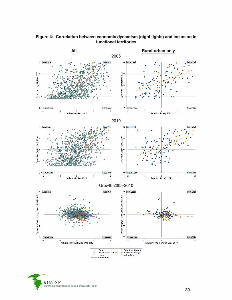
Figure 4: Correlation between economic dynamism (night lights) and inclusion infunctional territories

All Rural-urban only2005

2010

Growth 2005-2010

30

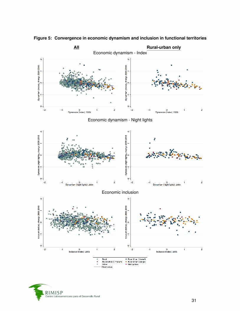
Figure 5: Convergence in economic dynamism and inclusion in functional territories

All Rural-urban onlyEconomic dynamism - Index

Economic dynamism - Night lights

Economic inclusion

31

Table 1: Functional territories in ColombiaDistribution, population, and municipalities by type

(1) (2) (3) (4) (5) (6) (7)Type of territory: Rural Rural-Urban Urban Metropolitan Total

Type 1 Type 2 Type 3Population (thousands): 0 −15 15−60 60−120 120−400 400−600 >600

Municipalities (number) 746 157 61 67 19 71 1121Share 0.66 0.14 0.05 0.05 0.01 0.06 1

Territories (number) 717 98 19 18 3 5 860Share 0.83 0.11 0.02 0.02 0.003 0.01 1

Population 2005 (thousands) 8,929 5,124 2,579 6,347 2,401 17,507 42,888Share 0.2 0.11 0.06 0.14 0.05 0.4 1

32

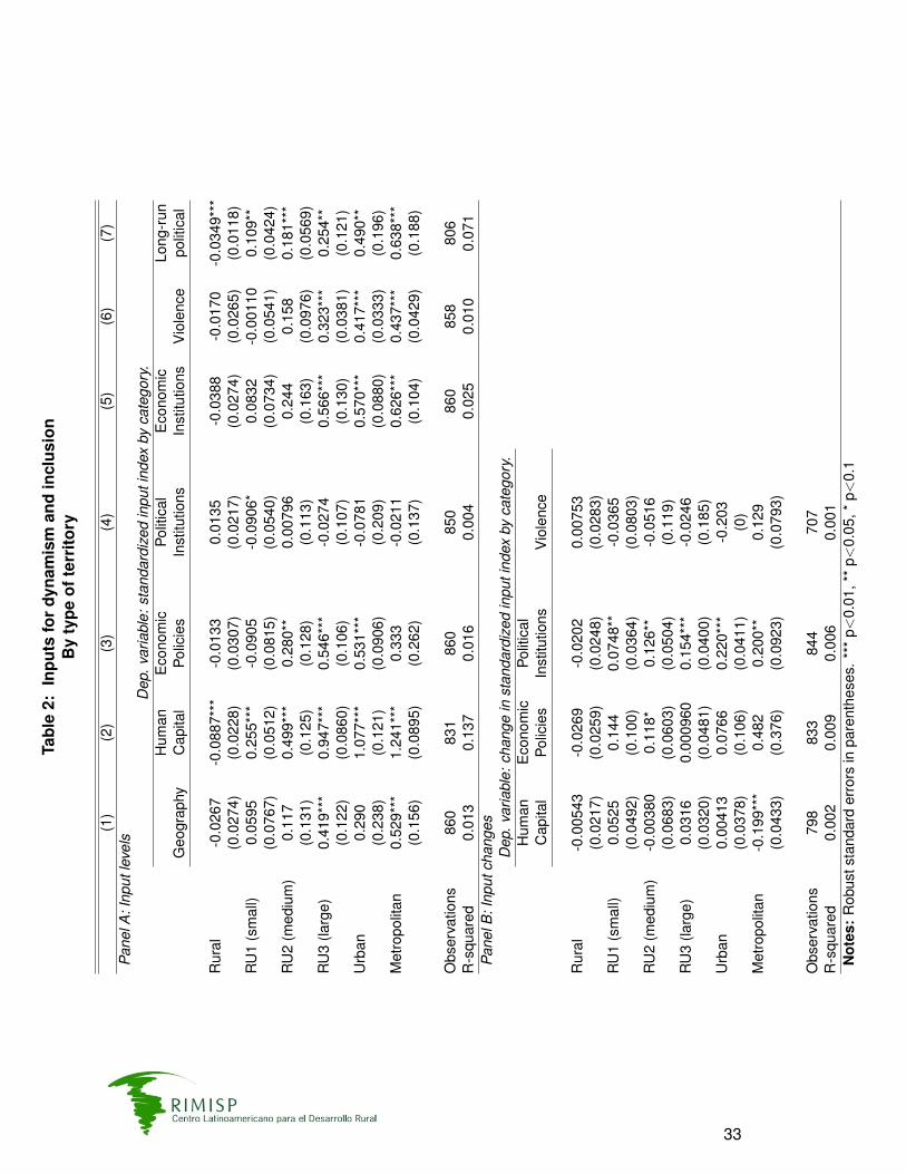
Tabl

e2:

Inpu

tsfo

rdy

nam

ism

and

incl

usio

nB

yty

peof

terr

itory

(1)

(2)

(3)

(4)

(5)

(6)

(7)

Pan

elA

:Inp

utle

vels

Dep

.va

riabl

e:st

anda

rdiz

edin

puti

ndex

byca

tego

ry.

Hum

anE

cono

mic

Polit

ical

Eco

nom

icLo

ng-r

unG

eogr

aphy

Cap

ital

Polic

ies

Inst

itutio

nsIn

stitu

tions

Vio

lenc

epo

litic

al

Rur

al-0

.026

7-0

.088

7***

-0.0

133

0.01

35-0

.038

8-0

.017

0-0

.034

9***

(0.0

274)

(0.0

228)

(0.0

307)

(0.0

217)

(0.0

274)

(0.0

265)

(0.0

118)

RU

1(s

mal

l)0.

0595

0.25

5***

-0.0

905

-0.0

906*

0.08

32-0

.001

100.

109*

*(0

.076

7)(0

.051

2)(0

.081

5)(0

.054

0)(0

.073

4)(0

.054

1)(0

.042

4)R

U2

(med

ium

)0.

117

0.49

9***

0.28

0**

0.00

796

0.24

40.

158

0.18

1***

(0.1

31)

(0.1

25)

(0.1

28)

(0.1

13)

(0.1

63)

(0.0

976)

(0.0

569)

RU

3(la

rge)

0.41

9***

0.94

7***

0.54

6***

-0.0

274

0.56

6***

0.32

3***

0.25

4**

(0.1

22)

(0.0

860)

(0.1

06)

(0.1

07)

(0.1

30)

(0.0

381)

(0.1

21)

Urb

an0.

290

1.07

7***

0.53

1***

-0.0

781

0.57

0***

0.41

7***

0.49

0**

(0.2

38)

(0.1

21)

(0.0

906)

(0.2

09)

(0.0

880)

(0.0

333)

(0.1

96)

Met

ropo

litan

0.52

9***

1.24

1***

0.33

3-0

.021

10.

626*

**0.

437*

**0.

638*

**(0

.156

)(0

.089

5)(0

.262

)(0

.137

)(0

.104

)(0

.042

9)(0

.188

)

Obs

erva

tions

860

831

860

850

860

858

806

R-s

quar

ed0.

013

0.13

70.

016

0.00

40.

025

0.01

00.

071

Pan

elB

:Inp

utch

ange

sD

ep.

varia

ble:

chan

gein

stan

dard

ized

inpu

tind

exby

cate

gory

.H

uman

Eco

nom

icPo

litic

alC

apita

lPo

licie

sIn

stitu

tions

Vio

lenc

e

Rur

al-0

.005

43-0

.026

9-0

.020

20.

0075

3(0

.021

7)(0

.025

9)(0

.024

8)(0

.028

3)R

U1

(sm

all)

0.05

250.

144

0.07

48**

-0.0

365

(0.0

492)

(0.1

00)

(0.0

364)

(0.0

803)

RU

2(m

ediu

m)

-0.0

0380

0.11

8*0.

126*

*-0

.051

6(0

.068

3)(0

.060

3)(0

.050

4)(0

.119

)R

U3

(larg

e)0.

0316

0.00

0960

0.15

4***

-0.0

246

(0.0

320)

(0.0

481)

(0.0

400)

(0.1

85)

Urb

an0.

0041

30.

0766

0.22

0***

-0.2

03(0

.037

8)(0

.106

)(0

.041

1)(0

)M

etro

polit

an-0

.199

***

0.48

20.

200*

*0.

129

(0.0

433)

(0.3

76)

(0.0

923)

(0.0

793)

Obs

erva

tions

798

833

844

707

R-s

quar

ed0.

002

0.00

90.

006

0.00

1N

otes

:R

obus

tsta

ndar

der

rors

inpa

rent

hese

s.**

*p<

0.01

,**

p<0.

05,*

p<0.

1

33

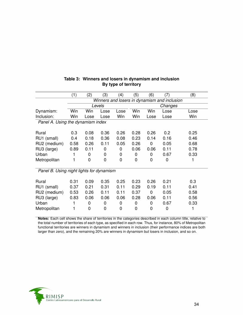
Table 3: Winners and losers in dynamism and inclusionBy type of territory

(1) (2) (3) (4) (5) (6) (7) (8)Winners and losers in dynamism and inclusion

Levels ChangesDynamism: Win Win Lose Lose Win Win Lose LoseInclusion: Win Lose Lose Win Win Lose Lose WinPanel A. Using the dynamism index

Rural 0.3 0.08 0.36 0.26 0.28 0.26 0.2 0.25RU1 (small) 0.4 0.18 0.36 0.08 0.23 0.14 0.16 0.46RU2 (medium) 0.58 0.26 0.11 0.05 0.26 0 0.05 0.68RU3 (large) 0.89 0.11 0 0 0.06 0.06 0.11 0.78Urban 1 0 0 0 0 0 0.67 0.33Metropolitan 1 0 0 0 0 0 0 1

Panel B. Using night lights for dynamism

Rural 0.31 0.09 0.35 0.25 0.23 0.26 0.21 0.3RU1 (small) 0.37 0.21 0.31 0.11 0.29 0.19 0.11 0.41RU2 (medium) 0.53 0.26 0.11 0.11 0.37 0 0.05 0.58RU3 (large) 0.83 0.06 0.06 0.06 0.28 0.06 0.11 0.56Urban 1 0 0 0 0 0 0.67 0.33Metropolitan 1 0 0 0 0 0 0 1

Notes: Each cell shows the share of territories in the categories described in each column title, relative tothe total number of territories of each type, as specified in each row. Thus, for instance, 80% of Metropolitanfunctional territories are winners in dynamism and winners in inclusion (their performance indices are bothlarger than zero), and the remaining 20% are winners in dynamism but losers in inclusion, and so on.

34

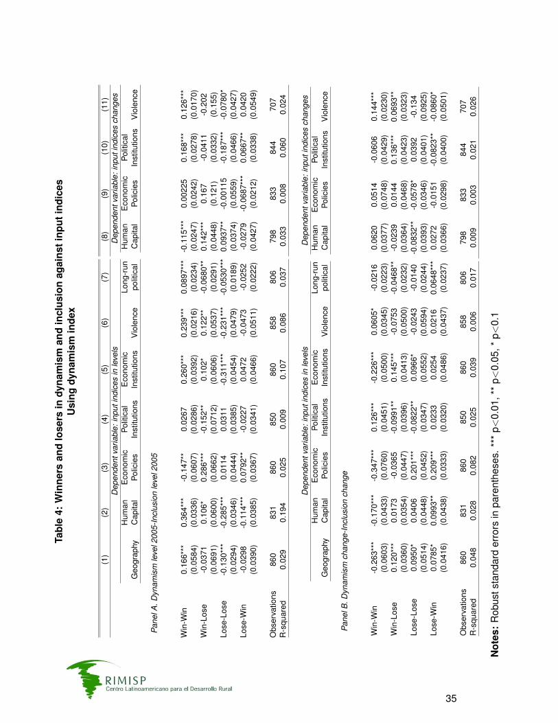
Tabl

e4:

Win

ners

and

lose

rsin

dyna

mis

man

din

clus

ion

agai

nsti

nput

indi

ces

Usi

ngdy

nam

ism

inde

x

(1)

(2)

(3)

(4)

(5)

(6)

(7)

Dep

ende

ntva

riabl

e:in

puti

ndic

esin

leve

lsH

uman

Eco

nom

icPo

litic

alE

cono

mic

Long

-run

Geo

grap

hyC

apita

lPo

licie

sIn

stitu

tions

Inst

itutio

nsV

iole

nce

polit

ical

Pan

elA

.Dyn

amis

mle

vel2

005-

Incl

usio

nle

vel2

005

Win

-Win

0.16

6***

0.36

4***

-0.1

47**

0.02

670.

260*

**0.

239*

**0.

0897

***

(0.0

584)

(0.0

336)

(0.0

607)

(0.0

286)

(0.0

392)

(0.0

216)

(0.0

234)

Win

-Los

e-0

.037

10.

106*

0.28

6***

-0.1

52**

0.10

2*0.

122*

*-0

.068

0**

(0.0

691)

(0.0

600)

(0.0

662)

(0.0

712)

(0.0

606)

(0.0

537)

(0.0

291)

Lose

-Los

e-0

.130

***

-0.2

85**

*0.

0114

0.03

11-0

.311

***

-0.2

31**

*-0

.053

0***

(0.0

294)

(0.0

346)

(0.0

444)

(0.0

385)

(0.0

454)

(0.0

479)

(0.0

189)

Lose

-Win

-0.0

298

-0.1

14**

*0.

0792

**-0

.022

70.

0472

-0.0

473

-0.0

252

(0.0

390)

(0.0

385)

(0.0

367)

(0.0

341)

(0.0

466)

(0.0

511)

(0.0

222)

Obs

erva

tions

860

831

860

850

860

858

806

R-s

quar

ed0.

029

0.19

40.

025

0.00

90.

107

0.08

60.

037

(8)

(9)

(10)

(11)

Dep

ende

ntva

riabl

e:in

puti

ndic

esch

ange

sH

uman

Eco

nom

icPo

litic

alC

apita

lPo

licie

sIn

stitu

tions

Vio

lenc

e

-0.1

15**

*0.

0022

50.

168*

**0.

126*

**(0

.024

7)(0

.024

2)(0

.027

8)(0

.017

0)0.

142*

**0.

167

-0.0

411

-0.2

02(0

.044

8)(0

.121

)(0

.033

2)(0

.155

)0.

0937

**-0

.001

15-0

.187

***

-0.0

780*

(0.0

374)

(0.0

559)

(0.0

466)

(0.0

427)

-0.0

279

-0.0

687*

**0.

0667

**0.

0420

(0.0

427)

(0.0

212)

(0.0

338)

(0.0

549)

798

833

844

707

0.03

30.

008

0.06

00.

024

Dep

ende

ntva

riabl

e:in

puti

ndic

esin

leve

lsH

uman

Eco

nom

icPo

litic

alE

cono

mic

Long

-run

Geo

grap

hyC

apita

lPo

licie

sIn

stitu

tions

Inst

itutio

nsV

iole

nce

polit

ical

Pan

elB

.Dyn

amis

mch

ange

-Incl

usio

nch

ange

Win

-Win

-0.2

63**

*-0

.170

***

-0.3

47**

*0.

126*

**-0

.226

***

0.06

05*

-0.0

216

(0.0

603)

(0.0

433)

(0.0

760)

(0.0

451)

(0.0

500)

(0.0

345)

(0.0

223)

Win

-Los

e0.

120*

**0.

0173

-0.0

365

-0.0

991*

*0.

145*

**-0

.075

3-0

.046

8**

(0.0

360)

(0.0

354)

(0.0

447)

(0.0

396)

(0.0

413)

(0.0

500)

(0.0

232)

Lose

-Los

e0.

0950

*0.

0406

0.20

1***

-0.0

822*

*0.

0966

*-0

.024

3-0

.014

0(0

.051

4)(0

.044

8)(0

.045

2)(0

.034

7)(0

.055

2)(0

.059

4)(0

.024

4)Lo

se-W

in0.

0785

*0.

0993

**0.

209*

**0.

0233

0.02

540.

0216

0.06

48**

*(0

.041

6)(0

.043

8)(0

.033

3)(0

.032

0)(0

.048

6)(0

.043

7)(0

.023

7)

Obs

erva

tions

860

831

860

850

860

858

806

R-s

quar

ed0.

048

0.02

80.

082

0.02

50.

039

0.00

60.

017

Dep

ende

ntva

riabl

e:in

puti

ndic

esch

ange

sH

uman

Eco

nom

icPo

litic

alC

apita

lPo

licie

sIn

stitu

tions

Vio

lenc

e

0.06

200.

0514

-0.0

606

0.14

4***

(0.0

377)

(0.0

748)

(0.0

429)

(0.0

230)

-0.0

239

0.01

440.

136*

**0.

0693

**(0

.036

4)(0

.046

8)(0

.042

3)(0

.032

3)-0

.083

2**

-0.0

578*

0.03

92-0

.134

(0.0

393)

(0.0

346)

(0.0

401)

(0.0

925)

0.02

72-0

.015

1-0

.082

3**

-0.0

860*

(0.0

366)

(0.0

298)

(0.0

400)

(0.0

501)

798

833

844

707

0.00

90.

003

0.02

10.

026

Not

es:

Rob

usts

tand

ard

erro

rsin

pare

nthe

ses.

***

p<0.

01,*

*p<

0.05

,*p<

0.1

35

Tabl

e5:

Win

ners

and

lose

rsin

dyna

mis

man

din

clus

ion

agai

nsti

nput

indi

ces

Usi

ngni

ghtl

ight

sfo

rdy

nam

ism

(1)

(2)

(3)

(4)

(5)

(6)

(7)

Dep

ende

ntva

riabl

e:in

puti

ndic

esin

leve

lsH

uman

Eco

nom

icPo

litic

alE

cono

mic

Long

-run

Geo

grap

hyC

apita

lPo

licie

sIn

stitu

tions

Inst

itutio

nsV

iole

nce

polit

ical

Pan

elA

.Dyn

amis

mle

vel2

005-

Incl

usio

nle

vel2

005

Win

-Win

0.14

6**

0.29

9***

-0.1

56**

*-0

.000

265

0.23

1***

0.24

9***

0.07

09**

*(0

.057

3)(0

.035

4)(0

.060

3)(0

.026

9)(0

.040

3)(0

.024

8)(0

.021

7)W

in-L

ose

-0.0

377

0.09

41*

-0.0

458

-0.3

94**

*-0

.010

70.

105

-0.0

976*

**(0

.041

8)(0

.048

8)(0

.087

7)(0

.046

5)(0

.048

3)(0

.087

5)(0

.030

9)Lo

se-L

ose

-0.1

34**

*-0

.298

***

0.10

7***

0.11

7***

-0.2

92**

*-0

.240

***

-0.0

426*

*(0

.033

7)(0

.036

4)(0

.041

4)(0

.039

9)(0

.048

5)(0

.043

8)(0

.018

6)Lo

se-W

in-0

.003

94-0

.032

20.

0963

***

0.01

540.

0875

*-0

.065

20.

0011

0(0

.041

7)(0

.040

0)(0

.035

9)(0

.037

0)(0

.045

3)(0

.048

1)(0

.026

1)

Obs

erva

tions

860

831

860

850

860

858

806

R-s

quar

ed0.

025

0.15

50.

022

0.06

70.

089

0.09

20.

029

(8)

(9)

(10)

(11)

Dep

ende

ntva

riabl

e:in

puti

ndic

esch

ange

sH

uman

Eco

nom

icPo

litic

alC

apita

lPo

licie

sIn

stitu

tions

Vio

lenc

e

-0.1

24**

*-0

.004

690.

151*

**0.

122*

**(0

.024

5)(0

.023

1)(0

.028

2)(0

.018

3)0.

0631

0.11

6-0

.096

4**

0.01

51(0

.042

2)(0

.120

)(0

.038

3)(0

.049

9)0.

119*

**0.

0094

8-0

.175

***

-0.1

38**

(0.0

387)

(0.0

555)

(0.0

480)

(0.0

581)

-0.0

155

-0.0

604*

**0.

0889

***

0.04

76(0

.042

8)(0

.023

2)(0

.033

4)(0

.054

0)

798

833

844

707

0.03

60.

005

0.05

50.

025

Dep

ende

ntva

riabl

e:in

puti

ndic

esin

leve

lsH

uman

Eco

nom

icPo

litic

alE

cono

mic

Long

-run

Geo

grap

hyC

apita

lPo

licie

sIn

stitu

tions

Inst

itutio

nsV

iole

nce

polit

ical

Pan

elB

.Dyn

amis

mch

ange

-Incl

usio

nch

ange

Win

-Win

-0.1

42**

-0.0

697

-0.2

92**

*0.

0452

-0.1

48**

*0.

124*

**0.

0215

(0.0

665)

(0.0

429)

(0.0

762)

(0.0

408)

(0.0

526)

(0.0

308)

(0.0

278)

Win

-Los

e0.

176*

**0.

0401

0.03

02-0

.140

***

0.21

7***

-0.0

698

-0.0

403*

(0.0

343)

(0.0

342)

(0.0

407)

(0.0

296)

(0.0

382)

(0.0

488)

(0.0

243)

Lose

-Los

e0.

0269

0.01

260.

119*

*-0

.031

80.

0089

4-0

.031

0-0

.021

9(0

.052

3)(0

.046

2)(0

.052

0)(0

.046

8)(0

.057

2)(0

.060

8)(0

.022

6)Lo

se-W

in-0

.038

40.

0110

0.12

3***

0.08

90**

-0.0

531

-0.0

219

0.02

78(0

.040

7)(0

.044

2)(0

.043

3)(0

.036

2)(0

.047

4)(0

.043

1)(0

.020

2)

Obs

erva

tions

860

831

860

850

860

858

806

R-s

quar

ed0.

024

0.00

40.

044

0.02

50.

032

0.01

10.

007

Dep

ende

ntva

riabl

e:in

puti

ndic

esch

ange

sH

uman

Eco

nom

icPo

litic

alC

apita

lPo

licie

sIn

stitu

tions

Vio

lenc

e

0.04

04-0

.034

40.

0147

0.13

6***

(0.0

367)

(0.0

269)

(0.0

373)

(0.0

269)

-0.0

468

0.03

800.

203*

**0.

0731

**(0

.035

2)(0

.046

9)(0

.024

3)(0

.030

2)-0

.054

2-0

.087

6***

-0.0

424

-0.1

38(0

.041

1)(0

.033

5)(0

.056

8)(0

.093

2)0.

0441

0.04

71-0

.132

***

-0.0

605

(0.0

367)

(0.0

593)

(0.0

418)

(0.0

459)

798

833

844

707

0.00

70.

006

0.04

30.

021

Not

es:

Rob

usts

tand

ard

erro

rsin

pare

nthe

ses.

***

p<0.

01,*

*p<

0.05

,*p<

0.1

36

Tabl

e6:

Eco

nom

icdy

nam

ism

and

incl

usio

nin

Col

ombi

a,20

05-2

010

Hum

anca

pita

l

(1)

(2)

(3)

(4)

(5)

(6)

(7)

(8)

(9)

Dep

ende

ntva

riabl

e:G

row

thin

econ

omic

...A

vera

gele

velo

feco

nom

ic...

Dyn

amis

mIn

clus

ion

Dyn

amis

mIn

clus

ion

Inde

xN

ight

light

sIn

dex

Inde

xN

ight

light

sIn

dex

Pan

elA

.“Le

vels

mod

el”(

Initi

alH

uman

Cap

italS

tock

)

Dyn

amis

min

dex

2005

-0.1

78**

*(0

.029

5)N

ight

light

s20

05-0

.081

7***

(0.0

181)

Incl

usio

n20

05-0

.249

***

(0.0

188)

Year

sof

scho

olin

g20

05-0

.093

0***

-0.0

0709

-0.0

584*

**-0

.034

7**

0.05

14**

0.13

0***

0.43

7***

0.39

8***

0.34

3***

(0.0

169)

(0.0

189)

(0.0

138)

(0.0

138)

(0.0

232)

(0.0

233)

(0.0

399)

(0.0

460)

(0.0

366)

Sab

erte

stsc

ores

2005

0.00

544

0.00

625

-0.0

0668

*-0

.006

91**

-0.0

229*

**-0

.006

760.

0072

6-0

.007

480.

0534

***

(0.0

0485

)(0

.004

60)

(0.0

0344

)(0

.003

39)

(0.0

0569

)(0

.005

30)

(0.0

0640

)(0

.009

45)

(0.0

0961

)P

rimar

yen

rollm

entr

ate

2005

0.01

620.

0169

0.00

125

-0.0

310

-0.2

00**

-0.4

26**

*0.

0119

-0.5

83**

*-1

.009

***

(0.0

753)

(0.0

734)

(0.0

597)

(0.0

600)

(0.0

904)

(0.0

823)

(0.1

27)

(0.1

57)

(0.1

55)

Sec

onda

ryen

rollm

entr

ate

2005

0.25

6**

0.32

5***

0.27

3***

0.33

6***

-0.0

958

-0.0

423

0.51

3***

1.26

8***

0.16

7(0

.106

)(0

.109

)(0

.066

2)(0

.071

8)(0

.097

6)(0

.093

7)(0

.143

)(0

.193

)(0

.165

)C

onst

ant

0.22

0-0

.453

*0.

557*

**0.

466*

**0.

986*

**-0

.123

-3.6

73**

*-2

.561

***

-3.9

65**

*(0

.260

)(0

.269

)(0

.170

)(0

.167

)(0

.281

)(0

.273

)(0

.384

)(0

.492

)(0

.504

)

Obs

erva

tions

827

827

827

827

734

734

827

827

734

R-s

quar

ed0.

031

0.10

30.

035

0.05

70.

040

0.22

60.

440

0.36

00.

371

Pan

elB

.“A

ccel

erat

ion

mod

el”(

Gro

wth

inH

uman

Cap

italS

tock

)

Dyn

amis

min

dex

2005

-0.1

27**

*(0

.015

3)N

ight

light

s20

05-0

.078

0***

(0.0

140)

Incl

usio

n20

05-0

.164

***

(0.0

173)

Sab

erte

stsc

ores

2000

-200

50.

134

0.06

52-0

.217

-0.2

880.

0296

-0.1

75-0

.475

-1.4

47**

-1.2

36**

(0.3

27)

(0.3

21)

(0.1

92)

(0.1

97)

(0.3

08)

(0.2

88)

(0.4

03)

(0.5

62)

(0.4

98)

Prim

ary

enro

llmen

trat

e20

00-2

005

-0.0

328

0.00

639

0.08

980.

100

0.22

9**

0.20

9**

0.29

2*0.

245

-0.0

0687

(0.0

865)

(0.0

877)

(0.0

609)

(0.0

612)

(0.0

973)

(0.0

918)

(0.1

74)

(0.2

11)

(0.2

04)

Sec

onda

ryen

rollm

entr

ate

2000

-200

50.

0971

**0.

0514

-0.0

136

-0.0

376

0.06

73*

-0.0

0330

-0.3

10**

*-0

.461

***

-0.3

98**

*(0

.040

8)(0

.041

9)(0

.030

4)(0

.030

2)(0

.038

4)(0

.039

4)(0

.062

4)(0

.078

8)(0

.089

0)C

onst

ant

-0.0

138

0.00

184

0.02

35*

0.09

49**

*0.

0059

00.

0247

0.11

6***

0.16

2***

0.11

8***

(0.0

175)

(0.0

165)

(0.0

134)

(0.0

198)

(0.0

207)

(0.0

199)

(0.0

405)

(0.0

496)

(0.0

431)

Obs

erva

tions

796

796

796

796

707

707

796

796

707

R-s

quar

ed0.

010

0.07

60.

004

0.03

50.

017

0.12

70.

026

0.04

00.

046

Not

es:

Rob

usts

tand

ard

erro

rsin

pare

nthe

ses.

***

p<0.

01,*

*p<

0.05

,*p<

0.1

37

Tabl

e7:

Eco

nom

icdy

nam

ism

and

incl

usio

nin

Col

ombi

a,20

05-2

010

Geo

grap

hy

(1)

(2)

(3)

(4)

(5)

(6)

(7)

(8)

(9)

Dep

ende

ntva

riabl

e:G

row

thin

econ

omic

...A

vera

gele

velo

feco

nom

ic...

Dyn

amis

mIn

clus

ion

Dyn

amis

mIn

clus

ion

Inde

xN

ight

light

sIn

dex

Inde

xN

ight

light

sIn

dex

Dyn

amis

min

dex

2005

-0.2

02**

*(0

.036

6)N

ight

light

s20

05-0

.114

***

(0.0

165)

Incl

usio

n20

05-0

.130

***

(0.0

205)

Land

aptit

ude

inde

x-0

.007

520.

0133

-0.0

0905

0.00

0822

-0.0

0913

-0.0

0403

0.09

94**

*0.

123*

**0.

0347

(0.0

0868

)(0

.009

56)

(0.0

0804

)(0

.008

14)

(0.0

127)

(0.0

122)

(0.0

220)

(0.0

285)

(0.0

226)

Alti

tude

-2.5

1e-0

5*-2

.45e

-05*

*-1

.17e

-05*

-4.3

8e-0

6-1

.73e

-05

1.70

e-06

-9.5

6e-0

68.

86e-

050.

0001

38**

(1.3

2e-0

5)(1

.20e

-05)

(6.3

1e-0

6)(6

.03e

-06)

(1.9

6e-0

5)(1

.22e

-05)

(1.5

4e-0

5)(6

.22e

-05)

(6.1

4e-0

5)D

ista

nce

tone

ares

tcity

0.04

52*

0.04

25*

-0.0

169

-0.0

0892

0.14

1***

0.12

7***

0.00

902

0.09

43-0

.039

7(0

.025

1)(0

.021

8)(0

.017

1)(0

.017

0)(0

.023

8)(0

.022

6)(0

.049

4)(0

.059

8)(0

.050

7)D

ista

nce

tone

ares

tmar

ket

-0.0

0081

3***

-0.0

0092

5***

-0.0

0053

2***

-0.0

0064

4***

0.00

152*

**0.

0011

0***

-0.0

0096

0*-0

.001

71**

*-0

.002

52**

*(0

.000

306)

(0.0

0024

6)(0

.000

154)

(0.0

0016

1)(0

.000

264)

(0.0

0025

8)(0

.000

526)

(0.0

0060

4)(0

.000

595)

Dis

t.B

ogot

a-0

.000

162

-0.0

0034

5**

8.64

e-07

-9.3

1e-0

5-0

.001

18**

*-0

.001

15**

*-0

.000

986*

*-0

.001

21**

-0.0

0038

3(0

.000

185)

(0.0

0015

2)(0

.000

138)

(0.0

0013

8)(0

.000

173)

(0.0

0017

1)(0

.000

399)

(0.0

0048

0)(0

.000

360)

Dis

tanc

eto

near

estfl

uvia

lpor

t0.

0320

**0.

0255

*-0

.012

4-0

.028

2***

-0.0

908*

**-0

.078

6***

-0.0

162

-0.2

10**

*0.

0486

(0.0

163)

(0.0

155)

(0.0

103)

(0.0

107)

(0.0

147)

(0.0

139)

(0.0

272)

(0.0

357)

(0.0

318)

Acc

ess

topr

imar

yro

ads

0.03

440.

100*

**0.

0038

00.

0313

0.01

570.

0361

0.34

2***

0.35

6***

0.16

5***

(0.0

291)

(0.0

315)

(0.0

208)

(0.0

214)

(0.0

287)

(0.0

280)

(0.0

468)

(0.0

616)

(0.0

515)

Par

kar

ea0.

198

-0.0

289

0.22

00.

0335

1.12

2**

1.07

6**

-1.0

24-2

.293

***

0.20

9(0

.479

)(0

.516

)(0

.149

)(0

.153

)(0

.524

)(0

.531

)(0

.745

)(0

.734

)(0

.557

)C

onst

ant

0.00

987

0.01

850.

168*

**0.

288*

**0.

206*

**0.

199*

**0.

0477

0.43

2**

0.04

82(0

.067

8)(0

.057

0)(0

.048

1)(0

.052

9)(0

.072

5)(0

.065

3)(0

.133

)(0

.183

)(0

.165

)

Obs

erva

tions

837

837

837

837

741

741

837

837

741

R-s

quar

ed0.

035

0.17

00.

049

0.10

20.

132

0.18

70.

163

0.22

20.

243

Not

es:

Rob

usts

tand

ard

erro

rsin

pare

nthe

ses.

***

p<0.

01,*

*p<

0.05

,*p<

0.1

38

Tabl

e8:

Eco

nom

icdy

nam

ism

and

incl

usio

nin

Col

ombi

a,20

05-2

010

Eco

nom

icpo

licie

s

(1)

(2)

(3)

(4)

(5)

(6)

(7)

(8)

(9)

Dep

ende

ntva

riabl

e:G

row

thin

econ

omic

...A

vera

gele

velo

feco

nom

ic...

Dyn

amis

mIn

clus

ion

Dyn

amis

mIn

clus

ion

Inde

xN

ight

light

sIn

dex

Inde

xN

ight

light

sIn

dex

Pan

elA

.“Le

vels

mod

el”(

Initi

alpo

licie

s)

Dyn

amis

min

dex

2005

-0.2

13**

*(0

.040

4)N

ight

light

s20

05-0

.070

4***

(0.0

141)

Incl

usio

n20

05-0

.174

***

(0.0

168)

Sav

ing

rate

2005

-0.0

0472

***

-0.0

0263

***

-0.0

0213

***

-0.0

0177

***

0.00

0418

0.00

156*

*0.

0074

1***

0.00

640*

**0.

0068

1***

(0.0

0084

0)(0

.000

787)

(0.0

0062

1)(0

.000

613)

(0.0

0076

0)(0

.000

753)

(0.0

0124

)(0

.001

60)

(0.0

0140

)Tr

ansf

ers

inco

me

-0.0

0275

-0.0

0682

***

-0.0

0077

4-0

.001

28*

0.00

0977

-0.0

0079

2-0

.020

5***

-0.0

109*

**-0

.009

70**

*(0

.001

77)

(0.0

0209

)(0

.000

667)

(0.0

0067

4)(0

.000

927)

(0.0

0087

4)(0

.001

72)

(0.0

0211

)(0

.001

88)

Inve

stm

entr

ate

2005

0.00

599*

0.00

310

-7.0

0e-0

5-0

.001

010.

0012

1-0

.000

806

-0.0

105

-0.0

197*

**-0

.011

0*(0

.003

30)

(0.0

0272

)(0

.001

38)

(0.0

0137

)(0

.001

79)

(0.0

0137

)(0

.006

92)

(0.0

0637

)(0

.005

87)

Con

stan

t-0

.157

0.32

4*0.

122

0.28

4***

-0.1

830.

0815

2.17

5***

2.25

3***

1.43

0***

(0.2

25)

(0.1

86)

(0.1

03)

(0.1

09)

(0.1

36)

(0.0

977)

(0.5

85)

(0.5

23)

(0.4

88)

Obs

erva

tions

838

838

838

838

742

742

838

838

742

R-s

quar

ed0.

052

0.17

20.

022

0.04

50.

004

0.12

60.

326

0.10

70.

112

Pan

elB

.“A

ccel

erat

ion

mod

el”(

Impr

ovem

enti

nPo

licie

s)

Dyn

amis

min

dex

2005

-0.1

75**

*(0

.031

3)N

ight

light

s20

05-0

.067

2***

(0.0

133)

Incl

usio

n20

05-0

.161

***

(0.0

163)

Sav

ing

rate

2005

-201

00.

0002

836.

99e-

05-0

.000

170*

**-0

.000

218*

**0.

0003

12**

*0.

0002

80**

*-0

.001

07**

*-0

.001

12**

*-4

.69e

-05

(0.0

0018

3)(0

.000

181)

(5.6

3e-0

5)(6

.23e

-05)

(6.6

9e-0

5)(5

.73e

-05)

(0.0

0012

7)(0

.000

232)

(0.0

0032

0)Tr

ansf

ers

inco

me

2005

-201

00.

0627

0.08

25*

-0.0

0446

-0.0

0884

0.01

58-5

.46e

-05

0.14

4***

-0.0

983*

-0.0

904

(0.0

502)

(0.0

489)

(0.0

120)

(0.0

111)

(0.0

186)

(0.0

134)

(0.0

451)

(0.0

550)

(0.0

585)

Inve

stm

entr

ate

2005

-201

00.

239

0.35

60.

120*

0.14

6**

0.03

190.

0053

80.

788*

**0.

636*

*-0

.149

(0.3

10)

(0.2

83)

(0.0

615)

(0.0

583)

(0.1

00)

(0.1

09)

(0.1

71)

(0.2

79)

(0.2

35)

Con

stan

t-0

.016

8-0

.022

1-0

.004

400.

0497

***

-0.0

0452

-0.0

0160

-0.0

387

-0.0

150

0.01

59(0

.016

1)(0

.015

3)(0

.010

8)(0

.015

8)(0

.015

1)(0

.014

5)(0

.027

2)(0

.036

0)(0

.031

6)

Obs

erva

tions

833

833

833

833

736

736

833

833

736

R-s

quar

ed0.

014

0.13

00.

003

0.02

60.

001

0.11

70.

031

0.01

00.

006

Not

es:

Rob

usts

tand

ard

erro

rsin

pare

nthe

ses.

***

p<0.

01,*

*p<

0.05

,*p<

0.1

39

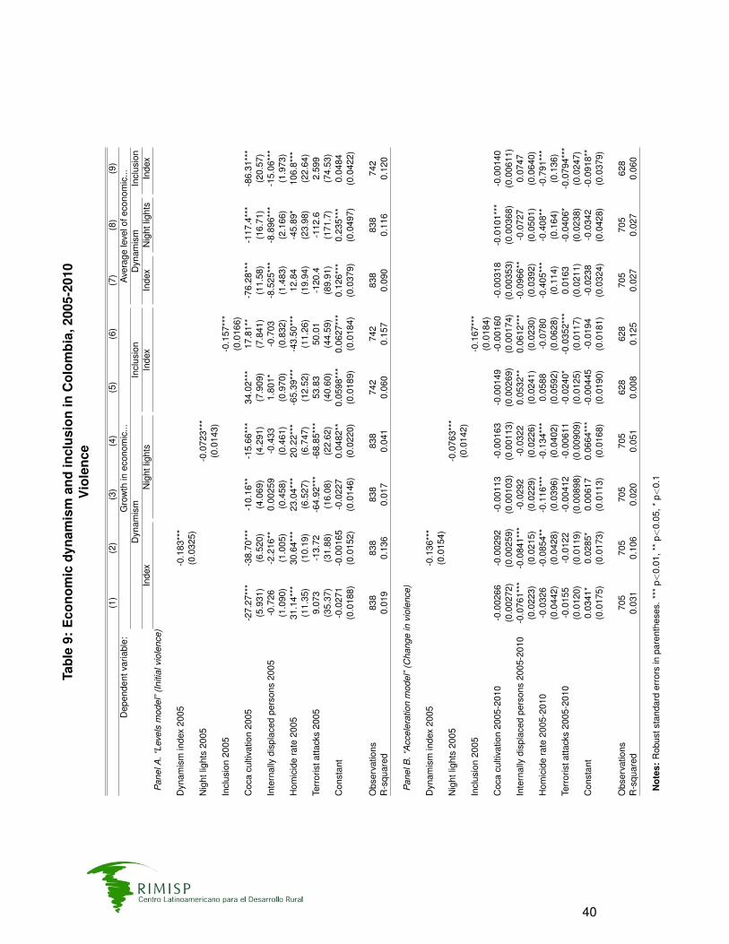
Tabl

e9:

Eco

nom

icdy

nam

ism

and

incl

usio

nin

Col

ombi

a,20

05-2

010

Vio

lenc

e

(1)

(2)

(3)

(4)

(5)

(6)

(7)

(8)

(9)

Dep

ende

ntva

riabl

e:G

row

thin

econ

omic

...A

vera

gele

velo

feco

nom

ic...

Dyn

amis

mIn

clus

ion

Dyn

amis

mIn

clus

ion

Inde

xN

ight

light

sIn

dex

Inde

xN

ight

light

sIn

dex

Pan

elA

.“Le

vels

mod

el”(

Initi

alvi

olen

ce)

Dyn

amis

min

dex

2005

-0.1

83**

*(0

.032

5)N

ight

light

s20

05-0

.072

3***

(0.0

143)

Incl

usio

n20

05-0

.157

***

(0.0

166)

Coc

acu

ltiva

tion

2005

-27.

27**

*-3

8.70

***

-10.

16**

-15.

66**

*34

.02*

**17

.81*

*-7

6.28

***

-117

.4**

*-8

6.31

***

(5.9

31)

(6.5

20)

(4.0

69)

(4.2

91)

(7.9

09)

(7.8

41)

(11.

58)

(16.

71)

(20.

57)

Inte

rnal

lydi

spla

ced

pers

ons

2005

-0.7

26-2

.216

**0.

0025

9-0

.433

1.80

1*-0

.703

-8.5

25**

*-8

.896

***

-15.

06**

*(1

.090

)(1

.005

)(0

.458

)(0

.461

)(0

.970

)(0

.832

)(1

.483

)(2

.166

)(1

.973

)H

omic

ide

rate

2005

31.1

4***

30.6

4***

23.0

4***

20.2

2***

-65.

39**

*-4

3.50

***

12.8

4-4

5.89

*10

6.8*

**(1

1.35

)(1

0.19

)(6

.527

)(6

.747

)(1

2.52

)(1

1.26

)(1

9.94

)(2

3.98

)(2

2.64

)Te

rror

ista

ttack

s20

059.

073

-13.

72-6

4.92

***

-68.

85**

*53

.83

50.0

1-1

20.4

-112

.62.

599

(35.

37)

(31.

88)

(16.

08)

(22.

62)

(40.

60)

(44.

59)

(89.

91)

(171

.7)

(74.

53)

Con

stan

t-0

.027

1-0

.001

65-0

.022

70.

0482

**0.

0598

***

0.06

27**

*0.

126*

**0.

235*

**0.

0484

(0.0

188)

(0.0

152)

(0.0

146)

(0.0

220)

(0.0

189)

(0.0

184)

(0.0

379)

(0.0

497)

(0.0

422)

Obs

erva

tions

838

838

838

838

742

742

838

838

742

R-s

quar

ed0.

019

0.13

60.

017

0.04

10.

060

0.15

70.

090

0.11

60.

120

Pan

elB

.“A

ccel

erat

ion

mod

el”(

Cha

nge

invi

olen

ce)

Dyn

amis

min

dex

2005

-0.1

36**

*(0

.015

4)N

ight

light

s20

05-0

.076

3***

(0.0

142)

Incl

usio

n20

05-0

.167

***

(0.0

184)

Coc

acu

ltiva

tion

2005

-201

0-0

.002

66-0

.002

92-0

.001

13-0

.001

63-0

.001

49-0

.001

60-0

.003

18-0

.010

1***

-0.0

0140

(0.0

0272

)(0

.002

59)

(0.0

0103

)(0

.001

13)

(0.0

0269

)(0

.001

74)

(0.0

0353

)(0

.003

68)

(0.0

0611

)In

tern

ally

disp

lace

dpe

rson

s20

05-2

010

-0.0

761*

**-0

.084

1***

-0.0

292

-0.0

322

0.05

32**

0.06

12**

*-0

.096

6**

-0.0

727

0.07

47(0

.022

3)(0

.021

5)(0

.022

9)(0

.022

6)(0

.024

1)(0

.023

0)(0

.039

2)(0

.050

1)(0

.064

0)H

omic

ide

rate

2005

-201

0-0

.032

6-0

.085

4**

-0.1

16**

*-0

.134

***

0.05

88-0

.078

0-0

.405

***

-0.4

08**

-0.7

91**

*(0

.044

2)(0

.042

8)(0

.039

6)(0

.040

2)(0

.059

2)(0

.062

8)(0

.114

)(0

.164

)(0

.136

)Te

rror

ista

ttack

s20

05-2

010

-0.0

155

-0.0

122

-0.0

0412

-0.0

0611

-0.0

240*

-0.0

352*

**0.

0163

-0.0

406*

-0.0

794*

**(0

.012

0)(0

.011

9)(0

.008

98)

(0.0

0909

)(0

.012

5)(0

.011

7)(0

.021

1)(0

.023

8)(0

.024

7)C

onst

ant

0.03

41*

0.02

85*

0.00

617

0.06

64**

*-0

.004

45-0

.019

4-0

.023

8-0

.034

2-0

.091

8**

(0.0

175)

(0.0

173)

(0.0

113)

(0.0

168)

(0.0

190)

(0.0

181)

(0.0

324)

(0.0

428)

(0.0

379)

Obs

erva

tions

705

705

705

705

628

628

705

705

628

R-s

quar

ed0.

031

0.10

60.

020

0.05

10.

008

0.12

50.

027

0.02

70.

060

Not

es:

Rob

usts

tand

ard

erro

rsin

pare

nthe

ses.

***

p<0.

01,*

*p<

0.05

,*p<

0.1

40

Tabl

e10

:E

cono

mic

dyna

mis

man

din

clus

ion

inC

olom

bia,

2005

-201

0E

cono

mic

Inst

itutio

ns

(1)

(2)

(3)

(4)

(5)

(6)

(7)

(8)

(9)

Dep

ende

ntva

riabl

e:G

row

thin

econ

omic

...A

vera

gele

velo

feco

nom

ic...

Dyn

amis

mIn

clus

ion

Dyn

amis

mIn

clus

ion

Inde

xN

ight

light

sIn

dex

Inde

xN

ight

light

sIn

dex

Dyn

amis

min

dex

2005

-0.2

05**

*(0

.034

7)N

ight

light

s20

05-0

.099

0***

(0.0

152)

Incl

usio

n20

05-0

.152

***

(0.0

183)

Ope

nG

over

nmen

tInd

exIG

A0.

0029

50.

0062

4***

2.14

e-05

0.00

0891

-0.0

0038

00.

0019

40.

0175

***

0.01

30**

*0.

0150

***

(0.0

0182

)(0

.001

94)

(0.0

0092

9)(0

.000

939)

(0.0

0133

)(0

.001

36)

(0.0

0240

)(0

.003

02)

(0.0

0285

)La

nds

info

rmal

ityra

te0.

398

-2.0

72**

-1.7

72**

*-2

.885

***

3.97

8***

1.64

1**

-11.

84**

*-1

7.47

***

-13.

34**

*(0

.820

)(0

.806

)(0

.422

)(0

.484

)(0

.702

)(0

.750

)(1

.031

)(1

.226

)(1

.345

)C

onst

ant

-0.1

56*

-0.2

82**

*0.

0280

0.08

28*

-0.0

472

-0.1

26*

-0.6

93**

*-0

.371

**-0

.539

***

(0.0

941)

(0.0

969)

(0.0

481)

(0.0

479)

(0.0

729)

(0.0

729)

(0.1

21)

(0.1

61)

(0.1

57)

Obs

erva

tions

838

838

838

838

742

742

838

838

742

R-s

quar

ed0.

006

0.14

10.

014

0.05

70.

041

0.12

50.

182

0.16

10.

180

Not

es:

Rob

usts

tand

ard

erro

rsin

pare

nthe

ses.

***

p<0.

01,*

*p<

0.05

,*p<

0.1

41

Tabl

e11

:E

cono

mic

dyna

mis

man

din

clus

ion

inC

olom

bia,

2005

-201

0Po

litic

alin

stitu

tions

(1)

(2)

(3)

(4)

(5)

(6)

(7)

(8)

(9)

Dep

ende

ntva

riabl

e:G

row

thin

econ

omic

...A

vera

gele

velo

feco

nom

ic...

Dyn

amis

mIn

clus

ion

Dyn

amis

mIn

clus

ion

Inde

xN

ight

light

sIn

dex

Inde

xN

ight

light

sIn

dex

Pan

elA

.“Le

vels

mod

el”(

Initi

alpo

litic

aleq

uilib

rium

)

Dyn

amis

min

dex

2005

-0.1

66**

*(0

.032

2)N

ight

light

s20

05-0

.083

7***

(0.0

139)

Incl

usio

n20

05-0

.148

***

(0.0

169)

Judg

espe

rcap

ita20

050.

0033

1**

0.00

331*

**-0

.001

90*

-0.0

0213

**-0

.007

18**

*-0

.004

87**

*0.

0016

6-0

.005

07*

0.01

21**

*(0

.001

33)

(0.0

0127

)(0

.001

08)

(0.0

0108

)(0

.001

61)

(0.0

0157

)(0

.002

11)

(0.0

0276

)(0

.002

81)

Par

apol

itici

anvo

tes

2006

0.04

590.

0397

0.08

39**

0.09

72**

-0.1

86**

*-0

.198

***

-0.0

148

0.27

6**

-0.1

74(0

.054

3)(0

.053

2)(0

.042

6)(0

.042

0)(0

.054

9)(0

.051

7)(0

.095

8)(0

.120

)(0

.109

)Pe

rson

alvo

tein

Hou

se20

06-0

.104

-0.0

0120

0.08

07**

0.15

9***

-0.2

59**

*-0

.046

80.

568*

**1.

414*

**1.

307*

**(0

.114

)(0

.125

)(0

.039

3)(0

.043

4)(0

.070

8)(0

.069

7)(0

.149

)(0

.119

)(0

.124

)Pe

rson

alvo

tein

Sen

ate

2006

0.45

4*0.

303

-0.0

547

-0.0

640

-0.2

10-0

.334

*-0

.686

-0.1

92-0

.944

*(0

.236

)(0

.211

)(0

.121

)(0

.127

)(0

.214

)(0

.191

)(0

.435

)(0

.486

)(0

.490

)C

onst

ant

-0.3

69*

-0.3

19**

-0.0

353

-0.0

257

0.56

4***

0.47

8***

0.11

8-1

.050

***

-0.3

04(0

.201

)(0

.161

)(0

.090

2)(0

.093

1)(0

.154

)(0

.142

)(0

.341

)(0

.356

)(0

.371

)

Obs

erva

tions

837

837

837

837

741

741

837

837

741

R-s

quar

ed0.

014

0.11

70.

013

0.04

60.

072

0.15

50.

021

0.10

10.

140

Pan

elA

.“A

ccel

erat

ion

mod

el”(

Cha

nges

inpo

litic

aleq

uilib

rium

)

Dyn

amis

min

dex

2005

-0.1

88**

*(0

.032

1)N

ight

light

s20

05-0

.091

0***

(0.0

136)

Incl

usio

n20

05-0

.132

***

(0.0

177)

Par

apol

itici

anvo

tes

2006

-201

4-0

.009

38**

*-0

.013

2***

-0.0

136*

**-0

.015

4***

0.00

252

0.00

109

-0.0

248*

**-0

.035

8***

-0.0

0961

(0.0

0314

)(0

.003

06)

(0.0

0371

)(0

.003

66)

(0.0

0371

)(0

.003

72)

(0.0

0421

)(0

.006

80)

(0.0

0856

)Pe

rson

alvo

tein

Hou

se20

06-2

014

0.00

189

7.90

e-05

-0.0

0242

***

-0.0

0358

***

0.00

232

0.00

0887

-0.0

0871

***

-0.0

201*

**-0

.009

71**

*(0

.002

61)

(0.0

0266

)(0

.000

862)

(0.0

0101

)(0

.001

70)

(0.0

0133

)(0

.002

00)

(0.0

0368

)(0

.003

11)

Pers

onal

vote

inS

enat

e20

06-2

014

-0.2

29**

*-0

.374

***

-0.2

36**

*-0

.274

***

0.57

9***

0.34

7***

-0.8

83**

*-0

.742

***

-1.4

72**

*(0

.081

0)(0

.084

1)(0

.049

6)(0

.050

9)(0

.083

3)(0

.085

1)(0

.136

)(0

.172

)(0

.153

)C

onst

ant

-0.0

248

-0.0

380*

*-0

.019

3*0.

0524

***

0.06

40**

*0.

0388

**-0

.082

5***

-0.0

487

-0.1

59**

*(0

.016

9)(0

.016

0)(0

.010

9)(0

.015

6)(0

.016

6)(0

.016

8)(0

.027

5)(0

.037

5)(0

.031

8)

Obs

erva

tions

837

837

837

837

741

741

837

837

741

R-s

quar

ed0.

018

0.14

60.

053

0.09

30.

076

0.14

10.

072

0.06

60.

132

Not

es:

Rob

usts

tand

ard

erro

rsin

pare

nthe

ses.

***

p<0.

01,*

*p<

0.05

,*p<

0.1

42

Table 12: Economic dynamism and inclusion in Colombia, 2005-2010Longer-run determinants

(1) (2) (3)Dependent variable: Average level of economic...

Dynamism InclusionIndex Night lights Index

Alcabala -0.227* -0.140 0.216(0.118) (0.152) (0.159)

Mail 0.129 0.0520 0.126(0.135) (0.172) (0.139)

Aguardiente 0.536*** 0.551*** 0.229***(0.112) (0.116) (0.0751)

Local level FT employees 1995 6.26e-05 8.04e-06 -0.000121***(5.06e-05) (7.20e-05) (4.29e-05)

Government officials 1794 0.00229*** -0.00108 0.00809***(0.000665) (0.00136) (0.00108)

Public officials 1918 0.000137 0.000255 0.000120(0.000118) (0.000186) (0.000160)

Informality of property rights -14.83*** -21.10*** -15.19***(1.194) (1.359) (1.427)

Slavery 1843 TF 2.555*** 3.402** -1.240(0.936) (1.318) (0.942)

Constant 0.226*** 0.294*** 0.218***(0.0455) (0.0572) (0.0466)

Observations 791 791 699R-squared 0.215 0.208 0.196Notes: Robust standard errors in parentheses. *** p<0.01, ** p<0.05, * p<0.1

43

A Appendix Tables

Table A-1: Variable description and sources

Variable Description Source

Dynamism index,2005 and 2010

Average of territorial standardized night lights and per capita tax revenue

Night lights, 2005 and2010

Total light intensity (sum of all light pixels in each territory) divided bytotal area (sum of the area of all municipalities in the territory) in km2.We take the log of (1 plus) given a very skewed distribution in levels(and to allow for some territories with zero light). Finally we standardizeeach year for regressions and for the dynamism index.

Defense MeteorologicalSatellite Program’s Op-erational Linescan Sys-tem (DMSP-OLS)

Tax Revenue percapita, 2005 and 2010

Total tax revenue by territory (in 2010 pesos) divided by population. Wetake the log of (1 plus) the ratio and standardize for the dynamism index.

National Planning De-partment, DNP

Inclusion index, 2005and 2010

Average of territorial standardized child mortality, proportion of people in Sisben 1category (poor), and share of low-weight births

Child mortality rate,2005 and 2010

Standardized weighted average (by population) of child mortality ratefor municipalities in the territory.

National Statistical In-stitute, DANE

Share in Sisben 1, 2005and 2010

Standardized population share in Sisben category 1 in the territory. TheSystem of Beneficiary Selection (also known as Census of the Poor)assigns a poverty index for each family to identify the poorest. Category1 is the poorest tier.

Census of the poor,SISBEN

Share of low-weightbirths, 2005 and 2010

Standardized share of births that are in low weight (2,499 grams or less,regardless of gestional age) in the territory

Vital Statistics, NationalStatistical Institute,DANE

GeographyLand aptitude index Derived from an index of soil aptitude where 1 is the most suitable and

level 8 the lest suitable (inverted to ease interpretation), and computedas the average aptitude of solid in the territory

National Geographic In-stitute, IGAC

Distance to nearest city Average Euclidean distance of municipalities in each territory to theclosest metropolis (top 3 largest cities, Bogota, Cali and Medellın)

Own estimation

Distance to nearestmarket

Average Euclidean distance of municipalities in each territory to theclosest wholesales market

AGRONET

Distance to nearest flu-vial port

Average Euclidean distance of municipalities in each territory to theclosest city with fluvial port, namely, Barranquilla, Buenaventura, Carta-gena and Santa Marta

Own estimation

Access to primaryroads

Proportion of municipalities in territory with access to main highway net-work (primary roads)

Pachon and Ramırez(2006)

EducationPrimary enrollmentrate, 2005 and 2010

Primary Gross Enrollment Rate. Primary Gross Enrollment Rate is thetotal enrollment in primary like proportion of population in territory be-tween 6 and 11 years

SIMAT of Ministry ofEducation

Continues in the next page

44

Table A-1 – Variable description (continued from last page)

Variable Description SourceSecondary enrollmentrate, 2005 and 2010

Secondary Gross Enrollment Rate. Secondary Gross Enrollment Rateis the total enrollment in secondary like proportion of population in terri-tory between 12 and 17 years

SIMAT of Ministry ofEducation

Years of schooling,2005

Weighted average (by population) of municipal years of schoolingamong people older than 15 year

National Census 2005,National Statistical In-stitute, DANE

Saber test scores, 2005and 2010

Weighted average (by population) of municipal scores in the officialstandardized tests (average from mathematics, language, social sci-ences, philosophy and biology).

Colombian Institute forEducation and Evalua-tion, ICFES

Economic policiesSaving rate, 2005 and2010

Weighted average (by population) of municipal savings relative to cur-rent income.

National Panning De-partment, DNP

Investment reate, 2005and 2010

Weighted average (by population) of municipal savings relative to cur-rent expenditure.

National Panning De-partment, DNP

Economic institutionsInformality of propertyrights

Proportion of land without a title or registration. Average from 2000 to2006

National Geographic In-stitute Agustın Codazzi,IGAC

Open Government In-dex IGA

Weighted average (by population) of municipal index in the territory.IGA Index is a synthetic indicator that measures the performance ofstrategic anti-corruption standards according to the following 24 indica-tors grouped in eight categories: (i) Internal control: Standard Modelof Internal Control (MECI), Internal Accounting Control; (ii) Documentmanagement: Law of Archives; (iii) Recruitment: Annual ProcurementPlan, Contract Publishing; (iv) Territorial core competences: Single In-formation System (SUI), Social Programs (SISBEN), Integrated LicenseSystem, Hospital Information System (SIHO); (v) Administrative and fi-nancial management systems: Unique Territorial Form (FUT), Royal-ties, Budget Execution System (SICEP), Public Employment Informa-tion and Management System (SIGEP), Information and Asset Man-agement System (SIGA); (vi) Transparency and accountability: SICEPAnti-corruption, SICEP Risk Map, SICEP Control and follow up, SICEPAccountability; (vii) SICEP Citizen Support; (viii) Electronic governmentcapacity: GEL Open Government, GEL Services, SICEP Open Data,SICEP Advertising, Unique Procedures Information System (SUIT). Fora more detailed explanation of the indicators, please visit: https://

www.procuraduria.gov.co/portal/indicadores IGA.page

Procuradurıa General(Inspector General)

Political institutions/political equilibriumJudges per capita,2005

Weighted average (by population) of municipal judges per 100.000 in-habitants

Villegas and R. (2013)

Continues in the next page

45

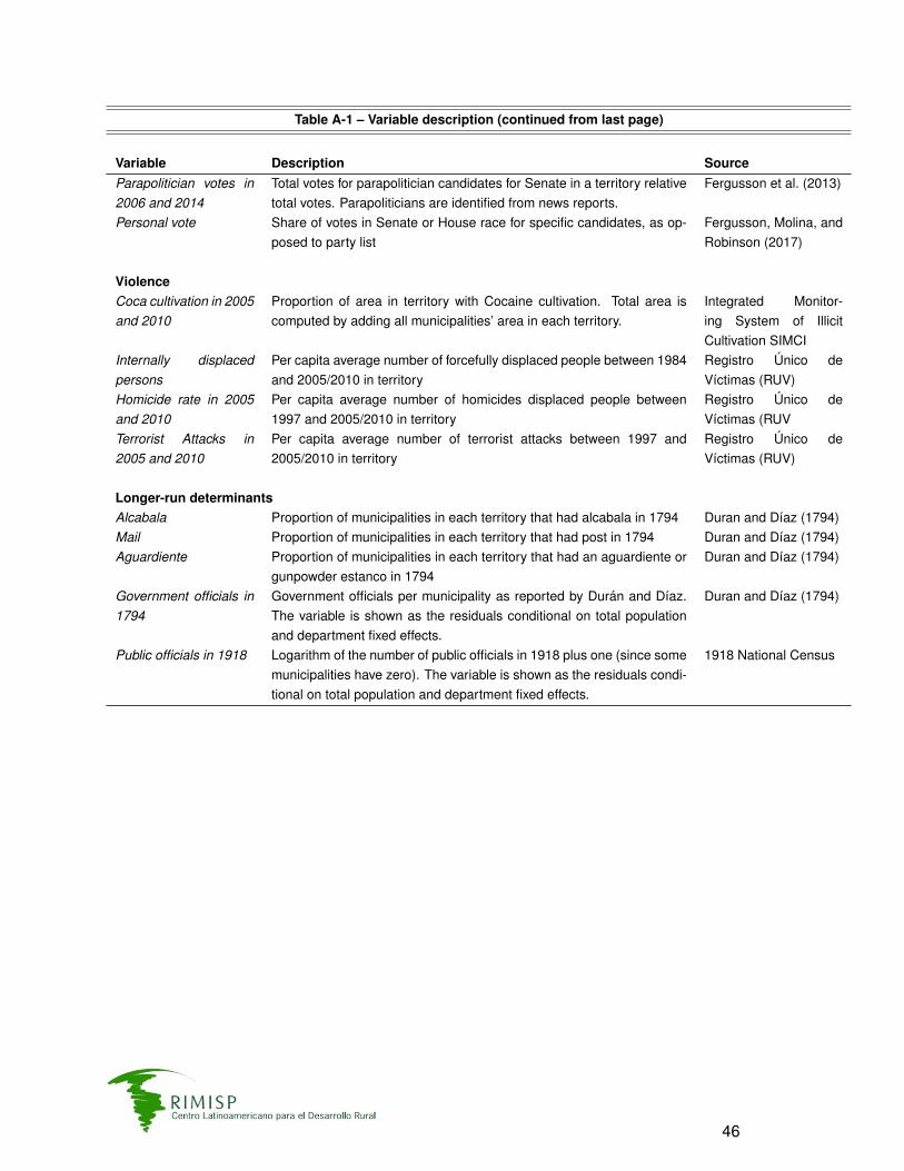
Table A-1 – Variable description (continued from last page)

Variable Description SourceParapolitician votes in2006 and 2014

Total votes for parapolitician candidates for Senate in a territory relativetotal votes. Parapoliticians are identified from news reports.

Fergusson et al. (2013)

Personal vote Share of votes in Senate or House race for specific candidates, as op-posed to party list

Fergusson, Molina, andRobinson (2017)

ViolenceCoca cultivation in 2005and 2010

Proportion of area in territory with Cocaine cultivation. Total area iscomputed by adding all municipalities’ area in each territory.

Integrated Monitor-ing System of IllicitCultivation SIMCI

Internally displacedpersons

Per capita average number of forcefully displaced people between 1984and 2005/2010 in territory

Registro Unico deVıctimas (RUV)

Homicide rate in 2005and 2010

Per capita average number of homicides displaced people between1997 and 2005/2010 in territory

Registro Unico deVıctimas (RUV

Terrorist Attacks in2005 and 2010

Per capita average number of terrorist attacks between 1997 and2005/2010 in territory

Registro Unico deVıctimas (RUV)

Longer-run determinantsAlcabala Proportion of municipalities in each territory that had alcabala in 1794 Duran and Dıaz (1794)Mail Proportion of municipalities in each territory that had post in 1794 Duran and Dıaz (1794)Aguardiente Proportion of municipalities in each territory that had an aguardiente or

gunpowder estanco in 1794Duran and Dıaz (1794)

Government officials in1794

Government officials per municipality as reported by Duran and Dıaz.The variable is shown as the residuals conditional on total populationand department fixed effects.

Duran and Dıaz (1794)

Public officials in 1918 Logarithm of the number of public officials in 1918 plus one (since somemunicipalities have zero). The variable is shown as the residuals condi-tional on total population and department fixed effects.

1918 National Census

46