Growing Artificial Societies - Carleton University
49
1 Growing Artificial Societies Social Science from the Bottom Up presentation by Ian Nunn
Transcript of Growing Artificial Societies - Carleton University

1
Growing Artificial Societies
Social Science from the Bottom Uppresentation by
Ian Nunn

2
Lecture Based On
• Book: Growing Artificial Societies by Joshua Epstein and Robert Axtell
• Software: – Ascape, Sugarscape derivative
www.brookings.edu/dynamics/models/ascape/
– StarLogo Sugarscape demo el.www.media.mit.edu/groups/el/Projects/starlogo/
• All figures reproduced from the book

3
Major Discussion Topics
• Traditional vs. Agent-Based simulations
• Introduction to the Sugarscape (Ascape) computer model
• Presentation of elementary social simulations
• Study of models of economic trade

4
A Fundamental Question for Social Science:
• How does the heterogeneous behavior of individual actors or agents generate the global macroscopic regularities of social phenomena– group formation, migration and other
population dynamics
– group activities: warfare and trade
– transmission of culture and disease

5
Characteristics of Traditional Social Simulation Techniques
• Top down approach
• Based on departmentalization: economics, demographics, political science, epidemiology
• Theoretical basis: game theory, general equilibrium theory
• Mathematical tools: statistical estimating and modeling, differential equations
• Focus: deriving notions of equilibria stability

6
Characteristics of TraditionalSocial Simulation Models
• Rational actor: infinite computing capability, infinite lifetime, maximizes a static exogenous utility function
• Homogeneous populations and sub-populations
• Inability to model coupling between different social science disciplines

7
New Approach: Agent-Based Modeling
• Origin: Thomas Schelling’s work (1969+)
• Based on Multi-agent systems
• Also known as Artificial Societies: Builder and Banks (1991)

8
Thesis of the Approach
Fundamental social structures and group behaviors emerge from the interaction of individual agents operating on artificial environments under rules that place only bounded demands on each agent’s information and computational capacity.
- Growing Artificial Societies, Epstein and Axtell

9
Characteristics of Agent-Based Social Simulation Techniques
• Bottom up approach
• Modeled on particle swarm or agent systems– a set of agents
– an environment or space they operate in
– sets of behavioral rules
– local expression of properties or attributes
• Manifest out-of equilibrium dynamics

10
The Sugarscape Model (Epstein and Axtell)
• A two-dimensional lattice representing an environment in which agents move and act according to rules of behavior
• Environment: the set of all lattice points each having a sugar level and capacity
• Initial Environment: two sugar mountains (NE & SW), two deserts (NW & SE)

11
The Sugarscape Model (cont.)
• Initial state variables and fixed parameters may be randomly selected on fixed domains
• Environment behavior governed by a set of rules E
• Agent behavior governed by a set of rules A
• An artificial society is modeled by the pair (E, A)

12
Some Social Behavior Modeled in Sugarscape
Discussed in this lecture:
• movement and resource gathering
• pollution
• sexual reproduction and inheritance
• cultural transmission
• trade and economic markets
Not discussed in this lecture:
• combat, credit, immune learning, disease propagation

13
The Environment
• Primarily passive in expression
• Basic internal state (parameters)– (renewable) resource (sugar) level r : (variable)
– resource (sugar) capacity c: (fixed)
– growback rate α per unit time: (fixed)
• Basic rule of behavior– sugar growback rule Gá: at each lattice position
for each time interval rt ← rt-1 + α s.t. rt ≤ c

14
The Agent
• Active in expression
• Basic internal state (fixed parameters) – vision: random distance v it can see (NEWS)
– metabolism: random amount of sugar m burnt per round
• Basic internal state (variables) – sugar accumulation: (initial) level a
– location: random grid position (x,y)

15
The Agent (cont.)
• Basic rule of behavior– agent movement (resource gathering) rule M:
• find the first, closest unoccupied site with max(r) within distance v in (NEWS) with random start
• move to this site
• adjust sugar level: a ← a + r - m
• if a ≤ 0, agent dies and is removed from sugarscape

16
Ascape Example ({G∞∞},{M}) II-1
• Basic model with instant growback
• Agents move to next higher ‘terrace’ and never have to move again (creates rings)
• Of note:– starvation (location, vision and metabolic rate)
– monotonicity, equilibrium position
– carrying capacity

17
Example ({G1},{M}) SL, II-2
• Basic model with growback of 1 unit/time
• Agents move to highest ‘terrace’ but have to move around as sugar consumed
• Emergent characteristics of note:– group formation
– isolation of groups

18
Other Rules
• Agent replacement rule R[b,c]
– agents created with a maximum age am chosen randomly from [b,c] and an actual age aa = 0
– at each round aa ← aa + 1
– an agent dies when aa = am
– the replacement agent’s location, sugar endowment and genetic makeup are random on the appropriate intervals

19
Example ({G1},{M,R[b,c]}) II-4
• Basic model with agent replacement
• Emergent characteristics of note:– initial wealth distribution relatively even
– wealth distribution increasingly skewed (poorest to richest) - called the Pareto law (19th century mathematical economist)

20
Pollution Rules
• Pollution formation rule P[á,â]
– pollution coefficient á for sugar growth rate s
– pollution coefficient â for sugar metabolism m
– pollution pt at time t is pt = pt-1 + ás + âm
• Pollution diffusion rule Dã
– every ã time units set pt = average pollution of 4 von Neuman (NEWS) neighbours

21
Example ({G1,D1},{M,P1,1}) II-8
• Basic model with pollution rule added. M is modified to search for max sugar to pollution ratio
• Emergent characteristics of note:– pollution buildup to sugar activity
– agents move to edge of terraces and back as sugar regrows and pollution diffuses

22
Sexual Reproduction Rules
• Agent sex rule S– Select a neighbour at random
– Criteria: fertile, of opposite sex (new parameter) and either has an empty neighbour site
– repeat for all neighbours
• Genetic selection (random) on genes:– vision, metabolism, sex, max age, min reprod.
age, max reprod. age - Mendelian choice

23
Example ({G1},{M,S}) III-2
• Basic model with sexual reproduction rule added
• Emergent characteristics of note:– selection for higher vision (III-2)
– selection for lower metabolism (III-3)

24
Inheritance of Wealth
• Agent inheritance rule I– at death divide wealth among all living children

25
Cultural Transmission Rule K
• Agent have a cultural gene (meme?)– odd length random binary number
• Composed of two sub-rules:– Cultural transmission rule:
• for each NEWS neighbour, if a neighbour’s bit selected randomly is different from own, flip it
– Group membership rule:• divide agents into two groups based on a majority of
1s (red) or 0s (blue) in gene

26
Example ({G1},{M,K}) III-6
• Basic model with cultural transmission rule added
• Emergent characteristics of note:– cultural characteristics shift back and forth
– after sufficient time a single cultural group emerges
– concentrated on separate sugar mountains with no interchange

27
Trade• Neoclassical economic models
– agents have infinite lifetimes
– unchanging, well-behaved behavior
– trade only in market prices (external)
– truthfully reveal preferences
• Sugarscape economic model– neoclassical except neighbouring agents
establish prices by bargaining

28
Modified Model
• Environment: add a 2nd commodity “spice” with a NE/SW distribution
• Agent: add a spice metabolism parameter m2 and an accumulation variable w2
• Welfare function (Cobb-Douglas form):W(w1, w2) = w1
m1/(m1+m2) * w2
m2/(m1+m2) (1)
– favours an increase in wealth of highest metabolism commodity

29
Modified Basic Rule M
• Move to first, closest unoccupied site s with max W(w1 + r1
s , w2 + r2s ) within distance v
in (NEWS) with random start
• adjust resources: sugar: w1 ← w1 + r1s - m1 ;
spice: w2 ← w2 + r2s - m2
• if w1 ≤ 0 or w2 ≤ 0, agent dies and is removed from sugarscape

30
Example ({G1},{M}) IV-1
• Agents continually seek to maxize welfare -Pareto optimization (modified M rule)
• Emergent characteristics of note:– very dynamic
– no movement between like mountains
– lower carrying capacity (2 reasons to die)
• Trade is another means to improve welfare

31
Trade as Bilateral Barter
• Need an internal valuation mechanism. Use marginal rate of substitution (MRS): – from (1), defined as (a rate of change):
– MRS ≡ d w2 / d w1 = (w2 / m2 ) / (m1 / w1)
• (w2 / m2 ) is the time to die from spice starvation so an MRS < 1 means spice poor
• Two agents A and B: MRSAA > > MRSBB means means B buys spice and sells sugar; A the converseB buys spice and sells sugar; A the converse

32
Price and Quantity Formation
•• Define price Define price ≡≡ (qty spice exch / qty sugar)(qty spice exch / qty sugar)
•• Note: price must be in [Note: price must be in [MRSAA , , MRSBB ]]
•• A fair price should not be near an end pointA fair price should not be near an end point
•• Define exchange price Define exchange price as geometric mean: as geometric mean: p(p(MRSAA,,MRSB B ) = ) = √√ ((MRSA A * * MRSBB ))–– pp > 1 trade integer > 1 trade integer pp units of spice for 1 sugarunits of spice for 1 sugar
–– pp < 1 trade integer 1/< 1 trade integer 1/pp units of sugar for 1 spiceunits of sugar for 1 spice
33
Agent trade Rule T
• Agent & random neighbour compute MRSs
• If unequal– calculate p and direction of exchange
– calculate number of units of spice and sugar (as per last slide) to exchange
– Trade units if both agents’ welfare increases
– next trade won’t “crossover”

34
Example ({G1},{M,T}) IV-1a
• Basic model with trade rule added
• Emergent characteristics of note:– average price approaches “market-clearing”
value 1 (equilibrium)
– std decreases toward 0 (decreasing volatility)
– non-dynamic equilibrium not achieved
– agent count levels off - higher carrying capacity than model without trade (IV-1b)

35
Simulation of Markets
• General equilibrium theory:– centralized market
– idealized auctioneer calculates prices
– an equilibrium price attainable in one trade step
• Heterogeneous agent model:– local trade only, no central authority (market)
– “statistical” equilibrium
– further skew in wealth distribution

36
Results of Agent Model
• Local efficiency (near Pareto-optimality )
• Global inefficiency (far from optimal welfare - traditional models are socially optimal)
• Horizontal inequality: agents with same genetic makeup and endowment fair differently due to initial environment
• Ongoing production and consumption modify target equilibrium price

37
Effect of Agent Vision on Price Under rule ({G1},{M,T})
Time series for STD in Log Average Trade Price – Vision = random (1, 5) IV-5
Time series for STD in Log Average Trade Price – Vision = 1 IV-8

38
Effect of Vision on Price (cont.)
• Agents move less ⇒ greater price heterogeneity
• Same magnitude as that observed in real studies
• Farther from general equilibrium (price variation persists indefinitely)

39
Non-Neoclassical Agents – effect of Replacement
Time series for STD in Log Average Trade Price – rule ({G1},{M,R[60,100],T}) IV-10
Time series for STD in Log Average Trade Price – rule ({G1},{M,R[960,1000],T}) IV-10

40
Effect of Agent Replacement
• Replaces neo-classical infinite life span
• Emergent characteristics of note:– Young “novel” agents have (random) initial
MRSs quite far from current average price causing price volatility
– A longer life causes less agent turn over in the market than shorter but more volatility than infinite lifetime model (slide 37)

41
Effect of Sexual Reproduction
Time series for STD in Log Average Trade Price – rule ({G1},{M,S,T}) IV-14

42
Effect of Sexual Reproduction (cont.)
• Emergent characteristics of note:– as with R[b,c], S causes increase price variance
(volatility) due to continuous introduction of novel agents
– vertical (generational) transmission of preferences
– preferences varying on an evolutionary time scale

43
Effect of Cultural Transmission
• Let f be the fraction of cultural bits that are 0s and (1- f ) the fraction that are 1s
• Let µ = m1 f + m2 (1- f ) , a cultural bias
• Use new welfare function:W(w1, w2) = w1
m1f/µ* w2
m2 (1- f ) /µ
44
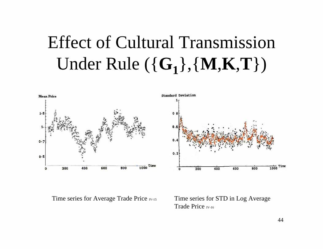
Effect of Cultural Transmission Under Rule ({G1},{M,K,T})
Time series for Average Trade Price IV-15 Time series for STD in Log Average Trade Price IV-16

45
Effect of Cultural Transmission (cont.)
• Emergent characteristics of note:– mean price is a random walk
– price variance is high. As an agent’s cultural preference (bias) changes, the effect is to change its metabolism for sugar and spice, moving it away from any price equilibrium it is tending toward.

46
Emergent Economic Networks
• Define a trade network as a graph:– agents are the nodes
– every trade, draw an edge between the agents
• Define a credit network as a graph:– created from the agent credit rule Ldr
– rule for borrowing and lending to have children
– forest of trees each rooted on a lender and ending on a borrower - internal nodes are both
47
For the Computer Scientist
• Abstract above the model– system with one or more attributes (resources)
– one or more parametrically distinct groups of individually heterogeneous agents
– simple rules of independent movement and attribute modification (resource gathering)
– simple rules of agent interaction (cultural transmission, trade)

48
For the Computer Scientist (cont.)
– genetic variation both horizontal between agents (cultural transmission) and vertical through generations (sexual reproduction)
• Applicability:– for developing systems manifesting large scale
patterns that correspond to emergent patterns discussed herein
– for operating on systems where these emergent properties may be effectively applied

49
That’s All Folks