Group descent algorithms for nonconvex penalized linear and

logistic regression models with grouped predictors

Patrick BrehenyDepartment of BiostatisticsUniversity of Kentucky

Jian HuangDepartment of Statistics

University of Iowa

March 15, 2013

Abstract

Penalized regression is an attractive framework for variable selection problems. Often, vari-ables possess a grouping structure, and the relevant selection problem is that of selecting groups,not individual variables. The group lasso has been proposed as a way of extending the ideas ofthe lasso to the problem of group selection. Nonconvex penalties such as SCAD and MCP havebeen proposed and shown to have several advantages over the lasso; these penalties may alsobe extended to the group selection problem, giving rise to group SCAD and group MCP meth-ods. Here, we describe algorithms for fitting these models stably and efficiently. In addition,we present simulation results and real data examples comparing and contrasting the statisticalproperties of these methods.

1 Introduction

In regression modeling, explanatory variables can often be thought of as grouped. To representa categorical variable, we may introduce a group of indicator functions. To allow flexible modelingof the effect of a continuous variable, we may introduce a series of basis functions. Or the variablesmay simply be grouped because the analyst considers them to be similar in some way, or because ascientific understanding of the problem implies that a group of covariates will have similar effects.

Taking this grouping information into account in the modeling process should improve both theinterpretability and the accuracy of the model. These gains are likely to be particularly importantin high-dimensional settings where sparsity and variable selection play important roles in estimationaccuracy.

Penalized likelihood methods for coefficient estimation and variable selection have becomewidespread since the original proposal of the lasso (Tibshirani, 1996). Building off of earlier workby Bakin (1999), Yuan and Lin (2006) extended the ideas of penalized regression to the prob-lem of grouped covariates. Rather than penalizing individual covariates, Yuan and Lin proposedpenalizing norms of groups of coefficients, and called their method the group lasso.

The group lasso, however, suffers from the same drawbacks as the lasso. Namely, it generallydoes not have the selection consistency property and tends to over-shrink large coefficients. Thisis because the rate of penalization of the group lasso does not change with the magnitude of thegroup coefficients, which leads to biased estimates of large coefficients. To compensate for theover-shrinkage, the group lasso tends to include spurious coefficients into the model.

1

The smoothly clipped absolute deviation (SCAD) penalty and the minimax concave penalty(MCP) were developed in an effort to achieve what the lasso could not: simultaneously selectionconsistency and asymptotic unbiasedness (Fan and Li, 2001; Zhang, 2010). This achievementis known as the oracle property, so named because it implies that the model is asymptoticallyequivalent to the fit of a maximum likelihood model in which the identities of the truly nonzerocoefficients are known in advance. These properties extend to group SCAD and group MCP models,as shown in Wang et al. (2008) and Huang et al. (2012).

However, group SCAD and group MCP have not been widely used or studied in comparison withthe group lasso, largely due to a lack of efficient and publicly available algorithms for fitting thesemodels. Published articles on the group SCAD (Wang et al., 2007, 2008) have used a local quadraticapproximation for fitting these models. The local quadratic approximation was originally proposedby Fan and Li (2001) to fit SCAD models. However, by relying on a quadratic approximation, theapproach is incapable of producing naturally sparse estimates, and therefore cannot take advantageof the computational benefits provided by sparsity. This, combined with the fact that solving thelocal quadratic approximation problem requires the repeated factorization of large matrices, makesthe algorithm very inefficient for fitting large regression problems. Zou and Li (2008) proposeda local linear approximation for fitting SCAD models and demonstrated its superior efficiency tolocal quadratic approximations. This algorithm was further improved upon by Breheny and Huang(2011), who demonstrated how a coordinate descent approach may used to fit SCAD and MCPmodels in a very efficient manner capable of scaling up to deal with very large problems.

Here, we show how the approach of Breheny and Huang (2011) may be extended to fit groupSCAD and group MCP models. We demonstrate that this algorithm is very fast and stable, and weprovide a publicly available implementation in the grpreg package (http://cran.r-project.org/web/packages/grpreg/index.html. In addition, we provide examples involving both simulatedand real data which demonstrate the potential advantages of group SCAD and group MCP overthe group lasso.

2 Group descent algorithms

We consider models in which the relationship between the outcome and the explanatory variablesis specified in terms of a linear predictor η:

η = β0 +J∑j=1

Xjβj , (2.1)

where Xj is the portion of the design matrix formed by the predictors in the jth group and the vectorβj consists of the associated regression coefficients. Letting Kj denote the number of members ingroup j, Xj is an n×Kj matrix with elements (xijk), the value of kth covariate in the jth groupfor the ith subject. Covariates that do not belong to any group may be thought of as a group ofone.

The problem of interest involves estimating a vector of coefficients β using a loss functionL which quantifies the discrepancy between yi and ηi combined with a penalty that encouragessparsity and prevents overfitting; specifically, we estimate β by minimizing

Q(β) = L(β|y,X) +J∑j=1

pλ(∥∥βj∥∥) , (2.2)

2

where p(·) is a penalty function applied to the Euclidean norm (L2 norm) of βj . The penalty isindexed by a regularization parameter λ, which controls the tradeoff between loss and penalty. Itis not necessary for λ to be the same for each group; i.e., we may consider a collection of regularityparameters {λj}. For example, in practice there are often variables known to be related to theoutcome and therefore which we do not wish to include in selection or penalization. The aboveframework and algorithms which follow may be easily extended to include such variables by settingλj = 0.

In this section, we primarily focus on linear regression, where E(y) = η and L is the leastsquares loss function, but take up the issue of logistic regression in Section 2.4, where L arises fromthe binomial likelihood. To ensure that the penalty is invariant to scale, covariates are standardizedprior to fitting such that

∑i xijk = 0 and n−1

∑i x

2ijk = 1. As emphasized in Simon and Tibshirani

(2011), this standardization is just as important for the group lasso as it is for the lasso, and is aseparate issue from that of orthogonalization (discussed in Section 2.1). We assume without lossof generality that the covariates are standardized in this way during the model fitting process andthen transformed back to the original scale once all models have been fit. For linear regression,we also assume, again without loss of generality, that the response has been centered such that∑

i yi = 0; in this case β0 = 0 and may be ignored.

2.1 Orthogonalization

The algorithm for fitting group lasso models originally proposed by Yuan and Lin (2006) requiresthe groups Xj to be orthonormal, as does the extension to logistic regression proposed in Meier et al.(2008). It is somewhat unclear from these papers, however, whether orthogonality is a necessaryaspect of problems that can be solved by the group lasso, or whether it may be introduced withoutloss of generality for the sake of model fitting.

We attempt to clarify the issue of orthonormality here, and demonstrate that groups may bemade orthonormal to aid in model fitting without any loss of generality, an issue is also discussed inSimon and Tibshirani (2011). This considerably extends the range of designs that can be analyzedwith the group lasso. For example, a group of indicator variables is orthonormal only under abalanced design having an equal number of observations in each category. Our approach requiresno such balance, however.

In this article, we develop algorithms dealing with the common scenario where the analyst (a)does not necessarily have orthogonal groups {Xj}, (b) wants solutions on the scale and units ofthe original explanatory variables, and (c) does not wish to deal with or think about any issues oforthonormality in fitting the model. In this section, we show that these goals may be accomplishedby orthogonalizing Xj using a singular value decomposition, fitting the model, and then using thedecomposition to transform the solution back to the original scale.

Taking the singular value decomposition of the Gram matrix of the jth group, we have

1

nXTj Xj = QjΛjQ

Tj ,

where Λj is a diagonal matrix containing the eigenvalues of n−1XTj Xj and Qj is an orthonormal

matrix of its eigenvectors. Now, we may construct a linear transformation Xj = XjQjΛ−1/2j with

3

the following properties:

1

nXTj Xj = I (2.3)

Xjβj = Xj(QjΛ−1/2j βj), (2.4)

where I is the identity matrix and βj is the solution to (2.2) on the orthogonalized scale. Inother words, if we have the solution to the orthogonalized problem, we may easily transform back

to the original problem with βj = QjΛ−1/2j βj . This procedure is not terribly expensive from a

computational standpoint, as the decompositions are being applied only to the groups, not theentire design matrix, and the inverses are of course trivial to compute because ΛJ is diagonal.Furthermore, the decompositions need only be computed once initially, not with every iteration.

Note that this procedure may be applied even when Xj is not full-rank by omitting the zeroeigenvalues and their associated eigenvectors. In this case, Qj is a Kj × rj matrix and Λ is anrj × rj matrix, where rj denotes the rank of Xj . Given these modifications, Λ is invertible and

Xj = XjQjΛ−1/2j still possesses properties (2.3) and (2.4). Note, however, that Xj now contains

only rj columns and by extension, βj contains only rj elements. Thus, we avoid the problem ofincomplete rank by fitting the model in a lower-dimensional parameter space, then transformingback to the original dimensions (note that applying the reverse transformation results in a βjwith appropriate dimension Kj). In the special case where two members of a group are identical,xjk = xj`, this approach ensures that their coefficients, βjk and βj`, will be equal for all values ofλ.

For the remainder of this article, we will assume that this process has been applied and thatthe model fitting algorithms we describe are being applied to orthogonal groups, and we will dropthe tildes on X and β in the rest of the article. It is worth clarifying that by “orthogonal groups”,we mean groups for which n−1XT

j Xj = I, not that groups Xj and Xk are orthogonal to each other.Again, we note that this orthonormalization may be accomplished without loss of generality:

we are still solving the original minimization problem, simply with a change of variables to aid inthe model fitting process. Furthermore, the issue of orthogonalization is entirely separate from theissue of standardization (requiring that n−1

∑i x

2ijk = 1). Both standardized and unstandardized

groups Xj may be orthogonalized with the approach described above. Unlike orthonormalization,standardization does change the minimization problem and results in different estimates of β.However, the standardized solution, being equivariant to changes of scale, is preferred.

2.2 Group lasso

In this section, we describe the group lasso and algorithms for fitting group lasso models. Thegroup lasso estimator, originally proposed by Yuan and Lin (2006), is defined as the value β thatminimizes

Q(β) =1

2n‖y −Xβ‖2 + λ

∑j

√Kj

∥∥βj∥∥ . (2.5)

The idea behind the penalty is to apply a lasso penalty to the Euclidean (L2) norm of each group,thereby encouraging sparsity and variable selection at the group level. The solution β has theproperty that if group j is selected, then βjk 6= 0 for all k, otherwise βjk = 0 for all k. The

4

β1

β 2

0.0 0.5 1.0 1.5

0.0

0.5

1.0

1.5

β1

β 2

0.0 0.5 1.0 1.5

0.0

0.5

1.0

1.5

Figure 1: The impact of orthogonalization on the solution to the group lasso. Contour lines forthe likelihood (least squares) surface are drawn, centered around the OLS solution, as well as thesolution path for the group lasso as λ goes from 0 to∞. Left: Non-orthogonal X. Right: OrthogonalX.

magnitude of∥∥βj∥∥ will tend to be larger if βj has more elements; the presence of the

√Kj term

counteracts this tendency, thereby normalizing for group size. As discussed in Simon and Tibshirani(2011), this results in variable selection which is roughly equivalent to the uniformly most powerfulinvariant test for inclusion of the jth group. In what follows, we will absorb the

√Kj term into λ

and use λj = λ√Kj .

Yuan and Lin (2006) also propose an algorithm which they base on the “shooting algorithm”of Fu (1998). Here, we refer to this type of algorithm as a “group descent” algorithm. The ideabehind the algorithm is the same as that of coordinate descent algorithms (Friedman et al., 2007;Wu and Lange, 2008), with the modification that the optimization of (2.5) takes place repeatedlywith respect to a group βj rather than an individual coordinate βj .

Below, we present the group descent algorithm for solving (2.5) to obtain the group lassoestimator. The algorithm is essentially the same as Yuan and Lin’s, although (a) we have generalizedit to the case of non-orthogonal groups using the approach described in Section 2.1, (b) we restatethe algorithm to more clearly illustrate the connections with coordinate descent algorithms, and (c)we employ techniques developed in the coordinate descent literature to speed up the implementationof the algorithm considerably. As we will see, this presentation of the algorithm also makes clearhow to easily extend it to fit group SCAD and group MCP models in the following sections.

We begin by noting that the subdifferential (Bertsekas, 1999) of Q with respect to βj is givenby

∂Q(βj) = −zj + βj + λjsβj/∥∥βj∥∥ , (2.6)

where zj = XTj (y−X−jβ−j) is the least squares solution, X−j is the portion of the design matrix

that remains after Xj has been excluded, β−j are its associated regression coefficients, and s = 1for βj 6= 0 and s ∈ [−1, 1] otherwise. The main implication of (2.6) is that, by orthogonalizing the

5

groups, Xj drops out of the equation and the multivariate problem of optimizing with respect toβj is reduced to a univariate problem, as the solution must lie on the line segment joining 0 and zj .The geometry of this problem is illustrated in Figure 1. As the figure illustrates, orthogonalizationrenders the direction of βj invariant with respect to λ, thereby enabling us to break the solutiondown into two components: determining the direction of βj and determining its length.

Furthermore, determining the length of βj is equivalent to solving a one-dimensional lassoproblem, which has a simple, closed-form solution given by the soft-thresholding operator (Donohoand Johnstone, 1994):

S(z, λ) =

z − λ if z > λ

0 if |z| ≤ λz + λ if z < −λ.

(2.7)

With a slight abuse of notation, we extend this definition to a vector-valued argument z as follows:

S(z, λ) = S(‖z‖ , λ)z

‖z‖, (2.8)

where z/ ‖z‖ is the unit vector in the direction of z. In other words, S(z, λ) acts on a vector z byshortening it towards 0 by an amount λ, and if the length of z is less than λ, the vector is shortenedall the way to 0.

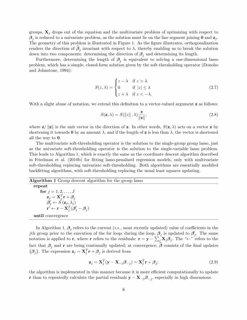
The multivariate soft-thresholding operator is the solution to the single-group group lasso, justas the univariate soft-thresholding operator is the solution to the single-variable lasso problem.This leads to Algorithm 1, which is exactly the same as the coordinate descent algorithm describedin Friedman et al. (2010b) for fitting lasso-penalized regression models, only with multivariatesoft-thresholding replacing univariate soft-thresholding. Both algorithms are essentially modifiedbackfitting algorithms, with soft-thresholding replacing the usual least squares updating.

Algorithm 1 Group descent algorithm for the group lassorepeat

for j = 1, 2, . . . , Jzj = XT

j r + βjβ′j ← S (zj , λj)

r′ ← r−XTj (β′j − βj)

until convergence

In Algorithm 1, βj refers to the current (i.e., most recently updated) value of coefficients in thejth group prior to the execution of the for loop; during the loop, βj is updated to β′j . The samenotation is applied to r, where r refers to the residuals: r = y −

∑j Xjβj . The “←” refers to the

fact that βj and r are being continually updated; at convergence, β consists of the final updates

{βj}. The expression zj = XTj r + βj is derived from

zj = XTj (y −X−jβ−j) = XT

j r + βj ; (2.9)

the algorithm is implemented in this manner because it is more efficient computationally to updater than to repeatedly calculate the partial residuals y −X−jβ−j , especially in high dimensions.

6

The computational efficiency of Algorithm 1 is clear: no complicated numerical optimizationsteps or matrix factorizations or inversions are required, only a small number of simple arithmeticoperations. This efficiency is possible only because the groups {Xj} are made to be orthogonal priorto model fitting. Without this initial orthogonalization, we cannot obtain the simple closed-formsolution (2.8), and the updating steps required to fit the group lasso become considerably morecomplicated, as in Friedman et al. (2010a) and Foygel and Drton (2010).

2.3 Group MCP and group SCAD

We have just seen how the group lasso may be viewed as applying the lasso/soft-thresholdingoperator to the length of each group. Not only does this formulation lead to a very efficientalgorithm, it also makes it clear how to extend other univariate penalties to the group setting.Here, we focus on two popular alternative univariate penalties to the lasso: SCAD, the smoothlyclipped absolute deviation penalty (Fan and Li, 2001) and MCP, the minimax concave penalty(Zhang, 2010).

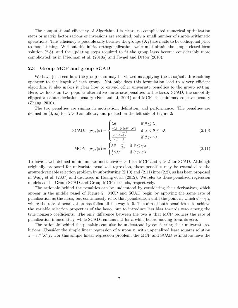
The two penalties are similar in motivation, definition, and performance. The penalties aredefined on [0,∞) for λ > 0 as follows, and plotted on the left side of Figure 2:

SCAD: pλ,γ(θ) =

λθ if θ ≤ λγλθ−0.5(θ2+λ2)

γ−1 if λ < θ ≤ γλλ2(γ2−1)2(γ−1) if θ > γλ

(2.10)

MCP: pλ,γ(θ) =

{λθ − θ2

2γ if θ ≤ γλ12γλ

2 if θ > γλ. (2.11)

To have a well-defined minimum, we must have γ > 1 for MCP and γ > 2 for SCAD. Althoughoriginally proposed for univariate penalized regression, these penalties may be extended to thegrouped-variable selection problem by substituting (2.10) and (2.11) into (2.2), as has been proposedin Wang et al. (2007) and discussed in Huang et al. (2012). We refer to these penalized regressionmodels as the Group SCAD and Group MCP methods, respectively.

The rationale behind the penalties can be understood by considering their derivatives, whichappear in the middle panel of Figure 2. MCP and SCAD begin by applying the same rate ofpenalization as the lasso, but continuously relax that penalization until the point at which θ = γλ,where the rate of penalization has fallen all the way to 0. The aim of both penalties is to achievethe variable selection properties of the lasso, but to introduce less bias towards zero among thetrue nonzero coefficients. The only difference between the two is that MCP reduces the rate ofpenalization immediately, while SCAD remains flat for a while before moving towards zero.

The rationale behind the penalties can also be understood by considering their univariate so-lutions. Consider the simple linear regression of y upon x, with unpenalized least squares solutionz = n−1xTy. For this simple linear regression problem, the MCP and SCAD estimators have the

7

θ

0

λ

− γλ − λ 0 λ γλ

Lasso

SCAD

MCP

p(θ)

θ

0

λ

0 λ γλ

Lasso

SCAD

MCP

p′(θ)

z

0λ

− γλ − λ 0 λ γλ

Lasso

SCAD

MCP

Solution

Figure 2: Lasso, SCAD, and MCP penalty functions, derivatives, and univariate solutions. Thepanel on the left plots the penalties themselves, the middle panel plots the first derivative ofthe penalty, and the right panel plots the univariate solutions as a function of the ordinary leastsquares estimate. The light gray line in the rightmost plot is the identity line. Note that none ofthe penalties are differentiable at βj = 0.

following closed forms:

β = F (z, λ, γ) =

{S(z,λ)1−1/γ if |z| ≤ γλz if |z| > γλ,

(2.12)

β = FS(z, λ, γ) =

S(z, λ) if |z| ≤ 2λS(z,γλ/(γ−1))1−1/(γ−1) if 2λ < |z| ≤ γλ

z if |z| > γλ.

(2.13)

Noting that S(z, λ) is the univariate solution to the lasso, we can observe by comparison that MCPand SCAD scale the lasso solution upwards toward the unpenalized solution by an amount thatdepends on γ. For both MCP and SCAD, when |z| > γλ, the solution is scaled up fully to theunpenalized least squares solution. These solutions are plotted in the right panel of Figure 2; thefigure illustrates how the solutions, as a function of z, make a smooth transition between the lassoand least squares solutions. This transition is essential to the oracle property described in theintroduction.

As γ → ∞, the MCP and lasso solutions are identical. As γ → 1, the MCP solution becomesthe hard thresholding estimate zI|z|>λ. Thus, in the univariate sense, the MCP produces the “firmshrinkage” estimator of Gao and Bruce (1997); hence the F (·) notation. The SCAD solutionsare similar, of course, but not identical, and thus involve a “SCAD-modified firm thresholding”operator which we denote FS(·). In particular, the SCAD solutions also have soft-thresholding asthe limiting case when γ →∞, but do not have hard thresholding as the limiting case when γ → 2.

We extend these two firm-thresholding operators to multivariate arguments as in (2.8), with F (·)or FS(·) taking the place of S(·), and note that F (zj , λ, γ) and FS(zj , λ, γ) optimize the objectivefunctions for Group MCP and Group SCAD, respectively, with respect to βj . An illustration ofthe nature of these estimators is given in Figure 3. We note the following: (1) All estimators carryout group selection, in the sense that, for any value of λ, the coefficients belonging to a group areeither wholly included or wholly excluded from the model. (2) The group MCP and group SCAD

8

1.4 1.2 1.0 0.8 0.6 0.4 0.2 0.0

−0.5

0.0

0.5

1.0

Group lasso

λ

β A B C

1.4 1.2 1.0 0.8 0.6 0.4 0.2 0.0

−0.5

0.0

0.5

1.0

Group MCP

λ

β A B C

1.4 1.2 1.0 0.8 0.6 0.4 0.2 0.0

−0.5

0.0

0.5

1.0

Group SCAD

λ

β A B C

Figure 3: Representative solution paths for the group lasso, group MCP, and group SCAD methods.In the generating model, groups A and B have nonzero coefficients and while those belonging togroup C are zero.

methods eliminate some of the bias towards zero introduced by the group lasso. In particular, atλ ≈ 0.2, they produce the same estimates as a least squares regression model including only thenonzero covariates (the “oracle” model). (3) Group MCP makes a smoother transition from 0 tothe unpenalized solutions than group SCAD. This is the “minimax” aspect of the penalty. Anyother penalty that makes the transition between these two extremes must have some region (e.g.λ ∈ [0.7, 0.5] for group SCAD) in which its solutions are changing more abruptly than those ofgroup MCP.

It is straightforward to extend Algorithm 1 to fit Group SCAD and Group MCP models; allthat is needed is to replace the multivariate soft-thresholding update with a multivariate firm-thresholding update. The group updates for all three methods are listed below:

Group lasso : βj ← S(zj , λ) = S(‖zj‖ , λ)zj‖zj‖

Group MCP : βj ← F (zj , λ, γ) = F (‖zj‖ , λ, γ)zj‖zj‖

Group SCAD : βj ← F (zj , λ, γ) = FS(‖zj‖ , λ, γ)zj‖zj‖

Note that all three updates are simple, closed-form expressions. Furthermore, as each updateminimizes the objective function with respect to βj , the algorithms possess the descent property,meaning that they decrease the objective function with every iteration and are therefore guaranteedto converge, a fact which we now state formally.

Proposition 1. Let β(m) denote the value of the fitted regression coefficient at the end of iterationm. At every iteration of the proposed group descent algorithms for linear regression models involvinggroup lasso, group MCP, or group SCAD penalties,

Q(β(m+1)) ≤ Q(β(m)).

Furthermore, the sequence {β(1),β(2), . . .} is guaranteed to converge to a stationary point of Q.

9

For the group lasso penalty, the objective function being minimized is convex, and thus theabove proposition establishes convergence to the global minimum. For group MCP and groupSCAD, whose objective function is a sum of convex and nonconvex components, convergence to alocal minimum is possible.

It is worth pointing out that a similar algorithm was explored in She (2012), who proposedthe same updating steps as above, although without an initial orthogonalization. Interestingly,She showed that even without orthogonalization, the updating steps still produce a sequence β(m)

converging to a stationary point of the objective function. Unlike our approach, however, theseupdates are not exact group-wise solutions. In other words, in the single-group case, our approachproduces exact solutions in one step, whereas the approach in She (2012) requires multiple iterationsto converge to the same solution. This leads to a considerable loss of efficiency, as we will see inSection 3.

In conclusion, the algorithms we present here for fitting group lasso, group MCP, and groupSCAD models are both fast and stable. We examine the empirical running time of these algorithmsin Section 3.

2.4 Logistic regression

It is possible to extend the algorithms described above to fit group-penalized logistic regressionmodels as well, where the loss function is the negative log-likelihood of a binomial distribution:

L(η) =1

n

∑i

Li(ηi) = − 1

n

∑i

logP(yi|ηi).

Recall, however, that the simple, closed form solutions of the previous sections were possible onlywith orthogonalization. The iteratively reweighted least squares (IRLS) algorithm typically used tofit generalized linear models (GLMs) introduces a n−1XTWX term into the score equation (2.6),where W is an n× n diagonal matrix of weights. Because n−1XTWX 6= I, the group lasso, groupMCP, and group SCAD solutions will lack the simple closed forms of the previous section.

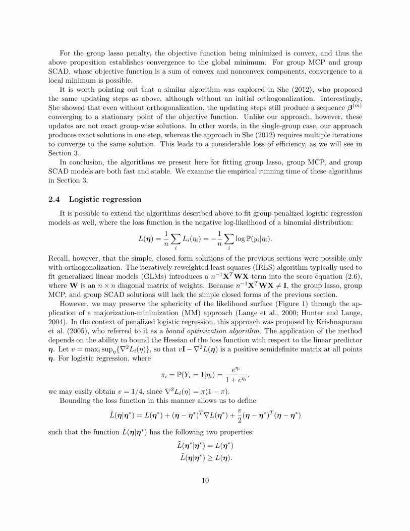
However, we may preserve the sphericity of the likelihood surface (Figure 1) through the ap-plication of a majorization-minimization (MM) approach (Lange et al., 2000; Hunter and Lange,2004). In the context of penalized logistic regression, this approach was proposed by Krishnapuramet al. (2005), who referred to it as a bound optimization algorithm. The application of the methoddepends on the ability to bound the Hessian of the loss function with respect to the linear predictorη. Let v = maxi supη{∇2Li(η)}, so that vI−∇2L(η) is a positive semidefinite matrix at all pointsη. For logistic regression, where

πi = P(Yi = 1|ηi) =eηi

1 + eηi,

we may easily obtain v = 1/4, since ∇2Li(η) = π(1− π).Bounding the loss function in this manner allows us to define

L(η|η∗) = L(η∗) + (η − η∗)T∇L(η∗) +v

2(η − η∗)T (η − η∗)

such that the function L(η|η∗) has the following two properties:

L(η∗|η∗) = L(η∗)

L(η|η∗) ≥ L(η).

10

Thus, L(η|η∗) is a majorizing function of L(η). The theory underlying MM algorithms then ensuresthat Algorithm 2, which consists of alternately executing the majorizing step and the minimizationsteps, will retain the descent property of the previous sections, which we formally state below.

Proposition 2. Let β(m) denote the value of the fitted regression coefficient at the end of iterationm. At every iteration of the proposed group descent algorithms for logistic regression involvinggroup lasso, group MCP, or group SCAD penalties,

Q(β(m+1)) ≤ Q(β(m)).

Furthermore, provided that no elements of β tend to ±∞, the sequence {β(1),β(2), . . .} is guaranteedto converge to a stationary point of Q.

As with linear regression, this result implies convergence to a global minimum for the grouplasso, but allows convergence to local minima for group MCP and group SCAD. Note, however, thatunlike linear regression, in logistic regression maximum likelihood estimates can occur at ±∞ (thisis often referred to as complete separation). In practice, this is not a concern for large values of λ,but saturation of the model will certainly occur when p > n and λ is small. Our implementation ingrpreg terminates the path-fitting algorithm if saturation is detected, based on a check of whether> 99% of the null deviance has been explained by the model.

Writing L(η|η∗) in terms of β, we have

L(β) ∝ v

2n(y −Xβ)T (y −Xβ),

where y = η∗+(y−π)/v is the pseudo-response vector. Thus, the gradient of L(η|η∗) with respectto βj is given by

∇L(βj) = −vzj + vβj , (2.14)

where, as before, zj = XTj (y −X−jβ−j) is the vector of partial (pseudo-) residuals for βj .

Algorithm 2 Group descent algorithm for logistic regression with a group lasso penaltyrepeat

η ← Xβπ ← {eηi/(1 + eηi)}ni=1

r← (y − π)/vfor j = 1, 2, . . . , J

zj = XTj r + βj

β′j ← S (vzj , λj) /v

r′ ← r−XTj (β′j − βj)

until convergence

The presence of the scalar v in the score equations affects the updating equations; however, asthe majorized loss function remains spherical with respect to β, the updating equations still have

11

simple, closed form solutions:

Group lasso : βj ←1

vS(vzj , λ) =

1

vS(v ‖zj‖ , λ)

zj‖zj‖

Group MCP : βj ←1

vF (vzj , λ, γ) =

1

vF (v ‖zj‖ , λ, γ)

zj‖zj‖

Group SCAD : βj ←1

vF (vzj , λ, γ) =

1

vFS(v ‖zj‖ , λ, γ)

zj‖zj‖

Algorithm 2 is presented for the group lasso, but is easily modified to fit group MCP and groupSCAD models by substituting the appropriate expression into the updating step for βj .

Note that Proposition 2 does not necessarily follow for other generalized linear models, as theHessian matrices for other exponential families are typically unbounded. One possibility is to setv ← maxi{∇2Li(η

∗i )} at the beginning of each iteration as a pseudo-upper bound. As this is not

an actual upper bound, an algorithm based on it is not guaranteed to possess the descent property.Still, this approach would seem likely to provide adequate performance in practice, although theauthors have not examined the proposal in depth.

2.5 Path-fitting algorithm

The above algorithms are presented from the perspective of fitting a penalized regression modelfor a single value of λ. Usually, we are interested in obtaining β for a range of λ values, and thenchoosing among those models using either cross-validation or some form of information criterion.The regularization parameter λ may vary from a maximum value λmax at which all penalizedcoefficients are 0 down to λ = 0 or to a minimum value λmin beyond which the model becomesexcessively large. When the objective function is strictly convex, the estimated coefficients varycontinuously with λ ∈ [λmin, λmax] and produce a path of solutions regularized by λ. An examplesof such a path may be seen in Figure 3.

Algorithms 1 and 2 are iterative and require initial values; the fact that β = 0 at λmax providesan efficient approach to choosing those initial values. Group lasso, group MCP, and group SCADall have the same value of λmax; namely, λmax = maxj{‖zj‖} for linear regression or λmax =maxj{v ‖zj‖} for logistic regression, where the {zj} are computed with respect to the intercept-only model (or, if unpenalized covariates are present, with respect to the residuals of the fittedmodel including all of the unpenalized covariates). Thus, by starting at λmax where β = 0 isavailable in closed form and proceeding towards λmin, using β from the previous value of λ as theinitial value for the next value of λ, we can ensure that the initial values will never be far from thesolution, a helpful property often referred to as “warm starts” in the path-fitting literature.

3 Algorithm efficiency

Here, we briefly comment on the efficiency of the proposed algorithms. Regardless of the penaltychosen, the most computationally intensive steps in Algorithm 1 are the calculation of the innerproducts XT

j r and XTj (β′j − βj), each of which requires O(nKj) operations. Thus, one full pass

over all the groups requires O(2np) operations. The fact that this approach scales linearly in pallows it to be efficiently applied to high-dimensional problems.

12

Table 1: Comparison of (grpreg) with other publicly available group lasso packages. Times arein seconds required to fit the entire solution path over a grid of 100 λ values, averaged over 100independent data sets. Each group consisted of 10 variables; thus p ranges over {10, 100, 1000}across the columns.

n=50 n=500 n=5000J=1 J=10 J=100

Linear grpreg Group lasso 0.01 0.07 18.42regression grpreg Group MCP 0.01 0.05 10.66

grpreg Group SCAD 0.01 0.05 11.04grplasso Group lasso 0.16 1.91 60.96standGL Group lasso 0.04 1.27 150.99

Logistic grpreg Group lasso 0.01 0.21 107.90regression grpreg Group MCP 0.01 0.13 46.26

grpreg Group SCAD 0.01 0.14 83.08grplasso Group lasso 1.20 5.15 203.22standGL Group lasso 0.43 6.40 399.42

Of course, the entire time required to fit the model depends on the number of iterations, whichin turn depends on the data and on λ. Broadly speaking, the dominant factor influencing thenumber of iterations is the number of nonzero groups at that value of λ, since no iteration isrequired to solve for groups that remain fixed at zero. Consequently, when fitting a regularizedpath, a disproportionate amount of time is spent at the least sparse end of the path, where λ issmall.

Table 1 compares our implementation (grpreg) with two other publicly available R packagesfor fitting group lasso models over increasingly large data sets: the grplasso package (Meieret al., 2008) and the standGL package (Simon and Tibshirani, 2011). We note that (a) the grpreg

implementation appears uniformly more efficient than the others, and (b) that group MCP andgroup SCAD tend to be slightly faster than group lasso. Presumably, this is caused by the factthat their solution paths tend to be more sparse.

It is worth noting that all three of these packages can handle p > n problems; however, for thepurposes of timing, we chose to restrict our attention to problems in which the entire path canbe computed. Otherwise, different implementations may terminate the fitting process at differentpoints along the path, which would prevent a fair comparison of computing times.

Finally, let us compare these results to those presented in She (2012). For the algorithmpresented in that paper, the author reports an average time of 32 minutes to estimate the groupSCAD regression coefficients when n = 100 and p = 500. For the same size problem, our approachrequired a mere 0.35 seconds.

4 Simulation studies

In this section, we compare the performance of group lasso, group MCP, and group SCADusing simulated data. First, a relatively basic setting is used to illustrate the primary advantages

13

of group MCP and group SCAD over group lasso. We then attempt to mimic two settings in whichthe methodology might be used: to allow flexible semiparametric modeling of continuous variablesand in genetic association studies, which involve large numbers of categorical variables. We use theterm “null predictor” to refer to a covariate whose associated regression coefficient is zero in thetrue model.

In all of the studies, five-fold cross-validation was used to choose the regularization parameterλ. Group SCAD and group MCP have an additional tuning parameter, γ. In principle, one mayattempt to select optimal values of γ using, for example, cross-validation over a two-dimensionalgrid or using an information criterion approach. Here, we fix γ = 3 for group MCP and γ = 4 forgroup SCAD, roughly in line with the default recommendations suggested in Fan and Li (2001)and Zhang (2010) in the non-grouped case.

In Section 4.1, we evaluate model accuracy by root mean squared error (RMSE):

RMSE =

√1

p

∑j,k

(βjk − βjk)2.

In Sections 4.2 and 4.3, because the model fit to the data is not always the same as the generatingmodel, we focus on root model error (RME) instead:

RME =

√1

n

∑i

(µi − µi)2,

where µi and µi denote the true and estimated mean of observation i given xi. Note that the modelerror, which is also discussed in Fan and Li (2001), is equal in expected value to the prediction errorminus the irreducible error σ2. In all simulations, results are averaged over 1,000 independentlygenerated data sets.

4.1 Basic

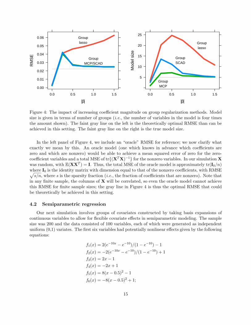
We begin with a very straightforward study designed to illustrate the basic shortcomings of thegroup lasso in comparison with group MCP and group SCAD. The design matrix consists of 100groups, each with 4 elements. In five of these groups, the coefficients are ±β; in the others, thetrue regression coefficients are zero. Covariate values and errors were generated from the standardnormal distribution. We fixed the sample size at 100 (i.e., n=100, p=400) and varied |β|. Inprinciple, group lasso should struggle when |β| is large, as it cannot alleviate the problem of biastowards zero for large coefficients without lowering λ and thereby allowing null predictors to enterthe model. Indeed, as Figure 4 illustrates, this is exactly what occurs.

For small values of the regression coefficients, all three group regularization methods performsimilarly. As we increase the magnitude of these coefficients, however, group MCP and groupSCAD begin to estimate β with an error approaching the theoretically optimal value, while grouplasso performs increasingly poorly. Furthermore, group MCP and group SCAD select much smallermodels and approach the true model size much faster than group lasso, which selects far too manyvariables.

Comparing group MCP and group SCAD, the two are nearly identical in terms of estimationaccuracy. However, group MCP selects a considerably more sparse model, and has better variableselection properties. Thus, although the two methods behave similarly in an asymptotic setting,group MCP seems to have somewhat better finite-sample properties.

14

β

RM

SE

0.00

0.01

0.02

0.03

0.04

0.05

0.06

0.0 0.5 1.0 1.5

Grouplasso

GroupMCP/SCAD

β

Mod

el s

ize

5

10

15

20

25

0.0 0.5 1.0 1.5

Grouplasso

GroupSCAD

GroupMCP

Figure 4: The impact of increasing coefficient magnitude on group regularization methods. Modelsize is given in terms of number of groups (i.e., the number of variables in the model is four timesthe amount shown). The faint gray line on the left is the theoretically optimal RMSE than can beachieved in this setting. The faint gray line on the right is the true model size.

In the left panel of Figure 4, we include an “oracle” RMSE for reference; we now clarify whatexactly we mean by this. An oracle model (one which knows in advance which coefficients arezero and which are nonzero) would be able to achieve a mean squared error of zero for the zero-coefficient variables and a total MSE of tr{(XTX)−1} for the nonzero variables. In our simulation Xwas random, with E(XXT ) = I. Thus, the total MSE of the oracle model is approximately tr(I0/n)where I0 is the identity matrix with dimension equal to that of the nonzero coefficients, with RMSE√s/n, where s is the sparsity fraction (i.e., the fraction of coefficients that are nonzero). Note that

in any finite sample, the columns of X will be correlated, so even the oracle model cannot achievethis RMSE for finite sample sizes; the gray line in Figure 4 is thus the optimal RMSE that couldbe theoretically be achieved in this setting.

4.2 Semiparametric regression

Our next simulation involves groups of covariates constructed by taking basis expansions ofcontinuous variables to allow for flexible covariate effects in semiparametric modeling. The samplesize was 200 and the data consisted of 100 variables, each of which were generated as independentuniform (0,1) variates. The first six variables had potentially nonlinear effects given by the followingequations:

f1(x) = 2(e−10x − e−10)/(1− e−10)− 1

f2(x) = −2(e−10x − e−10)/(1− e−10) + 1

f3(x) = 2x− 1

f4(x) = −2x+ 1

f5(x) = 8(x− 0.5)2 − 1

f6(x) = −8(x− 0.5)2 + 1;

15

the other 94 had no effect on the outcome. The scaling of the functions is to ensure that eachvariable attains a minimum and maximum of (−1, 1) over the domain of x and thus that theeffects of all six variables are roughly comparable. Visually the effect of the six nonzero variablesis illustrated below:

x1 x2 x3 x4 x5 x6

For model fitting, each variable was represented using a 6-term B-spline basis expansion (i.e., Xhad dimensions n = 200, p = 600). In addition to the three group selection methods, models werealso fit using the lasso (i.e., ignoring grouping). Results are given in Table 2.

Table 2: Prediction and variable selection accuracy for the semiparametric regression simulation.

Group Group GroupLasso Lasso MCP SCAD

RME 0.73 0.59 0.50 0.52Variables selected 31.5 29.3 10.4 23.1

Certainly, all three group selection approaches greatly outperform the lasso here. However, as inthe previous section, group MCP and group SCAD are able to achieve superior prediction accuracywhich selecting more parsimonious models. Also as in the previous simulation, group MCP andgroup SCAD perform similarly as far as prediction accuracy, but group MCP is seen to have betterfinite-sample variable selection properties — recall that the true number of variables in the modelis only 6.

4.3 Genetic association study

Finally, we carry out a simulation designed to mimic a small genetic association study involvingsingle nucleotide polymorphisms (SNPs). Briefly, a SNP is a point on the genome in which multipleversions (alleles) may be present. A SNP may take on three values {0, 1, 2}, depending on thenumber of minor alleles present. The effect is not necessarily linear — for example, if the allele hasa recessive effect, the phenotype associated with x = 0 and x = 1 are identical, while the phenotypeassociated with x = 2 is different. In such studies, it is desirable to have a method which is robustto different mechanisms of action, yet powerful enough to actually detect important SNPs, as thenumber of SNPs is typically rather large.

We simulated data involving 250 subjects and 500 SNPs, each of which was represented with 2indicator functions (i.e., n=250, p=1,000). Three of the variables had an effect on the phenotype(one dominant effect, one recessive effect, one additive effect); the other 497 did not. In additionto the three group selection methods, we included for comparison two versions of the lasso: oneapplied to all p = 1, 000 variables and ignoring grouping, the other assuming an additive effect foreach genotype. Note that for the second approach, p = 500 as we estimate only a single coefficientfor each SNP. The results of this simulation are given in Table 3.

16

Table 3: Prediction and variable selection accuracy for the genetic association study simulation.True discoveries are selected variables that have a truly nonzero effect; false discoveries are selectedSNPs that have no effect on the phenotype.

Additive Group Group GroupLasso Lasso Lasso MCP SCAD

RME 0.38 0.37 0.34 0.25 0.27True discoveries 2.6 2.2 2.6 2.4 2.5False discoveries 21.1 16.3 15.5 4.0 12.5

The same broad conclusions may be reached here as in the previous simulations. In particular,we note that (1) The group selection methods outperform the variable selection methods thateither do not account for grouping or that attempt to incorporate grouping in an ad-hoc fashion.(2) Group MCP and group SCAD outperform the group lasso both in terms of prediction accuracyas well as the number of false discoveries. (3) Although group MCP and group SCAD are similarin terms of prediction accuracy, group MCP has significantly better variable selection properties,producing only four false discoveries compared to group SCAD’s 12.5.

5 Real data

We give two examples of applying grouped variable selection methods to real data. The firstis a gene expression study in rats to determine genes associated with Bardet-Biedl syndrome.The second is a genetic association study to determine SNPs associated with age-related maculardegeneration. As in the previous section, we fix γ = 3 for group MCP, γ = 4 for group SCAD, andselect λ via cross-validation.

5.1 Bardet-Biedl syndrome gene expression study

The data we analyze here is discussed more fully in Scheetz et al. (2006). Briefly, the dataset consists of normalized microarray gene expression data harvested from the eye tissue of 120twelve-week-old male rats. The outcome of interest is the expression of TRIM32, a gene whichhas been shown to cause Bardet-Biedl syndrome (Chiang et al., 2006). Bardet-Biedl syndrome is agenetic disease of multiple organ systems including the retina.

Following the approach in Scheetz et al. (2006), 18,976 of the 31,042 probe sets on the array“exhibited sufficient signal for reliable analysis and at least 2-fold variation in expression.” Theseprobe sets include TRIM32 and 18,975 other genes that potentially influence its expression. Wefurther restricted our attention to the 5,000 genes with the largest variances in expression (on thelog scale) and considered a three-term natural cubic spline basis expansion of those genes, resultingin a grouped regression problem with n = 120 and p = 15, 000. The models selected by group lasso,group MCP, and group SCAD are described in Table 4.

This is an interesting case study in that group MCP selects a very different model from theother two approaches. In particular, group lasso and group SCAD each select a fairly large numberof genes, while shrinking each gene’s group of coefficients nearly to zero. Group MCP, on the otherhand, selects a single gene and returns a fit nearly the same as the least-squares fit for that gene

17

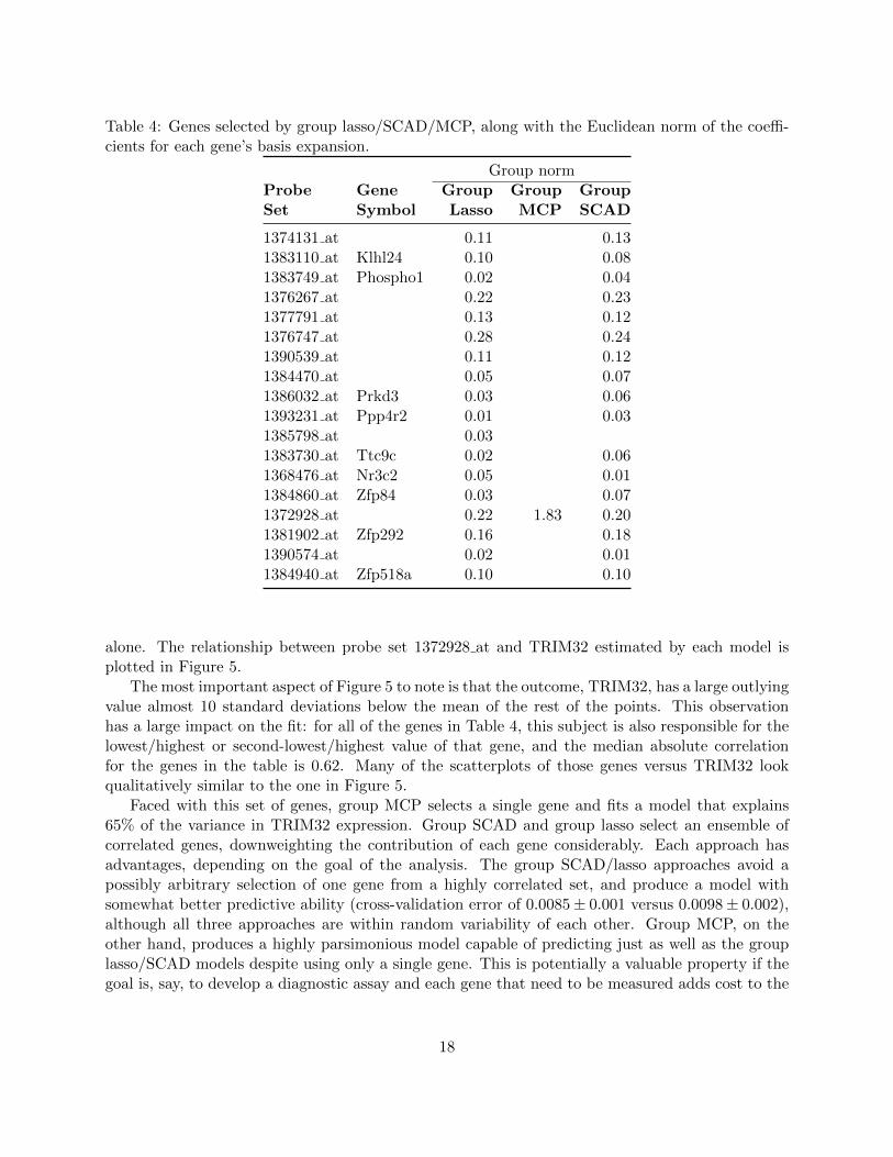
Table 4: Genes selected by group lasso/SCAD/MCP, along with the Euclidean norm of the coeffi-cients for each gene’s basis expansion.

Group normProbe Gene Group Group GroupSet Symbol Lasso MCP SCAD

1374131 at 0.11 0.131383110 at Klhl24 0.10 0.081383749 at Phospho1 0.02 0.041376267 at 0.22 0.231377791 at 0.13 0.121376747 at 0.28 0.241390539 at 0.11 0.121384470 at 0.05 0.071386032 at Prkd3 0.03 0.061393231 at Ppp4r2 0.01 0.031385798 at 0.031383730 at Ttc9c 0.02 0.061368476 at Nr3c2 0.05 0.011384860 at Zfp84 0.03 0.071372928 at 0.22 1.83 0.201381902 at Zfp292 0.16 0.181390574 at 0.02 0.011384940 at Zfp518a 0.10 0.10

alone. The relationship between probe set 1372928 at and TRIM32 estimated by each model isplotted in Figure 5.

The most important aspect of Figure 5 to note is that the outcome, TRIM32, has a large outlyingvalue almost 10 standard deviations below the mean of the rest of the points. This observationhas a large impact on the fit: for all of the genes in Table 4, this subject is also responsible for thelowest/highest or second-lowest/highest value of that gene, and the median absolute correlationfor the genes in the table is 0.62. Many of the scatterplots of those genes versus TRIM32 lookqualitatively similar to the one in Figure 5.

Faced with this set of genes, group MCP selects a single gene and fits a model that explains65% of the variance in TRIM32 expression. Group SCAD and group lasso select an ensemble ofcorrelated genes, downweighting the contribution of each gene considerably. Each approach hasadvantages, depending on the goal of the analysis. The group SCAD/lasso approaches avoid apossibly arbitrary selection of one gene from a highly correlated set, and produce a model withsomewhat better predictive ability (cross-validation error of 0.0085± 0.001 versus 0.0098± 0.002),although all three approaches are within random variability of each other. Group MCP, on theother hand, produces a highly parsimonious model capable of predicting just as well as the grouplasso/SCAD models despite using only a single gene. This is potentially a valuable property if thegoal is, say, to develop a diagnostic assay and each gene that need to be measured adds cost to the

18

●

●

●

●

●

●

●

●

●

●

●●

●

●

●

●●

●

●

●

●

●

●

●●

●

●

●●

●

●

●

●●

●●

●

●

●●

● ●

●

●●

●

●

●

●

●

●●●

●

●

●

●

●

●

●

●

● ●● ●

●

●●

●

●●

●

●

●

●

● ●

●● ● ●

●

●

●

●

●

●

●●

●

●

●

●

●

●

●

●

● ●

●

●

●●

●

●●

●

●●

●

●

●

● ●

●●

●●

●

●

6.5 7.0 7.5 8.0 8.5

7.4

7.6

7.8

8.0

8.2

8.4

8.6

8.8

1372928_at

TR

IM32

Group SCAD

Group lasso

Group MCP

Figure 5: Estimated relationship between probe set 1372928 at and TRIM32 estimated by grouplasso, group MCP, and group SCAD. Estimates are superimposed on top of a scatterplot andrestricted to pass through the mean expression for each probe set.

assay.Finally, it should be noted that although group MCP is behaving in a rather greedy fashion in

this example, this is not an inherent aspect of the method. By adjusting the γ parameter, groupMCP can be made to resemble the group lasso and group SCAD solutions as well – recall thatgroup lasso can be considered a special case of group MCP with γ = ∞. Group SCAD, on theother hand, cannot be made to resemble group MCP and is incapable in this case of selecting ahighly parsimonious model. Group MCP is considerably more flexible, although of course to pursuethis flexibility, proper selection of tuning parameters becomes an important issue. The selectionof additional tuning parameters is an important area for further study in both the grouped andnon-grouped application of the MC penalty.

5.2 Age-related macular degeneration genetic association study

We analyze data from a case-control study of age-related macular degeneration consisting of400 cases and 400 controls. We confine our analysis to 532 SNPs that previous biological studieshave suggested may be related to the disease. As in Section 4.3, we represent each SNP as a three-level factor depending on the number of minor alleles the individual carries at that locus. Thisrequires the expansion of each SNP into a group of two indicator functions; our design matrix forthis example thus has n = 800 and p = 1, 064. Group regularized logistic regression models werethen fit to the data; as before, λ was selected via cross-validation. The results are presented inTable 5.

Although the three group regularization approaches are equivalent in terms of out-of-sampleprediction accuracy in this example, it is worth noting the following: (1) All three approachesrepresent significant improvements over the baseline (intercept-only) cross-validation error, and(2) again, the group MCP approach offers a considerably more parsimonious model with no loss inprediction accuracy. Compared with the gene expression example of the previous section, parsimony

19

Table 5: Application of group regularized methods to age-related macular degeneration study. Thenumber of SNPs selected by the method, cross-validation error, and associated standard error arereported. For comparison, the intercept-only model is also listed (“Baseline”).

SNPs CV Error SE

Baseline 0.250 0.0002grLasso 45 0.237 0.004grMCP 13 0.237 0.004grSCAD 35 0.237 0.004

is both more desirable and more believable in this example. Unlike the gene expression case, theSNPs selected here by the group lasso are not highly correlated (median absolute correlation isonly 0.03) and thus more likely to represent independent causes than dependent manifestations ofa separate underlying cause such as up-regulation of a pathway.

6 Conclusion

Group MCP and group SCAD models are powerful alternatives to the group lasso in problemsinvolving grouped variable selection. However, application and study of these approaches has beenlimited, especially in high-dimensional problems, due to a lack of efficient algorithms and a lackof publicly available software for fitting these models. In this article, we attempt to remedy this,describing the development of efficient algorithms and proving an implementation via the R packagegrpreg.

Acknowledgments

Jian Huang’s work is supported in part by NIH Grants R01CA120988, R01CA142774 and NSFGrants DMS-0805670 and DMS-1208225. The authors would like to thank Rob Mullins for thegenetic association data analyzed in Section 5.2.

Appendix

Before proving Proposition 1, we establish the groupwise convexity of all the objective functionsunder consideration. Note that for group SCAD and group MCP, although they contain nonconvexcomponents and are not necessarily convex overall, the objective functions are still convex withrespect to the variables in a single group.

Lemma 1. The objective function Q(βj) for regularized linear regression is a strictly convex func-tion with respect to βj for the group lasso, for group SCAD with γ > 2, and for group MCP withγ > 1.

Proof. Although Q(βj) is not differentiable, it is directionally twice differentiable everywhere. Let∇2

dQ(βj) denote the second derivative of Q(βj) in the direction d. Then the strict convexity of

20

Q(βj) follows if ∇2dQ(βj) is positive definite at all βj and for all d. Let ξ∗ denote the infimum

over βj and d of the minimum eigenvalue of ∇2dQ(βj). Then, after some algebra, we obtain

ξ∗ = 1 Group lasso

ξ∗ = 1− 1

γ − 1Group SCAD

ξ∗ = 1− 1

γGroup MCP,

These quantities are positive under the conditions specified in the lemma.

We now proceed to the proof of Proposition 1.

Proof of Proposition 1. The descent property is a direct consequence of the fact that each updatingstep consists of minimizing Q(β) with respect to βj . Lemma 1, along with the fact that the leastsquares loss function is continuously differentiable and coercive, provide sufficient conditions toapply Theorem 4.1 of Tseng (2001), thereby establishing convergence to a stationary point ofQ(β).

For Proposition 2, involving logistic regression, we proceed similarly, letting R(β|β) denote themajorizing approximation to Q(β) at β.

Lemma 2. The majorizing approximation R(βj |β) for regularized logistic regression is a strictly

convex function with respect to βj at all β for the group lasso, for group SCAD with γ > 8, andfor group MCP with γ > 4.

Proof. Proceeding as in the previous lemma, and letting ξ∗ denote the infimum over β, βj and dof the minimum eigenvalue of ∇2

dQ(βj), we obtain

ξ∗ =1

4Group lasso

ξ∗ =1

4− 1

γ − 1Group SCAD

ξ∗ =1

4− 1

γGroup MCP,

These quantities are positive under the conditions specified in the lemma.

Proof of Proposition 2. The proposition makes two claims: descent with every iteration and guar-anteed convergence to a stationary point. To establish descent for logistic regression, we note thatbecause L is twice differentiable, for any point η there exists a vector η∗∗ on the line segmentjoining η and η∗ such that

L(η) = L(η∗) + (η − η∗)T∇L(η∗) +1

2(η − η∗)T∇2L(η∗∗)(η − η∗)

≤ L(η|η∗)

where the inequality follows from the fact that vI − ∇2L(η∗∗) is a positive semidefinite matrix.Descent now follows from the descent property of MM algorithms (Lange et al., 2000) coupled withthe fact that each updating step consists of minimizing R(βj |β).

21

To establish convergence to a stationary point, we note that if no elements of β tend to ±∞,then the descent property of the algorithm ensures that the sequence β(k) stays within a compactset and therefore possesses a limit point β. Then, as in the proof of Proposition 1, Lemma 2allows us to apply the results of Tseng (2001) and conclude that β must be a stationary point ofR(β|β). Furthermore, because R(β|β) is tangent to Q(β) at β, β must also be a stationary pointof Q(β).

References

Bakin, S. (1999). Adaptive regression and model selection in data mining problems. Ph.D. thesis,Australian National University.

Bertsekas, D. (1999). Nonlinear Programming. 2nd ed. Athena Scientific.

Breheny, P. and Huang, J. (2011). Coordinate descent algorithms for nonconvex penalizedregression, with applications to biological feature selection. Annals of Applied Statistics, 5 232–253.

Chiang, A., Beck, J., Yen, H., Tayeh, M., Scheetz, T., Swiderski, R., Nishimura, D.,Braun, T., Kim, K., Huang, J. et al. (2006). Homozygosity mapping with snp arraysidentifies trim32, an e3 ubiquitin ligase, as a bardet–biedl syndrome gene (bbs11). Proceedingsof the National Academy of Sciences, 103 6287–6292.

Donoho, D. and Johnstone, J. (1994). Ideal spatial adaptation by wavelet shrinkage.Biometrika, 81 425–455.

Fan, J. and Li, R. (2001). Variable selection via nonconcave penalized likelihood and its oracleproperties. Journal of the American Statistical Association, 96 1348–1360.

Foygel, R. and Drton, M. (2010). Exact block-wise optimization in group lasso and sparsegroup lasso for linear regression. Arxiv preprint arXiv:1010.3320.

Friedman, J., Hastie, T., Hofling, H. and Tibshirani, R. (2007). Pathwise coordinateoptimization. Annals of Applied Statistics, 1 302–332.

Friedman, J., Hastie, T. and Tibshirani, R. (2010a). A note on the group lasso and a sparsegroup lasso. Arxiv preprint arXiv:1001.0736.

Friedman, J. H., Hastie, T. and Tibshirani, R. (2010b). Regularization paths for generalizedlinear models via coordinate descent. Journal of Statistical Software, 33 1–22.

Fu, W. (1998). Penalized regressions: the bridge versus the lasso. Journal of Computational andGraphical Statistics, 7 397–416.

Gao, H. and Bruce, A. (1997). Waveshrink with firm shrinkage. Statistica Sinica, 7 855–874.

Huang, J., Breheny, P. and Ma, S. (2012). A selective review of group selection in high-dimensional models. Statistical Science, 27 481–499.

22

Hunter, D. and Lange, K. (2004). A tutorial on MM algorithms. American Statistician, 5830–38.

Krishnapuram, B., Carin, L., Figueiredo, M. and Hartemink, A. (2005). Sparse multi-nomial logistic regression: fast algorithms and generalization bounds. Pattern Analysis andMachine Intelligence, IEEE Transactions on, 27 957 –968.

Lange, K., Hunter, D. and Yang, I. (2000). Optimization transfer using surrogate objectivefunctions. Journal of Computational and Graphical Statistics, 9 1–20.

Meier, L., van de Geer, S. and Buhlmann, P. (2008). The group lasso for logistic regression.Journal of the Royal Statistical Society Series B, 70 53.

Scheetz, T., Kim, K., Swiderski, R., Philp, A., Braun, T., Knudtson, K., Dorrance,A., DiBona, G., Huang, J., Casavant, T. et al. (2006). Regulation of gene expression inthe mammalian eye and its relevance to eye disease. Proceedings of the National Academy ofSciences, 103 14429–14434.

She, Y. (2012). An iterative algorithm for fitting nonconvex penalized generalized linear modelswith grouped predictors. Computational Statistics & Data Analysis, 56 2976 – 2990.

Simon, N. and Tibshirani, R. (2011). Standardization and the group lasso penalty. StatisticaSinica, 22 983–1001.

Tibshirani, R. (1996). Regression shrinkage and selection via the lasso. Journal of the RoyalStatistical Society Series B, 58 267–288.

Tseng, P. (2001). Convergence of a block coordinate descent method for nondifferentiable mini-mization. Journal of Optimization Theory and Applications, 109 475–494.

Wang, L., Chen, G. and Li, H. (2007). Group SCAD regression analysis for microarray timecourse gene expression data. Bioinformatics, 23 1486.

Wang, L., Li, H. and Huang, J. Z. (2008). Variable selection in nonparametric varying-coefficientmodels for analysis of repeated measurements. Journal of the American Statistical Association,103 1556–1569.

Wu, T. and Lange, K. (2008). Coordinate descent algorithms for lasso penalized regression.Annals of Applied Statistics, 2 224–244.

Yuan, M. and Lin, Y. (2006). Model selection and estimation in regression with grouped variables.Journal of the Royal Statistical Society Series B, 68 49–67.

Zhang, C. (2010). Nearly unbiased variable selection under minimax concave penalty. Annals ofStatistics, 38 894–942.

Zou, H. and Li, R. (2008). One-step sparse estimates in nonconcave penalized likelihood models.Annals of Statistics, 36 1509–1533.

23