Group analyses of fMRI data Methods & models for fMRI data analysis in neuroeconomics November 2010...
35
Group analyses of fMRI data Methods & models for fMRI data analysis in neuroeconomics November 2010 Klaas Enno Stephan Laboratory for Social and Neural Systems Research Institute for Empirical Research in Economics University of Zurich Functional Imaging Laboratory (FIL) Wellcome Trust Centre for Neuroimaging University College London With many thanks for slides & images to: FIL Methods group, particularly Will Penny & Tom Nichols
-
Upload
maximo-seckler -
Category
Documents
-
view
221 -
download
1
Transcript of Group analyses of fMRI data Methods & models for fMRI data analysis in neuroeconomics November 2010...
Group analyses of fMRI data
Methods & models for fMRI data analysis in neuroeconomicsNovember 2010
Klaas Enno Stephan
Laboratory for Social and Neural Systems ResearchInstitute for Empirical Research in EconomicsUniversity of Zurich
Functional Imaging Laboratory (FIL)Wellcome Trust Centre for NeuroimagingUniversity College London
With many thanks for slides & images to:
FIL Methods group, particularly Will Penny & Tom Nichols

Overview of SPM
Realignment Smoothing
Normalisation
General linear model
Statistical parametric map (SPM)Image time-series
Parameter estimates
Design matrix
Template
Kernel
Gaussian field theory
p <0.05
Statisticalinference
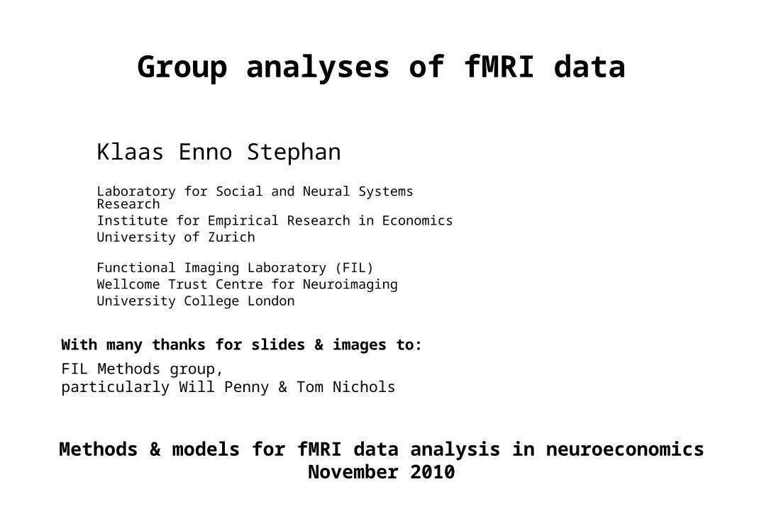
Time
BOLD signalTim
esingle voxel
time series
single voxel
time series
Reminder: voxel-wise time series analysis!
modelspecificati
on
modelspecificati
onparameterestimationparameterestimation
hypothesishypothesis
statisticstatistic
SPMSPM
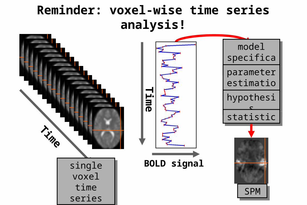
The model: voxel-wise GLM
=
e+yy XX
N
1
N N
1 1p
p
Model is specified by1. Design matrix X2. Assumptions about
e
Model is specified by1. Design matrix X2. Assumptions about
e
N: number of scansp: number of regressors
N: number of scansp: number of regressors
eXy
The design matrix embodies all available knowledge about experimentally controlled factors and potential confounds.
),0(~ 2INe

GLM assumes Gaussian “spherical” (i.i.d.) errors
sphericity = iid:error covariance is scalar multiple of identity matrix:
Cov(e) = 2I
sphericity = iid:error covariance is scalar multiple of identity matrix:
Cov(e) = 2I
10
01)(eCov
10
04)(eCov
21
12)(eCov
Examples for non-sphericity:
non-identity
non-independence

Multiple covariance components at 1st level
),0(~ 2VNe
iiQV
eCovV
)(
= 1 + 2
Q1 Q2
Estimation of hyperparameters with ReML (restricted maximum likelihood).
V
enhanced noise model error covariance components Qand hyperparameters
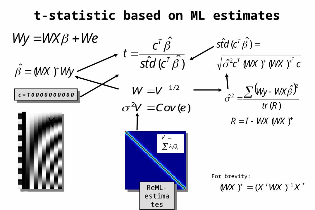
WeWXWy
c = 1 0 0 0 0 0 0 0 0 0 0c = 1 0 0 0 0 0 0 0 0 0 0
)ˆ(ˆ
ˆ
T
T
cdts
ct
cWXWXc
cdtsTT
T
)()(ˆ
)ˆ(ˆ
2
)(
ˆˆ
2
2
Rtr
WXWy
ReML-estimates
ReML-estimates
WyWX )(̂
)(2
2/1
eCovV
VW
)(WXWXIRX
t-statistic based on ML estimates
iiQ
V
TT XWXXWX 1)()( For brevity:
Distribution of population effect
8
Subj. 1
Subj. 2
Subj. 3
Subj. 4
Subj. 5
Subj. 6
0
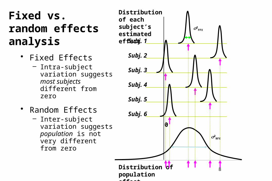
Fixed vs.random effectsanalysis
• Fixed Effects– Intra-subject variation
suggests most subjects different from zero
• Random Effects– Inter-subject variation
suggests population is not very different from zero
Distribution of each subject’s estimated effect 2
FFX
2RFX

Fixed Effects
• Assumption: variation (over subjects) is only due to measurement error
• parameters are fixed properties of the population (i.e., they are the same in each subject)
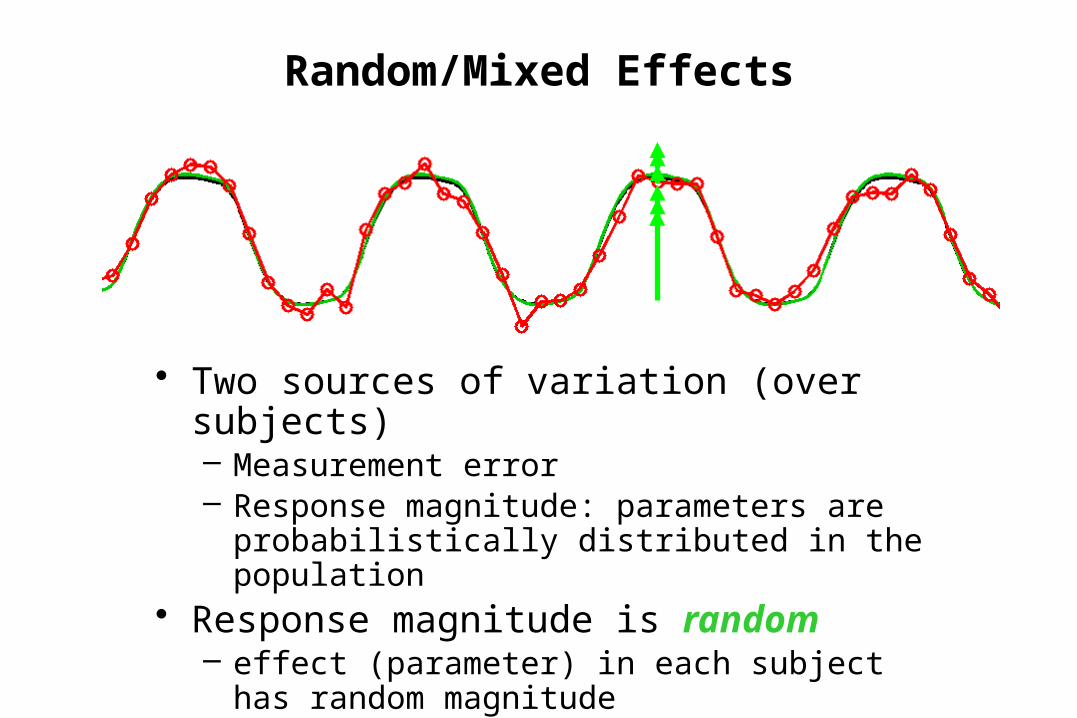
Random/Mixed Effects
• Two sources of variation (over subjects)– Measurement error– Response magnitude: parameters are
probabilistically distributed in the population• Response magnitude is random
– effect (parameter) in each subject has random magnitude

• Two sources of variation– Measurement error– Response magnitude: parameters are
probabilistically distributed in the population• Response magnitude is random
– effect (parameter) in each subject has random magnitude
– variation around population mean
Random/Mixed Effects

Group level inference: fixed effects (FFX)
• assumes that parameters are “fixed properties of the population”
• all variability is only intra-subject variability, e.g. due to measurement errors
• Laird & Ware (1982): the probability distribution of the data has the same form for each individual and the same parameters
• In SPM: simply concatenate the data and the design matrices lots of power (proportional to number of scans),
but results are only valid for the group studied and cannot be generalized to the population

Group level inference: random effects (RFX)
• assumes that model parameters are probabilistically distributed in the population
• variance is due to inter-subject variability
• Laird & Ware (1982): the probability distribution of the data has the same form for each individual, but the parameters vary across individuals
• hierarchical model much less power (proportional to number of subjects), but results can be generalized to the population

Hierachical models
fMRI, single subjectfMRI, single subject
fMRI, multi-subjectfMRI, multi-subject ERP/ERF, multi-subjectERP/ERF, multi-subject
EEG/MEG, single subjectEEG/MEG, single subject
Hierarchical models for all imaging data!
Hierarchical models for all imaging data!
time
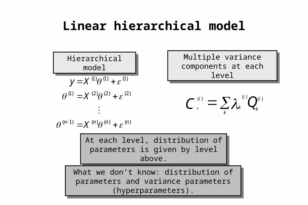
Linear hierarchical model
)()()()1(
)2()2()2()1(
)1()1()1(
nnnn X
X
Xy
)()()( i
k
i
kk
i QC
Hierarchical modelHierarchical model Multiple variance components at each level
Multiple variance components at each level
At each level, distribution of parameters is given by level above.
At each level, distribution of parameters is given by level above.
What we don’t know: distribution of parameters and variance parameters (hyperparameters).
What we don’t know: distribution of parameters and variance parameters (hyperparameters).

Example: Two-level model
=
2221
111
X
Xy
1
1+ 1 = 2X
2
+ 2y
)1(1X
)1(2X
)1(3X
Second levelSecond level
First levelFirst level
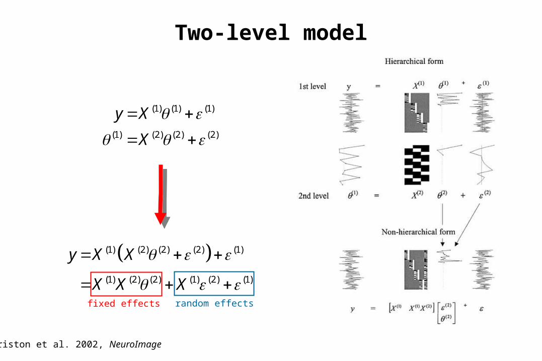
Two-level model
(1) (1) (1)
(1) (2) (2) (2)
y X
X
(1) (2) (2) (2) (1)
(1) (2) (2) (1) (2) (1)
y X X
X X X
Friston et al. 2002, NeuroImage
fixed effects random effects
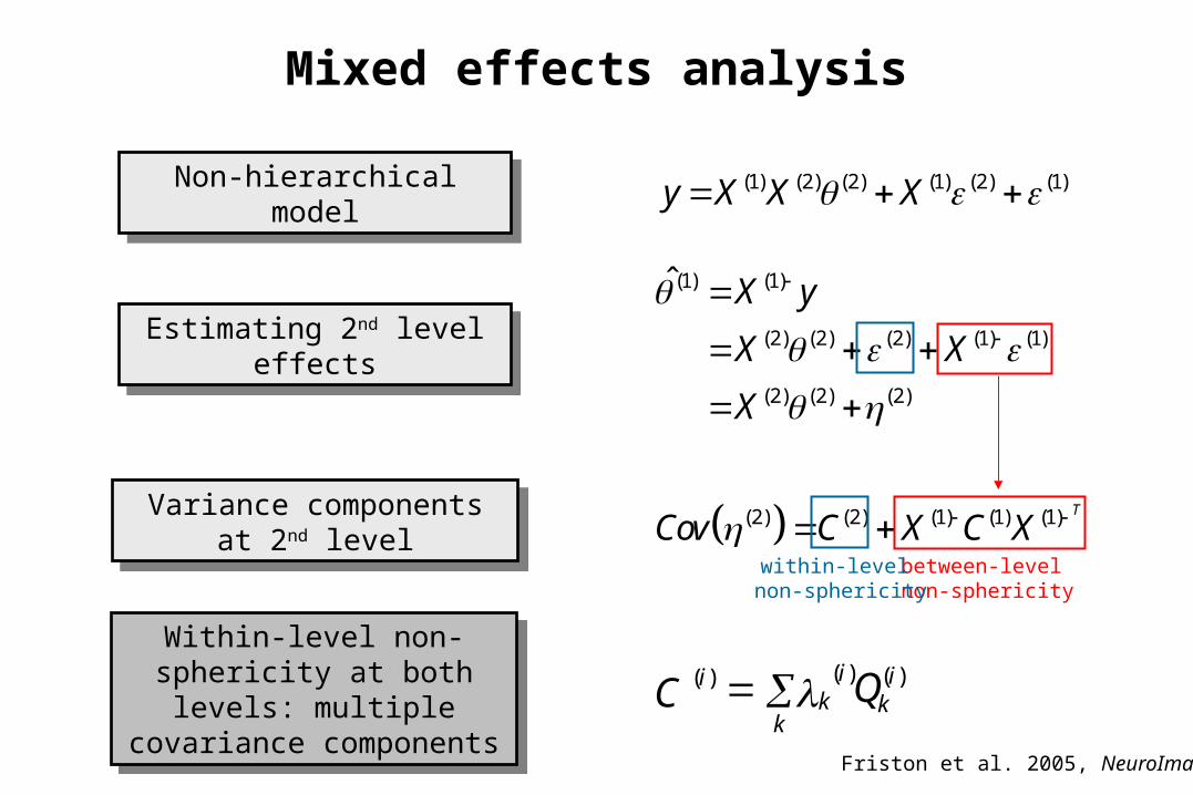
Mixed effects analysis
(1) (2) (2) (1) (2) (1)y X X X
(1) (1)
(2) (2) (2) (1) (1)
(2) (2) (2)
ˆ X y
X X
X
(2) (2) (1) (1) (1) T
Cov C X C X
Non-hierarchical modelNon-hierarchical model
Variance components at 2nd level
Variance components at 2nd level
Estimating 2nd level effectsEstimating 2nd level effects
between-level non-sphericity
( ) ( )( ) i iik k
kQC
Within-level non-sphericity at both levels: multiple
covariance components
Within-level non-sphericity at both levels: multiple
covariance componentsFriston et al. 2005, NeuroImage
within-level non-sphericity

Estimation
EM-algorithmEM-algorithm
gJ
d
LdJ
d
dLg
1
2
2
E-stepE-step
M-stepM-step
kk
kQC
Assume, at voxel j:
Assume, at voxel j: kjjk
maximise L ln ( )p y | λ
111
NppNN
Xy
yCXC
XCXCT
yy
Ty
1||
11| )(
Friston et al. 2002, NeuroImage
GN gradient ascent

Algorithmic equivalence
)()()()1(
)2()2()2()1(
)1()1()1(
nnnn X
X
Xy
Hierarchicalmodel
Hierarchicalmodel
ParametricEmpirical
Bayes (PEB)
ParametricEmpirical
Bayes (PEB)
EM = PEB = ReMLEM = PEB = ReML
RestrictedMaximumLikelihood
(ReML)
RestrictedMaximumLikelihood
(ReML)
Single-levelmodel
Single-levelmodel
)()()1(
)()1()1(
)2()1()1(
...
nn
nn
XXXX
Xy

Practical problems
Most 2-level models are just too big to compute.
Most 2-level models are just too big to compute.
And even if, it takes a long time! And even if, it takes a long time!
Moreover, sometimes we are only interested in one specific effect and do not want to model all the data.
Moreover, sometimes we are only interested in one specific effect and do not want to model all the data.
Is there a fast approximation?Is there a fast approximation?
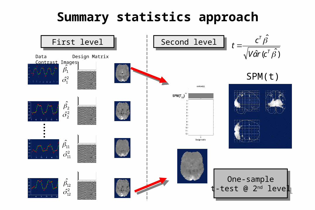
Summary statistics approach
Data Design Matrix Contrast Images )ˆ(ˆ
ˆ
T
T
craV
ct
SPM(t)1̂
2̂
11̂
12̂
21̂
22̂
211̂
212̂
Second levelSecond levelFirst levelFirst level
One-samplet-test @ 2nd level
One-samplet-test @ 2nd level

Validity of the summary statistics approach
The summary stats approach is exact if for each session/subject:
The summary stats approach is exact if for each session/subject:
But: Summary stats approach is fairly robust against violations of these
conditions.
But: Summary stats approach is fairly robust against violations of these
conditions.
Within-session covariance the sameWithin-session covariance the same
First-level design the sameFirst-level design the same
One contrast per sessionOne contrast per session

Mixed effects analysis
Summarystatistics
Summarystatistics
EMapproach
EMapproach
(2)̂
jjj
i
Tii QXQXV
XXY
)2()2()1()1()1()1(
)2(
)1(ˆ
yVXXVX TT 111)2( )(ˆ
yVXXVX TT 111)1( )(ˆ
},,{ QXnyyREML T
Step 1
Step 2
},,,{
][)1()2(
1)1()1(
1
)2()1()0(
TXQXQQ
XXXX
IV
XXX
][ )1()0(
datay
Friston et al. 2005, NeuroImage
non-hierarchical model
1st level non-sphericity
2nd level non-sphericity
pooling over voxels
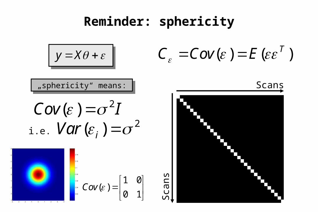
Reminder: sphericity
„sphericity“ means:„sphericity“ means:
ICov 2)(
Xy )()( TECovC
Scans
Sca
ns
i.e.2)( iVar
10
01)(Cov
2nd level: non-sphericity
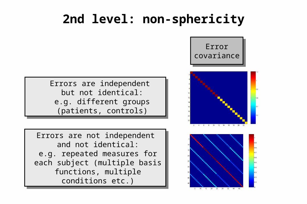
Errors are independent but not identical:
e.g. different groups (patients, controls)
Errors are independent but not identical:
e.g. different groups (patients, controls)
Errors are not independent and not identical:
e.g. repeated measures for each subject (multiple basis functions,
multiple conditions etc.)
Errors are not independent and not identical:
e.g. repeated measures for each subject (multiple basis functions,
multiple conditions etc.)
Errorcovariance
Errorcovariance
2nd level: non-sphericity
27
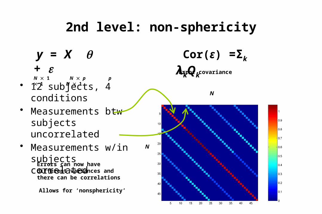
y = X + eN 1 N p p 1 N 1
N
N
Error covariance
Errors can now have different variances and there can be correlations
Allows for ‘nonsphericity’
• 12 subjects, 4 conditions
• Measurements btw subjects uncorrelated
• Measurements w/in subjects correlated
Cor(ε) =Σk λkQk

Example 1: non-identical & independent errors
Stimuli:Stimuli: Auditory Presentation (SOA = 4 secs) of(i) words and (ii) words spoken backwards
Auditory Presentation (SOA = 4 secs) of(i) words and (ii) words spoken backwards
Subjects:Subjects:
e.g. “Book”
and “Koob”
e.g. “Book”
and “Koob”
fMRI, 250 scans per subject, block design
fMRI, 250 scans per subject, block design
Scanning:Scanning:
(i) 12 control subjects(ii) 11 blind subjects
(i) 12 control subjects(ii) 11 blind subjects
Noppeney et al.

1st level:1st level:
2nd level:2nd level:
ControlsControls BlindsBlinds
X
]11[ TcV

Stimuli:Stimuli: Auditory Presentation (SOA = 4 secs) of words Auditory Presentation (SOA = 4 secs) of words
Subjects:Subjects:
fMRI, 250 scans persubject, block design
fMRI, 250 scans persubject, block designScanning:Scanning:
(i) 12 control subjects(i) 12 control subjects
1. Motion 2. Sound 3. Visual 4. Action
“jump” “click” “pink” “turn”
Question:Question:
What regions are generally affected by the semantic content of the words?Contrast: semantic decisions > auditory decisions on reversed words (gender identification task)
What regions are generally affected by the semantic content of the words?Contrast: semantic decisions > auditory decisions on reversed words (gender identification task)
Example 2: non-identical & non-independent errors
Noppeney et al. 2003, Brain
1. Words referred to body motion. Subjects decided if the body movement was slow.
2. Words referred to auditory features. Subjects decided if the sound was usually loud
3. Words referred to visual features. Subjects decided if the visual form was curved.
4. Words referred to hand actions. Subjects decided if the hand action involved a tool.

Repeated measures ANOVA
1st level:1st level:
2nd level:2nd level:
3.Visual3.Visual 4.Action4.Action
X
?=
?=
?=
1.Motion1.Motion 2.Sound2.Sound

Repeated measures ANOVA
1st level:1st level:
2nd level:2nd level:
3.Visual3.Visual 4.Action4.Action
X
?=
?=
?=
1.Motion1.Motion 2.Sound2.Sound
1100
0110
0011Tc
V
X
Practical conclusions
• Linear hierarchical models are used for group analyses of multi-subject imaging data.
• The main challenge is to model non-sphericity (i.e. non-identity and non-independence of errors) within and between levels of the hierarchy.
• This is done by estimating hyperparameters using EM or ReML (which are equivalent for linear models).
• The summary statistics approach is robust approximation to a full mixed-effects analysis.– Use mixed-effects model only, if seriously in doubt about validity of
summary statistics approach.
Recommended reading
Linear hierarchical models
Mixed effect models

Thank you