Group #2 Project Final Report: Information Flows onTwitter

Huang-Wei Chang, Te-Yuan Huang

1 Introduction

Twitter has become a very popular microblog website and had attracted millions of users up to 2009.It is generally considered as a social networking website but gradually also used as a media for peo-ple or companies to spread out news or marketing information. One reason for considering Twitteras a media that broadcasts information instead of a social network is that on Twitter the friendshipbetween two users are asymmetric 1 and according to [1] only 22.1% of the relationships are re-ciprocal. This is very different from the online messenging services such as MSN or Google Chat.However, different from the traditional media like TV or newspapers, a user can easily propagatean information she saw from other users to her followers by retweet, which is an automatic way ofduplicating others’ posts on the reader’s Twitter board. The retweet function is critical for makingthe information available to a large number of users. However, in the online environment, we knowsometimes people see but not really read the content.

Therefore, the topic of our project is to study information flow on Twitter network, especially wewant to understand the role played by the reading rate of a post and retweet rate after the user readsthe message. We construct epidemic models according to the design of Twitter. Our epidemic modelcan better capture the nature of information cascade on the Twitter network. We will further explainour epidemic model in Section 3, here we only briefly describe the model setting.

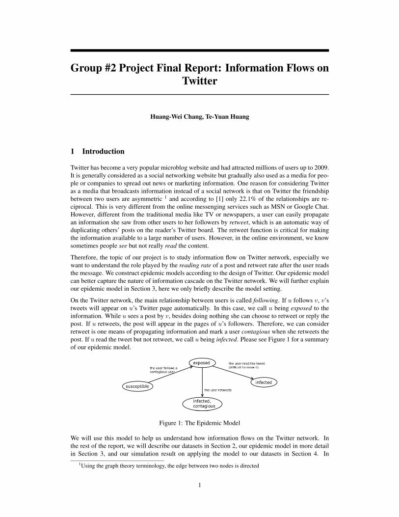
On the Twitter network, the main relationship between users is called following. If u follows v, v’stweets will appear on u’s Twitter page automatically. In this case, we call u being exposed to theinformation. While u sees a post by v, besides doing nothing she can choose to retweet or reply thepost. If u retweets, the post will appear in the pages of u’s followers. Therefore, we can considerretweet is one means of propagating information and mark a user contagious when she retweets thepost. If u read the tweet but not retweet, we call u being infected. Please see Figure 1 for a summaryof our epidemic model.

Figure 1: The Epidemic Model

We will use this model to help us understand how information flows on the Twitter network. Inthe rest of the report, we will describe our datasets in Section 2, our epidemic model in more detailin Section 3, and our simulation result on applying the model to our datasets in Section 4. In

1Using the graph theory terminology, the edge between two nodes is directed

1

Figure 2: Visualization of One Twitter User in Our Log on a Single Day

Section 5, we will further discuss how retweet rate will be impacted by various factors. Then finallyin Section 6, we will summarize our project and describe a few take way ideas.

2 Our Datasets

In this project, we are using two networks: one is collected by ourselves focused on mobile usersin New York City and the other one is build from the dataset released by Kwak et.al [1]. Onefundamental difference between these two networks are the users. For our dataset, we are focusedon general mobile users who use twitter on-the-go; the users involve in the data are common peoplelike you and me. For Kwak’s dataset, they capture the dataset by crawling the twitter networkfrom some popular figures and therefore most of the users in their network has a huge number offollowers. As a result, the network structure of the two networks are very different and it is veryinteresting to see how the network structure impacts on the information diffusion. In this section,we will detail on how we collect the NYC dataset from twitter and how we construct a network fromKwak’s dataset.

2.1 NYC Network: The Retweet Network for Mobile Users in NYC

In order to identify mobile users in New York City, we use Twitter’s APIs to collect all the tweetsgenerated by mobile devices and with GPS location within the NYC. Their geo-location APIs allowsus to collect tweets that are posted within a pre-configured geographical range, and we further usethe name of the twitter client to select the tweets generated by the twitter clients on mobile phones,such as “twitter for iPhone” and “twitter for android”. We collect all these tweets from the 10 mostpopulated cities in the United States, including New York City, Chicago, BayArea, Los Angeles,Houston, Dallas, San Antonio, Phoenix, Philadelphia and San Diego. However, among all the citieswe collect data from, New Yorkers seems to use twitter the most and the most frequent. We cancollect around 40-50MB of tweet from NYC each day. For the rest of the cities, it’s around 10-20MB of tweet per day. Therefore, in the rest of the project, we will use the data from NYC toanalyze how information flows on twitter’s network. Figure 2 is a visualization on one of our users’tweets in one particular day; we plot each tweet according to the geo-location attached to it.

Since we are interested in knowing how the messages are propagated between people, we are alsocollecting the followee/follower relationship of the users in our trace. For each retweet, we wouldlike to know how the tweet is propagated to the user. First of all, we collect whom the user’sfollowing, i.e., the user’s friends in Twitter’s terminology. Secondly, since retweets follows theformat: ”RT @Source: content”, we parse the content of the retweet to retrieve the source of thetweet. After we learn the sources, we collect the sources’ follower. In Figure 3, we plot out the datawe collected and their relationship between each other. In our dataset, there are 440,135 tweets and

2

Figure 3: Data Collection for Building NYC Network

Figure 4: Network built from Kwak’s Dataset

15,919 of them are retweets. The retweets are generated by 1407 unique users, whom we calledseeds; while the sources of the retweets are 8517 unique users, whom we called sources. Amongthe 1407 seeds, 1244 of them allowing us to collect their friend list, and among the 8517 sources,6167 of them allowing us to collect their follower list. After collecting the friends of the seeds andthe followers of the sources, we have roughly 250,000 users (or nodes) and 4,000,000 edges in ournetwork. In other words, this network is very well connected and most of the retweets can travelfrom the sources to the seeds within two steps.

2.2 Kwak Network: The Retweet Network for Users in Kwak’s Dataset

Kwak’s dataset provided the follower/followee relationship between followers and followees for 20million users. However, in order to make a network comparable with the NYC network, we try toselect a subset of Kwak’s network and make the number of edges is at the same scale as the NYCNetwork.

Following is how we select the subset and the procedure is also plotted in Figure 4. First, werandomly pick 50 users. Secondly, we include in their followers and finally the followers of thesefollowers. In the end, we have roughly 2,000,000 users and 8,000,000 of edges (i.e., the followingrelationships). To compare with the NYC network, which has 250,000 nodes and 4,000,000 edges,Kwak Network is more flat (i.e., each users have lots more followers), and less inter-connected.

3

Figure 5: Diffusion Model Mode 0

Figure 6: Diffusion Model Mode 1

3 Epidemic Models

In this section, we are going to model users’ reaction to tweets. However, since we don’t really knowusers’ behavior, we come up with three different diffusion models based on our own experience. Inour models, we have four states: susceptible, exposed, infected and contagious.

• Susceptible: a user is susceptible to a post when s/he is following a contagious user

• Exposed: a user is exposed to a tweet when the tweet shows up on his/her twitter page.

• Infected: a user is infected by a post when s/he read the tweet

• Contagious: a user is contagious when s/he retweet the tweet, i.e., his/her follower wouldbecome susceptible and exposed to the tweet as well.

3.1 Mode 0

Mode 0 is the simplest model. As soon as a friend of u generates a new tweet, u becomes susceptibleand then automatically exposed to the tweet. Then, with a probability, named infection rate, the userwould read the tweet. That is, the user would become infected with the probability of infection rate.After the user has read the tweet, there is also a probability, named contagious rate or retweet rate,that the user retweets the post, become contagious and makes his/her followers become susceptible.We summarize this mode in Figure 5.

Please note that in this model, the user has only one chance to decide whether it will be infected orcontagious. Even when the tweet reappears on his/her twitter page through another route, the userwon’t change his/her decision.

3.2 Mode 1

Mode 1 is similar to the mode 0; however, if the same tweet appears on the user’s page the secondtime, we assume that the user has another chance to decide whether she will read it or even retweetit. However, if the user has already read the tweet before and has decided not to retweet it. Then, inmode 1, the reappearance of the tweet would not change the user’s decision. Mode 1 is summarizedin Figure 6.

4

Figure 7: Diffusion Model Mode 2

3.3 Mode 2

Mode 2 is developed based on our observation that users’ decision would also be influenced byother users’ decision. Imagine a user originally decided not to retweet a post, which many of hisfriend later decided to retweet it. After seeing most of his friend’s decision, the user might changeits decision from only being infected to contagious. Thus, in mode 2, when a tweet reappear tothe user’s page, we give the infected user also another change to decide whether s/he would like tobecome contagious or not. Mode 2 is summarized in Figure 7.

4 Simulation Result

In order to simulate how the information propagates in the twitter network, we would need to decidethe infection rate and contagious rate (or retweet rate). We are able to calculate retweet rate fromour NYC dataset, which is around 0.03. However, it is very hard to determine the infection rate fromthe empirical data. In the following simulation, we fix infection rate at 0.3 and will briefly discussthe impact of different infection rates.

4.1 For NYC Network

We run the simulation by inject a message at a number of sources in the network, and calculatethe number of seeds (out of the 1244 seeds) will become exposed/infected/contagious at the end ofsimulation. The simulation results for NYC Network is shown in Figure 8. The x-axis is the numberof sources that we inject the information initially, and the y-axis is the number of seeds. The red linepresents the number of exposed nodes, the blue line presents the number of infected nodes, and theblack line presents the number of contagious nodes. If we compare mode 0 to the other two modes,we can see that the number of infected and contagious nodes are much less than mode 1 and mode2. This is because, in mode 0, the user only has one chance to decide whether s/he would like toread/retweet the post, even when the tweet showed up several times in the page. Also, since ourNYC Network is very well connected, we find that the difference between the number of exposednodes and infected nodes is very small. This is because most of the nodes would receive the tweetmore than once and therefore have greater chance to become infected/contagious.

We further investigate how different infection rates would impact on the number of infected nodes.We apply different infection rates on the NYC Network and the results are shown in Figure 9. Fromthe result, we can see that infection rates indeed has huge impact on the number of infected node.

4.2 For Kwak’s Network

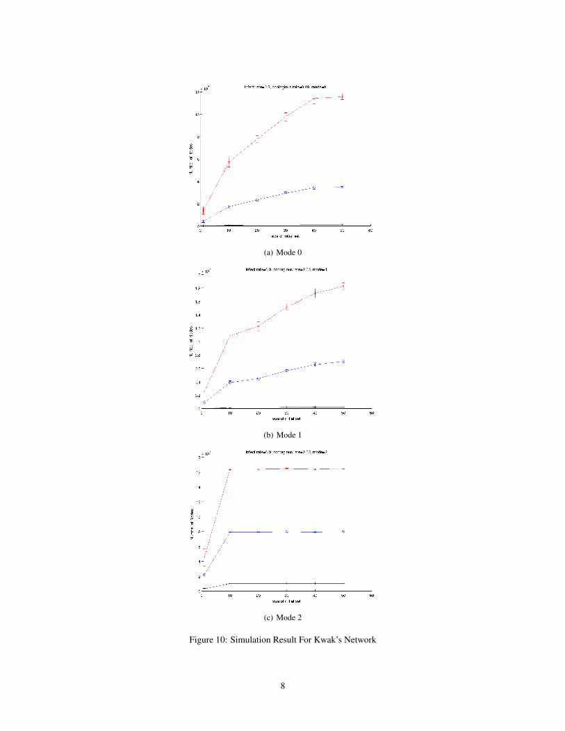
We run the similar simulation on Kwak’s Network, and present the result in Figure 10. Similar to theresult in the NYC Network, mode 0 has the least number of nodes to be exposed/infected/contagious.However, different from the result in the NYC Network, even in mode 2, the difference between the

5

(a) Mode 0

(b) Mode 1

(c) Mode 2

Figure 8: Simulation Result For NYC Network

6

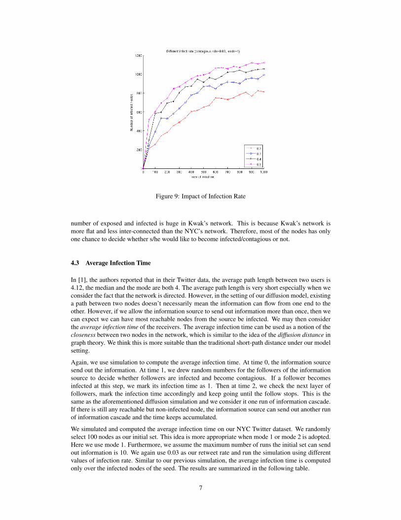
Figure 9: Impact of Infection Rate

number of exposed and infected is huge in Kwak’s network. This is because Kwak’s network ismore flat and less inter-connected than the NYC’s network. Therefore, most of the nodes has onlyone chance to decide whether s/he would like to become infected/contagious or not.

4.3 Average Infection Time

In [1], the authors reported that in their Twitter data, the average path length between two users is4.12, the median and the mode are both 4. The average path length is very short especially when weconsider the fact that the network is directed. However, in the setting of our diffusion model, existinga path between two nodes doesn’t necessarily mean the information can flow from one end to theother. However, if we allow the information source to send out information more than once, then wecan expect we can have most reachable nodes from the source be infected. We may then considerthe average infection time of the receivers. The average infection time can be used as a notion of thecloseness between two nodes in the network, which is similar to the idea of the diffusion distance ingraph theory. We think this is more suitable than the traditional short-path distance under our modelsetting.

Again, we use simulation to compute the average infection time. At time 0, the information sourcesend out the information. At time 1, we drew random numbers for the followers of the informationsource to decide whether followers are infected and become contagious. If a follower becomesinfected at this step, we mark its infection time as 1. Then at time 2, we check the next layer offollowers, mark the infection time accordingly and keep going until the follow stops. This is thesame as the aforementioned diffusion simulation and we consider it one run of information cascade.If there is still any reachable but non-infected node, the information source can send out another runof information cascade and the time keeps accumulated.

We simulated and computed the average infection time on our NYC Twitter dataset. We randomlyselect 100 nodes as our initial set. This idea is more appropriate when mode 1 or mode 2 is adopted.Here we use mode 1. Furthermore, we assume the maximum number of runs the initial set can sendout information is 10. We again use 0.03 as our retweet rate and run the simulation using differentvalues of infection rate. Similar to our previous simulation, the average infection time is computedonly over the infected nodes of the seed. The results are summarized in the following table.

7

(a) Mode 0

(b) Mode 1

(c) Mode 2

Figure 10: Simulation Result For Kwak’s Network

8

Infection Rate Infected nodes Avg Infection time0.1 516 16.560.2 642 8.350.3 774 5.70.4 821 4.030.5 909 2.88

Table 1: The Impact of Infection Rates

5 Learning The Retweet Rate Prediction Function

There are two main parameters in our epidemic model: the infection rate, which is the probabilityfor the user to read a post from whom the user follows, and the contagion rate (or retweet rate),which is the probability for the user to retweet a post after reading it. As we have shown in previoussections, the information cascade on the Twitter network is decided by the two parameters.

In stead of fitting the parameters of the network for each edge in the Twitter network, we wantto learn functions to predict the rates for a given pair of Twitter following information. Using theTwitter API, we can obtain the posts by a given user. Furthermore, if a post is a retweet instead ofan original post by this user, there will be a mark ”RT“ before it. Therefore, we can estimate theoverall retweet rate. Even more, the retweet posts also record who is the source. Therefore, fix apair of users (u, v), in which u follows v, we can compute the retweet rate between them.

On the other hand, it is difficult to know whether a user read a post from whom she follows, becausethe user can take no action on Twitter even she indeed read the post. Therefore, estimating theinfection rate is not an easy task. As a result, here we focus on learning the retweet rate from thedata and assume the infection rate is 1.

5.1 The Prediction Function and Cost Functions in The Learning Algorithm

To be specific, we select a set of (directed) edges E′ in the NYC network, in which for each edge(u, v) in E′ there exists at least one retweet 2. We use the profile of u and v as the input (features)and compute the retweet rate of (u, v) as the output of a linear function f . Denote the features of thei-th edge in our dataset as x(i) and the retweet rate to be r(i). The features we used in the predictionfunction includes the following information of both u and v:

status count The number of tweets the user has.

followers count How many people follow this user.

friend count How many people the user follows.

retweet count How many retweets the use made before.

time zone The time zone of the user.

We want to learn the coefficients α of f(x) = αTx so that f(x(i)) is close to r(i). For the close-ness we can use the least square distance. Besides, since the rate is the parameter of a Bernulidistribution, we can compute the KullbackLeibler divergence (KL-divergense) or the Bhattacharyyadistance between the distributions as the distance. To sum up, we use the following three differentcost functions for f(x(i)) and r(i):

Least square distance :‖f(x)− r‖2

2Therefore, what the model really learned is the retweet rate given that the follower ever retweeted.

9

KullbackLeibler divergence :

DKL = f(x) logf(x)

r+ (1− f(x)) log (1− f(x))

1− r

Bhattacharyya distance : √f(x)r +

√(1− f(x))(1− r)

For the case of using least-square distance, we solved it as a linear regression problem using thepackage in Matlab. For the other two cost functions, we do the optimization using gradient descent.

5.2 Evaluation

To evaluate the learned prediction function, we compute the log-likelihood of our data; that is,

|E′|∑i=1

[#reweet(u(i), v(i))× log f(x(i)) + (#post(v(i))−#reweet(u(i), v(i)))× log(1− f(x(i)))

].

Besides the aforementioned three models using different cost functions, we also compute the log-likelihood using the total average retweet rate for comparison. The table below is the result:

Least sequare KL-divergence Bhattacharyya AvgNYC -68.7986 -70.2389 -70.0540 -93.2763

Besides the log-likelihood values, we also discovered an interesting fact in our dataset. In our learnedmodel learned from the NYC dataset, we found the the number of posts of the information sourcehas negative relationship with the infection rate. We guess this might be because that the users witha huge number of posts are some news media which post very often but not all tweet were read(infection rate is less than 1).

6 Summary

To sum up, during the past several weeks we did the data preparation and preprocessing. Besides,we also investigated the data to figure out what kind of learning model and features we can use topredict the model parameters. The model parameters and the coefficients of the prediction functionsshould be able to reflect some interesting properties of information cascade on Twitter network.

Remark

In our original proposal, we assume the infection rate to be the sum of retweet rate 3 and replyrate. However, after investigating our dataset, we found the obtained infection rate is too low to berealistic. Therefore, we decided to use the model mentioned in this report.

References

[1] Kwak H., Lee C., Park H., Moon S. (2010), Proceedings of the 19th International World Wide Web (WWW)Conference

3It is defined directly as the ratio of total number of retweet over total number of post as in our learningmodel instead of the definition we used in our final model

10