GROUNDWATER MONITORING, EVALUATION AND GROWER...
95
Transcript of GROUNDWATER MONITORING, EVALUATION AND GROWER...


THE UNIVERSITY OF NEW SOUTH WALES SCHOOL OF CIVIL AND ENVIRONMENTAL ENGINEERING
WATER RESEARCH LABORATORY
IN ASSOCIATION WITH GHD HASSALL
GROUNDWATER MONITORING, EVALUATION AND GROWER SURVEY, NAMOI CATCHMENT
Report No. 2
PART A: RESULTS OF 2009 GROUNDWATER MONITORING AND RECOMMENDATIONS FOR FUTURE BEST PRACTICE
MONITORING FRAMEWORK
PART B: GROUNDWATER USER SURVEY
WRL Technical Report 2009/25 April 2010
by
W A Timms, A M Badenhop, D S Rayner and S M Mehrabi

Water Research Laboratory School of Civil and Environmental Engineering Technical Report No 2009/25 University of New South Wales ABN 57 195 873 179 Report Status Final King Street Date of Issue April 2010 Manly Vale NSW 2093 Australia Telephone: +61 (2) 9949 4488 WRL Project No. 08085 Facsimile: +61 (2) 9949 4188 Project Manager W A Timms
Title Groundwater Monitoring, Evaluation and Grower Survey, Namoi
Catchment, Report No. 2 Part A: Results of 2009 Groundwater Monitoring and Recommendations for Future Best Practice Monitoring Framework Part B: Grower Survey
Author(s) W A Timms, A M Badenhop, D S Rayner and S M Mehrabi Reviewed by B Kelly and B M Miller Client Name Cotton CRC and Namoi Catchment Management Authority Client Address Client Contact Client Reference
The work reported herein was carried out at the Water Research Laboratory, School of Civil and Environmental Engineering, University of New South Wales, acting on behalf of the client. Information published in this report is available for general release only with permission of the Director, Water Research Laboratory, and the client.

WRL TECHNICAL REPORT 2009/25
-i-
GLOSSARY OF TERMS
Baseline Baseline conditions are the range of values that are representative of a
system prior to a certain reference point eg. a new development or
legislative date. By definition, values outside of baseline conditions
can only occur if there has been a change to the system.
Benchmark A standard or point of reference by which progress can be measured.
In this report, the benchmark aims to reflect the baseline conditions of
the catchment.
Beneficial use The purpose for which water may be used as governed by the quality of
the water. Also defined as ‘environmental value’ in the NSW
Groundwater Protection Policy (DLWC,1998); beneficial uses may
include ecosystem protection, recreation and aesthetics, raw water for
drinking water supply, agricultural water, and industrial water.
BMP Best management practice
Catchment Target Catchment Targets are “a statement of future goals about the desired
condition of the resource” providing a “broad indicator of catchment
health” (Namoi CMA, 2007).
CMA Catchment Management Authority
CWI Connected Waters Initiative http://www.connectedwaters.unsw.edu.au/
DECCW Department of Environment, Climate Change and Water (formerly
Department of Water and Energy, DWE)
DO Dissolved oxygen
EC Electrical Conductivity
GDE Groundwater dependant ecosystem
GWMA Groundwater Management Area, also referred to as Groundwater
Management Unit, GMU
SAR Sodium Adsorption Ratio
SWL Standing water level
TDS Total dissolved solids
Trigger A trigger is a means of defining whether change has occurred within a
system, such that a management action is required or ‘triggered’. By
this definition, a trigger is a methodology for determining significant
change within a system. This methodology may include, but is
certainly not limited to, setting a specific hard ‘trigger value’ that
cannot be exceeded.
UCL Upper Cutoff Limit – a type of trigger that can be used as hard limit;
above this value a management action may be triggered.

WRL TECHNICAL REPORT 2009/25
-i-
CONTENTS
EXECUTIVE SUMMARY
1. INTRODUCTION 1 1.1 Scope of Work 2 1.2 Report Structure 2
2. REVIEW OF GROUNDWATER INDICATORS AND TARGETS 4 2.1 Catchment Management Targets in the Namoi 5 2.2 Beneficial Uses for Groundwater 6 2.3 Monitoring Groundwater to Manage Catchment Management Targets 8
2.3.1 Appropriate Triggers to Identify Significant Changes 9 2.3.2 Statistically Valid Techniques for Analysing Limited Amounts of Data 11
3. CONNECTIVITY INDEX TO DEFINE MONITORING UNITS 13
4. GROUNDWATER MONITORING 2009 16 4.1 Groundwater Sampling by Growers 16
4.1.1 Sampling Method 17 4.1.2 Results 17
4.2 Groundwater Sampling of Monitoring Bores 21 4.2.1 Sampling Method 23 4.2.2 Results 24
4.3 Comparison of Groundwater Quality from Growers and Monitoring Bores 34
5. RISKS TO GROUNDWATER IN THE NAMOI CATCHMENT 36 5.1 Beneficial Uses 36 5.2 Risk Factors 37 5.3 Risks Areas in the Namoi Catchment 39
5.3.1 Water Quality 39 5.3.2 Water Levels 40 5.3.3 Combined Risks 48
5.4 Recommendations for Future Surveys 49
6. STRATEGIES FOR BEST PRACTICE GROUNDWATER MONITORING 50 6.1 Groundwater Monitoring Strategy Concepts 50
6.1.1 Levels of Best Management Practice 50 6.1.2 Purpose of Groundwater Monitoring 51 6.1.3 Frequency and Duration of Monitoring for Various Purposes 51 6.1.4 Sampling 51 6.1.5 Data Analysis 52
6.2 Catchment Scale Groundwater Monitoring 52 6.2.1 Purpose of Monitoring 52 6.2.2 Data Report Card Across the Catchment 53 6.2.3 Site Selection 55 6.2.4 Parameters 57 6.2.5 Frequency of Monitoring 57 6.2.6 Sampling 58 6.2.7 Data Analysis 58 6.2.8 Database Development and Accessibility 59
6.3 Grower Groundwater Monitoring 59

WRL TECHNICAL REPORT 2009/25
-ii-
6.4 Identifying Risk and Resource Degradation 62 6.4.1 Risk Triggers 62 6.4.2 Data Evaluation 65
6.5 Monitoring Program Review 65
7. SUMMARY AND RECOMMENDATIONS 66 7.1 Summary - Groundwater Monitoring and Evaluation 66 7.2 Summary - Grower Survey 70 7.3 Estimated Costs of Strategic Groundwater Quality Monitoring 72 7.4 Community Groundwater Monitoring 74 7.5 Technical Recommendations 75
8. REFERENCES 77 APPENDIX A1 Statistical Techniques for Data Analysis
APPENDIX A2 Connectivity Method of Defining Monitoring Units
APPENDIX A3 Groundwater Sampling in July Information Pack
APPENDIX A4 Groundwater Sampling in July Example Results Report
APPENDIX A5 WRL Target Monitoring Bores
APPENDIX A6 Monitoring Bore Sampling Procedures
APPENDIX A7 WRL Monitoring Results – Tables and Maps
APPENDIX A8 Water Quality Laboratory Results (ALS)
APPENDIX A9 Fact Sheet - DIY Groundwater Monitoring
APPENDIX A10 Database Standards and Information
APPENDIX A11 Presentation Slides from Grower Workshop

WRL TECHNICAL REPORT 2009/25
-iii-
LIST OF TABLES
1. Salinity Guidelines for Key Beneficial Uses in the Namoi Catchment
2. Distribution of Monitored Bores in Upper and Lower Monitoring Units
3. Growers Samples - Accuracy of Bore Locations
4. Growers Samples - EC Results
5. Statistical Summary of Grower Samples Analysis
6. Correlation Analysis (r2 value) for EC, TDS, Na+, Cl-, SAR, and Hardness as
CaCO3 for Growers Samples
7. Summary of Monitoring Bore Sampling by WRL
8. WRL Monitoring EC Results Summary
9. Statistical Summary of WRL Samples Analysis
10. Correlation Analysis for EC, TDS, Na+, Cl-, SAR, and Hardness as CaCO3 for
WRL Samples
11. Summary of Groundwater EC Changes in Monitoring Bores
12. Groundwater Monitoring Bores with Significant EC Variation
13. EC Comparison Between Adjacent Grower and Monitoring Samples
14. Groundwater Salinity at Monitoring Bores in Zone 3
15. Beneficial Use Range
16. Change of Beneficial Use in the Namoi Catchment
17. Summary of Hydrograph Analysis for the Upper and Lower Namoi Alluvium
18. Bores with Recovery Decline Indicating Possible Risk of Consolidation
19. Water Quality Data Availability from Monitoring Bores across the Namoi
Catchment
20. What Sites Should be Monitored in the Namoi Catchment for BMP Groundwater
Monitoring?
21. What Parameters Should be Monitored in the Namoi Catchment for BMP
Groundwater Monitoring?
22. How Frequently Should Water Level be Monitored in the Namoi Catchment for
BMP Groundwater Monitoring?
23. How Frequently Should Water Quality Parameters be Monitored in the Namoi
Catchment for BMP Groundwater Monitoring?
24. Practical vs Statistical Significance of EC Change – An Examination of Suggested
Triggers
25. Estimated Costs of Strategic Monitoring

WRL TECHNICAL REPORT 2009/25
-iv-
LIST OF FIGURES
1. Namoi Catchment
2. Grower Sample Sites
3. Salinity across Grower Sites
4. SAR-EC Growers Samples
5. Target Groundwater Monitoring Bores
6. SWL (mbg) - WRL Monitoring Round 1 - Upper Monitoring Unit
7. SWL (mbg) - WRL Monitoring Round 2 - Upper Monitoring Unit
8. SWL (mbg) - WRL Monitoring Round 3 – Upper Monitoring Unit
9. SWL (mbg) - WRL Monitoring Round 1 - Lower Monitoring Unit
10. SWL (mbg) - WRL Monitoring Round 2 - Lower Monitoring Unit
11. SWL (mbg) - WRL Monitoring Round 3 - Lower Monitoring Unit
12. Groundwater Levels (mAHD)- WRL Monitoring Round 1 - Upper Monitoring Unit
13. Groundwater Levels (mAHD)- WRL Monitoring Round 1 - Lower Monitoring Unit
14. Salinity - WRL Monitoring Round 1 – Upper Monitoring Unit
15. Salinity - WRL Monitoring Round 2 - Upper Monitoring Unit
16. Salinity - WRL Monitoring Round 3 - Upper Monitoring Unit
17. Salinity - WRL Monitoring Round 1 - Lower Monitoring Unit
18. Salinity - WRL Monitoring Round 2 - Lower Monitoring Unit
19. Salinity - WRL Monitoring Round 3- Lower Monitoring Unit
20. Salinity Comparison Between Surface Water Sites and Neighbouring Monitoring Bores
21. SAR-EC WRL Monitoring 2009
22. SWL & EC, WRL Monitoring 2009 – Lower Namoi Alluvium
23. SWL & EC, WRL Monitoring 2009 – Upper Namoi Alluvium, Zone 2
24. SWL & EC, WRL Monitoring 2009 – Upper Namoi Alluvium, Zone 3 & Zone 4
25. SWL & EC, WRL Monitoring 2009 – Upper Namoi Alluvium, Zone 5 & Zone 8
26. SWL & EC, WRL Monitoring 2009 – Peel Valley Alluvium, Upper Monitoring Unit
27. Beneficial Use Based on Salinity – Upper Monitoring Unit
28. Beneficial Use Based on Salinity – Lower Monitoring Unit
29. Beneficial Use Based on Salinity – Deeper Monitoring Unit
30. Average Groundwater Usage 2002-2007 in the Lower Namoi
31. Namoi Soil Salinity
32. Variation in Groundwater Salinity (TDS) from 1970’s to 1990’s in Zone 3
33. Salinity Change Upper Monitoring Unit - Averages of 1980-1999 Compared with 2000-2009
34. Salinity Change Upper Monitoring Unit (Upper Namoi)- Averages of 1980-1999 Compared with 2000-2009
35. Salinity Change Upper Monitoring Unit (Lower Namoi) - Averages of 1980-1999 Compared with 2000-2009

WRL TECHNICAL REPORT 2009/25
-v-
36. Salinity Change Lower Monitoring Unit - Averages of 1980-1999 Compared with 2000-2009
37. Representative bores in the Namoi Catchment for Hydrograph Analysis
38. Hydrographs 1970’s to Mid 2008, Upper Namoi – Zone 1
39. Hydrographs 1970’s to Mid 2008, Upper Namoi – Zone 2
40. Hydrographs 1970’s to Mid 2008, Upper Namoi – Zone 3
41. Hydrographs 1970’s to Mid 2008, Upper Namoi – Zone 4
42. Hydrographs 1970’s to Mid 2008, Upper Namoi – Zone 5 & 11
43. Hydrographs 1970’s to Mid 2008, Upper Namoi – Zone 5 & 11 (Continued)
44. Hydrographs 1970’s to Mid 2008, Upper Namoi – Zone 6 & 10
45. Hydrographs 1970’s to Mid 2008, Upper Namoi – Zone 7
46. Hydrographs 1970’s to Mid 2008, Upper Namoi – Zone 8
47. Hydrographs 1970’s to Mid 2008, Upper Namoi – Zone 9
48. Hydrographs 1970’s to Mid 2008, Upper Namoi – Zone 12
49. Hydrographs 1970’s to Mid 2008, Lower Namoi
50. Hydrographs 1970’s to Mid 2008, Lower Namoi (Continued)
51. Groundwater Level Change 1978 – 2006 (Recovered), Upper Monitoring Unit, Upper Namoi
52. Groundwater Level Change 1978 – 2006 (Recovered), Upper Monitoring Unit, Upper Namoi – Zone 3
53. Groundwater Level Change 1978 – 2006 (Recovered), Upper Monitoring Unit, Lower Namoi
54. Groundwater Level Change 1988 – 2006 (Recovered), Upper Monitoring Unit, Upper Namoi
55. Groundwater Level Change 1978 – 2006 (Recovered), Lower Monitoring Unit, Upper Namoi
56. Groundwater Level Change 1978 – 2006 (Recovered), Lower Monitoring Unit, Upper Namoi – Zone 3
57. Groundwater Level Change 1978 – 2006 (Recovered) Lower Monitoring Unit, Lower Namoi
58. Groundwater Level Change 1988 – 2006 (Recovered). Lower Monitoring Unit, Upper Namoi
59. Groundwater Level Change 2006 – 2008 (Recovered), Upper Monitoring Unit, Upper Namoi
60. Groundwater Level Change 2006 – 2008 (Recovered), Upper Monitoring Unit, Upper Namoi – Zone 3
61. Groundwater Level Change 2006 – 2008 (Recovered), Upper Monitoring Unit, Lower Namoi
62. Groundwater Level Change 2006 – 2008 (Recovered), Lower Monitoring Unit, Upper Namoi
63. Groundwater Level Change 2006 – 2008 (Recovered), Lower Monitoring Unit, Upper Namoi – Zone 3

WRL TECHNICAL REPORT 2009/25
-vi-
64. Groundwater Level Change 2006 – 2008 (Recovered), Lower Monitoring Unit, Lower Namoi
65. Historical Water Level and Salinity Data – GW036213 & GW036151
66. Historical Water Level and Salinity Data – GW036166 & GW036190
67. Historical Water Level and Salinity Data – GW036200
68. Design of Monitoring Bores and Irrigation Bores
69. Historical EC of Example Bores Showing Mann Kendall Trends

WRL TECHNICAL REPORT 2009/25
-i-
EXECUTIVE SUMMARY
Monitoring of groundwater levels and groundwater quality is essential to ensure that this
resource continues to be the life blood of the Namoi catchment and communities. Low
salinity groundwater must be maintained at levels that are accessible for the environment,
drinking water supplies, stock water and for irrigation, supporting an industry worth at least
$380 million each year. This project has helped define how groundwater levels and salinity
vary both spatially and temporally within the catchment. Data sets used for the analyses
were both historical and newly collected from production bores and key state government
groundwater monitoring bores.
The project was completed by the Water Research Laboratory (WRL) projects team of the
University of New South Wales, in association with GHD Hassall, on behalf of the Cotton
Catchment Communities CRC and the Namoi Catchment Management Authority.
Groundwater samples were collected by 79 growers from their production bores and WRL
staff sampled priority state government groundwater monitoring bores in January, March
and July 2009. Standard protocols were used to test ~60 samples at 45 bores on each
occasion with a total of 189 field parameter records and 121 major ion analyses.
It was found that groundwater recovery levels each season remain relatively low compared
to pre-extraction levels in many areas, although there are signs that drawdown levels have
stabilised in other areas since 2006. Groundwater level drawdown appears to have
stabilised in Zone 3 of the Upper Namoi and the unconfined aquifer of Cox’s Creek.
Groundwater salinity was relatively stable at most sites where sufficient historic data was
available (105 monitoring pipes), however, significant groundwater salinity increases have
occurred over the past two decades at about 20% of sites. Freshening had occurred at about
25% of sites that had sufficient data over the same period. However, it is of concern that
some sites in Zone 3 of the Upper Namoi have become significantly more saline, some of
which exceeded guideline values. The worst case was a 123% EC increase up to 2009 with
groundwater at 80 m depth that had become too saline for irrigation of cotton. Yet
groundwater in grower bores several kilometres away was found to be fresh, so further
investigation of this finding is required.
A risk assessment of groundwater resources in the Namoi identified four areas where
changes in salinity might occur in the future that require strategic monitoring. Available
information including the distribution of salt stores in shallow sediments, indicates that the
groundwater resource is at risk in areas of high usage in parts of the Upper Namoi alluvium
(Zone 3 and 8) and Lower Namoi alluvium (north of Wee Waa and near Wee Waa). There

WRL TECHNICAL REPORT 2009/25
-ii-
is currently insufficient baseline groundwater quality data to establish robust trigger values,
although in the interim a >10% EC increase in a bore would provide an early warning
indicator of changes.
Interviews and workshops were used to survey grower attitudes, identifying a priority need
to improve communication of groundwater information, particularly at the start of each
irrigation season. The survey also found a widespread interest in developing and promoting
protocols for groundwater users to gather and track their own groundwater data. Another
priority recommendation was to supplement NSW Office of Water data with additional
independent monitoring of groundwater quality. Most groundwater users had a good to
reasonable understanding of groundwater issues but a limited knowledge of the current
condition of the resource. Some growers expressed a desire for real-time data, such as the
new telemetry program by NSW Office of Water if real time data for local areas can be
accessed through the web. A community program for groundwater monitoring may be
successful in some areas, although there were reservations expressed regarding how data
might be used and the reliability of data. Recommendations of the grower survey and
workshops focused on improving the communication of information about groundwater
conditions and promoting groundwater users to gather and track their own groundwater
quality and levels.
In response to this feedback, the project further developed strategic monitoring guidelines
with a 4 level Best Management Practice (BMP) for irrigation bore monitoring and a 3 level
guideline for subcatchment and regional scale. The BMP for irrigation bores will form part
of the myBMP program for the Cotton Catchment Community CRC. For example, a level
2 BMP is to maximise crop yields by using bore water within appropriate salinity
guidelines. On a regional scale, the current standard at which the monitoring of
groundwater levels is collected and reported is satisfactory for examining long term trends
in water levels. There is a small existing program to upgrade some of the monitoring
network to a telemetry system. This report supports the new telemetry project and suggests
it should be extended. There is also a need for new monitoring of groundwater zones
within the catchment not impacted by irrigation extractions for examining in influence of
climatic variability and change on groundwater recharge. However, regular monitoring of
groundwater quality is currently limited to field parameters and major ion data at a few
locations at an estimated cost of $40,000 to $80,000 per year.
To date the monitoring of water quality has been irregular, making statistical analysis
difficult. It is recommended that the standard of groundwater quality monitoring is
strategically increased to at least a moderate practice at an estimated cost in the order of

WRL TECHNICAL REPORT 2009/25
-iii-
$100,000 to $200,000 per year. A moderate standard of groundwater quality monitoring
would include testing of field parameters (standing water level, electrical conductivity, pH
and temperature) and major ions at approximately 60 key monitoring pipes twice per year,
focused in areas where salinity increases have occurred, or may occur in the future. An
enhanced moderate standard with quarterly testing would improve confidence levels of
statistical baseline parameters, at a cost of approximately $200,000 to $300,000 per year.
These monitoring costs compare with an estimated $480,000 per year of groundwater
access and usage fees for users of the Namoi alluvium sources. A high standard of
groundwater quality (which has not been costed) would include more widespread testing in
areas of the catchment that do not currently have monitoring infrastructure, and could
include other water quality parameters such as nutrients.
Investing in strategic groundwater quality monitoring by individual growers and at a
regional scale is vital to ensuring continued access to fresh groundwater resources by all
users including the environment. Strategic groundwater quality monitoring is a critical
component of the total investment in monitoring, investigating, modelling and managing
groundwater resources across the entire Namoi catchment.

WRL TECHNICAL REPORT 2009/25
-i-
PART A:
RESULTS OF 2009 GROUNDWATER MONITORING AND RECOMMENDATIONS FOR FUTURE BEST PRACTICE MONITORING
FRAMEWORK

WRL TECHNICAL REPORT 2009/25 1.
1. INTRODUCTION
The Namoi region of north-eastern NSW is based around the Namoi, Manilla and Peel
Rivers and contains the major regional centres of Tamworth, Gunnedah, Narrabri, Boggabri
and Wee Waa (Figure 1). Groundwater resources are mostly sourced from deeper alluvial
deposits associated with the main rivers and prior streams; these are often overlain with
relatively saline or brackish waters. Groundwater in the Namoi catchment supports an
irrigation industry worth in excess of $380 million as well as being the water supply for
many towns and intensive industries such as feedlots. Groundwater resources in the region
are the most intensively developed in NSW (CSIRO, 2007) with 2004/2005 groundwater
extraction of 255 GL. Lake Goran is the only wetland of national significance in the area.
Monitoring the status of groundwater levels and groundwater salinity is central to
groundwater management. To better understand this, the Cotton Catchment Communities
CRC (Cotton CRC) and Namoi Catchment Management Authority (Namoi CMA) have
commissioned this project which aims to:
Establish a framework for benchmarking groundwater quantity and quality in the
Namoi which will form the basis of future assessment
Understand how the condition of the catchment varies over time and across the region
and to utilise this information to improve the management of groundwater resources in
the Namoi.
Report 1 (WRL Technical Report 2009/04, 2009) reviewed the current literature regarding
the Namoi catchment groundwater and provided an assessment of the groundwater
monitoring framework of the area. The key issues of concern identified in this report were
decreasing groundwater levels and salinisation of groundwater. This report should be
referred to for background information on the catchment.
As a result of the review undertaken for Report 1, this report (Report 2) provides a review
of approaches to groundwater indicators and catchment targets and outlines the results of
the groundwater monitoring program undertaken as part of this project. The key risks to
groundwater identified as part of this project are documented, followed by
recommendations for groundwater monitoring in the future.

WRL TECHNICAL REPORT 2009/25 2.
1.1 Scope of Work
This project builds on the Namoi CMA State Monitoring and Evaluation Programme,
current monitoring by the Department of Environment, Climate Change and Water
(DECCW, formerly Department of Water and Energy, DWE) and various groundwater
projects around the catchment. This project helps to meet the goals and milestones of the
Cotton CRC’s Catchment and Communities program. The monitoring data evaluation
helps meet the Namoi CMA’s Catchment Action Plan and resource management targets.
The broad scope of work completed includes the following:
Review, collation of information and targeting of monitoring strategies (WRL
Technical Report 2009/04, Report No. 1)
Consultation with stakeholders including Namoi water users
Groundwater level and salinity data collection from representative monitoring bores (in
January, March and July 2009)
Build capacity for groundwater users to participate in monitoring
“Groundwater Testing” by growers in July – planning, promotion and implementation
Design and implement a grower survey on attitudes and perceptions and deliver a
discussion paper on grower attitudes, perceptions and enhancing participation
Produce groundwater maps showing groundwater levels and quality
Report on future strategic sampling approach and risks to beneficial uses, develop
guidelines for implementing best practice monitoring and report on early warning
indicators of the condition of groundwater resources and better managing catchment
targets
Stakeholder workshops in the Upper and Lower Namoi catchments
Dataset and references provided for the Namoi CMA information system and DWE
databases
Report No. 2 (WRL Technical Report) with all review findings, evaluations,
recommendations and a database on CD-ROM.
1.2 Report Structure
Part A of this report is divided into six sections. After this introduction, Section 2 gives a
literature review of approaches to groundwater indicators for managing catchment
management targets, including beneficial uses of groundwater and means to determine

WRL TECHNICAL REPORT 2009/25 3.
significant changes in groundwater. Section 3 introduces the connectivity method for
defining and mapping aquifer units. Section 4 documents the methods and results from the
groundwater sampling in July program and the monitoring bore sampling program. Using a
combination of data collected for this project and historical data, Section 5 discusses the
risks to groundwater in the Namoi catchment, while Section 6 updates and builds on the
recommendations for a groundwater monitoring program outlined in Report 1. A summary
and conclusions are given in Section 7.
Part B of this report documents the method and results for a grower survey on attitudes and
perceptions and deliver a discussion paper on grower attitudes, perceptions and enhancing
participation.

WRL TECHNICAL REPORT 2009/25 4.
2. REVIEW OF GROUNDWATER INDICATORS AND TARGETS
This Section reviews approaches to groundwater condition indicators in the context of
catchment management targets.
The Namoi Catchment Management Authority (CMA) catchment action plan (Namoi
CMA, 2007) is a framework for guiding natural resource management in the Namoi
catchment. This report is concerned with one of the four key regional resources identified
in the plan, that of “Surface and Ground Water Ecosystems”. For each resource identified,
there is one Catchment Target regarding the status of that resource. The Catchment Target
for Surface and Ground Water Ecosystems is:
“From 2006, there is an improvement in the condition of surface and ground water
ecosystems.”
The intent of this target is to “achieve the vision of being a viable and sustainable region”
by “maintaining or improving water quality and providing access” (i.e. beneficial use) for
all users including the environment, while the productive uses of the catchment providing
regional wealth are maintained (Namoi CMA, 2007).
In order to ensure that water quality is either maintained or improved, it is necessary firstly
to define or benchmark the baseline water quality of the catchment, and then to determine
whether there is any change in water quality through monitoring. While this concept is
straightforward, there may be many obstacles to achieving this goal. Benchmarking water
quality is difficult with data limited both temporally and spatially, and there are no agreed
methodologies for determining either if there has been any change in water quality, or what
the significance is of that change i.e. if that change should trigger an action.
To achieve the Catchment Target of “improving the condition of surface and ground water
ecosystems”, corresponding Management Targets were set in the catchment action plan
(Namoi CMA, 2007). Section 2.1 outlines the catchment management targets relevant to
this project. Section 2.2 describes beneficial uses for groundwater as a means to define or
benchmark the ground water quality of the catchment. Section 2.3 outlines ways of
monitoring ground water to achieve targets.

WRL TECHNICAL REPORT 2009/25 5.
2.1 Catchment Management Targets in the Namoi
To achieve the Catchment Target of “improving the condition of surface and ground water
ecosystems”, there are corresponding Management Targets. This project is primarily
related to the following two catchment management targets:
Source: Namoi CMA (2007)
Source: Namoi CMA (2007)
Surface and Ground Water Quality, including River Salinity
MTW2 – From 2006, maintain or improve surface and ground water quality suitable for
irrigation, raw drinking water and aquatic ecosystem protection at Gunnedah,
Narrabri and Goangra. Target values are as determined by:
a) Australian & New Zealand Environmental Conservation Council Guidelines
2000, for Irrigation Water - Electrical conductivity range of 650 –1300μS/cm; and
Aquatic Ecosystem Protection - mean values of Total Endosulphan < 0.03
μS/Litre and Atrazine < 0.7 μS/Litre.
b) MDBC; River Salinity of 550 μS/cm 50% of the time and < 1000 μS/cm 80% of
the time at Goangra (at time of writing the CAP).
This will be achieved by the following management actions:
a) rehabilitating the riverine ecosystem;
b) minimising pollution from point sources discharges such as industry;
c) minimising diffuse source pollution by better land management practices;
d) protecting groundwater from contamination by salts and pesticides
through managing extractions, leaching and bore head contamination; and
e) improving river flow and availability of adaptive environmental water.
Water Management Plans
MTW4 - From 2006, oversee and review water management planning and other processes
under the Water Management Act 2000, so that Water Management Plans, including Water
Sharing Plans (WSPs), result in fair and reasonable access to surface and ground water
sources for the environment (water dependant ecosystems), economic uses (agricultural,
industrial, town water supply) and social values (recreation, cultural).
This will be achieved though:
a) water sharing plans;
b) consultative processes;
c) adaptive environmental water management;
d) major infrastructure upgrades;
e) operations of major dams eg. management of water quality impacts,
including pollution from cold water; and
f) floodplain management and planning.

WRL TECHNICAL REPORT 2009/25 6.
The first management target (MTW2) of maintaining or improving water quality from 2006
focuses on the need to be able to retain the beneficial use (e.g. irrigation, drinking water,
aquatic ecosystem protection) of the water. The main indicator used to define that target is
salinity in terms of electrical conductivity. To achieve this target, it is firstly necessary to
define the beneficial use of the water prior to 2006. This is a means of benchmarking the
water quality. Beneficial use categories for water based on quality are defined further in
the following section, while an analysis of catchment specific data is found in Section 5.1.
Any change in beneficial use may indicate the need for action; methods for determining
whether monitoring shows significant changes are discussed in Section 2.3.
The second management target (MTW4) intends to achieve ecologically sustainable yield
for groundwater sources which requires the maintenance of water quality objectives (as
discussed in MTW2) and sustainable use of groundwater sources. Unsustainable use may
be indicated by stressed aquifers showing ongoing decline in water levels. Methods for
determining whether monitoring shows significant decline are discussed in Section 2.3.
2.2 Beneficial Uses for Groundwater
It is the policy of the NSW Government to encourage the ecologically sustainable
management of the State’s groundwater resources, so as to maintain the full range of
beneficial uses of these resources. One of the management principles which ensures that
the Policy objectives will be achieved is that “All groundwater systems should be managed
such that their most sensitive identified beneficial use (or environmental value) is
maintained”. The NSW Groundwater Quality Protection Policy provides a framework for
the sustainable management of groundwater quality through adopting a beneficial use
classification system that will be the basis for setting water quality objectives for all
groundwater systems in NSW (DLWC, 1998).
It is important to note that beneficial uses do not only include uses with commercial value,
as the environment’s share of water to remain healthy and completely sustained is
considered one of the most valued beneficial uses.
In general terms groundwater can potentially have the same beneficial use as surface water.
These uses cover four major areas:
Aquatic ecosystems (in this case, groundwater dependent ecosystems or GDEs)
Primary Industries
o Irrigation and general water use
o Livestock drinking water

WRL TECHNICAL REPORT 2009/25 7.
o Aquatic and human consumption of aquatic foods
Recreational (where there is a base flow discharge into the surface water body)
o Swimming and boating
o Aesthetic appeal of water bodies
Drinking water
o Safety
o Aesthetically pleasing.
This project will mainly focus on the common uses in the Namoi catchment including
irrigation (with special attention to cotton), livestock, and human drinking water.
As the main indicator to define water quality in terms of suitability for each of the
beneficial uses is salinity (measured by EC or TDS), the relevant guidelines were extracted
from ‘The Australian and New Zealand Guidelines for Fresh and Marine Water Quality-
2000” known as ANZECC (2000) and “Australian Drinking Water Guidelines” (2004) or
ADWG (2004).
Table 1 contains the salinity guidelines for the most common beneficial uses in Namoi
catchment.

WRL TECHNICAL REPORT 2009/25 8.
Table 1 Salinity Guidelines for Key Beneficial Uses in the Namoi Catchment
EC
(µS/cm)
Comments
Sou
rce
8000 Unsuitable for barley irrigation.
7700 Unsuitable for cotton irrigation.
5500 Unsuitable for sunflower irrigation.
6000 Unsuitable for wheat irrigation.
Irri
gati
on
1500 If used on early season cotton, the final yields could be diminished.
14920** Loss of production and a decline in beef cattle condition and health.
10450** Loss of production and a decline in dairy cattle and horses condition and health.
11940** Loss of production and a decline in pigs condition and health.
5970** Loss of production and a decline in poultry condition and health.
Liv
esto
ck
19400** Loss of production and a decline in sheep condition and health. AN
ZE
CC
(20
00)
<120* Excellent drinking water quality.
120-750* Good drinking water quality.
750-1200*
Fair drinking water quality.
1200-1490*
Poor drinking water quality.
Dri
nk
ing
Wat
er**
*
>1490* Unacceptable drinking water AD
WG
(20
08)
* TDS values converted to EC using equation: EC (μS/cm) x 0.67 = TDS (mg/L) (ANZECC, 2000) ** Note that if the TDS concentration is above 2400 mg/L, the water should be analysed to determine the concentrations of specific ions to avoid possible toxication (ANZECC, 2000) *** Bruvold and Daniels (1990) in Australian Drinking Water Guidelines (2008)
While ecosystem health is an important beneficial use, it is difficult to define a single
guideline value for salinity due to the natural variety of the biota and their various tolerance
range for salinity. Setting guidelines for GDEs requires a comprehensive study in the
region in which native fauna and flora are listed and assessed in terms of their tolerable
range of water dependency, salinity, and other quantitative and qualitative conditions.
2.3 Monitoring Groundwater to Manage Catchment Management Targets
To determine if catchment management targets (as found in Section 2.1) are being met,
groundwater monitoring data must be regularly collected and analysed. This analysis must
ascertain whether recent ground water quality or level measurements indicate a significant
change that requires a management action to be initiated i.e. an early warning indicator of
undesirable change is needed.

WRL TECHNICAL REPORT 2009/25 9.
At the same time, it is vital that natural variability within the system is recognised (through
benchmarking or collecting baseline data) to prevent unnecessary alarm. This section
investigates Australian and international approaches to defining triggers for action and
statistical methods for analysing limited amounts of data. Note that it is outside the scope
of this project to recommend management response should significant changes to water
quality or levels be found.
2.3.1 Appropriate Triggers to Identify Significant Changes
Triggers are needed to identify significant changes in groundwater quality which may lead
to the degradation of the groundwater’s highest beneficial use. They must be established on
the basis of baseline groundwater conditions, the physical and chemical characteristics of
the indicator used, and potential aquifer recharge (potential dilution, or contamination if the
recharge source is the contamination source).
Triggers must be sensitive enough to detect any trend potentially leading to a change of
beneficial use (to avoid type II error or a negative false) yet avoid unnecessary concern
where concentrations fall within the realm of natural groundwater conditions (to avoid type
1 error or a false positive. Significant technical discussions surround whether a site has
observed a false-positive indicating contamination. A type I error (false-positive) occurs
when a site (or well) is actually in compliance but the statistical test chosen for the trigger
indicates that significant change has occurred. The probability of a type I error (or) is
defined as the controllable significance level of the test (Sara and Gibbons, 2006). These
error types and their probabilities are briefly discussed in Appendix A1.
The following decision approaches for determining triggers were proposed by Sara and
Gibbons (2006):
A regulatory mandated “hard” limit (or an Upper Cutoff Limit (UCL)) where no data
should exceed the water quality standard with consideration given to sampling and
laboratory error.
The more flexible historic mean concentration at a well where the water-quality
standard should not exceed this regulatory limit.
The moving window approach where the last-year’s mean concentration should not
exceed the limit.
Statistical limits where 95% of the population must be below the standard.

WRL TECHNICAL REPORT 2009/25 10.
DLWC (1999) drafted guidelines for groundwater quality monitoring, however, these
guidelines were identified to have deficiencies (e.g. Timms et al. 2005). Although these
guidelines were for effluent irrigation sites, the principal of developing trigger levels can be
used for other groundwater quality evaluations. The guidelines require at least ten rounds
of baseline samples, even then, trigger levels suggested may be exceeded when
concentrations measured are within the natural variability of the groundwater baseline
conditions (Timms et al. 2005).
In 2007 WRL proposed an advanced statistical method combined with hydrogeological
considerations for establishing the trigger levels at a site where groundwater quality was
potentially impacted by irrigation of effluent. The following principles were applied:
1. Maximum acceptable values or the Upper Cutoff Limit (UCL) that represents the upper
boundary of baseline water quality should be established for all groundwater quality
indicators and should not be exceeded in any sample. If the UCL is higher than the
target beneficial use indicator for any analyte, the value of the beneficial use should be
adopted as the UCL.
2. Concentrations of parameters measured in groundwater quality samples should not be
consistently increasing above the mean.
The number of consecutive samples that may be measured above the mean prior to
triggering correction actions may be determined by the operators of the groundwater
monitoring program based on acceptable statistical confidence (Anderson and Badenhop,
2007).
In 2008 WRL (Timms et al. 2008) modified the DLWC (1999) guidelines to develop the
following interim groundwater quality trigger values:
1. All of the last four measurements were above the baseline maximum.
2. All of the last four measurements were above the baseline mean and increased in value
from the previous value.
3. Concentration exceeds guideline values for the identified highest beneficial use.
4. All of the last four measurements show increasing groundwater salinity or changes in
water type as plotted on a piper diagram.
These trigger values represent an attempt to ascertain whether or not significant trends are
occurring within the data.

WRL TECHNICAL REPORT 2009/25 11.
2.3.2 Statistically Valid Techniques for Analysing Limited Amounts of Data
Application of statistically robust methods is dependent on the availability of adequate data
and should not replace a professional evaluation of potentially significant changes in
groundwater status. The distinction between statistical significance and practical
significance is important to consider. Statistical significance is a concept based on the
weight of evidence that a hypothesis is valid. In some cases small, statistically significant
changes may not have any practical significance (USEPA, 2006 ). An understanding of the
groundwater system and factors that contribute to the variability of groundwater quality is
essential to informing a professional judgement as to whether changes are potentially
significant, whether or not statistical analysis tools are used.
An example of statistical analysis to provide reliable and valid outcomes (NDDH, 2009) is
outlined below:
1. Applicability to actual distribution of the data
2. Individual well comparisons to background groundwater quality or a groundwater
protection standard shall be done at a type I error (indication of contamination when it
is not present, or false positive) level no less than 0.10 or, if the multiple comparisons
procedure is used, the experiment-wise error rate shall be no less than 0.10 (see
Appendix A1)
3. If a control chart (or Shewhart chart) is used, the type of chart and associated parameter
values shall be protective of human health and the environment (see Appendix A1)
4. The level of confidence and percentage of the population contained in an interval shall
be protective of human health and the environment
5. Account for seasonal and spatial variability and temporal correlation of the data.
Confidence Levels
The statistical performance standards provide a means to limit the possibility of making
false conclusions from the monitoring data. The specified error level of 0.10 for individual
well comparisons for probability of type I error (indication of contamination when it is not
present, or false positive) essentially means that the analysis is predicting with 90 percent
confidence that no significant increase in contaminant levels is evident. The corollary is
that there is only a 10 percent chance that a type II error (failure to detect a significant
increase in constituent concentration, or false negative) has occurred (NDDH,2009).
Where there is not enough baseline data available, alternative statistical methods need to be
used to find the maximum acceptable values or Upper Cutoff Limit (UCL) for a target

WRL TECHNICAL REPORT 2009/25 12.
indicator. This should be established using an estimate of the prediction interval (PI) for
the available baseline data (Appendix A1). The prediction interval is the upper boundary of
the likely population of baseline groundwater quality, rather than the recorded maximum of
the samples taken. This ensures that the UCL takes into account uncertainty intervals based
upon limited sample sizes.
The mean value of a target indicator should be calculated from the upper Confidence
Interval (CI) estimate of the mean thus reducing the uncertainty regarding the estimated
mean of the target indicator (Anderson and Badenhop, 2007).
Tests of Trend
Trends in data could be observed as a gradual increase (usually modelled as a linear
function) or a step function or even cyclical on a seasonal basis. Graphs of changes of time
can enable a highly effective evaluation of data and provide an indication of whether or not
statistical methods can be applied, and if so, which tests may be relevant.
A number of statistical methods can be applied to data sets to evaluate for trends and
seasonality (Sara and Gibbons, 2006). The length of time recommended to obtain adequate
long-term trends is 2 years of data (Doctor et al. 1986 in Sara and Gibbons, 2006); for
seasonal trends, a much longer period data set may be necessary. Goodman (1987) in Sara
and Gibbons (2006), using a modified Mann–Kendall test, found that at least 10 years of
quarterly data were required for obtaining adequate power to detect seasonal trends (Sara
and Gibbons, 2006). There should be a good scientific explanation and empirical evidence
for the seasonality before corrections are made. Consistent seasonal trends of groundwater
quality are not expected in the Namoi catchment, particularly in groundwater that is
sampled from more than a few metres below the ground surface.
General upward or downward trends, if present, can be detected and the analyst can follow-
up with a test for trend, such as the Mann-Kendall test (see Appendix A1). Mann-Kendall
tests are non-parametric tests for the detection of trend in a time series. These tests are
widely used in environmental science, because they are simple, robust and can cope with
missing values and values below a detection limit (Hydrogeologic, Inc., 2005). With
limited groundwater quality baseline data, there is a smaller chance of having normally
distributed sample data, therefore nonparametric methods can provide much more reliable
conclusions than parametric methods (parametric methods assume that data comes from a
type of probability distribution and makes inferences about the parameters of the
distribution).

WRL TECHNICAL REPORT 2009/25 13.
3. CONNECTIVITY INDEX TO DEFINE MONITORING UNITS
As discussed in Report 1 (WRL Technical Report 2009/04), the main source of
groundwater in the Upper and Lower Namoi Alluvium GWMA’s is the Gunnedah
subsystem (up to 110 m thick), which consists of coarser grained sands and less clay
content than the overlaying Narrabri subsystem (up to 40 m thick). However, there are
significant clays in the lower sand unit (Gunnedah subsystem) and significant sands in the
upper clay rich unit (Narrabri subsystem).
In the past, presentation of monitoring results from this complex stratigraphy has been
simplified by assuming a common depth boundary between the subsystems, above which is
the upper aquifer and below which is the lower aquifer (e.g. Lavitt, 1999). The reality is
that there are poorly defined boundaries throughout the alluvium; in some areas the whole
alluvium may be connected, while in others, there may be very poor or essentially no
connection between the upper and lower alluvium. For example, hydrograph analysis
documented in the draft Lower Namoi Status Report 2004 (DNR, 2006) demonstrated that
connectivity varies even in geographically close areas. Close to Narrabri, the connection is
poor, yet the shallower aquifer shows some decline in head over time in response to the
deeper aquifer (>60 m.b.g.). On the south side of the bedrock high north of Pian Creek and
to the west of this site, groundwater levels are in a state of ongoing decline with the
shallower aquifer being dewatered showing strong connectivity between the resources
(DNR, 2006).
For this reason, a method to distinguish between the upper and lower monitoring unit of the
alluvium has been determined based on the connectivity of the resources, such that results
of monitoring can be presented for the upper and lower monitoring units.
The connectivity of aquifers can be seen by comparing hydrographs between pipes at
different depths in the same bore when the aquifer is under stress. Where the aquifer is
well connected, the difference in head level between two overlying pipes over a yearly
stress period should be minimal. Using this premise, WRL in conjunction with the
Connected Waters Initiative (CWI) (Bryce Kelly) completed an automated analysis of all of
the monitoring bores in the Namoi catchment to determine the connectivity between
overlying pipes. This analysis was completed for the stress year of 1986. Where the
difference in head was below the determined threshold difference (3 m), the aquifer was
termed ‘connected’, whereas below this threshold, the aquifer was termed ‘poorly
connected’.

WRL TECHNICAL REPORT 2009/25 14.
It is recommended that further development of the connectivity method be completed in the
future, however, an initial verification of the method was carried out for Zone 3 of the
Upper Namoi (Appendix A2). Assumptions and limitations inherent in this method at this
time are listed below:
The upper pipe is assumed to be intersecting the upper monitoring unit
Analysis was only completed where accurate data was collected for the analysis year
which limited the number of bores that could be presented
A poorly installed monitoring bore may create a connection through all the monitoring
units
The threshold difference determined as the cutoff between a ‘connected’ and ‘poorly
connected’, while determined through sensitivity analysis, is yet to be thoroughly
verified.
For WRL target bores, examination was made of hydrographs where the scripting process
could not resolve the connectivity. Where there was only one pipe and the depth was less
than 30 m below ground level, it was assumed that it was intersecting the upper monitoring
unit. For one bore, the distinction was made using electrical conductivity (GW040822).
All figures following that present data in terms of “Upper Monitoring Unit” and “Lower
Monitoring Unit” have separated the data into these units based on these method. Where
there were several pipes of one bore in the one unit, the data was either averaged or the
maximum taken, depending on what was most appropriate for the data type.

WRL TECHNICAL REPORT 2009/25 15.
Table 2 Distribution of Monitored Bores in Upper and Lower Monitoring Units
Monitoring Unit
GMU Zone No. Pipes Monitored
(001) Lower Namoi Alluvial 26
Zone 2 5
Zone 3 15
Zone 4 8
Zone 5 5
Zone 6 2
Zone 8 4
Zone 9 3
(004) Upper Namoi Alluvium
Zone 12 2
Upper
(005) Peel Valley Alluvium 4
(001) Lower Namoi Alluvial 4
Zone 2 3
Zone 3 4
Zone 4 3
Zone 5 1
Lower
(004) Upper Namoi Alluvium
Zone 6 4
Deeper (004) Upper Namoi Alluvium Zone 4 1

WRL TECHNICAL REPORT 2009/25 16.
4. GROUNDWATER MONITORING 2009
The following two groundwater monitoring programs were completed in 2009:
a) Groundwater sampling by growers - samples voluntarily collected by irrigators/growers
in the Namoi catchment and sent to WRL for analysis
b) Groundwater sampling of DECCW monitoring bores - three sampling rounds of
strategic monitoring bores by WRL staff.
The suite of parameters was focused on salinity as being the primary water quality issue in
the Namoi catchment.
In addition to bores sampled for this project, groundwater samples are also currently being
obtained for other specific projects in the Namoi catchment, including, but not limited to:
Monitoring of groundwater salinity below the Cryon Plains by DECCW
Research investigations in the Maules Creek area by UNSW Connected Waters
Initiative
Research investigations in the Cockburn Creek area by Cook et al. (2007)
Coal and gas exploration and monitoring programs in various areas.
4.1 Groundwater Sampling by Growers
Growers and landholders in the Namoi catchment were encouraged to participate in
monitoring by collecting a sample from a groundwater bore on their property. An
information package regarding the program (see Appendix A3) was distributed to growers
through the Namoi CMA, Cotton CRC, NSW Farmers and Namoi Water with sample bottle
packs made available at collection points throughout the catchment.
Laboratory supplied bottles were used to collect groundwater for testing electrical
conductivity (EC), pH, chloride, sodium, magnesium, calcium, potassium, sulfate and
bicarbonate alkalinity. Participants were encouraged to use a water quality meter if
available to measure pH, EC and temperature immediately, as groundwater flows from the
bore. These results were used to calculate indicators of importance to irrigation usage (total
dissolved salts, sodium adsorption ratio and hardness).

WRL TECHNICAL REPORT 2009/25 17.
4.1.1 Sampling Method
Samples were collected in pre-treated bottles and analysed by the Australian Laboratory
Services (ALS) for major ions and EC. pH was measured using a pH strip with 1 unit
increments at the sampling time by the sampler (Grower). Running time for the pumps
varied from 30 days to a few minutes before the samples were taken, therefore some
samples would represent the groundwater conditions well, while others would fail to do so.
Sample bottles were sent to the Water Research Laboratory via Australian Post,
unrefrigerated and kept refrigerated from the time of receiving until analysed by ALS
Laboratory Group.
4.1.2 Results
A total of 79 samples were received by the Water Research laboratory. Two of these
samples were not accompanied by any information on the location and therefore couldn’t
be spatially analysed. Table 3 has a summary of grower samples locations accuracy.
Table 3
Growers Samples - Accuracy of Bore Locations
Accuracy of Bore Location No of Samples Exact (coordinates provided) 26 Good approximation (irrigated property address provided) 11 Approximation (only post code provided) 40 Unknown (no address provided) 2 Total 79
These samples cover a large area of the Namoi catchment including fractured rock (Figure
2), while the WRL monitoring project was designed specifically to sample alluvial aquifers.
The distribution of samples throughout the Groundwater Management Areas (GWMA),
along with electrical conductivity (EC) is summarised in Table 4, and shown pictorially in
Figure 3. Most of the samples can be seen to be fresh water (< 1500 μS/cm). The
maximum recorded EC (7590 μS/cm) is found in the Lower Namoi Alluvium between Wee
Waa and Walgett, while many samples with brackish water were spread throughout the
Upper Namoi Alluvium. While the samples are spread across a large area of the catchment,
the coverage of these samples is sparse within each GWMA (i.e. only 1 sample in some
zones). There is insufficient data to meaningfully define minimum, maximum, and average
EC values for these zones.

WRL TECHNICAL REPORT 2009/25 18.
Table 4 Growers Samples - EC Results
EC (µS/cm)
GWMA Zone No of Samples Min Max Average
(063) GAB Alluvial 3 594 1420 1144 (601) Great Artesian Basin 5 64 954 488 (604) Gunnedah Basin 12 504 4200 1850 (814) Liverpool Ranges Basalt 2 889 2310 1599 (001) Lower Namoi Alluvium 18 252 7590 1176 (023) Miscellaneous Alluvium of Barwon Region 2 1130 1870 1500 (805) New England Fold Belt 7 798 2250 1131 (608) Oxley Basin 2 1140 1220 1180 (819) Peel Valley Fractured Rock
4 548 1880 1025 2 3 580 2560 1773 3 3 452 758 574 4 7 340 2230 798 5 2 960 2470 1715 6 2 853 2000 1426 7 1 1270 1270 1270 8 3 693 1240 947
(004) Upper Namoi Alluvium
11 1 674 674 674 Total 77 64 7590 1214
A statistical summary of grower samples is shown in Table 5.

WRL TECHNICAL REPORT 2009/25 19.
Table 5
Statistical Summary of Grower Samples Analysis
Ele
ctri
cal c
ond
uct
ivit
y
TD
S
Sod
ium
Cal
ciu
m
Pot
assi
um
Mag
nes
ium
Ch
lori
de
Su
lfat
e
Bic
arb
onat
e
Bic
arb
onat
e as
CaC
O3
Car
bon
ate
Alk
alin
ity
(Hyd
roxi
de)
as C
aCO
3
Alk
alin
ity
(tot
al)
as C
aCO
3
Sod
ium
Ab
sorp
tion
Rat
io
Har
dnes
s as
CaC
O3
An
ion
s T
otal
Cat
ions
Tot
al
Ion
ic B
alan
ce
Statistical Summary
uS/cm mg/L µg/L mg/L units mg/L meq/L %
Number of Results 79 79 79 79 79 79 79 79 79 79 79 79 79 71 71 79 79 75
Number of Detects 79 79 79 76 68 73 79 75 79 79 10 0 79 71 71 79 79 74
Min Concentration 64 38 8 <1 <1 <1 4 <0.25 9.76 8 <1 <1000 8 0.7 21.5 0.53 0.51 <0.01
Max Concentration 7590 4883 1630 257 17 135 2060 859 1830 1500 127 <1000 1500 42 1052 77.2 77.1 5
Ave Concentration 1225 950 170 54 2.9 37 165 53 469 384 6.1 500 392 4.4 318 14 13 1.9
Med Concentration 954 722.32 96 43 2 27 64.2 18.6 419.68 344 0.5 500 344 2.3 265 10.3 9.92 1.68
Standard Deviation 1050 755 227 48 3.3 31 278 110 298 244 19 0 250 6.7 221 11 11 1.3
Guideline Exceedances (Detects Only)
21 53 24 0 0 0 17 2 0 0 0 0 0 0 45 0 0 0

WRL TECHNICAL REPORT 2009/25 20.
According to this table, EC (µS/cm) exceeded at least one of the guidelines in 21 cases with
a maximum value of 7590 µS/cm. These results all comply with the upper cut-off limit for
cotton irrigation. Therefore water quality in general is very well suited to irrigation and
livestock farming and 56 samples (out of 79) are drinkable according to Australian
Drinking Water Guidelines (ADWG, 2004) with EC values under 1400 µS/cm. The
distribution of the conversion factor between TDS and EC was studied in this group of
samples. This ratio (TDS/EC) varied between 0.45 and 1.1 with an average value of 0.77,
while in ANZECC guidelines (2000) the recommended conversion factor has been set to
0.67 for irrigation water. There is no specific factor that applies to most of the data but it
can be said that 75% of the conversion factor values are between 0.6 and 0.8 for this group
of samples.
Chloride concentrations of 17 samples exceeded at least one of the guidelines indicating a
potential risk to growth, foliar injury, or increased cadmium intake in cotton and sunflower.
The average concentration of chloride in these samples shows that it is mostly under the
upper limit for drinking suitability.
Sulfate concentration exceedances can cause chronic acute health problems in livestock.
Only 2 samples are flagged in regards to sulfate concentrations and the majority of the
samples are under drinking water upper limit cut-off concentration.
TDS (total dissolved solids), is the sum of calcium, sodium, potassium, magnesium,
chloride, sulfate, and bicarbonate. In 51 samples this value exceeded at least one of the
guidelines. According to ADWG (2004) TDS guidelines, 47 of 79 samples are of fair
drinking quality.
Sodium concentrations were detected over guidelines (drinking and irrigation) in 24
samples, only 4 of which exceeded the irrigation limits. The average sodium concentration
remains suitable for drinking for these samples.
A statistical correlation investigation between each pair of six parameters including EC,
TDS, Na+, and Cl-, sodium adsorption ratio (SAR), and hardness as CaCO3 is shown in
Table 5. The correlation analysis shows that EC and TDS have a strong positive correlation
(r2 = 0.97), while TDS and sodium have r2 = 0.92 correlation. This positive correlation
means that these parameters are strongly affected by each other, in other words an increase
in TDS can indicate an increase of almost the same magnitude in sodium concentration.

WRL TECHNICAL REPORT 2009/25 21.
Table 6 Correlation Analysis (r2 value) for EC, TDS, Na+, Cl-, SAR, and Hardness
as CaCO3 for Growers Samples
EC (µS/cm) TDS(mg/l) Sodium (mg/l) Chloride(mg/l) SAR
Electrical conductivity 1
TDS 0.97 1
Sodium 0.92 0.92 1
Chloride 0.94 0.84 0.84 1 SAR 0.78 0.80 0.94 0.71 1
Hardness 0.49 0.51 0.18 0.38 -0.08
Figure 4 shows the effect of irrigation water EC and SAR on soil stability. Water
compositions that occur to the right of the equilibrium lines are considered satisfactory for
use, provided the SAR is not so high that severe dispersion of the surface soil water will
occur following rainfall. If a sample is located in the green zone, it can be concluded that it
does not impose any risk to soil structure suitability as a result of irrigation. Samples
located in the yellow zone need to be closely monitored for rising EC or SAR, and can
impose a potential risk on soil structure suitability depending on the soil properties (such as
porosity, grain size, etc) and rainfall (dilution of the irrigation water). Samples located in
the red zone are more likely to degrade the soil structure and should only be used for
irrigation with great caution (Department of Environment and Conservation (NSW), 2004).
SAR and EC values for the growers samples were plotted against each other in a
logarithmic fashion and then super-imposed on the DEC (2004) plot. These samples are
mostly in the “Stable Soil Structure” zone, in some samples soils structural suitability
depends on soil properties and rainfall, while a few samples are likely to cause soil
structural problems.
Sample results were distributed to participating growers in the form of a two page report
providing comments on the suitability of groundwater for irrigation, livestock, and drinking
purposes (see example in Appendix A4). As these results were treated confidentially, they
are not linked to bore numbers and were not included in the groundwater quality database
for the Namoi CMA and Cotton CRC (see Section 6.2.8).
4.2 Groundwater Sampling of Monitoring Bores
Three sampling rounds were completed by WRL in 2009 during January, March and July to
examine whether significant groundwater quality variations occur between high stress
periods (summer) and low stress periods (winter). Available resources for this project

WRL TECHNICAL REPORT 2009/25 22.
meant that each of the three sampling campaigns were to be undertaken in about 10 field
days. DWE monitoring bores were targeted because these bores are specifically designed
with relatively short intake screens and narrow casings for better definition of groundwater
status, as discussed in Timms et al. (2009).
A semi-quantitative methodology was adopted to target monitoring bores. There was
insufficient time to apply geostatistical techniques to optimise monitoring bores. Berhane
& Tennakoon (2003) recommended that the density of this network should be highest in
recharge areas, yet also include hot spot zones and vulnerable areas, whilst monitoring both
shallow and deep aquifers. The targeted monitoring bore network includes representative
monitoring bores in all of these suggested areas, though perhaps not with the recommended
density. Some of the targeted monitoring sites chosen are the same as those suggested by
Berhane & Tennakoon (2003).
Criteria for selecting representative bores for sampling included the following:
Coverage of groundwater management zones
Data availability from previous monitoring
Proximity to major groundwater extraction
Proximity to river recharge sources
Groundwater quality changes identified
Proximity to significant salt sources.
Additional bores were added to the targeted monitoring bores in time for the July sampling
trip after further analysis of historical salinity data indicated that some additional bores
were showing evidence of increasing salinity over time.
It was not possible to analyse hydrographs prior to monitoring bore selection due to time
constraints. Target bore pipes in the Lower Namoi were able to be optimised where
hydrograph plots were readily available (B Kelly, pers.com.). This involved targeting pipes
to represent two different hydraulic zones (upper and lower) and eliminate pipes where
water levels indicated that intakes were blocked.
The targeted monitoring bores are shown in Figure 5 along with irrigation areas, and
surface water sites. The bores are listed in Appendix A5, along with the rationale behind
choosing each site. The locations of surface water sites are also given in Appendix A5,
along with details of bores that were visited and could not be sampled.

WRL TECHNICAL REPORT 2009/25 23.
A summary of samples collected for field and laboratory analysis is provided in Table 7.
Table 7
Summary of Monitoring Bore Sampling by WRL
Month, 2009 Field Chemistry Measurements
Major Ion Analyses
Number of Pipes
Number of Bore Sites
January 60 60 60 49
March 66 17 66 39
July 63 44 63 50
Total 189 121 189 138
Target* 180 (60 × 3) 90 (30 × 3) 180 (60 × 3)
4.2.1 Sampling Method
The following sampling methods were used by WRL personnel during three rounds of
sampling in January, March, and July 2009:
All deep bores were purged prior to sampling and water level measurements were
recorded prior to and during purging.
Shallow bores were sampled using a low flow method while continuous measurements
ensured no change in the standing water level values.
Field measurements were taken using specific water quality meters and a flow cell.
These measurements included electrical conductivity (EC), dissolved oxygen (DO),
acidity (pH), temperature (T), and redox (Eh).
Readings of field parameters were recorded after stabilising.
All water quality meters were calibrated at the beginning of each sampling day.
A number of duplicates were taken and sent to the laboratory to ensure the analysis
quality and the robustness of the results.
All samples were kept refrigerated from the time of sampling to the time of analysis.
Some comparison to check the coherence between the readings against laboratory result
report (i.e. field measured EC vs. calculated TDS).
Standard WRL groundwater sampling procedures, compliant with Australian Standards are
found in Appendix A6. These sampling procedures include purging of stagnant water and
calibration of water quality meters and sondes.

WRL TECHNICAL REPORT 2009/25 24.
Low flow sampling was adopted wherever possible to minimise the need to purge stagnant
water and enable more samples to be collected in the available time. Low flow sampling
was carried out by positioning the pump intake at the bore screen, ensuring no significant
drawdown occurred during sampling and minimising pump rates to <1 L/min. Further
details are provided in Appendix A6.
For the first sampling round, sampling pumps included the following:
Air-driven Bennett sampling pump was used to sample bore intake screens to a depth of
80 m. This pump was suitable for use if the standing water level (SWL) was <25 m
below casing, with extension tubes fitted to obtain water directly from the screen intake.
12V powered Monsoon pump. This pump was suitable for bore screens up to 25 m
depth.
For the second and third sampling round, an additional sampling pump was obtained that
enabled sampling of sites where the SWL and/or intake screen was up to 80 m below
casing. This 240V electric Grundfos MP1 submersible pump was required at some sites
where SWL were subject to significant drawdown.
Samples were provided to Australian Laboratory Services, which are NATA accredited for
major ion analysis. Standard QA/QC procedures were adopted including blind field
duplicates, chilling of samples and compliance with maximum holding times. Charge
balance errors of <5% indicated acceptable standard of analysis.
4.2.2 Results
The complete results (water levels and water quality) from the three WRL monitoring
rounds are shown in Appendix A7, with official laboratory results in Appendix A8.
4.2.2.1 Water Levels
Snapshots of the standing water levels recorded over the 3 sampling events are shown for
the upper monitoring unit in Figures 6-8 and for the lower monitoring unit in Figures 9-11.
A complete set of these maps at higher resolution zoomed into the Upper Namoi
(1:1,000,000), Upper Namoi Zone 3 (1:250,000) and Lower Namoi (1:1,000,000) are given
in Appendix A7. The water levels in metres AHD are shown for comparison for Round 1
in Figures 12 and 13. It is important to note that some of the apparent differences between
the maps for each sampling round are actually due to additional bores being sampled.

WRL TECHNICAL REPORT 2009/25 25.
The greatest depth to groundwater (>40 m) in the upper monitoring unit is to the north-west
of Wee Waa in the Cryon region (Figure 6). All of the monitoring bores around Wee Waa
display depths to groundwater greater than 20 m, other than those very close to the Namoi
River, upstream of Wee Waa. In Upper Namoi, the depth to groundwater is greatest in
Zone 3, near Curlewis and in Zone 12. In comparison with the groundwater elevations
shown in Figure 12, it can be seen that the main anomaly in the generally trend of
decreasing groundwater elevations from the Upper Namoi to the Lower Namoi is in Zone 3
near Curlewis. Figures 7 and 8 do not show any apparent change between sampling rounds
at this resolution.
Data from the lower monitoring unit is more sparse. In the Lower Namoi, depths to
groundwater are greater than 20 m even along the Namoi River upstream of Wee Waa
(Figure 9). In the Upper Namoi, depths to groundwater are greatest along the Cox’s Creek
(Zone 2) and in Zone 3. While there is little apparent change between sampling rounds,
some recovery is evident in July around Boggabri (Figure 11). The groundwater elevations
shown in Figure 13 do not show any real anomalies in the expected trend from the Upper
Namoi to Lower Namoi.
4.2.2.2 Water Quality
The range of salinity of the 2009 samples across the GWMA’s is shown in Table 8. It can
be seen that while the Peel Valley Alluvium has a very small range of electrical
conductivity (EC) in the bores sampled, the electrical conductivity of groundwater in the
Upper and Lower Namoi is very varied. From the minimum EC measured in each Zone, it
can be seen that high quality water exists in every zone, yet maximum EC shows there is
also marginal water in most of the zones. The highest electrical conductivity measured
(26 500 μS/cm) was in the Lower Namoi Alluvium, whilst in the Upper Namoi Alluvium,
the highest EC measured (19 000 μS/cm) was in Zone 3.

WRL TECHNICAL REPORT 2009/25 26.
Table 8 WRL Monitoring EC Results Summary
EC(µS/cm) GWMA Zone
No of Samples Min Max Average
(001) Lower Namoi Alluvium 63 272 26500 2432
Zone 2 17 879 5895 3129
Zone 3 27 736 19000 3604
Zone 4 27 283 1850 731
Zone 5 18 442 769 593
Zone 6 11 818 9694 3419
Zone 8 8 946 1117 1056
Zone 9 7 690 1380 1012
(004) Upper Namoi Alluvium
Zone 12 4 737 1512 1117
(005) Peel Valley Alluvium 12 363 646 483
The salinity measured for each of the monitoring rounds for the Upper monitoring unit is
shown in Figures 14-16. The scale of these maps is roughly divided into categories of
beneficial uses. The best quality water is found along the river. Even in the Upper
monitoring unit there is a large range of EC measured. Poorer quality water is found to the
far west of the Lower Namoi Alluvium, but also in hotspots throughout the catchment
around Curlewis (Zone 3), Zone 6, Boggabri (Zone 4) and Narrabri (Zone 5). It is
important to note that some of the apparent differences between the maps for each sampling
round are actually due to different bores being sampled. However, it can be seen that there
does seem to be some reduction in salinity around Narrabri between monitoring rounds 1 &
3, which may be the effect of recharge along the river.
The salinity measured for each of the monitoring rounds for the Lower monitoring unit is
shown in Figures 17-19. While there is less data, overall the EC measured is lower than in
the Upper monitoring unit. At the same time, it can be seen that the areas with higher
salinity correspond to those areas with higher salinity in the Upper monitoring unit (i.e.
around Curlewis (Zone 3), Zone 6, Boggabri (Zone 4).
A comparison of the measurements of surface water and groundwater salinity for the WRL
monitoring rounds is shown in Figure 20. It should be noted firstly that there are only two
data points to compare for Surface sites # 01 – 04 and therefore no meaningful conclusions
can be made. However, it is worth making a few simple observations regarding the data.
Groundwater is slightly more saline (within 300 μS/cm) than surface water at sites #01, #04
and #05. While there is not enough data to comment on definitively on trends, it does
appear that at these sites, there is a good correlation in trends between surface and
groundwater. Surface water is very slightly more saline than groundwater at site #04, but

WRL TECHNICAL REPORT 2009/25 27.
again there does seem to be some correlation between surface water and groundwater
salinity. At surface water sites #06 and #07, neither surface water or groundwater are
consistently higher than the other and the results for the two sites appear quite similar.
Surface water and groundwater are most saline at sites #06 and #07 along the Mooki River
in Zone 3.
It is interesting that between the two sites along the Peel River there is an inversion in the
relationship. At site #05, groundwater is more saline than surface water, while at site #04
downstream, surface water is very slightly more saline than groundwater.
There would be value in continuing to monitor these surface and ground water sites
concurrently so that long term observations could be made regarding the relationship
between groundwater and surface water at these sites.
A statistical summary of WRL samples analysed by ALS is shown in Table 9. This table
shows statistical characteristics of WRL samples results including: number of results,
number of detects, minimum concentration, maximum concentration, average
concentration, median concentration, standard deviation, number of guideline exceedances.

WRL TECHNICAL REPORT 2009/25 28.
Table 9 Statistical Summary of WRL Samples Analysis
Ele
ctri
cal c
ond
uct
ivit
y
TD
S
Sod
ium
Cal
ciu
m
Pot
assi
um
Mag
nes
ium
Ch
lori
de
Su
lfat
e
Bic
arb
onat
e
Car
bon
ate
Alk
alin
ity
(Hyd
roxi
de)
as C
aCO
3
Alk
alin
ity
(tot
al)
as C
aCO
3
Sod
ium
Ab
sorp
tion
Rat
io
Har
dnes
s as
CaC
O3
An
ion
s T
otal
Cat
ions
Tot
al
Ion
ic B
alan
ce
Statistical Summary
uS/cm mg/L µg/L mg/L units mg/L meq/L %
Number of Results 198 110 111 111 104 110 111 111 111 111 111 111 108 108 111 111 110
Number of Detects 198 110 108 107 104 110 111 111 2 2 0 111 108 108 111 111 110
Min Concentration 272 206 14 2 1 1 6 0 120 8 <1000 120 1 17 0.58 0.62 <0.01
Max Concentration 28500 21207 6570 6768 16 7071 10400 5490 1650 31 <1000 1650 49 5373 356 373 5
Ave Concentration 2320 2430 672 172 3 160 809 392 362 20 500 363 10 584 31 32 2
Med Concentration 931 793 137 44 2 29 100 40 315 20 500 315 5 243 10 10 2
Standard Deviation 3931 4095 1308 682 3 693 1801 1034 221 16 0 222 11 997 56 59 1
Guideline Exceedances
(Detects Only) 59 70 31 0 0 0 27 18 0 0 0 0 0 55 0 0 0

WRL TECHNICAL REPORT 2009/25 29.
According to this table, EC µS/cm exceeded at least one of the guidelines in 59 cases
(n=198) with a maximum value of 28500 µS/cm and a minimum of 272 µS/cm. The
average EC for this data group is 2370 µS/cm which indicates a poorer quality compared to
the growers samples (with an average EC of 1225 µS/cm). On average water quality is
suitable for livestock and irrigation other than early season cotton, which requires water
with EC <1500 µS/cm.
TDS values exceeded at least one of the guidelines in 70 samples (n=110). Of these
exceedances, 49 cases are potentially risky for irrigation or livestock, with only 6 samples
exceeding 13000 µS/cm that is the UCL for sheep.
Chloride concentrations of 27 samples (n=111) exceeded at least one of the guidelines
indicating a potential risk to growth, foliar injury, or increased cadmium intake in cotton
and sunflower. The average concentration of chloride in this data group (809 mg/l) is
higher than the UCL for potential risk of increased cadmium intake in cotton and
sunflower.
Sodium concentrations were detected over guidelines (drinking and irrigation) in 31
samples with an average concentration of 672 mg/l. This value is greater than both the
limit for suitable drinking water(180 mg/l) and the limit for cotton irrigation (600 mg/l).
Sulfate concentrations exceeded the guidelines in 18 samples (n=111) indicating the
possibility of chronic acute health problems in livestock. Out of 18 flagged concentrations,
8 samples are over 2000 mg/l, 3 are over 1000 mg/l (risk to the livestock), and the rest of
the exceedances are above the drinking water guidelines.
A statistical correlation investigation between each pair of six parameters including EC,
TDS, Na+, Cl-, SAR, and Hardness as CaCO3 is shown in Table 10. The correlation
analysis shows that EC and TDS have a positive correlation (r2 = 0.95), while TDS and
Sodium have a very strong correlation (r2 = 0.99). This positive correlation means that
these parameters are strongly affected by each other, in other words an increase in TDS can
indicate an increase of almost the same magnitude in Sodium concentration. As shown in
Table 10, EC has the same correlation with Sodium as it has with TDS which supports the
99% correlation between Sodium and TDS. This shows that EC is a good indicator of total
salts for groundwater in the Namoi catchment.

WRL TECHNICAL REPORT 2009/25 30.
Table 10 Correlation Analysis for EC, TDS, Na+, Cl-, SAR, and Hardness
as CaCO3 for WRL Samples
EC (µS/cm) TDS(mg/l) Sodium (mg/l) Chloride(mg/l) SAR
Electrical conductivity 1 TDS 0.95 1 Sodium 0.95 0.99 1 Chloride 0.91 0.95 0.97 1 SAR 0.70 0.71 0.73 0.66 1
Hardness 0.92 0.97 0.95 0.93 0.56
The most suitable factor to convert indicative values to TDS was assessed to provide a
recommendation for future studies. This statistical examination shows an average of 0.76
as the conversion factor with a maximum of 1.24 and a minimum of 0.53. The standard
deviation of this group is 0.10 which clearly show a strong tendency to the centre (the
average value) for each individual data in this group. This value is very close to the
conversion factor calculated from the growers samples (0.77) and it is higher than the value
of 0.67 suggested by ANZECC (2000).
SAR and EC values for the WRL monitoring samples were plotted to determine suitability
for irrigation with respect to soil structure (Figure 21). These samples are mostly in the red
zone, indicating that most of the water from monitoring bores could result in soil
degradation if used for irrigation.
4.2.2.3 Water Quality Variation between January and July
There was some variation in groundwater quality observed at monitoring bores between
January and July, 2009. Groundwater EC changes between January and July are
summarised in Table 11. At most sites, groundwater EC variability was <10% (i.e. no
significant change). Groundwater EC decreased for 11.4% of data, and increased for 6.2%
of data. Table 12 shows the EC measured for each monitoring round for those bores that
that showed significant change between January and July. This demonstrates that EC in
January and March were generally similar, but EC in July could be either lower or higher
than at other times in the year. Most EC changes were observed in the relatively shallow
aquifer (i.e. Pipe 1), while groundwater EC was relatively stable in deeper aquifers.
These findings indicate that if possible, sampling for groundwater quality should be
undertaken at a similar time each year. However, if that best practice is not possible,

WRL TECHNICAL REPORT 2009/25 31.
groundwater quality results for most sites, except some shallow sites, can be compared
regardless when sampling occurred.
Detailed work at the Pullaming site in Zone 3 (Timms and Acworth, 2002) indicated that
groundwater quality was most stable during the winter months when groundwater was not
extracted for irrigation. However, this evaluation indicates that sampling could also be
undertaken during summer when irrigation pumping is active (i.e. January-March).
Although groundwater quality at the start of the irrigation season (around October-
November) was not determined in these studies, it is clear that sampling at a similar time
each year would be best practice for obtaining representative samples.
Table 11 Summary of Groundwater EC Changes in Monitoring Bores
(January to July, 2009)
GW sites Pipes
Data points %
Total
43
83
193
Increased EC 5 5 12 6.2 Decreased EC 6 8 22 11.4 No change 32 70 159 82.4

WRL TECHNICAL REPORT 2009/25 32.
Table 12 Groundwater Monitoring Bores with Significant EC Variation
(January to July, 2009)
EC Trend LocCode Pipe
EC (uS/cm)
Monitoring time % Change
Increase GW025299 1 2963 March 4190 July 41.0 GW030000 1 925 Jan 940 March 1.6 1047 July 11.4 GW030344 3 564 Jan 603 Feb 6.9 669 July 10.9 GW036314 1 12320 Jan 26500 July 115.2 GW036541 1 10170 Jan 14910 July 46.6 GW030061 1 1362 July 11.1 1532 March 3.3 1584 Jan Decrease GW030184 1 953 July 12.2 1086 March 2.8 1117 Jan 2 946 July 10.7 1060 March 4.1 1105 Jan GW036020 2 775 July 5.1 817 March 18.6 1004 Jan GW036094 1 469 July 10.7 525 March 1.9 535 Jan GW036140 1 433 July 18.5 531 March GW040822 1 7860 July 15.5 9307 March 3.9 9694 Jan 4 1417 July 10.6 1585 March 2.3 1622 Jan
4.2.2.4 Water Quality Variation with Pumping Drawdown
The response of water quality to a pumping season was investigated by comparing the
change in water levels and salinity over the WRL monitoring period. All of the
hydrographs were compared with the salinity data and those showing some evidence of
impact over the pumping season are shown in Figures 22 – 26. From closer examination of
historical water level data, the maximum drawdown due to pumping in many bores occurs

WRL TECHNICAL REPORT 2009/25 33.
in early January, and therefore may have occurred prior to the first WRL sampling event.
Where this is true, water levels are expected to show only recovery.
In the Lower Namoi (Figure 22), the most evidence of pumping impact can be seen in the
water level recovery in GW025299 after the March sampling period. Salinity also
increases in this bore over this period. While neither GW036314 or GW036541 show
much variation in water level (perhaps indicating rapid recovery in GW036314 after the
pumping season, which historically is impacted by pumping), there are large increases in
salinity in Pipe 1 of both bores, with some decline after March. GW036541 seems to be far
removed from irrigation areas (Figure 5) and this increase may therefore be unrelated to
pumping. These pipes are screened at 29.5 m and 34.5 m respectively.
In the Upper Namoi, Zone 2 (Figure 23), there is evidence of water level recovery in the
lower pipes of bores GW036515, GW036600 and GW036602 from March to July, with
GW036600 and GW036602 showing recovery over the whole period. There also seems to
be a corresponding decrease in salinity in these pipes after the March sampling period, with
GW036602 decreasing in salinity over the whole period. The two sites GW036600 and
GW036602 are close together spatially, south of Boggabri (see Figure 4), with the recovery
in the lower pipes following the same trend.
In the Upper Namoi, Zone 3, (Figure 24), water level recovery can be seen in the lower
pipes of GW036210 from January onwards. The SWL in the upper pipe of GW036166
(located north-west of Curlewis, on the western side of the Namoi) is distinctly different to
that in the other bores, with water level showing recovery up until March and then
declining. This period of recovery corresponds with increasing salinity, which then
decreases as water level drops. While water level rises in both pipes of GW036210, EC
decreases then rises in Pipe 1, but increases and then decreases in Pipe 3. In GW030000,
water level decreases slightly throughout the pumping season, while salinity increases
slightly. This site is very close to the river as discussed in Section 4.2.2.2 (Figure 20) and
maybe influenced by surface water interactions.
In the Upper Namoi, Zone 4 (Figure 24), water level recovery is seen in all of the pipes
shown. While salinity remains reasonably constant throughout this period in the upper
pipes, there is a slight increase throughout the period in the lower pipe of GW030344, and
increase prior to March in Pipe 3 of GW036238, which then decreases again.
In Zone 5 of the Upper Namoi (Figure 25), there are minor increases in salinity up until
March and minor decreases after this time in all pipes shown. Corresponding water levels

WRL TECHNICAL REPORT 2009/25 34.
behave oppositely in the two bores shown. In GW030231 (located very close to the Namoi
River), there is very minor drawdown prior to March, followed by recovery. In GW036094
(located further west from the river), the water level recovers over the whole monitoring
period, with the steepest period of rise prior to March.
In Zone 8 of the Upper Namoi (Figure 25), water level steadily increases over the
monitoring period while salinity decreases over the period.
Bores in the Peel Valley Alluvium (Figure 26) appear to have fairly constant water levels
and salinities. All of these bores are located very close to the Peel River and surface water
sites.
In summary, this analysis shows that the relationship between water quality responses and
the pumping season is very complex. Some bores seem to show some evidence of salinity
increasing while water levels decrease, while in others the reverse occurs. Further data at
regular intervals over another pumping season would help to define these potential trends
further.
4.3 Comparison of Groundwater Quality from Growers and Monitoring Bores
A comparison between the grower samples and the WRL monitoring samples shows a
general agreement for most of the water quality and physical characteristics. Groundwater
salinity results for grower bores and monitoring bores were similar (as discussed in
Sections 4.1.2 and 4.2.2 ), except in specific parts of the catchment.
A specific comparison between EC values in the grower samples and the WRL monitoring
samples showed significant differences at some sites in Zone 3.
Table 13 shows a list of adjacent samples from growers in comparison with WRL
monitoring samples along with location and EC values. In most of the other sites these
values were similar. Lack of information on grower samples (bore location, sample depth,
etc) means that it is not possible to compare results in many areas with significant gaps.
The relative differences between groundwater salinity ranged between -24% to +70%. This
comparison indicates that groundwater salinity at a similar depth can vary significantly over
a distance of kilometres within each Zone.

WRL TECHNICAL REPORT 2009/25 35.
Table 13 EC Comparison Between Adjacent Grower and Monitoring Samples
EC difference Work NO
Opening Depth (m bg)
EC (µS/cm)
Closest Grower Sample*
Dist. (km)
Opening depth (m bg)
EC (µS/cm) (µS/cm) %
GW036190 30.5-33.5 2541 G66 3.2 21-41 758 1783 70
17.7-18.6 548 17-22 513 GW036210
73.8-77.4 1576
G32 11.9
35 -6
45.7-48.7 550 ? 452
77.4-80.4 345
GW036166
95.7-98.7 826
G6 5.6
130 -24
* The location of the grower sample has been estimated from information provided by the grower, but is not publically reported. # Approximate distance between monitoring bore and sample bore
Other adjacent bores were monitored by WRL in Zone 3 and a summary of their EC values
can be seen in Table 14.
Table 14
Groundwater Salinity at Monitoring Bores in Zone 3
Work NO Opening Slot EC(µS/cm) 27.4-31.5 -
42.7-45.7 1308
GW036200
85.3-88.4 1413
GW036202 48.8-51.8 2661
GW030000 10.7-21.4 1047
16.7-19.8 -
36.5-39.6 877
53.3-56.3 -
GW030430
72.5-79.2 782

WRL TECHNICAL REPORT 2009/25 36.
5. RISKS TO GROUNDWATER IN THE NAMOI CATCHMENT
Catchment management target MTW2 (see Section 2.1) specifies the need to “identify areas
where groundwater is at risk from contamination” (Namoi CMA, 2007). This section aims
to identify areas of risk in terms of long-term depletion of groundwater resources as
measured by level and quality.
5.1 Beneficial Uses
As discussed in Section 2.2, it is the policy of the NSW Government to encourage the
ecologically sustainable management of the State’s groundwater resources, so as to
maintain the full range of beneficial uses of these resources (The NSW Groundwater
Quality Protection Policy, 1998). The catchment management target MTW2 (Namoi CMA,
2007) specifies the need to prevent salinisation of productive aquifers and specifies target
values in terms of electrical conductivity (EC). Investigating salinity (EC) changes with
time at key sites can help to illustrate the potential risk to groundwater use in the Namoi
catchment.
The main classes of beneficial uses of groundwater are shown in Figures 27-29, as
quantified using average EC for the period 2000-2005, across the catchment in the upper,
lower and deeper monitoring units of the Namoi alluvium. This time interval was used to
provide a reference for the Catchment Management Targets which require an improvement
or no change from 2006 (see Section 2.1). The detailed beneficial uses have been grouped
together into the three main categories of Drinking, Irrigation and Poultry, and Livestock
for ease of viewing. It is important to note the range of applicable values for the beneficial
uses shown in Table 15 (reproduced from Table 1), as not all water within the category may
be suitable for all uses eg. groundwater with EC of 7000 µS/cm will be classed as
‘Irrigation and Poultry’, however while it is suitable for cotton and barley irrigation, it will
not be suitable for sunflower or wheat irrigation.

WRL TECHNICAL REPORT 2009/25 37.
Table 15 Beneficial Use Range
Map Beneficial Use Category
Average EC (µS/cm)
EC (µS/cm)
Limits of Suitability with Range
<120 Excellent drinking water quality.
120-750 Good drinking water quality.
750-1200 Fair drinking water quality.
1200-1490 Poor drinking water quality.
>1490 Unacceptable drinking water
Drinking 0 – 1,500
1500 If used on early season cotton, the final yields could be diminished.
5500 Unsuitable for Sunflower irrigation.
6000 Unsuitable for Wheat irrigation.
7700 Unsuitable for Cotton irrigation. 8000 Unsuitable for Barley irrigation.
Irrigation and Poultry
1,500 – 8,000
5970 Loss of production and a decline in poultry condition and health.
10450 Loss of production and a decline in dairy cattle and horses condition and health.
11940 Loss of production and a decline in pigs condition and health.
14920 Loss of production and a decline in beef cattle condition and health.
Livestock 8,000 –20,000
19400 Loss of production and a decline in sheep condition and health.
Figure 27-29 shows that the majority of groundwater with data available is suitable for
drinking water purposes. In the upper monitoring unit (Figure 27), water not suitable for
drinking water (i.e. suitable for irrigation and livestock) is found to the west of and around
the outskirts (i.e. further away from the Namoi River) of the Lower Namoi Alluvium; and
in Zone 3 and Zone 6 of the Upper Namoi Alluvium. This pattern is reflected in the other
two monitoring units shown in Figures 28 and 29. These maps demonstrate that for the
majority of the catchment, water must not be degraded below the beneficial use of drinking
water.
5.2 Risk Factors
Risk factors for groundwater in the Namoi catchment include high background salinity,
proximity to salt sources, rate of groundwater extraction, irrigation intensity, soil type and
distance from recharge sources. These factors are particularly important for groundwater
salinity, while groundwater levels are determined mainly by groundwater extraction and
recharge.
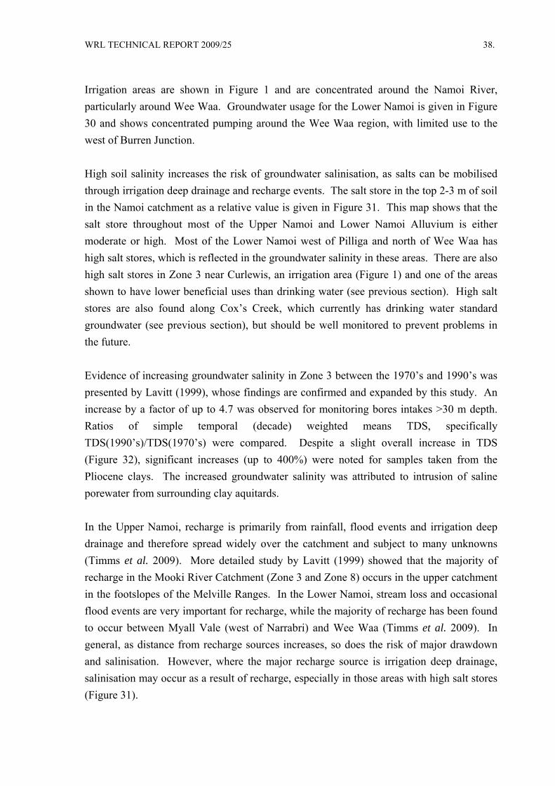
WRL TECHNICAL REPORT 2009/25 38.
Irrigation areas are shown in Figure 1 and are concentrated around the Namoi River,
particularly around Wee Waa. Groundwater usage for the Lower Namoi is given in Figure
30 and shows concentrated pumping around the Wee Waa region, with limited use to the
west of Burren Junction.
High soil salinity increases the risk of groundwater salinisation, as salts can be mobilised
through irrigation deep drainage and recharge events. The salt store in the top 2-3 m of soil
in the Namoi catchment as a relative value is given in Figure 31. This map shows that the
salt store throughout most of the Upper Namoi and Lower Namoi Alluvium is either
moderate or high. Most of the Lower Namoi west of Pilliga and north of Wee Waa has
high salt stores, which is reflected in the groundwater salinity in these areas. There are also
high salt stores in Zone 3 near Curlewis, an irrigation area (Figure 1) and one of the areas
shown to have lower beneficial uses than drinking water (see previous section). High salt
stores are also found along Cox’s Creek, which currently has drinking water standard
groundwater (see previous section), but should be well monitored to prevent problems in
the future.
Evidence of increasing groundwater salinity in Zone 3 between the 1970’s and 1990’s was
presented by Lavitt (1999), whose findings are confirmed and expanded by this study. An
increase by a factor of up to 4.7 was observed for monitoring bores intakes >30 m depth.
Ratios of simple temporal (decade) weighted means TDS, specifically
TDS(1990’s)/TDS(1970’s) were compared. Despite a slight overall increase in TDS
(Figure 32), significant increases (up to 400%) were noted for samples taken from the
Pliocene clays. The increased groundwater salinity was attributed to intrusion of saline
porewater from surrounding clay aquitards.
In the Upper Namoi, recharge is primarily from rainfall, flood events and irrigation deep
drainage and therefore spread widely over the catchment and subject to many unknowns
(Timms et al. 2009). More detailed study by Lavitt (1999) showed that the majority of
recharge in the Mooki River Catchment (Zone 3 and Zone 8) occurs in the upper catchment
in the footslopes of the Melville Ranges. In the Lower Namoi, stream loss and occasional
flood events are very important for recharge, while the majority of recharge has been found
to occur between Myall Vale (west of Narrabri) and Wee Waa (Timms et al. 2009). In
general, as distance from recharge sources increases, so does the risk of major drawdown
and salinisation. However, where the major recharge source is irrigation deep drainage,
salinisation may occur as a result of recharge, especially in those areas with high salt stores
(Figure 31).

WRL TECHNICAL REPORT 2009/25 39.
5.3 Risks Areas in the Namoi Catchment
This section outlines risk areas in the Namoi catchment identified through the analysis of
historical water quality and water level data.
5.3.1 Water Quality
An analysis was completed on the historical water quality data available to compare the
average EC from 1980-1999 to the average EC from 2000-2009, as a way of identifying
possible trends in the data. The results are shown in Figures 33-36.
In the upper monitoring unit, most of the available data is centred around Zone 3 of the
Upper Namoi. Figure 34 (focussed on the Upper Namoi) demonstrates increases in salinity
in the Cox’s Creek catchment (1 data point only) and in Zone 3 of the Upper Namoi. Both
these areas were shown to have high salt stores (Figure 31). The largest increases occur
east of the Namoi River in Zone 3 (average EC from 2000-2009 is 123% greater in
GW036166 than the average from 1980-1999), however, these are intermingled with bores
showing no real increase. In between Curlewis and the Namoi River, all bores showed
some increase over this period (11-25%). It is certainly clear that this area is at major risk
of salinisation.
Less data is available for the upper monitoring unit of the Lower Namoi (Figure 35), which
in general seems to be fairly stable with respect to salinity (where data is available). There
are a few points showing some increase in salinity to the south-east of Wee Waa towards
the edge of the alluvium, and to the west of Burren Junction, towards Pian Creek.
There are not as many data points available in the lower monitoring unit (Figure 36), but
the data available again shows a large area of risk around Zone 3 of the Upper Namoi.
Those areas of Zone 3 showing particular increases in salinity are repeated in the lower
monitoring unit, with the very large increases shown in between Curlewis and the Namoi
River, and west of the Namoi River (GW036166).
An analysis was completed to see if there had been any change in beneficial use between
2000-2005 (as shown in Section 5.1) and 2006-2009. Only 27 bores of the 1268
monitoring bores across the catchment had sufficient data to analyse the beneficial use for
both time periods. Table 16 shows the five bores (seven pipes) with changed beneficial use
category, only one of which has lowered in quality. It is important, however, to note the
resolution of the beneficial use categories (as described in Section 5.1). It still may be that
while the water has remained within the broad beneficial use category of “Irrigation and

WRL TECHNICAL REPORT 2009/25 40.
poultry”, that it is no longer suitable for sunflower and wheat irrigation or poultry watering,
and is only suitable for cotton and barley irrigation.
Table 16 Change of Beneficial Use in the Namoi Catchment
LocCode Monitoring Unit Beneficial Use-2005 Beneficial Use-2009
GW030061 Lower Irrigation and Poultry Drinking
Lower Livestock Irrigation and Poultry GW036166 Upper Livestock Irrigation and Poultry
GW036190 Upper Drinking Irrigation and Poultry
GW036200 Upper Irrigation and Poultry Drinking
Lower Livestock Irrigation and Poultry GW040822 Upper Livestock Irrigation and Poultry
5.3.2 Water Levels
5.3.2.1 Hydrographs
Bores that are representative of groundwater conditions in each zone are shown in Figure
37. Hydrographs from these bores were given in the Upper Namoi Status Report 2004
(DIPNR, 2006) and Lower Namoi Status Report (Smithson, 2009) and have been
reproduced for this report (Figures 38-50) with updated water level information. A
summary of the outcomes from the hydrograph analysis are given in Table 16.
In Zone 1 of the Upper Namoi Alluvium (Borambil Creek, Willow Tree to the Quirindi-
Pine Ridge Road), bores GW030029, GW030024 and GW030184 (Figure 38) can be seen
to have all pipes highly connected. Water levels in these bores can be seen to fluctuate
seasonally with the pumping cycles and have been shown to be strongly influenced by
climate (DIPNR, 2006). Recent groundwater levels in these bores appears to be at or below
the lowest recorded historically.
In Zone 2 of the Upper Namoi Alluvium (Cox’s Creek, Mullaley to Boggabri), there is no
clear correlation with rainfall (DIPNR, 2006). A detailed analysis of hydrographs and 3D
connectivity was recently presented by Kelly (2009). In summary, it was found that
groundwater levels in the semi-confined aquifers have declined by over 10 m over the past
20 years, but that groundwater levels have risen in 14 of the 33 locations. Most of the
locations where groundwater levels are rising are in the unconfined aquifer, where rise may
be a consequence of deep drainage.

WRL TECHNICAL REPORT 2009/25 41.
Hydrographs from representative bores (Figure 39) show poor connection between upper
pipe and lower pipes of each bore, other than for GW036508. Recovered levels in
GW036508 display a continued decline in the recovered head readings. The hydrograph
for GW036515 shows the reversal of hydraulic gradients between the upper and lower
monitoring units after development in 1993, and ongoing decline in recovered water level
heads which is at similar levels to 1997-1998. Record drawdown was recorded in the lower
monitoring unit in 2007 and is greater in this bore than for the other representative bores in
this zone, and a steady decline is seen in the upper monitoring unit, indicating that there
may be some downwards leakage occurring. Similar responses in the upper pipes of bores
GW036546 and GW036600 also indicate leakage from upper monitoring units, increasing
the potential for aquifer compaction.
Recovered levels in bores GW036499 and GW036546 have improved a little since the
worst recoveries recorded in 2004, though drawdowns continue to be of a similar
magnitude. In contrast, recovered water levels in GW036600 and GW036478 are in
continued decline. Record drawdowns were evident in these bores in 2006 and 2007
respectively.
Hydrographs for representative bores in Zone 3 of the Upper Namoi Alluvium (Mooki
Valley - Breeza to Gunnedah) are shown in Figure 40. These hydrographs show varied
connectivity between upper and lower pipes. All pipes in the lower monitoring unit show
declining trends. Current recovery levels in the lower monitoring units of GW036152 and
GW036190 are the worst on record, while recoveries in GW036097, GW036189 and
GW036215 were worst around 2002 - 2003, but have improved very little since then.
Certainly, since 2002-2003, there is a noticeable stepdown in recovery in all of the bores.
Pipe 1 of GW036189 indicates there is dewatering occurring. There is a risk of compaction
and loss of storage throughout the zone.
Hydrographs for representative bores in Zone 4 of the Upper Namoi Alluvium (Namoi
Valley - Carroll Gap to Boggabri) are shown in Figure 41. Decline of recovered water
levels is evident in all bores. GW030306 and GW030344 display the most evidence of
pumping impacts with large seasonal drawdowns and increasing hydrograph separation
between pipes over time, which may increase the potential for downward leakage. Water
level recovery in these bores was the lowest recorded during 2006 and 2007 respectively.
Recovered water levels during 2007 were also the lowest recorded for GW021093,
GW036485, GW036513 and GW036007. Steps down in water level recovery are evident
in most of these hydrographs for the major droughts of the early 1980’s, mid 1990’s and
2002/2003; no complete recovery to pre-drought levels were made after these steps.

WRL TECHNICAL REPORT 2009/25 42.
Hydrographs for representative bores for Zone 5 of the Upper Namoi Alluvium (Namoi
Valley - Boggabri to Narrabri) and Zone 11 (Maules Creek) are shown in Figures 42 and
43. Pumping impacts in Zone 5 are seen most clearly with seasonal drawdowns in bores
GW036016, GW036005 and GW030233. GW030478, located in the downstream end of
Zone 5 shows less seasonal pumping impact, but can also seen to be in a slight decline over
time. There is some evidence of decline in these bores with recent recovered water levels
the lowest on record. Pipe 1 in GW036005 became dewatered in 2007, and there is an
upward hydraulic gradient in this location when water levels are recovered. Bores
GW030129 and GW030132 are located close to Maules Creek in Zone 11, while
GW030237 is located further from the creek in Zone 11, however all of the bores have
maintained fairly stable water levels over time. Due to the similar patterns of extraction
and recovery in Bore GW030233 (Zone 5) and GW030235 (Zone 11), DIPNR (2006)
suggested that there was evidence that pumping in Zone 5 was impacting on Zone 11.
Representative hydrographs for bores in Zone 6 of the Upper Namoi Alluvium (Mooki
Valley - tributaries of the Liverpool Range) and Zone 10 (Warrah Creek) are shown in
Figure 44. Pumping impacts can be seen in GW030147 (in the north-west of Zone 6), with
recovery levels depressed since 2002, while groundwater fluctuates with river levels in
GW030141 (located on the Mooki River) and appears relatively stable over time.
GW030176 (east of the Mooki River) is not showing climatic or extraction impacts,
however, the upwards hydraulic gradient between the two pipes has reduced over time.
GW030181 represents the seasonal fluctuations of the groundwater (DIPNR, 2006).
GW030060 is the most impacted by pumping of the representative monitoring bores, with
large seasonal drawdowns. The lowest recovered heads were seen in the mid 1990’s and
2003; since this time recovered heads have been increasing. GW030059 is the only
hydrograph shown for Zone 10 and is stable over time.
Representative hydrographs for bores in Zone 7 of the Upper Namoi Alluvium (Yarraman
Creek) are found in Figure 45, however only one bore has data prior to 2001. Recovery has
been improving in GW093101 and GW965576 since the lowest drawdown in 2003.
Recovery in bore GW093103 was slower after 2003 than the recovery in the previous two
bores, however, the bore has recovered to 2001 levels. This bore shows significant
seasonal drawdown. Bore 036099 is the only one in Zone 7 with a long historical data set
and is in the downstream end of the zone. Water levels are reasonably well correlated with
rainfall (DIPNR, 2006). Hydrograph separation between the pipes was evident between
2001-2006, with Pipe 2 in the lower monitoring unit showing the impact of the extraction
during this dry period. The hydraulic gradient between these pipes has reversed in periods
of increased extraction, however, the bore has been recovering slowly since the record

WRL TECHNICAL REPORT 2009/25 43.
drawdown in 2003, and is close to 2001 recovery levels again, though there does seem to be
some decline in recovery since the late 1990’s. Bores GW093105 and GW093106 even
further downstream than GW036099 are located close to the boundary of Zone 8. While
water levels in GW093105 have been relatively stable, there has been some decline in
recovery in GW093106 in response to pumping.
Representative hydrographs for Zone 8 of the Upper Namoi Alluvium (Mooki Valley –
Quirindi-Pine Ridge Road to Breeza) are found in Figure 46. Declining recovery is evident
in all bores, with recovery at or equal to record lows in all bores. Step downs in recovery
levels can be seen to correspond to periods of low rainfall, however, water levels have not
recovered to previous levels prior to the droughts. This indicates that usage during wetter
periods may be equal to recharge, while during dry periods extraction is draining storage.
The declining trend is least regular in bore GW030087 at the upstream end of the zone,
close to Quirindi Creek. This bore has been shown to have strong correlation with rainfall
trends. Pipe 1 of GW030012 was dewatered in 2003 and has not recovered since.
Representative hydrographs for Zone 9 of the Upper Namoi Alluvium (Cox’s Creek –
Upstream of Mullaley) are found in Figure 47. These bores have been shown to be strongly
influenced by climate (DIPNR 2006). The influence of extraction is seen in bore
GW036601 after the mid 1990’s. There may be some slight decline in this bore.
Representative hydrographs for Zone 12 of the Upper Namoi Alluvium (Kelvin Valley) are
found in Figure 48. Recharge in this zone is likely to be from the basement rock, rather
than from surface infiltration (DIPNR, 2006), with groundwater flowing through to Zone 4.
A rising trend is seen in the hydrographs for GW036432, GW036418 and GW036322
(located in the downstream end of the catchment) prior to 1994, after which point the
impact of extraction can be seen. Since this time there has been a declining trend in the
hydrographs. In GW036418, the upper aquifer has become unconfined. GW036307 and
GW036415 are located in the centre of Zone 12 and show an upwards leakage potential.
These bores both show dewatering occurring in the upper monitoring unit.

WRL TECHNICAL REPORT 2009/25 44.
Table 16 Summary of Hydrograph Analysis for the Upper and Lower Namoi Alluvium
GMU Zone Summary of Hydrograph Analysis
1 Current recovery poor, in need of major recharge event.
2 Record drawdowns and decline in water levels. Strong evidence of leakage from upper monitoring unit to lower monitoring unit.
3 Most bores in significant decline, with a stepdown in recovery evident since 2002-2003. Rising groundwater levels are evident on the eastern edge of Zone 3, and some bores where groundwater had been drawdown have shown some recovery recently.
4 Some decline evident in all bores, except a site east of Boggabri with rising groundwater level.
5 and 11 Decline evident in some bores, particularly in Zone 5, with pumping in Zone 5 showing some impacts on Zone 11.
6 and 10 Groundwater head response are variable.
7 Some slight decline in recovery evident in some bores closeto the boundary with Zone 8.
8 Significant decline shown throughout the zone with stepsdown in recovery during dry periods.
9 Groundwater head response are variable.
Upper Namoi
12 Water levels in decline throughout the zone.
Lower Namoi Large drawdowns, with areas of greatest decline (recovered levels) between Narrabri and Wee Waa to the north of the Namoi River. Groundwater level in most bores is in decline. A few bores on the southern edge of the Lower Namoi showincreased groundwater levels.
Representative hydrographs for the Lower Namoi Alluvium are shown in Figures 49-50,
with locations of representative bores found in Figure 37. This analysis of hydrographs is a
summary of the findings of the recently released Lower Namoi Groundwater Status Report
(Smithson, 2009). GW030310 is located between Narrabri and Wee Waa and shows
recovery decline of 4.3 m since development and decreasing pressure difference between
pipes.

WRL TECHNICAL REPORT 2009/25 45.
Large drawdowns are shown in GW021266 (north-east of Wee Waa), especially in the
deeper monitoring unit. A reversal of hydraulic gradient between the monitoring units
occurred around 1980, such that the head of the deeper aquifer is now approximately 9 m
lower than that of the shallower monitoring unit. It is possible that these differences are
due to measurement, however, there is certainly a head reversal occurring between pipe 3
and pipe 4. The hydrograph for GW030238 is located to the west of GW021266, north-east
of Wee Waa, however, all pipes in this location show good hydraulic connection, yet also
demonstrate very large drawdowns (~39 m). Both of these bores are showing declining
water level recovery over time, especially in the deeper monitoring unit.
GW030238 is located to the far north of Wee Waa and is demonstrating significant water
level recovery decline (28.5 m), as is GW025299, located to the north-west (11.6 m).
GW025045 is to the south of this bore and screened in the upper and lower monitoring
units. Decline in water levels in the lower monitoring unit is inducing leakage from the
upper monitoring unit, and both are showing declining recovery in water levels. Bores
GW036045 and GW025245 are located along a section to the south of GW025299 and are
exhibiting similar hydrograph separation and decline in water level recovery in the lower
monitoring unit. GW025141 is further to the south of these bores on the same section.
Water levels in the pipes are in poor hydraulic connection but declining water level
recovery in the lower monitoring unit (11 m) is inducing leakage and corresponding water
level decline in the upper monitoring unit; this pipe has been dewatered since 2005.
GW036255 is located to the west of the management area, in the far north above Burren
Junction, where all pipes are in relatively good hydraulic connection, however hydrograph
separation has been increasing with development. Water level recovery decline appears to
have recovered since the mid 1990’s. GW036249 is located close to Burren Junction and is
showing very slight recovery decline over time. GW036320 is the furthest west of the
representative monitoring bores, located to the east of Cryon. There is hydraulic separation
between an upper and deeper monitoring unit, with the deeper unit showing recovery
decline of ~9 m.
5.3.2.2 Historical Water Level Variation
Maps of change in water level recovery are shown in Figures 51 – 641. The maps have
been divided into time intervals based around the key date of 2006, as the catchment
management targets require either stability or improvements from 2006. The first series of
maps (Figures 51 – 58) shows the change in water level recovery prior to 2006, with the 1 Raster interpolation of the water level data was completed using the Inverse Distance Weighted Method in ArcGIS with a fixed radius of 3, power of 2 and a minimum number of 1 point

WRL TECHNICAL REPORT 2009/25 46.
majority of maps comparing the 1978 levels to 2006 levels. As there were no monitoring
bores in Cox’s Creek at this time, another map has been generated for the Upper Namoi
comparing 1988 levels to 2006 levels (though it should be noted that data is still only
available for the downstream end of Cox’s Creek. The second series of maps (Figures 59-
64) show the change in water level recovery for 2006 to 2008.
The change in water level recovery for the upper monitoring unit of the Upper Namoi is
shown in Figure 51, while Figure 52 shows Zone 3 of the Upper Namoi at higher
resolution. While these figures show some water level recovery decline from 1978 – 2006
across most of the Upper Namoi, the most affected area is clearly Zone 3 (up to 15 m
decline in water level recovery), with Zone 8 also showing significant decline (up to 13 m).
This map can be compared with Figure 54, which shows the water level recovery decline
from 1988 – 2006. Over this period, significant decline can still be seen in Zone 3 and also
in Zone 12, where much of the development appears to have occurred during the early
1990’s.
The change in water level recovery for the upper monitoring unit of the Lower Namoi is
shown in Figure 53. The area of greatest water level recovery decline can be seen on the
north-south section around Wee Waa, with the greatest decline across the whole catchment
found on the alluvial boundary to the far-north of Wee Waa.
Less data is available for the lower monitoring unit of the Upper and Lower Alluvium. It is
therefore important to be aware of the location of actual data points, rather than simply
observing the colours of the contouring on the map. Figure 55 shows the change in water
level recovery for the lower monitoring unit of the Upper Namoi, while Figure 56 shows
Zone 3 of the Upper Namoi at higher resolution. The available data again shows Zone 3
and Zone 8 to be the areas of greatest water level recovery decline. Where the data is
available in Zone 3 (compare Figure 52 to Figure 56), it appears that the drawdown is
greater in the lower monitoring unit, indicating that extraction in the lower monitoring unit
may be causing leakage from the upper monitoring unit.
The change in water level recovery for the lower monitoring unit of the Lower Namoi is
shown in Figure 57. The area of most decline is again seen in the section around Wee Waa,
with the greatest drawdown in to the south-east of Wee Waa. The only monitoring bore
shown to be intersecting the lower monitoring unit in the far north section is not showing
decline (compare with Figure 53), however Figure 53 does show that the areas of decline in
the Lower Namoi are very localised.

WRL TECHNICAL REPORT 2009/25 47.
Figures 59 – 64 show the change in water level recovery from 2006 – 2008. These maps
show that there has been little decline in the seasonal water level recovery point in the
upper or lower monitoring units of the Upper Namoi during this time. A few isolated
patches of decline can be seen in Zone 3 (Figure 60). In comparison, water level recovery
decline has been much more widespread in the Lower Namoi, with the region around Wee
Waa showing mostly 2 -3 m water level recovery decline in the upper monitoring unit
(Figure 61). While there is less data in the lower monitoring unit, it seems that the decline
is even more widespread.
In areas of extreme water level recovery decline coupled with clay soils, there is a risk of
consolidation of sediments. Hydrographs from bores with more than 20 m water level
recovery decline between 1978-2006, 10 m between 1988-2006 and 5 m from 2006-2008
were examined in more detail to determine whether the decline might pose a genuine risk of
consolidation. Bores identified in this analysis that may need further investigation in the
future are summarised in Table 17.
Table 17
Bores with Decline of Recovered Levels Indicating Possible Risk of Consolidation
Bore No. Pipe Start Year
End Year Final SWL (m)
Average Screen Depth (m)
Decline of recovered levels
(m) GW025054 2 1978 2006 46.5 102.77 -20.49 GW025055 3 48.05 98.08 -20.62 GW030222 1 52.18 108.19 -20.08 GW030222 2 52.36 97.63 -20.36 GW030223 2 52.06 78.64 -20.11 GW036045 3 1988 2006 46.63 62.2 -11.55 GW036149 1 23.35 220.19 -11.95 GW036149 2 24.5 208.04 -13.15 GW036149 3 27.8 169.99 -15 GW036149 4 26.51 145.33 -13.39 GW036150 1 25 206.87 -14.15 GW036151 2 25.38 185.94 -14.26 GW036166 2 25.65 194.78 -14.67 GW036166 3 25.44 176.47 -14.39 GW036167 2 21.12 232.03 -10.5 GW036167 3 26.1 198.54 -14.63 GW036193 3 27.38 150.81 -13.58 GW036215 2 22.32 201.67 -11.56 GW036215 3 22.4 177.67 -11.52 GW036266 1 19.65 250.7 -10.75 GW036266 3 19.73 158.4 -10.3

WRL TECHNICAL REPORT 2009/25 48.
5.3.3 Combined Risks
The major risk area identified both in terms of water quality and water level pressures is
Zone 3 of the Upper Namoi, which is experiencing both significant increases in salinity and
long term decline in water levels. Comparing Figures 34, 36 and Figure 52, it is evident
that the areas of greatest salinity increase coincide with those areas of greatest drawdown.
Historical water level has been compared with salinity for several bores within Zone 3 and
are shown in Figures 65 – 67. All of these bores are WRL target bores and can be found in
Figure 5, with the exception of GW036213, which is located on the western side of the
Mooki River just to the north-east of GW036210.
At site GW036213 (Figure 65) sharp increases in salinity occurred above 40 m occurring
from 2002, corresponding to a distinct decline in water level in the lower pipes during the
drought at that time. At GW036151 (Figure 65) there was a peak in salinity in Pipe 1 (~40
m depth) at the same time (around 2002), which also corresponds to a distinct water level
recovery decline. After this time, water levels appear to stabilise at this new level and
salinity starts to decline again. Bore GW036166 (Figure 66) shows a similar pattern of
increase in Pipe 1 (~47 m depth). Although there are not as many data points to determine
the time of increase, it does seem that it may have followed a similar pattern to GW036213
and GW036151. Pipe 2 (79 m) has also increased salinity significantly; water from Pipe 1
and Pipe 2 is no longer suitable for cotton irrigation (7,700 μS/cm). GW036190 is again
similar to the other 3 bores examined. Salinity increase in Pipe 1 (32 m depth) appears to
correlate with the water level recovery decline around the year 2001-2002, and then
stabilises. This pattern seems to indicate that salinity increases in this area may be
associated particularly with periods of large extraction during drought periods, although
there is not enough salinity data to confirm this.
GW036200 (Figure 67) is located further away from the river on the edge of the alluvium
and is showing significantly different trends. Water levels have an overall rising trend in
all pipes (~87 m and above), although water levels have been in decline since 2000.
Salinity has been increasing at depth, however, while salinity increased prior to 2002 in
Pipe 2 (~44 m depth) it has since decreased. The period of increasing salinity appears to be
associated with increasing water levels. Water levels in this bore does not show any strong
pumping influence.
Based on decline in water level recovery, there may also be significant risk in Zone 8 of the
Upper Namoi, and north of Wee Waa in the Lower Namoi, however, no corresponding
historical groundwater salinity data was available to compare. Soil salinity (Figure 31) in
the area of drawdown in Zone 8 (Figure 51) is moderate, while soil salinity in the majority

WRL TECHNICAL REPORT 2009/25 49.
of the Lower Namoi is high and therefore both areas appear to be at risk from salinisation.
The Lower Namoi around Wee Waa appears to be at increased risk due to the greater
intensity of irrigation in that area (Figure 30).
In summary, based on available information, the areas of groundwater resources that are
considered to be at risk are:
Upper Namoi – Zone 3 due to groundwater salinity and levels
Upper Namoi – Zone 8 due to groundwater levels and moderate soil salinity
Lower Namoi – north of Wee Waa due to groundwater levels and high soil salinity
Lower Namoi – across GWMA, due to high soil salinity and near Wee Waa the greater
intensity of irrigation.
5.4 Recommendations for Future Surveys
Based on the analysis of risks in the catchment, future surveys could be beneficially
expanded in several ways:
A further round of groundwater sampling of monitoring bores should be completed over
the growing season (periods of high and low stress) to determine if there are definite
trends in water quality response to a pumping season (see Section 4.2.2.3)
Further analysis and verification of the connectivity method should be completed and
more pipes intersecting the lower monitoring unit should be selected for ongoing
monitoring
Monitoring density should be increased in areas of high risk that are currently poorly
covered i.e. Zone 8 of the Upper Namoi, and the Lower Namoi to the north of Wee
Waa.
Ideally, future surveys would also be expanded to include additional GWMA’s not
currently included in the survey (eg. fractured rock areas).
These recommendations are incorporated in the strategic monitoring plan in Section 6.

WRL TECHNICAL REPORT 2009/25 50.
6. STRATEGIES FOR BEST PRACTICE GROUNDWATER MONITORING
This section aims to outline guidelines for a best practice monitoring strategy to improve
assessments and best management responses to groundwater conditions. Standard
monitoring guidelines currently applied in Australia and the MDB have been tailored for
the Namoi catchment by identifying a series of triggers that will identify adverse risks and
will involve irrigators and the community. These guidelines address both the practicalities
and expense of obtaining groundwater data and the quantitative evaluation of monitoring
data to identify risks and provide early warning of the degradation of the resource.
Information regarding the availability of monitoring data and general information about
groundwater monitoring framework design were found in Timms et al. (2009). This
section gives more specific recommendations for continuing and improving this monitoring
program.
6.1 Groundwater Monitoring Strategy Concepts
6.1.1 Levels of Best Management Practice
The Cotton CRC is currently redefining best management practices for the cotton industry
in Australia: myBMP; a web-based system to provide scientific information and assessment
tools to growers, is in the final stages of development (S. Higgins, pers.com). This system
is based on four levels of progress as outlined below:
Level 1 Practices are legal requirements and industry protocols
Level 2 Practices are considered practices growers should be adopting as a minimum
and is certification standard for the cotton industry
Level 3 Practices are considered above standard, and ones growers should be working
towards achieving
Level 4 Is aspirational.
This BMP system includes worksheets designed for individual growers to rate and
benchmark their own farming practices and includes components relevant to groundwater
monitoring. However, best management practice for groundwater monitoring is needed not
only at individual farming scales in the Namoi catchment but also at regional, subcatchment
and community scales. The concept of progress levels used by the Cotton CRC can be
usefully adopted for this larger scale groundwater monitoring program, to complement
those being created for individual growers. This recognises achieving best management

WRL TECHNICAL REPORT 2009/25 51.
practices may take time, and may be challenging within current budgetary constraints, yet
useful steps can be taken along the path to achieving the highest level of best management
practice.
6.1.2 Purpose of Groundwater Monitoring
It is important to identify the purpose(s) for groundwater monitoring. An effective
groundwater monitoring program is designed to satisfy the purposes intended for the data,
and is practically achievable within the available funding, personnel and equipment. The
purpose of the groundwater monitoring program influences the frequency and duration of
monitoring, sampling and the analysis of data.
6.1.3 Frequency and Duration of Monitoring for Various Purposes
The frequency and duration of groundwater monitoring is dependent on the issues being
examined (i.e. the purpose) and the response of the groundwater system to change. The
frequency of monitoring may also depend on the stage of a project and environmental
assessment requirements. For example, monitoring should be designed specifically for:
establishing baseline water quality and on-going monitoring of significantly changed land
use where groundwater contamination is a possibility.
Duration, and continuity of monitoring is equally important to the frequency of monitoring,
although most groundwater quality monitoring is limited to a short period.
6.1.4 Sampling
Groundwater sampling and analysis is expensive and needs to be undertaken strategically to
fit the purpose of monitoring. The cost of acquiring a sample will be affected by the
distance between bores and accessibility of the bores, purge time required prior to sampling
and the cost of laboratory analyses to be completed. As much of the cost of the sample will
be within the actual labour time required to collect the sample, it may be more efficient and
beneficial in the long run to perform more analyses on the samples; however a trade-off is
required between the number of bores that can be sampled and the analyses that are
performed.
Analysis must be completed by laboratories that are NATA registered for the analyses
being conducted. Standard sampling procedures must be used to ensure the integrity of the
data (see Appendix A3).

WRL TECHNICAL REPORT 2009/25 52.
6.1.5 Data Analysis
Appropriate analysis of data is crucial to the effectiveness of any monitoring program.
Data must be comparable in terms of locations and parameters, so that any changes within a
system over time can be determined. Any triggers adopted must be meaningful within the
context of available (often limited) data. It is difficult to parameterise baseline conditions
with confidence in a groundwater catchment setting over such a large heterogeneous area,
and therefore is often only possible to try and determine if there is an ongoing trend in the
data and whether that trend is significant.
6.2 Catchment Scale Groundwater Monitoring
This project has helped to more clearly identify areas of risk in the Upper and Lower
Namoi Alluvium of the Namoi catchment in terms of water levels and salinity and to
identify knowledge gaps in the Namoi catchment. Based on this information, catchment
scale groundwater monitoring needs to be reviewed and adapted to suit the ongoing needs
for information about catchment conditions. This section gives recommendations for
ongoing best practice groundwater monitoring for the Namoi catchment. Best practice
groundwater monitoring is outlined for three progress levels of monitoring relevant to the
purposes of monitoring defined in the next subsection.
6.2.1 Purpose of Monitoring
This project is directly addressing data gaps for groundwater level and groundwater quality
that were identified in Timms et al. (2009).
The primary purposes of this groundwater monitoring program are:
Detect changes in groundwater levels and salinity
Determine if changes are significant to beneficial use of groundwater
Establish groundwater benchmark and trigger values for action
Assess the response of extraction
Identify “hotspot” areas that are sensitive to impacts.
This monitoring program would need to be reviewed and updated, should any other
purposes be added to this list.

WRL TECHNICAL REPORT 2009/25 53.
6.2.2 Data Report Card Across the Catchment
A basic report card of data availability for each GWMA based on analysis of the database
developed by WRL is given in Table 18. Given the significance of the resource, there has
been very little collection of water quality data in the Lower Namoi Alluvium. This table
suggests that nutrient and agrichemical data collection is sparse across the catchment. This
has been used to inform the levels of best practice monitoring identified for site selection
and parameters in particular.

WRL TECHNICAL REPORT 2009/25 54.
Table 18 Water Quality Data Availability from Monitoring Bores across the Namoi Catchment
EC Major Ions1 Agrichemicals2 Nutrients3 Total No. Bores
GMU Zon
e
No. Data Points
No. Bores
No. Data Points
No. Bores
No. Data Points
No. Bores
No. Data Points
No. Bores
Monitoring*
Production#
Ratio^
N01 Lower Namoi Alluvium 503 22 424 22 1 1 1 1 443 868 2
N04 Upper Namoi Alluvium 1 191 31 211 29 3 3 3 3 14 73 5.2
N04 Upper Namoi Alluvium 2 247 107 223 98 14 9 14 5 75 138 1.8
N04 Upper Namoi Alluvium 3 1332 176 1288 160 23 13 131 53 107 295 2.8
N04 Upper Namoi Alluvium 4 823 221 751 189 26 19 49 37 128 465 3.6
N04 Upper Namoi Alluvium 5 670 95 591 92 2 2 3 2 76 197 2.6
N04 Upper Namoi Alluvium 6 315 52 298 39 15 7 13 7 27 105 3.9
N04 Upper Namoi Alluvium 7 31 19 24 14 - - - - 19 50 2.6
N04 Upper Namoi Alluvium 8 893 117 843 107 6 6 6 6 68 208 3.1
N04 Upper Namoi Alluvium 9 62 39 53 30 7 6 11 6 35 85 2.4
N04 Upper Namoi Alluvium 10 - - - - - - - - - -
N04 Upper Namoi Alluvium 11 154 27 155 28 - - - - 16 55 3.4
N04 Upper Namoi Alluvium 12 81 13 75 9 - - - - 19 46 2.4
N05 Peel Valley Alluvium 243 149 231 142 - - 18 8 58 653 11.3 N23 Miscellaneous Alluvium of the Barwon Region 55 47 65 49 - - - - 7 127 18.1
N601 GAB Intake Beds 138 94 162 103 - - - - 13 80 6.2
N604 Gunnedah Basin 263 182 240 168 2 2 4 4 25 96 3.8
N608 Oxley Basin 235 144 163 110 16 7 24 10 34 124 3.6
N63 GAB Alluvial 122 31 124 32 1 1 1 1 4 7 1.8
N805 New England Fold Belt 151 102 154 99 - - 1 1 17 139 8.2 N813 Warrumbungle Tertiary Basalt 1 1 1 1 - - - - - -
N814 Liverpool Ranges Basalt 253 214 26 23 6 3 6 3 7 31 4.4 N819 Peel Valley Fractured Rock - - 192 150 - - 2 2 76 408 5.4
Total 6763 1883 6294 1694 122 79 287 149 1268 4250

WRL TECHNICAL REPORT 2009/25 55.
* Monitoring bores include groundwater exploration bores from DWE registered bore database. The current status of these monitoring bores is unknown. A proportion of these monitoring bores may be currently monitored. Some bores may not be accessible, or have corroded, collapsed, silted intake screens or otherwise unsuitable to provide useful data. # Production bores include irrigation and town water supply from DWE registered bore database. ^ Ratio of production bores to monitoring bores. 1 Calcium used as reference parameter to infer collection of major ion dataset 2 Atrazine used as reference parameter to infer collection of agrichemical dataset 3 Nitrate as N used as reference parameter to infer collection of nutrient dataset
6.2.3 Site Selection
Criteria for selecting representative bores for sampling in this project included the
following:
Areas where a change in water quality would increase the risk of change in beneficial
use class
Coverage of groundwater management zones
Data availability from previous monitoring
Proximity to major groundwater extraction
Proximity to river recharge sources
Groundwater quality changes identified
Proximity to significant salt sources.
Results of this sampling project indicate that this set of representative bores should be
expanded according the following criteria:
Further analysis and verification of the connectivity method should be completed and
more pipes intersecting the lower monitoring unit should be selected for ongoing
monitoring
Monitoring density should be increased in areas of high risk that are currently poorly
covered i.e. Zone 8 of the Upper Namoi, and the Lower Namoi to the north of Wee
Waa.
Ideally, future surveys would also be expanded to include additional GWMA’s not
currently included in the survey (eg. fractured rock areas).
Those bores used as representative bores for groundwater resource status updates (see
Section 4.2.2.1) should be considered first for inclusion into the future groundwater
monitoring program.

WRL TECHNICAL REPORT 2009/25 56.
Table 20 What Sites Should be Monitored in the Namoi Catchment for BMP
Groundwater Monitoring?
Monitoring
Level
Practice
Basic Representative bores for groundwater level every ~6 weeks and
significant sites with continuous telemetry monitoring.
Groundwater salinity monitoring* several times per year at a limited
number of bores in zones.
Moderate As above plus:
Additional representative bores with continuous telemetry
monitoring
Groundwater salinity monitoring at the start of each irrigation
season (annual) in representative bores in all GWMAs/zones
identified at risk of groundwater salinisation i.e. Zone 3 and
Zone 8 of Upper Namoi, and Lower Namoi to north of Wee Waa
High ** As above plus:
Groundwater salinity monitoring at the start of each irrigation
season (annual) in bores that have been monitored in this project
(covers most but not all alluvial GWMAs) with addition of bores
in areas of high risk and greater coverage in lower monitoring unit.
Install additional monitoring bores in GWMAs that are currently
not monitored for groundwater level or salinity.# * Groundwater salinity at monitoring bores should include on-site measurement of basic field parameters including EC, pH and temperature, and laboratory analysis of major ions. Automated monitoring of EC is not possible in monitoring bores due to stagnant water. ** Berhane & Tennakoon (2003) recommended that approximately 10% of monitoring sites in the Barwon Region should be selected for a primary monitoring network of groundwater quality to allow analysis of long term groundwater quality trends. # Monitoring bore coverage analysis, as indicated by the ratio of production bores to monitoring bores suggests that additional monitoring points may be required in the Peel Valley (both alluvium and fractured rock areas), the New England Fold Belt, GAB Intake Beds and the Miscellaneous Alluvium of the Barwon Region (see Timms et al. 2009).
In addition to bores sampled for this groundwater monitoring program, groundwater
samples are also currently being obtained for other specific projects in the Namoi
catchment. Rather than duplicating efforts, agreements should be made where possible to
access data from other projects and incorporate them into this monitoring program. These
projects include, but are not limited to:
Monitoring of groundwater salinity below the Cryon Plains by DECCW.

WRL TECHNICAL REPORT 2009/25 57.
Research investigations in the Maules Creek area by UNSW Connected Waters
Initiative.
Research investigations in the Cockburn Creek area by Cook et al. (2007).
Coal and gas exploration and monitoring programs in various areas.
6.2.4 Parameters
The parameters that should be monitored in the Namoi catchment for BMP groundwater
monitoring are outlined in Table 19.
Table 19
What Parameters Should be Monitored in the Namoi Catchment for BMP Groundwater Monitoring?
Monitoring Level
Practice
Basic Groundwater Level Groundwater salinity including on-site measurement of basic field parameters including EC, pH and temperature
Moderate As above plus: laboratory analysis of major ions
High As above plus: periodic laboratory analysis for nutrients and agrichemicals
The monitoring level of parameters may be varied according to the frequency of monitoring
at one site. For example, in areas of High frequency monitoring, a High level of parameters
monitoring may only be appropriate once a year, Moderate four times a year, and Basic for
the remainder of the monitoring events.
6.2.5 Frequency of Monitoring
A basic indication of how frequently water level and water quality parameters should be
measured is given in Table 20 and Table 21. It would be valuable to complete a further
round of groundwater sampling of representative monitoring bores over the growing season
(periods of high and low stress) to determine if there are definite trends in water quality
response to a pumping season (see Section 4.2.2.3).
The frequency of monitoring required may be varied for selected sites and parameters. It
may be appropriate to apply Basic frequency of groundwater quality monitoring in low risk
areas with a Moderate level of parameters, and Moderate frequency in hotspot areas with a
Moderate level of parameters.

WRL TECHNICAL REPORT 2009/25 58.
Table 20 How Frequently Should Water Level be Monitored in the Namoi Catchment
for BMP Groundwater Monitoring?
Monitoring Level
Practice
Basic Quarterly
Moderate 6 weekly
High 6 weekly at sites requiring basic resource monitoring
Daily readings at sites with risk of groundwater quality impacts and
significant drawdowns
Table 21
How Frequently Should Water Quality Parameters be Monitored in the Namoi Catchment for BMP Groundwater Monitoring?
Monitoring Level
Practice
Basic Annual
Moderate Twice per year or Quarterly*
High Monthly * Quarterly allows examination of trends in water quality response to a pumping season and better definition of baseline trends.
This monitoring is considered basic resource monitoring and therefore needs to be ongoing
for as long as the groundwater resource is utilised.
6.2.6 Sampling
Standard sampling procedures must be used to ensure the integrity of the data (see
Appendix A3). This includes purging of bores prior to sampling or use of appropriate low
flow sampling techniques. Analysis must be completed by laboratories that are NATA
registered for the analyses being conducted. It is not considered appropriate to have levels
of best management practice for sampling techniques as the value of data collected will be
compromised by lower standards.
6.2.7 Data Analysis
As the Catchment Target for Surface and Ground Water Ecosystems (see Section 2.1)
requires an “improvement in the condition of surface and ground water ecosystems” from
2006, future data analysis should use the data prior to 2006 as the reference point for
establishing catchment baselines.

WRL TECHNICAL REPORT 2009/25 59.
The following analysis, completed in this report, are considered basic to understanding the
status of the resource and can be completed if a Basic monitoring level is conducted:
Hydrograph plotting and analysis
Mapping of change in recovery levels from 2006
Plotting of historical EC.
A Moderate and High level of site selection for water quality monitoring will also allow the
following to be completed:
Mapping of change in EC from 2006.
Appropriate data analysis is dependant on the monitoring level adopted. The frequency of
monitoring and parameters selected will impact on the analysis that can be completed.
6.2.8 Database Development and Accessibility
WRL has developed two databases (one for water quality and one for water levels) for the
Namoi catchment in MS ACCESS, with pre and post processing of data using Python
scripts and quality checking and correcting where possible. All data and information
obtained during the project has been provided with this report in an appropriate digital
format for upload into public information systems maintained by the Namoi CMA and
DWE.
All future monitoring data must continue to be included in these databases with appropriate
quality control and checking. Of vital importance is the need to be consistent with
terminology and formatting, in particular the need to associate data with the correct
Location Codes and Well Codes. A detailed description of the database standards and
guidelines is given in Appendix A10.
6.3 Grower Groundwater Monitoring
As indicated by the GHD Hassall grower survey, there are a range of opinions as to the
value of community groundwater monitoring. Community monitoring is the aggregation of
sample data from a number of grower bores around the catchment. The samples may be
collected either by the growers, or by an independent team that uses standard protocols to
collect samples. The WRL team considers that community monitoring is of limited value
in a scientific context but that such a program may contribute to greater community
appreciation of groundwater status. One reason for this position is the difference in

WRL TECHNICAL REPORT 2009/25 60.
monitoring bore and irrigation bore design (Figure 68). As irrigation bores may be
screened across several monitoring units, they only give a mixed sample; often the screen
depths are not even known.
As described in the GHD Hassall report, a number of monitoring options were presented at
community groundwater workshops:
1. Enhanced data gathering and communication by DECCW
2. Supplement with additional independent data gathering
• from monitoring bores and / or from grower pump bores
3. Supplement with monitoring by groundwater users of grower pump bores
4. Supplement with independent analysis/ communication
5. No change.
A BMP for groundwater quality monitoring of an irrigation bore has been developed by
WRL for inclusion into ‘myBMP’ (see Section 6.1.1) so that growers are able to monitor
groundwater levels and groundwater quality at a target level. This is shown in the
following box.

WRL TECHNICAL REPORT 2009/25 61.
IRRIGATION BORE BMP WORKSHEET
Level 1 Provide a water quality report in accordance with Departmental approval for water supply
work1 Bore construction and abandonment of old bores in accordance with Departmental bore
licence2 and guidelines for Australia3
Level 2 To maximise yields from crops, use bore water for irrigation within appropriate guidelines4
for salinity (EC). Mix with alternative water sources where appropriate and available. Measure water level and groundwater salinity (EC or electrical conductivity) at the start
and end of each irrigation season using minimum standard methods5 Record ground water level and groundwater salinity for detection of potential trends over
time
Level 3 To maximise irrigation yields use bore water within appropriate guidelines6 for specific
ions, hardness and sodium adsorption ratio. Mix with alternative water sources where appropriate and available.
Continuous measurement using a automated logger for bore water level and quality (EC) Collect samples at the start of each irrigation season for laboratory analysis7 of groundwater
salinity and major ions by following standard methods8 Laboratory testing of major water quality characteristics and comparison with guidelines
for irrigation use (Major ions – sodium, magnesium, potassium, calcium, chloride, sulfate and alkalinity)
Level 4 Continuous sampling using an automated logger for bore water level and quality (EC) with
telemetry to office and/or website. Laboratory testing at the start of each irrigation season of groundwater samples for
nutrients (nitrate and phosphate) and agrichemicals (eg atrazine). Adoption of advanced guidelines9 for bore construction with monitoring access (Resource
fact sheets -include water level dip tubes and sampling tap in bore design) 1 The water supply approval holder is to provide a standard report on water quality as requested by DECCW. Contact DECCW water licensing for advice on 1800 353 104 or www.water.nsw.gov.au and search “water licensing enquiries” and “groundwater licences frequently asked questions” 2 Contact DECCW water licensing for advice on 1800 353 104 or www.water.nsw.gov.au and search “water licensing enquiries” and “groundwater licences frequently asked questions” 3 “Minimum Construction Requirements for Water Bores in Australia” is available for download at www.water.nsw.gov.au and search for “Driller’s licences” 4 See Table 1 of this report 5 Minimum standard methods include purging stagnant water from the bore casing for 15 minutes and calibration of EC meter. See Fact Sheet “DIY Groundwater Monitoring” on Cotton CRC website and Appendix A9 of this report 6 See Appendix A4 sample grower report and Appendix A9 of this report 7 Laboratories registered with the National Association of Testing Authorities (www.nata.asn.au) can provide groundwater tests. 8 Standard methods include purging stagnant water by calculating the volume of water in the bore casing and pumping 3 times this volume, calibration of conductivity meter, using a laboratory supplied sampling bottle and delivering chilled samples for analysis within holding times. See Fact Sheet “DIY Groundwater Monitoring” on Cotton CRC website and Appendix A9 of this report

WRL TECHNICAL REPORT 2009/25 62.
6.4 Identifying Risk and Resource Degradation
Identifying risks and resource degradation is a key goal of this monitoring program. While
it is possible to identify areas of risk and resource degradation with basic data analysis
techniques, it is difficult to define the point at which this is significant i.e. to define triggers,
especially without adequate baseline data. Defining adequate triggers will also only be
possible if a certain frequency of groundwater monitoring is adopted. At the least, a
Moderate monitoring level frequency of groundwater quality monitoring must be adopted
to enable risk triggers to be established.
6.4.1 Risk Triggers
Risk triggers for water level decline are tied into Water Sharing Plans and are based on the
relationship between recharge and usage. Trading in water licenses has also been
embargoed in some areas of extreme drawdown and stress. The aim of this section is
therefore to establish triggers for water quality parameters.
The major concern for the catchment is water declining in quality such that the beneficial
use is degraded. Given the lack of data, it is not considered appropriate to apply advanced
statistical methods to the problem. It is recommended that EC be used as the primary
parameter for a trigger at this time and that the following simple triggers be adopted on a
bore-by-bore basis:
1. EC should not increase such that the mean EC in any given year is in a degraded
beneficial use2 category in comparison to the lowest historical beneficial use category.
2. EC should not increase such that the most recent value is the highest recorded and the
mean EC in any given year is a certain percentage greater than the mean EC from the
prior year. The cutoff percentages will vary on a sliding scale based on the mean EC
value, as seen in the table below:
EC Range (μS/cm) Percentage Cutoff
0 – 1500 30%
1500 – 8000 20%
> 8000 10%
2 The guideline values for beneficial use categories of concern must be chosen on a study-by-study basis (see Table 1).

WRL TECHNICAL REPORT 2009/25 63.
3. EC should not increase over a 5 year period such that Mann-Kendall tests show an
increasing trend and that the difference in yearly mean values over the 5 year period is
greater than 10%.
A selection of bores was examined to test the application of these triggers with a summary
of the data shown in Table 22. A corresponding plot of historical EC for these bores is
given in Figure 69. This table and plot show that the triggers appear to identify significant
trends of increasing EC reasonably well. It also demonstrates that while some bores may
appear to have statistically significant increases in EC (eg. Upwards trending Mann-
Kendall values), that these trends may not always be practically significant. For example,
while bores GW030061 and GW030168 have upwards Mann-Kendall trends, examination
of the data and plot shows that recent values are within historical ranges.
Where a trigger is exceeded, and the monitoring level frequency has been Basic (annual),
the first response should be to review and verify the data and then to increase the
monitoring level frequency to Moderate or High.
Where salinity changes have already been identified, such as in Zone 3 of the Upper Namoi
Alluvium, no baseline statistics can be determined for use in triggers. However, in areas
where no changes have been identified, basic frequency of monitoring over a period of at
least 6 years (or moderate frequency over 2 years) will allow baseline means and ranges to
be determined which can then be incorporated into future triggers when the monitoring
program is reviewed. Given that the dataset will still be limited, the mean value should be
calculated from the upper Confidence Interval (CI) estimate of the mean thus reducing the
uncertainty regarding the estimated mean (see Section 2.3.2).

WRL TECHNICAL REPORT 2009/25 64.
Table 22 Practical vs Statistical Significance of EC Change – An Examination of Suggested Triggers
Practical significance of EC change Statistical significance of EC change
Bore Pipe GWMA/Zone
Max Value (uS/cm)
EC value 1 (uS/cm)
EC value 2 (uS/cm)
% change
New exceedance of a guideline value*
Change in Beneficial Use Category? ** Trigger?
Significant at 90% confidence?
Mann Kendal Trend
No. of Points
Max Value Last
GW036314 1 29700 28500 26500 -7 No No No Yes Down 16 No
GW036314 2 3690 2450 3290 34.3 No No No Yes Down 16 No
GW036314 3
(001)
5070 4361 3200 -26.6 No No No Yes Down 18 No
GW036398 1 7190 4950 5140 3.8 No No No Yes Down 14 No
GW036398 2 ?
1440 1190 1140 -4.2 No No No Yes Down 14 No
GW036166 1 14200 14200 11590 -18.4 No No No N/A No 5 No
GW036166 2 8830 3450 8830 155.9 Yes Yes Yes N/A No 2 Yes
GW036166 3
(004) /3
833 833 831 -0.2 No No No N/A No 3 No
GW036200 1 1490 1430 1490 4.2 Yes No No N/A No 2 Yes
GW036200 2 1750 1750 1308 -25.3 No No No N/A No 3 No
GW036200 3
(004) /3
1413 1380 1413 2.4 No No No N/A No 3 Yes
GW036202 1 (004)/3 4550 906 2661 193.7 Yes No No N/A No 6 No
GW036213 1 5300 4720 4550 -3.6 No No No N/A No 6 No
GW036213 3 (004)/3
1000 949 908 -4.3 No No No N/A No 7 No
GW036214 1 3680 3150 3680 16.8 No No No N/A No 2 Yes
GW036214 2 (004)/3
3350 966 3350 246.8 Yes Yes Yes N/A No 2 Yes
GW030000 1 (004)/3 1110 940 1047 11.4 No No No Yes Up 17 No
GW030061 1 (004)/6 2350 1532 1362 -11.1 No No No Yes Up 39 No
GW030168 1 392 392 363 -7.4 No No No Yes Up 7 No
GW030168 2 (005)
390 390 367 -5.9 No No No Yes Up 6 No
GW036213 2 2740 2100 2740 30.5 No No Yes Yes Up 5 Yes
See notes over page

WRL TECHNICAL REPORT 2009/25 65.
*Guideline value in Table 1 of Report 2 **Trigger if EC change >30% (0-1500 uS/cm), >20% (1500-8000) or >10% (8000), Table 14, Table 6.4.1 in Report 2 EC value 2 = last recorded value in sequential dataset EC value 1 = second last recorded value
6.4.2 Data Evaluation
Due to the heterogeneity of the catchment and the lack of baseline data, the monitoring data
from multiple bores cannot be aggregated to increase the available sample size for
statistical analysis, therefore historical data must be analysed on a bore-by-bore basis.
Mapping may still be used as a means to view hotspots and particular areas of interest,
however, an increase in one bore cannot be used to infer an increase in another with any
confidence.
6.5 Monitoring Program Review
This monitoring program should be reviewed in two years to determine the efficiency of the
program and to revise the selection of sample sites and parameters and monitoring
frequency. Thereafter, the monitoring program could be reviewed every five years.

WRL TECHNICAL REPORT 2009/25 66.
7. SUMMARY AND RECOMMENDATIONS
7.1 Summary - Groundwater Monitoring and Evaluation
A strategic groundwater monitoring program in the Namoi catchment has been developed
to manage and assess risks to groundwater into the future. This program is based on
literature review, groundwater sampling, analysis of historical and newly collected
groundwater level and quality data and an evaluation of risks to groundwater in the Namoi
catchment.
This report (Report 2) builds on the findings of Report 1 (WRL Technical Report 2009/04),
which reviewed the current literature regarding the Namoi catchment groundwater and
provided an assessment of the groundwater monitoring framework of the area. The key
issues of concern identified were decreasing groundwater levels and salinisation of
groundwater for beneficial use.
Review of Groundwater Indicators and Targets (Section 2 of WRL Technical Report
2009/25)
Groundwater indicators and targets are an integral part of any groundwater monitoring
program. The Catchment Target for Surface and Ground Water Ecosystems is “From 2006,
there is an improvement in the condition of surface and ground water ecosystems” (Namoi
CMA, 2006). The relevant Catchment Management Targets numbers two and four were to
improve access to groundwater for irrigation, raw drinking water and the environment.
Under the NSW Groundwater Protection Policy (DLWC, 1998), “All groundwater systems
should be managed such that their most sensitive identified beneficial use (or
environmental value) is maintained”. To determine if beneficial use is maintained and
catchment management targets are being met, an early warning indicator of undesirable
change is needed. A trigger is used as a means to define whether any change occurring is
significant. Literature reviews of groundwater triggers found that a range of methods are
used: Upper Cutoff Limits, identifying trends using graphical evaluation and non-
parametric statistical techniques for limited data sets (eg. Mann-Kendall test).
The key issue with defining triggers in groundwater is the lack of data which limits the
range of statistically valid techniques that can be used to define triggers. In particular,
without adequate baseline data, triggers which compare current data to a prior set of
‘baseline’ data cannot be used. It is vital to keep in mind that while statistics may show that

WRL TECHNICAL REPORT 2009/25 67.
change is significant, a trained and experienced hydrogeologist is still needed to look at the
data and determine if that change is significant from a practical point of view.
A Connectivity Index to Define Monitoring Units (Section 3)
In order to evaluate data from the Namoi catchment, a significant improvement in
groundwater best practice was developed for 2D mapping and evaluation. Whilst previous
reports identify alluvial aquifers based on depth limited cutoffs, a connectivity index was
developed for this project to define monitoring units in the alluvium based on hydraulic
behaviour during stress periods. Throughout this report, results were presented in terms of
“Upper” and “Lower” monitoring units for the alluvial aquifers.
Groundwater Monitoring in 2009 (Section 4)
The following two groundwater monitoring programs were completed in 2009:
a) Groundwater sampling by growers - samples voluntarily collected by irrigators/growers
in the Namoi catchment and sent to WRL for analysis
b) Groundwater sampling of DECCW monitoring bores - three sampling rounds of
strategic monitoring bores by WRL staff.
A total of 79 samples were provided by growers from all across the Namoi catchment (both
alluvium and fractured rock aquifers). The coverage across the catchment was diverse but
sparse. The scientific value of this data was somewhat limited by incomplete information
on bore location, intake depths and the practicalities of sampling methods. However,
important information was obtained, showing relatively low electrical conductivity (EC) of
grower bores, with most samples suitable for drinking water, and all samples suitable for
irrigating mature cotton. Not all groundwater samples were suitable for irrigation of early
season cotton that requires EC <1500 S/cm. Soil structural problems (due to sodicity)
were unlikely from irrigation with groundwater from the majority of these grower bores.
Groundwater sampling of Department of Environment, Climate Change and Water
(DECCW) bores was completed for an average of 63 pipes over 46 sites for 3 sampling
rounds in January, March and July 2009. These bores were all located in the Lower Namoi
Alluvium, Upper Namoi Alluvium and Peel Valley Alluvium. The greatest depth to
groundwater (>40 m) was to the north-west of Wee Waa in the Cryon region. In Upper
Namoi, the depth to groundwater is greatest in Zone 3, near Curlewis and in Zone 12.
Hydrographs and changes over time in groundwater levels are presented in Section 5.

WRL TECHNICAL REPORT 2009/25 68.
Key findings with respect to groundwater quality at monitoring bores were as follows:
Measurements of electrical conductivity (EC) showed the best quality water near the
river. Poorer quality water is found to the far west of the Lower Namoi Alluvium, but
also in hotspots throughout the catchment around Curlewis (Zone 3), Zone 6, Boggabri
(Zone 4) and Narrabri (Zone 5).
Overall, the salinity measured for each of the monitoring rounds for the Lower
monitoring unit is lower than in the Upper monitoring unit. Areas with higher salinity
correspond to those areas with higher salinity in the Upper monitoring unit (i.e. around
Curlewis (Zone 3), Zone 6 and Boggabri (Zone 4).
SAR (sodium adsorption ratio) and EC concentrations indicate that most of the water
from monitoring bores could result in soil degradation if used for irrigation
Groundwater EC values during January and March were generally similar, though in
some shallow monitoring bores sampled in July, groundwater EC had increased or
decreased.
The relationship between groundwater levels and EC varied both spatially and over
time. EC appeared to increase with drawdown in some bores, whilst appearing to
decrease in others.
Groundwater salinity results for grower bores and monitoring bores were similar except in
areas with relatively saline shallow groundwater. For example, in Zone 3 of the Upper
Namoi, the relative difference between the groundwater salinity in a production bore to the
groundwater salinity in the nearest monitoring bore ranged between -24% to +70%. This
comparison indicates that groundwater salinity at a similar depth can vary significantly over
a distance of kilometres within each Zone.
The main classes of beneficial uses of groundwater were mapped using average EC for the
period 2000-2005, to provide a reference for improvements after 2006 across the catchment
in the upper, lower and deeper monitoring units of the Namoi alluvium. These maps
demonstrate that for the majority of the catchment, water must not be degraded below the
beneficial use of drinking water.
Risks to Groundwater in the Namoi Catchment (Section 5)
Risk factors for groundwater in the Namoi catchment include high background salinity,
proximity to salt sources, rate of groundwater extraction, irrigation intensity, soil type and
distance from recharge sources. Mapping shows that the salt store throughout most of the
Upper Namoi and Lower Namoi Alluvium is either moderate or high.

WRL TECHNICAL REPORT 2009/25 69.
Evidence of increasing groundwater salinity in Zone 3 between the 1970’s and 1990’s was
presented by Lavitt (1999), whose findings are confirmed and expanded by this study.
Historical water quality data was compiled and analysed for average EC from 1980-1999
compared with 2000-2009. The largest increases occur east of the Namoi River in Zone 3
(eg. +123% EC average at GW036166 with a final average EC value of 8 830 μS/cm in
Pipe 2), however, there were also bores in this area with no significant EC increase. Less
data is available for the Lower Namoi which in general appears to be fairly stable with
respect to salinity (where data is available). Only 27 bores of the 1268 monitoring bores
across the catchment had sufficient data to analyse change in beneficial use before and after
2006. However, of eight bores with changed beneficial use category, degradation had
occurred at one of these bores.
Hydrographs and groundwater level maps for representative bores in each zone were
presented with data up to mid-2008. To evaluate catchment targets since 2006, areas with
groundwater levels that are stable or require improvements were identified. In general,
groundwater levels have declined over time in all areas of the catchment but there are some
signs of groundwater level stabilisation over the past couple of years in some areas such as
Zone 3 and in the unconfined aquifer of Cox’s Creek.
In summary, based on available information, the areas of groundwater resources that are
considered to be at risk with current rates of groundwater usage are:
Upper Namoi – Zone 3 due to groundwater salinity and levels
Upper Namoi – Zone 8 due to groundwater levels and moderate soil salinity
Lower Namoi – north of Wee Waa due to groundwater levels and high soil salinity
Lower Namoi – due to high soil salinity and near Wee Waa the greater intensity of
irrigation.
Strategies for Best Practice Groundwater Monitoring (Section 6)
A 4 level best management practice (BMP) system was adopted to develop strategic
guidelines for individual growers to monitor groundwater, consistent with the myBMP
program by the Cotton Catchment Communities CRC. In a similar manner, a 3 level
(Basic, Moderate, High) approach for strategic groundwater monitoring was proposed at
regional and subcatchment scale.
A data availability report for each groundwater management area (GWMA) indicates that
very little groundwater quality data is available for the Lower Namoi alluvium, and that

WRL TECHNICAL REPORT 2009/25 70.
useful data for at risk areas is also limited, particularly with historic records of groundwater
quality that do not indicate the pipe number or depth of sampling. Recommendations were
provided for each level of monitoring in terms of parameters to measure and required
frequency to provide baseline data. At the least, a moderate monitoring frequency must be
adopted to enable risk triggers to be established (in addition to the basic level monitoring
that is current practice).
Risk triggers to provide early warning of groundwater salinity increase were developed
using EC as a relatively in-expensive indicator, and a sliding scale of relative EC changes
that could be assessed on a bore-by-bore basis depending on whether the groundwater is
fresh or saline. EC changes of at least 10% are considered to be significant and would
provide early warning of changes. A protocol for data evaluation, archiving was outlined,
along with a recommendation for a review of monitoring programs after 2 years, and
thereafter every 5 years. A summary of recommendations for strategic groundwater
monitoring was presented in Section 7.
7.2 Summary - Grower Survey
The Grower Survey by GHD Hassall is found in Part B of this project report.
A survey and workshop series involving groundwater users in the Namoi was undertaken to
seek to identify the potential to improve collection and communication of groundwater
monitoring information and interest from groundwater users in participating in a
community monitoring program.
Key findings were:
Most groundwater users have a good to reasonable understanding of groundwater issues
but limited knowledge of the current condition of the resource.
Groundwater users would like to receive more regular (annually and when critical
changes are detected is sufficient for most) information about groundwater condition,
preferably before the start of each irrigation season.
Some information is readily available but not all groundwater users are aware of this,
many have not tried to find it.
Many were happy with how they had received information in the past (status reports
and meetings) but felt that this service had deteriorated in recent years with cut backs in
the department and loss of hydrogeologists.

WRL TECHNICAL REPORT 2009/25 71.
Some would like to see real-time data. The telemetry program which is being set-up
now was expected to help achieve this.
Other than a few specific areas, water quality is generally considered to be good and
there is more interest in groundwater levels than in quality.
Many groundwater users informally monitor their groundwater bores but few maintain
records over time.
There is willingness but many reservations (including concerns about how the data will
be used and the reliability of the data) and not great enthusiasm for a groundwater user
monitoring program. There are some exceptions to this and in some localities a
monitoring program may be more successful.
Sampling by groundwater users will be more favourable if undertaken during the
pumping season – the first pumping of the season (August/September) and the last
(February / March) were suggested as suitable times for sampling.
Providing and promoting a standard protocol for on-farm monitoring and data recording
was suggested to enable comparison between groundwater users.
There is significant scope and demand for improving the communication of information
about groundwater conditions in the Namoi. The new telemetry program will go some way
to help this but is not the complete solution as it will only provide information about levels
(not quality), does not provide any interpretation of trends and is limited to a relatively
small number of bores.
Recommendations are:
1. Work with the DECCW NSW Office of Water to develop an approach to enhance their
program of groundwater monitoring and communication in the Namoi, including
potential enhancements to the new telemetry program.
2. Develop and promote protocols for groundwater users to gather and track their own
groundwater data and encourage discussion of findings.
3. Improve communication and promotion of data about groundwater monitoring, using a
combination of methods to distribute information at least annually before water use
decisions are made for the summer season. This would include distribution of status
reports, a series of winter meetings for interpretation and discussion and real time
information from monitoring bores available via the internet.
4. Supplement the NSW Office of Water data by supporting additional independent
monitoring, particularly a periodic program of groundwater quality analysis.

WRL TECHNICAL REPORT 2009/25 72.
5. Further investigate the benefits, costs and implementation options of a coordinated
monitoring program that would involve:
o Sampling at the start and potentially also the end of the summer irrigation season
(i.e. August/September and February/March)
o Standard, robust, easy to follow methodology for sampling procedures
o Quality checking
o Centralised analysis and interpretation
o Rapid feedback on individual analysis and interpretation of results across
region/zone (within 2 months)
o Comparison of findings with NOW data sets
o Confidentiality of data
o Recognition of the limitations and ownership of the data
o Funding of coordination and monitoring equipment.
7.3 Estimated Costs of Strategic Groundwater Quality Monitoring
Investing in strategic groundwater quality monitoring by individual growers and at a
regional scale is vital to ensuring continued access to fresh groundwater resources by all
users including the environment. Individual monitoring of irrigation bores by growers if
done at the start of each pumping season would initially cost several hundred dollars for a
water level meter and a water quality meter (EC, pH and temperature) and would
subsequently cost up to $100 for each laboratory analysis of major ions. Further details are
provided in Appendices A3 and A9. Costs of promoting and supporting growers to gather
and track their groundwater data have not been assessed.
Regular monitoring of groundwater quality at a catchment scale is currently limited to field
parameters and major ion data at a few locations at an estimated of $40,000 to $80,000 per
year. It is recommended that the standard of groundwater quality monitoring is
strategically increased to at least a moderate practice at an estimated cost in the order of
$100,000 to $200,000 per year. A moderate standard of groundwater quality monitoring
would include testing of field parameters (SWL, EC, pH and temperature) and major ions at
approximately 60 key monitoring pipes twice per year, focused in areas where salinity
increases have occurred, or may occur in the future.

WRL TECHNICAL REPORT 2009/25 73.
Table 25 Estimated Costs of Strategic Monitoring
Strategic Monitoring
Basic
Moderate
Moderate – enhanced
High
Frequency Annual Twice per year Quarterly Monthly
Parameters SWL, EC, pH, Temp
SWL, EC, pH, Temp, Major ions (Ca, Na, K, Mg, Cl, SO4, HCO3)
SWL, EC, pH, Temp, Major ions (Ca, Na, K, Mg, Cl, SO4, HCO3)
SWL, EC, pH, Temp, Major ions (Ca, Na, K, Mg, Cl, SO4, HCO3) plus nutrients & agrichemicals
Where? Cryon, Zone 8
Zone 3, 8, Cryon, Lower Namoi north of Wee Waa
Zone 3, 8, Cryon, Lower Namoi north of Wee Waa
All representative bores plus new monitoring bores
No. of samples 40 60 60 80 Field time (days) 8 12 days × 2 trips 12 days × 4 trips 16 days × 12 trips Data points 160 1320 2640 - Estimated Costs*
$40,000 to $80,000
$100,000 to $200,000
$200,000 to $300,000 Not costed
*Estimated current costs (2009) assumed two persons for field sampling and include the costs of travel, equipment, laboratory analysis, data processing, reporting and data archiving to a standard similar to that found in this report. The costs are estimated for an independent agency rather than local NSW Office of Water who may provide cost savings.
An enhanced moderate standard with quarterly testing would improve confidence levels of
statistical baseline parameters, at a cost of approximately $200,000 to $300,000 per year.
By comparison, an estimated $480,000 per year of groundwater access and usage fees for
users of the Namoi alluvium sources. A high standard of groundwater quality (which has
not been costed) would include more widespread testing in areas of the catchment that do
not currently have monitoring infrastructure, and could include other water quality
parameters such as nutrients.
The cost of moderate standard of monitoring would represent a significant increase over
estimated expenditure for groundwater quality monitoring prior to 2009. A summary of
estimated monitoring costs is provided in Table 25. These estimates do not include the
value of monitoring bore infrastructure which is a significant capital cost. It should also be
noted that the estimated costs are for independent agencies to undertake this work, although
it may be possible for locally based NSW Office of Water to undertake the monitoring with
some cost savings.
The estimate of $480,000 per year in fees is based on 208,000 ML/year of groundwater use
assuming an access fee of $1.50 per ML and usage fee of $0.75 per ML (NSW Department

WRL TECHNICAL REPORT 2009/25 74.
of Water and Energy, Water management charges for licensed water users, February 2008).
The actual trading of groundwater whether on a permanent or temporary basis provides an
alternative measure of groundwater value in the order of $100-200 per ML. Finally, if there
are few alternative water sources to groundwater to support the $380 million irrigation
industry during drought periods, the value of this resource could amount to $1,800 per ML
($380,000,000/208,000 ML). Estimating the value of the groundwater resource for
drinking water supplies and for the environment is beyond the scope of this project.
Strategic groundwater quality monitoring is a critical component of the total investment in
monitoring, investigating, modelling and managing groundwater resources across the entire
Namoi catchment.
7.4 Community Groundwater Monitoring
Community groundwater monitoring is important to test groundwater at the point of use
and promote awareness of groundwater issues. The “Groundwater Sampling in July” for
this project was a success in terms of indicating relatively low salinity at the point of
groundwater use and a moderate participation rate (79 samples of 200 targeted – 40%
participation).
However, community monitoring programs should not be considered a replacement for
catchment wide strategic monitoring. There were many reservations expressed in the
workshops and interviews regarding community monitoring programs. Some groundwater
users were concerned over how the information is used, while others had concerns over the
reliability of the data. The scientific value of grower collected data in this project was
somewhat limited by rates of participation, sparse coverage for GWMA zones, incomplete
information on bore location, intake depths and the practicalities of sampling methods.
It is recommended that future community groundwater monitoring should sample at the
start of the irrigation season (August-September). In addition, community groundwater
monitoring should include widespread promotion, free analysis and/or supply of water
quality meters and timely feedback of results and practical outcomes. Whilst it is highly
desirable that the data is made available for comparison of changes in the future, the
sensitivity of data gathered by growers is acknowledged. For this project, the data gathered
by growers has been grouped on a zone by zone basis and is not available for future
assessments.

WRL TECHNICAL REPORT 2009/25 75.
7.5 Technical Recommendations
Based on available data and review information, the key technical recommendations of this
project are as follows:
Enhanced communication and regular updates of groundwater level and groundwater
quality status are essential for growers to participate in managing the resource.
A 4 level BMP for Irrigation Bores is recommended for growers to effectively monitor
the status of groundwater at the point of use, and to maximise yield from crops by
irrigating with groundwater that is of a suitable quality.
Groundwater level monitoring in monitoring bores across the catchment is currently
considered to be at a basic to moderate standard, with the introduction of telemeter sites
and web access to automated groundwater level logger data a positive development.
Groundwater quality monitoring at representative bores across the catchment is
currently at a basic standard in terms of frequency, distribution of bores and parameters
that are measured. It is recommended that the standard of groundwater quality
monitoring be increased to a moderate level with a strategic focus on areas identified to
be at risk in Zones 3 and 8 of the Upper Namoi, the Lower Namoi north of Wee Waa
and other risk areas where possible.
It is recommended that additional baseline groundwater quality data is essential to
identify natural variability, and enable robust evaluation of the significance of any
trends that occur. In some areas, such as Zone 3 of the Upper Namoi, significant
groundwater salinity increases have occurred as determined by exceedance of guideline
values, changes in beneficial use and statistical analysis, although the power of
statistical techniques has been limited by inadequate baseline data.
It is recommended to adopt indicative EC triggers on a bore-by-bore basis that identifies
relative EC increases in consecutive years of 10-30%, depending on how low or high
the EC value is, and whether a beneficial use category is degraded. Where a trigger is
exceeded, the data should be verified and reviewed, and as a first step, increase the
monitoring level from Basic to Moderate, or from Moderate to High.
It is recommended that evaluation and mapping for this project are enhanced by further
analysis of historic data that has been collated and new data that has been collected. In
particular, further hydrogeochemical analysis of the data could provide valuable
information on the processes that contribute to variable groundwater levels and
groundwater salinity over time.
It is recommended that the connectivity index developed for this project is enhanced by
verification and 3D mapping of data. Whilst updated 2D maps presented in this report

WRL TECHNICAL REPORT 2009/25 76.
are useful indicators, groundwater status in complex 3D systems are better understood
using advanced 3D methods demonstrated by CWI research programs (eg. The and
Kelly, 2009).

WRL TECHNICAL REPORT 2009/25 77.
8. REFERENCES
Andersen, M and Acworth, I (2007), “Geochemical and Geophysical Sampling Campaign
at Maules Creek – Data Report for 2006”. Connected Waters Initiative, UNSW, Water
Research Laboratory.
Barret C, Williams R M, and Sinclair P (2006), Groundwater chemistry changes due to
mixing – Lower Namoi Valley, New South Wales.
Berhane, D and Tennakoon, T (2003), “Groundwater Quality Monitoring Review: Barwon
Region”. Department of Land and Water Resources, CNR2002.81
Berhane, D (2001), “Groundwater Recharge Estimation for Zone 7: Upper Namoi Alluvium
Groundwater Management Area”. Department of Land and Water Resources,
CNR2001.108
BOM (2009), Water Information Bulletin, issue 5, 16th February 2009.
Bradd, J, Waite, D and Turner, J (1994), “Report to the Conservation and Land
Management & Land & Water Resources Research & Development Corporation on
Component 2: Hydrogeology Studies”. University of New South Wales.
Broughton, A (1994a), “Coxs Creek Catchment Hydrogeological Investigation and Dryland
Salinity Studies”. Department of Water Resources.
Broughton, A (1994b), “Mooki River Catchment Hydrogeological Investigation and
Dryland Salinity Studies”. Department of Water Resources.
Cook, P G, Lamontagne, S, Berhane, D, Clark, J F (2007).,Cockburn River, NSW –
Baseflow contribution to streams. In: Howe, P, (2007). A Framework for assessing
environmental water requirements for groundwater dependent ecosystems. Report 2 Field
Studies. Prepared by REM, CSIRO and SKM for Land & Water Australia.
Coram, J (1999), “Groundwater Recharge in the Mooki River Catchment, northern NSW”.
Draft, Land and Water Sciences Division, Bureau of Rural Statistics.
Cotton Australia (2005), Cotton Australia Annual Report 2004-2005.

WRL TECHNICAL REPORT 2009/25 78.
Cotton CRC, (2008), Cotton CRC Catchments Website: Namoi Catchment, URL:
http://www.cottoncrc.org.au/content/Catchments/MyCatchments/Namoi_Catchment.aspx,
Accessed 21 April 2008.
CSIRO (2007), Water Availability in the Namoi: A report for the Australian Government
form the CSIRO Murray-Darling Basin Sustainable Yields Project
Dissertation, University of Technology, Sydney. Unpublished, 551
DLWC (1998), “NSW Groundwater Protection Policy”. NSW Department of Land and
Water Conservation.
DLWC (2000), Upper Namoi Valley Groundwater Status Report 1999. Draft February
2000.
DLWC (2003), Integrated Catchment Management Plan for the Namoi Catchment 2002.
NSW Department of Land and Water Conservation.
DNR (2006), Lower Namoi Status Report 2004. Draft 2006.
DNR (2007), Groundwater embargoes. NSW Department of Natural Resources, Naturally
Speaking Newsletter Issue 9, March, 2007.
DWE (2007), Map of Groundwater embargoed areas – Groundwater sharing plan areas.
NSW Department of Water and Energy, September 2007.
http://www.legislation.nsw.gov.au/viewtop/inforce/subordleg+1035+2002+FIRST+0+N/
HydroGeoLogic, Inc. (2005), Mann-Kendall Analysis for the Fort Ord Site, OU-1 Annual
Groundwater Monitoring Report, California.
Insearch Limited Report for NSW Department of Land and Water Conservation, Project
No. C99/44/001, August 2001, 91p.
Ivkovic K M, Letcher R A, Croke B F W, Evans W R and Stauffacher, M (2005), A
framework for characterising groundwater and river interactions: a case study for the
Namoi Catchment, NSW, 29th Hydrology and Water Resources Symposium.

WRL TECHNICAL REPORT 2009/25 79.
Kelly B, Merrick N, Dent B, Milne-Home and Yates, D (2007), Groundwater Knowledge
and Gaps in the Namoi Catchment Management Area, for the Cotton Research and
Development Corporation.
Kelly, B (2009), “Cox’s Creek Hydrograph Analysis”. UNSW Report, March 2009.
Lavitt, N (1999), Integrated Approach to Geology, Hydrogeology and Hydrochemistry in
the Lower Mooki River Catchment. PhD Thesis, University of New South Wales.
LWBC (2003), Minimum Construction Requirements for Water Bores in Australia. Land
and Water Biodiversity Committee.
McLean, W (2003), Hydrogeochemical evolution and variability in a stressed alluvial
aquifer system: Lower Namoi River Catchment, NSW. PhD Thesis, University of New
South Wales
MDBC (2004), Murray-Darling Basin Groundwater Status 1990-2000: Catchment Report
for Namoi River. Murray Darling Basin Commission.
Merrick, N (2001), Lower Namoi Groundwater Flow Model: Calibration 1980-1998. Merrick, N P (2000), “Optimisation Techniques for Groundwater Management. PhD.
Namoi CMA (2007), Namoi Catchment Action Plan Part B: Natural Resource Management
Plan. Namoi Catchment Management Authority.
National Groundwater Committee (1999), The Australian National Groundwater Data.
NHMRC (2004), Australian Drinking Water Guidelines. National Health and Medical
Research Council.
North Dakota Department of Health - Division of Waste Management (2009), Guideline 2 -
Statistical Analysis Of Groundwater Monitoring Data From Solid Waste Management
Facilities, NDDH.
NSW Government (2003), Water Sharing Plan for the Upper and Lower Namoi
Groundwater Sources 2003.

WRL TECHNICAL REPORT 2009/25 80.
Sara, M N and Gibbons, R (2006), Organization and Analysis of Ground-Water Quality
Data, Taylor & Francis Group, LLC.
Shewhart, W A (1939), Statistical Method from the Viewpoint of Quality Control, Harvard
University Press.
Sinclair, P and Barret, C (2004), Lower Namoi Valley Groundwater Status Report 2004.
Status for the Alluvial Groundwater Resources of the Lower Namoi Valley GMA001. NSW
Department of Infrastructure, Planning and Natural Resources.
Skelt, K, Ife, D, Woolley, D, Evans, R and Hillier, J (2004), Murray-Darling Basin
Groundwater Status 1990-2000 Catchment Report: Namoi River. Canberra, Murray-
Darling Basin Commission.
SKM (2003), “Barwon Region Groundwater Flow System Literature Review”. Sinclair
Knight Merz.
Smithson, A (2009), “Lower Namoi Groundwater Source: Groundwater Management Area
001 Groundwater Status Report – 2008”. NSW Department of Water and Energy, Sydney
The, C and Kelly, B (2009), 3D Analysis of Irrigation Bore Water Chemistry Data from the
Namoi Catchment. Cotton Catchment Communities CRC, Summer Scholarship Final
Report.
The, C (2008), “3D Spatial Analysis of Bore Hydrograph Data in the Lower Namoi
Catchment”. B.Sc Hons. Thesis, The University of New South Wales.
Timms, W and Berhane D (1999), Occurrence of Pesticides and Nitrate in Groundwater of
the Liverpool Plains 1996-98, Draft. Department of Land and Water Conservation
Timms, W (1997), Liverpool Plains Water Quality Project - 1996/1997 Report on
Groundwater Quality. Department of Land and Water Conservation.
Timms, W, Cunningham, I and Badenhop, A (2006), “Tamworth Effluent Reuse Scheme:
Additional Monitoring Bores and Baseline Water Quality Monitoring”. WRL Technical
Report 2006/12.

WRL TECHNICAL REPORT 2009/25 81.
Timms, W and Acworth, I (2006), “Aquifers and aquitards below the Liverpool Plains”, In:
Coal Mining and the Liverpool Plains, Plains Talk, Number 33, June 2006, Published by
The Liverpool Plains Land Management Committee, pp 6-7.
Timms, W and Acworth, R I (2002), Induced leakage due to groundwater pumping and
flood irrigation at the Pullaming Agricultural Field Station, Liverpool Plains. UNSW Water
Research Laboratory, Research Report No. 208. http://www.wrl.unsw.edu.au.
Timms, W A, Cunningham, I L, Schwarz, M and Wasko, C (2008), “Hydrogeological
investigation of the fate of salt mobilised under dryland cropping on the Cryon Plain, North
Western NSW- Final Report”. WRL Technical Report 2008/10. Interim Report to
Department of Primary Industries (Agriculture) “National Action Plan Project –
Mobilisation of 100 tons/ha of salt under dryland cropping”.
Transfer Standard July 1999, National Groundwater Committee Working Group on
National Groundwater Data Standards.
USEPA (1989), Statistical Analysis of Groundwater Monitoring Data at RCRA Facilities -
Interim Final Guidance, EPA/530-SW-89-026; U.S. EPA; Office of Solid Waste
Management, Washington, D.C.
USEPA (2006), Data Quality Assessment: A Reviewer’s Guide, EPA/240/B-06/002, U.S.
EPA; Office of Solid Waste Management, Washington, D.C.
USEPA (2006), Data Quality Assessment: Statistical Methods for Practitioners,
EPA/240/B-06/003, U.S. EPA; Office of Solid Waste Management, Washington, D.C.
USGS (2001), Ground-Water-Level Monitoring and the Importance of Long-Term Water-
Level Data. US Geological Survey, Circular 1217.
Waite, T D, Jankowksi J and Acworth R I (1995), Groundwater chemistry, distribution of
salts and flow regimes in the Coxs Creek catchment, Liverpool Plains. UNSW Report to
LWRRDC Project UNS16.
Winter, T C, Harvey, J W, Franke, O L and Alley, W M (1998), Ground Water and Surface
Water: A Single Resource. Geological Survey (USGS).