Groundwater Flow Model of the Groundwater Flow Model of the Southern Willamette Valley Southern Willamette Valley

Groundwater Management AreaGroundwater Management AreaJeremy Craner and Roy Haggerty

Department of Geosciences

OverviewOverview

• Local Geology and Hydrogeology

• Development of conceptual model Data collection and field work

• Model Design Model development Model calibration Preliminary Results

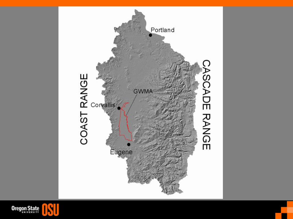
Project GoalProject Goal

To develop a three-dimensional groundwater flow model to be used as a tool by local policy makers, water quality educators, and scientists to help make

management decisions.

Qalc = Upper Sedimentary Unit

Qff2 Qalf = Willamette Silt Unit

Qg1 Qg2 = Middle Sedimentary Unit Qbf = Lower Sedimentary Unit

*Bedrock units not included in model

Geologic and Geologic and Hydrogeologic UnitsHydrogeologic Units

5 miles

N

[Modified from O’Connor et al., 2001]

B B’

Qalc, Upper Sedimentary Unit

[Modified from O’Connor et al., 2001]

Qff2, Willamette Silt Unit

Qg2, part of the Middle Sedimentary Unit

[Modified from O’Connor et al., 2001]

Qg2, part of the Middle Sedimentary Unit

[Modified from O’Connor et al., 2001]

Field WorkField Work• Water level

measurements- 6 sets of quarterly

measurements from network of 42 wells, 14 from Oregon Water Resources Department, 1 from Eugene Water and Electric Board

- Long-term water level

data from 3 locationsLong Tom River

McKenzie River

Muddy Creek

Calapooia River

South Santiam River

Mary’s River

5 miles

N

[Modified from O’Connor et al., 2001]

Field WorkField WorkAquifer Tests

Pump Tests (N = 3) - ranges of K from 1.0 x 102 - 1.7 x 103 ft/day;

3.5 x 10-4 - 6.0 x 10-3 m/s - Neuman curve-fitting method

Slug Tests (N = 17) - ranges of K from 4.0 x 10-2 - 4.3 x 102 ft/day;

1.4 x 10-7 - 1.5 x 10-3 m/s - Bouwer-Rice’s method

Construction of cross-sections and stratigraphic columns

Field WorkField Work

• Groundwater age and chemistry sampling

• Results indicate ages from 13 to >57 years [Conlon et al., 2005 and this study]

• Groundwater sampled where

Qff2 exists greater in age than groundwater sampled where no Qff2 exists

[Modified from O’Connor et al., 2001]

MODFLOW w/GMS ModelMODFLOW w/GMS Model

MODFLOW w/GMS ModelMODFLOW w/GMS Model

Upper Sedimentary Unit

Middle Sedimentary Unit

Lower Sedimentary Unit

Willamette River

x30 vertical exaggeration

MODFLOW w/GMS ModelMODFLOW w/GMS Model

South Santiam River

Calapooia River

Muddy Creek

McKenzie River

Willamette River

Long Tom River

Mary’s River

NO FLOW Boundary

Generalized Head Boundary

Generalized Head Boundary

Generalized Head Boundary

5 miles

BOUNDARY CONDITIONS

MODFLOW w/GMS ModelMODFLOW w/GMS Model

• Model input

- River stage, discharge, and conductance

- Recharge

- Potential evapotranspiration

w

tRiver Bed

River

River surface

River bottom

MODFLOW w/GMS ModelMODFLOW w/GMS Model

• Steady-state model developed

• Used “average”- water level- river stage and flow - potential evapotranspiration (45 in/year)- precipitation (28 in/year)

data from June 2004 – July 2005

• Used hydraulic conductivity estimates from local pump/slug tests and specific capacity data to simulate spatial heterogeneity

Willamette Silt

5 miles

Kh = 0.1 ft/dayKh/Kv = 100

Upper Sedimentary Unit

Kh = 550 ft/dayKh/Kv= 50

5 miles

Kh = 10 - 500 ft/day (x12)Kh/Kv = 50

Middle Sedimentary Unit

5 miles

Kh = 7 - 105 ft/day (x12)Kh/Kv = 50

Lower Sedimentary Unit

5 miles

MODFLOW w/GMS ModelMODFLOW w/GMS Model

• Model Calibration

- Gain and loss of river stream reaches

- Total Flow in vs. Total Flow out (~0.05% discrepancy)

Compared simulated vs. observed:

Water levels in well network

Groundwater ages using MODPATH

Initial MODPATH results

5 miles

- Modeled ≈ Measured

Observation wells

5 miles

Mean Error: 0.02 ft Mean Abs. Error: 6.9 ftRoot Mean Sq. Error: 8.4 ft

MODFLOW w/GMS ModelMODFLOW w/GMS Model

200

250

300

350

400

450

200 250 300 350 400 450

Computed vs. Observed ValuesHead

Com

pute

d

Observed

20 ft. contours

Simulated Head Contour Map

5 miles

Preliminary Results/Conclusions Preliminary Results/Conclusions 1/21/2

• MODFLOW-MODPATH along with groundwater age and chemistry data useful in determining fate of nitrate (Willamette Silt vs. no Willamette Silt)

• Geology in the SWV plays a large role in determining groundwater flow and nitrate transport (Iverson 2002, Kite-Powell 2003, Vick 2004, Arighi 2004, Oregon DEQ’s work, and this study)

• Time-scale of problem 10’s of years

• The model will be made available to public

Preliminary Results/Conclusions Preliminary Results/Conclusions 2/22/2

• The model will be used for public presentations as a tool to help illustrate and describe groundwater flow

• The model will be able to help answer questions addressed by the GWMA Committee

- Where is the nitrate coming from?

- How long?

- How can we reduce current nitrate levels?

• Future work with model includes using projected land-uses in the Southern Willamette Valley to determine effects on groundwater flow, nitrate transport, and groundwater management

Thanks!Thanks!

• To the Environmental Protection Agency for funding (Regional Geographic Initiative 2004 grant # X5-970838-01)

• To the many people and agencies who have contributed time and information as this project developed