Ground-Water Hydraulics - USGS hydraulics by s. w. lohman geological survey professional paper 708...
78
Ground-Water Hydraulics GEOLOGICAL SURVEY PROFESSIONAL PAPER 708
Transcript of Ground-Water Hydraulics - USGS hydraulics by s. w. lohman geological survey professional paper 708...
Ground-Water Hydraulics
GEOLOGICAL SURVEY PROFESSIONAL PAPER 708
Ground-Water HydraulicsBy S. W. LOHMAN
GEOLOGICAL SURVEY PROFESSIONAL PAPER 708
UNITED STATES GOVERNMENT PRINTING OFFICE, WASHINGTON : 1972
UNITED STATES DEPARTMENT OF THE INTERIOR
ROGERS C. B. MORTON, Secretary
GEOLOGICAL SURVEY
V. E. McKelvey, Director
First printing 1972
Second printing 1975
For sale by the Superintendent of Documents, U.S. Government Printing OfficeWashington, D.C. 20402 - Price $4.15 (paper cover)
Stock Number 024-001-01194
CONTENTS
Symbols and dimensions._--... ..-.-.....____._._.Introduction----__.-----__----_-----_---------_.______Divisions of subsurface water in unconfined aquifers______
Saturated zone.-_---_-_-_---___---_-_--___________Water table............_..._..............Capillary fringe_.-_---------_----.-.--._.....
Unsaturated zone--.-------.----------------.......Capillarity..........---.-.--..----..----------......__Hydrologic properties of water-bearing materials._-..___.__
Porosity ..........................................Primary.-___._._._-_-.___--------------_-_.__Secondary --------__----_-.---------.._-..
Conditions controlling porosity of granular materials. . .Arrangement of grains (assumed spherical and of
equal size)---_-.--._..-_.-.-.--_.----._...._Shape of grains---------_--_---------_---_____-Degree of assortment......-_-----...._........_
Void ratio_..------------_.--.-....--_._...__..Permeabili ty -.-----------____---------_-_-________Intrinsic permeability---.------_-----.--...._......Hydraulic conductivity.__......_..____Transmissivity _ . ..._._.__...-_--_----._...___._
Water yielding and retaining capacity of unconfined aquifers.. Specific yield..------------.--------------..-._.,__Specific retention.__-_-_-__---,--___--________.___Moisture equivalent-_______________________________
Artesian wells confined aquifers____-------_______.____Flowing wells unconfined aquifers_. ...................Confined aquifers ...................^..................
Potentiometric surface_-------_---_--__-_-_______-Storage properties.--_--_--___--_-----_---_-__..____
Storage coefficient__.......--__---._..__.-..-.Components _ _____-_-..---.----...._.....
Land subsidence._-.-_.__-.------.-_..._.._....Elastic confined aquifers.-___-_--___________Nonelastic confined aquifers and oil-bearing
strata_-__-_----_-.-----_______________Movement of ground water steady-state flow___.._._.__
Darcy's law.__------_--_-_-____-__________________Velocity --___----_----______-..-__......__._......
Aquifer tests by well methods point sink or point source... Steady radial flow without vertical movement.________
Example..___-----__-_______-_________________Partial differential equations for radial flow.__________Nonsteady radial flow without vertical movement......
Constant discharge.-_-.._..........____..__..._Example. ---__--_--___-__-._._____________Straight-line solutions._____________________
Transmissivity__ ____________________Storage coefficient___.----.___...._.._
Example________________________Precautions. __________________________
VI 1 1 1122233444
444445666666778888999
9101010111112131515191919212222
Page Aquifer tests by well methods Continued
Nonsteady radial flow without vertical movement Continued
Constant drawdown ______._-______----______ 23Straight-line solutions---... ..__ 23
Example___._____..._..___ 25Instantaneous discharge or recharge______________ 27
"Slug" method..._-__._______--__----_-_ 27Example. _-_.----....---_---.-_._-_.._ 29
Bailer method-___._.---------------------- 29Leaky confined aquifers with vertical movement-..____ 30
Constant discharge.........._._.._-__.---___._. 30Steady flow.____------_----.__.-.--__.__ 30Nonsteady flow..____________------_---____ 30
Hantush-Jacob method._-_---_-_-----._ 30Example. --_----_._-------------.- 31
Hantusb modified method.-------------- 32Example_....._....._____. 32
Constant drawdown.-.__..........-_.-_-.-_.._. 34Unconfined aquifers with vertical movement_____ 34
Example for anisotropic aquifer....-._--._---_._. 36Example for delayed yield from storage.. ..... 38
Aquifer tests by channel methods line sink or line source(nonsteady flow, no recharge).. ----_---.-.-----.---._ 40
Constant discharge_..---_._..._.._-----.-_-_-__._ 40Constant drawdown.----------------.---------.---- 41
Aquifer tests by areal methods____--._.._..--------..._ 43Numerical analysis...------------_.-.-------------- 43
Example.......--------.----_----------------- 44Flow-net analysis._---.-..--_-..-_.--.---_-----.--- 45
Example . _-_.-------_-------------.-----.-_- 45Closed-contour method--_.---------------_-----_-.- 46Unconfined wedge-shaped aquifer bounded by two
streams.-.--_-------------------__-------------- 49Methods of estimating transmissivity___._---_----__.___ 52
Specific capacity of wells---.---.-------------------- 52Logs of wells and test holes.____--..----------.---.- 53
Methods of estimating storage coefficient__--_--_--___-_- 53Methods of estimating specific yield..-.-.__--------__-_._ 53Drawdown interference from discharging wells.._----__--__ 55Relation of storage coefficient to spread of cone of depression. 56Aquifer boundaries and theory of images.__-___--_--__-___ 57
"Impermeable" barrier._____________-_-_--_------._ 57Line source at constant head perennial stream ____ 58Application of image theory.________.._---___---_. 59
"Safe yield".____________________..._.................. 61The source of water derived from wells-_-__--_---------_- 62
Examples of aquifers and their development ________ 64Valley of large perennial stream in humid region. _ _ 64Valley of ephemeral stream in semiarid region _ _ _ _ . 64Closed desert basin________________.__..___.___. 65Southern High Plains of Texas and New Mexico 65Grand Junction artesian basin, Colorado.______--- 66
References cited-____._-------------___---------------- 67
III
IV CONTENTS
ILLUSTRATIONS
[Plates are in pocket]
PLATE 1. Logarithmic plot of a versus (?(«).2. Type curves for H/H0 versus Tt/rcz for five values of a;3. Two families of type curves for nonsteady radial flow in an infinite leaky artesian aquifer.4. Family of type curves for 1/u versus H(u, /3), for various values of j8.5. Logarithmic plot of a versus G(a, rw/B).6. Curves showing nondimensional response to pumping a fully penetrating well in an unconfined aquifer.7. Curves showing nondimensional response to pumping a well penetrating the bottom three-tenths, of the thickness of an unconfine.d
aquifer.8. Delayed-yield type curves.9. Logarithmic plot of SW(w) versus l/up .
Page
FIGURE 1. Diagram showing divisions of subsurface water in unconfined aquifers-__-_-_---_-_-_-__--.__-_.___..___.---_--... 2 2-5. Sketches showing
2. Water in the unsaturated zone__----_-_---___-__-_________-.______-_____._____._.__._.____________._ 23. Capillary rise of water in a tube___---------------_----_-_-_-_---_-_-__-_-_--_--_.-._.-._.._______. 34. Rise of water in capillary tubes of different diameters__._.____.___-__-_-_._.__._____..__.__.__.._.____ 35. Sections of four contiguous spheres of equal size____._.___-._-__-__--_-_--__-__--.__.__-___.____-._._. 4
6. Graph showing relation between moisture equivalent and specific retention___.__-__-___.___._._.______._-_____. 77. Diagrammatic section showing approximate flow pattern in uniformly permeable material which receives recharge in
interstream areas and from which water discharges into streams__._______.--___-__---__-_-__________________ 78. Diagrammatic sections of discharging wells in a confined aquifer and an unconfined aquifer._______.___..__..___._.._ 89. Sketch showing hypothetical example of steady flow________________________________________________________ 10
10. Half the cross section of the cone of depression around a discharging well in an unconfined aquifer -______._.____.^______ 1111. Semilogarithmic plot of corrected drawdowns versus radial distance for aquifer test near Wichita, Kans ___________^_____ 1312. Sketch of cylindrical sections of a confined aquifer_____________________________________________________________ 1413. Sketch to illustrate partial differential equation for steady radial flow.--_-__-_-_-_--_____-__-_-_-____-_______-.__ 1414. Logarithmic graph of W(u) versus u......................................................................... 1715. Sketch showing relation of W(u) and u to s and r*/t, and displacements of graph scales by amounts of constants shown. _ _ _ _ 1816. Logarithmic plot of s versus r*/t from table 6__-_-___-_-__.-_-____-_-___----__-__-___-_______________--_---__ 20
17-19. Semilogarithmic plot of 17. sw/Q versus t/rw2..........,....^.............. _..._...___..._.__.........._._...._.._....-...... 2518. Recovery (sw) versus t................................................_._......._..._..._.__........ 2619. Data from "slug" test on well at Dawsonville, Ga__.___._._._._. .....................^..^. ___________ 28
20. Logarithmic plot of s versus t for observation well 23S/25E-17Q2 at Pixley, Calif _.__.._._____..__________ 3321. Sketch showing relation of 2 to b of pumped and observation wells on plates 6 and 7............................... 35
22-25. Logarithmic plot of 22. s versus t for observation well B2-66-7dda2, near lone, Colo____._.-___.___________________._._-__--__ 3723. s versus t for observation well 139, near Fairborn, Ohio._____-._.-..__.___._.-._._.-___...._._.__-_._-_- 3924. D(u) q versus w2 for channel method constant discharge____-__-_____-___________-_---_______---_---_- 4125. D(u)h versus uz for channel method constant drawdown...._._.____._..._-.___.____-___-___-.-_.--_---__ 42
26. Sketch showing array of nodes used in finite-difference analysis___!_____ _____.__-.-_-_.--_-_-.--__-.-._-----__. 4427. Plot of 2ft versus Aft0/AJ for winter of 1965-66, when W=0..................................................... 4628. Plot of 2A versus AAo/Af for spring-of 1966.._..........._..,.. ----------._._...._...................... __ 4729. Sketch showing idealized square of flow net_..__------------ ---------- ----- -. ------ 4730. Map of Baltimore industrial area, Maryland, showing potentiometric surface in 1945 and generalized flow lines in the
Patuxent Formation ...............................................^................................... 4831. Sketch map of a surface drainage pattern, showing location of observation wells that penetrate an unconfined aquifer. _____ 4932. Example hydrograph from well A of figure 31, showing observed and projected water-level altitudes__________.--.__ 5033. Graph of S/SQ versus t taken from hydrograph of well A (see fig. 32), showing computation of T/S..^................ 5034. Graph of s/s0 versus Tt/i*S for 00 = 75°; 6/6a =0.20............................................................ 5135. Family of Semilogarithmic curves showing the drawdown produced at various distances from a well discharging at stated
rates for 365 days from a confined aquifer for which T = 20 ftzday-1 and S= 5X 10~6 _____--___-_-_----_-_-----_ 5436. Family of Semilogarithmic curves showing the drawdown produced after various times at a distance of 1,000 ft from a
well discharging at stated rates from a confined aquifer for which T = 20 ft2day-1 and S= 5X 10~5_______----_-_-- 5537. Idealized section views of a discharging well in an aquifer bounded by an "impermeable" barrier and of the equivalent
hydraulic system in an infinite aquifer_______________________________________________-_---_-__-_-------- 5638. Generalized flow net in the vicinity of discharging real and image wells near an "impermeable" boundary __-__-__- 5739. Effect of "impermeable" barrier on Semilogarithmic plot of s versus i/r2 .._________-_-__-_-_-_______----_------- 5840. Idealized section views of a discharging well in an aquifer bounded by a perennial stream and of the equivalent hydraulic
system in an infinite aquifer___.._.._..._.._.._..____.____.__....______..____-_-_----_--__--------_--- 59
CONTENTS V
Page41. Generalized flow net in the vicinity of a discharging well dependent upon induced infiltration from a nearby stream___ __ 6042. Effect of recharging stream on semilogarithmic plot of s versus t/r*. __.._..__._______._._._.._...__._....__._._.____ 61
43-47. Diagrammatic sections showing development of ground water from 43. Valley of large perennial stream in humid region...._...._-._.__..._..____._._.__...._._..__._.___.___. 6444. Valley of ephemeral stream in semiarid region.__...._.._....._...__....___..._.___.___._..._...._._.... 6445. Bolson deposits in closed desert basin________-..--._.._-_---__.-.-.-_-.__._._..._..___..._..._....._ 6546. Southern High Plains of Texas and New Mexico.-__-_-_-_--_----_-_--_-_----___-_____---_-_-_-_-__-_._ 6647. Grand Junction artesian basin, Colorado__-_-__--_--_--__-__-__--____-_________-_-------_-_-___--___ 66
TABLES
Page TABLE 1. Capillary rise in samples having virtually the same porosity, 41 percent, after 72 days____-_..__-_-_---_-.._._.._ 3
2. Relation of units of hydraulic conductivity, permeability, and trarismissivity_.__.______..__________.._._.___.__._. 53. Land subsidence in California oil and water fields--------_--_----_--_-----_____---_____________-________________ 104. Data for pumping test near Wichita, Kans_._________________________________________________________________ 125. Values of W(u) for values of u between 10~15 and 9.9----------_--------_-_-_-_----____-_-_-_-_____-___-________ 166. Drawdown of water level in observation wells N-l, N-2, and N-3 at distance r from well being pumped at constant rate
of 96,000 ft8 day-1............--.--................-....________________________________________________ 197. Values of G(a) for values of a between 10"* and 1015_____--_____-_-________.________.___________________________ 248. Field data for flow test on Artesia Heights well near Grand Junction, Colo., September 22, 1948-___-_-__--___-_-____ 249. Field data for recovery test on Artesia Heights well near Grand Junction, Colo., September 22, 1948._-,____--_-______ 26
10. Recovery of water level in well near Dawsonville, Ga., after instantaneous withdrawal of weighted float_.__-.-______ 2911. Postulated water-level drawdowns in three observation wells during a hypothetical test of ah infinite leaky confined aquifer. 31
12-14. Drawdown of water levels in 12. Observation well 23S/25E-17Q2, 1,400 ft from a well pumping at constant rate of 750 gpm, at Pixley, Calif.,
March 13, 1963.. ______ _ _____ _ _ ____ _ _ _ __________________________________________________ 3213. Observation well B2-66-7dda2, 63.0 ft from a well pumping at average rate of 1,170 gpm, near lone, Coio.,
August 15-18, 1967.________________________________________________________....................... 3814. Observation well 139, 73 ft from a well pumping at constant rate of 1,080 gpm, near Fairborn, Ohio, October
19-21, 1954______.._._.____._............I ______________________________________________________ 3815. Values of D(u)<,, u, and u2 for channel method constant discharge.------------_-_______-_____________._._____-__ 4116. Values of D(u\ u, and u? for channel method constant drawdown___________________________________________ 4317. Average values of hydraulic conductivity of alluvial materials in the Arkansas River valley, Colorado__-.____-.-____ 5318. Computations of drawdowns produced at various distances from a well discharging at stated rates for 365 days from a
confined aquifer for which T = 20 ft2 day-1 and S=5X10⁻⁶...-.________________.._._____________.._..._____ 5419. Computations of drawdowns produced after various times at a distance of 1,000 ft from a well discharging at stated rates
from a confined aquifer for which T = 20 ft2 day-1 and S = 5X10"5-----__..__..________.__________ 55
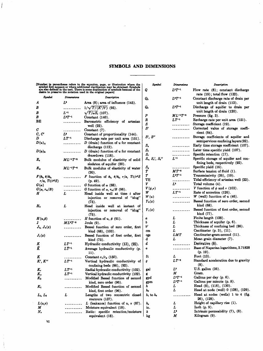
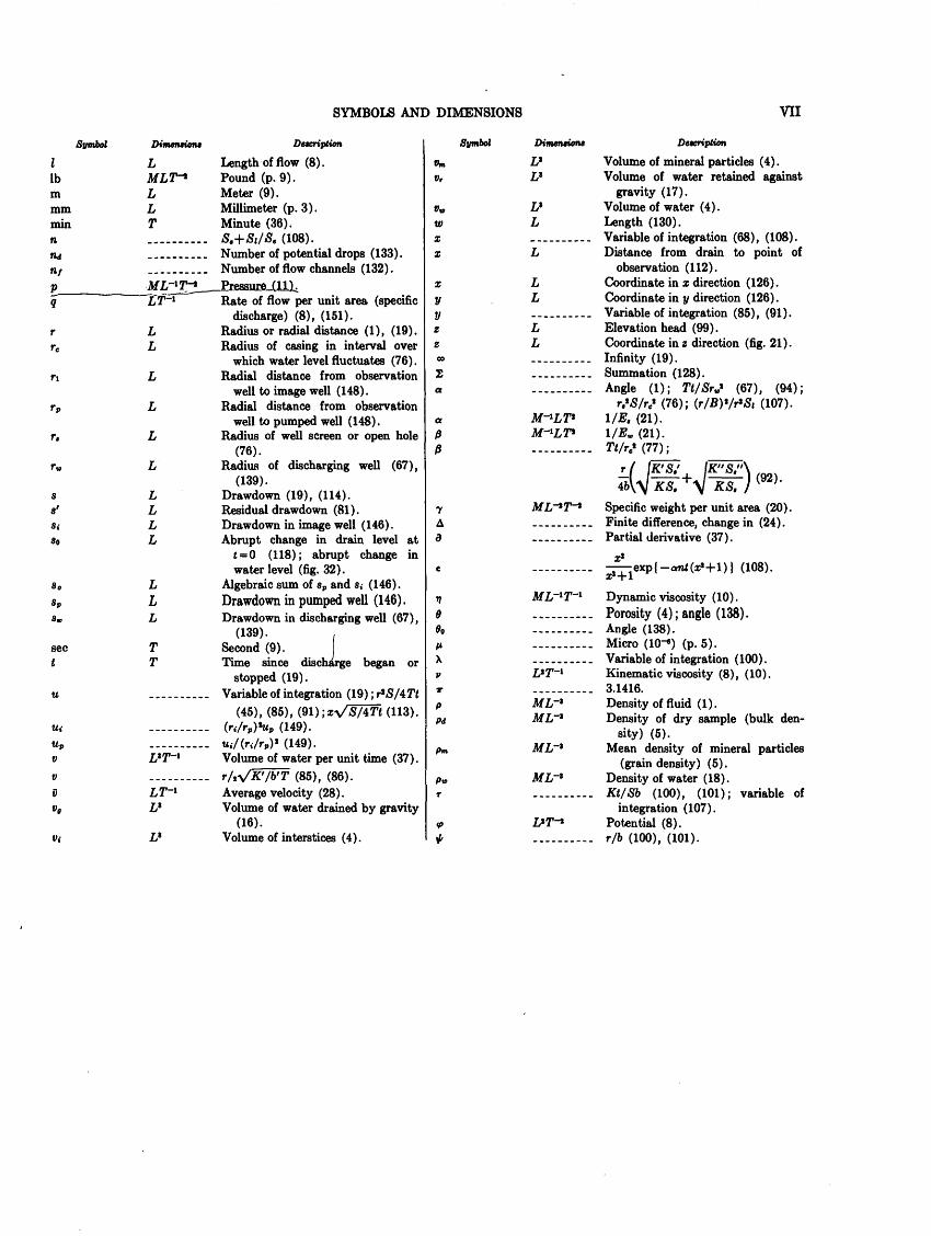
[Number in parentheses refers to the equation, page, or illustration where the symbol first appears or where additional clarification may be obtained. Symbols are also defined in the text. There is some duplication of symbols because of the desire to preserve the notation used in the original papers]
Symbol
A B B B BE
CC,C'DD(u),
E.
DimmtiontL*
L*
r/a, Tt/r*S)
H
JJo, Jt(x)
K
K K', K"
Kr K,
Li, Li
L(u,v) M
VI
Detcription
Area (8) ; area of influence (145) . l/VT/(K'/V) (95).
(107).
Tt/r*S
t after "slug"
Constant (140).Barometric efficiency of artesian
well (22). Constant (7).Constant of proportionality (144). Discharge rate per unit area (151). D (drain) function of u for constant
discharge (112). D (drain) function of u for constant
drawdown (118). Bulk modulus of elasticity of solid
skeleton of aquifer (20) . Bulk modulus of elasticity of water
(20). F function of 80, O/Oo, r/a,
(p. 49).G function of a (68). G function of a, rv/B (96). Head inside well at time
injection or removal of(75).
Head inside well at instant ofinjection or removal of "slug"(75).
H function of u, ft (91). Joule (9). Bessel function of zero order, first
kind (68), (100). Bessel function of first order, first
kind (75).Hydraulic conductivity (13), (92). Average hydraulic conductivity (p.
H).Constant n/rp (150). Vertical hydraulic conductivity of
confining beds (86), (92). Radial hydraulic conductivity (102) . Vertical hydraulic conductivity (102). Modified Bessel function of second
kind, zero order (96) . Modified Bessel function of second
kind, first order (96). Lengths of two concentric closed
contours (137).L (leakance) function of u, v (87). Moisture equivalent (18). Ratio: specific retention/moisture
equivalent (18).
Symbol
P RS S'
S', S"
S. StSr
S., S.', S."
T TTE V
W W(u)
abVcmcgsdde
ft Q
galggpdgpmhJ*>hi to
he in. k kg
Dimmnont Description
HT-i Flow rate (8); constant discharge rate (19); total flow (132).
L*T~l Constant discharge rate of drain per unit length of drain (112).
£171-1 Discharge of aquifer to drain per unit length of drain (120).
ML-iT-t Pressure (fig. 3).LT~l Recharge rate per unit area (151)..___..._._ Storage coefficient (19).----.---.- Corrected value of storage coeffi
cient (64)._-_-_--__- Storage coefficients of aquifer and
semipervious confining layers (92)._-.-_---.. Early time storage coefficient (107).____._--._ Later time specific yield (107).___-..--_- Specific retention (17).L~} Specific storage of aquifer and con
fining beds, respectively (92).--_-.--.-- Specific yield (16).M T~* Surface tension of fluid (1).£471-1 Transmissivity (26), (19)._-___.-__- Tidal efficiency of artesian well (22).L» Total volume (4).______ V function of ^ and T (103).LT~l Rate of accretion (126)..... _... W (well) function of u (46).---__---_- Bessel function of zero order, second
kind (68). _.-__---.- Bessel function of first order, second
kind (77).L Finite length (128). L Thickness of aquifer (p. 6). L Thickness of confining bed (86). L Centimeter (p. 3), (11). LMT Centimeter-gram-second (11). L Mean grain diameter (7). _____ Derivative (8)._-_-_---_- Base of Naperian logarithms, 2.71828
(p. 19).L Foot (13). LT~* Standard acceleration due to gravity
(8).U U.S. gallon (36). M Gram. LT-1 Gallons per day (p. 6). L*T~l Gallons per minute (p. 8). L Head (8), (116), (130). L Head at node (well) 0 (128), (129). _____. Head at nodes (wells) 1 to 4 (fig.
26), (128).L Height of capillary rise (1). L Inch (p. 9). L* Intrinsic permeability (7), (8). M Kilogram (9).
SYMBOLS AND DIMENSIONS VII
Symbol
I
lbmmmminnridnf
-
Dimmriant
L
sec t
L L T
LT~l
L L
L L L
T T
Detention
Length of flow (8).Pound (p. 9).Meter (9).Millimeter (p. 3).Minute (36).S.+St/S, (108).Number of potential drops (133) .Number of flow channels (132) .
L*
Rate of flow per unit area (specificdischarge) (8), (151).
Radius or radial distance (1), (19). Radius of casing in interval over
which water level fluctuates (76) . Radial distance from observation
well to image well (148). Radial distance from observation
well to pumped well (148). Radius of well screen or open hole
(76). Radius of discharging well (67),
(139).Drawdown (19), (114). Residual drawdown (81). Drawdown in image well (146). Abrupt change in drain level at
t=0 (118); abrupt change inwater level (fig. 32).
Algebraic sum of sp and s< (146). Drawdown in pumped well (146).Drawdown in discharging well (67),
(139). Second (9). Time since discharge began
stopped (19). Variable of integration ( 19) ; r*»S/4 Tt
(45), (85), (91);x\/is74T« (113). (r,-/rp )*Mp (149). tt,/(r</rp)» (149). Volume of water per unit time (37).
(85), (86).Average velocity (28). Volume of water drained by gravity
(16). Volume of interstices (4).
Symbol Dimmtiona Description
Um L* Volume of mineral particles (4).vr L' Volume of water retained against
gravity (17).vw L* Volume of water (4).w L Length (130).x ..... _.. Variable of integration (68), (108).x L Distance from drain to point of
observation (112).x L Coordinate in x direction (126).y L Coordinate in y direction (126).y ______ Variable of integration (85), (91).z L Elevation head (99).z L Coordinate in z direction (fig. 21).» ....._.. Infinity (19).2 _____. Summation (128).a .......... Angle (1); Tt/SrJ (67), (94);
r.*S/rc» (76); (r/B)*/r*St (107). a M-*LT* l/E. (21). /3 M-iLT* l/E, (21). ft .......... 2Vr.«(77)£_ ___
rjf [KM {&8?\ 4&VV K8. +\ KS. ) (92) '
y ML~*T~* Specific weight per unit area (20).A -.--.-..-. Finite difference, change in (24).d .......... Partial derivative (37).
(108).
j> ML~l T~l Dynamic viscosity (10). e .......... Porosity (4); angle (138).0o .......... Angle (138).M .......... Micro (10-«) (p. 5).X .---..-.-. Variable of integration (100).v L*T~l Kinematic viscosity (8), (10).r .......... 3.1416.p ML~* Density of fluid (1).Pd ML~l Density of dry sample (bulk den
sity) (5).Pm ML~* Mean density of mineral particles
(grain density) (5).p«, ML~* Density of water (18).T .......... Kt/Sb (100), (101); variable of
integration (107).<? L*T~* Potential (8).* .......... r/6 (100), (101).
GROUND-WATER HYDRAULICS
By S. W. LOHMAN
INTRODUCTION
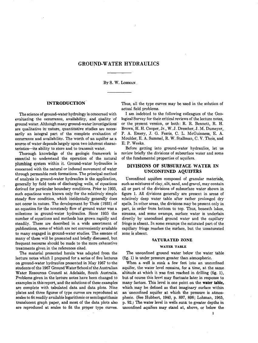
The science of ground-water hydrology is concerned with evaluating the occurrence, availability, and quality of ground water. Although many ground-water investigations are qualitative in nature, quantitative studies are neces sarily an integral part of the complete evaluation of occurrence and availability. The worth of an aquifer as a source-of water depends largely upon two iriherent charac teristics its ability to store and to transmit water.
Thorough knowledge of the geologic framework is essential to understand the operation of the natural plumbing system within it. Ground-water hydraulics is concerned with the natural or induced movement of water through permeable rock formations. The principal method of analysis in ground-water hydraulics is the application, generally by field tests of discharging wells, of equations derived for particular boundary conditions. Prior to 1935, such equations were known only for the relatively simple steady flow condition, which incidentally generally does not occur in nature. The development by Theis (1935), of an equation for the nonsteady flow of ground water was a milestone in ground-water hydraulics. Since 1935 the number of equations and methods has grown rapidly and steadily. These are described in a wide assortment of publications, some of which are not conveniently available to many engaged in ground-water studies. The essence of many of these will be presented and briefly discussed, but frequent recourse should be made to the more exhaustive treatments given in the references cited.
The material presented herein Was adapted from the lecture notes which I prepared for a series of five lectures on ground-water hydraulics presented in May 1967 to vthe students of the 1967 Ground Water School of the Australian Water Resources Council at Adelaide, South Australia;. Problems given in the lecture notes have been changed to examples in this report, and the solutions of these examples are complete with tabulated data and data plots. Nine plates and three figures of type curves are reproduced at scales to fit readily available logarithmic or semilogarithmic translucent graph paper, and most of the data plots also are reproduced at scales to fit the proper type curves.
Thus, all the type curves may be used in the solution of actual field, problems.
I am indebted to the following colleagues of the Geo logical Survey for their critical reviews of the lecture notes, or the present version, or both: R. R. Bennett, R. H. Brown, H. H. Cooper, Jr., W.. J. Drescher, J, M. Dumeyer,. P. A. Emery, J. G. Ferris, C. L. McGuinness, E. A. Moulder, E. A. Sammel, R. W. Stallman, C. V. Theis, and E. P. Weeks.
Before getting into ground-water hydraulics, let us review briefly the divisions of subsurface water and some of the fundamental properties of aquifers.
DIVISIONS OF SUBSURFACE WATER IN UNCONFINED AQUIFERS
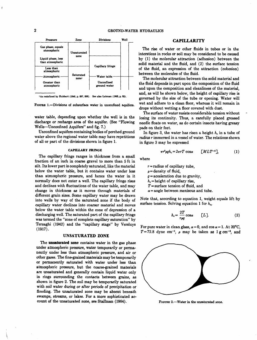
Unconfined aquifers composed of granular materials, such as mixtures of clay, silt, sand, and gravel, may contain all or part of the divisions of subsurface water shown in figure 1. All divisions generally are present in areas of relatively deep water table after rather prolonged dry spells. In other areas, the divisions may be present only in part, in order from bottom to top. Thus, beneath lakes, streams, and some swamps, surface water is underlain directly by unconfiried ground water and the capillary fringe is absent. In some swamps the saturated part of the capillary fringe reaches the surface, but the unsaturated zone is absent.
SATURATED ZONE
WATER TABLE
The unconfined ground water below the water table (fig. 1) is uncjer pressure greater than atmospheric.
When a >well is sunk a few feet into an unconfined aquifer, the water level remains, for a time, at the same altitude at which it was first reached in drilling (fig. 1), but of course this level may fluctuate later in response to many factors. This level is, one point on the water table, which.may.be defined as that imaginary surface within an unconfined aquifer at which the pressure is atmos pheric. (See Hubbert, 1940, p. 897, 898; Lohman, 1965, p. 92.; The water level in wells sunk to greater depths in unconfined aquifers may stand at, above, or below the
l
GROUND-WATER HYDRAULICS
Pressure Zone Divisions Well
Gas phase, equals atmospheric
Liquid phase, less than atmospheric
Less than atmospheric
Greater than atmospheric
Unsaturated
Saturatedzone'
Water table
Unconfirmed ground water
i As redefined by Hubbert (1940, p. 897, 898). See also Lohman (1965, p. 92).
FIGUBE 1. Divisions of subsurface water in unconfined aquifers.
water table, depending upon whether the well is in the discharge or recharge area of the aquifer. (See "Flowing Wells Unconfined Aquifers" and fig. 7.)
Unconfined aquifers containing bodies of perched ground water above the regional water table may have repetitions of all or part of the divisions shown in figure 1.
CAPILLARY FRINGE
The capillary fringe ranges in thickness from a small fraction of an inch in coarse gravel to more than 5 ft in silt. Its lower part is completely saturated, like the material below the water table, but it contains water under less than atmospheric pressure, and hence the water in it normally does not enter a well. The capillary fringe rises and declines with fluctuations of the water table, and may change in thickness as it moves through materials of different grain sizes. Some capillary water may be drawn into wells by way of the saturated zone if the body of capillary water declines into coarser material and moves below the water table within the cone of depression of a discharging well. The saturated part of the capillary fringe was termed the "zone of complete capillary saturation" by Terzaghi (1942) and the "capillary stage" by Versluys (1917).
UNSATURATED ZONE
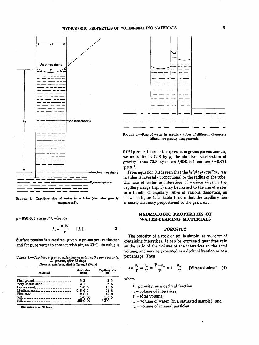
The nnsaturated zone contains water in the gas phase under atmospheric pressure, water temporarily or perma nently under less than atmospheric pressure, and air or other gases. The fine-grained materials maybe temporarily or permanently saturated with water under less than atmospheric pressure, but the coarse-grained materials are unsaturated and generally contain liquid water only in rings surrounding the contacts between grains, as shown in figure 2. The soil may be temporarily saturated with soil water during or after periods of precipitation or flooding. The unsaturated zone may be absent beneath swamps, streams, or lakes. For a more sophisticated ac count of the unsaturated zone, see StaUman (1964).
CAPILLARITY
The rise of water or other fluids in tubes or in the interstices in rocks or soil may be considered to be caused by (1) the molecular attraction (adhesion) between the solid material and the fluid, and (2) the surface tension of the fluid, an expression of the attraction (cohesion) between the molecules of the fluid.
The molecular attraction between the solid material and the fluid depends in part upon the composition of the fluid and upon the composition and cleanliness of the material, and, as will be shown below, the height of capillary rise is governed by the size of the tube or opening. Water will wet and adhere to a clean floor, whereas it will remain in drops without wetting a floor covered with dust.
The surface of water resists considerable tension without losing its continuity. Thus, a carefully placed greased needle floats on water, as do certain insects having greasy pads on their feet.
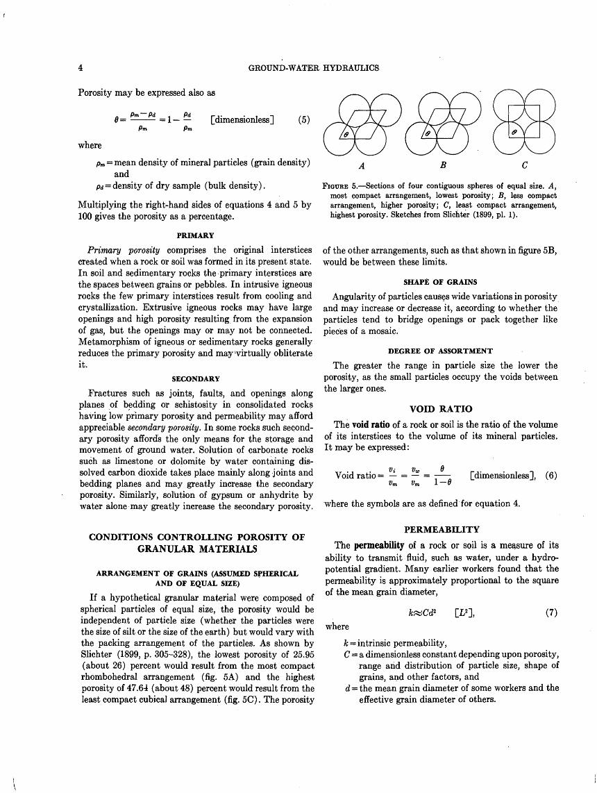
In figure 3, the water has risen a height hc in a tube of radius r immersed in a vessel of water. The relations shown in figure 3 may be expressed
(1)
where
r=radius of capillary tube,p = density of fluid,g = acceleration due to gravity,hc = height of capillary rise,r=surf ace tension of fluid, anda = angle between meniscus and tube.
Note that, according to equation 1, weight equals lift by surface tension. Solving equation 1 for he>
2The = cosa TLl.
rpg(2)
For pure water in clean glass, a = 0, and cos a = 1. At 20°C, 7=72.8 dyne cm"1, p may be taken as 1 g cm~3, and
FIGURE 2. Water in the unsaturated zone.
HYDROLOGIC PROPERTIES OF WATER-BEARING MATERIALS
P= atmospheric
X
XX
P<atmospheric
-P= atmospheric
-P>atmospheric
FIGURE 3. Capillary rise of water in a tube (diameter greatly exaggerated).
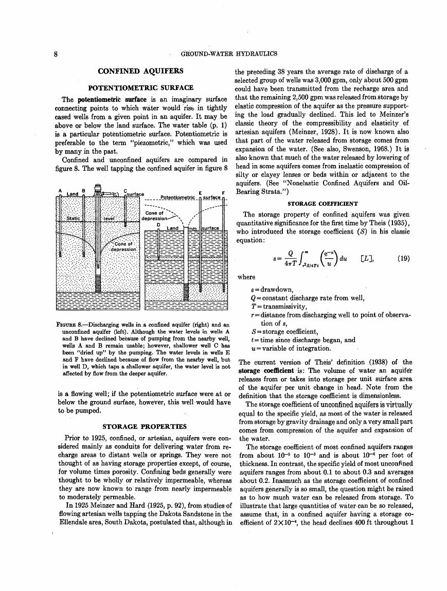
FIGURE 4. Rise of water in capillary tubes of different diameters (diameters greatly exaggerated).
0.074 g cm"1 . In order to express it in grams per centimeter, we must divide 72.8 by g, the standard acceleration of gravity; thus 72.8 dyne cm-l/980.665 cm sec"2 = 0.074 g cm~l .
From equation 3 it is seen that the height of capillary rise in tubes is inversely proportional to the radius of the tube. The rise of water in interstices of various sizes in the capillary fringe (fig. 1) may be likened to the rise of water in a bundle of capillary tubes of various diameters, as shown in figure 4. In table 1, note that the capillary rise is nearly inversely proportional to the grain size.
g = 980.665 cm sec~2, whence
= ra. (3)
Surface tension is sometimes given in grams per centimeter and for pure water in contact with air, at 20°C, its value is
TABLE 1. Capillary rise in samples having virtually the same porosity, 41 percent, after 72 days
[From A. Atterberg, cited in Terzaghi (1942)]
Material
Fine gravel __ __.....__.___.Very coarse sand ._____-.Coarse sand. ..-.----...._._Medium sand __ ----------Fine sand. -----------------Silt .....................Silt
Grain sice (mm)
..... 5-2
..... 2-1
..... 1-0.5----- 0.5-0.2..... .2-0.1..... .1-0.05..... .05-0.02
Capillary rise (cm)
2.56.5
13.524.642.8
105.51 200
HYDROLOGIC PROPERTIES OF WATER-BEARING MATERIALS
POROSITY
The porosity of a rock or soil is simply its property of containing interstices. It can be expressed quantitatively as the ratio of the volume of the interstices to the total volume, and may be expressed as a decimal fraction or as a percentage. Thus
n Vi Vw V Vm Vm -in ,A\0= - = = y- =1- [dimensionless] (4)
where
* Still rifling after 72 days.
9 = porosity, as a decimal fraction,Vi= volume of interstices,V= total volume,vw = volume of water (in a saturated sample), andvm = volume of mineral particles.
GROUND-WATER HYDRAULICS
Porosity may be expressed also as
6 = = 1 [dimensionless] (5)Pm Pro
where
pm = mean density of mineral particles (grain density)and
Pd = density of dry sample (bulk density).
Multiplying the right-hand sides of equations 4 and 5 by 100 gives the porosity as a percentage.
PRIMARY
Primary porosity comprises the original interstices created when a rock or soil was formed in its present state. In soil and sedimentary rocks the primary interstices are the spaces between grains or pebbles. In intrusive igneous rocks the few primary interstices result from cooling and crystallization. Extrusive igneous rocks may have large openings and high porosity resulting from the expansion of gas, but the openings may or may not be connected. Metamorphism of igneous or sedimentary rocks generally reduces the primary porosity and may'virtually obliterate it.
SECONDARY
Fractures such as joints, faults, and openings along planes of bedding or schistosity in consolidated rocks having low primary porosity and permeability may afford appreciable secondary porosity. In some rocks such second ary porosity affords the only means for the storage and movement of ground water. Solution of carbonate rocks such as limestone or dolomite by water containing dis solved carbon dioxide takes place mainly along joints and bedding planes and may greatly increase the secondary porosity. Similarly, solution of gypsum or anhydrite by water alone may greatly increase the secondary porosity.
CONDITIONS CONTROLLING POROSITY OF GRANULAR MATERIALS
ARRANGEMENT OF GRAINS (ASSUMED SPHERICAL AND OF EQUAL SIZE)
If a hypothetical granular material were composed of spherical particles of equal size, the porosity would be independent of particle size (whether the particles were the size of silt or the size of the earth) but would vary with the packing arrangement of the particles. As shown by Slichter (1899, p. 305-328), the lowest porosity of 25.95 (about 26) percent would result from the most compact rhombohedral arrangement (fig. 5A) and the highest porosity of 47.64 (about 48) percent would result from the least compact cubical arrangement (fig. 5C). The porosity
FIQUBE 5. Sections of four contiguous spheres of equal size. A, most compact arrangement, lowest porosity; B, less compact arrangement, higher porosity; C, least compact arrangement, highest porosity. Sketches from Slichter (1899, pi. 1).
of the other arrangements, such as that shown in figure 5B, would be between these limits.
SHAPE OF GRAINS
Angularity of particles causes wide variations in porosity and may increase or decrease it, according to whether the particles tend to bridge openings or pack together like pieces of a mosaic.
DEGREE OF ASSORTMENT
The greater the range in particle size the lower the porosity, as the small particles occupy the voids between the larger ones.
VOID RATIO
The void ratio of a rock or soil is the ratio of the volume of its interstices to the volume of its mineral particles. It may be expressed:
Vi vw 0Void ratio = = = - -vm vm i-e Qdimensionless], (6)
where the symbols are as defined for equation 4.
PERMEABILITY
The permeability of a rock or soil is a measure of its ability to transmit fluid, such as water, under a hydro- potential gradient. Many earlier workers found that the permeability is approximately proportional to the square of the mean grain diameter,
[L2 ], (7)
where
k = intrinsic permeability,C = a dimensionless constant depending upon porosity,
range and distribution of particle size, shape ofgrains, and other factors, and
d = the mean grain diameter of some workers and theeffective grain diameter of others.

HYDROLOGIC PROPERTIES OF WATER-BEARING MATERIALS
INTRINSIC PERMEABILITY
Inasmuch, as permeability is a property of the medium alone and is independent of the nature or properties of the fluid., the U.S; Geological Survey is adopting the term "intrinsic permeability," which is not to be confused with hydraulic conductivity as the latter includes the properties . of natural ground water. Intrinsic permeability may be* expressed Q*
k=- qy qv
g (dh/dl) (d<p/dl)[L2] '8)
where
k = intrinsic permeability,q rate of flow per unit area =Q/A,v = kinematic viscosity,g = acceleration of gravity,dh/dl = gradient, or unit change in head per unit
length of flow, and d<?/dl = potential gradient, or unit change in potential
per unit length of flow.
From equation 8 it may be stated that a porous medium has an intrinsic permeability of one unit of length squared if it will transmit in unit time a unit volume of fluid of unit kinematic viscosity through a cross section of unit area measured at right angles to the flow direction under a unit potential gradient.
If q is measured in meters per second, v in square meters per second, <f> in joules per kilogram, and I in meters, the unit for k is in square meters. Thus, equation 8 may be written
k (m3) (m2 sec-1)
(m2)(sec)(-Jkg-1 m-1 )
______(m3) (m2 sec"1)___ (m2 ) (sec) ( kg m sec"2 m kg"1
= m2
(9)
The Geological Survey will express & in square micrometers, (/xm) 2 = 10~12 m2 = 10-8 cm2, which is lO"12 times the value in equation 9.
The kinematic viscosity (?) is related to the dynamic viscosity (77) thus
= vp (10)
where p = density.
Other expressions for intrinsic permeability referred to in the literature (table 2) involve pressure gradients rather than head or potential gradients and were intended mainly for laboratory use where gas (generally nitrogen) perme- ameters rather than water permeameters are used. Al-
TABLE 2. Relation of units of hydraulic conductivity, permeability, and transmissivity
[Equivalent values shown in same horizontal lines, f indicates abandoned term] A. Hydraulic conductivity
Hydraulic conductivity (K)
', ijt ., Feet per day '$@±L (^ day'1 )
l£ One3.28
.134
Meters per day (m day"1 )
0.305 One .041
fField coefficient of permeability (Pf)
fGallons per day per square foot
t(gal day* ft~!)
7.48 //^ 24.5 One
B. Transmissivity (T)
Square feet per day (fts day-')
One10.76
.134
Square meters per day (m* day~i)
0.0929 One .0124
tGallons per day per foot t(gal day» ft~»)
7.48 80.5 One
C. Permeability
Intrinsic permeability /, 9"
d<f>/dl [Oiin)2 = 10-" cm*]
One0.987
.054
Darcy = «/*
dp/dl+pgde/dl [0.987 X10-» cm*]
1.01 One
.055
fCoefficient of permeability g (at 60°F.)
11 '" dh/dltfealday-i<ft-2at60°F.]
18.4 18.2 One
though, as pointed out by Hubbert (1940, p. 921) "* * * this equation is physically erroneous as an expression of Darcy's law, owing to the use of pressure as a potential function * * *," at least one of the expressions has been widely used, so they will be taken up briefly.
In 1930, Nutting (1930, p. 1348) defined a "rational cgs measure of permeability" then in use in his U.S. Geological Survey laboratory, and intended for general use by the petroleum industry, as "the flow in cubic centimeters per second through each square centimeter, of a fluid of 0.01 [poise] viscosity under a pressure of 1 megadyne per centimeter * * *." Nutting doubtless meant a pressure gradient of 1 megabarye per centimeter, or 1 megadyne per square centimeter per centimeter. Thus corrected, Nutting's definition may be expressed, in centimeter- gram-second units,
k=-dp/dt
(cm3) (10~2 dyne-sec cm~3 ) (cm2) (sec) ( 106 dyne cm~2 cm"1 )o o / \ o I~ T OT-8 cm2 =(/im) 2 L£2 J- (11)
Four years later Wyckoff, Botset, Muskat, and Reed (1934, p. 166) seemingly ignored the Nutting definition of permeability in consistent units and proposed the darcy in inconsistent units, wherein the atmosphere was used in

GROUND-WATER HYDRAULICS
place of the megabarye. Thus
darcy = (cm3) (10~2 dyne-sec cmr2 )
(cm2) (sec) ( - 1.0132 X 10⁶ dyne cm~2 cm-1 )
= 0.987 X 10⁻⁸ cm2 = 0.987 (/mi) 2 [L2]. (12)
To make matters still worse, in 1935 the American Petroleum Institute (1942, p. 4) redefined the darcy for adoption by the petroleum industry by changing the volume in equation 12 from cubic centimeters to milliliters. Inasmuch as 1 milliliter is 27 parts per million greater than 1 cubic centimeter, at ordinary temperatures, the darcy, as redefined, embodies the doubly inconsistent units milliliter, centimeter, and atmosphere.
HYDRAULIC CONDUCTIVITY
The Water Resources Division, U.S. Geological Survey, is adopting hydraulic conductivity (X) in consistent units to replace (P) the "coefficient of permeability" in the inconsistent units gpd ft"2 (gallons a day per square foot). K may be defined thus: A medium has a hydraulic conductivity of unit length per unit time if it will transmit in unit time a unit volume of ground water at the pre vailing viscosity through a cross section of unit area, measured at right angles to the direction of flow, under a hydraulic gradient of unit change in head through unit length of flow. The suggested units are:
K=-dh/dl
ft3
ft'day( -ft ft-)
or
m =mday-i mm * im2 day ( mm"1 ) ], (14)
where the symbols are as defined for equation 12. The minus signs in equations 13 and 14 result from the fact that the water moves in the direction of decreasing head. The relation of the new and old units is given in table 2.
TRANSMISSIVITY
The transmissivity (71) is the rate at which water of the prevailing kinematic viscosity is transmitted through a unit width of the aquifer under a unit hydraulic gradient. It replaces the term "coefficient of transmissibility" be cause it is considered by convention a property of the aquifer, which is transmissive, whereas the contained liquid is transmissible. Hence, though spoken of as a property of the aquifer, it is a property of the confined liquid also. It is equal to R]b, where 6 is the thickness of
the aquifer. In the units of equations 13 and 14, T becomes
T =ft2 day1, or m2 day-1 [I,2?1-1]. (15)
The relation of the new and old units is given in table 2.
WATER YIELDING AND RETAINING CAPACITY OF UNCONFINED AQUIFERS
SPECIFIC YIELD1
In general terms, the specific yield is the water yielded from water-bearing material by gravity drainage, as occurs when the water table declines. More exactly, the specific yield of a rock or soil has been defined (Meinzer, 1923, p. 28) as the ratio of (1) the volume of water which, after being saturated, it will yield by gravity to (2) its own volume. This may be expressed
= £ [dimensionless], (16)
where
Sv = specific yield, as a decimal fraction, v0 = volume of water drained by gravity, and V = total volume.
Note that the duration of the drainage has not been specified; I suggest that it should be stated when known. Multiplying the right-hand side of equation 16 by 100 gives the result in percent.
SPECIFIC RETENTION
The specific retention of a rock or soil with respect to water has been defined (Meinzer, 1923, p. 28, 29) as the ratio of (1) the volume of water which, after being satu rated, it will retain against the pull of gravity to (2) its own volume. It may be expressed
[dimensionless], (17)
where
Sr = specific retention, as a decimal fraction, and vr = volume of water retained against gravity, mostly
by molecular attraction.
From equation 17, it may be noted also that Sv = 6 Sr.
MOISTURE EQUIVALENT
As used in the Hydrologic Laboratory of the U.S. Geological Survey, the moisture equivalent of water bearing materials is the ratio of (1) the weight of water which the material, after saturation, will retain against
i See also "Storage Coefficient."

FLOWING WELLS UNCONFINED AQUIFERS
60
50
u tralsoz
5 au 20UJ K
10
0.5 1.0
RATIO=
2.0
SPECIFIC RETENTION MOISTURE EQUIVALENT
4.0
FIOTJRB 6. Relation between moisture equivalent and specific re tention from Piper (1933, p. 485). Modified by A. I. Johnson.
a centrifugal force 1,000 times the force of gravity, for 2 hours at 20°C., and under 100 percent humidity, to (2) the weight of the material when dry. Note that this ratio is by weight, whereas specific retention is a ratio by volume. The relation between the two concepts may be expressed
?, = AfATr [dimensionless], (18)Pw
where
Sr = specific retention, in percent by volume, M = moisture equivalent, in percent by weight, Nr = ratio: specific retention/moisture equivalent, p«j = dry density of sample, and Pv, = density of water.
Piper (1933) found that the relations shown in figure 6 prevail between specific retention and moisture equivalent. Note that the ratio is essentially 1 for moisture equivalents between 34 and 12 percent but ranges from 1 to 2.5 for values between 12 and 2 percent.
ARTESIAN WELLS-CONFINED AQUIFERS
Confined aquifers, as the name suggests, contain ground water that is confined under pressure between relatively impermeable or significantly less permeable material and that will rise above the top of the aquifer. If the water rises above the land surface it will flow naturally. A well drilled into such a confined aquifer is an artesian well, and if the water rises above the land surface, it may be termed a "flowing artesian well." As will be shown in the next section, however, flowing wells also may be constructed in unconfined aquifers.
FLOWING WELLS-UNCONFINED AQUIFERS
Consider a hilly area underlain by uniformly permeable material that receives recharge from precipitation in interstream areas and from which water discharges into streams. The approximate flow pattern is illustrated by the solid lines with arrows in an idealized cross section (fig. 7);
FIGURE 7. Approximate flow pattern in uniformly permeable material which receives recharge in interstream areas and from which water discharges into streams. From Hubbert (1940, p. 930, fig. 45).
the dashed lines at right angles to the flow lines are lines of equipotential. There is an infinity of flow and equipotential lines, only a few of which are shown. Cased wells at or near the streams reach water under greater head as the depth increases and, as may be inferred from the horizontal dashed lines, wells open at moderate depth will flow at the surface. Note also in figure 7 that cased wells on the hill reach water at progressively lower heads as the depth increases.
GROUND-WATER HYDRAULICS
CONFINED AQUIFERS
POTENTIOMETRIC SURFACE
The potentiometric surface is ah imaginary surface connecting points to which water would rise in tightly cased wells from a given point in an aquifer. It may be above or below the land surface. The water table (p. 1) is a particular potentiometric surface. Potentiometric is preferable to the term "piezometric," which was used by many in the past.
Confined and unconfined aquifers are compared in figure 8. The well tapping the confined aquifer in figure 8
- Land r.
: '' Stat ;
: i ' : N
/Bfo i-a-y :*
' [. .' evel' :/!;;.
\-! /*^C°ne > /^- depres
' 1 : :v£S
surfa
s on'.
l^-^KE-^-^^H^^EH^E^E?^
_ : ̂_i _r_z _r ̂T 1 1 - -!^1 _i-
ce
d
I_Pqtentipjrietrjc _
Cone of ^>s epression^' N x /'
n Land ~=«.
1i§ i
iri^Ki
B^^?
iiiii s
1
bnd
01
[ F sujface.
surfacei-=jn^-= i
-~ - :
- -
the preceding 38 years the average rate of discharge of a selected group of wells was 3,000 gpm, only about 500 gpm could have been transmitted from the recharge area and that the remaining 2,500 gpm was released from storage by elastic compression of the aquifer as the pressure support ing the load gradually declined. This led to Meinzer's classic theory of the compressibility and elasticity of artesian aquifers (Meinzer, 1928). It is now known also that part of the water released from storage comes from expansion of the water. (See also, Swenson, 1968.) It is also known that much of the water released by lowering of head in some aquifers comes from inelastic compression of silty or clayey lenses or beds within or adjacent to the aquifers. (See "Nonelastic Confined Aquifers and Oil- Bearing Strata.")
STORAGE COEFFICIENT
The storage property of confined aquifers was given quantitative significance for the first time by Theis (1935), who introduced the storage coefficient (S) in his classic equation:
FIGURE 8. Discharging wells in a confined aquifer (right) and an unconfined aquifer (left). Although the water levels in wells A and B have declined because of pumping from the nearby well, wells A and B remain usable; however, shallower well C has been "dried up" by the pumping. The water levels in wells E and F have declined because of flow from the nearby well, but in well D, which taps a shallower aquifer, the water level is not affected by flow from the deeper aquifer.
is a flowing well; if the potentiometric surface were at or below the ground surface, however, this well would have to be pumped.
/erA
t \ u /du (19)
where
Prior to 1925, confined, or artesian, aquifers were con sidered mainly as conduits for delivering water from re charge areas to distant wells or springs. They were not thought of as having storage properties except, of course, for volume times porosity. Confining beds generally were thought to be wholly or relatively impermeable, whereas they are now known to range from nearly impermeable to moderately permeable.
In 1925 Meinzer and Hard (1925, p. 92), from studies of flowing artesian wells tapping the Dakota Sandstone in the Ellendale area, South Dakota, postulated that, although in
s = drawdown,Q = constant discharge rate from well, T= transmissivity,r = distance from discharging well to point of observa
tion of s,S = storage coefficient, / = time since discharge began, and u= variable of integration.
The current version of Theis' definition (1938) of the storage coefficient is: The volume of water an aquifer releases from or takes into storage per unit surface area of the aquifer per unit change in head. Note from the definition that the storage coefficient is dimensionless.
The storage coefficient of unconfined aquifers is virtually equal to the specific yield, as most of the water is released from storage by gravity drainage and only a very small part comes from compression of the aquifer and expansion of the water.
The storage coefficient of most confined aquifers ranges from about 10~5 to 10~3 and is about 10"6 per foot of thickness. In contrast, the specific yield of most unconfined aquifers ranges from about 0.1 to about 0.3 and averages about 0.2. Inasmuch as the storage coefficient of confined aquifers generally is so small, the question might be raised as to how much water can be released from storage. To illustrate that large quantities of water can be so released, assume that, in a confined aquifer having a storage co efficient of 2X10~4, the head declines 400 ft throughout 1
CONFINED AQUIFERS
square mile; then (2X10~4)(4X102 ft)(2.8X!07 ft2) = 2.24X108 ft3 a large volume of water. In the Denver artesian basin, Colorado, the head has declined much more than this in an area of perhaps 100 square miles.
COMPONENTS
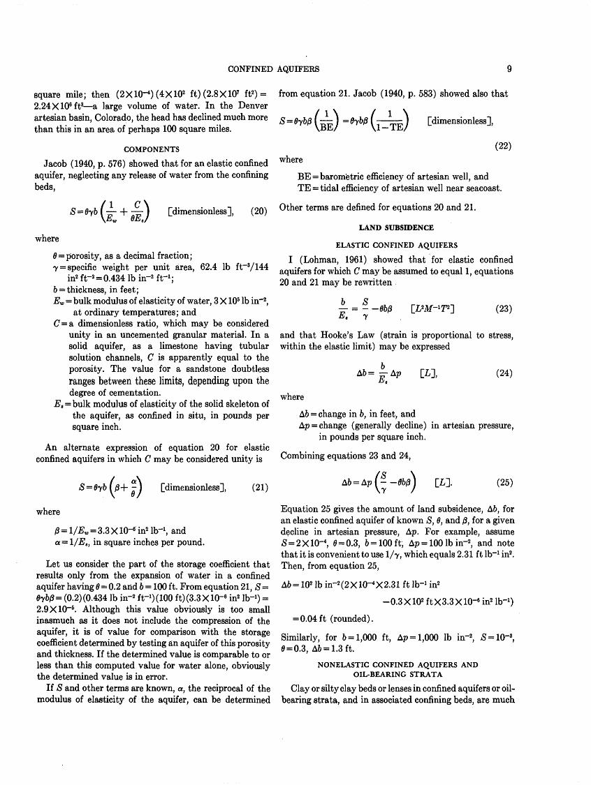
Jacob (1940, p. 576) showed that for an elastic confined aquifer, neglecting any release of water from the confining beds,
( 1 C \ + ) [dimensionless], Ew O&s/
(20)
where
6 = porosity, as a decimal fraction;7 = specific weight per unit area, 62.4 Ib ft"3/ 144
in2 fr2 = 0.4341bin-2 ft-1 ;b = thickness, in feet ;Ew = bulk modulus of elasticity of water, 3 X 10⁵ Ib in"2 ,
at ordinary temperatures; andC = a dimensionless ratio, which may be considered
unity in an uncemented granular material. In a solid aquifer, as a limestone having tubular solution channels, C is apparently equal to the porosity. The value for a sandstone doubtless ranges between these limits, depending upon the degree of cementation.
$8 = bulk modulus of elasticity of the solid skeleton of the aquifer, as confined in situ, in pounds per square inch.
An alternate expression of equation 20 for elastic confined aquifers in which C may be considered unity is
S=( [dimensionless], (21)
where
ft = l/Ew = 3.3 X10⁻⁶ in2 Ib'1 , and a = l/Ea , in square inches per pound.
Let us consider the part of the storage coefficient that results only from the expansion of water in a confined aquifer having 6 = 0.2 and 6 = 100 ft. From equation 21, S = e>ybp= (0.2) (0.434 Ib in-2 ft-1) (100 ft)(3.3X10~6 in2 Ib-1) = 2.9X10"5 . Although this value obviously is too small inasmuch as it does not include the compression of the aquifer, it is of value for comparison with the storage coefficient determined by testing an aquifer of this porosity and thickness. If the determined value is comparable to or less than this computed value for water alone, obviously the determined value is in error.
If S and other terms are known, a, the reciprocal of the modulus of elasticity of the aquifer, can be determined
from equation 21. Jacob (1940, p. 583) showed also that
S = Oybp I ] = Oybft f J [dimensionless],
(22) where
BE = barometric efficiency of artesian well, and TE = tidal efficiency of artesian well near seacoast.
Other terms are defined for equations 20 and 21.
LAND SUBSIDENCE
ELASTIC CONFINED AQUIFERS
I (Lohman, 1961) showed that for elastic confined aquifers for which C may be assumed to equal 1, equations 20 and 21 may be rewritten
£- = - E, 7
(23)
and that Hooke's Law (strain is proportional to stress, within the elastic limit) may be expressed
[L], (24)
where
A6 = change in 6, in feet, andAp = change (generally decline) in artesian pressure,
in pounds per square inch.
Combining equations 23 and 24,
[L]. (25)
Equation 25 gives the amount of land subsidence, A6, for an elastic confined aquifer of known S, 6, and #, for a given decline in artesian pressure, Ap. For example, assume S = 2 X10⁻⁴, B = 0.3, 6 = 100 ft, Ap = 100 Ib in-2 , and note that it is convenient to use 1/7, which equals 2.31 ft Ib"1 in2 . Then, from equation 25,
A6 = 102 Ib in-2 (2X10-4 X2.31 ft Ib-1 in2
-0.3 X102 ft X3.3 X10-6 in2 Ib-1 )
= 0.04ft (rounded).
Similarly, for 6 = 1,000 ft, Ap = 1,000 Ib in~2, S = 1Q-3, 0 = 0.3, A6 = 1.3ft.
NONELASTIC CONFINED AQUIFERS AND OIL-BEARING STRATA
Clay or silty clay beds or lenses in confined aquifers or oil- bearing strata, and in associated confining beds, are much
10 GROUND-WATER HYDRAULICS
TABLE 3. Land subsidence in California oil and water fields
Well field
Wilmington oil field (see Gilluly and Grant, 1949). .. ...........
Water fields: Santa Clara Valley (San Jose) San Joaquin Valley:
Los Banos-Kettleman
Arvin-Maricopa area_
Subsidence (ft)
129
13
26128
Through year
1966
1967
196619621965
1 Stabilized at this amount by repressuring. This figure includes some recovery due to repressuring.
more porous than associated sands or gravels; hence, they contain more fluid per unit volume at a given fluid pressure. When the pressure is gradually reduced, as by discharge of fluids from wells, such beds slowly release fluids and under go nonelastic (plastic), generally irreversible, compaction. (See Athy, 1930; Hedberg, 1936; and Poland and Evenson, 1966.) Compaction of this type is much greater than purely elastic compression, and it has caused appreciable sub sidence of the land surface in both oil and water fields in California, Texas, and elsewhere. Latest available data for several California oil and water fields (J. F. Poland, U.S. Geol. Survey, written commun., Oct. 27, 1967) are given in table 3.
MOVEMENT OF GROUND WATER- STEADY-STATE FLOW
In steady-state flow, hereinafter referred to simply as steady flow, as of ground water through permeable material, there is no change in head with time. Mathe matically, this statement is symbolized by dh/dt = 0, which says that the change in head, dh, with respect to the change in time, dt, equals zero. Steady flow generally does not occur in nature, but it is a very useful concept in that steady flow can be closely approached in nature and in aquifer tests, and this condition may be symbolized by
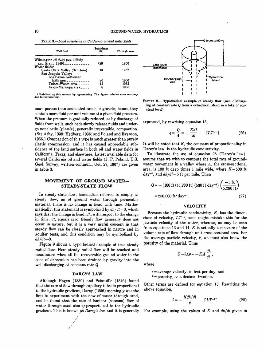
Figure 9 shows a hypothetical example of true steady radial flow. Here steady radial flow will be reached and maintained when all the recoverable ground water in the cone of depression has been drained by gravity into the well discharging at constant rate Q.
DARCY'S LAW
Although Hagen (1839) and Poiseuille (1846) found that the rate of flow through capillary tubes is proportional to the hydraulic gradient, Darcy (1856) seemingly was the first to experiment with the flow of water through sand, and he found that the rate of laminar (viscous) flow of water through sand also is7 proportional to the hydraulic gradient. This is known as Darcy's law and it is generally
Lake level(constant)
Dischargin well
Q (constant) i
^Cylindrical island
FIGURE 9. Hypothetical example of steady flow (well discharg ing at constant rate Q from a cylindrical island in a lake of con stant level).
expressed, by rewriting equation 13,
(26)
It will be noted that K, the constant of proportionality in Darcy's law, is the hydraulic conductivity.
To illustrate the use of equation 26 (Darcy's law), assume that we wish to compute the total rate of ground- water movement in a valley where A, the cross-sectional area, is 100 ft deep times 1 mile wide, where .£ = 500 ft day"1 , and dh/dl = 5 ft per mile. Then
Q= - (100 ft) (5,280 ft) (500 ft day-1 )
= 250,000 ft3 day-1 .
VELOCITY
(27)
Because the hydraulic conductivity, K, has the dimen sions of velocity, LT~l , some might mistake this for the particle velocity of the water, whereas, as may be seen from equations 13 and 14, K is actually a measure of the volume rate of flow through unit cross-sectional area. For the average particle velocity, v, we must also know the porosity of the material. Thus
, dt
where
v = average velocity, in feet per day, and 6 = porosity, as a decimal fraction.
Other terms are defined for equation 13. Rewriting the above equation,
v= Kdh/dl 6
(28)
For example, using the values of K and dh/dl given in
AQUIFER TESTS BY WELL METHODS POINT SINK OR POINT SOURCE 11
equation 27, and assuming 6 = 0.2,
(500 ft day-1 ) (-5 ft/5,280 ft)v 0.2
= 2.4 ft day-1 (rounded). (29)
It should be stressed that the solution of equation 29 is the average velocity and does not necessarily equal the actual velocity between any two points in the aquifer, which may range from less than to more than this value, depending upon the flow path followed. Thus, equation 28 should not be used for predicting the velocity and distance of move ment of, say, a contaminant introduced into the ground.
AQUIFER TESTS BY WELL METHODS- POINT SINK OR POINT SOURCE
STEADY RADIAL FLOW WITHOUT VERTICAL MOVEMENT
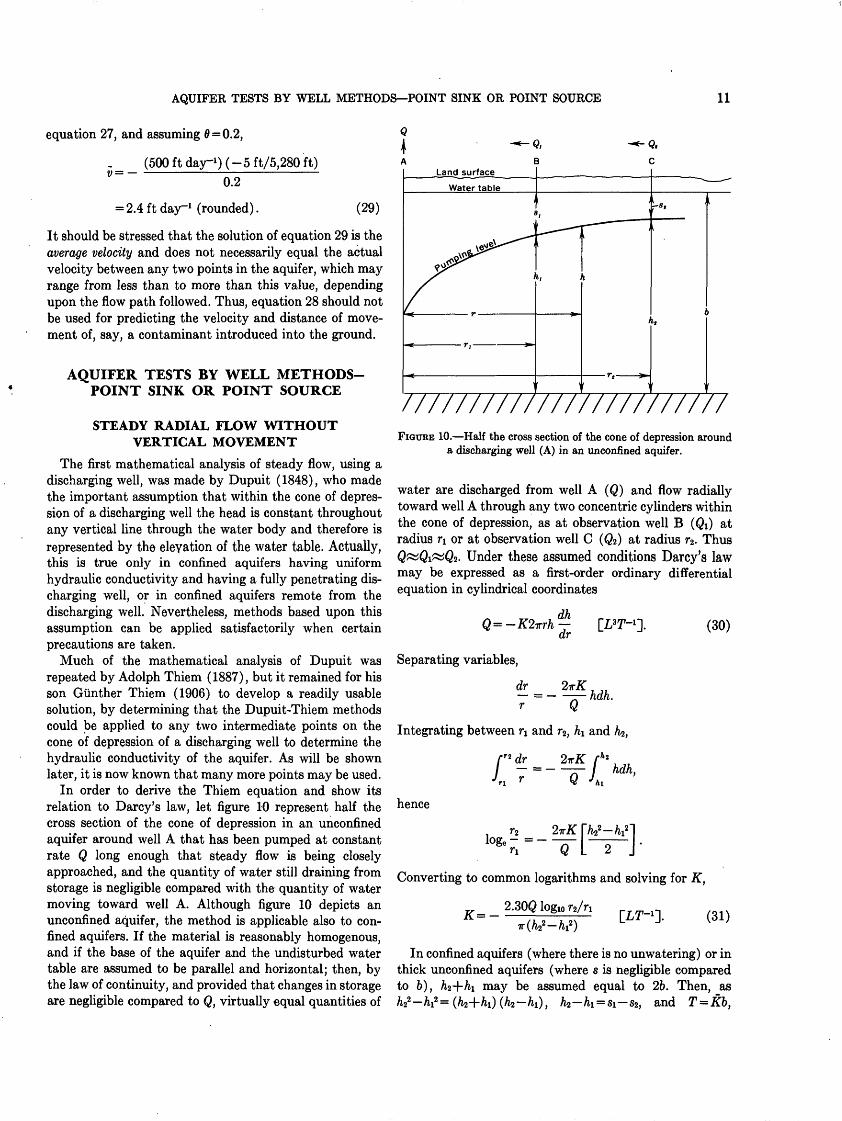
The first mathematical analysis of steady flow, using a discharging well, was made by Dupuit (1848), who made the important assumption that within the cone of depres sion of a discharging well the head is constant throughout any vertical line through the water body and therefore is represented by the elevation of the water table. Actually, this is true only in confined aquifers having uniform hydraulic conductivity and having a fully penetrating dis charging well, or in confined aquifers remote from the discharging well. Nevertheless, methods based upon this assumption can be applied satisfactorily when certain precautions are taken.
Much of the mathematical analysis of Dupuit was repeated by Adolph Thiem (1887), but it remained for his son Gimther Thiem (1906) to develop a readily usable solution, by determining that the Dupuit-Thiem methods could be applied to any two intermediate points on the cone of depression of a discharging well to determine the hydraulic conductivity of the aquifer. As will be shown later, it is now known that many more points may be used.
In order to derive the Thiem equation and show its relation to Darcy's law, let figure 10 represent half the cross section of the cone of depression in an unconfmed aquifer around well A that has been pumped at constant rate Q long enough that steady flow is being closely approached, and the quantity of water still draining from storage is negligible compared with the quantity of water moving toward well A. Although figure 10 depicts an unconfined aquifer, the method is applicable also to con fined aquifers. If the material is reasonably homogenous, and if the base of the aquifer and the undisturbed water table are assumed to be parallel and horizontal; then, by the law of continuity, and provided that changes in storage are negligible compared to Q, virtually equal quantities of
FIGURE 10. Half the cross section of the cone of depression around a discharging well (A) in an unconfined aquifer.
water are discharged from well A (Q) and flow radially toward well A through any two concentric cylinders within the cone of depression, as at observation well B (Qi) at radius n or at observation well C (Q2 ) at radius r2 . Thus Q«Qi«Q2 . Under these assumed conditions Darcy's law may be expressed as a first-order ordinary differential equation in cylindrical coordinates
dr(30)
Separating variables,
dr r Q
hdh.
Integrating between ri and r2 , hi and hz,
dr 2irKQ Jkl
[h * l I "d"1 , J '
hence
Converting to common logarithms and solving for K,
2.30Q logM ra/ri(31)
In confined aquifers (where there is no unwatering) or in thick unconfined aquifers (where s is negligible compared to 6), hi-\-h\ may be assumed equal to 26. Then, as
hi), hz hi = 8i Sz, and T = Kb,

12 GROUND-WATER HYDRAULICS
equation 31 may be rewritten
2.30Qlogw r2/riT=-2ir( 81
(32)
Equations 31 and 32 are forms of the Thiem equation, and later it will be shown how equation 32 can be derived also as a special solution of the nonsteady flow equation.
In thin unconfined aquifers, in which s is an appreciable proportion of 6, Jacob (1963a) showed how to correct the drawdowns (s\ and Sz) to the values that would have been observed had there been no diminution in saturated thick ness (as in a confined aquifer of thickness 6). Note from figure 10 that fo2 = 6 s2 , and hi = b Si. Substituting these values in equation 31 and, for convenience, multiplying both sides of the equation by 26,
K=-
and
T=-
2.30Q logw ra/n
2.30Q logM2ir[(Sl -Si2/26) - ( S2 _
(33)
In equations 32 and 33 note that a straight line should result when values of logio r are plotted at logarithmic scale, against corresponding values of s or s s2/26 at arithmetic scale. Thus, when using semilogarithmic paper, equations 32 and 33 may be written, respectively,
T=- 2.30Q
and
T =
27rAs/Alogio r
2.30Q27rA(s-s2/26)/Alog10 r
(34)
(35)
As or A(s s2/26) is taken over one logio cycle of r, for which Alogio r is 1. Equation 34 is used for tests in confined aquifers.
To my knowledge the first pumping test by the Thiem method made by a member of the U.S. Geological Survey was in 1929 by R. M. Leggette (1936, p. 117-119) at Meadville, Pa., and this may well have been the first one made in the United States. The method was thoroughly investigated and validated in 1931 by Wenzel (1936), who ran two elaborate Thiem tests near Grand Island, Nebr., and by Theis (1932, p. 137-140), who made a test by this method at Portales, N. Mex., in 1931 and two more tests in the same area in 1932 (Theis, 1934, p. 91-95). The fourth locality tested by this method was near Elizabeth City, N.C., by me (Lohman, 1936, p. 42-44) in the spring of 1933. Three additional Thiem tests were made in
Nebraska in the fall of 1933 by Wenzel (1942), and I made an 18-day test, the longest known to me, by this method near Wichita, Kans., in 1937. (See Wenzel, 1942, p. 142- 146; Williams and Lohman, 1949, p. 104-108; Jacob, 1963a, p. 249-254.)
EXAMPLE
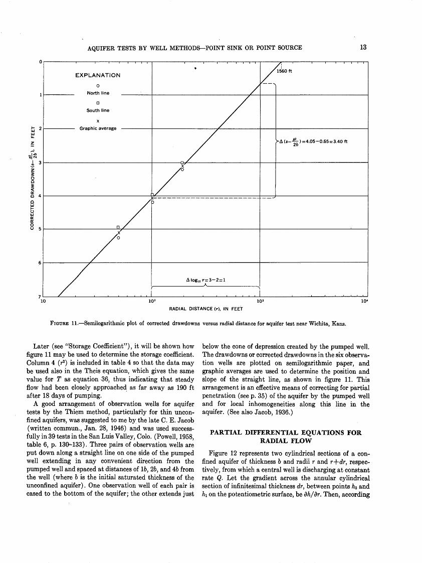
Use of the Thiem method as modified by Jacob for thin unconfined aquifers may be demonstrated from data (table 4) obtained in the 18-day pumping test mentioned above (given in Wenzel, 1942, p. 142; Williams and Lohman,. 1949, p. 104-108; and Jacob, 1963a, p. 249-254). The discharge, Q, was held virtually constant at 1,000±7 gpm for nearly 19 days, when lightening tripped the circuit breaker and stopped the test. The well tapped unconfined alluvial sand and gravel, and the initial saturated thickness, 6, was 26.8 ft. Table 4 gives the data for six observation wells out of a total of 22 at the end of 18 days; three of the wells were on a line extending north from the pumped well, and three were on a line to the south. Wells N-3 and S-3 were planned to be 200 ft from the pumped well, but a property line made it necessary to reduce the distance to 190 ft. Inasmuch as the drawdown correction (s2/26) ranges from about 0.2 to 0.65 ft, it is necessary to use the corrected drawdowns given in the last column. In figure 11, the corrected drawdowns in the six observation wells are plotted on the linear scale against the radial distance on the logarithmic scale, then a straight line is drawn through the three graphic average points (x). Graphic rather than arithmetic averages should be used, because if one of the six drawdown values is spurious for some geologic or other reason, this point may be ignored in drawing the straight line. Note that, although two points determine a straight line, it is much more conforting to have three or more points that fall on or close to a straight line.
Using the slope of the straight line and other data given, T is computed from equation 35 :
T=- (2.30) (1,000 gal min-1 ) (1,440 min day"1 )
(2*0 (7.48 gal ft-3)[- (4.05 ft-0.65 ft)]
= 20,700 ft2 day-1 . (36)
TABLE 4. Data for pumping lest near Wichita, Kans.
Line
North. .....
South......
Well
.. 12 3
.. 12 3
(ft)
49.2100.7 189.4
49.0100.4 190.0
r* (ft»)
2,42010,140 35,900
2,40010,080 36,100
8(ft)
5.914.58 3.42
5.484.31 3.19
sV2& (ft)
0.65.39 .22
.56
.35
.19
8-8V2&(ft)
5.264.19 3.20
4.923.96 3.00
AQUIFER TESTS BY WELL METHODS POINT SINK OR POINT SOURCE 13
EXPLANATION
o
North line
D
South line
Graphic average
1560ft
>-A (s--fr) =4.05-0.65=3.40 ft 20
Alog10 r=3-2=l _____A_____
10 102 103
RADIAL DISTANCE (r), IN FEET
104
FIGURE 11. Semilogarithmic plot of corrected drawdowns versus radial distance for aquifer test near Wichita, Kans.
Later (see "Storage Coefficient"), it will be shown how figure 11 may be used to determine the storage coefficient. Column 4 (r2 ) is included in table 4 so that the data may be used also in the Theis equation, which gives the same value for T as equation 36, thus indicating that steady flow had been closely approached as far away as 190 ft after 18 days of pumping.
A good arrangement of observation wells for aquifer tests by the Thiem method, particularly for thin uncon- fined aquifers, was suggested to me by the late C. E. Jacob (written commun., Jan. 28, 1946) and was used success fully in 39 tests in the San Luis Valley, Colo. (Powell, 1958, table 6, p. 13(M33). Three pairs of observation wells are put down along a straight line on one side of the pumped well extending in any convenient direction from the pumped well and spaced at distances of 16, 26, and 46 from the well (where 6 is the initial saturated thickness of the unconfined aquifer). One observation well of each pair is cased to the bottom of the aquifer; the other extends just
below the cone of depression created by the pumped well. The drawdowns or corrected drawdowns in the six observa tion wells are plotted on semilogarithmic paper, and graphic averages are used to determine the position and slope of the straight line, as shown in figure 11. This arrangement is an effective means of correcting for partial penetration (see p. 35) of the aquifer by the pumped well and for local inhomogeneities along this line in the aquifer. (See also Jacob, 1936.)
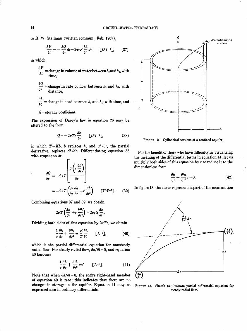
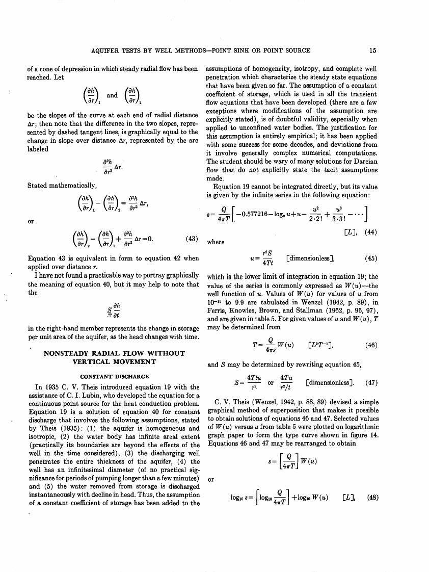
PARTIAL DIFFERENTIAL EQUATIONS FOR RADIAL FLOW
Figure 12 represents two cylindrical sections of a con fined aquifer of thickness 6 and radii r and r+dr, respec tively, from which a central well is discharging at constant rate Q. Let the gradient across the annular cylindrical section of infinitesimal thickness dr, between points hz and hi on the potentiometric surface, be dh/dr. Then, according
14 GROUND-WATER HYDRAULICS
to R. W. Stallman (written commun., Feb. 1967),
dV dQ ,(37)
in which
dV = change in volume of water between h? and hi, with
i time,
dr
dh dt
= change in rate of flow between hz and hi, with distance,
= change in head between hz and hi, with time, and
S = storage coefficient.
The expression of Darcy's law in equation 26 may be altered to the form
Potentiometric surface
Q=-2vTr dr
(38)
in which T = Kb, b replaces h, and dh/dr, the partial derivative, replaces dh/dr. Differentiating equation 38 with respect to dr,
dr dr
FIGURE 12. Cylindrical sections of a confined aquifer.
For the benefit of those who have difficulty in visualizing the meaning of the differential terms in equation 41, let us multiply both sides of this equation by r to reduce it to the dimensionless form
dh d*h 4. r = o.dr dr2
(42)
(39)In figure 13, the curve represents a part of the cross section
Combining equations 37 and 39, we obtain
Dividing both sides of this equation by 2irTr, we obtain
- + = -- [Ir1], (40) r dr dr2 T dt
which is the partial differential equation for nonsteady radial flow. For steady radial flow, dh/dt = Q, and equation 40 becomes
+ -o CL-1 r dr ^ dr* L J(41)
Note that when dh/dt = 0, the entire right-hand member QMof equation 40 is zero; this indicates that there are nochanges in storage in the aquifer. Equation 41 may be FIGURE 13. Sketch to illustrate partial differential equation forexpressed also in ordinary differentials. steady radial flow.
AQUIFER TESTS BY WELL METHODS POINT SINK OR POINT SOURCE 15
of a cone of depression in which steady radial flow has been reached. Let
(*} and (*)VdrA W2
be the slopes of the curve at each end of radial distance Ar; then note that the difference in the two slopes, repre sented by dashed tangent lines, is graphically equal to the change in slope over distance Ar, represented by the arc labeled
Stated mathematically,
dh
Ar. dr2
dh
or
Equation 43 is equivalent in form to equation 42 when applied over distance r.
I have not found a practicable way to portray graphically the meaning of equation 40, but it may help to note that the
in the right-hand member represents the change in storage per unit area of the aquifer, as the head changes with time.
NONSTEADY RADIAL FLOW WITHOUT VERTICAL MOVEMENT
CONSTANT DISCHARGE
In 1935 C. V. Theis introduced equation 19 with the assistance of C. I. Lubin, who developed the equation for a continuous point source for the heat conduction problem. Equation 19 is a solution of equation 40 for constant discharge that involves the following assumptions, stated by Theis (1935): (1) the aquifer is homogeneous and iso tropic, (2) the water body has infinite areal extent (practically its boundaries are beyond the effects of the well in the time considered), (3) the discharging well penetrates the entire thickness of the aquifer, (4) the well has an infinitesimal diameter (of no practical sig nificance for periods of pumping longer than a few minutes) and (5) the water removed from storage is discharged instantaneously with decline in head. Thus, the assumption of a constant coefficient of storage has been added to the
assumptions of homogeneity, isotropy, and complete well penetration which characterize the steady state equations that have been given so far. The assumption of a constant coefficient of storage, which is used in all the transient flow equations that have been developed (there are a few exceptions where modifications of the assumption are explicitly stated) , is of doubtful validity, especially when applied to unconfined water bodies. The justification for this assumption is entirely empirical; it has been applied with some success for some decades, and deviations from it involve generally complex numerical computations. The student, should be wary of many solutions for Darcian flow that do not explicitly state the tacit assumptions made.
Equation 19 cannot be integrated directly, but its value is given by the infinite series in the following equation:
- 4-|[-0.577216-log. U+U- £, + ^, -.
where
u= [dimensionless],TC./ t
(44)
(45)
which is the lower limit of integration in equation 19; the value of the series is commonly expressed as W(u) the well function of u. Values of W(u) for values of u from 10-15 to 9.9 are tabulated in Wenzel (1942, p. 89), in Ferris, Knowles, Brown, and Stallman (1962, p. 96, 97), and are given in table 5. For given values of u and W(u), T may be determined from
47TS
and S may be determined by rewriting equation 45,
S=
(46)
or [dimensionless]. (47)/ / / fc
C. V. Theis (Wenzel, 1942, p. 88, 89) devised a simple graphical method of superposition that makes it possible to obtain solutions of equations 46 and 47. Selected values of W(u) versus u from table 5 were plotted on logarithmic graph paper to form the type curve shown in figure 14. Equations 46 and 47 may be rearranged to obtain
,= uor
Iogi0 s =
W(u)
-^- +log10 TF(W ) [L], (48)
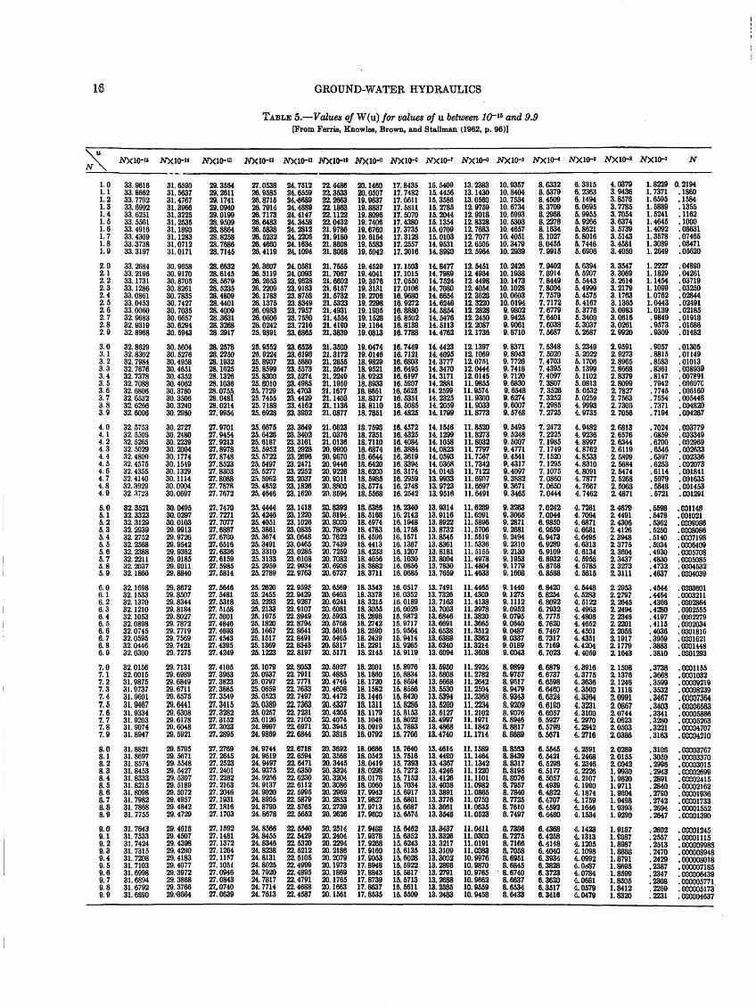
GROUND-WATER HYDRAULICS
TABLE 5. Values of W(u) for values of u between 10~u and 9.9 [From Ferris, Knowles, Brown, and Stallman (1962, p. 96)]
1.01.11.21.31.41.51.61.71.81.9
2.02.12.22.32.42.52.62.72.82.9
3.03.13.23.33.43.53.63.73.83.9
4.04.14.24.34.44.54.64.74.84.9
5.05.15.25.35.45.55.65.75.85.9
6.06.16.26.36.46.56.66.76.86.9
7.07.17.27.37.47.57.67.77.87.9
8.08.18.28.38.48.58.68.78.88.9
9.09.19.29.39.49.59.69.79.89.9
2VX10-"
33. 961633.866233. 779233.699233. 625133. 556133. 491633. 430933.373833.3197
33. 268433. 219633. 173133. 128633. 086133. 045333.006032. 968332. 931932.8988
32. 862932. 830232. 798432. 767632. 737832. 708832.680632. 653232. 626632.6006
32. 575332. 550632. 526532. 502932. 480032. 457532. 435532. 414032. 392932. 37'.>3
32. 352132. 332332. 312932. 293932. 275232.256832.238832. 221132. 203732.1866
32. 169832. 153332. 137032. 121032. 105332. 089832. 074532.059532. 044632.0300
32.015632. 001531. 987531. 973731.960131.946731. 933431. 920331. 907431. 8947
31. 882131. 869731. 857431. 845331. 833331. 821531. 809831. 798231. 786831. 7755
31. 764331. 753331. 742431. 731531. 720831. 710331. 699831. 689431.679231.6680
JW*.
31. 658031.563731. 476731.396631.322531.253531. 188031.128331.071231.0171
30. 965830. 917030. 870530. 826130.783530.742730. 703530.665730.629430.5943
30. 560430. 527630.495830. 465130. 435230. 406230.378030. 350630. 324030.2980
30. 272730.248030.223930.200430. 177430. 151930. 132930. 111430.090430. 0697
30.049530.029730.010329.991329.972629.954229. 936229. 918529.901129.8840
29.867229.850729.834429.818429.802729. 787229. 771929. 756929. 742129. 7275
29. 713129. 698929.684929. 671129. 657529.644129.630829. 617829.604829. 5921
29. 579529.567129.554829.542729. 530729. 518929.507229. 495729.484229.4729
29. 461829.450729.439329.42VO29. 418329. 407729. 397229.386829.376629.3664
WX.O-.
29.368429.261129. 174129.094029.019928.950928.886428.825823.768628. 7145
28.683228.614528.567928.523528.480928.440128.400928.363128.326828.2917
28.257828.225023.193228. 162528.132628.103828.075528.048128. 021427.8954
27. 970127.945427.921327.897827. 874827.852327.830327.808327. 787827. 7672
27. 747027.727127. 707727.688727.670027.651627.633627.615927.598527.5814
27.564627.548127.531827.515827.500127.484627.469327.454327.439527.4249
27. 410527.396327.382327.368527.354927.341527.328227.315227.302327.2896
27.276927.264527.252327.240127.228227.216327.204627. 193127. 181627. 1703
27. 159227. 148127. 137227.126427. 115727. 105127.094627.084327,074027.0839
.WXio-18
27.053826.958528.871626. 791426. 717326.648326.583826.523226.466026.4119
26.360726. 311928.265326.220926.178328. 137526.098326.060626.024225. 9891
25. 955225. 922425.880725.859925.830025.801025.772925. 745525. 718825. 6928
25.667525.642325. 618725. 595225. 672225. 549725.527725. 506225.485225.4646
25.444425.424625.405125.386125.367425. 349125. 331025. 313325.295925. 2789
25.262025.245525.229325.213325. 197525.182025.166725. 151725. 136925.1223
25. 107925.093725.079725. 065925.052325.038925.025725.012624.999724.9869
24.974424.961924.949724.937524. 925624. 913724.802024.880524. 878024. 8678
24.856624.845524. 834624.823824. 813124.802524.792024. 781724. 771424. 7613
wax
24. 751224.655924<668924.488924. 414724.345824.281224.220824.163424.1094
24.058124.009323.982823.918323.876823.834923. 795723.758023. 721623.6865
23.652323.619823.588023. 557323.527423.498523.470323.442923.416223.3802
23.364923.340223.316123.292623.269823.247123.225223.203723.182623.1620
23. 141823.122023.102623.083523.064823.046523.028523. 010822.993422.9763
22. 959522.942922.928722.910722. 894922.879422.864122.849122.834322.8197
22.805322. 791122. 777122.763322. 749722.736322.723122.710022.697122.6844
22. 671822.659422.647122.635022.623022. 611222.599522.587922. 576522.6652
22.654022.542922.532022. 521222. 510522.499922.489522. 479122.468822.4587
JMM
22.448822.353322.266322.186322.112222.043221. 978621.918021.860821.8063
21. 755621. 706721.660221. 615721. 573221.632321.493121.456421.418021.3830
21.360021.317221.285521.254721.224921. 195921. 167721.140321. 113621.0877
21.062321.037621.013620.990020.987020.944620.922620.801120.880020.8594
20.839220.819420.808020.780920.762220.743920.725920. 708220.680820.6737
20.656920.640320.624120.608120.592320.576820.561620.546520.631720. 5171
20.602720.488520.474620.460820.447220.433720.420520.407420.394520.3818
20.369220.356820.344520.332420.320420.308620.296920.285320.273920.2628
30.251420.240420.229420.218620.207920. 197320.186920. 176520.166320.1581
tfXKH,
20.146020.050719.963719.883719.809819.740819.676019. 616419.658319.5042
19.452919.404119.357619.313119.270619.229819. 180519. 152819. 116419.0813
19.047419.014618.982918. 952118. 922318.893318. 865118.837718.811018. 7851
18. 759818. 735118. 711018. 687418.664418.642018.620018. 593518. 677418.5683
18.636818. 516818.497418.478318. 459618. 441318.423318.405618. 388218. 3711
18.354318. 337818. 321518. 305518. 289818. 274218.258018.243918.229118. 2145
18.200118.186018. 172018. 158218. 144618. 131118. 117918. 104818.091918.0792
18.088818.054218.041918. 029818.017818.006017.994317. 982717. 971317.9800
17.948817.937817.928817. 916017.805317. 894817.884317. 873917.863717.8535
WOM
17. 843517. 748217. 661117.681117. 607017.438017.373517.312817. 255717. 2016
17.150317. 101517.055017.010616.988016. 927216.883016.850216.813816. 7788
16.744916. 712116.680316. 649516.619716. 580716. 662516. 635116. 508516.4825
16.457216. 432516.408416.388416.361916.339416. 317416. 295916. 274816.2542
16.234016. 214216. 194816. 175816. 157116. 138716. 120716. 103016. 085616.0885
16. 051716.035216. 018916.002915. 987215. 971715.956416. 941415. 926515. 9119
15. 897615.883415. 869415. 855615.842015.828615. 815315.802215. 789316. 7766
15.764015. 751615. 739315. 727215. 715215. 703415. 691715.680115.668715.6574
15.646215. 635215. 624315. 613515.602315. 592215. 581716. 571315. 681115.5509
max
15.540915. 445615.358615. 278515.204415. 135415.070915.010314.9531148980
14.847714. 798914. 752414. 708014.665414.624614.585414. 547614. 511314.4762
14.442314. 409514. 377714. 347014.317114.288114. 259914. 232514. 2059141799
14. 154814.129914. 105814,082314.059314. 036814.014813.993313. 972313. 9516
13.931413. 911613. 892213. 873213.854513. 836113. 818113.800413.783013. 7659
13. 749113. 732613. 716313.700313.884613. 669113.653813.638813.624013.6094
13. 695013.580813.566813.653013.639413.528013. 512713. 499713.486813.4740
13. 461413.448013.436713.424613. 412613.400813. 388113.377613.366113.3548
13.343713.332813. 321713.310913.300213.288813. 279113.263813.268613.2433
DX1M
13.238313. 143013.056012. 975912. 801812.832312.768312. 707712. 650512.5984
12. 645112.488412.449812.406412. 362812.322012.282812.245012.208712. 1736
12. 139712. 106912.075112.044412.014511. 985511. 957411.930011.903311.8773
11.852011. 827311.803211. 779711. 756711. 734211.712211.690711. 669711. 6491
11.628911.609111.589811.570611. 551911. 533611. 515511. 497811.480411.4633
11. 446511.430011. 413811.397811.382011.366511.351211. 336211.321411.3608
11.292411. 278211.264211.250411.236811.223411. 210211. 197111. 184211.1714
11.158911.146411. 134211.122011. 110111.098211.086611.075011.083511.0523
11.041111.030011.019111.008310.997610.987010. 976510.886210.956910.9458
JVX.O-.
10. 935710.840410.753410. 673410. 599310.630310.465710. 405110. 347910.2939
10.242610.193310. 147310. 102310.060310.01949.98029.94259.90619.8710
9.83719.80439.77269. 74189.71209.68309.65489.62749.60079.5743
9.54959.52489.60079. 47719.46410.43179. 40979.38829.36719.3465
9.32839.30859.28719.26819.24949.23109.21309.19539. 17799.1608
9.14409.12759. 11129. 09529. 07959.06409.04879.03379.01899.0043
8.9899a 97678.98178.94798.93438.92098.80768.89468.88178.8689
a 85338.8439a 8317a 8195a 8076a 79578.78408.77258. 76108. 7497
a 73868.7275a 71688.7058a 69518.63458.67408.66378.65348.6433
wax
8.63328.53798.45098.37098.28888.22788.16348.10278.04557.9915
7.94027.89147.84497.80047. 75797. 71727. 67797.64017.60387.6687
7.53487.50207. 47037. 43957.40977.38077. 35267.32527.29857.2725
7.24727.22257. 19857. 17497.15207.12957. 10757.08607.06507.0444
7.02427.00446.98506.98596.94736.92896.91096.89326.87586.8688
6.84206.82546.80926. 79326. 77756.76206. 74676. 73176. 71696.7023
6.68796. 67376. 65986.64606.63246.61906.60576.59276. 57986.6671
6.55456.54216.52986. 51776.50576.49396.48226.47076. 45926.4480
6.43686.42586.41486.40406.39346.38286.37236.36206.35176.3416
wax »
6. 33156.23636.14946.06955.99555.92666.86215.80165. 74465.6906
6.63946.59075.54435.49996. 45755. 41676.37765.34005.30376.2687
5.23495.20225. 17065.13995. 11025.08135.05325. 02594.999349735
4.94824.92364.89974.87624.85334.83104.80914. 78774.76674. 7462
47281470844.68714668146495 :4.63134 61344.59534578546616
4644845283 .4512244963448064.46524.4501 !4.4351 ,4.4204 !44059
43916437754.36364.3500433644.32314.31004. 2970 !4.28424 2716 !
4.259142468 '4.23464.22264 2107419804 1874417594164641534
414234 13134120541098409924088740784408314057940479
X10-»
i.03793.94363.85763.77853.70643.63743. 57393.51433.45813.4050
3.35473.30693.26143. 21793.17633. 13653.09333.06163.02612.9920
2.95912.92732. 89652.86682.83792.80992.78272.75632.73062.7068
2.68132. 65762.63442.61192.58992.56842.64742.52632.60632.4871
2.46792.44912.43082.41262.39482.37752.36042.34372.32732.3111
2.29532.27972.28452.24942.23462.22012.20582.19172.17792.1643
2.15082.13762.12462.11182.09912.08672.07442.08232.06032.0386
2.02892.01552.0042.9930.9820.9711.9804.9498.9393.9280
.9187
.8087
.8987
.8888
.8791
.8695
.8599
.8505
.8412
.8320
2VTX10-'
1.82291. 73711.65951.68891.62411.46451.40921. 35781.30891.2649
1.22271.18291.14541.10991.07621.04431.0139.9849.9573.9309
.8057
.8815
.8583
.8361
.8147
.7942
.7745
.7554
.7371
.7194
,7024.6859.6700.6546.6397.6253.6114.5979.5848.6721
.5698
.5478
.5362
.5250
.5140
.5034
.4930
.4830
.4732
.4637
.4544
.4464
.4368
.4280
.4197
.4115
.4036
.3959
.3883
.3810
.3738
.3663
.3599
.3532
.3467
.3403
.3341
.3280
.3221
.3163
.3108
.3050
.2986
.2943
.2891
.2840
.2780
.2742
.2694
.2647
.2602
.2557
.2513
.2470
.2429
.2387
.2347
.2308
.2269
.2231
N
0. 2194.1860.1584.1355.1162.1000.08631.07465.08471.05620
.04890
.04261
.03719
.03250
.02844
.02491
.02185
. 01918
.01686
.01482
.01305
.01149
. 01013
.008939
. 007891
.00697C
.006160
.005448
.004820
.004267
.003779
.003349
.002969
.002633
.002336
.002073
.001841
.001635
.001453
.001291
.001148
.001021
.0008086
.0008086
.0007198
.0008409
.0005708
.0005085
.0004532
.0004039
.0003601
.0003211
.0002864
.0002555
.0002279
.0002034
.0001810
.0001621
.0001448
.0001293
.0001155
.0001032
.00009219
.00008239
! 00008583.00005886.00005263.00004707.00004210
.00003767
.00003370
.00003015
.00802699
.08002415
.00002162
.00001936
.00001733
.00001552
.00801390
.00001245
.00001115
.000009988
.000008948
.000008018
.000007185
' 080005771! 008005173'.080004637
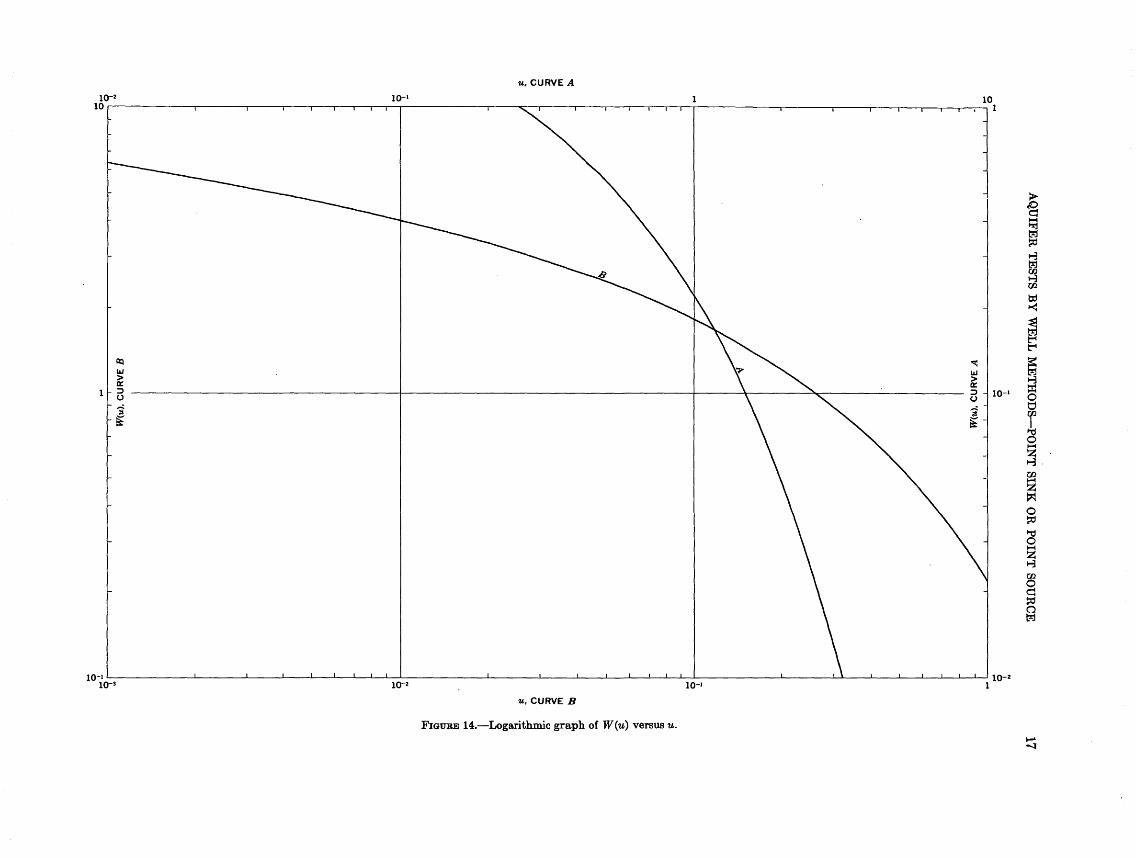
AQ
UIFE
R T
EST
S BY
WE
LL
ME
TH
OD
S P
OIN
T SIN
K O
R PO
INT
SOU
RC
E17

18 GROUND-WATER HYDRAULICS
log,0rV<
Data plot
log 10 -
Type-curve plot
log, 0 M
FIGURE 15. Relation of W(u) and u to s and r*/t, and displacements of graph scales by amounts of constants shown.
and
or
r2
logic T = +logio u (49)
If the discharge, Q, is held constant, the bracketed parts of equations 48 and 49 are constant for a given pumping test, and W(u) is related .to u in the manner that s is related to rz/t, as shown graphically in figure 15. Therefore, if values of s are plotted against rz/t (or l/t if only one observation well is used) on logarithmic tracing paper to the same scale as the type curve, the data curve will be similar to the type curve except that the two curves will be displaced both vertically and horizontally by the amounts
of the bracketed constants in equations 48 and 49. The data curve is superimposed on the type curve, and a fit, or near fit, is obtained, keeping the coordinate axes of the two curves parallel. An arbitrary match point is selected any where on the overlapping parts of the two sheets, the four values of which (two for each sheet) are then used in solving equations 46 and 47. It is convenient to choose a point whose coordinates on the type curve are both unity that is, where W(u) = 1.0 and u = 1.0. In some plots it may be desirable to use a power of 10 for one coordinate. (See fig. 16.)
A convenient alternative method is to plot W(u) versus l/u as the type curve; then for the data curve, s may be plotted against t/rz (or t, if only one observation well is used). This procedure is illustrated on plate 9, which also may be used for solutions of the Theis equation by superposing plots of t/r2 or t versus s on the heavy parent type curve.
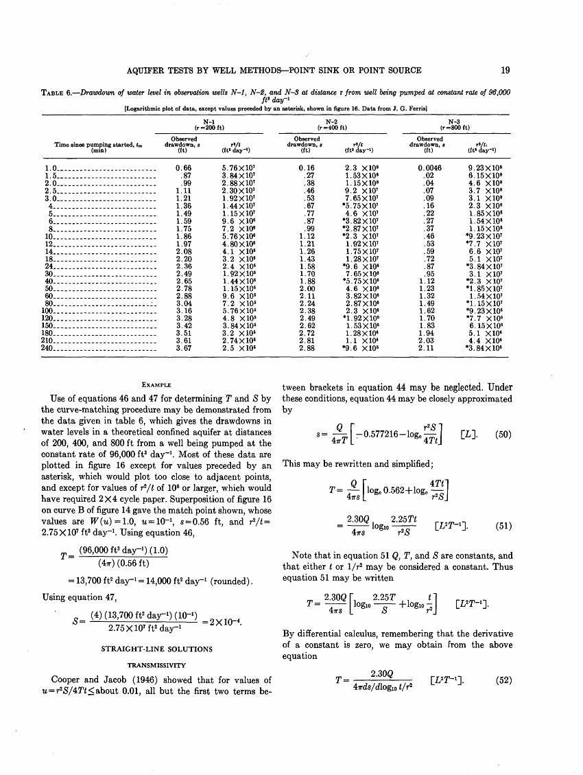
AQUIFER TESTS BY WELL METHODS POINT SINK OR POINT SOURCE 19
TABLE 6. Drawdown of water level in observation wells N-l, N-2, and N-S at distance r from well being pumped at constant rate of 96,000ft* day~l
[Logarithmic plot of data, except values preceded by an asterisk, shown in figure 16. Data from J. G. Ferris]
Time since pumping started, tm (mm)
1.0 . 1.5 .- - _2.0.........................2.5 _- 3.0...- ..................4... ........... ............5 6..........................8..--....-.----.-..-.-.....
10-. .............. .........12..........................14........--.-..-.--......-.18..-.------.--.-.-.-.......24..........................30-.. ............. .........40-.-.........--....-...-...50.--.-.-----...------..--..60.--.-.--------..-.---.....80..-..--------........-...;
100-.. ..................... .120.-..---...--.-----....-...150........-.----....-.....-.ISO..-.....--------.--....-..210---.....-....-....-....-..240 ....... ........... ..
(r
Observed drawdown, «
(ft)
0.66.87.99
1.111.211.361.491.591.751.861.972.082.202.362.492.652.782.883.043.163.283.423.513.613.67
N-l =200 ft)
rV« (ft« day1)
5.76X1073.84X1072.88X1072.30X1071.92X1071.44X1071.15X1079.6 XlO67.2 XlO85.76X1084.80X1084.1 XlO63.2 XlO82.4 XlO61.92X1061.44X1061.15X1069.6 XlO67.2 XlO55.76X1054.8 XlO63.84X1083.2 XlO62.74X1062.5 XlO6
(r
Observed drawdown, a
(ft)
0.16.27.38.46.53.67.77.87.99
1.121.211.261.431.581.701.882.002.112.242.382.492.622.722.812.88
N-2 =400 ft)
r'A (ft» day-')
2.3 XlO81.53X1081. 15X10"9.2 XlO77.65X107
'5.75X1074.6 XlO7
*3.82X107*2.87X107*2.3 XlO71.92X1071.75X1071.28X107
*9 6 XlO67.65X106
'5.75X1064.6 XlO63.82X1062.87X1062.3 XlO6
*1.92X1061.53X1081.28X1061.1 XlO6
*9.6 XlO5
(r
Observed drawdown, a
(ft)
0.0046.02.04.07.09.16.22.27.37.46.53.59.72.87.95
1.121.231.321.491.621.701.831.942.032.11
N-3 =800 ft)
r«/t, (ft« day'1 )
9.23X10"6.15X10"4.6 XlO83.7 XlO83.1 X10"2.3 X10"1.85X1081.54X10"1.15X10"
*9.23X107*7.7 XlO76.6 XlO75.1 XlO7
'3.84X1073.1 XlO7
*2.3 XlO7*1.85X1071.54 XlO7
"1.15X107*9.23X106*7.7 XlO66.15X1065.1 XlO64.4 XlO6
*3.84X106
EXAMPLE
Use of equations 46 and 47 for determining T and S by the curve-matching procedure may be demonstrated from the data given in table 6, which gives the drawdowns in water levels in a theoretical confined aquifer at distances of 200, 400, and 800 ft from a well being pumped at the constant rate of 96,000 ft3 day"1 . Most of these data are plotted in figure 16 except for values preceded by an asterisk, which would plot too close to adjacent points, and except for values of r*/t of 108 or larger, which would have required 2X4 cycle paper. Superposition of figure 16 on curve B of figure 14 gave the match point shown, whose values are W(u) = l.Q, u=W~l, s = 0.56 ft, and r*/t = 2.75XlO7 ft2 day-1 . Using equation 46,
T = (96,000 ft3 day1 ) (1.0) (4*0 (0.56 ft)
= 13,700 ft2 day-1 = 14,000 ft2 day-1 (rounded).
Using equation 47,
' (4) (13,700 ft2 day-1 ) (10-1 ) _ 9vtn_4 2.75XlO7 ft2 day-1 " X U '
STRAIGHT-LINE SOLUTIONS
TRANSMISSIVITY
Cooper and Jacob (1946) showed that for values of u = r*S/4Tt< about 0.01, all but the first two terms be
tween brackets in equation 44 may be neglected. Under these conditions, equation 44 may be closely approximated by
S = 4-^[-0.577216-log.gJ
This may be rewritten and simplified;
T= ^-
(50)
.562+loge 4̂ ]
(51)
Note that in equation 51 Q, T, and S are constants, and that either t or 1/r2 may be considered a constant. Thus equation 51 may be written
2.30Q 2.257
By differential calculus, remembering that the derivative of a constant is zero, we may obtain from the above equation
2.30Qt/r2 (52)
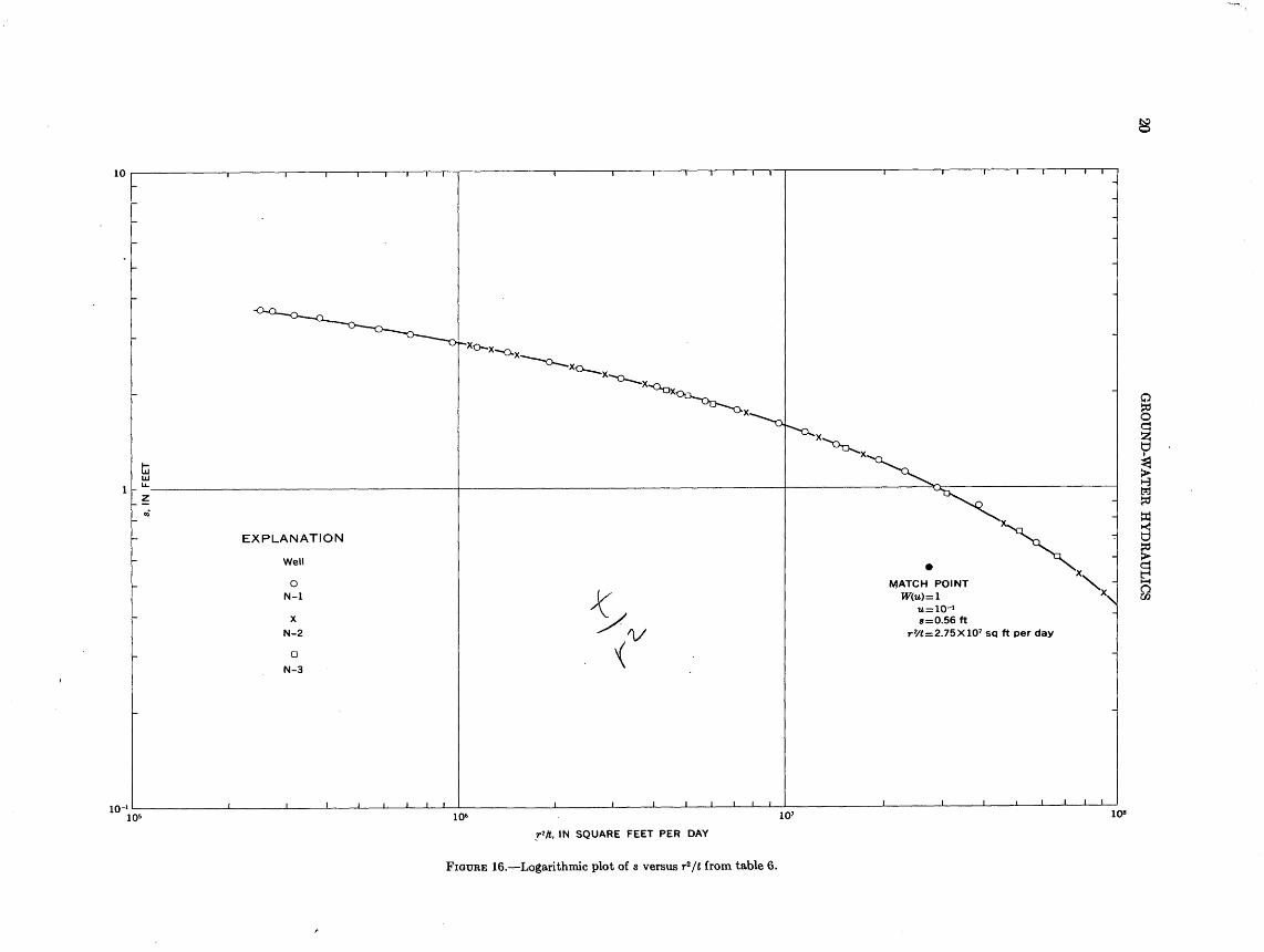
20G
RO
UN
D-W
AT
ER
HY
DR
AU
LIC
S
'S bO
AQUIFER TESTS BY WELL METHODS POINT SINK OR POINT SOURCE 21
Similarly, considering also r as a constant,
2.30QT =t
(53)
Considering t as a constant,
2.30Q 2.30Q1/r2 (54)
As the relation of s to the log terms is linear on semi- logarithmic plots, we may change from infinitesimals (derivatives) to finite values, whence equations 52 though 54 become, respectively,
/TT __
m __
2.30Q
and
47rAs/Alogio t/r*
2.30Q4irAs/Alogio t
2.30Q
2?rAs/Alogio f
(55)
(56)
(57)
Note that equation 57, obtained by simplification and differentiation of equation 51 for nonsteady flow, is identical to equation 34 the steady flow, or Thiem, equation for confined aquifers or for relatively thick unconfined aquifers. In testing relatively thin unconfined aquifers, equation 35, which contains Jacob's drawdown correction, should be used rather than equations 34 or 57, for reasons given earlier.
Equations 55 through 57 are readily solved using semi- logarithmic paper, by plotting values of s on the linear scale against corresponding values of the log terms on the logarithmic scale and determining the value of As for one log cycle. Figure 11 illustrates the method.
For preparing a composite graph for several observation wells and several wells being pumped at constant but different rates, Qi, Qz, Qa, and so on, the following equation may be used:
T = 2.30(58)
In using equation 58 for, say, three pumping wells within an area of overlapping cones of depression, values of Si/Qi, ti/riz ; Sz/Qz, tz/rzz ; and ss/Qs, t3/rs2 are plotted on the same semilogarithmic graph, and, if u is less than or equal to 0.01 for all values, all points should fall on or near a straight line and may be used in determining a single set of values of T and S for the entire well field.
Cooper and Jacob (1946) used r2/t rather than t/rz in
equations 55 and 58, whence a minus sign preceded the right-hand sides of their equations and the slope of the straight line was reversed.
STORAGE COEFFICIENT'
In plotting data for the straight-line solutions of equations 52 through 54, it is convenient to consider the top of the arithmetic scale as the line of zero drawdown, as shown on figure 11. The drawdown then increases down ward, as in the well. Cooper and Jacob (1946) showed that by extending the straight line until it intersects the line of zero drawdown, and noting the value of t, t/r2 , r2/t, or r at the point of intersection, the storage coefficient can be determined as follows. At zero drawdown, from equation 50,
0
= 0.577216 = loge 1.781,
= 1.781,r2S
and
(at point of zero drawdown). (59)
Equation 59 gives the desired result satisfactorily if the straight line has sufficient slope so that its zero arithmetic coordinate can be found within the confines of the plot, as in figure 11. However, if the slope is nearly flat, so that the zero arithmetic coordinate occurs outside the confines of the plot, error may result from graphical extrapolation onto an adjoining sheet of graph paper. In order to avoid such errors, I described the following method (Lohman, 1963) for determining S within the data region of straight-line plots without the need for mechanical extrapolation. Equation 51 may be rewritten
o _ 2.
log10-1 [47r71s/2.30Q] '(60)
Combining equations 55 and 60 for the value of As for one logio cycle of t/r2 (unity), we obtain
S=- 2.25 TV/r2(61)
Note that in equation 61 the values of T, s, and As are the same as those used in equations 55 and 56 for determining T. For equations 57 and 58, the comparable equations for
22 GROUND-WATER HYDRAULICS
S are, respectively,
2.257V/r2logio-1[-2s/As]
for plots of s versus r and
2.1
(62)
(63)
for plots of s/Q versus t/r2.
EXAMPLE
Note in figure 11 that the extrapolated straight line reaches the line of zero drawdown at r= 1,560 ft. Using equation 59 and the results of the Thiem test accompany ing figure 11,(2 -25)(2°'7)(i8days) =o.35
(1,560ft) 2
Similarly, using equation 62,
0 (2.25) (20,700 ft2 day-1 ) (18 days)/(100 ft) 2logio-1[-2(-4.05/3.40)]
83.9 83.9Iogi0-1 [2.38235] 241.19
= 0.35 (rounded).
Note that in the final bracketed denominator .38235 is the mantissa, which determines the digits 24119, and that the 2. is the characteristic, which determines the three digits to the left of the decimal point, giving the final antilog as 241.19.
Jacob (1963a, p. 247) showed that in thin unconfined aquifers, such as the one tested near Wichita, Kans., a drawdown correction must be applied in solving for both T and S. The correction to be applied to S (after the drawdowns have been corrected) is
'-(59* (64)
where
S' is the corrected value; b, for the Wichita test, was 26.8 ft; and s, for the Wichita test at the geometric mean distance
of 100 ft, was 4.5 ft.
Hence,
(rt/» o _ A c\
' ' ) 0.35 = 0.29 = 0.3 (rounded). 26.8 /
PRECAUTIONS
Although the straight-line solutions described above give very satisfactory results when properly used, it is un
fortunately true that they have been improperly applied by many workers. It was stated in their derivation that they can be used only when u is less than or equal to about 0.01, but the importance of this seemingly has been forgot ten all too often. Let us consider the several parameters involved in this criterion by reexamining equation 45:
u = _ 47V
and letting u be less than or equal to about 0.01.First note that because S appears in the numerator
(other things being equal including time, t), the value of u is considerably greater for an unconfined aquifer of specific yield from 0.1 to 0.3 than for a confined aquifer whose storage coefficient may range from only say 10~5 to 10~3 . To compensate for this, t must be greater by several orders of magnitude in testing an unconfined aquifer than in testing a confined aquifer. Equally important is the fact that pumping time in an unconfined aquifer must be long enough to allow reasonably complete drainage of material within that part of the cone of depression being observed. On the contrary, release of water from a reasonably elastic confined aquifer not unwatered during testing is virtually instantaneous.
Note that r appears as rz in the numerator. Thus, other things being equal, the greater the distance r, the longer t must be to allow u to reduce to the required maximum value.
In the denominator, 4 and T are constants, but again, other things being equal, the smaller the value of T, the more time is required for u to reduce to 0.01 or less.
For a given array of wells in a particular aquifer, assuming that sufficient pumping time is allowed to ade quately drain the cone of depression in an unconfined aquifer, all parameters except t are constants; therefore pumping time generally is the only control for reducing u to or below its maximum permissible value, and this is the parameter generally neglected by many.
In a drawdown-time test (s versus Iog10 1 or Iog10 t/r2), data points for any particular distance r will begin to fall on a straight line only after the time, t, is sufficiently long to satisfy the above criteria. In a drawdown-distance test (s versus logic r, Thiem test), the well must be pumped long enough that the data for the most distant observation will satisfy the requirements; then only the drawdowns at or after this value of t may be analyzed on a semilogarithmic plot for one particular value of t.
Equation 56 may be used for a time-drawdown or time- recovery test on a pumped well in a confined aquifer or in an unconfined aquifer that drains rapidly and reasonably completely during the test. When properly used, equation 56 gives the same results as the more complicated recovery equation of Theis (1935). In an unconfined aquifer that drains very slowly or incompletely or both, however, the
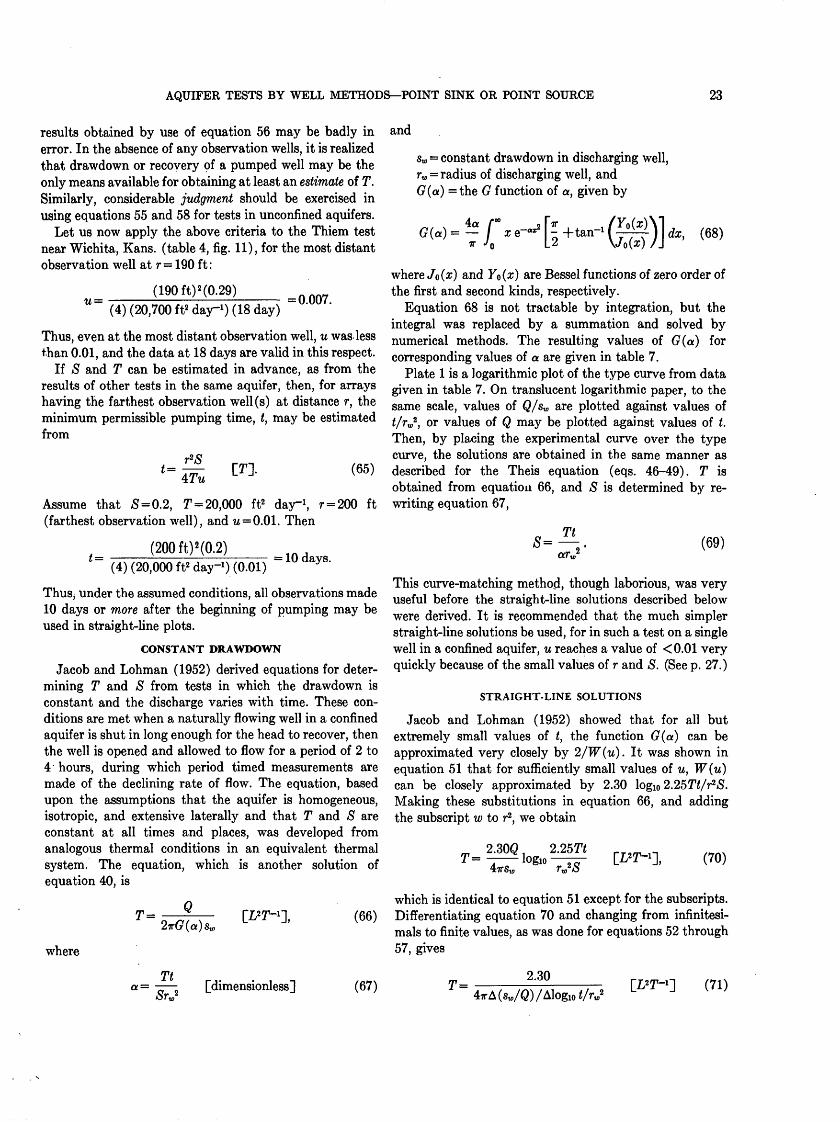
AQUIFER TESTS BY WELL METHODS POINT SINK OR POINT SOURCE 23
results obtained by use of equation 56 may be badly in error. In the absence of any observation wells, it is realized that drawdown or recovery of a pumped well may be the only means available for obtaining at least an estimate of T. Similarly, considerable judgment should be exercised in using equations 55 and 58 for tests in unconfined aquifers.
Let us now apply the above criteria to the Thiem test near Wichita, Kans. (table 4, fig. 11), for the most distant observation well at r= 190 ft:
and
u = (190 ft) 2 (0.29)(4) (20,700 ft2 day-1 ) (18 day)
= 0.007.
Thus, even at the most distant observation well, u was less than 0.01, and the data at 18 days are valid in this respect.
If S and T can be estimated in advance, as from the results of other tests in the same aquifer, then, for arrays having the farthest observation well(s) at distance r, the minimum permissible pumping time, t, may be estimated from
(65)
Assume that S = 0.2, T = 20,000 ft2 day-1 , r = 200 ft (farthest observation well), and w = 0.01. Then
(200ft) 2 (0.2)(4) (20,000 ft2 day-1 ) (0.01)
= 10 days.
Thus, under the assumed conditions, all observations made 10 days or more after the beginning of pumping may be used in straight-line plots.
CONSTANT DRAWDOWN
Jacob and Lohman (1952) derived equations for deter mining T and S from tests in which the drawdown is constant and the discharge varies with time. These con ditions are met when a naturally flowing well in a confined aquifer is shut in long enough for the head to recover, then the well is opened and allowed to flow for a period of 2 to 4 hours, during which period timed measurements are made of the declining rate of flow. The equation, based upon the assumptions that the aquifer is homogeneous, isotropic, and extensive laterally and that T and S are constant at all times and places, was developed from analogous thermal conditions in an equivalent thermal system. The equation, which is another solution of equation 40, is
T = Q
where
a=Tt
= [dimensionless]
(66)
(67)
sw constant drawdown in discharging well, rw = radius of discharging well, and (7 (a) =the G function of a, given by
where JQ(X) and Y0 (x) are Bessel functions of zero order of the first and second kinds, respectively.
Equation 68 is not tractable by integration, but the integral was replaced by a summation and solved by numerical methods. The resulting values of G(a) for corresponding values of a are given in table 7.
Plate 1 is a logarithmic plot of the type curve from data given in table 7. On translucent logarithmic paper, to the same scale, values of Q/sw are plotted against values of t/rw2 , or values of Q may be plotted against values of t. Then, by placing the experimental curve over the type curve, the solutions are obtained in the same manner as described for the Theis equation (eqs. 46-49). T is obtained from equation 66, and S is determined by re writing equation 67,
Tt
aru(69)
This curve-matching method, though laborious, was very useful before the straight-line solutions described below were derived. It is recommended that the much simpler straight-line solutions be used, for in such a test on a single well in a confined aquifer, u reaches a value of <0.01 very quickly because of the small values of r and S. (See p. 27.)
STRAIGHT-LINE SOLUTIONS
Jacob and Lohman (1952) showed that for all but extremely small values of t, the function G(a) can be approximated very closely by 2/W(w). It was shown in equation 51 that for sufficiently small values of u, W(u) can be closely approximated by 2.30 log 2.25Tt/r2S. Making these substitutions in equation 66, and adding the subscript w to r2 , we obtain
m T= 2.30Q 2.25Ttrw*S (70)
which is identical to equation 51 except for the subscripts. Differentiating equation 70 and changing from infinitesi mals to finite values, as was done for equations 52 through 57, gives
2.30[L2?7-1] (71)
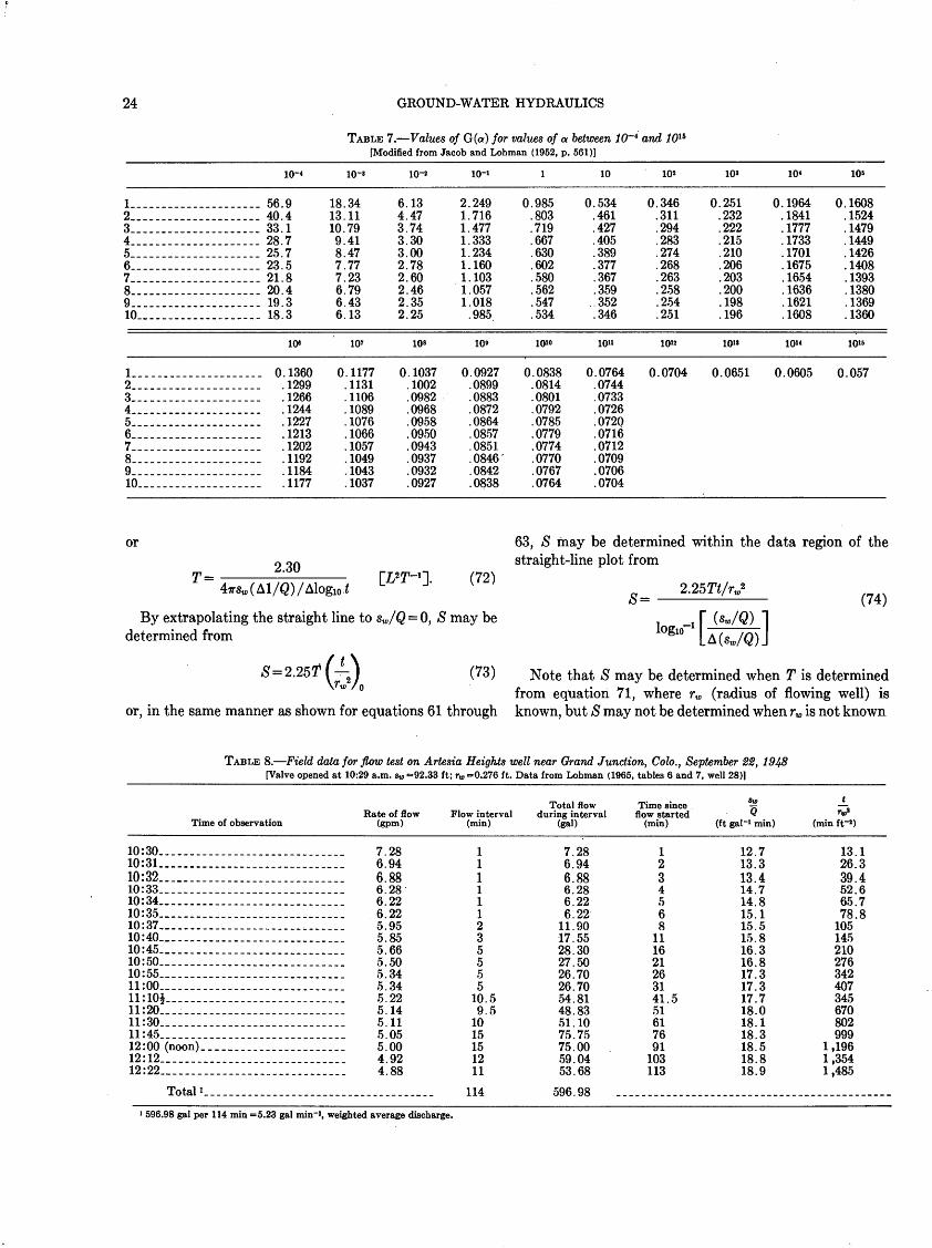
24 GROUND-WATER HYDRAULICS
TABLE 7. Values of G(a) for values of a between 10~* and 10U[Modified from Jacob and Lohman (1952, p. 561)]
1. _-_--_----.2... .........3............4............5............6............7............8-.....-..-..9...........10.--.....-..
1. ..--....-.23... .........45.. ._..._....6............78............9............10...........
.......... 56.
.......... 40.
.......... 33.
.......... 28.
.......... 25.
.......... 23.21
.......... 20.
.......--. 19.
.......... 18.
.......... 0
io-<
9417758433
10"
.1360
.1299
.1266,1244,1227.1213.1202.1192.1184.1177
io-»
18.3413.1110.799.418.477.777.236.796.436.13
10'
0.1177.1131.1106.1089.1076.1066.1057.1049.1043.1037
io-s
6.134.473.743.303.002.782.602.462.352.25
10«
0.1037.1002.0982.0968.0958.0950.0943.0937.0932.0927
iO-»
2.2491.7161.4771.3331.2341.1601.1031.0571.018.985
10»
0.0927.0899.0883.0872.0864.0857.0851.0846'.0842.0838
i
0.985.803.719.667.630.602.580.562.547.534
10"
0.0838.0814.0801.0792.0785.0779.0774.0770.0767.0764
10
0.534.461.427.405.389.377.367.359.352.346
10»
0.0764.0744.0733.0726.0720.0716.0712.0709.0706.0704
10'
0.346.311.294.283.274.268.263.258.254.251
10»
0.0704
108
0.251.232.222.215.210.206.203.200.198.196
10"
0.0651
10«
0.1964.1841.1777.1733.1701.1675. 1654.1636.1621.1608
10"
0.0605
10«
0.1608. 1524.1479.1449.1426.1408.1393.1380.1369.1360
10»5
0.057
or
2.30
4T«»(Al/Q)/AlogI0 .((72)
63, S may be determined within the data region of the straight-line plot from
0__2.25 Tt/rwz
By extrapolating the straight line to sw/Q = 0, S may be determined from
logirl r^/«Li(74)
(73) Note that S may be determined when T is determined from equation 71, where rw (radius of flowing well) is
or, in the same manner as shown for equations 61 through known, but S may not be determined when rw is not known
TABLE 8. Field data for flow test on Artesia Heights well near Grand Junction, Colo., September 22, 1948 [Valve opened at 10:29 a.m. tv, =92.33 ft; rw =0.276 ft. Data from Lohman (1965, tables 6 and 7, well 28)]
Time of observation
10:30...........................10:31...........................10:32...........................10:33.___._. ____________________10:34...........................10:35...........................10:37...........................10:40... ........................10:45...........................10:50..........................10:55..........................11:00..........................11:10$.... .._-..___.___._._____11:20..........................11:30... ...... .................ll:45._... ......................12:00 (noon)... _ _...__._.___..12:12........... ...............12:22._........... .............
Total 1 ...................
Rate of flow (gpm)
7.286.946.88
.... 6.286.226.225.955.85
.... 5.66
.... 5.505.345.34
.... 5.22
.... 5.145.11
.... 5.055.004.924.88
Flow interval (min)
111111235555
10.59.5
1015151211
114
Total flow during interval
(gal)
7.286.946.886.286.226.22
11.9017.5528.3027.5026.7026.7054.8148.8351.1075.7575.0059.0453.68
596.98
Time since flow started
(min)
1234568
111621263141.551617691
103113
Su,
Q (ft gal"1 min)
12.713.313.414.714.815.115.515.816.316.817.317.317.718.018.118.318.518.818.9
t V
(min ft~»)
13.126.339.452.665.778.8
105145210276342407345670802999
1,1961,3541,485
1 596.98 gal per 114 min =5.23 gal min'1, weighted average discharge.
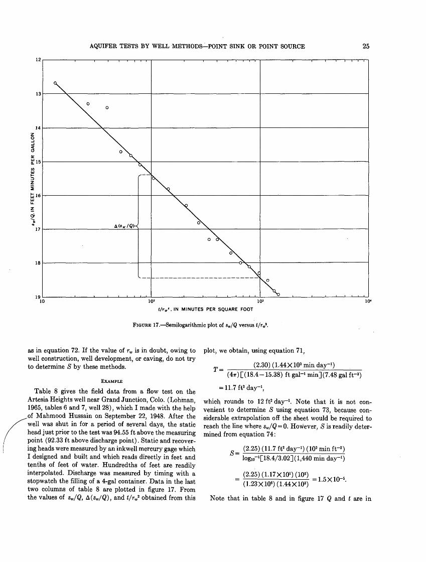
AQUIFER TESTS BY WELL METHODS POINT SINK OR POINT SOURCE 25
12
13 \
14
O
ccHJ IR Q. 15
16
zc*
17
18
1910 102 103
tAv'.IN MINUTES PER SQUARE FOOT
FIGURE 17. Semilogarithmic plot of sv/Q versus t/rtt*
as in equation 72. If the value of rw is in doubt, owing to well construction, well development, or caving, do not try to determine S by these methods.
EXAMPLE
Table 8 gives the field data from a flow test on the Artesia Heights well near Grand Junction, Colo. (Lohman, 1965, tables 6 and 7, well 28), which I made with the help
.of Mahmood Hussain on September 22, 1948. After the well was shut in for a period of several days, the static head just prior to the test was 94.55 ft above the measuring point (92.33 ft above discharge point). Static and recover ing heads were measured by an inkwell mercury gage which I designed and built and which reads directly in feet and tenths of feet of water. Hundredths of feet are readily interpolated. Discharge was measured by timing with a stopwatch the filling of a 4-gal container. Data in the last two columns of table 8 are plotted in figure 17. From the values of sw/Q, A (« ,/$), and t/rw2 obtained from this
plot, we obtain, using equation 71,
T = (2.30) (1.44Xl03 min day1 )(4ir) [(18.4-15.38) ft gal-1 min](7.48 gal fr3 )
= 11.7 ft2 day1 ,
which rounds to 12 ft2 day"1 . Note that it is not con venient to determine S using equation 73, because con siderable extrapolation off the sheet would be required to reach the line where sw/Q = 0. However, S is readily deter mined from equation 74:
Cf __ (2.25) (11.7 ft2 day1 ) (103 min fr2 ) loglo-1 [18.4/3.02](l,440 min day-1 )
(2.25)(1.17X101 )(103 ) = 1.5X10⁻⁵ .(1.23X10⁶)(1.44X10³ )
Note that in table 8 and in figure 17 Q and t are in
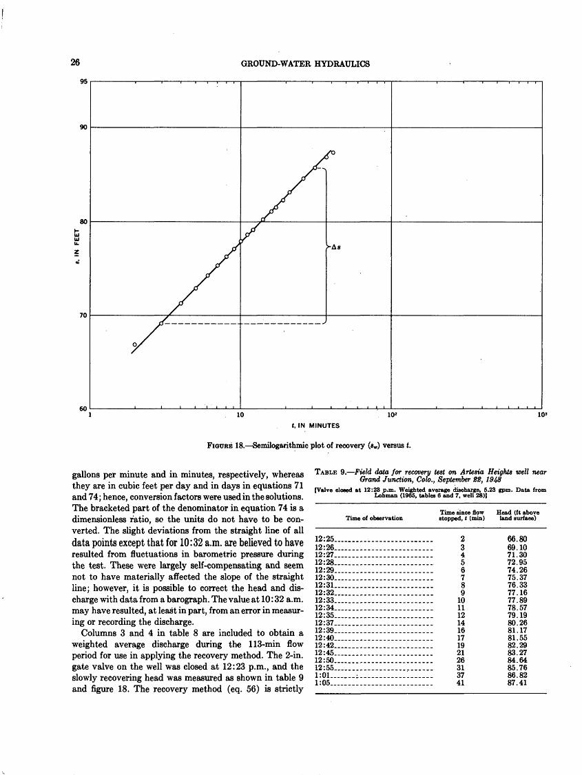
26 GROUND-WATER HYDRAULICS
60
t, IN MINUTES
FIGURE 18. Semilogarithmic plot of recovery (« ) versus t.
gallons per minute and in minutes, respectively, whereas they are in cubic feet per day and in days in equations 71 and 74; hence, conversion factors were used in the solutions. The bracketed part of the denominator in equation 74 is a dimensionless ratio, so the units do not have to be con verted. The slight deviations from the straight line of all data points except that for 10:32 a.m. are believed to haveresulted from fluctuations in barometric pressure during the test. These were largely self-compensating and seem not to have materially affected the slope of the straight line; however, it is possible to correct the head and dis charge with data from a barograph. The value at 10:32 a.m. may have resulted, at least in part, from an error in measur ing or recording the discharge.
Columns 3 and 4 in table 8 are included to obtain a weighted average discharge during the 113-min flow period for use in applying the recovery method. The 2-in. gate valve on the well was closed at 12:23 p.m., and the slowly recovering head was measured as shown in table 9 and figure 18. The recovery method (eq. 56) is strictly
TABLE 9. Field data for recovery test on Artesia Heights well near Grand Junction, Colo., September 28, 1948
[Valve closed at 12:23 p.m. Weighted average discharge, 5.23 gpm. Data from Lohman (1965, tables 6 and 7, well 28)]
Time of observation
12:25.......................12:26.......................12:27.......................12:28......................12:29....... ................12:30 __--------12:31. .. ................12:32.......................12:33.......................12:34 ....... _....... ...12:35 . ........... ......12:37.......................12:39 .... ................12:40........... ........ ....12:42.......................12:45.......................12:50....... .............. ..12:55... ... ........... ......l:01-._-___;_._ ..........1:05........ ................
Time since flow stopped, t (min)
23456789
101112141617192126313741
Head (ft above land surface)
66.8069.1071.3072.9574.2675.3776.3377.1677.8978.5779.1980.2681.1781.5582.2983.2784.6485.7686.8287.41
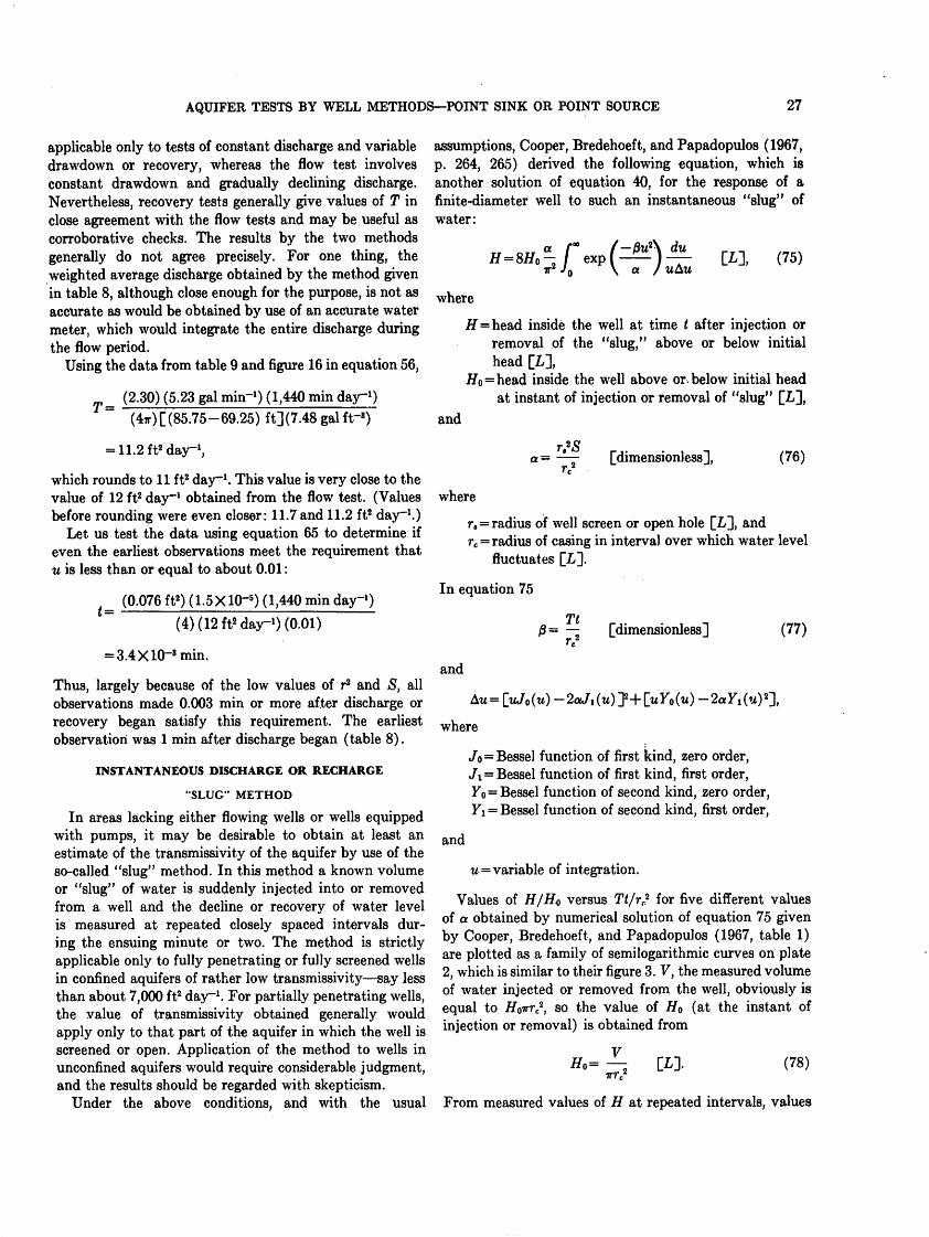
AQUIFER TESTS BY WELL METHODS POINT SINK OR POINT SOURCE 27
applicable only to tests of constant discharge and variable drawdown or recovery, whereas the flow test involves constant drawdown and gradually declining discharge. Nevertheless, recovery tests generally give values of T in close agreement with the flow tests and may be useful as corroborative checks. The results by the two methods generally do not agree precisely. For one thing, the weighted average discharge obtained by the method given in table 8, although close enough for the purpose, is not as accurate as would be obtained by use of an accurate water meter, which would integrate the entire discharge during the flow period.
Using the data from table 9 and figure 16 in equation 56,
T = (2.30) (5.23 gal min-1 ) (1,440 min day-1 ) (4») [(85.75-69.25) ft](7.48 gal fr8)
assumptions, Cooper, Bredehoeft, and Papadopulos (1967, p. 264, 265) derived the following equation, which is another solution of equation 40, for the response of a finite-diameter well to such an instantaneous "slug" of water:
= 11.2 ft2 day-1 ,
which rounds to 11 ft2 day-1 . This value is very close to the value of 12 ft2 day-1 obtained from the flow test. (Values before rounding were even closer: 11.7and 11.2 ft2 day"1 .)
Let us test the data using equation 65 to determine if even the earliest observations meet the requirement that u is less than or equal to about 0.01:
_ (0.076 ft2 ) (1.5X1Q-5 ) (1,440 min day-1 ) (4) (12 ft2 day-1 ) (0.01)
= 3.4X10⁻⁸ min.
Thus, largely because of the low values of r2 and S, all observations made 0.003 min or more after discharge or recovery began satisfy this requirement. The earliest observation was 1 min after discharge began (table 8).
INSTANTANEOUS DISCHARGE OR RECHARGE
"SLUG" METHOD
In areas lacking either flowing wells or wells equipped with pumps, it may be desirable to obtain at least an estimate of the transmissivity of the aquifer by use of the so-called "slug" method. In this method a known volume or "slug" of water is suddenly injected into or removed from a well and the decline or recovery of water level is measured at repeated closely spaced intervals dur ing the ensuing minute or two. The method is strictly applicable only to fully penetrating or fully screened wells in confined aquifers of rather low transmissivity say less than about 7,000 ft2 day"1 . For partially penetrating wells, the value of transmissivity obtained generally would apply only to that part of the aquifer in which the well is screened or open. Application of the method to wells in unconfined aquifers would require considerable judgment, and the results should be regarded with skepticism.
Under the above conditions, and with the usual
(75)
where
= head inside the well at time t after injection or removal of the "slug," above or below initial head [L],
o = head inside the well above or. below initial head at instant of injection or removal of "slug" [L],
and
[dimensionless], (76)
where
r, = radius of well screen or open hole [L], and rc = radius of casing in interval over which water level
fluctuates [L].
In equation 75
Tt /3= - [dimensionless] (77)
and
(w) -2aJl (u')J-}-luY0 (u) -
where
«/o = Bessel function of first kind, zero order, «/i = Bessel function of first kind, first order, y0 = Bessel function of second kind, zero order, YI = Bessel function of second kind, first order,
and
w= variable of integration.
Values of H/H0 versus Tt/rr* for five different values of a obtained by numerical solution of equation 75 given by Cooper, Bredehoeft, and Papadopulos (1967, table 1) are plotted as a family of semilogarithmic curves on plate 2, which is similar to their figure 3. V, the measured volume of water injected or removed from the well, obviously is equal to H0irrcz , so the value of H0 (at the instant of injection or removal) is obtained from
Ho= [L]. irr 2 (78)
From measured values of H at repeated intervals, values
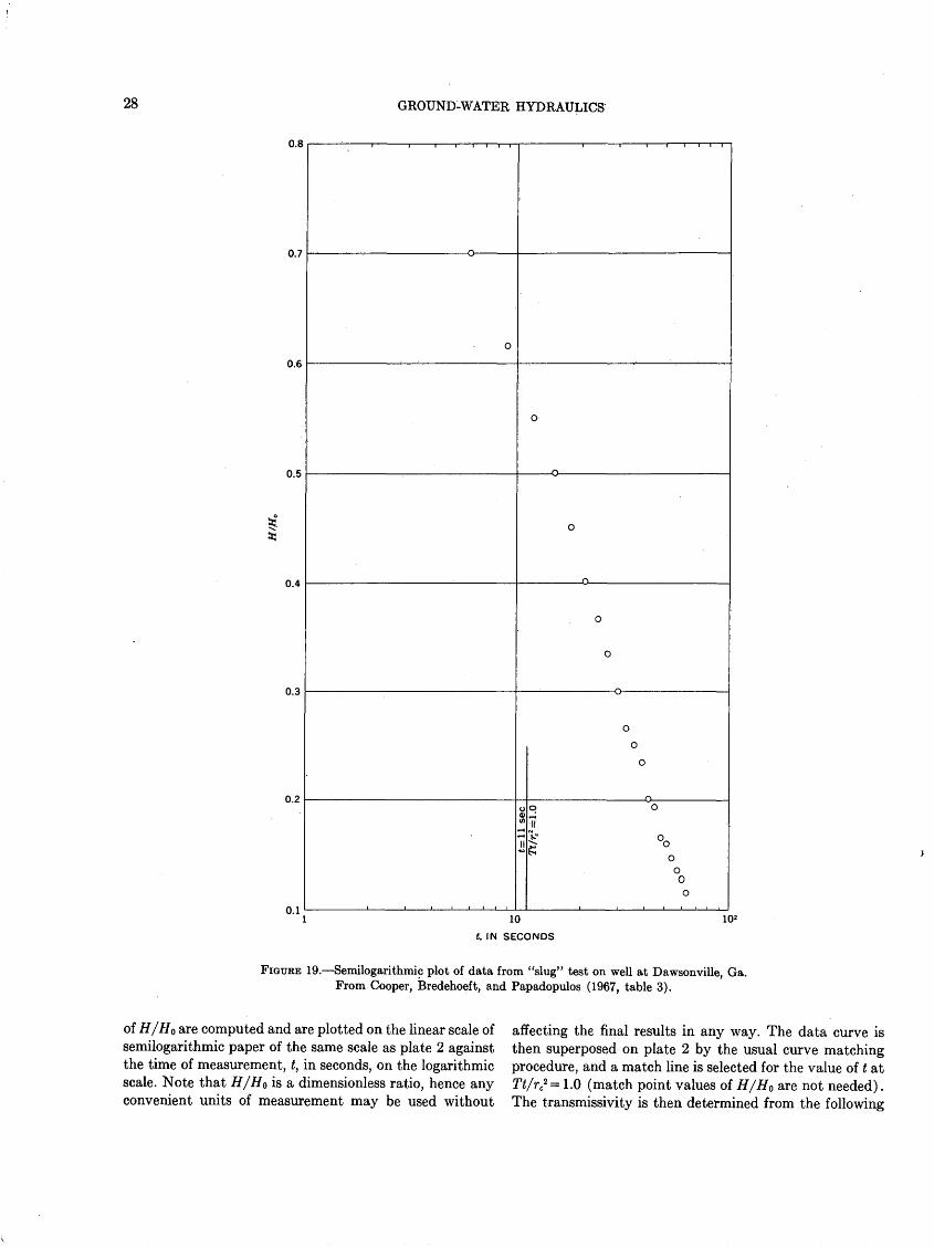
28 GROUND-WATER HYDRAULICS
0.8
0.7
0.6
0.5
0.4
0.3
0.2
0.110
t, IN SECONDS
102
FIGURE 19. Semilogarithmic plot of data from "slug" test on well at Dawsonville, Ga. From Cooper, Bredehoeft, and Papadopulos (1967, table 3).
of H/Ho are computed and are plotted on the linear scale of semilogarithmic paper of the same scale as plate 2 against the time of measurement, t, in seconds, on the logarithmic scale. Note that H/H0 is a dimensionless ratio, hence any convenient units of measurement may be used without
affecting the final results in any way. The data curve is then superposed on plate 2 by the usual curve matching procedure, and a match line is selected for the value of t at Tt/r*= 1.0 (match point values of H/H0 are not needed). The transmissivity is then determined from the following
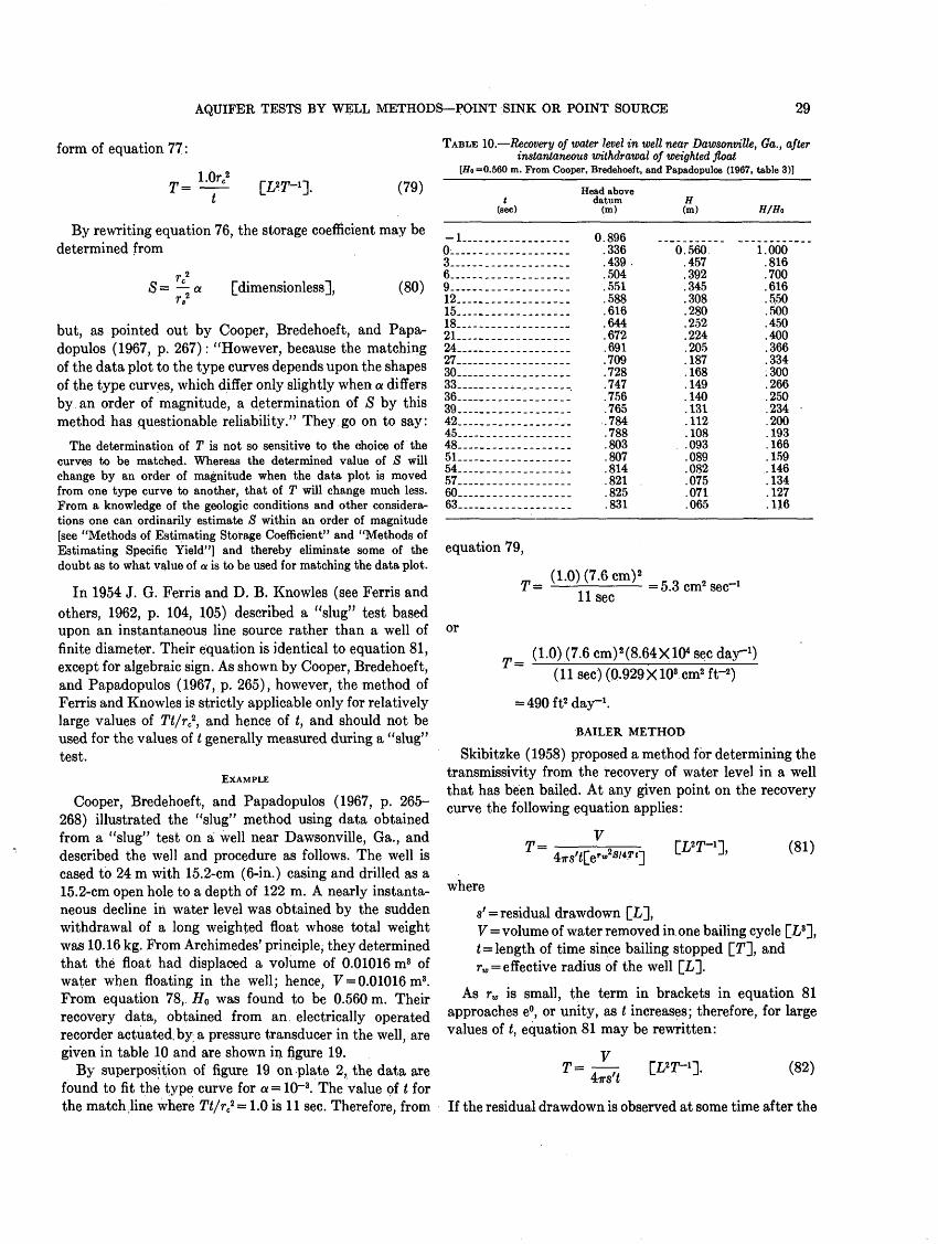
AQUIFER TESTS BY WELL METHODS POINT SINK OR POINT SOURCE 29
form of equation 77:
T= 1 OrI
TABLE 10. Recovery of water level in well war Dawsonville, Ga., after instantaneous withdrawal of weighted float
[Ho =0.560 m. From Cooper, Bredehoeft, and Papadopuloe (1967, table 3)]
(79)
By rewriting equation 76, the storage coefficient may be determined from
S = a [dimensionless], (80)
but, as pointed out by Cooper, Bredehoeft, and Papa dopulos (1967, p. 267): "However, because the matching of the data plot to the type curves depends upon the shapes of the type curves, which differ only slightly when a differs by an order of magnitude, a determination of S by this method has questionable reliability." They go on to say:
The determination of T is not so sensitive to the choice of the curves to be matched. Whereas the determined value of S will change by an order of magnitude when the data plot is moved from one type curve to another, that of T will change much less. From a knowledge of the geologic conditions and other considera tions one can ordinarily estimate S within an order of magnitude [see "Methods of Estimating Storage Coefficient" and "Methods of Estimating Specific Yield"] and thereby eliminate some of the equation 79, doubt as to what value of a is to be used for matching the data plot.
t(sec)
-1 ............0 . ..............3 ...-.-.-......6..................9 ...............12.................15.................18 .2124.... .............27 .-.--.......30.... .............33................36.. ...............39. ............42................45. .............48 ............51... .............54 ............57 .............60. . 63. ............
Head abovedatum
(m)
0.896.336.439 ..504.551.588.616.644.672.691.709.728.747.756.765.784.788.803.807.814.821.825.831
H(m)
0.560.457.392.345.308.280.252.224.205.187.168.149.140.131.112.108.093.089.082.075.071.065
H/Ho
1.000.816.700.616.550.500.450.400.366.334:300.266.250.234.200.193.166.159.146.134.127.116
In 1954 J. G. Ferris and D. B. Knowles (see Ferris and others, 1962, p. 104, 105) described a "slug" test based upon an instantaneous line source rather than a well of finite diameter. Their equation is identical to equation 81, except for algebraic sign. As shown by Cooper, Bredehoeft, and Papadopulos (1967, p. 265), however, the method of Ferris and Knowles is strictly applicable only for relatively large values of Tt/r?, and hence of t, and should not be used for the values of t generally measured during a "slug" test.
EXAMPLE
Cooper, Bredehoeft, and Papadopulos (1967, p. 265- 268) illustrated the "slug" method using data obtained from a "slug" test on a well near Dawsonville, Ga., and described the well and procedure as follows. The well is cased to 24 m with 15.2-cm (6-in.) casing and drilled as a 15.2-cm open hole to a depth of 122 m. A nearly instanta neous decline in water level was obtained by the sudden withdrawal of a long weighted float whose total weight was 10.16 kg. From Archimedes' principle, they determined that the float had displaced a volume of 0.01016 m3 of water when floating in the well; hence, V = 0.01016 m3 . From equation 78, H0 was found to be 0.560 m. Their recovery data, obtained from an electrically operated recorder actuated,by a pressure transducer in the well, are given in table 10 and are shown in figure 19.
By superposition of figure 19 on plate 2, the data are found to fit the type curve for a = 10~3 . The value of t for the match line where Tt/rc2 = 1.0 is 11 sec. Therefore, from
T _ (1.0) (7.6 cm) 2 _ 11 sec
5.3 ! sec'
or
T= LO) (7.6 cm) 2 (8.64X!04 sec day1 )(11 sec) (0.929X108 cm2 ft~2)
= 490 ft2 day-1 .
BAILER METHOD
Skibitzke (1958) proposed a method for determining the transmissivity from the recovery of water level in a well that has been bailed. At any given point on the recovery curve the following equation applies:
T =ir«,2S/47'f (81)
where
s' = residual drawdown [L~],V = volume of water removed in one bailing cycle [I/3], t = length of time since bailing stopped [T~], and rw = effective radius of the well \_L~\.
As rw is small, the term in brackets in equation 81 approaches e°, or unity, as t increases; therefore, for large values of t, equation 81 may be rewritten:
(82)
If the residual drawdown is observed at some time after the

30 GROUND-WATER HYDRAULICS
completion of n bailing cycles, the following equation applies:
i r^i Vs(83)
If approximately the same volume of water is bailed during each cycle, equation 83 becomes
Equation 84 is applied to single values of V and s' and the summation of the reciprocal of the elapsed time between the time each bailer was removed from the well and the time of observation of s'. If T is to be expressed in square feet per day, then obviously V should be expressed in cubic feet, s' in feet, and t in days, or suitable con versions of units should be made.
The bailer method should give satisfactory estimates of T for wells in confined aquifers having sufficiently shallow water levels to permit short time intervals between bailing cycles. In wells in unconfined aquifers, or in wells having relatively deep water levels, the method should be used with considerable judgment or not at all. (See also "Precautions.")
Unfortunately, I have no data available with which to illustrate the bailer method.
LEAKY CONFINED AQUIFERS WITH VERTICAL MOVEMENT
The flow equations for confined aquifers under conditions of both constant discharge and constant drawdown dis cussed in earlier sections of this report all are based upon the assumptions that the confining beds are impermeable (or have very low permeability), that they release no water from storage, and that vertical flow components are negligible. It is well known that no rocks are wholly impermeable and that some confining beds have finite permeability. We will now take up the equations for both steady and nonsteady radial flow from infinite aquiferswhose confining beds leak water either from or to the aquifer.
CONSTANT DISCHARGE
STEADY FLOW
Consider an aquifer overlain by a confining bed of low but finite permeability, which in turn is overlain by an unconfined aquifer. When discharge occurs from a well in a confined aquifer, the potentiometric surface is lowered throughout a large circular area (Cooper, 1963, p. 48). This lowering changes the relative head between the confined and unconfined aquifers and results in turn in a change in the rate of leakage through the confining bed.
The change may be either a decrease in the rate of leakage out of the aquifer or an increase in the rate of leakage into the aquifer, but either way the change results in a net increase in the supply of water to the aquifer and, there fore, constitutes capture of water.
Jacob (1946) derived an equation of steady flow near a well discharging at a constant rate from such an infinite leaky confined aquifer and described a graphical method for determining the transmissivity of the aquifer and the "leakance" of the confining bed. The leakance is the ratio K'/b', in which K' and V are the vertical hydraulic con ductivity and the thickness, respectively, of the confining beds. Hantush and Jacob (1954) derived equations for steady flow in variously bounded leaky confined aquifers. Later, equations for the more generally encountered non- steady flow in such aquifers were developed, and these will now be taken up.
NONSTEADY FLOW
HANTUSH- JACOB METHOD
Hantush and Jacob (1955) derived the following equation for nonsteady radial flow in an infinite leaky confined aquifer:
= 2K0 (2v)-
[dimensionless form], (85)where
and
= the modified Bessel function of the second kind of zero order,
= - V ~ [dimensionless], (86)
where
K' = the vertical hydraulic conductivity of the con fining bed [LT-1],
6'=the thickness of the confining bed [L], andT = the transmissivity of the aquifer [LZT~1 ~],
and
u = riS/^Tt [dimensionless], and y = the variable of integration.
The authors gave two series expressions for the formal solutions of equation 85 one for large values of t and one for small values and gave a few examples in both tabular and graphic form. In January 1956, Hilton H. Cooper, Jr., computed many values and prepared two families of type curves which were later published (Cooper, 1963, pi. 4). Meanwhile, unknown to Cooper, Hantush (1955) also had computed many values. (See also Hantush, 1956.)

AQUIFER TESTS BY WELL METHODS POINT SINK OR POINT SOURCE 31
TABLE 11. Postulated water-level drawdowns in three observation wells during a hypothetical test of an infinite leaky confined aquifer[Pumped well began discharging 1,000 gal min~> at <-0 min.) From Cooper (1963, p. 54)
Welll (r- 100 ft)
Time since pumping began, t
Min
0.2...........5...........1.... ........2............5..--.....-..10...........20--........50...........100..........200 - .500----.--.1,000 .....
Day
...... 0.000139
...... .000347
...... .000694
...... .00139
...... .00347
...... .00694
...... .0139
...... .0347
...... .0694
...... .139
...... .347
...... .694
tT*
(day ft-*)
1. 39X10-" 3. 47X10-" 6. 94X10-" 1.39X10⁻⁷ 3.47X10⁻⁷ 6.94X10⁻⁷ 1.39X10~« 3.47X10⁻⁹ 6.94X10~« 1.39X10-' 3.47X10-' 6.94X10-'
Drawdown, a (ft)
1.76 2.75 3.59 4.26 5.28 5.90 6.47 6.92 7.11 7.20 7.21 7.21
As described by Cooper (1963) , if the right-hand side of equation 85 is represented by L(u, v), the L, or leakance, function of u and v. eauation 85 mav be written
Well 2 (r -600 ft)
r* (day ft-*)
5.56X10⁻¹⁰ 1.39X10-' 2.78X10-' 5.56X10-' 1. 39X10-" 2. 78X10-" 5. 56X10-" 1.39X10⁻⁷ 2.78X10'7 5.56X10⁻⁷ 1.39X10-* 2.78X10-*
respectively,
r <!
Drawdown, « (ft)
0.01 .14 .45 .93
1.76 2.34 2.85 3.31 3.50 3.51 3.52 3.52
,000 gal min-1
Well 3 (r = 1,000 ft)
tfl Drawdown,
(day ft~«) (ft)
1.39X10⁻¹⁰ 3.47X10⁻¹⁰ 6.94X10-'° 1.39X10-' 3.47X10-' 6.94X10-' 1. 39X10-" 3. 47X10-" 6. 94X10-" 1.39X10⁻⁷ 3.47X10⁻⁷ 6.94X10⁻⁷
) (1,440 min day-1 ) (1
0.00 .00 .02 .14 .55 .99
1.46 1.95 2.10 2.11 2.11 2.11
.0)
[L].
S is determined by
t/r2S=4T [dimensionless]
l/u
(87)
(88)
(47r) (1.15 ft) (7.48 gal ft-3)
= 13,300 ft2 day-1 (rounded)and
and
K^b'
S(-
t(89)
= 10~4 (rounded) .
The plotted values for observation well 1 fall slightly below the solid-line curve for v = 0.02, or at about 0.025. Substituting r = 100ft, v = 0.025, and T= 13,300 ft2 day-1 in the first part of equation 89 gives
When K' and, hence, v approach zero, it can be shown that L(u, v) approaches W(u), and equation 87 becomes equation 46, the Theis equation. An enlargement of two families of type curves of L(u, v) versus l/u prepared by Cooper (1963, pi. 4) is shown on plate 3A. In one family of curves, v is the parameter; in the other, v2/u is the parameter. The solid-line type curves (v) correspond to a plot of s (vertical) versus t at some constant r, plotted as t/r2 (horizontal). The dashed-line curves (v*/u) correspond to a plot of s versus t/r2 at some constant t.
EXAMPLE
Table 11 from Cooper (1963, p. 54) gives postulated drawdowns in observation wells at distances of 100, 500, and 1,000 ft from a well discharging at the constant rate of 1,000 gpm for 1,000 min from a leaky confined aquifer. Values of s versus t/r2 for the three wells are shown on plate 35 superposed on the type curves. Note that a match point was chosen where a(u, v) = 1.0, l/w= 1.0, s = 1.15 ft, and 0* = 1.87X10"* day ft~2 . Substituting appropriate values in equations 87 (solved for T) and 88 gives,
K'-- = (4) (13,300 ft2 day1 ) =0.0033 day-1 .
Assume &' = 100 ft, then tf' = 0.33 ft day"1 .As the data in table 11 represent idealized conditions,
the same values for K'/b' would be obtained using the data for observation wells 2 and 3. Also, the same values of K'/b' would be obtained using the dashed-line curves by plotting the values of s for each observation well for some constant t, say 100 min (0.0694 day) , and substituting the value of v2/u, s, and t in the second part of equation 89.
Cooper (1963, p. 55) gives the following pertinent con clusions in regard to this method :
Because the adjustment of the hydraulic gradient through a confining bed generally lags considerably behind the decline in head, the water yielded by an artesian aquifer is derived largely, if not entirely, from storage in the confining bed. For this reason, most time-drawdown plots deviate from the Theis curve to a greater degree than if leakage alone were involved. The method for deter mining leakance is presented with reservation because, if applied under the mistaken assumption that the deviations are due to leakage, it yields erroneously large values. However, whenever the results of an aquifer test indicate that leakage occurs, the deter-
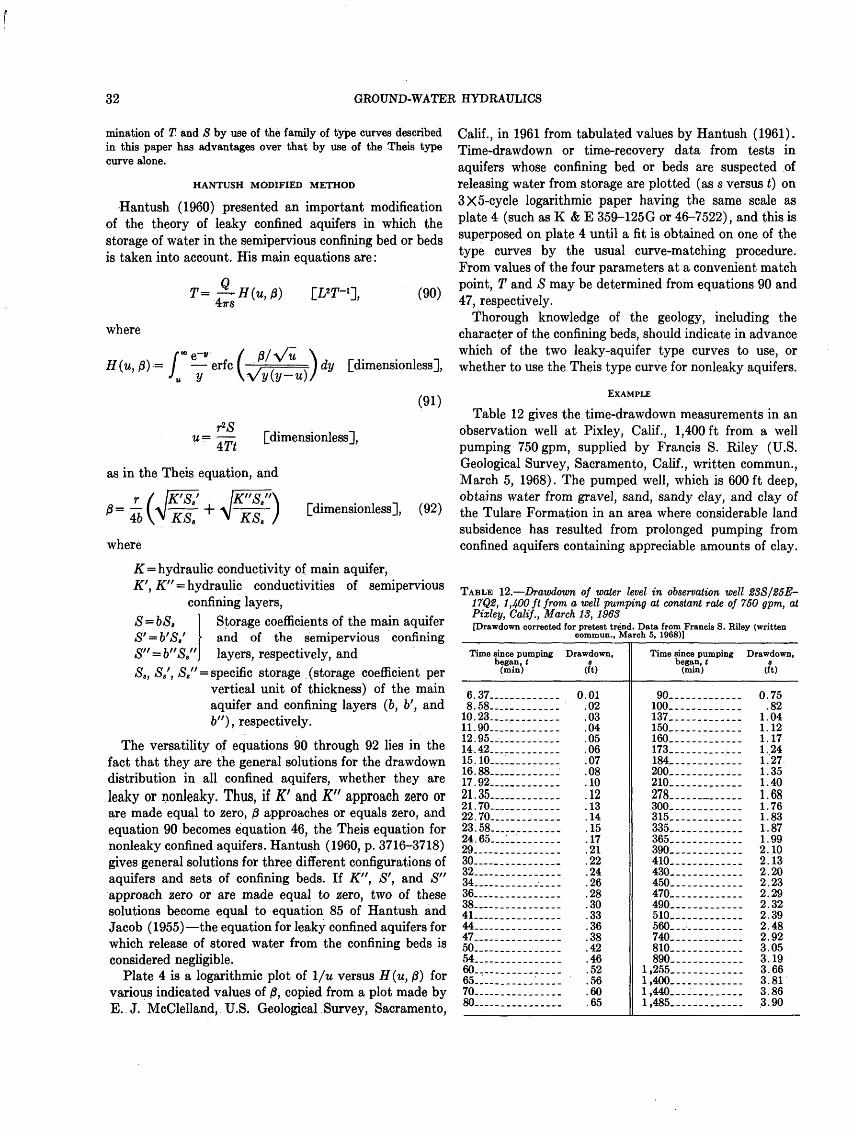
32 GROUND-WATER HYDRAULICS
mination of T and S by use of the family of type curves described in this paper has advantages over that by use of the Theis type curve alone.
HANTUSH MODIFIED METHOD
Hantush (1960) presented an important modification of the theory of leaky confined aquifers in which the storage of water in the semipervious confining bed or beds is taken into account. His main equations are:
(90)
where
/" &~v / 8/\/u \ erfc I , , == J dy [dimensionless],
« y \Vy(y-u)/
(91)
u= [dimensionless],
as in the Theis equation, and
r / /#"' Q ' IK" Sf "\'8= 46 \ v~Kff~ + V~KS~) Hdimensionless} (92)
where
K = hydraulic conductivity of main aquifer, K', K" = hydraulic conductivities of semipervious
confining layers,Storage coefficients of the main aquifer and of the semipervious confining layers, respectively, and
S,, S8 f, S3" = specific storage .(storage coefficient per vertical unit of thickness) of the main aquifer and confining layers (6, &', and 6"), respectively.
The versatility of equations 90 through 92 lies in the fact that they are the general solutions for the drawdown distribution in all confined aquifers, whether they are leaky or nonleaky. Thus, if K' and K" approach zero or are made equal to zero, /3 approaches or equals zero, and equation 90 becomes equation 46, the Theis equation for nonleaky confined aquifers. Hantush (1960, p. 3716-3718) gives general solutions for three different configurations of aquifers and sets of confining beds. If K", S', and S" approach zero or are made equal to zero, two of these solutions become equal to equation 85 of Hantush and Jacob (1955) the equation for leaky confined aquifers for which release of stored water from the confining beds is considered negligible.
Plate 4 is a logarithmic plot of l/u versus H(u, /3) for various indicated values of /3, copied from a plot made by E. J. McClelland, U.S. Geological Survey, Sacramento,
Calif., in 1961 from tabulated values by Hantush (1961). Time-drawdown or time-recovery data from tests in aquifers whose confining bed or beds are suspected of releasing water from storage are plotted (as s versus t) on 3X5-cycle logarithmic paper having the same scale as plate 4 (such as K & E 359-125G or 46-7522), and this is superposed on plate 4 until a fit is obtained on one of the type curves by the usual curve-matching procedure. From values of the four parameters at a convenient match point, T and S may be determined from equations 90 and 47, respectively.
Thorough knowledge of the geology, including the character of the confining beds, should indicate in advance which of the two leaky-aquifer type curves to use, or whether to use the Theis type curve for nonleaky aquifers.
EXAMPLE
Table 12 gives the time-drawdown measurements in an observation well at Pixley, Calif., 1,400 ft from a well pumping 750 gpm, supplied by Francis S. Riley (U.S. Geological Survey, Sacramento, Calif., written commun., March 5, 1968). The pumped well, which is 600 ft deep, obtains water from gravel, sand, sandy clay, and clay of the Tulare Formation in an area where considerable land subsidence has resulted from prolonged pumping from confined aquifers containing appreciable amounts of clay.
TABLE 12. Drawdown of water level in observation well 23S/25E- 17Q%, 1,400 ft from a well pumping at constant rate of 760 gpm, at Pixley, Calif., March IS, 1968[Drawdown corrected for pretest trend. Data from Francis S. Riley (written
commun., March 5, 1968)]
Time since pumping began, t
(min)
6. 37.. ___________8. 58... ._........
10. 23.. .._........11. 90...._. .......12. 95.... _........14. 42.. .._........15.10.............16. 88.. ...........17. 92.. .__...__...21.35.............21.70.............22. 70.. ...........23.58.............24.65.............29... .............30...............32................34................36................38... .............41................44... .............47 ____________50... .............54... .............60...............65....... ________70... .............80 ____________
Drawdown,
(ft)
0.01.02.03.04.05.06.07.08.10.12.1314
.15
.17212224
.26
.28
.30
.33
.36
.3842
.46
.52
.56
.60
.65
Time since pumping began, t
(min)
90.............100_. -_..____._.137.............ISO.............160.............173.............184.............200.............210....._.......278...... ......300..-.-.-......315,. ._______._.335.............365.............390.............410.... .........430............450..-.-.-.....470............490............510............560............740............810............890............
1,255............1,400.... ...... ..1,440..---.......1,485.. ..........
Drawdown,
(ft)
0.75.82
1.041 121.171.241.271.351.401.681.761.83
. 1.87
. 1.99
. 2.10
. 2.13
. 2.20
. 2.23
. 2.29
. 2.32
. 2.39
. 2.48
. 2.92
. 3.05
. 3.19
. 3.66
. 3.81
. 3.86
. 3.90
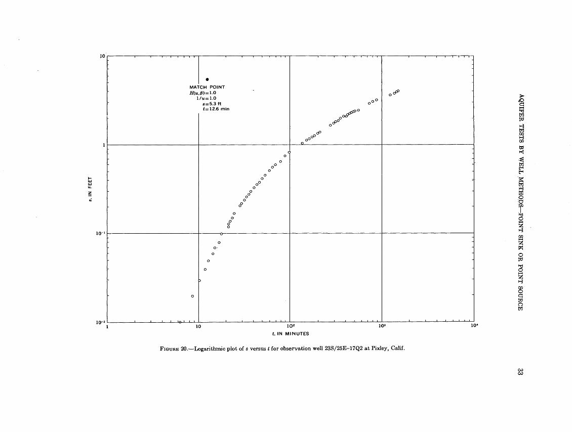
AQ
UIFE
R T
EST
S BY
WE
LL
ME
TH
OD
S P
OIN
T SIN
K O
R PO
INT
SOU
RC
E33
o o
\
O o
q m
^Q. ^J ^
in ^T
II
II II
IIr; c
s °° ** o
<o. <!
-1 2
" O03 (N<y03
13
3d
N
l '»

34 GROUND-WATER HYDRAULICS
(See table 3, "Tulare-Wasco area.") The aquifer is con- wherefined by the Corcoran Clay Member, about 6ft thick, above which is an unconfined aquifer about 200 ft thick. A logarithmic plot of s versus t from table 12 is shown in figure 20, which shows also the match-point values of the four parameters obtained by superposition on plate 4. From these data, T and S are computed from equations 90 and 47, as follows:
_ (750 gal min-1 ) (1,440 min day-1 ) (1.0) (47r) (5.3 ft) (7.48 gal fr3)
= 2, 170 ft2 day-1 ,
rounded to 2,200 ft2 day-1 , and
4Ttu (4) (2,170 ft2 day-1 ) (12.6 min)S=r2 (1,400 ft) 2 (l,440 min day-1 ) (1/1.0)
= 3.9X10⁻⁵,
rounded to 4 X10~5.Preliminary attempts to fit both early and late data from
table 12, and similar drawdown and recovery data from two other observation wells at r = 650 and 1,220 ft, to the Theis curve gave apparent values of T from 5 to 20 times the more realistic value computed above, and apparent values of S from 17 to 25 times the value computed above.
CONSTANT DRAWDOWN
Hantush (1959) derived an equation for determining T and S for a well of constant drawdown that is discharging by natural flow from an infinite leaky confined aquifer, and he also gave solutions for a circular leaky confined aquifer with zero drawdown on the outer boundary and for a closed circular aquifer. The equations for the infinite leaky confined aquifer follow:
Q2irswG(a, rw/B)
where
Tt[dimensionless],
[L2],
(93)
(94)
(95)and
wexp( cm2 ) du[dimensionless],
Ki = Modified Bessel function of second kind, firstorder,
KQ= Modified Bessel function of second kind, zeroorder,
Jo= Bessel function of first kind, zero order, F0 =Bessel function of second kind, zero order, and u variable of integration.
The integral in equation 96 cannot be integrated directly but was evaluated numerically, and values of the param eters are given by Hantush (1959, table 1) from which plate 5 was drawn after Walton (1962, pi. 4). When £=«>, r»/B and K'b' (equal to T/B2)=0, so that the parent-type curve on plate 5 is the same as on plate 1 the nonleaky-type curve of Jacob and Lohman (1952, fig. 5) except, of course, that the values of the parameters differ.
On translucent logarithmic paper of the same scale as plate 5 (such as Codex 4123) values of Q are plotted on the vertical scale against values of t on the horizontal scale, and the data curve is superposed on plate 5. From the match point obtained by the usual curve matching procedure, preferably at G(a, rw/B) and a = 1.0, values of the four parameters G(a, rw/B), a, Q, and t are obtained. T is then determined using equation 93, and S is deter mined by rewriting equation 94:
S= Tt[dimensionless]. (97)
Unfortunately, I have no field .data with which to illustrate this method.
UNCONFINED AQUIFERS WITH VERTICAL MOVEMENT
Boulton (1954a) derived an integral equation for the drawdown of the water table near a discharging well before the flow approaches steady state, which is founded partly on a consideration of vertical flow components, such as those that prevail near the well during the early stages of a pumping test in an unconfined aquifer. (See Stallman, 1961a.) In our notation, his partial differential equation describing the head (h) at the water table is
5 fAs equation 98 is nonlinear and cannot readily be solved, he assumes that the head gradients are small enough that their squares may be neglected, whence
dh Kdh dt S dz~
(99)
(96) where h = pressure head (p/gp) plus elevation head (z).
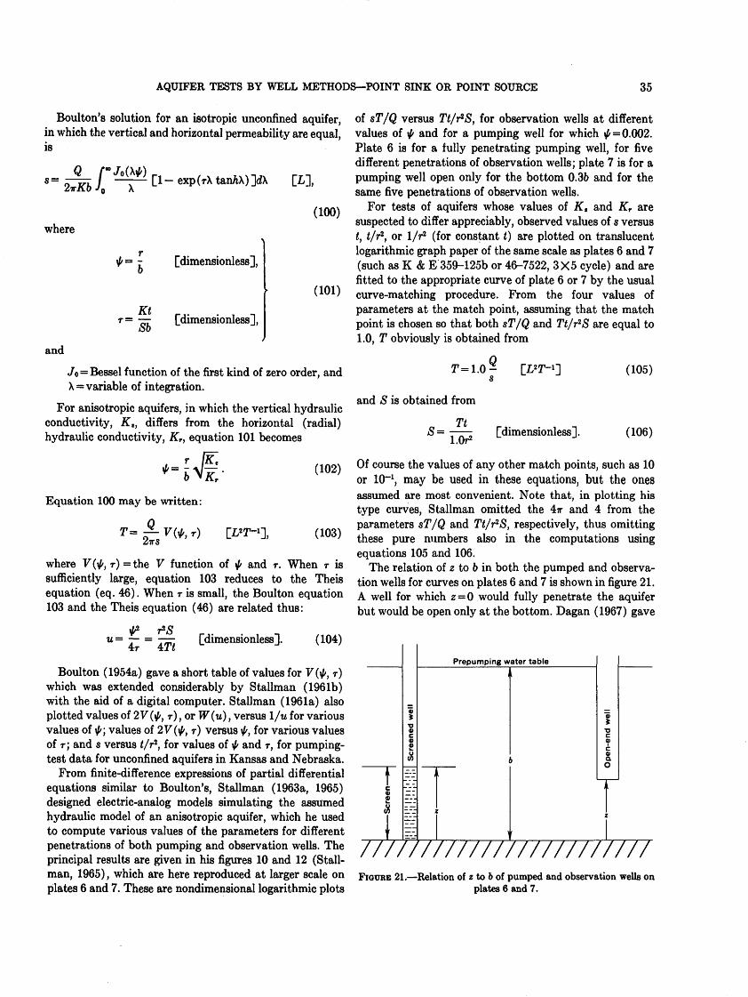
AQUIFER TESTS BY WELL METHODS POINT SINK OR POINT SOURCE 35
Boulton's solution for an isotropic unconfined aquifer, in which the vertical and horizontal permeability are equal, is
Q[1 - exp (rX tan/iX) ]dX [L],
(100)where
[dimensionless],
KtT= [dimensionless],
oo
(101)
and
Jo = Bessel function of the first kind of zero order, and X = variable of integration.
For anisotropic aquifers, in which the vertical hydraulic conductivity, Kt, differs from the horizontal (radial) hydraulic conductivity, Kr, equation 101 becomes
(102)
(103)
where V(\l/, T) =the V function of ^ and T. When r is sufficiently large, equation 103 reduces to the Theis equation (eq. 46). When T is small, the Boulton equation 103 and the Theis equation (46) are related thus:
*=r\h^
Equation 100 may be written:
= = U ~ 4r " [dimensionless]. (104)
Boulton (1954a) gave a short table of values for V(ift, T) which was extended considerably by Stallman (1961b) with the aid of a digital computer. Stallman (1961a) also plotted values of 2V(if/, T) , or W(u) , versus 1/u for various values of ^; values of 2V (^, T) versus \l/, for various values of T; and s versus t/r2 , for values of ^ and T, for pumping- test data for unconfined aquifers in Kansas and Nebraska.
From finite-difference expressions of partial differential equations similar to Boulton's, Stallman (1963a, 1965) designed electric-analog models simulating the assumed hydraulic model of an anisotropic aquifer, which he used to compute various values of the parameters for different penetrations of both pumping and observation wells. The principal results are given in his figures 10 and 12 (Stall man, 1965), which are here reproduced at larger scale on plates 6 and 7. These are nondimensional logarithmic plots
of sT/Q versus Tt/r*S, for observation wells at different values of $ and for a pumping well for which ^ = 0.002. Plate 6 is for a fully penetrating pumping well, for five different penetrations of observation wells; plate 7 is for a pumping well open only for the bottom 0.36 and for the same five penetrations of observation wells.
For tests of aquifers whose values of Kt and Kr are suspected to differ appreciably, observed values of s versus t, t/r2 , or 1/r2 (for constant t) are plotted on translucent logarithmic graph paper of the same scale as plates 6 and 7 (such as K & E 359-125b or 46-7522, 3X5 cycle) and are fitted to the appropriate curve of plate 6 or 7 by the usual curve-matching procedure. From the four values of parameters at the match point, assuming that the match point is chosen so that both sT/Q and Tt/r2S are equal to 1.0, T obviously is obtained from
T=1.0-s
and S is obtained from
TtS =l.Or2
[dimensionless].
(105)
(106)
Of course the values of any other match points, such as 10 or 10~l, may be used in these equations, but the ones assumed are most convenient. Note that, in plotting his type curves, Stallman omitted the 4ir and 4 from the parameters sT/Q and Tt/r2S, respectively, thus omitting these pure numbers also in the computations using equations 105 and 106.
The relation of z to 6 in both the pumped and observa tion wells for curves on plates 6 and 7 is shown in figure 21. A well for which z = 0 would fully penetrate the aquifer but would be open only at the bottom. Dagan (1967) gave
Prepumping water table
FIGURE 21. Relation of 2 to 6 of pumped and observation wells on plates 6 and 7.
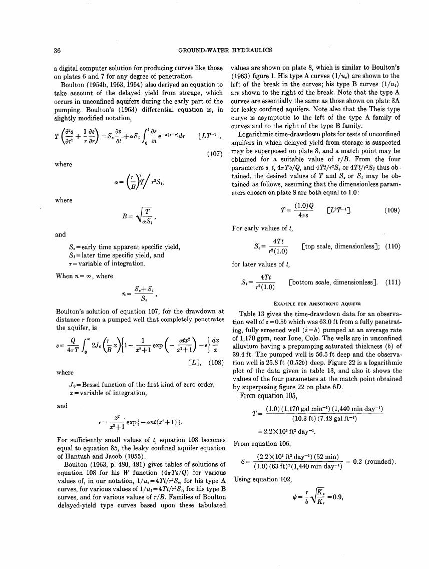
36 GROUND-WATER HYDRAULICS
a digital computer solution for producing curves like those on plates 6 and 7 for any degree of penetration.
Boulton (1954b, 1963, 1964) also derived an equation to take account of the delayed yield from storage, which occurs in unconfined aquifers during the early part of the pumping. Boulton's (1963) differential equation is, in slightly modified notation,
1-*)- Se d̂ aSl C ̂ ,- rdr dt J dtdr* rdr/ dt
(107)
where
where
r'S,,
TB=\l-^,
and
Se = early time apparent specific yield, Si = later time specific yield, and T = variable of integration.
When n = <x> , where
n = Se +Si Se
Boulton's solution of equation 107, for the drawdown at distance r from a pumped well that completely penetrates the aquifer, is
o - -
where
ate? \ \ dxX2 +1/ J x
[L], (108)
Jo = Bessel function of the first kind of zero order, x = variable of integration,
and
exp{-cm<(z2 +l)}.
For sufficiently small values of t, equation 108 becomes equal to equation 85, the leaky confined aquifer equation of Hantush and Jacob (1955).
Boulton (1963, p. 480, 481) gives tables of solutions of equation 108 for his W function (4irTs/Q) for various values of, in our notation, l/ue = 4iTt/r2Se , for his type A curves, for various values of l/ui = 4Tt/r2Si, for his type B curves, and for various values of r/B. Families of Boulton delayed-yield type curves based upon these tabulated
values are shown on plate 8, which is similar to Boulton's (1963) figure 1. His type A curves (l/ue ) are shown to the left of the break in the curves; his type B curves (l/wj) are shown to the right of the break. Note that the type A curves are essentially the same as those shown on plate 3A for leaky confined aquifers. Note also that the Theis type curve is asymptotic to the left of the type A family of curves and to the right of the type B family.
Logarithmic time-drawdown plots for tests of unconfined aquifers in which delayed yield from storage is suspected may be superposed on plate 8, and a match point may be obtained for a suitable value of r/B. From the four parameters s, t, IvTs/Q, and 4Tt/r*Se or 4Tt/r2S t thus ob tained, the desired values of T and Se or Si may be ob tained as follows, assuming that the dimensionless param eters chosen on plate 8 are both equal to 1.0:
(1.0)347T5
(109)
For early values of t,
e_e r'(l.O)
for later values of t,
[top scale, dimensionless]; (110)
r2 (1.0)[bottom scale, dimensionless]. (Ill)
EXAMPLE FOR ANISOTROPIC AQUIFER
Table 13 gives the time-drawdown data for an observa tion well of z = 0.5& which was 63.0 ft from a fully penetrat ing, fully screened well (2 = 6) pumped at an average rate of 1,170 gpm, near lone, Colo. The wells are in unconfined alluvium having a prepumping saturated thickness (6) of 39.4 ft. The pumped well is 56.5 ft deep and the observa tion well is 25.8 ft (0.526) deep. Figure 22 is a logarithmic plot of the data given in table 13, and also it shows the values of the four parameters at the match point obtained by superposing figure 22 on plate 6Z).
From equation 105,
T = (1.0) (1,170 gal min-1 ) (1,440 min day-1 ) (10.3 ft) (7.48 gal ft-3 )
= 2.2X104 ft2 day~1 .
From equation 106,
Cf __(2.2X104 ft2 day-1 ) (52 min)
(1.0) (63 ft) 2 (l,440 min day-1 )
Using equation 102,
= 0.2 (rounded).
VI'=r\/^=o.9,
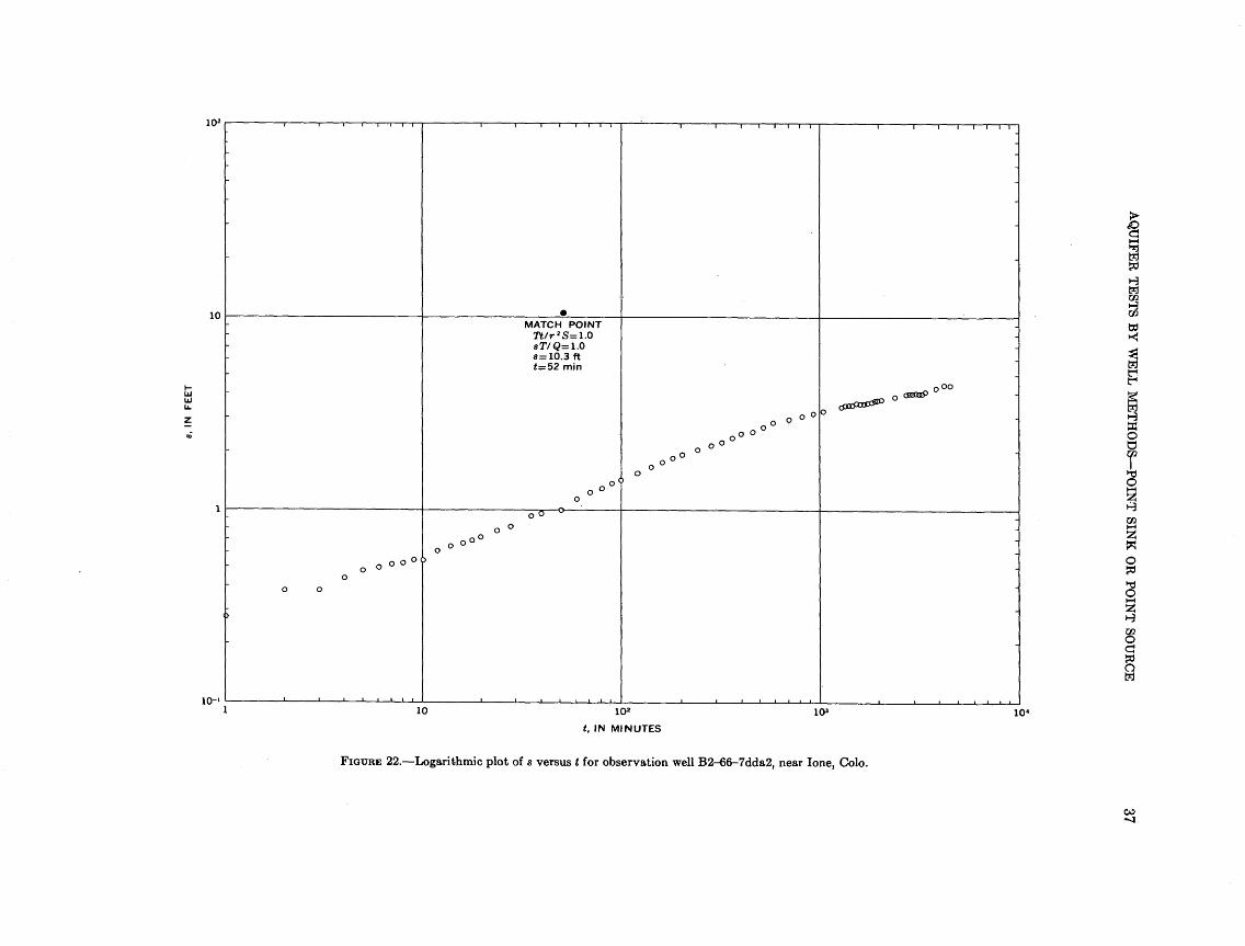
AQ
UIFE
R T
EST
S BY
WE
LL
ME
TH
OD
S P
OIN
T SIN
K O
R PO
INT
SOU
RC
E37
o o o
o o o
29
o o
I ~
QfO
pqO
£
^~
<in
fce^ II II<
H
w oo -w
oO O
O O
O O
O-
S
PQ1
oas UO
133d
N
l 's
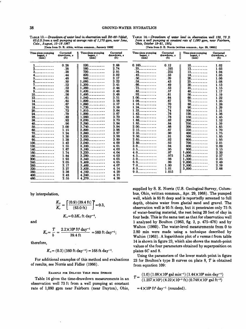
38 GROUND-WATER HYDRAULICS
TABLE 13. Drawdown of water level in observation well B2-66-7ddaS, 63.0 ft from a well pumping at average rate of 1,170 gpm, near lone, Colo., August, 15-18 1967
[Data from D. R. Albin, written eommun., January 1968]
Time since pumping began. t
(min)
I .......
3............4............5............6... .........7..... .......8.. ...9 ... 10 .......12............14..... .......16 18 . .20 24............28 36............40 50 60 70. ...80 90 -.--.-..
100 --.-....120 .......140 ----...160 .........180 .........200240. --------280 320 360 --------400-.. ...460...... ......
Corrected 1 drawdown, «
(ft) 1
0.28.38.38.44.48.50.52.53.56.56.61.65.67.70.72.79.82.92.96
1.001.151.241.301.381.421.551.671.741.841.932.052.172.272.362.482.55
Time since pumping began.*
(min)
520 580 .700 820..........940... ...... .
1,060.... ......1,300. 1,360. 1,420... 1,480 . 1, 540... .......1,600... .......1,660 1,720....... . ..1,810 1,900...-..--1,960 2,020 2,380..... -2,740.. ....... .2,800..........2,860..........2,920.....- 2,980 .. 3,040.-.--..--3,100. .-3,160..........3,220.... .3,280.........3,340. 3,400... ...... .3,460... ...... .3,820... .......4,180--.-.--.4,240. 4,270-.-.----.
Corrected drawdown, «
(ft)
2.662.742.913.023.173.223.413.443.483.483.513.563.573.593.643.673.703.733.843.943.963.973.983.994.004.014.024.044.034.054.054.074.144.204.214.20
by interpolation,
K. KT
I" (0.9) (39.4 ft)T L (63.0ft) J
= O.J
and
v Kr~b~2.2Xl04 ft2 day-1
39.4 ft= 560 ft day-1
therefore,
Kt = (0.3) (560 ft day-1 ) = 168 ft day-1 .
For additional examples of this method and evaluations of results, see Norris and Fidler (1966).
EXAMPLE FOR DELAYED YIELD FROM STORAGE
Table 14 gives the time-drawdown measurements in an observation well 73 ft from a well pumping at constant rate of 1,080 gpm near Fairborn (near Dayton), Ohio,
TABLE 14. Drawdown of water level in observation well 139, 73 ft from a well pumping at constant rate of 1,080 gpm, near Fairborn, Ohio, October 19-21, 1954
[Data from S. E. Morris (written eommun., Apr. 29, 1968)]
Time since pumping began, t
(mm)
0.165...........25............34............42............ 50.. ..........58 .66............75............83............92...........
1.00--....-....1.08...........1.16...........1.24...........1.33...........1.42...........1.50...........1.68.-...--....1.85...........2. 00 ........2.15...........2.35... ........2.50 2.65...........2.80 ........3.0............3.5............4.0............4.5............5.0............6.0..... .......7.0............8.0..... .......9.0............
Corrected 1 drawdown, a 1
(ft) 1
0.12.195.255.33.39.43.49.53.57.61.64.67.70.72.74.76.78.82.84.86.87.90.91.92.93.94.95.97.975.98.99
1.001.011.015
I Time since pumping began, t
(min)
10... -12......--..15..........18..........20..........25..........30.. ........35..........40..........50-.-.--....6070..........80.---......90..........
100..........120..........150..........J200 ... ....250..........300..........350..--.-....400.........500 . 600..........700..........800...-.-....900..........
1,000..........1,200..........1,500..........2,000..----....2,500. ---3,000 .
Corrected drawdown, «
(ft)
1.021.031 041.051.061 OS1.131.151.171 1Q1.221.251.281.291.311.361.451.521.591.65i:701.751.851.952.012.093.152.202.272.352.492.592.66
supplied by S. E. Norris (U.S. Geological Survey, Colum bus, Ohio, written eommun., Apr. 29, 1968). The pumped well, which is 85 ft deep and is reportedly screened to full depth, obtains water from glacial sand and gravel. The observation well is 95 ft deep, but it penetrates only 75 ft of water-bearing material, the rest being 20 feet of clay in four beds. This is the same test as that for observation well 1 analyzed by Boulton (1963, fig. 2, p. 475-476) and by Walton (1960). The water-level measurements from 0 to 2.80 min were made using a technique described by Walton (1963). A logarithmic plot of s versus t from table 14 is shown in figure 23, which also shows the match-point values of the four parameters obtained by superposition on plates 6C and 8.
Using the parameters of the lower match point in figure 23 for Boulton's type B curves on plate 8, T is obtained from equation 109:
T =(1.0) (1.08X10³ gal min-1 ) (1.44X10⁸ min day-1 )(1.257X101 ) (4.22X10⁻¹ ft) (0.748X101 gal ft~3 )
= 4 X104 ft2 day-1 (rounded).
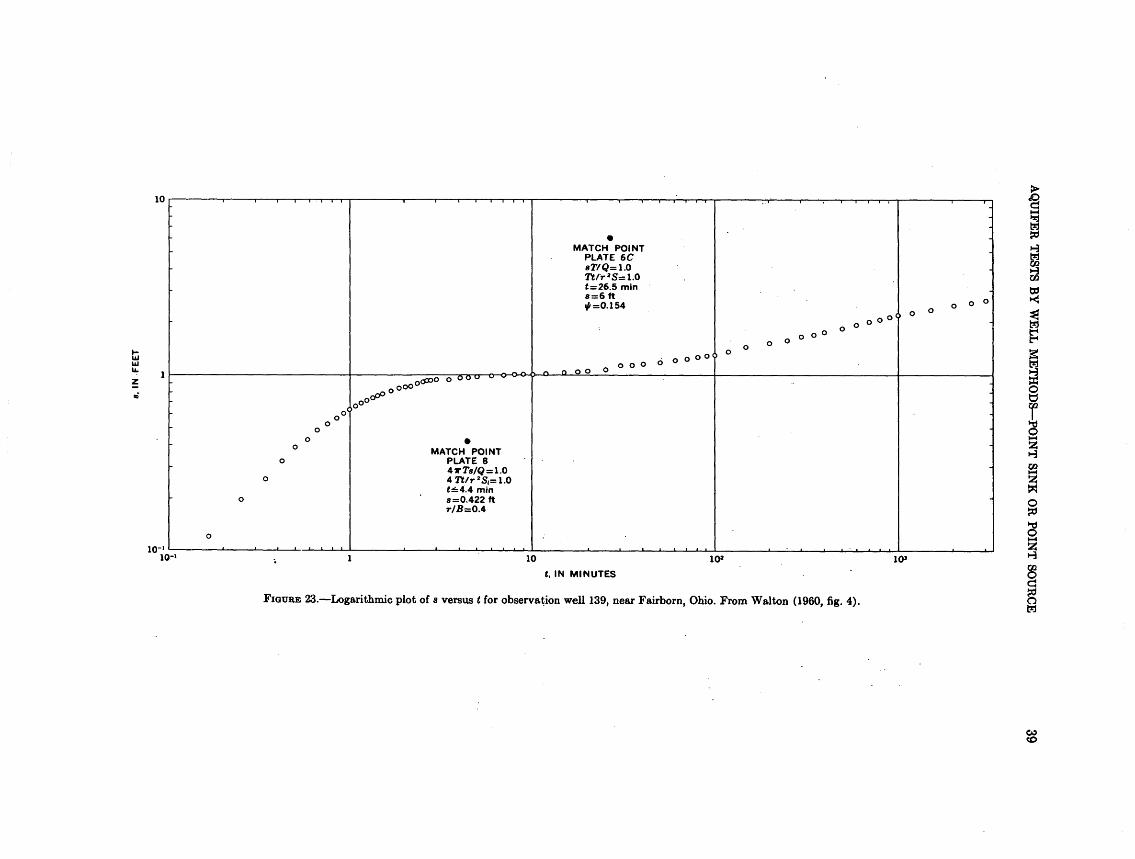
AQ
UIFER
TESTS BY
WELL M
ET
HO
DS PO
INT
SINK
OR
POIN
T SO
UR
CE
39
o o o o oo o o
Z.
9c
v
j o +
c
oo o o
K ~r
«»
JL<
o o oo8o o
o°0
oig~I2 Io oT21a ,o' *»
Oj
f?saI
133d
Nl '
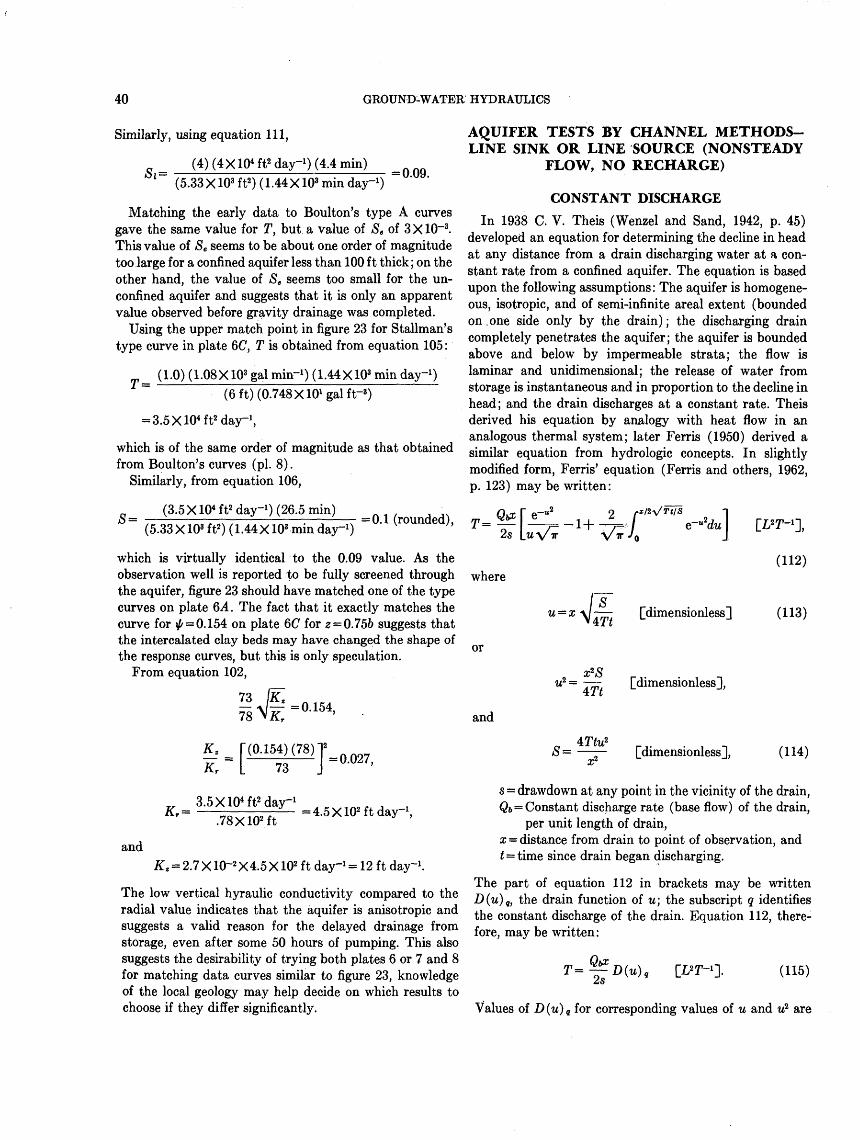
40 GROUND-WATER HYDRAULICS
Similarly, using equation 111,
(4) (4X104 ft2 day-1 ) (4.4 min) (5.33 X103 ft2 ) (1.44X10³ min day-1 )
= 0.09.
Matching the early data to Boulton's type A curves gave the same value for T, but a value of Se of 3X10~3. This value of Se seems to be about one order of magnitude too large for a confined aquifer less than 100 ft thick; on the other hand, the value of Se seems too small for the un- confined aquifer and suggests that it is only an apparent value observed before gravity drainage was completed.
Using the upper match point in figure 23 for Stallman's type curve in plate 6C, T is obtained from equation 105:
(1.0) (1.08X10³ gal min-1 ) (1.44X10³ min day-1 ) (6 ft) (0.748X101 gal fr3)
= 3.5X104 ft2 day-1 ,
which is of the same order of magnitude as that obtained from Boulton's curves (pi. 8).
Similarly, from equation 106,
AQUIFER TESTS BY CHANNEL METHODS- LINE SINK OR LINE SOURCE (NONSTEADY
FLOW, NO RECHARGE)
CONSTANT DISCHARGE
In 1938 C. V. Theis (Wenzel and Sand, 1942, p. 45) developed an equation for determining the decline in head at any distance from a drain discharging water at a con stant rate from a confined aquifer. The equation is based upon the following assumptions: The aquifer is homogene ous, isotropic, and of semi-infinite areal extent (bounded on .one side only by the drain); the discharging drain completely penetrates the aquifer; the aquifer is bounded above and below by impermeable strata; the flow is laminar and unidimensional; the release of water from storage is instantaneous and in proportion to the decline in head; and the drain discharges at a constant rate. Theis derived his equation by analogy with heat flow in an analogous thermal system; later Ferris (1950) derived a similar equation from hydrologic concepts. In slightly modified form, Ferris' equation (Ferris and others, 1962, p. 123) may be written:
(3.5 X104 ft2 day-1 ) (26.5 min) (5.33 X103 ft2 ) (1.44X 10³ min day-1 )
= 0.1 (rounded), T== 5£$5 2s
where
2VV "o
which is virtually identical to the 0.09 value. As the observation well is reported to be fully screened through the aquifer, figure 23 should have matched one of the type curves on plate QA. The fact that it exactly matches the curve for ^ = 0.154 on plate 6C for 0 = 0.756 suggests that the intercalated clay beds may have changed the shape of the response curves, but this is only speculation.
From equation 102,
or
and
Kr
).154)(78)T73
= 0.027,
u = x -v/ [dimensionless]
ri . . , -, = LdimensionlessJ,
[dimensionless],
(112)
(113)
(114)
.78X102 ft= 4.5X10² ftday-1 ,
andKz = 2.7 X 10~2 X4.5 X102 ft day-1 = 12 ft day-1 .
The low vertical hyraulic conductivity compared to the radial value indicates that the aquifer is anisotropic and suggests a valid reason for the delayed drainage from storage, even after some 50 hours of pumping. This also suggests the desirability of trying both plates 6 or 7 and 8 for matching data curves similar to figure 23, knowledge of the local geology may help decide on which results to choose if they differ significantly.
s = drawdown at any point in the vicinity of the drain, Qb = Constant discharge rate (base flow) of the drain,
per unit length of drain,x = distance from drain to point of observation, and t = time since drain began discharging.
The part of equation 112 in brackets may be written D(u) q, the drain function of u; the subscript q identifies the constant discharge of the drain. Equation 112, there fore, may be written:
(115)
Values of D(u) q for corresponding values of u and w2 are
AQUIFER TESTS BY CHANNEL METHODS LINE SINK OR LINE SOURCE 41
10
10-'io-z 10-'
FIGURE 24. Logarithmic plot of D(u)t versus u* for channel method constant discharge.
given in table 15, and a logarithmic plot of D (u) a versus w2 is shown in figure 24.
Observed values of s versus xz/t are plotted on trans lucent logarithmic graph paper of the same scale as figure 24 (such as K&E 358-112) and are fitted to figure 24 by the usual curve-matching procedure. From the four values of parameters at the match point, assuming that the
TABLE 15. Values of D(u) Q , u, and u1 for channel method constantdischarge
[From Ferris, Knowles, Brown, and Stallman (1962, table 5)]
II u u« D(u)0
0.0510.0600.0700.0800.0900
.1000
.1140
.1265
.1414
.1581
.1732
.1871
.2000
.2236
.2449
0.0026.0036.0049.0064.0081
.010
.013
.016
.020
.025
.030
.035
.040
.050
.060
10.091 10.26468.4377.0996.0975.319
4.6984.0133.5313.0692.657
2.3552.1201.9331.6481.440
.3000
.3317
.3605
.4000
.4359
.4796
.5291
.5745
.6164
.6633
.7071
.7616
.8124
.8718
.94871.0000
0.070.090.110.130.160
.190
.230
.280
.330
.380
.440
.500
.580
.660
.760
.9001.000
1.2801.047.8847.7641.6303
.5327
.4370
.3516
.2895
.2426
.1996
.1666
.1333
.1084
.08503
.06207
.05026
2s
match point is chosen so that both D (u) and w2 are equal to 1.0, T is obtained from
(116)
(117)
and S is obtained from
477 (1.0)S =X2/t
[dimensionless].
Unfortunately reliable field data to illustrate the method were not available.
CONSTANT DRAWDOWN
Stallman (in Ferris and others, 1962, p. 126-131) found a solution for a similar drain, in which the head abruptly changes by a constant amount and the discharge declines slowly, by borrowing the solution to an analogous heat-flow problem (Ingersol and others, 1954, p. 88). The basic assumptions are the same as those for equation 112 just described. Stallman's equation is
t = s0 1- 7= L V T
= SoD(u) h M,
(118)
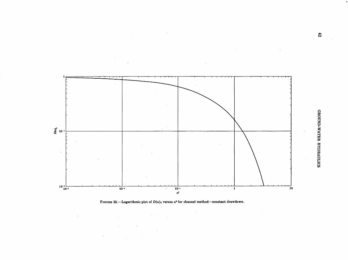
42G
RO
UN
D-W
AT
ER
HY
DR
AU
LIC
S
Io1 §1Is
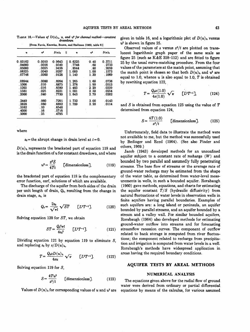
AQUIFER TESTS BY AREAL METHODS 43
TABLE 16. Values of D(u) h, u, and u1 for channel method constantdrawdown
[From Ferris, Knowles, Brown, and Stallman (1962, table 6)]
w« />(«)* II
0.03162.04000.05000.06325.07746
.08944
.1000
.1265
.1581
.2000
.2449
.2828
.3162
.4000
.5000
0.0010.0016.0025.0040.0060
.0080
.010
.016
.025
.040
.060
.080
.10
.16
.25
0.9643.9549.9436.9287.9128
.8994
.8875
.8580
.8231
.7730
.7291
.6892
.6548
.5716
.4795
0.6325.7746.8944
1.0001.140
1.2651.3781.4831.5811.643
1.7321.789
0.40.60.80
1.001.30
1.601.902.202.502.70
3.003.20
0.3711.2733.2059.1573.1069
.0736
.0513
.0359
.0254
.0202
.0143
.0114
where
So=the abrupt change in drain level at < = 0.
D(u)h represents the bracketed part of equation 118 and is the drain function of u for constant drawdown, and where
w2 = [dimensionless], (119)Tt-£ v
the bracketed part of equation 118 is the complementary error function, cerf, solutions of which are available.
The discharge of the aquifer from both sides of the drain per unit length of drain, Qb , resulting from the change in drain stage, so, is
Solving equation 120 for ST, we obtain
3T ^ Qflrf4s02
(120)
(121)
Dividing equation 121 by equation 119 to eliminate S, and replacing s0 by s/D(u)h,
T-
Solving equation 119 for S,
47V S= [dimensionless].
X j L
(122)
(123)
given in table 16, and a logarithmic plot of D(u)h versus w2 is shown in figure 25.
Observed values of s versus x*/t are plotted on trans lucent logarithmic graph paper of the same scale as figure 25 (such as K&E 358-112) and are fitted to figure 25 by the usual curve-matching procedure. From the four values of the parameters at the match point, assuming that the match point is chosen so that both D(u)h and w2 are equal to 1.0, whence u is also equal to 1.0, T is obtained by rewriting equation 122,
.0)(124)
and S is obtained from equation 123 using the value of T determined from equation 124,
47X1.0)[dimensionless]. (125)
Values of D(u}h for corresponding values of u and it2 are
Unfortunately, field data to illustrate the method were not available to me, but the method was successfully used by Bedinger and Reed (1964). (See also Finder and others, 1969.)
Jacob (1943) developed methods for an unconfined aquifer subject to a constant rate of recharge (W) and bounded by two parallel and assumedly fully penetratingstreams. The base flow of streams or the average rate of ground-water recharge may be estimated from the shape of the water table, as determined from water-level meas urements in wells, in such a bounded aquifer. Rorabaugh (1960) gave methods, equations, and charts for estimating the aquifer constant T/S (hydraulic diffusivity) from natural fluctuations of water levels in observation wells in finite aquifers having parallel boundaries. Examples of such aquifers are: a long island or peninsula, an aquifer bounded by parallel streams, and an aquifer bounded by a stream and a valley wall. For similar bounded aquifers, Rorabaugh (1964) also developed methods for estimating ground-water outflow into streams and for forecasting streamflow recession curves. The component of outflow related to bank storage is computed from river fluctua tions; the component related to recharge from precipita tion and irrigation is computed from water levels in a well. Rorabaugh's methods have widespread application in areas having the required boundary conditions.
AQUIFER TESTS BY AREAL METHODS
NUMERICAL ANALYSIS
The equations given above for the radial flow of ground water were derived from ordinary or partial differential equations by means of the calculus, for various assumed
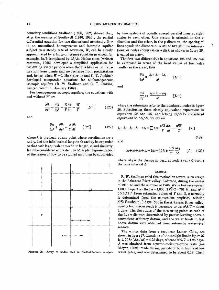
44 GROUND-WATER HYDRAULICS
boundary conditions. Stallman (1956, 1962) showed that, after the manner of Southwell (1940, 1946), the partial differential equation for two-dimensional nonsteady flow in. an unconfined homogeneous and isotropic aquifer subject to a steady rate of accretion, W, can be closely approximated by a finite-difference equation in which, for example, dh/dt is replaced by hh/ht. He has since (written commun., 1965) developed a simplified application for use during winter periods when there is little or no trans piration from plants and no recharge from precipitation and, hence, when W = Q. He (later he and C. T. Jenkins) developed comparable equations for nonhomogeneous isotropic aquifers (R. W. Stallman and C. T. Jenkins, written commun., January 1969).
For homogeneous isotropic aquifers, the equations with and without W are
(126)
and
, = _ dx2 dy*~ Tdt T L
= dx2 dy2 ~ Tdt L
where h is the head at any point whose coordinates are x and y. Let the infinitesimal lengths dx and dy be expanded so that each is equivalent to a finite length, a, and similarly, let dt be considered equivalent to M. A plan representation of the region of flow to be studied may then be subdivided
by two systems of equally spaced parallel lines at right angles to each other. One system is oriented in the x direction and the other, in the y direction; the spacing of lines equals the distance a. A set of five gridline intersec tions, or nodes (observation wells), as shown in figure 26, is called an array.
The first two differentials in equations 126 and 127 can be expressed in terms of the head values at the nodes (wells) in the array, thus
[IT']
and
o ri ti% ~T~ h/4 ^h/Q dy2 a2
where the subscripts refer to the numbered nodes in figure 26. Substituting these closely equivalent expressions in equations 126 and 127, and letting dh/dt be considered equivalent to A/i0/A<, we obtain
a?W
and(128)
(129)
FIGURE 26. Array of nodes used in finite-difference analysis.
where AA0 is the change in head at node (well) 0 during the time interval At.
EXAMPLE
R. W. Stallman tried this method on several such arrays in the Arkansas River valley, Colorado, during the winter of 1965-66 and the summer of 1966. Wells 1-4 were spaced 1,000ft apart so that a = 1,000 ftV§/2 = 707 ft, and a2 = 5X105 ft2 . From estimated values of T and S, a normally is determined from the convenient empirical relation a?S/T= about 10 days, but in the Arkansas River valley, nearby boundaries made it necessary to use a?S/ T = about4 days. The elevations of the measuring points at each of the five wells were determined by precise leveling above a convenient arbitrary datum, and the water levels in feet above datum were obtained from automatic water-level sensors.
The winter data from a test near Lamar, Colo., are shown in figure 27. The slope of the straight line in figure 27 is A £ h/(Ah0/M) =4.25 days, whence a2£/77 = 4.25 days.5 was obtained from neutron-moisture-probe tests (see Meyer, 1962), made during periods of both high and low water table, and was determined to be about 0.18. Then,
45
using equation 129,
a?S (5X105 ft2)(0.18) 4.25 days
«2 X104 ft2 day-1 (rounded).
The straight line in figure 27 has been transferred to the plot of spring and summer data shown in figure 28. In figure 28, points to the right of the straight line indicating W = 0 show recharge to the water table; those to the left show discharge from the water table by evapotranspiration. The average value of £} h above the line is about 0.1 ft. Using 7T«2X104 ft2 day-1 and a2 = 5X105 ft2 , from equa tion 128,
O.lft«-(5X105 ft2 )(KQ 2X104 ft2 day~1
and
( _ (2X104 ft2 day-1 )(0.1ft) 5X10^ ft2
: - 4 X 10~3 ft day-1 (rounded).
FLOW-NET ANALYSIS
The following discussion of flow-net analysis has been adapted in part from Bennett (1962) and from Bennett and Meyer (1952, p. 54-58), to whose reports you are referred for further details.
In analyzing problems of steady ground-water flow, a graphical representation of the flow pattern may be of considerable assistance and may provide solutions to problems not readily amenable to mathematical solution. The first significant development in graphical analysis of flow patterns was made by Forchheimer (1930), but additional information was given by Casagrande (1937, p. 136, 137) and Taylor (1948).
A flow net, which is a graphical illustration of a flow pattern, is composed of two families of lines or curves. (See fig. 30.) One family of curves, called equipotential lines (solid lines on map), represents contours of equal head in the aquifer on the potentiometric surface or on the water table. Intersecting the equipotential lines at right angles (in isotropic aquifers) is another family of curves (dashed lines on map) representing the streamlines, or flow lines, where each curve indicates the path followed by a particle (molecule) of water as it moves through the aquifer in the direction of decreasing head.
Although the real flow pattern contains an infinity of possible flow and equipotential lines, it may be represented conveniently by constructing a net that uses only a few such lines, the spacing being conveniently determined by
the contour interval of the equipotential lines. The con tour interval indicates that the total drop in head in the system is evenly divided between adjacent pairs of equipotential lines; similarly the flow lines are selected so that the total flow is equally divided between adjacent pairs of flow lines. The movement of each particle of water between adjacent equipotential lines will be along flow paths involving the least work, hence it follows that, in isotropic aquifers, such flow paths will be normal to the equipotential lines, and the paths are drawn orthogonal to the latter.
The net is constructed so that the two sets of lines form a system of "squares." Note on the map that some of the lines are curvilinear, but that the "squares" are constructed so that the sum of the lengths of each line in one system is closely equal to the sum of the lengths in the other system. Figure 29 represents one idealized "square" of figure 30, whose dimensions are Aw and AZ. By rewriting Darcy's law (eq. 26) as a finite-difference equation for the flow, AQ, through this elemental "square" of thickness 6, we obtain
A/i AAAQ = -Kb&w =- TAw A/ At
But Aw = AZ, by construction, so
-1]. (130)
[L*T~l ~\. (131)
If nf = number of flow channels, nd = number of potential drops, and Q = total flow, then
and
, or A<?= -nf
or AA= [L~\. nd
(132)
(133)
Substituting equations 132 and 133 in equation 131, we obtain
(134)
or
Q(nf/nd}h
(135)
EXAMPLE
According to Bennett and Meyer (1952, p. 55), the average discharge from the Patuxent Formation in the Sparrows Point district in 1945 was 1 million ft8 day"1 . The map (fig. 30) shows 15 flow channels surrounding the
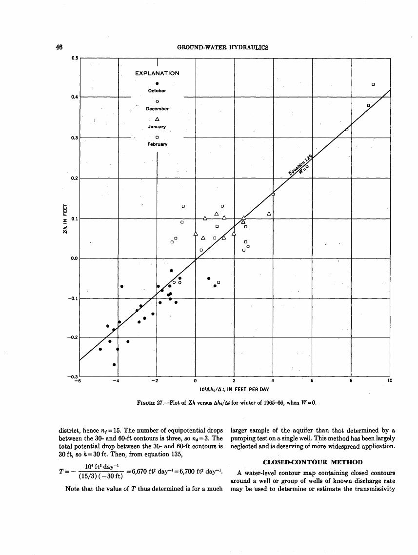
46 GROUND-WATER HYDRAULICS
0.5
0.4
0.3
0.2
EXPLANATION
October
o
December
A
January
o
February
0.1
0.0
-0.1
-0.2
-0.3-6 -2 024
102Afc0 /A t, IN FEET PER DAY
FIGURE 27. Plot of Sfc versus AA0/AJ for winter of 1965-66, when W=0.
10
district, hence n/= 15. The number of equipotential drops between the 30- and 60-ft contours is three, so n<j = 3. The total potential drop between the 30- and 60-ft contours is 30 ft, so h = 30 ft. Then, from equation 135,
IO6 ft 3 dav"1T= - =6'670 ft° d<*-'= 6'700 ft°(is/3) (-
Note that the value of T thus determined is for a much
larger sample of the aquifer than that determined by a pumping test on a single well. This method has been largely neglected and is deserving of more widespread application.
CLOSED-CONTOUR METHOD
A water-level contour map containing closed contours around a well or group of wells of known discharge rate may be used to determine or estimate the transmissivity
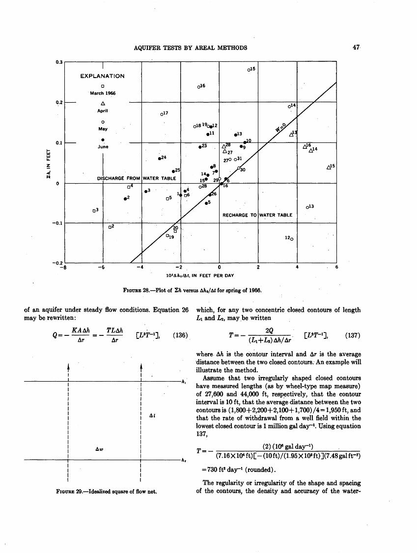
AQUIFER TESTS BY AREAL METHODS 47
U.d
0.2
0.1
0
-0.1
EXPLArNATION
aMarch 1966
A April
0May
June
Dl
03
CHARGE FROM
D4
2
02
017
.24
25
WATER TABLE
^* 1,
05
,
/?&s D
016
19° O*12
11
23
«
14. 7*
15* 29<
4 °28 /*6 w^6
/ s/
/
0«
13
.. ,10A28 "^27 >
?7O o31 >r
oXv^0L«
16
RECHARGE TO
°14
/
$s/ d3/s'
WATER TABLE
120
s
//
^16A14
^15
013
-0.2 -8 -6 -4-2 0 2 4
10 2 Afc0 /A«. IN FEET PER DAY
FIGURE 28. Plot of Sfc versus Afc 0/A« for spring of 1966.
of an aquifer under steady flow conditions. Equation 26 which, for any two concentric closed contours of length may be rewritten: LI and Lv, may be written
KAtfi
ArTLAfe
Ar
Aw
FIGURE 29. Idealized square of flow net.
-A.
T=- (137)
where AJi is the contour interval and Ar is the average distance between the two closed contours. An example will illustrate the method.
Assume that two irregularly shaped closed contours have measured lengths (as by wheel-type map measure) of 27,600 and 44,000 ft, respectively, that the contour interval is 10 ft, that the average distance between the two contours is (1,800+2,200+2,100+1,700) /4 = 1,950 ft, and that the rate of withdrawal from a well field within the lowest closed contour is 1 million gal day"1 . Using equation 137,
T=- (2) (106 gal day1 )(7.16X104 ft)[-(10ft)/(1.95X108 ft)](7.48galft-»)
= 730 ft2 day-1 (rounded).
The regularity or irregularity of the shape and spacing of the contours, the density and accuracy of the water-
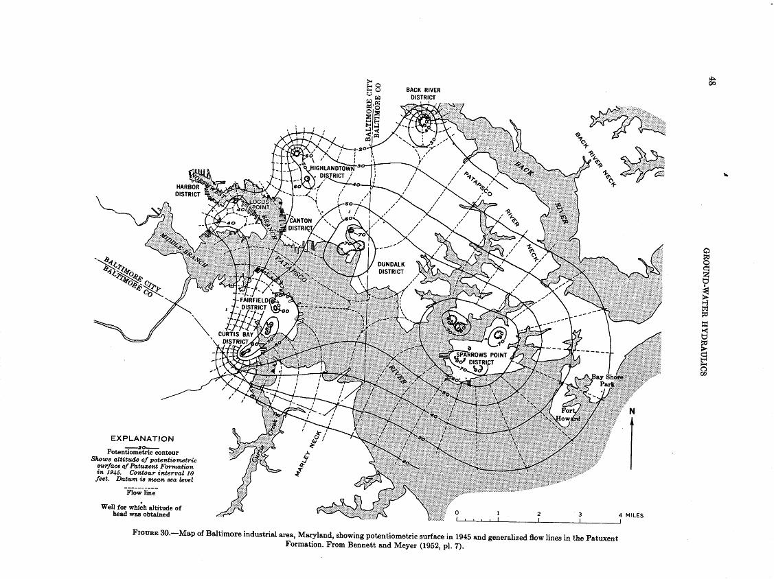
EXPLANATION
Potentiometric contourShows altitude of potentiometric
surface of Patuxent Formationin 1945. Contour interval 10feet. Datum is mean sea level
Flow line
Well for which altitude of head was obtained 4 MILES
O
1 I&
a
FIGURE 30. Map of Baltimore industrial area, Maryland, showing potentiometric surface in 1945 and generalized flow lines in the PatuxentFormation. From Bennett and Meyer (1952, pi. 7),
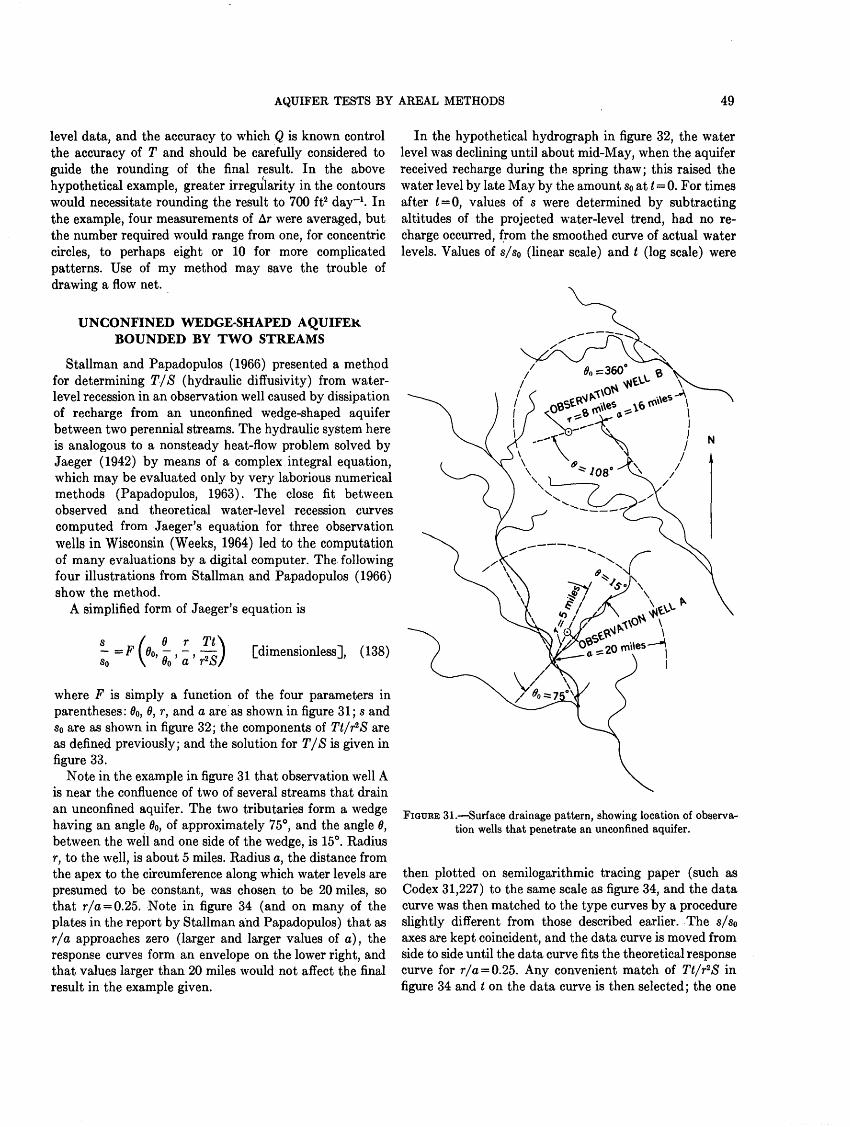
AQUIFER TESTS BY AREAL METHODS 49
level data, and the accuracy to which Q is known control the accuracy of T and should be carefully considered to guide the rounding of the final result. In the above hypothetical example, greater irregularity in the contours would necessitate rounding the result to 700 ft2 day1 . In the example, four measurements of Ar were averaged, but the number required would range from one, for concentric circles, to perhaps eight or 10 for more complicated patterns. Use of my method may save the trouble of drawing a flow net.
UNCONFINED WEDGE-SHAPED AQUIFER BOUNDED BY TWO STREAMS
Stallman and Papadopulos (1966) presented a method for determining T-/S (hydraulic diffusivity) from water- level recession in an observation well caused by dissipation of recharge from an unconfined wedge-shaped aquifer between two perennial streams. The hydraulic system here is analogous to a nonsteady heat-flow problem solved by Jaeger (1942) by means of a complex integral equation, which may be evaluated only by very laborious numerical methods (Papadopulos, 1963). The close fit between observed and theoretical water-level recession curves computed from Jaeger's equation for three observation wells in Wisconsin (Weeks, 1964) led to the computation of many evaluations by a digital computer. The following four illustrations from Stallman and Papadopulos (1966) show the method.
A simplified form of Jaeger's equation is
[dimensionless], (138)
where F is simply a function of the four parameters in parentheses: 0o, 0, r, and a are as shown in figure 31; s and «o are as shown in figure 32; the components of Tt/r2S are as defined previously; and the solution for T/S is given in figure 33.
Note in the example in figure 31 that observation well A is near the confluence of two of several streams that drain an unconfined aquifer. The two tributaries form a wedge having an angle do, of approximately 75°, and the angle 6, between the well and one side of the wedge, is 15°. Radius r, to the well, is about 5 miles. Radius a, the distance from the apex to the circumference along which water levels are presumed to be constant, was chosen to be 20 miles, so that r/a = 0.25. Note in figure 34 (and on many of the plates in the report by Stallman and Papadopulos) that as r/a approaches zero (larger and larger values of a), the response curves form an envelope on the lower right, and that values larger than 20 miles would not affect the final result in the example given.
In the hypothetical hydrograph in figure 32, the water level was declining until about mid-May, when the aquifer received recharge during the spring thaw; this raised the water level by late May by the amount So at i = 0. For times after £ = 0, values of s were determined by subtracting altitudes of the projected water-level trend, had no re charge occurred, from the smoothed curve of actual water levels. Values of S/SQ (linear scale) and t (log scale) were
FIGURE 31. Surface drainage pattern, showing location of observa tion wells that penetrate an unconfined aquifer.
then plotted on semilogarithmic tracing paper (such as Codex 31,227) to the same scale as figure 34, and the data curve was then matched to the type curves by a procedure slightly different from those described earlier. The s/s0 axes are kept coincident, and the data curve is moved from side to side until the data curve fits the theoretical response curve for r/a = 0.25. Any convenient match of Tt/r*S in figure 34 and t on the data curve is then selected; the one

50 GROUND-WATER HYDRAULICS
30
25
UJQ
20
15
10
t=0e =15r = 5 miles a = 20 miles
Observed water-level altitudes (smoothed)
Projected water-level trend
Jan Feb Mar Apr May June July Aug Sept Oct Nov Dec
FIOUBB 32. Example hydrograph from well A of figure 31, showing observed and projected water-level altitudes.
chosen in the example in figure 33 was for Tt/r*S=l.Q and < = 360days. From the value Tt/i*S=*l.O, T/S = l.QXr*/t= 1.0X6.98X108 ft2/360 days = 1.94X106 ft2 day-1 . If S is known or estimated to be, say 0.2, then 7T =0.2X1.94X106 ft2 day1 = about 4X105 ft2 day-1 . Note that in figure 34,
0.2
0.4
0.6
0.8
i.o
i 1111 i i r *>"''
/ Observed /theoretical response
Match line atJtt-u»
t= 360 days Computation:
T 1.00x6.98xl0 8n
10 100
t. IN DAYS
1000
FIGURE 33. «/«», versus t taken from hydrograph of well A (see fig. 32), showing computation of T/S.
which is a nondimensional plot, Stallman and Papadopulos omitted the pure number 4 from the numerator of Tt/r^S, thus eliminating the necessity of using it in computations.
In the hypothetical data plotted in figures 32 and 33, values of s/s0 were plotted for t from 5 to 200 days, but the authors warn that in actual practice it would be difficult to reliably project the water-level trend much beyond July and that, in general, values of s/*o for only about 50 days after cessation of recharge should be considered useful.
Note in figure 31 that observation well B is considered to be within a circular area of 0o = 360° and a radius of 16 miles surrounded by streams but that only the stream at 0=108° was considered. R. W. Stallman (U.S. Geological Survey, oral commun., 1968) indicated that this rather extreme example might be improved by reducing radius a to about 12 miles, so that it just intersects the streams to the northwest, west, and south.
Figure 34 is but one of 120 sheets containing in all some 1,500 response curves for various values of 00,0/0o, and r/a. This method should have widespread application in many places where unconfined aquifers are traversed by perennial streams, and where at least a few wells are available for observation of water levels preceding and following periods of recharge. In some studies this method might provide the only values of T/S and estimates of T; in others, it could conveniently supplement values obtained by other

AQ
UIFE
R T
EST
S BY
AR
EAL M
ET
HO
DS
51
^ «2
"! "*
CO«
v.
:?<
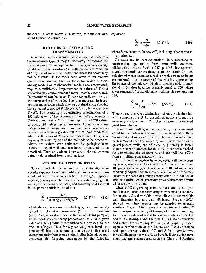
52 GROUND-WATER HYDRAULICS
methods. In areas where T is known, this method also could be used to estimate S.
METHODS OF ESTIMATING TRANSMISSIVITY
In some ground-water investigations, such as those of a reconnaissance type, it may be necessary to estimate the transmissivity of an aquifer from the specific capacity (yield per unit of drawdown) of wells, as the determination of T by use of some of the equations discussed above may not be feasible. On the other hand, some of our modern quantitative studies, such as those for which electric- analog models or mathematical models are constructed, require a sufficiently large number of values of T that transniissivity-contour maps (T maps) may be constructed. In unconfined aquifers, such T maps generally require also the construction of water-level contour maps and bedrock- contour maps, from which may be obtained maps showing lines of equal saturated thickness, b, for we have seen that T = Kb. For example, a quantitative investigation of a 150-mile reach of the Arkansas River valley, in eastern Colorado, required a T map based upon about 750 values, or about 1% values per square mile. About 25 of these values were obtained from pumping tests, selected as reliable tests from a greater number of tests conducted. About 200 values of T were estimated from the specific capacity of wells, by one of the methods to be described. About 525 values were estimated by geologists from studies of logs of wells and test holes, by methods to be described. Thus, only about 3 percent of the values were actually determined from pumping tests.
SPECIFIC CAPACITY OF WELLS
Several methods for estimating transmissivity from specific capacity have been published, some of which are cited below. If we solve equation 51 for Q/sw (specific capacity), using sw as the drawdown in the discharging well, and rw as the radius of the well, and assuming that the well is 100 percent efficient, we obtain
equation:
3.Sin 2.301ogio 2.25Tt/rw*S
(139)
which shows the manner in which Q/sw is approximately related to the other constants (T, S) and variables (rw , t). As rw is constant for a particular well being pumped, we see that Q/sw is nearly proportional to T7 at a given value of t, but gradually diminishes as t increases, by the amount 1/logio t. Thus, for a given well, considered 100- percent efficient, and assuming that water is discharged instantaneously from storage with decline in head, we may symbolize the foregoing statements by the following
Q Blogic t
(140)
where B = a constant for the well, including other terms as in equation 139.
No wells are 100-percent efficient, but, according to construction, age, and so forth, some wells are more efficient than others. Jacob (1947, p. 1048) has approxi mated the head loss resulting from the relatively high velocity of water entering a well or well screen as being proportional to some power of the velocity approaching the square of the velocity, which in turn is nearly propor tional to Q2 ; thus head loss is nearly equal to CQ2, where C = a constant of proportionality. Adding this to equation 140,
Q Blogic t
+CQ2 (141)
Thus we see that Q/sw diminishes not only with time but with pumping rate Q. In unconfined aquifers it may be necessary to adjust factor B further to account for delayed yield from storage.
In an uncased well in, say, sandstone, rw may be assumed equal to the radius of the well, but in screened wells in unconsolidated material, in which the finer particles have been removed near the screen by well development, or in gravel-packed wells, the effective rw generally is larger than the screen diameter. Jacob (1947) described a method for determining the effective rw and the well loss (CQ2 ) from a multiple-step drawdown test.
Most other investigators have neglected well loss in their equations, which are then equations for wells of assumed 100 percent efficiency, such as equation 140, but some have arbitrarily adjusted for this loss by selection of an arbitrary constant for wells of similar construction in a particular area or aquifer, which generally gives satisfactory results when used with caution.
Theis (1963a) gave equations and a chart, based upon the Theis equation, for estimating T from specific capacity for constant S and variable t, with allowance for variable well diameter but not well efficiency. Brown (1963) showed how Theis' results may be adapted to artesian aquifers. Meyer (1963) gave a chart for estimating T from the specific capacity at the end of 1 day of pumping, for different values of S and for well diameters of 0.5, 1.0, and 2.0ft. Bedinger and Emmett (1963) gave equations and a chart for estimating T from specific capacity, based upon a combination of the Thiem and Theis equations and upon average values of T and S for a specific area, for well diameters of 0.5, 1.0, and 2.0 ft. Hurr (1966) gave equations and charts based upon the Theis and Boulton
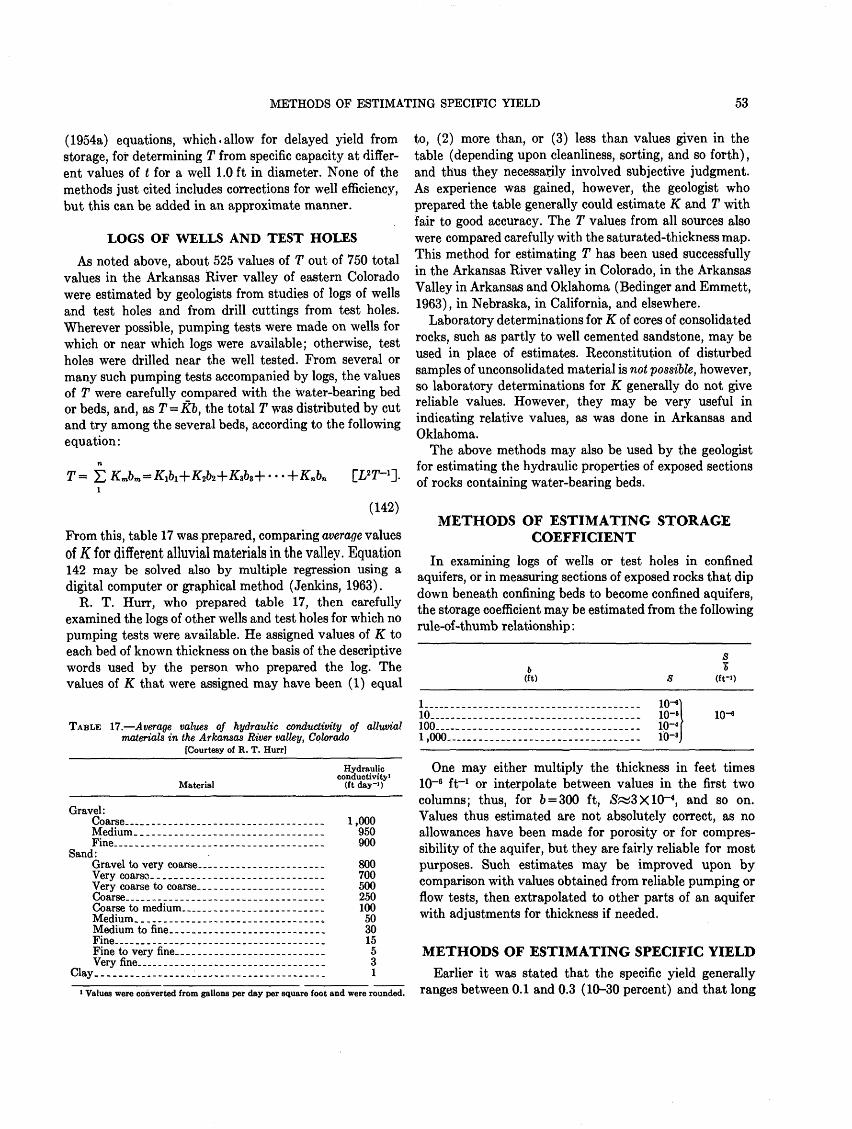
METHODS OF ESTIMATING SPECIFIC YIELD 53
(1954a) equations, which. allow for delayed yield from storage, for determining T from specific capacity at differ ent values of t for a well 1.0 ft in diameter. None of the methods just cited includes corrections for well efficiency, but this can be added in an approximate manner.
LOGS OF WELLS AND TEST HOLES
As noted above, about 525 values of T out of 750 total values in the Arkansas River valley of eastern Colorado were estimated by geologists from studies of logs of wells and test holes and from drill cuttings from test holes. Wherever possible, pumping tests were made on wells for which or near which logs were available; otherwise, test holes were drilled near the well tested. From several or many such pumping tests accompanied by logs, the values of T were carefully compared with the water-bearing bed or beds, and, as T=Kb, the total T was distributed by cut and try among the several beds, according to the following equation:
T = Kmbm = Kj>l +Kjb»+KjH+ +Knbn
(142)
From this, table 17 was prepared, comparing average values of K for different alluvial materials in the valley. Equation142 may be solved also by multiple regression using a digital computer or graphical method ( Jenkins, 1963) .
R. T. Hurr, who prepared table 17, then carefully examined the logs of other wells and test holes for which no pumping tests were available. He assigned values of K to each bed of known thickness on the basis of the descriptive words used by the person who prepared the log. The values of K that were assigned may have been (1) equal
TABLE 17. Average values of hydraulic conductivity of alluvialmaterials in the Arkansas River valley, Colorado
[Courtesy of R. T. Hurr]
Material
Gravel:
Medium. __.__.._____.._____..___Fine.. ........_..........._......
Sand: Gravel to very coarse _ . .-------..
Very coarse to coarse. ..---------.-Coarse __ ._-__-_-..__-._-..__.--Coarse to medium __ _....._......Medium, ........................Medium to fine. ---.__---.--_--_..Fine... ........._................Fine to very fine.---.--------.----Very fine __ --------------_-_._-_
Clay................................
Hydraulic conductivity'
(ft day-")
......... 1,000
......... 950
......... 900
......... 800
......... 700- _-.__ 500......... 250......... 100......... 50......... 30......... 15......... 5......... 3 .. . 1
to, (2) more than, or (3) less than values given in the table (depending upon cleanliness, sorting, and so forth), and thus they necessarily involved subjective judgment. As experience was gained, however, the geologist who prepared the table generally could estimate K and T with fair to good accuracy. The T values from all sources also were compared carefully with the saturated-thickness map. This method for estimating T has been used successfully in the Arkansas River valley in Colorado, in the Arkansas Valley in Arkansas and Oklahoma (Bedinger and Emmett, 1963), in Nebraska, in California, and elsewhere.
Laboratory determinations for K of cores of consolidated rocks, such as partly to well cemented sandstone, may be used in place of estimates. Reconstitution of disturbed samples of unconsolidated material is not possible, however, so laboratory determinations for K generally do not give reliable values. However, they may be very useful in indicating relative values, as was done in Arkansas and Oklahoma.
The above methods may also be used by the geologist for estimating the hydraulic properties of exposed sections of rocks containing water-bearing beds.
METHODS OF ESTIMATING STORAGE COEFFICIENT
In examining logs of wells or test holes in confined aquifers, or in measuring sections of exposed rocks that dip down beneath confining beds to become confined aquifers, the storage coefficient may be estimated from the following rule-of-thumb relationship:
b(ft)
1...... ......._........ ..........10...............................100. ..........................1,000 . ........................
s
........ 10r*\
........ 10-M
........ 10-* f
........ io-8j
S b
(ft'')
io-«
> Values were converted from gallons per day per square foot and were rounded.
One may either multiply the thickness in feet times 10~6 ft"1 or interpolate between values in the first two columns; thus, for 6 = 300 ft, £«3X10~4 , and so on. Values thus estimated are not absolutely correct, as no allowances have been made for porosity or for compres sibility of the aquifer, but they are fairly reliable for most purposes. Such estimates may be improved upon by comparison with values obtained from reliable pumping or flow tests, then extrapolated to other parts of an aquifer with adjustments for thickness if needed.
METHODS OF ESTIMATING SPECIFIC YIELDEarlier it was stated that the specific yield generally
ranges between 0.1 and 0.3 (10-30 percent) and that long
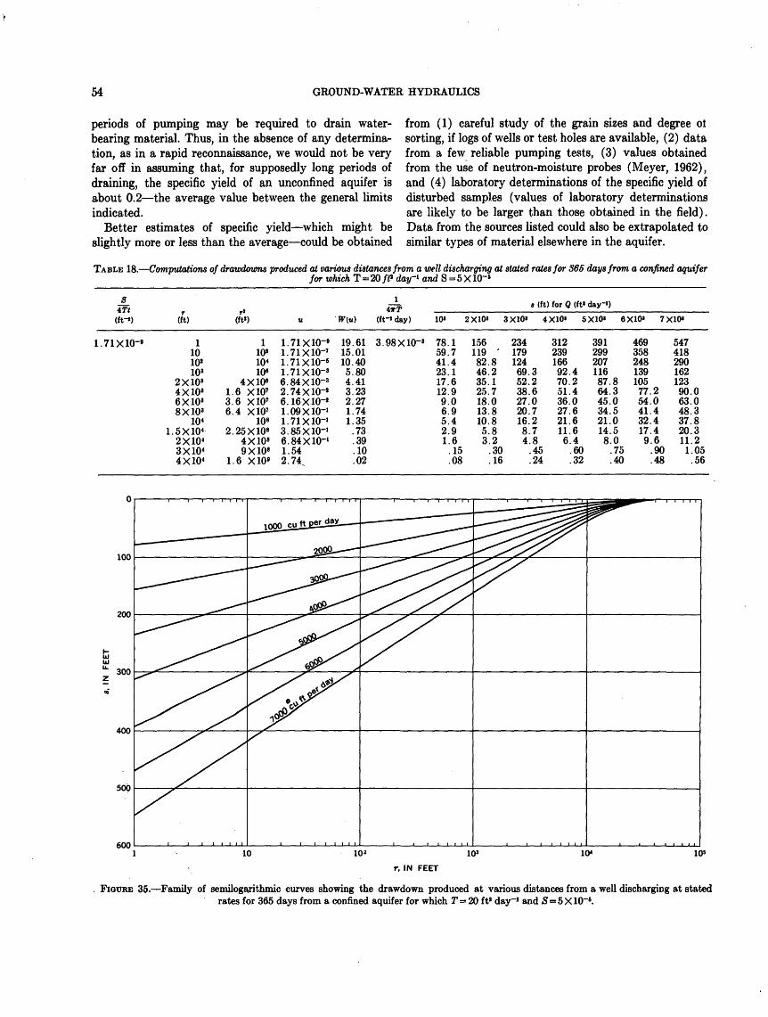
54 GROUND-WATER HYDRAULICS
periods of pumping may be required to drain water bearing material. Thus, in the absence of any determina tion, as in a rapid reconnaissance, we would not be very far off in assuming that, for supposedly long periods of draining, the specific yield of an unconfined aquifer is about 0.2 the average value between the general limits indicated.
Better estimates of specific yield which might be slightly more or less than the average could be obtained
from (1) careful study of the grain sizes and degree ot sorting, if logs of wells or test holes are available, (2) data from a few reliable pumping tests, (3) values obtained from the use of neutron-moisture probes (Meyer, 1962), and (4) laboratory determinations of the specific yield of disturbed samples (values of laboratory determinations are likely to be larger than those obtained in the field). Data from the sources listed could also be extrapolated to similar types of material elsewhere in the aquifer.
TABLE 18. Computations of drawdowns produced at various distances from a well discharging at stated rates for 865 days from a confined aquiferfor which T=20 ft8 day'1 and S=5 X 10~5
S 4Tt r (ft-*) (ft)
1.71X10-* 11010*103
2X10"4X10'6X10"8X10³
10«1.5X10⁴
2X1043X10<4X10<
T*
(ft»)
110s10<10"
4X1081.6 X1073.6 X1076.4 X107
10"2.25X10⁸
4X1089X10"
1.6 X10»
V
1.71X10-*1.71X10-71.71X10-61.71X10-'6.84X10⁻³². 74X10-*6. 16X10-*1.09X10-'1.71X10"13.85X10-16.84X10-11.542.74
1 4nrT
W(u) (ff« day)
1915.10.5.4.3211
.61 3. 98X10-'
.01408041
.23
.27
.74
.35
.73
.39
.10
.02
« (ft) for Q (ft* day-«)
10» 2X10» 3X10» 4X10» 5X10« 8X10» 7X10»
78.159.741.423.117.612.99.06.95.42.91.6
.15
.08
156119 '82.846.235.125.718.013.810.85.83.2
.30
.16
23417912469.352.238.627.020.716.28.74.8
.45
.24
31223916692.470.251.436.027.621.611.66.4
.60
.32
39129920711687.864.345.034.521.014.58.0
.75
.40
46935824813910577.254.041.432.417.49.6
.90
.48
54741829016212390.063.048.337.820.311.21.05
.56
100
200
300
400
500
600103 10*
r. IN FEET
105
FIGURE 35. Family of semilogarithmic curves showing the drawdown produced at various distances from a well discharging at stated rates for 365 days from a confined aquifer for which T = 20 ft* day"1 and S=5X 10"B.
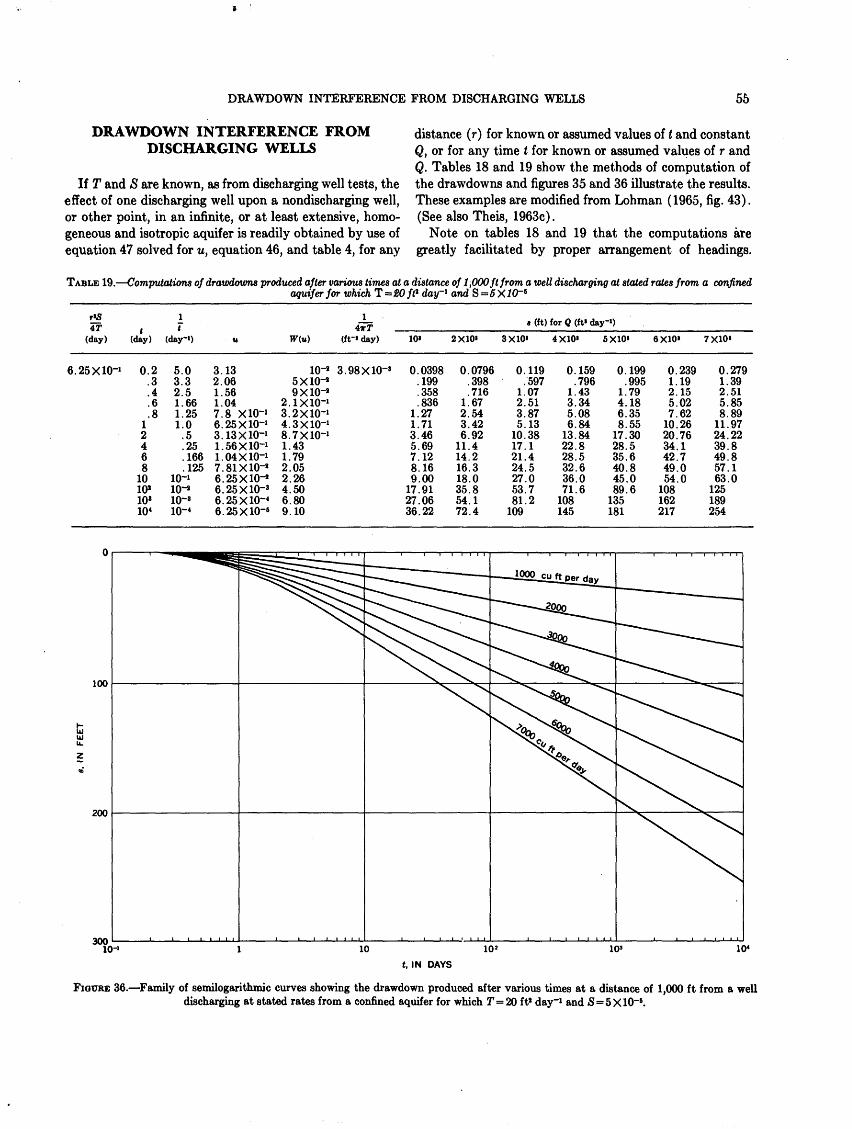
DRAWDOWN INTERFERENCE FROM DISCHARGING WELLS 56
DRAWDOWN INTERFERENCE FROM DISCHARGING WELLS
If T and S are known, as from discharging well tests, the effect of one discharging well upon a nondischarging well, or other point, in an infinite, or at least extensive, homo geneous and isotropic aquifer is readily obtained by use of equation 47 solved for u, equation 46, and table 4, for any
distance (r) for known or assumed values of t and constant Q, or for any time t for known or assumed values of r and Q. Tables 18 and 19 show the methods of computation of the drawdowns and figures 35 and 36 illustrate the results. These examples are modified from Lohman (1965, fig. 43). (See also Theis, 1963c).
Note on tables 18 and 19 that the computations are greatly facilitated by proper arrangement of headings.
TABLE 19. Computations of drawdowns produced after various times at a distance of 1,000 ft from a well discharging at stated rates from a confinedaquifer for which T=20ft* day-1 and S=6X10~S
r«S 1 4r i <
(day) (day) (day"1) u
j?p « (ft) for Q (ft» day'1)
W(u) (ff«day) 10» 2X10» 3X10» 4X10« 5X10» 6X10» 7X10»
6.25X10-' 0.2 5.0 3.13 3.98X10-' 0.0398 0.0796 0.119 0.159 0.199 0.239 0.279.3.4.6.8
12468
1010110*10<
3.32.51.661.251.0
.5
.25
.166
.12510-'10"810~'io-<
2.061.561.047.8 X10-'6.25X10-'3.13X10-'1.56X10-'1.04X10-'7.81X10-'6. 25X10-*6.25X10-'6.25X10-46.25X10-8
5X10-29X10-1
2.1X10-'3.2X10-'4.3X10-'8.7X10-'1.431.792.052.264.506.809.10
1.1.3.5.7.89
172736
199358836277146.6912
.16
.00
.91
.06
.22
.398
.7161.672.543.426.92
11.414.216.318.035.854.172.4
.5971.072.513.875.13
10.3817.121.424.527.053.781.2
109
.7961.433.345.086.84
13.8422.828.532.636.071.6
108145
.9951.794.186.358.55
17.3028.535.640.845.089.6
135181
1.192.155.027.62
10.2620.7634.142.749.054.0
108162217
1.392.515.858.89
11.9724.2239.849.857.163.0
125189254
300
t, IN DAYS
FIGURE 36. Family of semilogarithmic curves showing the drawdown produced after various times at a distance of 1,000 ft from a well discharging at stated rates from a confined aquifer for which T= 20 ft* day"1 and 5=5 X10"8.

56 GROUND-WATER HYDRAULICS
Thus, single values of S/±Tt or r*S/4T multiplied by various values of r2 or l/t, respectively, give values of u from which values of W(u) are obtained from table 5. Then, a single value of l/4irT multiplied by various values of W(u] and by Q = 103 ft3 day"1 gives the drawdowns for this discharge rate. Then the drawdowns for other values of Q are obtained by simple multiplication by 2 through 7. Note that only a few values establish the straight-line parts of the curves but that more are required for the curvilinear parts.
The examples just given are for constant discharge and variable drawdown, but other equations for different boundary conditions could be similarly used to determine drawdown interference. Thus, for example, equations 66 and 67 and table 7 could be used for discharging wells of constant drawdown and variable discharge. In these examples, discharging wells constitute hydraulic bound aries of the point-sink type; recharging wells constitute boundaries of the point-source type. Other types of boundaries are discussed in later sections.
Figures 35 and 36 show only the drawdown caused by one discharging well at a nondischarging well or point within the cone of depression. Where many discharging wells are mutually interfering with each other and with other points, such as nondischarging wells, the problem becomes much more complex and is best handled by an electric analog-model computer or by a digital computer. The drawdown interference from certain groupings of discharging wells is treated by Hantush (1964, p. 374-382).
RELATION OF STORAGE COEFFICIENT TO SPREAD OF CONE OF DEPRESSION
It has been shown (Lohman, 1965, p. 109, 110) that if equation 51 is solved for r2, there results
2.25T*(143)
For a given set of conditions, all terms except r2 and S may be considered constant; then, using C as a constant of proportionality,
(144)
For convenience, multiply both sides of equation 144 by TT, then
(145)
As an example, equation 145 may be used to compare the area of influence, AI, in a confined aquifer having a storage coefficient of, say 5X10~5, with the area of influence, A 2 , in an uriconfined aquifer having a specific yield of, say 0.20. Assuming that T, Q, and s are the same for both aquifers, and that t also is the same and is long enough so that w<0.01 and that the material in the cone of depression in the unconfined aquifer has had time to be drained, then
C75X1Q-5
C70.20= 4X10³ .
Thus, under the assumed conditions, the area of in fluence in the confined aquifer is 4,000 times larger than that in the unconfined aquifer, or the ratio of the radius extending to the circumference of negligible drawdown in the confined aquifer to that in the unconfined aquifer, ri/r2 , is \/4X103 = 63.2. Thus, changes in water level in a confined aquifer spread outward very rapidly from a dis charging well, whereas in an unconfined aquifer changes in water level spread very slowly as gravity drainage takes place.
Dischai \ rgmg welkj\ [uandsurfai
> Impermeable or ' > 4 confining mat rial r * v
or effective position of line of zero flow
A. REAL SYSTEM
Drawdown componentof image well
Discharging Q real wel **
Drawdown component of real well
Q Discharging
' ' ' : ' ' '. '. ' ' :' ' ] \: .'Aquifer'.'. . :' '.;:-/..: .:":':'.' ; : .' i'.'l V:". :l::::':':::'.: ' ': : ' ' '. - ; - '
where A = area of influence.
NOTE: Aquifer thickness b should be very large compared to resultant drawdown near real well
B. HYDRAULIC COUNTERPART OF REAL SYSTEM
FIGURE 37. Idealized section views of a discharging well in an aquifer bounded by an "impermeable" barrier and of the equiva lent hydraulic system in an infinite aquifer. From Ferris, Knowles, Brown, and Stallman (1962, fig. 37).
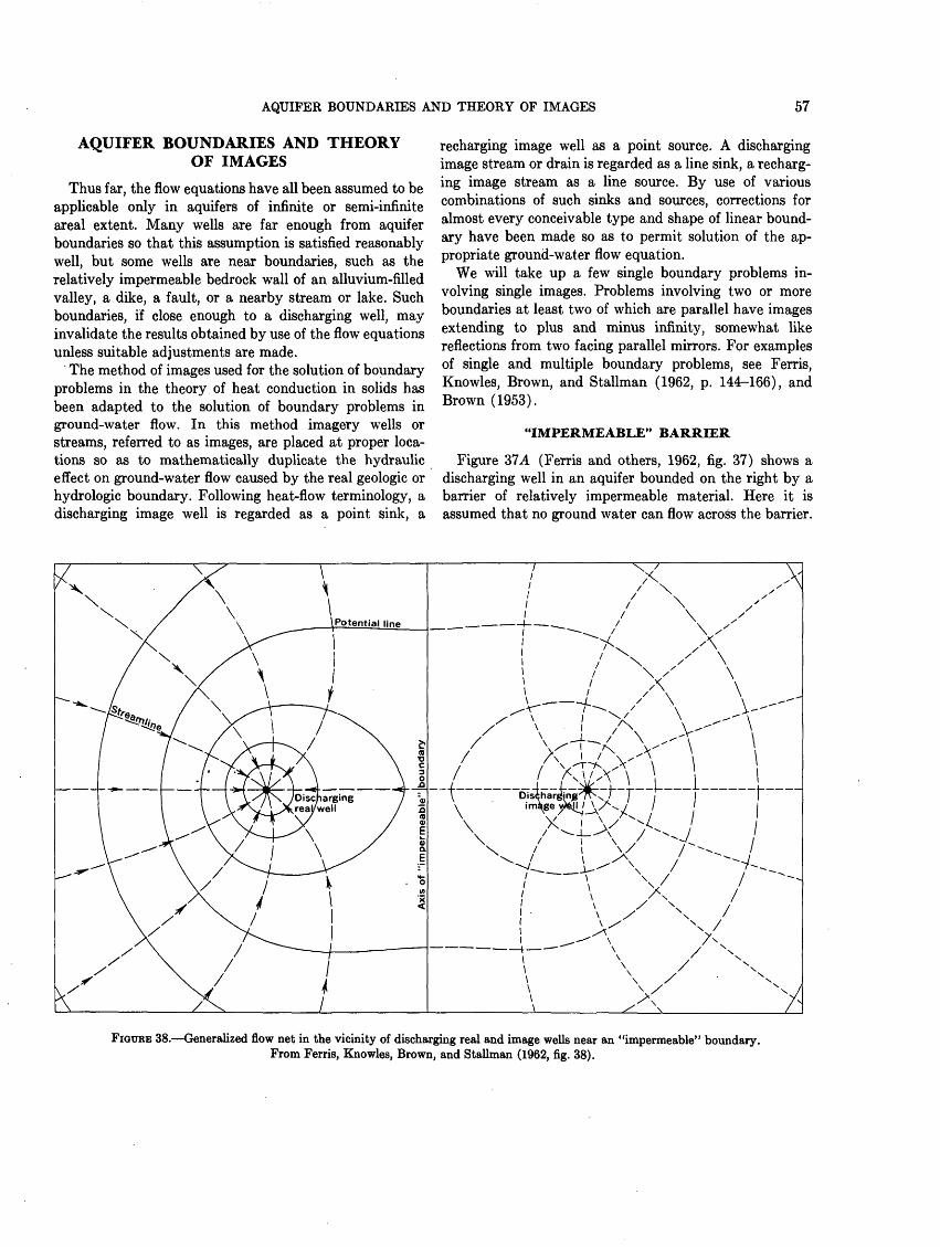
AQUIFER BOUNDARIES AND THEORY OF IMAGES 57
AQUIFER BOUNDARIES AND THEORY OF IMAGES
Thus far, the flow equations have all been assumed to be applicable only in aquifers of infinite or semi-infinite areal extent. Many wells are far enough from aquifer boundaries so that this assumption is satisfied reasonably well, but some wells are near boundaries, such as the relatively impermeable bedrock wall of an alluvium-filled valley, a dike, a fault, or a nearby stream or lake. Such boundaries, if close enough to a discharging well, may invalidate the results obtained by use of the flow equations unless suitable adjustments are made.
The method of images used for the solution of boundary problems in the theory of heat conduction in solids has been adapted to the solution of boundary problems in ground-water flow. In this method imagery wells or streams, referred to as images, are placed at proper loca tions so as to mathematically duplicate the hydraulic effect on ground-water flow caused by the real geologic or hydrologic boundary. Following heat-flow terminology, a discharging image well is regarded as a point sink, a
recharging image well as a point source. A discharging image stream or drain is regarded as a line sink, a recharg ing image stream as a line source. By use of various combinations of such sinks and sources, corrections for almost every conceivable type and shape of linear bound ary have been made so as to permit solution of the ap propriate ground-water flow equation.
We will take up a few single boundary problems in volving single images. Problems involving two or more boundaries at least two of which are parallel have images extending to plus and minus infinity, somewhat like reflections from two facing parallel mirrors. For examples of single and multiple boundary problems, see Ferris, Knowles, Brown, and Stallman (1962, p. 144-166), and Brown (1953).
"IMPERMEABLE" BARRIER
Figure 37'A (Ferris and others, 1962, fig. 37) shows a discharging well in an aquifer bounded on the right by a barrier of relatively impermeable material. Here it is assumed that no ground water can flow across the barrier.
\__/__4'__/\|£3_\ -I 1 L -
T Dis$harifn«77Tv>> T Til I
FIGURE 38. Generalized flow net in the vicinity of discharging real and image wells near an "impermeable" boundary.From Ferris, Knowles, Brown, and Stallman (1962, fig. 38).

58 GROUND-WATER HYDRAULICS
Data plot' ^^Theoretical straight-line plot
IQ-* 10-* io-3t/r*. IN DAY PER SQUARE FOOT
FIGURE 39. Effect of "impermeable" barrier on semilogarithmic plot of « versus t/r*.
10-2
The image system in the hydraulic counterpart of figure 37A, which permits a solution of the real problem by use of the flow equations, is shown in figure 37#. Here in an assumed infinite aquifer an image well having a discharge equal to that of the real well is placed the same distance (a)from the now imaginary barrier. The dashed theoretical cones of depression of the real and image wells intersect to form a ground-water divide at the hydraulic barrier, across which no flow can take place, thus satisfying the hydraulic conditions along the barrier. The resultant real cone of depression (heavy line) is the algebraic sum of the theoretical cones of depression (dashed lines) of the real and image wells. Figure 38 depicts the flow net of the two- well system. If the image well and image flow net are removed, the flow net on the left represents the effect of the "impermeable" boundary upon the discharging well.
If the drawdown (s) in an observation well near the real
well shown in figures 37 and 38 were plotted against t or t/r* on semilogarithmic paper, the curve would deviate downward from the theoretical straight-line plot as shown in figure 39. This shows that the effect of the barrier began to be felt at t/r*= about 1.8X10~4 day ft-2 and that the full effect was apparent at 0-2 = about 7.4 X10"4 day ft~2 . After the full effect was apparent, the slope of the lower straight line was two times the slope of the theoretical straight line, indicating an apparent transmissivity that was half that of the true value.
LINE SOURCE AT CONSTANT HEAD- PERENNIAL STREAM
If a well in an unconfined aquifer near a large perennial stream hydraulically connected to the aquifer is pumped, obviously the cone of depression cannot extend beyond

AQUIFER BOUNDARIES AND THEORY OF IMAGES 59
Perennial/stream Land surface
}_f2" Ji/ll^.J ̂ ^.-U ^^^ ; ."?>Nonp"umping water' level'. '. '.
; ' ' '.'.' : '. '.'Aquifer. : '. " . '. '
ConfiningJH- E^material-
A. REAL SYSTEM
Zero drawdown boundary (af = a,- )«
Buildup componentof image well
Discharging Q real welk /
Recharging .image well
water__level! I _
NOTE: Aquifer thickness 6 should be very large compared to resultant drawdown near real well
B. HYDRAULIC COUNTERPART OF REAL SYSTEM
FIGURE 40. Idealized section views of a discharging well in an aquifer bounded by a perennial stream and of the equivalent hydraulic system in an infinite aquifer. From Ferris, Knowles, Brown, and Stallman (1962, fig. 35).
the stream as the water level in such a stream remains relatively constant, assuming that the well discharge is small relative to the stream discharge. Such a situation is shown in figure 40A, in which the nearly straight, partly penetrating perennial stream is shown to be straight and fully penetrating and, hence, is equivalent to a line source at constant head.
The hydraulic counterpart in an assumed infinite aquifer is shown in figure 4QB, where a recharging image well, or point source, has been placed on a line connecting the real and image wells at right angles to the stream, at the same distance, o, from the stream. The recharge and discharge rates, Q, are assumed equal. The resulting cone of depres sion (heavy solid line), which is the algebraic sum of the dashed cones of depression of the real and image wells, intersects the level of the stream, as it should. The flow net for these conditions is shown in figure 41. Note that if the image well and its flow net are removed, the flow net on the left is that of the real well obtaining water by induced infiltration from the stream.
If the drawdown (s) in an observation well near the real well shown in figures 40 and 41 were plotted against t or
t/r2 on semilogarithmic paper, the curve would deviate upward from the theoretical straight-line plot as shown in figure 42. This shows that the effect of the stream began to be felt at t/r2 = about 2.8 X lO"4 day ft~2 and that the full effect was apparent at t/r* = about 3.5X10"3 day ft~2 . After the full effect was apparent, the slope of the upper straight line became horizontal, indicating an apparent infinite transmissivity.
One of the first applications of the image-well theory to ground-water flow was made by Theis (1941), who developed an equation and presented a graph for computing the percentage of the water pumped from a well near a stream that is diverted from the stream at a known dis tance from the well. (See also Glover and Balmer, 1954; Jenkins, 1968a, 1968b; Theis, 1963b; and Theis and Conover, 1963.)
APPLICATION OF IMAGE THEORY
It was evident in figure 39 that, for a discharging well in an aquifer bounded by a relatively impermeable barrier, a drawdown-time plot for an observation well near the pumped well was steepened (greater drawdown) at the value of t after the cone of depression reached the barrier, and that in figure 42, the converse was true. However, figures 39 and 42 are hypothetical straight-line curves; hence, they would hold true only when w<0.01. For largervalues of u, as for small values of t, large values of r, or for most unconfined aquifers, it is necessary to plot drawdown- time curves on logarithmic paper for comparison with the Theis curve (fig. 14), for which occur similar but curvi linear deviations from the theoretical curves. Computation of T and S by the usual curve-matching procedure would then be valid only for the early data before the boundary effects changed the slope of the curve. This would offer no problem for most confined aquifers, but in an unconfined aquifer sufficient time might not have elapsed to allow for reasonably complete drainage from storage.
Ferris, Knowles, Brown, and Stallman (1962, p. 161- 164) described a method of plotting s versus t or r2/t for matching with the Theis curve (fig. 14) that permits solving for T and S and also for the distance from the discharging well to the image well, which of course is at twice the distance to the actual boundary. If the boundary is concealed, as a hidden fault, three or more observation wells are required to locate the boundary. (See Ferris and others, 1962, p. 164-166; Moulder, 1963.)
A similar but much simpler method for the solution of single-boundary problems involving either a source or a sink was devised by Stallman (1963b). From figures 37 and 40, it is evident that ii s0 is the drawdown in an observation well, and sn and at arp^f.hft ftnmj>nnflnts of th^t drawrinvn caused, respectively, by the pumped (reaD well and by the discharging or recharging image well, then s0 is the alge-
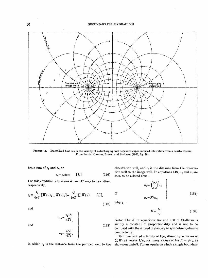
60 GROUND-WATER HYDRAULICS
FIGURE 41. Generalized flow net in the vicinity of a discharging well dependent upon induced infiltration from a nearby stream.From Ferris, Knowles, Brown, and Stallman (1962, fig. 36).
arebraic sum of sp and s t , or observation well, and rt is the distance from the observa-
_ tion well to the image well. In equations 148, up and w, S O = SP ±S> [LJ. (146) Seen to be related thus:
For this condition, equations 46 and 47 may be rewritten, /r-Vrpsnpnt.ivplv Wj = I J U>
\rp/
; WM ELI orrespectively,
(149)
(147) where
and
w« =
(150)
Note: The K in equations 149 and 150 of Stallman is ancj . (148) SUT1Ply a constant of proportionality and is not to be
confused with the K used previously to symbolize hydraulicconductivity.
Stallman plotted a family of logarithmic type curves of2] W(u} versus l/up for many values of his K=ri/rp, as
in which rp is the distance from the pumped well to the shown on plate 9. For an aquifer in which a single boundary
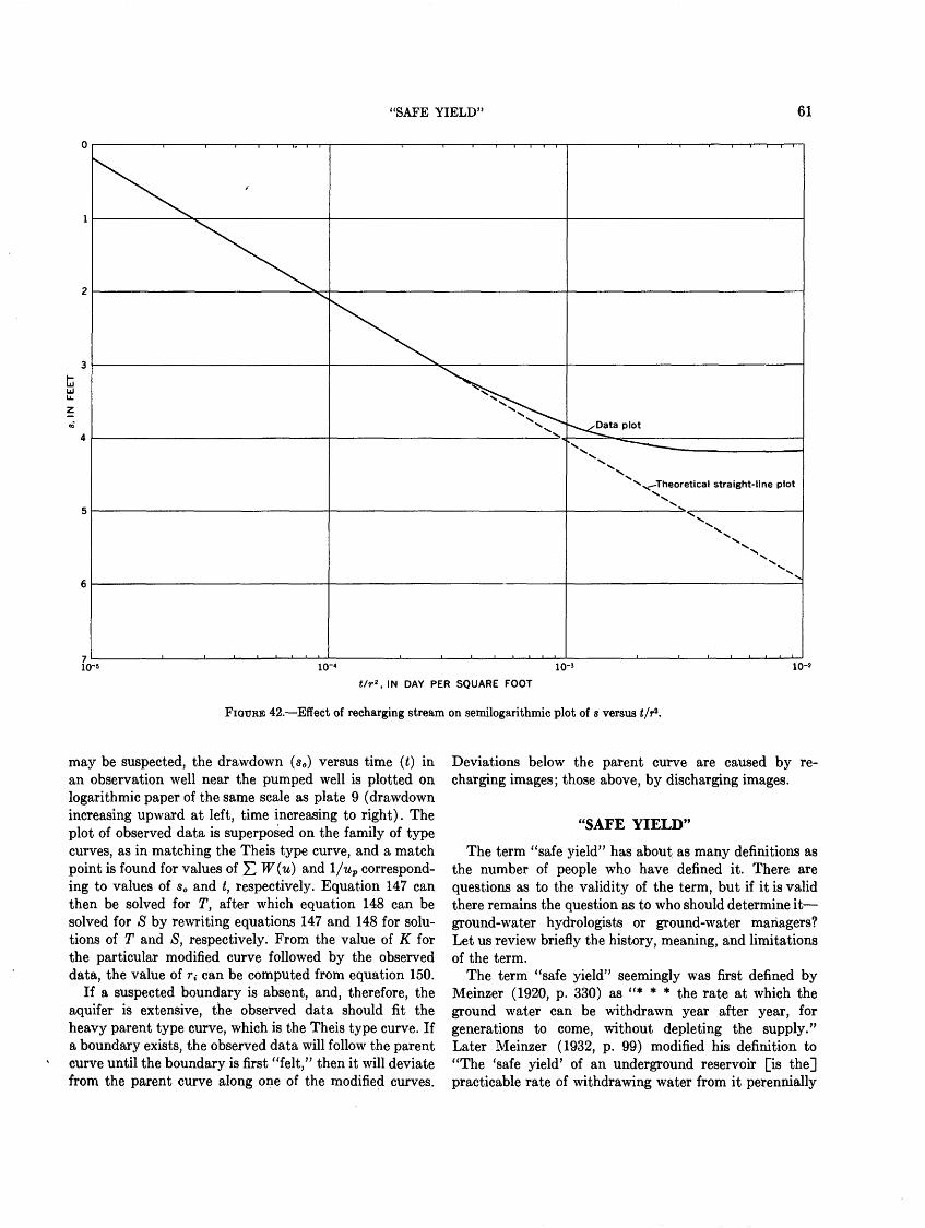
'SAFE YIELD' 61
'Data plot
. Theoretical straight-line plot
io-« io-3t/r2 , IN DAY PER SQUARE FOOT
FIGURE 42. Effect of recharging stream on semilogarithmic plot of s versus t/r*.
may be suspected, the drawdown (sc ) versus time (0 in an observation well near the pumped well is plotted on logarithmic paper of the same scale as plate 9 (drawdown increasing upward at left, time increasing to right). The plot of observed data is superposed on the family of type curves, as in matching the Theis type curve, and a match point is found for values of £ W(u) and l/up correspond ing to values of sc and t, respectively. Equation 147 can then be solved for T, after which equation 148 can be solved for S by rewriting equations 147 and 148 for solu tions of T and S, respectively. From the value of K for the particular modified curve followed by the observed data, the value of r, can be computed from equation 150.
If a suspected boundary is absent, and, therefore, the aquifer is extensive, the observed data should fit the heavy parent type curve, which is the Theis type curve. If a boundary exists, the observed data will follow the parent curve until the boundary is first "felt," then it will deviate from the parent curve along one of the modified curves.
Deviations below the parent curve are caused by re charging images; those above, by discharging images.
"SAFE YIELD"
The term "safe yield" has about, as many definitions as the number of people who have defined it. There are questions as to the validity of the term, but if it is valid there remains the question as to who should determine it ground-water hydrologists or ground-water managers? Let us review briefly the history, meaning, and limitations of the term.
The term "safe yield" seemingly was first defined by Meinzer (1920, p. 330) as "* * * the rate at which the ground water can be withdrawn year after year, for generations to come, without depleting the supply." Later Meinzer (1932, p. 99) modified his definition to "The 'safe yield' of an underground reservoir [is the^ practicable rate of withdrawing water from it perennially
62 GROUND-WATER HYDRAULICS
for human use * * *." Although there was nothing wrong with Meinzer's early definitions, they seemingly did not wholly satisfy all ground-water hydrologists, for beginning about 20 years later many began redefining the concept in more and more precise terms to suit themselves or to suit the particular ground-water conditions with which they were concerned. For a r&ume' of many of these definitions, see Kazmann (1951, 1956), Hantush (1955, p. 71), and Todd (1959, p. 200-218).
As stated by Kazmann (1956, p. 1103-2), "The thought became current that the 'safe yield' of an aquifer was surely determinable in advance of ground-water develop ment or even after development had begun." I might add that the thought also became current that one could put a number on the safe yield of a ground-water reservoir regardless of its method of development. However, as stated by Thomas (1951, p. 262):
In a ground-water reservoir where the water is unconfined in certain areas (recharge areas) and under artesian pressure in other places, the safe yield will be a certain quantity if it is specified that all withdrawals must be by flow from artesian wells, a larger quantity if it is permissible to pump water from depths as great as 50 feet, and still more if allowable pumping lifts are as much as 500 feet. But the safe yield will vary also depending upon the locations of wells and the type of wells constructed. Assuming that the well construction and spacing of individual wells are suitable for maxi mum recovery of water, the safe yield will be a certain quantity if all wells are 40 miles from the recharge area, considerably greater if they are about 10 miles away, and still more if they are adjacent to or within the recharge area.
The multiplicity and looseness of definitions led Kaz mann to title his 1956 paper " 'Safe Yield' in Ground- Water Development, Reality or Illusion?," and led Thomas (1951, p. 261) to say: " 'Safe yield.' This term, originated by hydrologists, may well prove awkward for them because of the variety of interpretations possible. 'Safe yield' is an Alice-in-Wonderland term which means whatever its user chooses."
I have a definition which I taught at U.S. Geological Survey Ground Water Short Courses beginning in 1952, namely, "The amount of ground water one can withdraw without getting into trouble." "Withdraw" may mean from flowing or pumped wells, and it may mean con tinuously, as for many industrial or municipal supplies, or seasonally, as for irrigation. "Trouble" may mean any thing under the sun; such as (1) running out of water,(2) drawing in salt water, or other undesirable water,(3) getting shot, or shot at, by an irate nearby wellowner or landowner, (4) getting sued by a less irate neighbor, or (5) getting sued for depleting the flow of a nearby stream for which the water rights have been appropriated. My definition may sound facetious to some, but remembering that I would not attempt to put a number on it before development or in the early stages of development, espe
cially if I did not know where and how the withdrawal would be made, it actually makes more sense than many definitions, does not differ significantly from Meinzer's original definitions, and is very close to the later definition of Todd (1959, p. 200): "The safe yield of a ground water basin is the amount of water which can be withdrawn from it annually without producing an undesired result."
To determine whether or not a desired quantity and quality of water can be withdrawn from a given ground- water reservoir generally requires an adequate knowledge of the geologic framework and its plumbing system plus the application of philosophy, common sense, and knowl edge of the proposed type of development that owners or managers have in mind. As problems become more and more complex, however, such as those involving large investments in land and wells, withdrawal of water from both streams and wells that tap a common source, or conflicts in water rights, then the solution may require highly detailed study. The modern approach is for the hydrologist to acquire sufficient detail concerning the combined ground- and surface-water system so aquifer response can be predicted by electric-analog or mathe matical models. Then management, such as state or local water-conservation agencies, within the framework of prevailing laws or regulations, may test the response of the system to various assumed stresses and thereby select the most desirable or equitable distribution of available water. Thus the role of the hydrologist is to gather and present the facts; the water manager determines who shall have how much water and from what source. In so doing, the manager generally requires and obtains considerable con tinuing assistance from the hydrologist. (See Wood and Gabrysch, 1965; Walton and Prickett, 1963; Moore and Wood, 1967.)
In the sections that follow, some additional references will be made to safe yield in discussing examples of different types of ground-water reservoirs.
THE SOURCE OF WATER DERIVED FROM WELLS
Under the above title Theis (1940) stated concisely the hydrologic principles upon which depend much of our present quantitative approach to ground-water problems. The statements that follow are summarized from these principles.
The essential factors that determine the response of aquifers to development by wells are:
1. Distance to, and character of, the recharge.2. Distance to the locality of natural discharge.3. Character of the cone of depression in the aquifer,
which depends upon the values of T (which contains K and 6) and S.

THE SOURCE OF WATER DERIVED FROM WELLS 63
Prior to development by wells, aquifers are in a state of dynamic equilibrium, in that over long periods of time recharge and discharge virtually balance. Discharge from wells upsets this balance by producing a loss from storage, and a new state of dynamic equilibrium cannot be reached until there is no further loss from storage. This can only be accomplished by:
1. Increase in recharge (natural or artificial).2. Decrease in natural discharge.3. A combination of 1 and 2.
The above statements were put into equation form with terms having the dimensions LST~1 by Hilton H. Cooper, Jr., U.S. Geological Survey (written commun., April 1967). I have added the A/i/At and have assigned to the terms the dimensions LT~l as follows:
A/i At
(151)
where
R = recharge rate per unit area,A/2 = change in recharge rate per unit area,D = natural discharge rate per unit area,AZ) = change in discharge rate per unit area,<7 = rate of withdrawal from wells per unit area, and
A/iS =rate of change in storage per unit area.
At
Assuming that additions to the aquifer (left-hand terms in eq. 151) are positive, that withdrawals from the aquifer (right-hand terms in eq. 151) are negative, and that over the years RttD, then solving equation 151 for q, we obtain
] (152)- (-AD) - -S
If dynamic equilibrium can be reestablished, there will
A/ibe no further withdrawals from storage, so that S »0,
At
and equation 152 becomes[L77-1]. (153)
We will see in the last section that equation 153 is applic able only to certain types of aquifer systems. For aquifers in which a new dynamic equilibrium is not attainable, continued withdrawal from storage may be greater than changes in recharge or discharge rates, and storage may be the principal or sole source of water. Under such conditions equation 152, or a part of it, is applicable. If we wish to know the total volumes of water involved, each term in equations 152 or 153 must be multiplied by the area (A) over which the changes occur.
Before taking up examples of different types of aquifers, let us review the following summary statements by Theis (1940, p. 280), which are important enough to quote completely:
1. All water discharged by wells is balanced by a loss of water somewhere.
2. This loss is always to some extent and in many cases largely from storage in the aquifer. Some ground water is always mined. The reservoir from which the water is taken is in effect bounded by time and by the structure of the aquifer as well as by material boundaries. The amount of water re moved from any area is proportional to the drawdown, which in turn is proportional to the rate of pumping. Therefore, too great concentration of pumping in any area is to be discouraged and a uniform areal distribution of development over the area where the water is shallow should be encouraged, so far as is consistent with soil and marketing or other economic conditions.
3. After sufficient time has elapsed for the cone to reach the area of recharge, further discharge by wells will be made up at least in part by an increase in the recharge if previously there has been rejected recharge. If the recharge was previously re jected through transpiration from nonbeneficial vegetation, no economic loss is suffered. If the recharge was rejected through springs or refusal of the aquifer to absorb surface waters, rights to these surface waters may be injured.
4. Again, after sufficient time has elapsed for the cone to reach the areas of natural discharge, further discharge by wells will be made up in part by a diminution in the natural discharge. If this natural discharge fed surface streams, prior rights to the surface water may be injured.
5. In most artesian aquifers excluding very extensive ones, such as the Dakota sandstone little of the water is taken from storage. In these aquifers, because the cones of depression spread with great rapidity, each well in a short time has its maximum effect on the whole aquifer and obtains most of its water by increase of recharge or decrease of natural discharge. Such an artesian basin can be treated as a unit, as is done in the New Mexico ground-water law, and the laws of some other Western States that follow this law. In large nonartesian aquifers, where pumping is done at great distances from the localities of intake or outlet, however, the effects of each well are for a considerable time confined to a rather small radius and the water is taken from storage in the vicinity of the well. Hence these large ground-water bodies cannot be considered a unit in utilizing the ground water. Proper conservation measures will consider such large aquifers to be made up of smaller units, and will attempt to limit the development in each unit. Such procedure would also be advisable, although not as necessary, in an artesian aquifer.
6. The ideal development of any aquifer from the standpoint of the maximum utilization of the supply would follow these points:(a) The pumps should be placed as close as economically pos
sible to areas of rejected recharge or natural discharge where ground water is being lost by evaporation or transpiration by nonproductive vegetation, or where the surface water fed by, or rejected by, the ground water cannot be used. By so doing this lost water would be utilized by the pumps with a minimum lowering of the water level in the aquifer.
(b) In areas remote from zones of natural discharge or re jected recharge, the pumps should be spaced as uni formly as possible throughout the .available area. By so
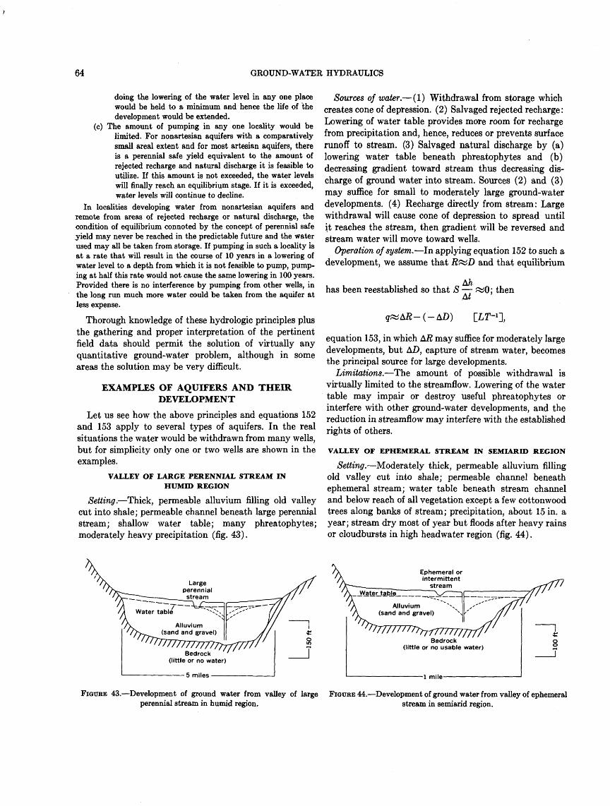
64 GROUND-WATER HYDRAULICS
doing the lowering of the water level in any one place would be held to a minimum and hence the life of the development would be extended.
(c) The amount of pumping in any one locality would be limited. For nonartesian aquifers with a comparatively small areal extent and for most artesian aquifers, there is a perennial safe yield equivalent to the amount of rejected recharge and natural discharge it is feasible to utilize. If this amount is not exceeded, the water levels will finally reach an equilibrium stage. If it is exceeded, water levels will continue to decline.
In localities developing water from nonartesian aquifers and remote from areas of rejected recharge or natural discharge, the condition of equilibrium connoted by the concept of perennial safe yield may never be reached in the predictable future and the water used may all be taken from storage. If pumping in such a locality is at a rate that will result in the course of 10 years in a lowering of water level to a depth from which it is not feasible to pump, pump ing at half this rate would not cause the same lowering in 100 years. Provided there is no interference by pumping from other wells, in the long run much more water could be taken from the aquifer at less expense.
Thorough knowledge of these hydrologic principles plus the gathering and proper interpretation of the pertinent field data should permit the solution of virtually any quantitative ground-water problem, although in some areas the solution may be very difficult.
EXAMPLES OF AQUIFERS AND THEIR DEVELOPMENT
Let us see how the above principles and equations 152 and 153 apply to several types of aquifers. In the real situations the water would be withdrawn from many wells, but for simplicity only one or two wells are shown in the examples.
VALLEY OF LARGE PERENNIAL STREAM IN HUMID REGION
Setting. Thick, permeable alluvium filling old valley cut into shale; permeable channel beneath large perennial stream; shallow water table; many phreatophytes; moderately heavy precipitation (fig. 43).
Sources of water. (1) Withdrawal from storage which creates cone of depression. (2) Salvaged rejected recharge: Lowering of water table provides more room for recharge from precipitation and, hence, reduces or prevents surface runoff to stream. (3) Salvaged natural discharge by (a) lowering water table beneath phreatophytes and (b) decreasing gradient toward stream thus decreasing dis charge of ground water into stream. Sources (2) and (3) may suffice for small to moderately large ground-water developments. (4) Recharge directly from stream: Large withdrawal will cause cone of depression to spread until it reaches the stream, then gradient will be reversed and stream water will move toward wells.
Operation of system. In applying equation 152 to such a development, we assume that RttD and that equilibrium
Ah has been reestablished so that S £^0; then
equation 153, in which A/2 may suffice for moderately large developments, but AD, capture of stream water, becomes the principal source for large developments.
Limitations. The amount of possible withdrawal is virtually limited to the streamflow. Lowering of the water table may impair or destroy useful phreatophytes or interfere with other ground-water developments, and the reduction in streamflow may interfere with the established rights of others.
VALLEY OF EPHEMERAL STREAM IN SEMIARID REGION
Setting. Moderately thick, permeable alluvium filling old valley cut into shale; permeable channel beneath ephemeral stream; water table beneath stream channel and below reach of all vegetation except a few cottonwood trees along banks of stream; precipitation, about 15 in. a year; stream dry most of year but floods after heavy rains or cloudbursts in high headwater region (fig. 44) .
Largeperennial
stream
Ephemeral or intermittent
stream
Alluvium (sand and gravel)
17777777777Bedrock
(little or no water)
5 miles
Bedrock (little or no usable water)
1 mile-
FIGURE 43. Development of ground water from valley of large perennial stream in humid region.
FIGURE 44. Development of ground water from valley of ephemeral stream in semiarid region.
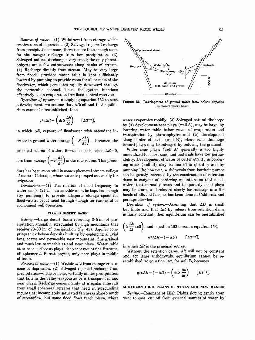
65
Sources of water. (1) Withdrawal from storage which creates cone of depression. (2) Salvaged rejected recharge from precipitation none; there is more than enough room for the meager recharge from low precipitation. (3) Salvaged natural discharge very small; the only phreat- ophytes are a few cottonwoods along banks of stream. (4) Recharge directly from stream: May be very large from floods, provided water table is kept sufficiently lowered by pumping to provide room for all or most of the floodwater, which percolates rapidly downward through the permeable channel. Thus, the system functions effectively as an evaporation-free flood-control reservoir.
Operation of system. In applying equation 152 to such a development, we assume that AZ)£bO and that equilib rium cannot be reestablished; then
in which A/2, capture of floodwater with attendant in
crease in ground-water storage (+S ] , becomes the\ ^" /
principal source of water. Bewteen floods, when AR=0,
loss from storage ( S I is the sole source. This proce
dure has been successful in some ephemeral stream valleys of eastern Colorado, where water is pumped seasonally for irrigation.
Limitations. (1) The relation of flood frequency to water needs. (2) The water table must be kept low enough (by pumping) to provide adequate storage space for floodwaters, yet it must be high enough for successful or economical well operation.
CLOSED DESERT BASIN
Setting. Large desert basin receiving 3-5 in. of pre cipitation annually, surrounded by high mountains that receive 20-30 in. of precipitation (fig. 45). Aquifer com prises thick bolson deposits built up by coalescing alluvial fans, coarse and permeable near mountains, fine grained and much less permeable at and near playa. Water table at or near surface at playa, deep near mountains. Streams, all ephemeral. Phreatophytes, only near playa in middle of basin.
Sources of water. (1) Withdrawal from storage creates cone of depression. (2) Salvaged rejected recharge from precipitation little or none; virtually all the precipitation that falls in the valley evaporates or is transpired in and near playa. Recharge comes mainly at irregular intervals from small ephemeral streams that head in surrounding mountains; incompletely saturated fan areas absorb much of streamflow, but some flood flows reach playa, where
Alluvium (silt, sand, and gravel)
20 miles
FIGURE 45. Development of ground water from bolson deposits in closed desert basin.
water evaporates rapidly. (3) Salvaged natural discharge by (a) development near playa (well A) , may be large, by lowering water table below reach of evaporation and transpiration by phreatophytes and (b) development along border of basin (well B), where some discharge toward playa may be salvaged by reducing the gradient.
Water near playa (well A) generally is too highly mineralized for most uses, and materials have low perme ability. Development of water of better quality in border ing areas (well B) may be limited in quantity and bypumping lift; however, withdrawals from bordering areas can be greatly increased by the construction of retention dams in canyons of bordering mountains so that flood- waters that normally reach and temporarily flood playa may be stored and released slowly for recharge into the heads of alluvial fans, as has been done in California and perhaps elsewhere.
Operation of system. Assuming that AD is small but finite and that AR by release from retention dams is fairly constant, then equilibrium can be reestablished
S £^0 ) , A< /
and equation 152 becomes equation 153,
in which AT? is the principal source.Without the retention dams, AK will not be constant
and, for large withdrawals, equilibrium cannot be re established, so equation 152, for well B, becomes
- (±S [L77-1].
SOUTHERN HIGH PLAINS OF TEXAS AND NEW MEXICO
Setting. Remnant of High Plains sloping gently from west to east, cut off from external sources of water by
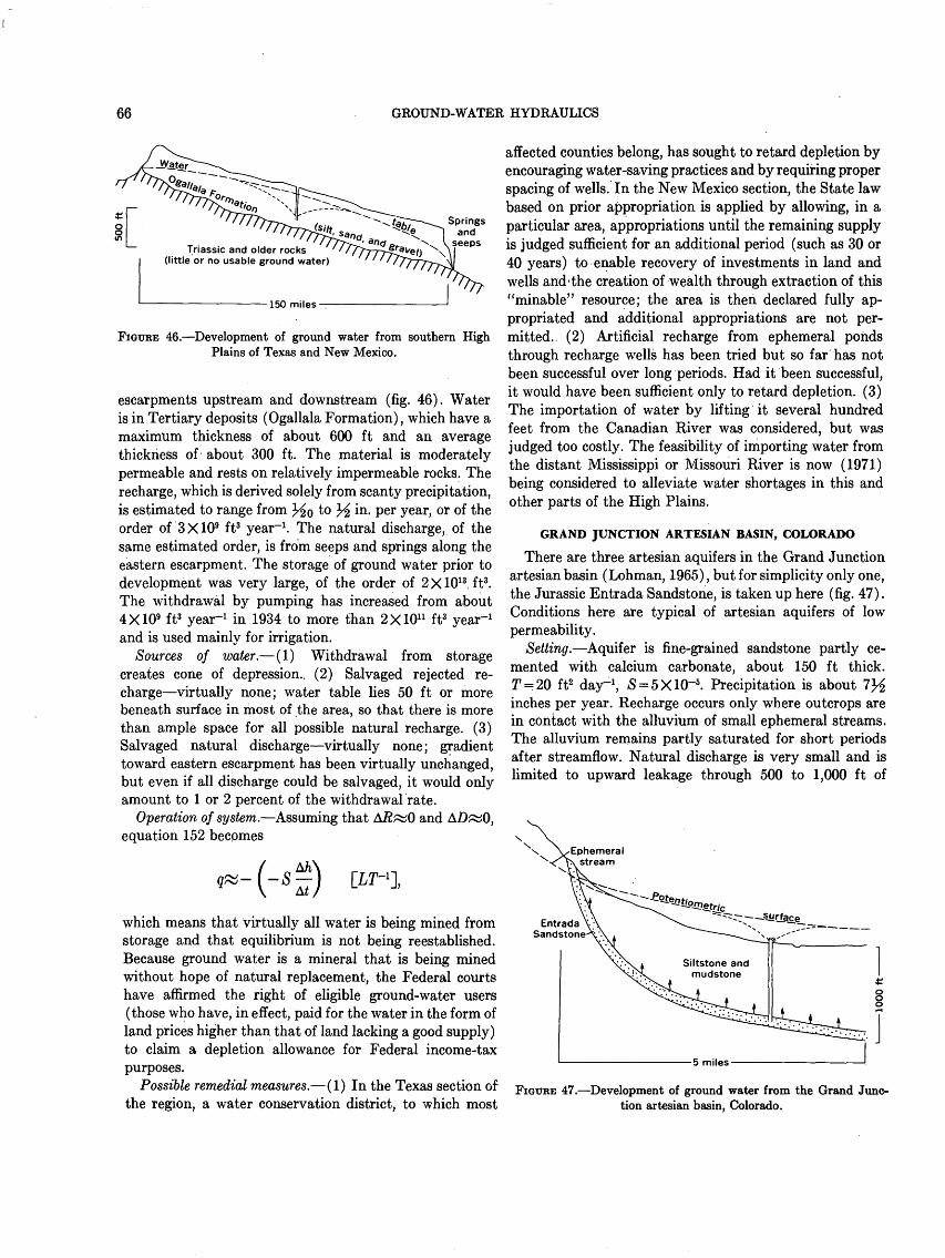
66 GROUND-WATER HYDRAULICS
Triassic and older rocks (little or no usable ground water)
-150 miles
FIGURE 46. Development of ground water from southern High Plains of Texas and New Mexico.
escarpments upstream and downstream (fig. 46). Water is in Tertiary deposits (Ogallala Formation), which have a maximum thickness of about 600 ft and an average thickness of about 300 ft. The material is moderately permeable and rests on relatively impermeable rocks. The recharge, which is derived solely from scanty precipitation, is estimated to range from %Q to % in. per year, or of the order of 3X109 ft3 year"1 . The natural discharge,, of the same estimated order, is from seeps and springs along the eastern escarpment. The storage of ground water prior to development was very large, of the order of 2 X10¹³ , ft3 . The withdrawal by pumping has increased from about 4X109 ft3 year-1 in 1934 to more than 2X1011 ft3 year-1 and is used mainly for irrigation.
Sources of water. (1) Withdrawal from storage creates cone of depression.. (2) Salvaged rejected re charge virtually none; water table lies 50 ft or more beneath surface in most of the area, so that there is more than ample space for all possible natural recharge. (3) Salvaged natural discharge virtually none; gradient toward eastern escarpment has been virtually unchanged, but even if all discharge could be salvaged, it would only amount to 1 or 2 percent of the withdrawal rate.
Operation of system. Assuming that A/?^0 and AD«0, equation 152 becomes
A/i\
M)
which means that virtually all water is being mined from storage and that equilibrium is not being reestablished. Because ground water is a mineral that is being mined without hope of natural replacement, the Federal courts have affirmed the right of eligible ground-water users (those who have, in effect, paid for the water in the form of land prices higher than that of land lacking a good supply) to claim a depletion allowance for Federal income-tax purposes.
Possible remedial measures. (1) In the Texas section of the region, a water conservation district, to which most
affected counties belong, has sought to retard depletion by encouraging water-saving practices and by requiring proper spacing of wells. In the New Mexico section, the State law based on prior appropriation is applied by allowing, in a particular area, appropriations until the remaining supply is judged sufficient for an additional period (such as 30 or 40 years) to enable recovery of investments in land and wells and'the creation of wealth through extraction of this "minable" resource; the area is then declared fully ap propriated and additional appropriations are not per mitted. (2) Artificial recharge from ephemeral ponds through recharge wells has been tried but so far has not been successful over long periods. Had it been successful, it would have been sufficient only to retard depletion. (3) The importation of water by lifting it several hundred feet from the Canadian River was considered, but was judged too costly. The feasibility of importing water from the distant Mississippi or Missouri River is now (1971) being considered to alleviate water shortages in this and other parts of the High Plains.
GRAND JUNCTION ARTESIAN BASIN, COLORADO
There are three artesian aquifers in the Grand Junction artesian basin (Lohman, 1965), but for simplicity only one, the Jurassic Entrada Sandstone, is taken up here (fig. 47). Conditions here are typical of artesian aquifers of low permeability.
Setting. Aquifer is fine-grained sandstone partly ce mented with calcium carbonate, about 150 ft thick. T = 20 ft2 day-1 , S = 5X1Q-5 . Precipitation is about 7^ inches per year. Recharge occurs only where outcrops are in contact with the alluvium of small ephemeral streams. The alluvium remains partly saturated for short periods after streamflow. Natural discharge is very small and is limited to upward leakage through 500 to 1,000 ft of
5 miles-
FIGURE 47. Development of ground water from the Grand Junc tion artesian basin, Colorado.
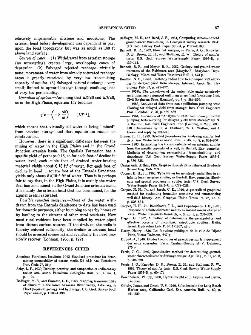
REFERENCES CITED 67
relatively impermeable siltstone and mudstone. The artesian head before development was dependent in part upon the local topography but was as much as 160 ft above land surface.
Sources of water. (1) Withdrawal from artesian storage (no unwatering) creates large, overlapping cones of depression. (2) Salvaged rejected recharge virtually none; movement of water from already saturated recharge areas is greatly restricted by very low transmitting capacity of aquifer. (3) Salvaged natural discharge very small; limited to upward leakage through confining beds of very low permeability.
Operation of system. Assuming that A/E^O and AD^O, as in the High Plains, equation 152 becomes
[LIT'],
which means that virtually all water is being "mined" from artesian storage and that equilibrium cannot be reestablished.
However, there is a significant difference between the mining of water in the High Plains and in the Grand Junction artesian basin. The Ogallala Formation has a specific yield of perhaps 0.15, so for each foot of decline in water level, each cubic foot of drained water-bearing material yields about 0.15 ft3 of water. For each foot of decline in head, 1 square foot of the Entrada Sandstone yields only about 5 X 10~5 ft3 of water. Thus it is perhaps fair to say that, in the High Plains, it is mainly the water that has been mined; in the Grand Junction artesian basin, it is mainly the artesian head that has been mined, for the aquifer is still saturated.
Possible remedial measures. Most of the water with drawn from the Entrada Sandstone to date has been used for domestic purposes, either by piping to nearby homes or by hauling to the cisterns of other rural residents. Now most rural residents have been supplied by water piped from distant surface sources. If the draft on the wells is thereby reduced sufficiently, the decline in artesian head should be arrested somewhat and eventually the head may slowly recover (Lohman, 1965, p. 122).
REFERENCES CITED
American Petroleum Institute, 1942, Standard procedure for deter mining permeability of porous media [2d ed.]: Am. Petroleum Inst. Code 27, 21 p.
Athy, L. F., 1930, Density, porosity, and compaction of sedimentary rocks: Am. Assoc. Petroleum Geologists Bull., v. 14, no. 1, p. 1-24.
Bedinger, M. S., and Emmett, L. F., 1963, Mapping transmissibility of alluvium in the lower Arkansas River valley, Arkansas, in Short papers in geology and hydrology: U.S. Geol. Survey Prof. Paper 475-C, p. C188-C190.
Bedinger, M. S., and Reed, J. E., 1964, Computing stream-induced ground-water fluctuation, in Geological survey research 1964: U.S. Geol. Survey Prof. Paper 501-B, p. B177-B180.
Bennett, R. R., 1962, Flow net analysis, in Ferris, J. G., Knowles, . D. B., Brown, R. H., and Stallman, R. W., Theory of aquifer tests: U.S. Geol. Survey Water-Supply Paper 1536-E, p. 139-144.
Bennett, R. R., and Meyer, R. R., 1952, Geology and ground-water resources of the Baltimore area [Maryland]: Maryland Dept. Geology, Mines and Water Resources Bull. 4, 573 p.
Boulton, N. S., 1954a, Unsteady radial flow to a pumped well allow ing for delayed yield from storage: Internat. Assoc. Sci. Hy drology Pub. 37, p. 472-477.
1954b, The drawdown of the water table under nonsteady conditions near a pumped well in an unconfined formation: Inst. Civil Engineers Proc. [London], pt. 3, p. 564-579.
1963, Analysis of data from non-equilibrium pumping tests allowing for delayed yield from storage: Inst. Civil Engineers Proc. [London], v. 26, p. 469-482.
1964, Discussion of "Analysis of data from non-equilibriumpumping tests allowing for delayed yield from storage" by N. S. Boulton: Inst. Civil Engineers Proc. [London], v. 28, p. 603- 610. [Discussions by R. W. Stallman, W. C. Walton, and J. Ineson and reply by author.]
Brown, R. H., 1953, Selected procedures for analyzing aquifer test data: Am. Water Works Assoc. Jour., v. 45, no. 8, p. 844-866.
1963, Estimating the transmissibility of an artesian aquifer from the specific capacity of a well, in Bentall, Ray, compiler, Methods of determining permeability, transmissibility, and drawdown: U.S. Geol. Survey Water-Supply Paper 1536-1, p. 336-338.
Casagrande, Arthur, 1937, Seepage through dams: Harvard Graduate School Eng. Pub. 209.
Cooper, H. H., Jr., 1963, Type curves for nonsteady radial flow in an infinite leaky artesian aquifer, in Bentall, Ray, compiler, Short cuts and special problems in aquifer tests: U.S. Geol. Survey Water-Supply Paper 1545-C, p. C48-C55.
Cooper, H. H., Jr., and Jacob, C. E., 1946, A generalized graphical method for evaluating formation constants and summarizing well-field history: Am. Geophys. Union Trans., v. 27, no. 4, p. 526-534.
Cooper, H. H., Jr., Bredehoeft, J. D., and Papadopulos, I. S., 1967, Response of a finite-diameter well to an instantaneous charge of water: Water Resources Research, v. 3, no. 1, p. 263-269.
Dagan, G., 1967, A method of determining the permeability and effective porosity of unconfined anisotropic aquifers: Haifa, Israel, Hydraulics Lab. P. N. 1/1967, 49 p.
Darcy, Henry, 1856, Les fontaines publiques de la ville de Dijon: Paris, Victor Dalmont, 647 p.
Dupuit, J., 1848, Etudes theoriques et practiques sur le mouvement des eaux courantes: Paris, Carilian-Goeury et V. Dalmont, 275 p.
Ferris, J. G., 1950, Quantitative method for determining ground- water characteristics for drainage design: Agr. Eng., v. 31, no. 6, p. 285-291.
Ferris, J. G., Knowles, D. B., Brown, R. H., and Stallman, R. W., 1962, Theory of aquifer tests: U.S. Geol. Survey Water-Supply Paper 1536-E, p. 69-174.
Forchheimer, Philipp, 1930, Hydraulik [3d ed.]: Leipzig and Berlin, Teubner.
Gilluly, James, and Grant, U. S., 1949, Subsidence in the Long Beach Harbor area, California: Geol. Soc. America Bull., v. 60, p. 461-529.
68 GROUND-WATER HYDRAULICS
Glover, R. E., and Balmer, C. G., 1954, River depletion resultingfrom pumping a well near a river: Am. Geophys. Union Trans.,v. 35, p. 468-470.
Hagen, G. H. L., 1839, Ueber die Bewegung des Wassers in engencylindrischen Rohren: Annalen Physik u. Chemie [Leipzig],v. 36, p. 423-442.
Hantush, M. S., 1955, Preliminary quantitative study of the Roswellground-water reservoir, New Mexico: New Mexico Inst. Miningand Technology, 113 p.
1956, Analysis of data from pumping tests in leaky aquifers: Am. Geophys. Union Trans., v. 37, no. 6, p. 702-714.
1959, Nonsteady flow to flowing wells in leaky aquifer: Jour. Geophys. Research, v. 64, no. 8, p. 1043-1052.
1960, Modification of the theory of leaky aquifers: Jour.Geophys. Research, v. 65, no. 11, p. 3713-3725.
1961, Tables of the function H(fm e-«
u, /3)= / Jtt y
erfc New Mexico Inst. Mining and Tech-
nology, Prof. Paper 103, 14 p.1964, Hydraulics of wells, in Chow, Ven Te, ed., Advances in
hydroscience, volume 1: New York, Academic Press Inc., p. 281-442.
Hantush, M. S., and Jacob, C. E., 1954, Plane potential flow of ground water with linear leakage: Am. Geophys. Union Trans., v. 35, no. 6, p. 917-936.
1955, Nonsteady radial flow in an infinite leaky aquifer: Am. Geophys. Union Trans., v. 36, no. 1, p. 95-100.
Hedberg, H. D., 1936, Gravitational compaction of clays and shales: Am. Jour. Sci., v. 31, p. 241-287.
Hubbert, M. K., 1940, The theory of ground-water motion: Jour. Geology, v. 48, no. 8, pt. 1, p. 785-944.
Hurr, R. T., 1966, A new approach for estimating transmissibility from specific capacity: Water Resources Research, v. 2, no. 4,. p. 657-664.
Ingersol, R. I., Zobel, O. J., and Ingersol, A. C., 1954, Heat conduc tion, with engineering, geological, and other applications: Madison, Wisconsin Univ. Press, 325 p.
Jacob, C. E., 1940, On the flow of water in an elastic artesian aquifer: Am. Geophys. Union Trans., pt. 2, p. 574-586.
1943, Correlation of ground-water levels and precipitation in Long Island, New York: Am. Geophys. Union Trans., v. 24, pt. 2, p. 564-573.
1946, Radial flow in a leaky artesian aquifer: Am. Geophys. Union Trans., v. 27, no. 2, p. 198-205.
1947, Drawdown test to determine effective radius of ar tesian well: Am. Soc. Civil Engineers Trans., v. 112, p. 1047- 1070.
1963a, Determining the permeability of water-table aqui fers, in Bentall, Ray, compiler, Methods of determining perme ability, transmissibility, and drawdown: U.S. Geol. Survey Water-Supply Paper 1536-1, p. 245-271.
1963b, Correction of drawdowns caused by a pumped welltapping less than the full thickness of an aquifer, in Bentall, Ray, compiler, Methods of determining permeability, trans missibility, and drawdown: U.S. Geol. Survey Water-Supply Paper 1536-1, p. 272-292.
Jacob, C. E., and Lohman, S. W., 1952, Nonsteady flow to a well of constant drawdown in an extensive aquifer: Am. Geophys. Union Trans., v. 33, p. 559-569.
Jaeger, J. C., 1942, Heat conduction in a wedge, or an infinite cylinder whose cross section is a circle or sector of a circle: Philos. Mag., ser. 7, v. 33, no. 222, p. 527-536.
Jenkins, C. T., 1963, Graphical multiple-regression analysis of aquifer tests, in Short papers in geology and hydrology: U.S. Geol. Survey Prof. Paper 475-C, p. C198-C201.
1968a, Techniques for computing rate and volume of stream depletion by wells: Ground Water, v. 6, no. 2, p. 37-46.
1968b, Electric-analog and digital-computer model analysesof stream depletion by wells: Ground Water, v. 6, no. 6, p. 27-34.
Kazmann, R. G., 1951, The role of aquifers in water supply: Am. Geophys. Union Trans., v. 32, no. 2, p. 227-230.
1956, "Safe yield" in ground-water development, reality or illusion?: Am. Soc. Civil Engineers Proc., Irrig. Drainage Div. Jour., v. 82, no. IR3, p. 1103-1-1103-12.
Leggette, R. M., 1936, Ground water in northwestern Pennsylvania: Penna. Geol. Survey Bull. W-3, 215 p.
Lohman, S. W., 1936, Geology and ground-water resources of the Elizabeth City area, North Carolina: U.S. Geol. Survey Water- Supply Paper 773-A, 57 p.
1961, Compression of elastic artesian aquifers, in Short papers in the geologic and hydrologic sciences: U.S. Geol. Survey Prof. Paper 424-B, p. B47-B49.
1963, Method for determination of the coefficient of storage from-straight-line plots without extrapolation, in Bentall, Ray, compiler, Shortcuts and special problems in aquifer tests: U.S. Geol. Survey Water-Supply Paper 1545-C, p. C33-C37.
1965, Geology and artesian water supply of the GrandJunction area, Colorado: U.S. Geol. Survey Prof. Paper 451, 149 p.
Meinzer, 0. E., 1920, Quantitative methods of estimating ground- water supplies: Geol. Soc. America Bull., v. 31, p. 329-338.
1923, Outline of ground-water hydrology, with definitions: U.S. Geol. Survey Water-Supply Paper 494, 71 p.
- 1928, Compressibility and elasticity of artesian aquifers: Econ. Geology, v. 23, p. 263-291.
1932, Outline of methods for estimating ground-water supplies: U.S. Geol. Survey Water-Supply 638-C, 45 p.
Meinzer, 0. E., and Hard, H. H., 1925, The artesian water supply of the Dakota Sandstone in North Dakota, with special refer ence to the Edgeley quadrangle, in Contributions to the hydrol ogy of the United States, 1923-24: U.S. Geol. Survey Water- Supply Paper 520, p. 73-95.
Meyer, R. R., 1963, A chart relating well diameter, specific capacity, and the coefficient of transmissibility and storage, in Bentall, Ray, compiler, Methods of determining permeability, trans missibility, and drawdown: U.S. Geol. Survey Water-Supply Paper 1536-1, p. 338-340.
Meyer, W. R., 1962, Use of a neutron-moisture probe to determine the storage coefficient of an unconfined aquifer, in Short papers in geology, hydrology, and topography: U.S. Geol. Survey Prof. Paper 450-E, p. E174-E176.
Moore, J. E., and Wood, L. A., 1967, Data requirements and pre liminary results of an analog-model evaluation Arkansas River valley in eastern Colorado: Ground Water, v. 5, no. 1, p. 20-23.
Moulder, E. A., 1963, Locus circles as an aid in the location of a hydrogeologic boundary, in Bentall, Ray, compiler, Shortcuts and special problems in aquifer tests: U.S. Geol. Survey Water- Supply Paper 1545-C, p. C110-C115.
Norris, S. E., and Fidler, R. E., 1966, Use of type curves developed from electric analog studies of unconfined flow to determine the vertical permeability of an aquifer at Piketown, Ohio: Ground Water, v. 4, no. 3, p. 43-48.
Nutting, P. G., 1930, Physical analysis of oil sands: Am. Assoc. Petroleum Geologists Bull., v. 14, p. 1337-1349.
Papadopulos, I. S., 1963, Preparation of type curves for calculating T/S of a wedge-shaped aquifer, in Short papers in geology and hydrology: U.S. Geol. Survey Prof. Paper 475-B, p. B196-B198.
REFERENCES CITED 69
Finder, G. F., Bredehoeft, J. D., and Cooper, H. H., Jr., 1969, De termination of aquifer diffusivity from aquifer response to fluctuations in river stage: Water Resources Research, v. 5, no. 4, p. 850-855.
Piper, A. M., 1933, Notes on the relation between the moisture- equivalent and the specific retention of water-bearing materials: Am. Geophys. Union Trans., 14th Ann. Mtg., p. 481-487.
Poiseuille, J. L. M., 1846, Experimental investigations on the flow of liquids in tubes of very small diameter: Acad. Royal Sci. et Inst. France, Math. Phys. Sci. Mem., v. 9, p. 433-543.
Poland, J. F., and Evenson, R. E., 1966, Hydrogeology and land subsidence, great Central Valley, California: California Div. Mines Bull. 190, p. 239-247.
Powell, W. J., 1958, Ground-water resources of the San Luis Valley, Colorado: U.S. Geol. Survey Water-Supply Paper 1379, 284 p.
Rorabaugh, M. I., 1960, Use of water levels in estimating aquifer constants in a finite aquifer: Internat. Assoc. Sci. Hydrology Pub. 52, p. 314-323.
1964, Estimating changes in bank storage and ground-watercontribution to streamflow: Internat. Assoc. Sci. Hydrology Pub.63, p. 432-441.
Skibitzke, H. E., 1958, An equation for potential distribution about awell being bailed: U.S. Geol. Survey open-file rept.
Slichter, C. S., 1899, Theoretical investigations of the motion ofground waters: U.S. Geol. Survey 19th Ann. Rept., pt. II-C,p. 295-384.
Southwell, R. V., 1940, Relaxation methods in engineering science:London, Oxford Univ. Press.
1946, Relaxation methods in theoretical physics: London,Oxford Univ. Press.
Stallman, R. W., 1956, Numerical analysis of regional water levelsto define aquifer hydrology: Am. Geophys. Union Trans., v.37, no. 4, p. 451-460.
1961a, Boulton's integral for pumping-test analysis, in Short papers in the geologic and hydrologic sciences: U.S. Geol. Survey Prof. Paper 424-C, p. C24-C29.
1961b, The significance of vertical flow components in the vicinity of pumping wells in unconfined aquifers, in Short papers in the geologic and hydrologic sciences: U.S. Geol. Survey Prof. Paper 424-B, p. B41-B43.
1962, Numerical analysis, in Ferris, J. G., Knowles, D. B., Brown, R. H., and Stallman, R. W., Theory of aquifer tests: U.S. Geol. Survey Water-Supply Paper 1536-E, p. 135-139.
1963a, Electric analog of three-dimensional flow to wells and its application to unconfined aquifers: U.S. Geol. Survey Water-Supply Paper 1536-H, 38 p.
1963b, Type curves for the solution of single boundary prob lems, in Bentall, Ray, compiler, Shortcuts and special problems in aquifer tests: U.S. Geol. Survey Water-Supply Paper 1545-C, p. C45-C47.
1964, Multiphase fluids in porous media A review of theories pertinent to hydrologic studies: U.S. Geol. Survey Prof. Paper 411-E, 51 p.
1965, Effects of water-table conditions on water-levelchanges near pumping wells: Water Resources Research, v. 1,no. 2, p. 295-312.
Stallman, R. W., and Papadopulos, I. S., 1966, Measurement ofhydraulic diffusivity of wedge-shaped aquifers drained bystreams: U.S. Geol. Survey Prof. Paper 514, 50 p., 120 pis.
Swenson, F. A., 1968, New theory of recharge to the artesian basinof the Dakotas: Geol. Soc. America Bull., v. 79, p. 163-182.
Taylor, D. W., 1948, Fundamentals of soil mechanics: New York,John Wiley and Sons, p. 156-198.
Terzaghi, Karl, 1942, Soil moisture and capillary phenomena in
soils, Chapter 10-A in Meinzer, 0. E., ed., Hydrology: New York, McGraw Hill Book Co., p. 331-363.
Theis, C. V., 1932, Ground water in Curry and Roosevelt Counties, N. Mex.: New Mexico State Engineer 10th Bienn. Rept., 1930-32, p. 99-160.
1934, Progress report on ground-water supply of Portales Valley, N. Mex.: New Mexico State Engineer llth Bienn. Rept., 1932-34, p. 89-108.
1935, The relation between the lowering of the piezometric surface and the rate and duration of discharge of a well using ground-water storage: Am. Geophys. Union Trans., v. 16, p. 519-524.
1938, The significance and nature of the cone of depression in ground-water bodies: Econ. Geology, v. 33, no. 8, p. 889-902.
1940, The source of water derived from wells: Civil Eng., v. 10, no. 5, p. 277-280.
1941, The effect of a well on the flow of a nearby stream: Am. Geophys. Union Trans., v. 22, p. 734-738.
1963a, Estimating the transmissibility of a water-table aquifer from the specific capacity of a well, in Bentall, Ray, compiler, Methods of determining permeability, transmissi bility, and drawdown: U.S. Geol. Survey Water-Supply Paper 1536-1, p. 332-336.
1963b, Drawdowns caused by a well discharging under equilibrium conditions from an aquifer bounded by a finite straight-line source, in Bentall, Ray, compiler, Shortcuts and special problems in aquifer tests: U.S. Geol. Survey Water- Supply Paper 1545-C, p. 101-105.
1963c, Chart for the computation of drawdown in thevicinity of a discharging well, in Bentall, Ray, compiler, Short cuts and special problems in aquifer tests: U.S. Geol. Survey Water-Supply Paper 1545-C, p. 10-15.
Theis, C. V., and Conover, C. S., 1963, Chart for determination of the percentage of pumped water being diverted from a stream or drain, in Bentall, Ray, compiler, Shortcuts and special problems in aquifer tests: U.S. Geol. Survey Water-Supply Paper 1545-C, p. 106-109.
Thiem, Adolph, 1887, Verfahren fur Messung naturlicher Grund- wassergeschwindigkeiten: Poly tech. Notizbl., v. 42.
Thiem, Giinther, 1906, Hydrologische methoden: Leipzig, J. M. Gebhart, 56 p.
Thomas, H. E., 1951, The conservation of ground water: New York, Toronto, London, McGraw Hill Book Co., Inc., 327 p.
Todd, D. K., 1959, Ground-water hydrology: New York, John Wiley and Sons, Inc., 336 p.
Versluys, J., 1917, Die Kappilaritat der Boden: Inst. Mitt. Bodenk., v. 7, p. 117-140.
Walton, W. C., 1960, Application and limitations of methods used to analyze pumping test data: Water Well Jour., pt. 1, v. 14, no. 2, p. 22, 23, 49, 53, 56; pt. 2, v. 14, no. 3, p. 20, 46, 48, 50, 52.
1962, Selected analytical methods for well and aquifer evaluation: Illinois State Water Survey Bull. 49, 81 p.
1963, Microtime measurements of ground-water level fluctuations: Ground Water, v. 1, no. 2, p. 18, 19.
Walton, W. C., and Prickett, T. A., 1963, Hydrologic electric analog computer: Am. Soc. Civil Engineers Proc., Hydraulics Div. Jour., v. 89, no. HY6, p. 67-91.
Weeks, E. P., 1964, Use of water-level recession curves to determine the hydraulic properties of glacial outwash in Portage County, Wisconsin, in Geological Survey research 1964: U.S. Geol. Survey Prof. Paper 501-B, p. B181-B184.
Wenzel, L. K., 1936, The Thiem method of determining permeability of water-bearing materials and its application to the determina tion of specific yield, results of investigations in the Platte
70 GROUND-WATER HYDRAULICS
River valley, Nebraska: U.S. Geol. Survey Water-Supply Paper 679-A, 58 p.
1942, Methods for determining permeability of water-bearingmaterials, with special reference to discharging well methods: U.S. Geol. Survey Water-Supply Paper 887, 192 p.
Wenzel, L. K., and Sand, H. H., 1942, Water supply of the Dakota sandstone in the Ellendale-Jamestown area, North Dakota, with references to changes between 1923 and 1938: U.S. Geol. Survey Water-Supply Paper 889-A, 82 p.
Williams, C. C., and Lohman, S. W., 1949, Geology and ground-
water resources of a part of south-central Kansas, with specialreference to the Wichita municipal water supply: Kansas Geol.Survey Bull. 79, 455 p.
Wood, L. A., and Gabrysch, R. K., 1965, Analog model study ofground water in the Houston district, Texas, with a section ondesign, construction, and use of electric analog models by E. P.Patten, Jr.: Texas Water Comm. Bull. 6508, 103 p.
Wyckoff, R. D., Botset, H. G., Muskat, Morris, and Reed, D. W.,1934, Measurement of permeability of porous media: Am.Assoc. Petroleum Geologists Bull., v. 18, no. 2, p. 161-190.
A U.S. GOVERNMENT PRINTING OFFICE. 1971 O-438-177