
Gr¨obner geometry of Schubert...
74
Annals of Mathematics, 161 (2005), 1245–1318 Gr¨obner geometry ofSchubert polynomials By Allen Knutson and Ezra Miller* Abstract Given a permutation w ∈ S n , we consider a determinantal ideal I w whose generators are certain minors in the generic n × n matrix (filled with inde- pendent variables). Using ‘multidegrees’ as simple algebraic substitutes for torus-equivariant cohomology classes on vector spaces, our main theorems de- scribe, for each ideal I w : • variously graded multidegrees and Hilbert series in terms of ordinary and double Schubert and Grothendieck polynomials; • a Gr¨ obner basis consisting of minors in the generic n × n matrix; • the Stanley–Reisner simplicial complex of the initial ideal in terms of known combinatorial diagrams [FK96], [BB93] associated to permuta- tions in S n ; and • a procedure inductive on weak Bruhat order for listing the facets of this complex. We show that the initial ideal is Cohen–Macaulay, by identifying the Stanley– Reisner complex as a special kind of “subword complex in S n ”, which we define generally for arbitrary Coxeter groups, and prove to be shellable by giving an explicit vertex decomposition. We also prove geometrically a general positivity statement for multidegrees of subschemes. Our main theorems provide a geometric explanation for the naturality of Schubert polynomials and their associated combinatorics. More precisely, we apply these theorems to: • define a single geometric setting in which polynomial representatives for Schubert classes in the integral cohomology ring of the flag manifold are determined uniquely, and have positive coefficients for geometric reasons; *AK was partly supported by the Clay Mathematics Institute, Sloan Foundation, and NSF. EM was supported by the Sloan Foundation and NSF.
Transcript of Gr¨obner geometry of Schubert...

Annals of Mathematics, 161 (2005), 1245–1318
Grobner geometry of Schubert polynomials
By Allen Knutson and Ezra Miller*
Abstract
Given a permutation w ∈ Sn, we consider a determinantal ideal Iw whosegenerators are certain minors in the generic n × n matrix (filled with inde-pendent variables). Using ‘multidegrees’ as simple algebraic substitutes fortorus-equivariant cohomology classes on vector spaces, our main theorems de-scribe, for each ideal Iw:
• variously graded multidegrees and Hilbert series in terms of ordinary anddouble Schubert and Grothendieck polynomials;
• a Grobner basis consisting of minors in the generic n × n matrix;
• the Stanley–Reisner simplicial complex of the initial ideal in terms ofknown combinatorial diagrams [FK96], [BB93] associated to permuta-tions in Sn; and
• a procedure inductive on weak Bruhat order for listing the facets of thiscomplex.
We show that the initial ideal is Cohen–Macaulay, by identifying the Stanley–Reisner complex as a special kind of “subword complex in Sn”, which we definegenerally for arbitrary Coxeter groups, and prove to be shellable by giving anexplicit vertex decomposition. We also prove geometrically a general positivitystatement for multidegrees of subschemes.
Our main theorems provide a geometric explanation for the naturality ofSchubert polynomials and their associated combinatorics. More precisely, weapply these theorems to:
• define a single geometric setting in which polynomial representatives forSchubert classes in the integral cohomology ring of the flag manifold aredetermined uniquely, and have positive coefficients for geometric reasons;
*AK was partly supported by the Clay Mathematics Institute, Sloan Foundation, andNSF. EM was supported by the Sloan Foundation and NSF.

1246 ALLEN KNUTSON AND EZRA MILLER
• rederive from a topological perspective Fulton’s Schubert polynomial for-mula for universal cohomology classes of degeneracy loci of maps betweenflagged vector bundles;
• supply new proofs that Schubert and Grothendieck polynomials representcohomology and K-theory classes on the flag manifold; and
• provide determinantal formulae for the multidegrees of ladder determi-nantal rings.
The proofs of the main theorems introduce the technique of “Bruhat in-duction”, consisting of a collection of geometric, algebraic, and combinatorialtools, based on divided and isobaric divided differences, that allow one to provestatements about determinantal ideals by induction on weak Bruhat order.
Contents
Introduction
Part 1. The Grobner geometry theorems1.1. Schubert and Grothendieck polynomials1.2. Multidegrees and K-polynomials1.3. Matrix Schubert varieties1.4. Pipe dreams1.5. Grobner geometry1.6. Mitosis algorithm1.7. Positivity of multidegrees1.8. Subword complexes in Coxeter groups
Part 2. Applications of the Grobner geometry theorems2.1. Positive formulae for Schubert polynomials2.2. Degeneracy loci2.3. Schubert classes in flag manifolds2.4. Ladder determinantal ideals
Part 3. Bruhat induction3.1. Overview3.2. Multidegrees of matrix Schubert varieties3.3. Antidiagonals and mutation3.4. Lifting Demazure operators3.5. Coarsening the grading3.6. Equidimensionality3.7. Mitosis on facets3.8. Facets and reduced pipe dreams3.9. Proofs of Theorems A, B, and C
References

GROBNER GEOMETRY OF SCHUBERT POLYNOMIALS 1247
Introduction
The manifold F�n of complete flags (chains of vector subspaces) in thevector space Cn over the complex numbers has historically been a focal pointfor a number of distinct fields within mathematics. By definition, F�n is anobject at the intersection of algebra and geometry. The fact that F�n can beexpressed as the quotient B\GLn of all invertible n×n matrices by its subgroupof lower triangular matrices places it within the realm of Lie group theory, andexplains its appearance in representation theory. In topology, flag manifoldsarise as fibers of certain bundles constructed universally from complex vectorbundles, and in that context the cohomology ring H∗(F�n) = H∗(F�n; Z)with integer coefficients Z plays an important role. Combinatorics, especiallyrelated to permutations of a set of cardinality n, aids in understanding thetopology of F�n in a geometric manner.
To be more precise, the cohomology ring H∗(F�n) equals—in a canonicalway—the quotient of a polynomial ring Z[x1, . . . , xn] modulo the ideal gener-ated by all nonconstant homogeneous functions invariant under permutationof the indices 1, . . . , n [Bor53]. This quotient is a free abelian group of rank n!and has a basis given by monomials dividing
∏n−1i=1 xn−i
i . This algebraic basisdoes not reflect the geometry of flag manifolds as well as the basis of Schubertclasses, which are the cohomology classes of Schubert varieties Xw, indexedby permutations w ∈ Sn [Ehr34]. The Schubert variety Xw consists of flagsV0 ⊂ V1 ⊂ · · · ⊂ Vn−1 ⊂ Vn whose intersections Vi ∩Cj have dimensions deter-mined in a certain way by w, where Cj is spanned by the first j basis vectorsof Cn.
A great deal of research has grown out of attempts to understandthe connection between the algebraic basis of monomials and the geometricbasis of Schubert classes [Xw] in the cohomology ring H∗(F�n). For this pur-pose, Lascoux and Schutzenberger singled out Schubert polynomials Sw ∈Z[x1, . . . , xn] as representatives for Schubert classes [LS82a], relying in largepart on earlier work of Demazure [Dem74] and Bernstein–Gel′fand–Gel′fand[BGG73]. Lascoux and Schutzenberger justified their choices with algebra andcombinatorics, whereas the earlier work had been in the context of geometry.This paper bridges the algebra and combinatorics of Schubert polynomials onthe one hand with the geometry of Schubert varieties on the other. In theprocess, it brings a new perspective to problems in commutative algebra con-cerning ideals generated by minors of generic matrices.
Combinatorialists have in fact recognized the intrinsic interest of Schubertpolynomials Sw for some time, and have therefore produced a wealth of inter-pretations for their coefficients. For example, see [Ber92], [Mac91, App. Ch. IV,by N. Bergeron], [BJS93], [FK96], [FS94], [Koh91], and [Win99]. Geometers,on the other hand, who take for granted Schubert classes [Xw] in cohomol-

1248 ALLEN KNUTSON AND EZRA MILLER
ogy of flag manifold F�n, generally remain less convinced of the naturality ofSchubert polynomials, even though these polynomials arise in certain univer-sal geometric contexts [Ful92], and there are geometric proofs of positivity fortheir coefficients [BS02], [Kog00].
Our primary motivation for undertaking this project was to provide ageometric context in which both (i) polynomial representatives for Schubertclasses [Xw] in the integral cohomology ring H∗(F�n) are uniquely singled out,with no choices other than a Borel subgroup of the general linear group GLnC;and (ii) it is geometrically obvious that these representatives have nonnegativecoefficients. That our polynomials turn out to be the Schubert polynomials isa testament to the naturality of Schubert polynomials; that our geometricallypositive formulae turn out to reproduce known combinatorial structures is atestament to the naturality of the combinatorics previously unconvincing togeometers.
The kernel of our idea was to translate ordinary cohomological statementsconcerning Borel orbit closures on the flag manifold F�n into equivariant-cohomological statements concerning double Borel orbit closures on the n× n
matrices Mn. Briefly, the preimage Xw ⊆ GLn of a Schubert variety Xw ⊆F�n = B\GLn is an orbit closure for the action of B×B+, where B and B+ arethe lower and upper triangular Borel subgroups of GLn acting by multiplicationon the left and right. When Xw ⊆ Mn is the closure of Xw and T is the torusin B, the T -equivariant cohomology class [Xw]T ∈ H∗
T (Mn) = Z[x1, . . . , xn]is our polynomial representative. It has positive coefficients because there isa T -equivariant flat (Grobner) degeneration Xw � Lw to a union of coordi-nate subspaces L ⊆ Mn. Each subspace L ⊆ Lw has equivariant cohomologyclass [L]T ∈ H∗
T (Mn) that is a monomial in x1, . . . , xn, and the sum of these is[Xw]T . Our obviously positive formula is thus simply
[Xw]T = [Lw]T =∑
L∈Lw
[L]T .(1)
In fact, one need not actually produce a degeneration of Xw to a unionof coordinate subspaces: the mere existence of such a degeneration is enoughto conclude positivity of the cohomology class [Xw]T , although if the limit isnonreduced then subspaces must be counted according to their (positive) multi-plicities. This positivity holds quite generally for sheaves on vector spaces withtorus actions, because existence of degenerations is a standard consequence ofGrobner basis theory. That being said, in our main results we identify a partic-ularly natural degeneration of the matrix Schubert variety Xw, with reducedand Cohen–Macaulay limit Lw, in which the subspaces have combinatorial in-terpretations, and (1) coincides with the known combinatorial formula [BJS93],[FS94] for Schubert polynomials.

GROBNER GEOMETRY OF SCHUBERT POLYNOMIALS 1249
The above argument, as presented, requires equivariant cohomologyclasses associated to closed subvarieties of noncompact spaces such as Mn,the subtleties of which might be considered unpalatable, and certainly requirecharacteristic zero. Therefore we instead develop our theory in the contextof multidegrees, which are algebraically defined substitutes. In this setting,equivariant considerations for matrix Schubert varieties Xw ⊆ Mn guide ourpath directly toward multigraded commutative algebra for the Schubert deter-minantal ideals Iw cutting out the varieties Xw.
Example. Let w = 2143 be the permutation in the symmetric group S4
sending 1 �→ 2, 2 �→ 1, 3 �→ 4 and 4 �→ 3. The matrix Schubert variety X2143
is the set of 4× 4 matrices Z = (zij) whose upper-left entry is zero, and whoseupper-left 3× 3 block has rank at most two. The equations defining X2143 arethe vanishing of the determinants
⟨z11,
∣∣∣∣∣∣z11 z12 z13
z21 z22 z23
z31 z32 z33
∣∣∣∣∣∣ = −z13z22z31 + . . .⟩.
When we Grobner-degenerate the matrix Schubert variety to the scheme de-fined by the initial ideal 〈z11,−z13z22z31〉, we get a union L2143 of three coor-dinate subspaces
L11,13, L11,22, and L11,31, with ideals 〈z11, z13〉, 〈z11, z22〉, and 〈z11, z31〉.In the Zn-grading where zij has weight xi, the multidegree of Li1j1,i2j2 equalsxi1xi2 . Our “obviously positive” formula (1) for S2143(x) says that [X2143]T =x2
1 + x1x2 + x1x3.Pictorially, we represent the subspaces L11,13, L11,22, and L11,31 inside
L2143 as subsets
〈z11, z13〉 =+ +
, 〈z11, z22〉 =+
+ , 〈z11, z31〉 =+
+
of the 4×4 grid, or equivalently as “pipe dreams” with crosses and “elbowjoints” �� instead of boxes with + or nothing, respectively (imagine �� fillingthe lower right corners):
1 2 3 4
2 �� �
1 �� �� �
4 �� �
3 �
1 2 3 4
2 �� �� �
1 �� �
4 �� �
3 �
1 2 3 4
2 �� �� �
1 �� �� �
4 �
3 �
These are the three “reduced pipe dreams”, or “planar histories”, for w = 2143[FK96], and so we recover the combinatorial formula for Sw(x) from [BJS93],[FS94].
1250 ALLEN KNUTSON AND EZRA MILLER
Our main ‘Grobner geometry’ theorems describe, for every matrixSchubert variety Xw:
• its multidegree and Hilbert series, in terms of Schubert and Grothendieckpolynomials (Theorem A);
• a Grobner basis consisting of minors in its defining ideal Iw (Theorem B);
• the Stanley–Reisner complex Lw of its initial ideal Jw, which we proveis Cohen–Macaulay, in terms of pipe dreams and combinatorics of Sn
(Theorem B); and
• an inductive irredundant algorithm (‘mitosis’) on weak Bruhat order forlisting the facets of Lw (Theorem C).
Grobner geometry of Schubert polynomials thereby provides a geometric ex-planation for the naturality of Schubert polynomials and their associated com-binatorics.
The divided and isobaric divided differences used by Lascoux andSchutzenberger to define Schubert and Grothendieck polynomials inductively[LS82a], [LS82b] were originally invented by virtue of their geometric interpre-tation by Demazure [Dem74] and Bernstein–Gel′fand–Gel′fand [BGG73]. Theheart of our proof of the Grobner geometry theorem for Schubert polynomi-als captures the divided and isobaric divided differences in their algebraic andcombinatorial manifestations. Both manifestations are positive: one in termsof the generators of the initial ideal Jw and the monomials outside Jw, and theother in terms of certain combinatorial diagrams (reduced pipe dreams) associ-ated to permutations by Fomin–Kirillov [FK96]. Taken together, the geomet-ric, algebraic, and combinatorial interpretations provide a powerful inductivemethod, which we call Bruhat induction, for working with determinantal idealsand their initial ideals, as they relate to multigraded cohomological and combi-natorial invariants. In particular, Bruhat induction applied to the facets of Lw
proves a geometrically motivated substitute for Kohnert’s conjecture [Koh91].At present, “almost all of the approaches one can choose for the investi-
gation of determinantal rings use standard bitableaux and the straighteninglaw” [BC01, p. 3], and are thus intimately tied to the Robinson–Schensted–Knuth (RSK) correspondence. Although Bruhat induction as developed heremay seem similar in spirit to RSK, in that both allow one to work directlywith vector space bases in the quotient ring, Bruhat induction contrasts withmethods based on RSK in that it compares standard monomials of differentideals inductively on weak Bruhat order, instead of comparing distinct basesassociated to the same ideal, as RSK does. Consequently, Bruhat inductionencompasses a substantially larger class of determinantal ideals.

GROBNER GEOMETRY OF SCHUBERT POLYNOMIALS 1251
Bruhat induction, as well as the derivation of the main theorems concern-ing Grobner geometry of Schubert polynomials from it, relies on two generalresults concerning
• positivity of multidegrees—that is, positivity of torus-equivariant coho-mology classes represented by subschemes or coherent sheaves on vectorspaces (Theorem D); and
• shellability of certain simplicial complexes that reflect the nature of re-duced subwords of words in Coxeter generators for Coxeter groups (The-orem E).
The latter of these allows us to approach the combinatorics of Schubert andGrothendieck polynomials from a new perspective, namely that of simplicialtopology. More precisely, our proof of shellability for the initial complex Lw
draws on previously unknown combinatorial topological aspects of reduced ex-pressions in symmetric groups, and more generally in arbitrary Coxeter groups.We touch relatively briefly on this aspect of the story here, only proving whatis essential for the general picture in the present context, and refer the readerto [KnM04] for a complete treatment, including applications to Grothendieckpolynomials.
Organization. Our main results, Theorems A, B, C, D, and E, appearin Sections 1.3, 1.5, 1.6, 1.7, and 1.8, respectively. The sections in Part 1 arealmost entirely expository in nature, and serve not merely to define all objectsappearing in the central theorems, but also to provide independent motivationand examples for the theories they describe. For each of Theorems A, B,C, and E, we develop before it just enough prerequisites to give a completestatement, while for Theorem D we first provide a crucial characterization ofmultidegrees, in Theorem 1.7.1.
Readers seeing this paper for the first time should note that Theorems A,B, and D are core results, not to be overlooked on a first pass through. Theo-rems C and E are less essential to understanding the main point as outlined inthe introduction, but still fundamental for the combinatorics of Schubert poly-nomials as derived from geometry via Bruhat induction (which is used to proveTheorems A and B), and for substantiating the naturality of the degenerationin Theorem B.
The paper is structured logically as follows. There are no proofs in Sec-tions 1.1–1.6 except for a few easy lemmas that serve the exposition. Thecomplete proof of Theorems A, B, and C must wait until the last section ofPart 3 (Section 3.9), because these results rely on Bruhat induction. Sec-tion 3.9 indicates which parts of the theorems from Part 1 imply the others,while gathering the results from Part 3 to prove those required parts. In con-

1252 ALLEN KNUTSON AND EZRA MILLER
trast, the proofs of Theorems D and E in Sections 1.7 and 1.8 are completelyself-contained, relying on nothing other than definitions. Results of Part 1 areused freely in Part 2 for applications to consequences not found or only brieflymentioned in Part 1. The development of Bruhat induction in Part 3 dependsonly on Section 1.7 and definitions from Part 1.
In terms of content, Sections 1.1, 1.2, and 1.4, as well as the first half ofSection 1.3, review known definitions, while the other sections in Part 1 intro-duce topics appearing here for the first time. In more detail, Section 1.1 recallsthe Schubert and Grothendieck polynomials of Lascoux and Schutzenbergervia divided differences and their isobaric relatives. Then Section 1.2 reviewsK-polynomials and multidegrees, which are rephrased versions of the equiv-ariant multiplicities in [BB82], [BB85], [Jos84], [Ros89]. We start Section 1.3by introducing matrix Schubert varieties and Schubert determinantal ideals,which are due (in different language) to Fulton [Ful92]. This discussion cul-minates in the statement of Theorem A, giving the multidegrees and K-polynomials of matrix Schubert varieties.
We continue in Section 1.4 with some combinatorial diagrams that wecall ‘reduced pipe dreams’, associated to permutations. These were inventedby Fomin and Kirillov and studied by Bergeron and Billey, who called them‘rc-graphs’. Section 1.5 begins with the definition of ‘antidiagonal’ squarefreemonomial ideals, and proceeds to state Theorem B, which describes Grobnerbases and initial ideals for matrix Schubert varieties in terms of reduced pipedreams. Section 1.6 defines our combinatorial ‘mitosis’ rule for manipulatingsubsets of the n × n grid, and describes in Theorem C how mitosis generatesall reduced pipe dreams.
Section 1.7 works with multidegrees in the general context of a positivemultigrading, proving the characterization Theorem 1.7.1 and then its conse-quence, the Positivity Theorem D. Also in a general setting—that of arbitraryCoxeter groups—we define ‘subword complexes’ in Section 1.8, and prove theirvertex-decomposability in Theorem E.
Our most important application, in Section 2.1, consists of the geomet-rically positive formulae for Schubert polynomials that motivated this paper.Other applications include connections with Fulton’s theory of degeneracy lociin Section 2.2, relations between our multidegrees and K-polynomials on n×n
matrices with classical cohomological theories on the flag manifold in Sec-tion 2.3, and comparisons in Section 2.4 with the commutative algebra litera-ture on determinantal ideals.
Part 3 demonstrates how the method of Bruhat induction works geo-metrically, algebraically, and combinatorially to provide full proofs of Theo-rems A, B, and C. We postpone the detailed overview of Part 3 until Sec-tion 3.1, although we mention here that the geometric Section 3.2 has a ratherdifferent flavor from Sections 3.3–3.8, which deal mostly with the combinatorial

GROBNER GEOMETRY OF SCHUBERT POLYNOMIALS 1253
commutative algebra spawned by divided differences, and Section 3.9, whichcollects Part 3 into a coherent whole in order to prove Theorems A, B, and C.Generally speaking, the material in Part 3 is more technical than earlier parts.
We have tried to make the material here as accessible as possible to com-binatorialists, geometers, and commutative algebraists alike. In particular, ex-cept for applications in Part 2, we have assumed no specific knowledge of thealgebra, geometry, or combinatorics of flag manifolds, Schubert varieties, Schu-bert polynomials, Grothendieck polynomials, or determinantal ideals. Manyof our examples interpret the same underlying data in varying contexts, tohighlight and contrast common themes. In particular this is true of Exam-ples 1.3.5, 1.4.2, 1.4.6, 1.5.3, 1.6.2, 1.6.3, 3.3.6, 3.3.7, 3.4.2, 3.4.7, 3.4.8, 3.7.4,3.7.6, and 3.7.10.
Conventions. Throughout this paper, k is an arbitary field. In partic-ular, we impose no restrictions on its characteristic. Furthermore, althoughsome geometric statements or arguments may seem to require that k be alge-braically closed, this hypothesis could be dispensed with formally by resortingto sufficiently abstruse language.
We consciously chose our notational conventions (with considerable effort)to mesh with those of [Ful92], [LS82a], [FK94], [HT92], and [BB93] concerningpermutations (wT versus w), the indexing on (matrix) Schubert varieties andpolynomials (open orbit corresponds to identity permutation and smallest orbitcorresponds to long word), the placement of one-sided ladders (in the north-west corner as opposed to the southwest), and reduced pipe dreams. Theseconventions dictated our seemingly idiosyncratic choices of Borel subgroups aswell as the identification F�n
∼= B\GLn as the set of right cosets, and resultedin our use of row vectors in kn instead of the usual column vectors. That thereeven existed consistent conventions came as a relieving surprise.
Acknowledgements. The authors are grateful to Bernd Sturmfels, who tookpart in the genesis of this project, and to Misha Kogan, as well as to Sara Billey,Francesco Brenti, Anders Buch, Christian Krattenthaler, Cristian Lenart, VicReiner, Richard Rimanyi, Anne Schilling, Frank Sottile, and Richard Stanleyfor inspiring conversations and references. Nantel Bergeron kindly providedLATEX macros for drawing pipe dreams.
Part 1. The Grobner geometry theorems
1.1. Schubert and Grothendieck polynomials
We write all permutations in one-line (not cycle) notation, where w =w1 . . . wn sends i �→ wi. Set w0 = n . . . 321 equal to the long permutationreversing the order of 1, . . . , n.

1254 ALLEN KNUTSON AND EZRA MILLER
Definition 1.1.1. Let R be a commutative ring, and x = x1, . . . , xn inde-pendent variables. The ith divided difference operator ∂i takes each polynomialf ∈ R[x] to
∂if(x1, x2, . . . ) =f(x1, x2, . . . , ) − f(x1, . . . , xi−1, xi+1, xi, xi+2, . . . )
xi − xi+1.
The Schubert polynomial for w ∈ Sn is defined by the recursion
Swsi(x) = ∂iSw(x)
whenever length(wsi) < length(w), and the initial condition Sw0(x) =∏ni=1 xn−i
i ∈ Z[x]. The double Schubert polynomials Sw(x,y) are defined bythe same recursion, but starting from Sw0(x,y) =
∏i+j≤n(xi − yj) ∈ Z[y][x].
In the definition of Sw(x,y), the operator ∂i is to act only on the x vari-ables and not on the y variables. Checking monomial by monomial verifies thatxi − xi+1 divides the numerator of ∂i(f), and so ∂i(f) is again a polynomial,homogeneous of degree d − 1 if f is homogeneous of degree d.
Example 1.1.2. Here are all of the Schubert polynomials for permutationsin S3, along with the rules for applying divided differences.
x21x2
∂2↙ ↘∂1
x21 x1x2
∂2↙ ↓∂1 ∂2↓ ↘∂1
0 x1 + x2 x1 0↙∂1 ∂2↘ ↙∂1 ∂2↘
0 1 0
The recursion for both single and double Schubert polynomials can besummarized as
Sw = ∂ik· · · ∂i1Sw0 ,
where w0w = si1 · · · sikand length(w0w) = k. The condition length(w0w) = k
means by definition that k is minimal, so that w0w = si1 · · · sikis a reduced
expression for w0w. It is not immediately obvious from Definition 1.1.1 thatSw is well-defined, but it follows from the fact that divided differences satisfythe Coxeter relations, ∂i∂i+1∂i = ∂i+1∂i∂i+1 and ∂i∂i′ = ∂i′∂i when |i− i′| ≥ 2.
Divided differences arose geometrically in work of Demazure [Dem74] andBernstein–Gel′fand–Gel′fand [BGG73], where they reflected a ‘Bott–Samelsoncrank’: form a P1 bundle over a Schubert variety and smear it out onto the flagmanifold F�n to get a Schubert variety of dimension 1 greater than before. Intheir setting, the variables x represented Chern classes of standard line bundlesL1, . . . , Ln on F�n, where the fiber of Li over a flag F0 ⊂ · · · ⊂ Fn is the dual

GROBNER GEOMETRY OF SCHUBERT POLYNOMIALS 1255
vector space (Fi/Fi−1)∗. The divided differences acted on the cohomology ringH∗(F�n), which is the quotient of Z[x] modulo the ideal generated by sym-metric functions with no constant term [Bor53]. The insight of Lascoux andSchutzenberger in [LS82a] was to impose a stability condition on the collec-tion of polynomials Sw that defines them uniquely among representatives forthe cohomology classes of Schubert varieties. More precisely, although Def-inition 1.1.1 says that w lies in Sn, the number n in fact plays no role: ifwN ∈ SN for n ≥ N agrees with w on 1, . . . , n and fixes n + 1, . . . , N , thenSwN
(x1, . . . , xN ) = Sw(x1, . . . , xn).The ‘double’ versions represent Schubert classes in equivariant cohomology
for the Borel group action on F�n. As the ordinary Schubert polynomials aremuch more common in the literature than double Schubert polynomials, wehave phrased many of our coming results both in terms of Schubert polynomialsas well as double Schubert polynomials. This choice has the advantage ofdemonstrating how the notation simplifies in the single case.
Schubert polynomials have their analogues in K-theory of F�n, wherethe recurrence uses a “homogenized” operator (sometimes called an isobaricdivided difference operator):
Definition 1.1.3. Let R be a commutative ring. The ith Demazure oper-ator ∂i : R[[x]] → R[[x]] sends a power series f(x) to
xi+1f(x1, . . . , xn) − xif(x1, . . . , xi−1, xi+1, xi, xi+2, . . . , xn)xi+1 − xi
=−∂i(xi+1f).
The Grothendieck polynomial Gw(x) is obtained recursively from the “top”Grothendieck polynomial Gw0(x) :=
∏ni=1(1 − xi)n−i via the recurrence
Gwsi(x) = ∂iGw(x)
whenever length(wsi) < length(w). The double Grothendieck polynomials aredefined by the same recurrence, but start from Gw0(x,y) :=
∏i+j≤n(1−xiy
−1j ).
As with divided differences, one can check directly that Demazure oper-ators ∂i take power series to power series, and satisfy the Coxeter relations.Lascoux and Schutzenberger [LS82b] showed that Grothendieck polynomialsenjoy the same stability property as do Schubert polynomials; we shall rederivethis fact directly from Theorem A in Section 2.3 (Lemma 2.3.2), where we alsoconstruct the bridge from Grobner geometry of Schubert and Grothendieckpolynomials to classical geometry on flag manifolds.
Schubert polynomials represent data that are leading terms for the richerstructure encoded by Grothendieck polynomials.

1256 ALLEN KNUTSON AND EZRA MILLER
Lemma 1.1.4. The Schubert polynomial Sw(x) is the sum of all lowest-degree terms in Gw(1−x), where (1−x) = (1−x1, . . . , 1−xn). Similarly, thedouble Schubert polynomial Sw(x,y) is the sum of all lowest-degree terms inGw(1 − x,1 − y).
Proof. Assuming f(1 − x) is homogeneous, plugging 1 − x for x into thefirst displayed equation in Definition 1.1.3 and taking the lowest degree termsyields ∂if(1 − x). Since Sw0 is homogeneous, the result follows by inductionon length(w0w).
Although the Demazure operators are usually applied only to polynomi-als in x, it will be crucial in our applications to use them on power seriesin x. We shall also use the fact that, since the standard denominator f(x) =∏n
i=1(1−xi)n for Zn-graded Hilbert series over k[z] is symmetric in x1, . . . , xn,applying ∂i to a Hilbert series g/f simplifies: ∂i(g/f) = (∂ig)/f . This can easilybe checked directly. The same comment applies when f(x) =
∏ni,j=1(1−xi/yj)
is the standard denominator for Z2n-graded Hilbert series.
1.2. Multidegrees and K-polynomials
Our first main theorem concerns cohomological and K-theoretic invariantsof matrix Schubert varieties, which are given by multidegrees andK-polynomials, respectively. We work with these here in the setting of apolynomial ring k[z] in m variables z = z1, . . . , zm, with a grading by Zd inwhich each variable zi has exponential weight wt(zi) = tai for some vectorai = (ai1, . . . , aid) ∈ Zd, where t = t1, . . . , td. We call ai the ordinary weightof zi, and sometimes write ai = deg(zi) = ai1t1 + · · · + aidtd. It is useful tothink of this as the logarithm of the Laurent monomial tai .
Example 1.2.1. Our primary concern is the case z = (zij)ni,j=1 with vari-
ous gradings, in which the different kinds of weights are:
grading Z Zn Z2n Zn2
exponential weight of zij t xi xi/yj zij
ordinary weight of zij t xi xi − yj zij
The exponential weights are Laurent monomials that we treat as elements inthe group rings Z[t±1], Z[x±1], Z[x±1,y±1], Z[z±1] of the grading groups. Theordinary weights are linear forms that we treat as elements in the integralsymmetric algebras Z[t] = Sym.
Z(Z), Z[x] = Sym.
Z(Zn), Z[x,y] = Sym.
Z(Z2n),
Z[z] = Sym.Z(Zn2) of the grading groups.
GROBNER GEOMETRY OF SCHUBERT POLYNOMIALS 1257
Every finitely generated Zd-graded module Γ =⊕
a∈Zd Γa over k[z] has afree resolution
E. : 0 ← E0 ← E1 ← · · · ← Em ← 0, where Ei =βi⊕
j=1
k[z](−bij)
is graded, with the jth summand of Ei generated in Zd-graded degree bij .
Definition 1.2.2. The K-polynomial of Γ is K(Γ; t) =∑
i(−1)i∑
j tbij .
Geometrically, the K-polynomial of Γ represents the class of the sheafΓ on km in equivariant K-theory for the action of the d-torus whose weightlattice is Zd. Algebraically, when the Zd-grading is positive, meaning that theordinary weights a1, . . . ,ad lie in a single open half-space in Zd, the vectorspace dimensions dimk(Γa) are finite for all a ∈ Zd, and the K-polynomialof Γ is the numerator of its Zd-graded Hilbert series H(Γ; t):
H(Γ; t) :=∑a∈Zd
dimk(Γa) · ta =K(Γ; t)∏m
i=1(1 − wt(zi)).
We shall only have a need to consider positive multigradings in this paper.Given any Laurent monomial ta = ta1
1 · · · tad
d , the rational function∏dj=1(1 − tj)aj can be expanded as a well-defined (that is, convergent in the
t-adic topology) formal power series∏d
j=1(1 − ajxj + · · · ) in t. Doing thesame for each monomial in an arbitrary Laurent polynomial K(t) results in apower series denoted by K(1 − t).
Definition 1.2.3. The multidegree of a Zd-graded k[z]-module Γ is the sumC(Γ; t) of the lowest degree terms in K(Γ;1−t). If Γ = k[z]/I is the coordinatering of a subscheme X ⊆ km, then we may also write [X]Zd or C(X; t) to meanC(Γ; t).
Geometrically, multidegrees are just an algebraic reformulation of torus-equivariant cohomology of affine space, or equivalently the equivariant Chowring [Tot99], [EG98]. Multidegrees originated in [BB82], [BB85] as well as[Jos84], and are called equivariant multiplicities in [Ros89].
Example 1.2.4. Let n = 2 in Example 1.2.1, and set
Γ = k[z11 z12
z21 z22
]/〈z11, z22〉.
Then
K(Γ; z) = (1 − z11)(1 − z22) and K(Γ;x,y) = (1 − x1/y1)(1 − x2/y2)

1258 ALLEN KNUTSON AND EZRA MILLER
because of the Koszul resolution. Thus K(Γ;1 − z) = z11z22 = C(Γ; z), and
K(Γ;1 − x,1 − y) = (x1 − y1 + x1y1 − y21 + · · · )(x2 − y2 + x2y2 − y2
2 + · · · ),
whose sum of lowest degree terms is C(Γ;x,y) = (x1 − y1)(x2 − y2).
The letters C and K stand for ‘cohomology’ and ‘K-theory’, the rela-tion between them (‘take lowest degree terms’) reflecting the Grothendieck–Riemann–Roch transition from K-theory to its associated graded ring. Whenk is the complex field C, the (Laurent) polynomials denoted by C and K arehonest torus-equivariant cohomology and K-classes on Cm.
1.3. Matrix Schubert varieties
Let Mn be the variety of n×n matrices over k, with coordinate ring k[z] inindeterminates {zij}n
i,j=1. Throughout the paper, q and p will be integers with1 ≤ q, p ≤ n, and Z will stand for an n × n matrix. Most often, Z will be thegeneric matrix of variables (zij), although occasionally Z will be an elementof Mn. Denote by Zq×p the northwest q × p submatrix of Z. For instance,given a permutation w ∈ Sn, the permutation matrix wT with ‘1’ entries inrow i and column w(i) has upper-left q × p submatrix with rank given by
rank(wTq×p) = #{(i, j) ≤ (q, p) | w(i) = j},
the number of ‘1’ entries in the submatrix wTq×p.
The class of determinantal ideals in the following definition was identifiedby Fulton in [Ful92], though in slightly different language.
Definition 1.3.1. Let w ∈ Sn be a permutation. The Schubert determi-nantal ideal Iw ⊂ k[z] is generated by all minors in Zq×p of size 1+rank(wT
q×p)for all q, p, where Z = (zij) is the matrix of variables.
The subvariety of Mn cut out by Iw is the central geometric object in thispaper.
Definition 1.3.2. Let w ∈ Sn. The matrix Schubert variety Xw ⊆ Mn
consists of the matrices Z ∈ Mn such that rank(Zq×p) ≤ rank(wTq×p) for all q, p.
Example 1.3.3. The smallest matrix Schubert variety is Xw0 , where w0
is the long permutation n · · · 2 1 reversing the order of 1, . . . , n. The varietyXw0 is just the linear subspace of lower-right-triangular matrices; its ideal is〈zij | i + j ≤ n〉.

GROBNER GEOMETRY OF SCHUBERT POLYNOMIALS 1259
Example 1.3.4. Five of the six 3 × 3 matrix Schubert varieties are linearsubspaces:
I123 = 0 X123 = M3
I213 = 〈z11〉 X213 = {Z ∈ M3 | z11 = 0}I231 = 〈z11, z12〉 X231 = {Z ∈ M3 | z11 = z12 = 0}I231 = 〈z11, z21〉 X312 = {Z ∈ M3 | z11 = z21 = 0}I321 = 〈z11, z12, z21〉 X321 = {Z ∈ M3 | z11 = z12 = z21 = 0}.
The remaining permutation, w = 132, has
I132 = 〈z11z22 − z12z21〉, X132 = {Z ∈ M3 | rank(Z2×2) ≤ 1},so that X132 is the set of matrices whose upper-left 2 × 2 block is singular.
Example 1.3.5. Let w = 13865742, so that wT is given by replacing each∗ by 1 in the left matrix below.∗
∗∗
∗∗
∗∗
∗
⇒
1 1 1 1 1 1 1 11 11 11 11 11 11 11
,
2 2 2 2 2 2 2 22 2 2 2 2 2 2 22 2 2 2 2 2 22 2 2 2 22 2 2 22 2 2 22 2 22 2
,
3 3 3 3 3 3 3 33 3 3 3 3 3 3 33 3 3 3 3 3 3 33 3 3 3 3 3 33 3 3 3 33 3 3 3 33 3 3 33 3 3
,
4 4 4 4 4 4 4 44 4 4 4 4 4 4 44 4 4 4 4 4 4 44 4 4 4 4 4 4 44 4 4 4 4 4 44 4 4 4 4 44 4 4 4 44 4 4 4
, . . .
Each matrix in Xw ⊆ Mn has the property that every rectangular submatrixcontained in the region filled with 1’s has rank ≤ 1, and every rectangularsubmatrix contained in the region filled with 2’s has rank ≤ 2, and so on.The ideal Iw therefore contains the 21 minors of size 2 × 2 in the first regionand the 144 minors of size 3 × 3 in the second region. These 165 minors infact generate Iw, as can be checked either directly by Laplace expansion ofeach determinant in Iw along its last row(s) or column(s), or indirectly usingFulton’s notion of ‘essential set’ [Ful92]. See also Example 1.5.3.
Our first main theorem provides a straightforward geometric explanationfor the naturality of Schubert and Grothendieck polynomials. More precisely,our context automatically makes them well-defined as (Laurent) polynomials,as opposed to being identified as (particularly nice) representatives for classesin some quotient of a polynomial ring.
Theorem A. The Schubert determinantal ideal Iw is prime, so Iw is theideal I(Xw) of the matrix Schubert variety Xw. The Zn-graded and Z2n-gradedK-polynomials of Xw are the Grothendieck and double Grothendieck polyno-mials for w, respectively:
K(Xw;x) = Gw(x) and K(Xw;x,y) = Gw(x,y).
The Zn-graded and Z2n-graded multidegrees of Xw are the Schubert and doubleSchubert polynomials for w, respectively :
[Xw]Zn = Sw(x) and [Xw]Z2n = Sw(x,y).

1260 ALLEN KNUTSON AND EZRA MILLER
Primality of Iw was proved by Fulton [Ful92], but we shall not assume itin our proofs.
Example 1.3.6. Let w = 2143 as in the example from the introduction.Computing the K-polynomial of the complete intersection k[z]/I2143 yields(in the Zn-grading for simplicity)
(1 − x1)(1 − x1x2x3) = G2143(x) = ∂2∂1∂3∂2
((1 − x1)3(1 − x2)2(1 − x3)
),
the latter equality by Theorem A. Substituting x �→ 1 − x in G2143(x) yields
G2143(1 − x) =x1(x1 + x2 + x3 − x1x2 − x2x3 − x1x3 + x1x2x3),
whose sum of lowest degree terms equals the multidegree C(X2143;x) by defi-nition. This agrees with the Schubert polynomial S2143(x) = x2
1 +x1x2 +x1x3.
That Schubert and Grothendieck polynomials represent cohomology andK-theory classes of Schubert varieties in flag manifolds will be shown in Sec-tion 2.3 to follow from Theorem A.
1.4. Pipe dreams
In this section we introduce the set RP(w) of reduced pipe dreams1 fora permutation w ∈ Sn. Each diagram D ∈ RP(w) is a subset of the n × n
grid [n]2 that represents an example of the curve diagrams invented by Fominand Kirillov [FK96], though our notation follows Bergeron and Billey [BB93]in this regard.2 Besides being attractive ways to draw permutations, reducedpipe dreams generalize to flag manifolds the semistandard Young tableaux forGrassmannians. Indeed, there is even a natural bijection between tableauxand reduced pipe dreams for Grassmannian permutations (see [Kog00], forinstance).
Consider a square grid Z>0×Z>0 extending infinitely south and east, withthe box in row i and column j labeled (i, j), as in an ∞×∞ matrix. If eachbox in the grid is covered with a square tile containing either or ��, thenone can think of the tiled grid as a network of pipes.
Definition 1.4.1. A pipe dream is a finite subset of Z>0 × Z>0, identifiedas the set of crosses in a tiling by crosses and elbow joints ��.
Whenever we draw pipe dreams, we fill the boxes with crossing tiles by‘+’ . However, we often leave the elbow tiles blank, or denote them by dots
1In the game Pipe Dream, the player is supposed to guide water flowing out of a spigotat one edge of the game board to its destination at another edge by laying down givensquare tiles with pipes going through them; see Definition 1.4.1. The spigot placements anddestinations are interpreted in Definition 1.4.3.
2The corresponding objects in [FK96] look like reduced pipe dreams rotated by 135◦.

GROBNER GEOMETRY OF SCHUBERT POLYNOMIALS 1261
for ease of notation. The pipe dreams we consider all represent subsets of thepipe dream D0 that has crosses in the triangular region strictly above the mainantidiagonal (in spots (i, j) with i + j ≤ n) and elbow joints elsewhere. Thuswe can safely limit ourselves to drawing inside n × n grids.
Example 1.4.2. Here are two rather arbitrary pipe dreams with n = 5:
+ + +
+ + =
�� �
�� �� �� �
�
�� �
�
and
+ ++ +
++
=
�� �� �
�� �
�� �
�
�
Another (slightly less arbitrary) example, with n = 8, is the pipe dream D inFigure 1 below. The first diagram represents D as a subset of [8]2, whereas thesecond demonstrates how the tiles fit together. Since no cross in D occurs onor below the 8th antidiagonal, the pipe entering row i exits column wi = w(i)for some permutation w ∈ S8. In this case, w = 13865742 is the permutationfrom Example 1.3.5. For clarity, we omit the square tile boundaries as well asthe wavy “sea” of elbows below the main antidiagonal in the right pipe dream.We also use the thinner symbol wi instead of w(i) to make the column widthscome out right.
D =
+ + ++ +
+ + + ++
++ ++
=
w1 w8 w2 w7 w5 w4 w6 w3
1 �� �� �� �� �
2 �� �� �� �� �
3 �� �
4 �� �� �� �
5 �� �� �
6 �
7 �
8 �
Figure 1: A pipe dream with n = 8
Definition 1.4.3. A pipe dream is reduced if each pair of pipes crosses atmost once. The set RP(w) of reduced pipe dreams for the permutation w ∈ Sn
is the set of reduced pipe dreams D such that the pipe entering row i exitsfrom column w(i).
We shall give some idea of what it means for a pipe dream to be reduced,in Lemma 1.4.5, below. For notation, we say that a ‘+’ at (q, p) in a pipe
1262 ALLEN KNUTSON AND EZRA MILLER
dream D sits on the ith antidiagonal if q + p− 1 = i. Let Q(D) be the orderedsequence of simple reflections si corresponding to the antidiagonals on whichthe crosses sit, starting from the northeast corner of D and reading right toleft in each row, snaking down to the southwest corner.3
Example 1.4.4. The pipe dream D0 corresponds to the ordered sequence
Q(D0) = Q0 := sn−1 · · · s2s1 sn−1 · · · s3s2 · · · · · · sn−1sn−2sn−1,
the triangular reduced expression for the long permutation w0 = n · · · 321.Thus Q0 = s3s2s1s3s2s3 when n = 4. For another example, the first pipedream in Example 1.4.2 yields the ordered sequence s4s3s1s5s4.
Lemma 1.4.5. If D is a pipe dream, then multiplying the reflections inQ(D) yields the permutation w such that the pipe entering row i exits col-umn w(i). Furthermore, the number of crossing tiles in D is at least length(w),with equality if and only if D ∈ RP(w).
Proof. For the first statement, use induction on the number of crosses:adding a ‘+’ in the ith antidiagonal at the end of the list switches the des-tinations of the pipes beginning in rows i and i + 1. Each inversion in w
contributes at least one crossing in D, whence the number of crossing tiles isat least length(w). The expression Q(D) is reduced when D is reduced becauseeach inversion in w contributes at most one crossing tile to D.
In other words, pipe dreams with no crossing tiles on or below the mainantidiagonal in [n]2 are naturally ‘subwords’ of Q(D0), while reduced pipedreams are naturally reduced subwords. This point of view takes center stagein Section 1.8.
Example 1.4.6. The upper-left triangular pipe dream D0 ⊂ [n]2 is theunique pipe dream in RP(w0). The 8× 8 pipe dream D in Example 1.4.2 liesin RP(13865742).
1.5. Grobner geometry
Using Grobner bases, we next degenerate matrix Schubert varieties intounions of vector subspaces of Mn corresponding to reduced pipe dreams. A to-tal order ‘>’ on monomials in k[z] is a term order if 1 ≤ m for all monomialsm ∈ k[z], and m · m′ < m · m′′ whenever m′ < m′′. When a term order ‘>’ is
3The term ‘rc-graph’ was used in [BB93] for what we call reduced pipe dreams. Theletters ‘rc’ stand for “reduced-compatible”. The ordered list of row indices for the crossesin D, taken in the same order as before, is called in [BJS93] a “compatible sequence” for theexpression Q(D); we shall not need this concept.

GROBNER GEOMETRY OF SCHUBERT POLYNOMIALS 1263
fixed, the largest monomial in(f) appearing with nonzero coefficient in a poly-nomial f is its initial term, and the initial ideal of a given ideal I is generatedby the initial terms of all polynomials f ∈ I. A set {f1, . . . , fn} is a Grobnerbasis if in(I) = 〈in(f1), . . . , in(fn)〉. See [Eis95, Ch. 15] for background on termorders and Grobner bases, including geometric interpretations in terms of flatfamilies.
Definition 1.5.1. The antidiagonal ideal Jw is generated by the antidiag-onals of the minors of Z = (zij) generating Iw. Here, the antidiagonal of asquare matrix or a minor is the product of the entries on the main antidiagonal.
There exist numerous antidiagonal term orders on k[z], which by definitionpick off from each minor its antidiagonal term, including:
• the reverse lexicographic term order that snakes its way from the north-west corner to the southeast corner, z11 > z12 > · · · > z1n > z21 > · · · >
znn; and
• the lexicographic term order that snakes its way from the northeast cor-ner to the southwest corner, z1n > · · · > znn > · · · > z2n > z11 > · · · >
zn1.
The initial ideal in(Iw) for any antidiagonal term order contains Jw bydefinition, and our first point in Theorem B will be equality of these twomonomial ideals.
Our remaining points in Theorem B concern the combinatorics of Jw.Being a squarefree monomial ideal, it is by definition the Stanley–Reisnerideal of some simplicial complex Lw with vertex set [n]2 = {(q, p) | 1 ≤ q,
p ≤ n}. That is, Lw consists of the subsets of [n]2 containing no antidiago-nal in Jw. Faces of Lw (or any simplicial complex with [n]2 for vertex set)may be identified with coordinate subspaces in Mn as follows. Let Eqp denotethe elementary matrix whose only nonzero entry lies in row q and column p,and identify vertices in [n]2 with variables zqp in the generic matrix Z. WhenDL = [n]2 � L is the pipe dream complementary to L, each face L is identifiedwith the coordinate subspace
L= {zqp = 0 | (q, p) ∈ DL} = span(Eqp | (q, p) �∈ DL).
Thus, with DL a pipe dream, its crosses lie in the spots where L is zero.For instance, the three pipe dreams in the example from the introduction arepipe dreams for the subspaces L11,13, L11,22, and L11,31.
The term facet means ‘maximal face’, and Definition 1.8.5 gives the mean-ing of ‘shellable’.

1264 ALLEN KNUTSON AND EZRA MILLER
Theorem B. The minors of size 1+rank(wTq×p) in Zq×p for all q, p consti-
tute a Grobner basis for any antidiagonal term order ; equivalently, in(Iw) = Jw
for any such term order. The Stanley–Reisner complex Lw of Jw is shellable,and hence Cohen–Macaulay. In addition,
{DL | L is a facet of Lw}=RP(w)
places the set of reduced pipe dreams for w in canonical bijection with the facetsof Lw.
The displayed equation is equivalent to Jw having the prime decomposition
Jw =⋂
D∈RP(w)
〈zij | (i, j) ∈ D〉.
Geometrically, Theorem B says that the matrix Schubert variety Xw has aflat degeneration whose limit is both reduced and Cohen–Macaulay, and whosecomponents are in natural bijection with reduced pipe dreams. On its own,Theorem B therefore ascribes a truly geometric origin to reduced pipe dreams.Taken together with Theorem A, it provides in addition a natural geometricexplanation for the combinatorial formulae with Schubert polynomials in termsof pipe dreams: interpret in equivariant cohomology the decomposition of Lw
into irreducible components. We carry out this procedure in Section 2.1 usingmultidegrees, for which the required technology is developed in Section 1.7.The analogous K-theoretic formula, which additionally involves nonreducedpipe dreams, requires more detailed analysis of subword complexes (Defini-tion 1.8.1), and therefore appears in [KnM04].
Example 1.5.2. Let w = 2143 as in the example from the introductionand Example 1.3.6. The term orders that interest us pick out the antidiagonalterm −z13z22z31 from the northwest 3 × 3 minor. For I2143, this causes theinitial terms of its two generating minors to be relatively prime, so the minorsform a Grobner basis as in Theorem B. Observe that the minors generatingIw do not form a Grobner basis with respect to term orders that pick out thediagonal term z11z22z33 of the 3 × 3 minor, because z11 divides that.
The initial complex L2143 is shellable, being a cone over the boundary ofa triangle, and as mentioned in the introduction, its facets correspond to thereduced pipe dreams for 2143.
Example 1.5.3. A direct check reveals that every antidiagonal in Jw forw = 13865742 stipulated by Definition 1.3.1 is divisible by an antidiagonal ofsome 2- or 3-minor from Example 1.3.5. Hence the 165 minors of size 2 × 2and 3 × 3 in Iw form a Grobner basis for Iw.
Remark 1.5.4. M. Kogan also has a geometric interpretation for reducedpipe dreams, identifiying them in [Kog00] as subsets of the flag manifold map-

GROBNER GEOMETRY OF SCHUBERT POLYNOMIALS 1265
ping to corresponding faces of the Gel′fand–Cetlin polytope. These subsets arenot cycles, so they do not individually determine cohomology classes whose sumis the Schubert class; nonetheless, their union is a cycle, and its class is theSchubert class. See also [KoM03].
Remark 1.5.5. Theorem B says that every antidiagonal shares at leastone cross with every reduced pipe dream, and moreover, that each antidiagonaland reduced pipe dream is minimal with this property. Loosely, antidiagonalsand reduced pipe dreams ‘minimally poison’ each other. Our proof of thispurely combinatorial statement in Sections 3.7 and 3.8 is indeed essentiallycombinatorial, but rather roundabout; we know of no simple reason for it.
Remark 1.5.6. The Grobner basis in Theorem B defines a flat degener-ation over any ring, because all of the coefficients of the minors in Iw areintegers, and the leading coefficients are all ±1. Indeed, each loop of the di-vision algorithm in Buchberger’s criterion [Eis95, Th. 15.8] works over Z, andtherefore over any ring.
1.6. Mitosis algorithm
Next we introduce a simple combinatorial rule, called ‘mitosis’,4 that cre-ates from each pipe dream a number of new pipe dreams called its ‘offspring’.Mitosis serves as a geometrically motivated improvement on Kohnert’s rule[Koh91], [Mac91], [Win99], which acts on other subsets of [n]2 derived frompermutation matrices. In addition to its independent interest from a combi-natorial standpoint, our forthcoming Theorem C falls out of Bruhat inductionwith no extra work, and in fact the mitosis operation plays a vital role inBruhat induction, toward the end of Part 3.
Given a pipe dream in [n] × [n], define
starti(D) = column index of leftmost empty box in row i(2)= min({j | (i, j) �∈ D} ∪ {n + 1}).
Thus in the region to the left of starti(D), the ith row of D is filled solidly withcrosses. Let
Ji(D) = {columns j strictly to the left of starti(D) | (i + 1, j) has no cross in D}.
For p ∈ Ji(D), construct the offspring Dp(i) as follows. First delete the crossat (i, p) from D. Then take all crosses in row i of Ji(D) that are to the left ofcolumn p, and move each one down to the empty box below it in row i + 1.
4The term mitosis is biological lingo for cell division in multicellular organisms.

1266 ALLEN KNUTSON AND EZRA MILLER
Definition 1.6.1. The ith mitosis operator sends a pipe dream D to
mitosis i(D) = {Dp(i) | p ∈ Ji(D)}.
Thus all the action takes place in rows i and i+1, and mitosis i(D) is an emptyset if Ji(D) is empty. Write mitosis i(P) =
⋃D∈P mitosis i(D) whenever P is a
set of pipe dreams.
Example 1.6.2. The left diagram D below is the reduced pipe dream forw = 13865742 from Example 1.4.2 (the pipe dream in Fig. 1) and Exam-ple 1.4.6:
34
+ + ++ +
+ + + ++
++ ++
↑start3
�−→
⎧⎪⎪⎪⎪⎪⎪⎪⎪⎪⎨⎪⎪⎪⎪⎪⎪⎪⎪⎪⎩
+ + ++ ++ + +
+++ ++
,
+ + ++ +
+ ++ +++ ++
,
+ + ++ +
++ + +++ ++
⎫⎪⎪⎪⎪⎪⎪⎪⎪⎪⎬⎪⎪⎪⎪⎪⎪⎪⎪⎪⎭
The set of three pipe dreams on the right is obtained by applying mitosis3,since J3(D) consists of columns 1, 2, and 4.
Theorem C. If length(wsi) < length(w), then RP(wsi) is equal to thedisjoint union ·⋃D∈RP(w) mitosis i(D). Thus if si1 · · · sik
is a reduced expressionfor w0w, and D0 is the unique reduced pipe dream for w0, in which every entryabove the antidiagonal is a ‘+’, then
RP(w) = mitosis ik· · ·mitosis i1(D0).
Readers wishing a simple and purely combinatorial proof that avoidsBruhat induction as in Part 3 should consult [Mil03]; the proof there usesonly definitions and the statement of Corollary 2.1.3, below, which has el-ementary combinatorial proofs. However, granting Theorem C does not byitself simplify the arguments in Part 3 here: we still need the ‘lifted Demazureoperators’ from Section 3.4, of which mitosis is a distilled residue.
Example 1.6.3. The left pipe dream in Example 1.6.2 lies in RP(13865742).Therefore the three diagrams on the right-hand side of Example 1.6.2 are re-duced pipe dreams for 13685742 = 13865742 · s3 by Theorem C, as can also bechecked directly.
Like Kohnert’s rule, mitosis is inductive on weak Bruhat order, starts withsubsets of [n]2 naturally associated to the permutations in Sn, and producesmore subsets of [n]2. Unlike Kohnert’s rule, however, the offspring of mitosisstill lie in the same natural set as the parent, and the algorithm in Theorem Cfor generating RP(w) is irredundant, in the sense that each reduced pipe dreamappears exactly once in the implicit union on the right-hand side of the equation

GROBNER GEOMETRY OF SCHUBERT POLYNOMIALS 1267
in Theorem C. See [Mil03] for more on properties of the mitosis recursion andstructures on the set of reduced pipe dreams, as well as background on othercombinatorial algorithms for coefficients of Schubert polynomials.
1.7. Positivity of multidegrees
The key to our view of positivity, which we state in Theorem D, liesin three properties of multidegrees (Theorem 1.7.1) that characterize themuniquely among functions on multigraded modules. Since the multigradingsconsidered here are positive, meaning that every graded piece of k[z] (andhence every graded piece of every finitely generated graded module) has finitedimension as a vector space over the field k, we are able to present shortcomplete proofs of the required assertions.
In this section we resume the generality and notation concerning multi-gradings from Section 1.2. Given a (reduced and irreducible) variety X and amodule Γ over k[z], let multX(Γ) denote the multiplicity of Γ along X, whichby definition equals the length of the largest finite-length submodule in thelocalization of Γ at the prime ideal of X. The support of Γ consists of thosepoints at which the localization of Γ is nonzero.
Theorem 1.7.1. The multidegree Γ �→ C(Γ; t) is uniquely characterizedamong functions from the class of finitely generated Zd-graded modules to Z[t]by the following.
• Additivity: The (automatically Zd-graded) irreducible components X1,
. . . , Xr of maximal dimension in the support of a module Γ satisfy
C(Γ; t) =r∑
�=1
multX�(Γ) · C(X�, t).
• Degeneration: Let u be a variable of ordinary weight zero. If a finitelygenerated Zd-graded module over k[z][u] is flat over k[u] and has u = 1fiber isomorphic to Γ, then its u = 0 fiber Γ′ has the same multidegreeas Γ does:
C(Γ; t) = C(Γ′; t).
• Normalization: If Γ = k[z]/〈zi | i ∈ D〉 is the coordinate ring of acoordinate subspace of km for some subset D ⊆ {1, . . . , m}, then
C(Γ; t) =∏i∈D
( d∑j=1
aijtj
)
is the corresponding product of ordinary weights in Z[t] = Sym.Z(Zd).

1268 ALLEN KNUTSON AND EZRA MILLER
Proof. For uniqueness, first observe that every finitely generatedZd-graded module Γ can be degenerated via Grobner bases to a module Γ′
supported on a union of coordinate subspaces [Eis95, Ch. 15]. By degenerationthe module Γ′ has the same multidegree; by additivity the multidegree of Γ′ isdetermined by the multidegrees of coordinate subpaces; and by normalizationthe multidegrees of coordinate subpaces are fixed.
Now we must prove that multidegrees satisfy the three conditions. Degen-eration is easy: since we have assumed the grading to be positive, Zd-gradedmodules have Zd-graded Hilbert series, which are constant in flat families ofmultigraded modules.
Normalization involves a bit of calculation. Using the Koszul complex,the K-polynomial of k[z]/〈zi | i ∈ D〉 is computed to be
∏i∈D(1 − tai). Thus
it suffices to show that if K(t) = 1−tb = 1− tb11 · · · tbd
d , then substituting 1− tjfor each occurrence of tj yields K(1 − t) = b1t1 + · · · + bdtd + O(t2), whereO(te) denotes a sum of terms each of which has total degree at least e. Indeed,then we can conclude that
K(k[z]/〈zi | i ∈ D〉;1 − t) =( ∏
i∈D
ai
)+ O(tr+1),
where r is the size of D. Calculating K(1 − t) yields
1 −d∏
j=1
(1 − tj)bj = 1 −d∏
j=1
(1 − bjtj + O(t2j )
),
from which we get the desired formula
1 −(1 −
d∑j=1
(bjtj) + O(t2))
=( d∑
j=1
bjtj
)+ O(t2).
All that remains is additivity. Every associated prime of Γ is Zd-gradedby [Eis95, Exercise 3.5]. Choose by noetherian induction a filtration Γ = Γ� ⊃Γ�−1 ⊃ · · · ⊃ Γ1 ⊃ Γ0 = 0 in which Γj/Γj−1
∼= (k[z]/pj)(−bj) for multigradedprimes pj and vectors bj ∈ Zd. Additivity of K-polynomials on short exactsequences implies that K(Γ; t) =
∑�j=1 K(Γj/Γj−1; t).
The variety of pj is contained inside the support of Γ, and if p has dimen-sion exactly dim(Γ), then p equals the prime ideal of some top-dimensionalcomponent X ∈ {X1, . . . , Xr} for exactly multX(Γ) values of j (localize thefiltration at p to see this).
Assume for the moment that Γ is a direct sum of multigraded shifts ofquotients of k[z] by monomial ideals. The filtration can be chosen so that allthe primes pj are of the form 〈zi | i ∈ D〉. By normalization and the obviousequality K(Γ′(b); t) = tbK(Γ′; t) for any Zd-graded module Γ′, the only powerseries K(Γj/Γj−1;1− t) contributing terms to K(Γ;1− t) are those for which

GROBNER GEOMETRY OF SCHUBERT POLYNOMIALS 1269
Γj/Γj−1 has maximal dimension. Therefore the theorem holds for direct sumsof shifts of monomial quotients.
By Grobner degeneration, a general module Γ of codimension r has thesame multidegree as a direct sum of shifts of monomial quotients. Usingthe filtration for this general Γ, it follows from the previous paragraph thatK(Γj/Γj−1;1− t) = C(Γj/Γj−1; t)+O(tr+1). Therefore the last two sentencesof the previous paragraph work also for the general module Γ.
Our general view of positivity proceeds thus: multidegrees, like ordinarydegrees, are additive on unions of schemes with equal dimension and no com-mon components. Additivity under unions becomes quite useful for monomialideals, because their irreducible components are coordinate subspaces, whosemultidegrees are simple. Explicit knowledge of the multidegrees of monomialsubschemes of km yields formulae for multidegrees of arbitrary subschemesbecause multidegrees are constant in flat families.
Theorem D. The multidegree of any module of dimension m − r over apositively Zd-graded polynomial ring k[z] in m variables is a positive sum ofterms of the form ai1 · · ·air
∈ SymrZ(Zd), where i1 < · · · < ir.
Proof. The special fiber of any Grobner degeneration of the module Γ hassupport equal to a union of coordinate subspaces. Now use Theorem 1.7.1.
The products ai1 · · ·airare all nonzero, and all lie in a single polyhe-
dral cone containing no linear subspace (a semigroup with no units) insideSymr
Z(Zd), by positivity. Thus, when we say “positive sum” in Theorem D,
we mean in particular that the sum is nonzero. A similar theorem occursin [Jos97], applied to the special case of “orbital varieties”, where an induc-tion based on hyperplane sections is used in place of our Grobner geometryargument.
Although the indices on ai1 , . . . ,airare distinct, some of the weights them-
selves might be equal. This occurs when km = Mn and wt(zi) = xi, for exam-ple: any monomial of degree at most n in each xi is attainable. Theorem Dimplies in this case that a polynomial expressible as the Zn-graded multide-gree of some subscheme of Mn has positive coefficients. In fact, the coefficientscount geometric objects, namely subspaces (with multiplicity) in any Grobnerdegeneration. Therefore Theorem D completes our second goal (ii) from theintroduction, that of proving positivity of Schubert polynomials in a naturalgeometric setting, in view of Theorem A, which completed the first goal (i).
The conditions in Theorem 1.7.1 overdetermine the multidegree function:there is usually no single best way to write a multidegree as a positive sumin Theorem D. It happens that antidiagonal degenerations of matrix Schubertvarieties as in Theorem B give particularly nice multiplicity 1 formulae, wherethe geometric objects have combinatorial significance as in Theorems B and C.The details of this story are fleshed out in Section 2.1.

1270 ALLEN KNUTSON AND EZRA MILLER
Example 1.7.2. Five of the six 3 × 3 matrix Schubert varieties in Exam-ple 1.3.4 have Z2n-graded multidegrees that are products of expressions havingthe form xi − yj by the normalization condition in Theorem 1.7.1:
[X123]Z2n = 1,
[X213]Z2n =x1 − y1,
[X231]Z2n = (x1 − y1)(x1 − y2),
[X312]Z2n = (x1 − y1)(x2 − y1),
[X321]Z2n = (x1 − y1)(x1 − y2)(x2 − y1).
The last one, X132, has multidegree
[X132]Z2n =x1 + x2 − y1 − y2
that can be written as a sum of expressions (xi − yj) in two different ways. Tosee how, pick term orders that choose different leading monomials for z11z22 −z12z21. Geometrically, these degenerate X132 to either the scheme defined byz11z22 or the scheme defined by z12z21, while preserving the multidegree inboth cases. The degenerate limits break up as unions
X′132 = {Z ∈ M3 | z11 = 0} ∪ {Z ∈ M3 | z22 = 0} = {Z ∈ M3 | z11z22 = 0},
X′′132 = {Z ∈ M3 | z12 = 0} ∪ {Z ∈ M3 | z21 = 0} = {Z ∈ M3 | z12z21 = 0},
and therefore have multidegrees
[X ′132]Z2n = (x1 − y1) + (x2 − y2),
[X ′′132]Z2n = (x1 − y2) + (x2 − y1).
Either way calculates [X132]Z2n as in Theorem D. For most permutationsw ∈ Sn, only antidiagonal degenerations (such as X132
′′ ) can be read off theminors generating Iw.
Multidegrees are functorial with respect to changes of grading, as thefollowing proposition says. It holds for prime monomial quotients Γ = k[z]/〈zi | i ∈ D〉 by normalization, and generally by Grobner degeneration alongwith additivity.
Proposition 1.7.3. If Zd → Zd′ is a homomorphism of groups, thenany Zd-graded module Γ is also Zd′-graded. Furthermore, K-polynomials andmultidegrees specialize naturally :
1. The Zd-graded K-polynomial K(Γ, t) maps to the Zd′-graded K-polynomialK(Γ; t′) under the natural homomorphism Z[Zd] → Z[Zd′ ] of group rings;and
2. The Zd-graded multidegree C(Γ; t) maps to the Zd′-graded multidegreeC(Γ; t′) under the natural homomorphism Sym.
Z(Zd) → Sym.
Z(Zd′).
GROBNER GEOMETRY OF SCHUBERT POLYNOMIALS 1271
Example 1.7.4. Changes between the gradings from Example 1.2.1 go asfollows.
change of grading Z ← Zn Zn ← Z2n Z2n ← Zn2
map on variables in K-polynomials t ← xi xi ← xi xi/yj ← zij
1 ← yj
map on variables in multidegrees t ← xi xi ← xi xi − yj ← zij
0 ← yj
We often call these maps specialization, or coarsening the grading. Setting alloccurrences of yj to zero in Example 1.7.2 yields Zn-graded multidegrees, forinstance; compare these to the diagram in Example 1.1.2.
The connective tissue in our proofs of Theorems A, B, and C (Section 3.9)consists of the next observation. It appears in its Z-graded form independentlyin [Mar02] (although Martin applies the ensuing conclusion that a candidateGrobner basis actually is one to a different ideal). This will be applied withI ′ = in(I) for some ideal I and some term order.
Lemma 1.7.5. Let I ′ ⊆ k[z1, . . . , zm] be an ideal, homogeneous for a pos-itive Zd-grading. Suppose that J is an equidimensional radical ideal containedinside I ′. If the zero schemes of I ′ and J have equal multidegrees, then I ′ = J .
Proof. Let X and Y be the schemes defined by I ′ and J , respectively.The multidegree of k[z]/J equals the sum of the multidegrees of the compo-nents of Y , by additivity. Since J ⊆ I ′, each maximal dimensional irreduciblecomponent of X is contained in some component of Y , and hence is equal toit (and reduced) by comparing dimensions: equal multidegrees implies equaldimensions by Theorem D. Additivity says that the multidegree of X equalsthe sum of multidegrees of components of Y that happen also to be compo-nents of X. By hypothesis, the multidegrees of X and Y coincide, so the sumof multidegrees of the remaining components of Y is zero. This implies that nocomponents remain, by Theorem D, so X ⊇ Y . Equivalently, I ′ ⊆ J , whenceI ′ = J by the hypothesis J ⊆ I ′.
1.8. Subword complexes in Coxeter groups
This section exploits the properties of reduced words in Coxeter groups toproduce shellings of the initial complex Lw from Theorem B. More precisely, wedefine a new class of simplicial complexes that generalizes to arbitrary Coxetergroups the construction in Section 1.4 of reduced pipe dreams for a permuta-tion w ∈ Sn from the triangular reduced expression for w0. The manner inwhich subword complexes characterize reduced pipe dreams is similar in spiritto [FK96]; however, even for reduced pipe dreams our topological perspectiveis new.

1272 ALLEN KNUTSON AND EZRA MILLER
We felt it important to include the Cohen–Macaulayness of the initialscheme Lw as part of our evidence for the naturality of Grobner geometryfor Schubert polynomials, and the generality of subword complexes allows oursimple proof of their shellability. However, a more detailed analysis wouldtake us too far afield, so that we have chosen to develop the theory of subwordcomplexes in Coxeter groups more fully elsewhere [KnM04]. There, we showthat subword complexes are balls or spheres, and calculate their Hilbert seriesfor applications to Grothendieck polynomials. We also comment there on howour forthcoming Theorem E reflects topologically some of the fundamentalproperties of reduced (and nonreduced) expressions in Coxeter groups, andhow Theorem E relates to known results on simplicial complexes constructedfrom Bruhat and weak orders.
Let (Π,Σ) be a Coxeter system, so that Π is a Coxeter group and Σ isa set of simple reflections, which generate Π. See [Hum90] for backgroundand definitions; the applications to reduced pipe dreams concern only the casewhere Π = Sn and Σ consists of the adjacent transpositions switching i andi + 1 for 1 ≤ i ≤ n − 1.
Definition 1.8.1. A word of size m is an ordered sequence Q = (σ1,
. . . , σm) of elements of Σ. An ordered subsequence P of Q is called a sub-word of Q.
1. P represents π ∈ Π if the ordered product of the simple reflections in P
is a reduced decomposition for π.
2. P contains π ∈ Π if some subsequence of P represents π.
The subword complex Δ(Q, π) is the set of subwords P ⊆ Q whose complementsQ � P contain π.
Often we write Q as a string without parentheses or commas, and abusenotation by saying that Q is a word in Π. Note that Q need not itself be areduced expression, but the facets of Δ(Q, π) are the complements of reducedsubwords of Q. The word P contains π if and only if the product of P in thedegenerate Hecke algebra is ≥π in Bruhat order [FK96].
Example 1.8.2. Let Π = S4, and consider the subword complex Δ =Δ(s3s2s3s2s3, 1432). Then π = 1432 has two reduced expressions, namelys3s2s3 and s2s3s2. Labeling the vertices of a pentagon with the reflectionsin Q = s3s2s3s2s3 (in cyclic order), we find that the facets of Δ are the pairsof adjacent vertices. Therefore Δ is the pentagonal boundary.
Example 1.8.3. Let Π = S2n and let the square word
Qn×n = snsn−1 . . . s2s1 sn+1sn . . . s3s2 . . . s2n−1s2n−2 . . . sn+1sn

GROBNER GEOMETRY OF SCHUBERT POLYNOMIALS 1273
be the ordered list constructed from the pipe dream whose crosses entirely fillthe n × n grid. Reduced expressions for permutations w ∈ Sn never involvereflections si with i ≥ n. Therefore, if Q0 is the triangular long word for Sn
(not S2n) in Example 1.4.4, then Δ(Qn×n, w) is the join of Δ(Q0, w) with asimplex whose
(n2
)vertices correspond to the lower-right triangle of the n × n
grid. Consequently, the facets of Δ(Qn×n, w) are precisely the complements in[n] × [n] of the reduced pipe dreams for w, by Lemma 1.4.5.
The following lemma is immediate from the definitions and the fact thatall reduced expressions for π ∈ Π have the same length.
Lemma 1.8.4. Δ(Q, π) is a pure simplicial complex whose facets are thesubwords Q � P such that P ⊆ Q represents π.
Definition 1.8.5. Let Δ be a simplicial complex and F ∈ Δ a face.
1. The deletion of F from Δ is del(F, Δ) = {G ∈ Δ | G ∩ F = ∅}.
2. The link of F in Δ is link(F, Δ) = {G ∈ Δ | G∩F = ∅ and G∪F ∈ Δ}.
Δ is vertex-decomposable if Δ is pure and either (1) Δ = {∅}, or (2) forsome vertex v ∈ Δ, both del(v,Δ) and link(v,Δ) are vertex-decomposable. Ashelling of Δ is an ordered list F1, F2, . . . , Ft of its facets such that
⋃j<i Fj ∩Fi
is a union of codimension 1 faces of Fi for each i ≤ t. We say Δ is shellable ifit is pure and has a shelling.
Provan and Billera [BP79] introduced the notion of vertex-decomposabilityand proved that it implies shellability (proof: use induction on the numberof vertices by first shelling del(v,Δ) and then shelling the cone from v overlink(v,Δ) to get a shelling of Δ). It is well-known that shellability impliesCohen–Macaulayness [BH93, Th. 5.1.13]. Here, then, is our central observa-tion concerning subword complexes.
Theorem E. Any subword complex Δ(Q, π) is vertex -decomposable. Inparticular, subword complexes are shellable and therefore Cohen-Macaulay.
Proof. With Q = (σ, σ2, σ3, . . . , σm), we show that both the link andthe deletion of σ from Δ(Q, π) are subword complexes. By definition, bothconsist of subwords of Q′ = (σ2, . . . , σm). The link is naturally identified withthe subword complex Δ(Q′, π). For the deletion, there are two cases. If σπ
is longer than π, then the deletion of σ equals its link because no reducedexpression for π begins with σ. On the other hand, when σπ is shorter than π,the deletion is Δ(Q′, σπ).

1274 ALLEN KNUTSON AND EZRA MILLER
Remark 1.8.6. The vertex decomposition that results for initial ideals ofmatrix Schubert varieties has direct analogues in the Grobner degenerationsand formulae for Schubert polynomials. Consider the sequence >1, >2, . . . , >n2
of partial term orders, where >i is lexicographic in the first i matrix entriessnaking from northeast to southwest one row at a time, and treats all remainingvariables equally. The order >n2 is a total order; this total order is antidiag-onal, and hence degenerates Xw to the subword complex by Theorem B andExample 1.8.3. Each >i gives a degeneration of Xw to a union of components,every one of which degenerates at >n2 to its own subword complex.
If we study how a component at stage i degenerates into components atstage i + 1, by degenerating both using >n2 , we recover the vertex decomposi-tion for the corresponding subword complex.
Note that these components are not always matrix Schubert varieties;the set of rank conditions involved does not necessarily involve only upper-leftsubmatrices. We do not know how general a class of determinantal ideals can betackled by partial degeneration of matrix Schubert varieties, using antidiagonalpartial term orders.
However, if we degenerate using the partial order >n (order just the firstrow of variables), then the components are matrix Schubert varieties, exceptthat the minors involved are all shifted down one row. This gives a geometricinterpretation of the inductive formula for Schubert polynomials appearing inSection 1.3 of [BJS93].
Part 2. Applications of the Grobner geometry theorems
2.1. Positive formulae for Schubert polynomials
The original definition of Schubert polynomials by Lascoux andSchutzenberger via the divided difference recursion involves negation, so itis not quite obvious from their formulation that the coefficients of Sw(x) arein fact positive. Although Lascoux and Schutzenberger did prove positivityusing their ‘transition formula’, the first combinatorial proofs, showing whatthe coefficients count, appeared in [BJS93], [FS94]. More recently, [KiM00],[BS02], [Kog00] show that the coefficients are positive for geometric reasons.
Our approach has the advantage that it produces geometrically a uniquelydetermined polynomial representative for each Schubert class, and moreover,that it provides an obvious geometric reason why this representative has non-negative coefficients in the variables x1, . . . , xn (or {xi − yj}n
i,j=1 in the doublecase). Only then do we identify the coefficients as counting known combina-torial objects; it is coincidence (or naturality of the combinatorics) that ourpositive formula for Schubert polynomials agrees with—and provides a new ge-ometric proof of—the combinatorial formula of Billey, Jockusch, and Stanley[BJS93].
GROBNER GEOMETRY OF SCHUBERT POLYNOMIALS 1275
Theorem 2.1.1. There is a multidegree formula written
Sw = [Xw] =∑
L∈Lw
[L]
as a sum over the facets L of the initial complex Lw, thereby expressing theSchubert polynomial Sw(x) as a positive of monomials [L]Zn =
∏(i,j)∈DL
xi
in the variables x1, . . . , xn, and the double Schubert polynomial Sw(x,y) as asum of expressions [L]Z2n =
∏(i,j)∈DL
(xi − yj), which are themselves positivein the variables x1, . . . , xn and −y1, . . . ,−yn.
Proof. By Theorem B and degeneration in Theorem 1.7.1, the multide-grees of Xw and the zero set Lw of Jw are equal in any grading. Since [Xw] =Sw by Theorem A, the formulae then follow from additivity and normalizationin Theorem 1.7.1, given the ordinary weights in Example 1.7.4.
Remark 2.1.2. The version of this positivity in algebraic geometry is thenotion of “effective homology class”, meaning “representable by a subscheme”.On the flag manifold, a homology class is effective exactly if it is a nonnegativecombination of Schubert classes. (Proof : One direction is a tautology. For theother, if X is a subscheme of the flag manifold F�n, consider the induced actionof the Borel group B on the Hilbert scheme for F�n. The closure of the B-orbitthrough the Hilbert point X will be projective because the Hilbert scheme is,so Borel’s theorem produces a fixed point, necessarily a union of Schubertvarieties, perhaps nonreduced.) In particular the classes of monomials in thexi (the first Chern classes of the standard line bundles; see Section 2.3) are notusually effective.
We work instead on Mn, where the standard line bundles become trivial,but not equivariantly, and a class is effective exactly if it is a nonnegativecombination of monomials in the equivariant first Chern classes xi. (Proof :Instead of using B to degenerate a subscheme X inside Mn, use a 1-parametersubgroup of the n2-dimensional torus. Algebraically, this amounts to pickinga Grobner basis.)
The next formula was our motivation for relating the antidiagonal com-plex Lw to the set RP(w) of reduced pipe dreams. Although formulated herein language based on [FK96], its first proof (in transparently equivalent lan-guage) was by Billey, Jockusch, and Stanley, while Fomin and Stanley shortlythereafter gave a better combinatorial proof.
Corollary 2.1.3 ([BJS93], [FS94]).
Sw(x) =∑
D∈RP(w)
xD, where xD =∏
(i,j)∈D
xi.

1276 ALLEN KNUTSON AND EZRA MILLER
Proof. Apply Theorem B to the Zn-graded version of the formula inTheorem 2.1.1.
Example 2.1.4. As in the example from the introduction, Lemma 1.4.5calculates the multidegree as
[X2143] = [L11,13] + [L11,22] + [L11,31]= wt(z11z13) + wt(z11z22) + wt(z11z31)= x2
1 + x1x2 + x1x3
in Z[x1, x2, x3, x4], for the Zn-grading.
The double version of Corollary 2.1.3 has the same proof, using the Z2n-grading; deriving it directly from reduced pipe dreams here bypasses the “dou-ble rc-graphs” of [BB93].
Corollary 2.1.5 ([FK96]). Sw(x,y) =∑
D∈RP(w)
∏(i,j)∈D
(xi − yj).
Theorem 2.1.1 and Corollary 2.1.3 together are consequences of Theo-rem B and the multidegree part of Theorem A. There is a more subtle kindof positivity for Grothendieck polynomials, due to Fomin and Kirillov [FK94],that can be derived from Theorem B and the Hilbert series part of Theorem A,along with the Eagon–Reiner theorem from combinatorial commutative alge-bra [ER98]. In fact, this “positivity” was our chief evidence leading us toconjecture the Cohen–Macaulayness of Jw.
More precisely, the work of Fomin and Kirillov implies that for each d thereis a homogeneous polynomial G(d)
w (x) of degree d with nonnegative coefficientssuch that
Gw(1 − x) =∑d≥�
(−1)d−�G(d)w (x),(3)
where � = length(w). In other words, the coefficients on each homogeneouspiece of Gw(1−x) all have the same sign. On the other hand, the Eagon–Reinertheorem states:
A simplicial complex Δ is Cohen–Macaulay if and only if the Alexan-der dual J�
Δ of its Stanley–Reisner ideal has linear free resolution,meaning that the differential in its minimal Z-graded free resolutionover k[z] can be expressed using matrices filled with linear forms.
The K-polynomial of any module with linear resolution alternates as in (3).But the Alexander inversion formula [KnM04] implies that Gw(1 − x) is theK-polynomial of J�
w, given that Gw(x) is the K-polynomial of k[z]/Jw as in

GROBNER GEOMETRY OF SCHUBERT POLYNOMIALS 1277
Theorem A. Therefore, Gw(1 − x) must alternate as in (3), if the Cohen–Macaulayness in Theorem B holds. It would take suspiciously fortuitous can-celation to have a squarefree monomial ideal J�
w whose K-polynomial Gw(1−x)behaves like (3) without the ideal J�
w actually having linear resolution.In fact, further investigation into the algebraic combinatorics of subword
complexes can identify the coefficients of the homogeneous pieces of (double)Grothendieck polynomials. We carry out this program in [KnM04], recoveringa formula of Fomin and Kirillov [FK94].
2.2. Degeneracy loci
We recall here Fulton’s theory of degeneracy loci, and explain its relationto equivariant cohomology. This was our initial interest in Grobner geometryof double Schubert polynomials: to get universal formulae for the cohomologyclasses of degeneracy loci. However, since completing this work, we learned ofthe papers [FR02], [Kaz97] taking essentially the same viewpoint, and we referto them for detail.
Given a flagged vector bundle E. = (E1 ↪→ E2 ↪→ · · · ↪→ En) and a co-flagged vector bundle F. = (Fn � Fn−1 � · · · � F1) over the same base X, ageneric map σ : En → Fn, and a permutation w, define the degeneracy locusΩw as the subset
Ωw = {x ∈ X | rank(Eq → Enσ−→ Fn � Fp) ≤ rank(wT
q×p) for all q, p}.The principal goal in Fulton’s paper [Ful92] was to provide “formulae for de-generacy loci” as polynomials in the Chern classes of the vector bundles. Interms of the Chern roots {c1(Ep/Ep−1), c1(kerFq → Fq−1)}, Fulton found thatthe desired polynomials were actually the double Schubert polynomials.
It is initially surprising that there is a single formula, for all X, E, F andnot really depending on σ. This follows from a classifying space argument,when k = C, as follows.
The group of automorphisms of a flagged vector space consists of theinvertible lower triangular matrices B, so that the classifying space BB ofB-bundles carries a universal flagged vector bundle. The classifying space ofinterest to us is thus BB×BB+, which carries a pair of universal vector bundlesE and F , the first flagged and the second co-flagged. We write Hom(E ,F) forthe bundle whose fiber at (x, y) ∈ BB × BB+ equals Hom(Ex,Fy).
Define the universal degeneracy locus Uw ⊆ Hom(E ,F) as the subset
Uw = {(x, y, φ) | rank((Ex)qφ−→ (Fy)p) ≤ rank(wT
q×p) for all q, p},where x ∈ BB, y ∈ BB+, and φ : Ex → Fy. In other words, the homomor-phisms in the fiber of Uw at (x, y) lie in the corresponding matrix Schubertvariety.

1278 ALLEN KNUTSON AND EZRA MILLER
The name is justified by the following. Recall that our setup is a space X,a flagged vector bundle E on it, a coflagged vector bundle F , and a ‘generic’vector bundle map σ : E → F ; we will soon see what ‘generic’ means. Pick aclassifying map χ : X → BB × BB+, which means that E, F are isomorphicto pullbacks of the universal bundles. (Classifying maps exist uniquely up tohomotopy.) Over the target we have the universal Hom-bundle Hom(E ,F),and the vector bundle map σ is a choice of a way to factor the map χ througha map σ : X → Hom(E ,F). The degeneracy locus Ωw is then σ−1(Uw), and itis natural to request that σ be transverse to each Uw—this will be the notionof σ being generic.
What does this say cohomologically? The closed subset Uw defines aclass in Borel–Moore homology (and thus ordinary cohomology) of the bundleHom(E ,F). If σ is generic, then
[Ωw] = [σ−1(Uw)] = σ∗([Uw])
and this is the sense in which there is a universal formula [Uw] ∈ H∗(Hom(E ,F)).The cohomology ring of this Hom-bundle is the same as that of the baseBB × BB+ (to which it retracts), namely a polynomial ring in the 2n firstChern classes, so that one knows a priori that the universal formula should beexpressible as a polynomial in these 2n variables.
We can rephrase this using Borel’s mixing space definition of equivari-ant cohomology. Given a space S carrying an action of a group G, and acontractible space EG upon which G acts freely, the equivariant cohomologyH∗
G(S) of S is defined as
H∗G(S) :=H∗((S × EG)/G),
where the quotient is with respect to the diagonal action. Note that the Borel‘mixing space’ (S × EG)/G is a bundle over EG/G =: BG, with fibers S. Inparticular H∗
G(S) is automatically a module over H∗(BG), thereby called the‘base ring’ of G-equivariant cohomology.
For us, the relevant group is B×B+, and we have two spaces S: the spaceof matrices Mn under left and right multiplication, and inside it the matrixSchubert variety Xw. Applying the mixing construction to the pair Mn ⊇ Xw,it can be shown that we recover the bundles Hom(E ,F) ⊇ Uw. As such,the universal formula [Uw] ∈ H∗(Hom(E ,F)) we seek can be viewed insteadas the class defined in (B × B+)-equivariant cohomology by Xw inside Mn.As we prove in Theorem A (in the setting of multidegrees, although a directequivariant cohomological version is possible), these are the double Schubertpolynomials.
The main difference between this mixing space approach and that of Ful-ton in [Ful92] is that in the algebraic category, where Fulton worked, somepairs (E, F ) of algebraic vector bundles may have no algebraic generic maps σ.
GROBNER GEOMETRY OF SCHUBERT POLYNOMIALS 1279
The derivation given above works more generally in the topological category,where no restriction on (E, F ) is necessary.
In addition, we don’t even need to know a priori which polynomials rep-resent the cohomology classes of matrix Schubert varieties to show that theseclasses are the universal degeneracy locus classes. This contrasts with methodsrelying on divided differences.
2.3. Schubert classes in flag manifolds
Having in the main body of the exposition supplanted the topology ofthe flag manifold with multigraded commutative algebra, we would like nowto connect back to the topological language. In particular, we recover a geo-metric result from our algebraic treatment of matrix Schubert varieties: the(double) Grothendieck polynomials represent the (B+-equivariant) K-classesof ordinary Schubert varieties in the flag manifold [LS82b], [Las90].
Our derivation of this result requires no prerequisites concerning the ra-tionality of the singularities of Schubert varieties: the multidegree proof of theHilbert series calculation is based on cohomological considerations that ignorephenomena at complex codimension 1 or more, and automatically produces theK-classes as numerators of Hilbert series. The material in this section actuallyformed the basis for our original proof of Theorem B over k = C, and thereforeof Theorem 2.1.1, before we had available the technology of multidegrees.
We use standard facts about the flag variety and notions from (equivari-ant) algebraic K-theory, for which background material can be found in [Ful98].In particular, we use freely the correspondence between T -equivariant sheaveson Mn and Zn-graded k[z]-modules, where T is the torus of diagonal matri-ces acting by left multiplication on the left. Under this correspondence, theK-polynomial K(Γ;x) equals the T -equivariant K-class [Γ]T ∈ K◦
T (Mn) ∼=Z[x±1] of the associated sheaf Γ on Mn.
The K-cohomology ring K◦(F�n) is the quotient of Z[x] by the ideal
Kn = 〈ed(x) −(nd
)| d ≤ n〉,
where ed is the dth elementary symmetric function. These relations hold inK◦(F�n) because the exterior power
∧d kn of the trivial rank n bundle is itselftrivial of rank
(nd
), and there can be no more relations because Z[x]/Kn is
an abelian group of rank n!. Indeed, substituting xk = 1 − xk, we find thatZ[x]/Kn
∼= Z[x]/Kn, where Kn = 〈ed(x) | d ≤ n〉, and this quotient has rankn! because it is isomorphic to the familiar cohomology ring of F�n [Bor53].
Thus it makes sense to say that a polynomial in Z[x] “represents a class” inK◦(F�n). Lascoux and Schutzenberger, based on work of Bernstein–Gel′fand–Gel′fand [BGG73] and Demazure [Dem74], realized that the classes [OXw
] ∈Z[x]/Kn of (structure sheaves of) Schubert varieties could be represented in-

1280 ALLEN KNUTSON AND EZRA MILLER
dependently of n. To make a precise statement, let F�N = B\GLN be themanifold of flags in kN for N ≥ n, so that B is understood to consist of N ×N
lower triangular matrices. Let Xw(N) ⊆ F�N be the Schubert variety for thepermutation w ∈ Sn considered as an element of SN that fixes n + 1, . . . , N .In our conventions, Xw = B\(GLn ∩ Xw), and similarly for N ≥ n.
Corollary 2.3.1 ([LS82b], [Las90]). The Grothendieck polynomial Gw(x)represents the K-class [OXw(N)] ∈ K◦(F�N ) for all N ≥ n.
This is almost a direct consequence of Theorem A, but we still need alemma. Note that Gw(x) is expressed without reference to N ; here is thereason why.
Lemma 2.3.2. The n-variable Grothendieck polynomial Gw(x) equals theGrothendieck polynomial GwN
(x1, . . . , xN ), whenever wN agrees with w on1, . . . , n and fixes n + 1, . . . , N .
Proof. The ideal IwNin the polynomial ring k[zij | i, j = 1, . . . , N ] is
extended from the ideal Iw in the multigraded polynomial subring k[z] =k[zij | i, j = 1, . . . , n]. Therefore IwN
has the same multigraded Betti numbersas Iw, and so their K-polynomials, which equal the Grothendieck polynomialsGw and GwN
by Theorem A, are equal.
Proof of Corollary 2.3.1. In view of Lemma 2.3.2, we may as well assumeN = n. Let us justify the following diagram:
Xw Xw
∩ ∩B\GLn � GLn ↪→ Mn
K◦(B\GLn) ≈→ K◦B(GLn) � K◦
B(Mn).
Pulling back vector bundles under the quotient map B\GLn � GLn inducesthe isomorphism K◦(B\GLn) → K◦
B(GLn). The inclusion GLn ↪→ Mn inducesa surjection K◦
B(GLn) � K◦B(Mn) because the classes of (structure sheaves of)
algebraic cycles generate both of the equivariant K-homology groups KB◦ (Mn)
and KB◦ (GLn).
Now let Xw = Xw∩GLn. Any B-equivariant resolution of OXw= k[z]/Iw
by vector bundles on Mn pulls back to a B-equivariant resolution E. of OXw
on GLn. When a vector bundle on GLn is viewed as a geometric object (i.e.as the scheme E = Spec(Sym.E∨) rather than its sheaf of sections E = Γ(E)),the quotient B\E. is a resolution of OXw
by vector bundles on B\GLn. Thus[OXw
]B ∈ K◦B(Mn) maps to [OXw
] ∈ K◦(B\GLn).The corollary follows by identifying the B-equivariant class [OXw
]B asthe T -equivariant class [OXw
]T under the natural isomorphism K◦B(Mn) →

GROBNER GEOMETRY OF SCHUBERT POLYNOMIALS 1281
K◦T (Mn), and identifying the T -equivariant class as the K-polynomial
K(k[z]/Iw;x) = Gw(x) by Theorem A.
Remark 2.3.3. The same line of reasoning recovers the double versionof Corollary 2.3.1, in which Gw(x) and K◦(F�N ) are replaced by Gw(x,y)and the equivariant K-group K◦
B+(F�N ) for the action of the invertible uppertriangular matrices B+ by inverses on the right.
The above proof can be worked in reverse: by assuming Corollary 2.3.1one can then conclude Theorem A. This was in fact the basis for our first proofof Theorem A. However, it requires substantially more prerequisites (such asrationality of singularities for Schubert varieties), and is no shorter because itfails to eliminate the inductive arguments in Part 3.
Remark 2.3.4. There exists technology to assign equivariant cohomologyclasses to complex subvarieties of noncompact spaces such as Mn in the casesthat interest us (see [Kaz97], [FR02], for instance). Therefore the argumentfor Corollary 2.3.1 also works when Gw(x) is replaced by a Schubert or doubleSchubert polynomial, and K◦(F�N ) is replaced by the appropriate version ofcohomology, either H∗(F�N ) or H∗
B+(F�N ).Just as in Remark 2.3.3, this argument can be reversed: by assuming the
results of [LS82a] that characterize Schubert polynomials in terms of stabilityproperties, one can then conclude the multidegree statement in Theorem A.Since this part of Theorem A is essential to proving the other main theoremsfrom Part 1, what we actually do is give an independent proof of the multi-degree part of Theorem A in Section 3.2, to avoid issues of direct translationbetween equivariant cohomology and multidegrees.
Remark 2.3.5. The substitution x �→ 1−x in the definition of multidegree(Section 1.2) is the change of basis accompanying the Poincare isomorphismfrom K-cohomology to K-homology. In general geometric terms, c1(Li) ∈H∗(F�n) is the cohomology class Poincare dual to the divisor Di of the ith
standard line bundle Li on F�n. The exact sequence 0 → L∨i → O → ODi
→ 0 implies that the K-homology class [ODi] corresponds to the K-cohomology
class 1 − [L∨i ] under the Poincare map. Thus Gw(x) indicates [OXw
] as apolynomial in the Chern characters xi = ec1(Li) of the line bundles Li, whereasGw(1 − x) indicates [OXw
] as a polynomial in the expressions
1 − ec1(Li) = 1 − e−c1(L∨i ) = c1(L∨
i ) − c1(L∨i )2
2!+
c1(L∨i )3
3!− c1(L∨
i )4
4!+ · · · ,
whose lowest degree terms are the first Chern classes c1(L∨i ) of the dual bun-
dles L∨i . Forgetting the higher degree terms here, in Definition 1.2.3, and
in Lemma 1.1.4 amounts to taking images in the associated graded ring ofK◦(B\GLnC), which is H∗(B\GLnC). See [Ful98, Ch. 15] for details.

1282 ALLEN KNUTSON AND EZRA MILLER
It is an often annoying quirk of history that we end up using the samevariable xi for both c1(L∨
i ) ∈ H∗ and [Li] ∈ K◦. We tolerate (and sometimeseven come to appreciate) this confusing abuse of notation because it can behelpful at times. In terms of algebra, it reinterprets the displayed equation as:the lowest degree term in 1 − e−xi is just xi again.
Remark 2.3.6. Not only do the cohomological and K-theoretic statementsin Theorem A descend to the flag manifold F�n, but so also does the degen-eration of Theorem B [KoM03]. On F�n, the degeneration can be interpretedin representation theory, where it explains geometrically the construction ofGel′fand–Cetlin bases for GLn representations [GC50], [GS83].
2.4. Ladder determinantal ideals
The importance of Grobner bases in recent work on determinantal idealsand their relatives, such as their powers and symbolic powers, cannot be over-stated. They are used in treatments of questions about Cohen–Macaulayness,rational singularities, multiplicity, dimension, a-invariants, and divisor classgroups; see [CGG90], [Stu90], [HT92], [Con95], [MS96], [CH97], [BC98], [KP99],[GM00] for a small sample. Since determinantal ideals and their Grobner basesalso arise in the study of (partial) flag varieties and their Schubert varieties(see [Mul89], [GL97], [BL00], [GL00], [GM00], for instance), it is surprisingto us that Grobner bases for the determinantal ideals defining matrix Schu-bert varieties Xw do not seem to be in the literature, even though the idealsthemselves appeared in [Ful92].
Most of the papers above concern a class of determinantal ideals called‘(one-sided) ladder determinantal ideals’, about which we now comment. Con-sider a sequence of boxes (b1, a1), . . . , (bk, ak) in the n × n grid, with
a1 ≤ a2 ≤ · · · ≤ ak and b1 ≥ b2 ≥ · · · ≥ bk.
Fill the boxes (b�, a�) with nonnegative integers r� satisfying
0 < a1 − r1 < a2 − r2 < · · · < ak − rk(4)
andb1 − r1 > b2 − r2 > · · · > bk − rk > 0.
The ladder determinantal ideal I(a, b, r) is generated by the minors of size r�
in the northwest a� × b� corner of Z for all � ∈ 1, . . . , k. Condition (4) simplyensures that the vanishing of the minors of size r� in the northwest b� × a�
submatrix does not imply the vanishing of the minors of size r�′ in the northwestb�′×a�′ submatrix when � �= �′. For example, the ladder determinantal ideals in[GL00] have ranks r that weakly increase from southwest to northeast (in ourlanguage), while those treated in [GM00] have ranks such that no two labeledboxes lie in the same row or column (that is, (b�, a�)k
�=1 is an antidiagonal).
GROBNER GEOMETRY OF SCHUBERT POLYNOMIALS 1283
Since ‘ladders’ are just another name for ‘partitions’ one might also like tocall these ‘partition determinantal ideals’, but in fact, a better name is ‘vexil-lary determinantal ideals’. Indeed, Fulton identified ladder determinantal ide-als as Schubert determinantal ideals Iw for vexillary permutations (also knownas 2143-avoiding and single-shaped permutations) [Ful92, Prop. 9.6]. ThereforeTheorems A and B hold in full for ladder determinantal ideals. Note, how-ever (as Fulton does), that the probability of a permutation being vexillarydecreases exponentially to zero as n approaches infinity.
Our Grobner bases are new even for the vexillary determinantal idealswe found in the literature, since previous authors seem always to use what inour notation are diagonal rather than antidiagonal term orders. The generalphenomenon making the diagonal Grobner basis fail as in Example 1.5.2 isprecisely the fact that rank conditions are “nested” for every Schubert deter-minantal ideal that is not vexillary (this follows from Fulton’s essential setcharacterization [Ful92, §9]).
The multidegree formula in Theorem A becomes beautifully explicit forvexillary ideals.
Corollary 2.4.1. The Z2n-graded multidegree of a ladder determinantalvariety is a multi-Schur polynomial, and therefore has an explicit determinantalexpression.
This corollary is substantially more general than previous Z-graded degreeformulae, which held only for special kinds of vexillary ideals, and were afterall only Z-graded. Readers wishing to see the determinantal expression in itsfull glory can check [Ful92] for a brief introduction to multi-Schur polynomials,or [Mac91] for much more. It would be desirable to make the Hilbert series inTheorem B just as explicit in closed form, given that combinatorial formulaeare known (see [KnM04] for details and references):
Question 2.4.2. Is there an analogously “nice” formula5 for vexillarydouble Grothendieck polynomials Gw(x,y), or an ordinary version for Gw(x),or even for Gw(t, . . . , t)?
The answer is ‘yes’ for Gw(t, . . . , t) in certain vexillary cases; e.g. see[CH94], [KP99], [Gho02].
5In the introductions to [Abh88] and its second chapter, Abhyankar writes of formulae hefirst presented at a conference at the University of Nice, in France. Although his formulaeenumerate certain kinds of tableaux, his results were used to obtain formulae for degrees andHilbert series of determinantal ideals. Since then, some authors have been looking for “nice”(uncapitalized, and always in quotes) formulae for Hilbert series of determinantal ideals; cf.[HT92, p. 3] and [AK89, p. 55].

1284 ALLEN KNUTSON AND EZRA MILLER
Theorem B provides a new proof that Schubert varieties Xw ⊆ F�n inthe flag manifold are Cohen–Macaulay. Instead of giving the quick deriva-tion of this specific consequence, let us instead mention a more general localequivalence principle between Schubert varieties and matrix Schubert varieties,special cases of which have been applied numerous times in the literature. Bya local condition, we mean a condition that holds for a variety whenever itholds on each subvariety in some open cover.
Theorem 2.4.3. Let C be a local condition that holds for a variety X
whenever it holds for the product of X with any vector space. Then C holds forevery Schubert variety in every flag variety if and only if C holds for all matrixSchubert varieties.
Sketch of proof. The complete proof of one direction is easy: if C holdsfor the matrix Schubert variety Xw ⊆ Mn, then it holds for Xw = Xw ∩ GLn.Therefore C holds for the Schubert variety Xw ⊆ B\GLn, because Xw is locallyisomorphic to the product of Xw with B, the latter being an open subset of avector space.
On the other hand, if C holds for Schubert varieties, then it holds formatrix Schubert varieties because of the following, whose proof (which usesFulton’s essential set [Ful92] and would require introducing a fair amount ofnotation) we omit. Given w ∈ Sn, consider w as an element of S2n fixingn+1, . . . , 2n. The product Xw×kn2−n of the matrix Schubert variety Xw ⊆ Mn
with a vector space of dimension n2−n is isomorphic to the intersection of theSchubert variety Xw ⊆ F�2n with the opposite big cell in F�2n.
Since rationality of singularities and normality are among such local state-ments, Xw possesses these properties because Schubert varieties do [Ram85],[RR85]. However, these statements could just as easily have been derived byFulton in [Ful92], although they are not mentioned there. Thus we know of nonew results that can be proved using Theorem 2.4.3.
Part 3. Bruhat induction
3.1. Overview
With motivation coming from the statements of the main results in Part 1,we now introduce the details of Bruhat induction to combinatorial commutativealgebra.
Geometric considerations occupy Section 3.2, where we start with largematrix Schubert varieties (associated to shorter permutations) and chop themrather bluntly with multihomogeneous functions (certain minors, actually).This basically yields matrix Schubert varieties that have dimension one less,which we understand already by Bruhat induction. However, the messy hyper-

GROBNER GEOMETRY OF SCHUBERT POLYNOMIALS 1285
surface section leaves some debris components, which get cleaned up using thetechnology of multidegrees (Sections 1.2 and 1.7). In particular, multidegreesallow us to ignore geometric phenomena in codimension ≥ 1.
Beginning in Section 3.3 we switch to a different track, namely the com-binatorial algebra of antidagonal ideals. Bruhat induction manifests itself herevia Demazure operators, which we interpret as combinatorial rules for ma-nipulating Hilbert series monomial by monomial. Thus, in Section 3.4 wejustify certain Zn2-graded lifts of Demazure operators that take monomialsoutside Jw as input and return sums of monomials outside Jwsi
. The result-ing Theorem 3.4.11 is substantially stronger than the Hilbert series statementrequired for the main theorems, given that these operators really do “lift”the Z2n-graded Demazure operators to Zn2 . This lifting property is proved inSection 3.5 (Theorem 3.5.4) via a certain combinatorial duality on standardmonomials of antidiagonal ideals.
The transition from arbitrary standard monomials to squarefree mono-mials, which coincide with faces of the Stanley–Reisner complex, starts withSection 3.6, where a rough interpretation of Bruhat induction on facets of Lw
already proves equidimensionality. More detailed (but less algebraic and morepleasantly combinatorial) analysis in Section 3.7 reduces monomial-by-mono-mial Demazure induction to facet-by-facet divided difference Bruhat induction.It culminates in mitosis for facets, which is the combinatorial residue of Bruhatinduction for standard monomials of antidiagonal ideals. Further use of mito-sis in Section 3.8 characterizes the facets of antidiagonal complexes as reducedpipe dreams.
The final Section 3.9 gathers the main results of Bruhat induction intoa proof of the remaining unproved assertions from Part 1 (Theorems A, B,and C). Logically, the remainder of this paper depends only on the definitionsin Part 1, and on Section 1.7.
Conventions for downward induction on Bruhat order. We shall repeat-edly invoke the hypothesis length(wsi) < length(w). In terms of permutationmatrices, this means that wT differs from (wsi)T only in rows i and i+1, wherethey look heuristically like
(5)w(i)
↓ . . .
i . . . 1i + 1 1
. . . ↑w(i+1)
wT
w(i+1)
↓ . . .
i 1 . . .i + 1 1
. . . ↑w(i)
(wsi)T
between columns w(i + 1) and w(i). We always write this hypothesis aslength(wsi) < length(w), for consistency, even though we may actually use

1286 ALLEN KNUTSON AND EZRA MILLER
one of the following equivalent formulations in any given lemma or proposition.We hope that collecting this list of standard statements (“shorter permutation⇔ bigger variety”) will prevent the reader from stumbling on this as manytimes as we did. The string of characters ‘length(wsi) < length(w)’ can serveas a visual cue to this frequent assumption; we shall never assume the oppositeinequality.
Lemma 3.1.1. The following are equivalent for a permutation w ∈ Sn.
1. length(wsi) < length(w). 6. dim(Xwsi) > dim(Xw).
2. length(wsi) = length(w) − 1. 7. dim(Xwsi) = dim(Xw) + 1.
3. w(i) > w(i + 1). 8. siXw �= Xw.
4. wsi(i) < wsi(i + 1). 9. siXwsi= Xwsi
.
5. I(Xwsi) ⊂ I(Xw). 10. Xwsi
⊃ Xw.
Here, the transposition si acts on the left of Mn, switching rows i and i + 1.
Proof. The equivalence of 1–4 comes from Claim 3.2.2. The equivalence ofthese with 5–7 and 10 uses Proposition 3.2.5 and Lemma 3.2.3. Finally, 8–10are equivalent by Lemma 3.2.4 and its proof. (We shall not apply Lemma 3.1.1until the proof of Lemma 3.2.6.)
3.2. Multidegrees of matrix Schubert varieties
This section provides a proof of the divided difference recursion satisfiedby the multidegrees of matrix Schubert varieties, in Theorem 3.2.8. Althoughmany of the preliminary results can be deduced from a number of places inthe literature, notably [Ful92], we believe it important to provide proofs (or atleast sketches) so as to make our foundations explicit.
Matrix Schubert varieties are clearly stable under rescaling any row orcolumn. Moreover, since we only impose rank conditions on submatrices thatare as far north and west as possible, any operation that adds a multiple ofsome row to a row below it (“sweeping downward”), or that adds a multiple ofsome column to another column to its right (“sweeping to the right”) preservesevery matrix Schubert variety.
In terms of group theory, let B denote the group of invertible lower trian-gular matrices and B+ the invertible upper triangular matrices. The previousparagraph says exactly that each matrix Schubert variety Xw is preserved bythe action6 of B × B+ on Mn in which (b, b+) · Z = bZb−1
+ . Proposition 3.2.5will say more.
6This is a left group action, in the sense that (b, b+)·((b′, b′+)·Z) equals ((b, b+)·(b′, b′+))·Zinstead of ((b′, b′+) · (b, b+)) · Z, even though—in fact because—the b+ acts via its inverseon the right.

GROBNER GEOMETRY OF SCHUBERT POLYNOMIALS 1287
The next four results, numbered 3.2.1–3.2.4, are basically standard factsconcerning Bruhat order for Sn, enhanced slightly for Mn instead of GLn. Theyserve as prerequisites for Proposition 3.2.5, Lemma 3.2.6, and Lemma 3.2.7,which enter at key points in the proof of Theorem 3.2.8.
Call a matrix Z ∈ Mn that is zero except for at most one 1 in each rowand column a partial permutation matrix. These arise in the Mn analogue ofBruhat decomposition:
Lemma 3.2.1. In each B × B+ orbit on Mn lies a unique partial permu-tation matrix.
Proof. By doing row and column operations that sweep down and tothe right, we can get from an arbitrary matrix Z ′ to a partial permutationmatrix Z. Such sweeping preserves the ranks of northwest q × p submatrices,and Z can be reconstructed uniquely by knowing only rank(Z ′
q×p) for 1 ≤q, p ≤ n.
Define the length of a partial permutation matrix Z as the number of zerosin Z that lie neither due south nor due east of a 1. In other words, for every1 in Z, cross out all the boxes beneath it in the same column as well as to itsright in the same row, and count the number of uncrossed-out boxes to getthe length of Z. When Z = wT is a permutation matrix, length(w) agreeswith the length of wT ∈ Mn. Write Z ⊆ Z ′ for partial permutation matricesZ and Z ′ if the 1’s in Z are a subset of the 1’s in Z ′. Finally, let ti,i′ ∈ Sn bethe transposition switching i and i′. The following claim is self-evident.
Claim 3.2.2. Suppose Z is a partial permutation matrix with 1’s at (i, j)and (i′, j′), where (i, j) ≤ (i′, j′). Switching rows i and i′ of Z creates a partialpermutation matrix Z ′ satisfying length(Z ′) = length(Z)+1+twice the numberof 1’s strictly inside the rectangle enclosed by (i, j) and (i′, j′). �
Lemma 3.2.3. Fix a permutation w ∈ Sn and a partial permutation ma-trix Z. If Z ∈ Xw and length(Z) ≥ length(w), then either Z ⊆ wT , or thereis a transposition ti,i′ such that v = wti,i′ satisfies: Z ∈ Xv and length(v) >
length(w).
Sketch of proof. Use reasoning similar to the case when Z is a permutationmatrix: work by downward induction on the number of 1’s shared by wT and Z,using Claim 3.2.2. We omit the details.
Lemma 3.2.4. Let Z be a partial permutation matrix with orbit closureOZ in Mn. If length(siZ) < length(Z), then
n2 − length(siZ) = dim(OsiZ) = dim(OZ) + 1 = n2 − length(Z) + 1,
and si(OsiZ) = OsiZ .

1288 ALLEN KNUTSON AND EZRA MILLER
Proof. Let Pi ⊆ GLn be the ith parabolic subgroup containing B, in whichthe only nonzero entry outside the lower triangle may lie at (i, i+1). Considerthe image Y of the multiplication map Pi ×OZ → Mn sending (p, x) �→ p · x.This map factors through the quotient B\(Pi×OZ) by the diagonal action of B,which is an OZ-bundle over Pi/B ∼= P1 and hence has dimension dim(OZ)+1.Thus dim(Y ) ≤ dim(OZ) + 1.
The variety Y is B × B+-stable by construction. Since B × B+ has onlyfinitely many orbits on Mn, the irreducibility of Y implies that Y is an orbitclosure OZ′ for some partial permutation matrix Z ′, by Lemma 3.2.1. ClearlyOZ ⊆ Y , and siZ ∈ Y , so that the dimension bound implies that Z ′ = siZ
because Z ∈ OsiZ , as can be checked directly. This P1-bundle argument alsoshows that OsiZ = Y is stable under multiplication by Pi on the left, whencesi ∈ Pi takes OsiZ to itself.
That dim(OZ) = n2 − length(Z) follows by direct calculation wheneverZ has nonzero entries only along the main diagonal, and then by downwardinduction on length(Z).
Fulton derived the next result in [Ful92] from the corresponding result onflag manifolds.
Proposition 3.2.5. The matrix Schubert variety Xw is the closureBwT B+ of the B × B+ orbit on Mn through the permutation matrix wT . ThusXw is irreducible of dimension n2 − length(w), and wT is a smooth point of it.
Proof. The stability of Xw under B × B+ means that Xw is a union oforbits. By the obvious containment OwT ⊆ Xw (sweeping down and rightpreserves northwest ranks) and Lemma 3.2.1, it suffices to show that par-tial permutation matrices Z lying in Xw lie also in BwT B+. Standard ar-guments analogous to the case where Z is a permutation matrix work here,by Lemma 3.2.3. The last sentence of the proposition is standard for orbitclosures, except for the dimension count, which comes from Lemma 3.2.4.
Lemma 3.2.6. Let Z be a partial permutation matrix and w ∈ Sn. If theorbit closure OZ has codimension 1 inside Xwsi
, then OZ is mapped to itselfby si unless Z = w.
Proof. First note that length(Z) = length(wsi) + 1 by Lemma 3.2.4 andProposition 3.2.5. Using Lemma 3.2.3 and Claim 3.2.2, we find that Z isobtained from (wsi)T by switching some pairs of rows to make partial permu-tations of strictly longer length and then deleting some 1’s. Since the lengthof Z is precisely one less than that of wsi, we can switch exactly one pair ofrows of (wsi)T , or we can delete a single 1 from (wsi)T .
Any 1 that we delete from (wsi)T must have no 1’s southeast of it, orelse the length increases by more than one. Thus the 1 in row i of (wsi)T

GROBNER GEOMETRY OF SCHUBERT POLYNOMIALS 1289
cannot be deleted by statement 4 of Lemma 3.1.1, leaving us in the situationof Lemma 3.2.4 with Z = wT , and completing the case where a 1 has beendeleted from (wsi)T to get Z.
Suppose now that switching rows q and q′ of (wsi)T results in the ma-trix Z = vT for some permutation v, and assume that si(OZ) �= OZ . Sincesi(OZ) = OZ unless v satisfies v(i) > v(i + 1), by Lemma 3.2.4, we find thatv(i) > v(i + 1). At least one of q and q′ must lie in {i, i + 1} by part 4 ofCorollary 3.1.1, which says that moving neither row q nor row q′ of (wsi)T
leaves v(i) < v(i + 1). On the other hand, it is impossible for exactly one ofq and q′ to lie in {i, i + 1}; indeed, switching rows q and q′ increases length,so that either the 1 at (i, w(i + 1)) or the 1 at (i + 1, w(i)) would lie insidethe rectangle formed by the switched 1’s, making OZ have codimension morethan 1 by Claim 3.2.2 and Proposition 3.2.5. Thus {q, q′} = {i, i + 1} andv = w, completing the proof.
Lemma 3.2.7. If length(wsi) < length(w), and mwsiis the maximal ideal
in the local ring of (wsi)T ∈ Xwsi, then the variable zi+1,w(i+1) maps to a
regular parameter in mwsi. In other words zi+1,w(i+1) lies in mwsi
� m2wsi
.
Proof. Let v = wsi, and consider the map B×B+ → Mn sending (b, b+) �→b · vT · b+. The image of this map is contained in Xv by Proposition 3.2.5, andthe identity id := (idB, idB+) maps to vT . The induced map of local rings theother way thus takes mv to the maximal ideal
mid := 〈bii − 1, b+ii − 1 | 1 ≤ i ≤ n〉 + 〈bij , b
+ji | i > j〉
in the local ring at the identity id ∈ B ×B+. It is enough to demonstrate thatthe image of zi+1,w(i+1) lies in mid � m2
id.Direct calculation shows that zi+1,w(i+1) maps to
bi+1,ib+w(i+1),w(i+1) +
∑q∈Q
bi+1,qb+q,w(i+1) where Q = {q < i | w(q) < w(i + 1)}.
In particular, all of the summands bi+1,qb+q,w(i+1) lie in m2
id. On the otherhand, b+
w(i+1),w(i+1) is a unit near the identity, and so bi+1,ib+w(i+1),w(i+1) lies in
mid � m2id.
The argument forming the proof of the previous lemma is an alternativeway to calculate the dimension as in Lemma 3.2.4.
Theorem 3.2.8. If the permutation w satisfies length(wsi) < length(w),then
[Xwsi] = ∂i[Xw]
holds for both the Z2n-graded and Zn-graded multidegrees.

1290 ALLEN KNUTSON AND EZRA MILLER
Proof. The proof here works for the Zn-grading as well as the Z2n-grading,simply if we ignore all occurrences of y, or set them to zero.
Let j = w(i)− 1, and suppose rank(wTi×j) = r − 1. Then the permutation
matrix (wsi)T has r entries equal to 1 in the submatrix (wsi)Ti×j . Consider
the r × r minor Δ using the rows and columns in which (wsi)Ti×j has 1’s.
Thus Δ is not the zero function on Xwsi; in fact, Δ is nonzero everywhere
on its interior B(wsi)T B+. Therefore the subscheme XΔ defined by Δ insideXwsi
is supported on a union of orbit closures OZ contained in Xwsiwith
codimension 1. Now we compare the subscheme XΔ to its image siXΔ = XsiΔ
under switching rows i and i + 1.
Claim 3.2.9. Every irreducible component of XΔ other than Xw has thesame multiplicity in siXΔ, and Xw has multiplicity 1 in XΔ.
Proof. Lemma 3.2.6 says that si induces an automorphism of the localring at the generic point (i.e. the prime ideal) of OZ inside Xwsi
, for everyirreducible component OZ of XΔ other than Xw. This automorphism takes Δto siΔ, so these two functions have the same multiplicity along OZ . The onlyremaining codimension 1 irreducible component of XΔ is Xw, and we shall nowverify that the multiplicity equals 1 there. As a consequence, the multiplicityof siXΔ along siXw also equals 1.
By Proposition 3.2.5, the local ring of (wsi)T in Xwsiis regular. Since
si is an automorphism of Xwsi, we find that the local ring of wT ∈ Xwsi
is also regular. In a neighborhood of wT , the variables zqp corresponding tothe locations of the 1’s in wT
i×j are units. This implies that the coefficient ofzi,w(i+1) in Δ is a unit in the local ring of wT ∈ Xwsi
. On the other hand, theset of variables in spots where wT has zeros generates the maximal ideal inthe local ring at wT ∈ Xwsi
. Therefore, all terms of Δ lie in the square of thismaximal ideal, except for the unit times zi,w(i+1) term produced above. Hence,to prove multiplicity one, it is enough to prove that zi,w(i+1) itself is a regularparameter at wT ∈ Xwsi
, or equivalently (after applying si) that zi+1,w(i+1) isa regular parameter at (wsi)T ∈ Xwsi
. This is Lemma 3.2.7.
Now we use a multidegree trick. Consider Δ and siΔ as elements not ink[z], but in the ring k[z, u] with n2 +1 variables, where the ordinary weight ofthe new variable u is xi−xi+1. Denote by Mn×A1 the spectrum of k[z, u]. ThenΔ and the product usiΔ in k[z, u] have the same ordinary weight f := f(x,y).Since the affine coordinate ring of Xwsi
is a domain, neither Δ nor siΔ vanisheson Xwsi
, and so we get two short exact sequences
0 → k[z, u]/I(Xwsi)k[z, u](−f) Θ−→ k[z, u]/I(Xwsi
)k[z, u] −→ Q(Θ) → 0,
(6)

GROBNER GEOMETRY OF SCHUBERT POLYNOMIALS 1291
in which Θ equals either Δ or usiΔ. The quotients Q(Δ) and Q(usiΔ) thereforehave equal Z2n-graded Hilbert series, and hence equal multidegrees.
Note that Q(Δ) is the coordinate ring of XΔ × A1, while Q(usiΔ) is thecoordinate ring of (siXΔ × A1) ∪ (Xwsi
× {0}), the latter component beingthe zero scheme of u in k[z, u]/I(Xwsi
)k[z, u]. Breaking up the multidegreesof Q(Δ) and Q(usiΔ) into sums over irreducible components by additivity inTheorem 1.7.1, Claim 3.2.9 says that almost all terms in the equation
[XΔ × A1] = [siXΔ × A1] + [Xwsi× {0}]
cancel, leaving us only with
[Xw × A1] = [siXw × A1] + [Xwsi× {0}].(7)
The brackets in these equations denote multidegrees over k[z, u]. However,the ideals in k[z, u] of Xw ×A1 and siXw ×A1 are extended from the ideals ink[z] of Xw and siXw. Therefore their K-polynomials agree with those of Xw
and siXw, respectively, whence [Xw×A1] = [Xw] and [siXw×A1] = [siXw] aspolynomials in x and y. The same argument shows that [Xwsi
×A1] = [Xwsi].
The coordinate ring of [Xwsi×{0}], on the other hand, is the right-hand term
of the exact sequence that results after replacing f by xi − xi+1 and Θ by u
in (6). We therefore find that
[Xwsi× {0}] = (xi − xi+1)[Xwsi
× A1] = (xi − xi+1)[Xwsi]
as polynomials in x and y. Substituting back into (7) yields the equation onmultidegrees [Xw] = [siXw] + (xi − xi+1)[Xwsi
], which produces the desiredresult after moving the [siXw] to the left and dividing through by xi −xi+1.
Remark 3.2.10. This proof, although translated into the language of multi-graded commutative algebra, is actually derived from a standard proof ofdivided difference formulae by localization in equivariant cohomology, whenk = C. The connection is our two functions Δ and siΔ, which yield a mapXwsi
→ C2. The preimage of one axis is Xw union some junk components, andthe preimage of the other axis is siXw union the same junk components. There-fore all of the unwanted (canceling) contributions map to the point (0, 0) ∈ C2.Essentially, the standard equivariant localization proof makes the map toC2 into a map to CP1, thus avoiding the extra components, and pulls backthe localization formula on CP1 to a formula on whatever Xwsi
has become(a Schubert variety).
3.3. Antidiagonals and mutation
In this section we begin investigating the combinatorial properties of themonomials outside Jw and the antidiagonals generating Jw. For the rest of this

1292 ALLEN KNUTSON AND EZRA MILLER
section, fix a permutation w and a transposition si satisfying length(wsi) <
length(w).Define the rank matrix rk(w) to have (q, p) entry equal to rank(wT
q×p).There are two standard facts we need concerning rank matrices, both provedsimply by looking at the picture of (wsi)T in (5).
Lemma 3.3.1. Suppose the (i, j) entry of rk(wsi) is r.
1. If j ≥ w(i + 1) then the (i − 1, j) entry of rk(wsi) is r − 1.
2. If j < w(i + 1) then the (i + 1, j) entry of rk(wsi) is r.
In what follows, a rank condition refers to a statement requiring“rank(Zq×p) ≤ r” for some r ≥ 0. Most often, r will be either rank(wT
q×p)or rank((wsi)T
q×p), thereby making the entries of rk(w) and rk(wsi) into rankconditions. We say that a rank condition rank(Zq×p) ≤ r causes an antidiago-nal a of the generic matrix Z if Zq×p contains a and the number of variables ina is strictly larger than r. For instance, when the rank condition is in rk(w),the antidiagonals it causes include those a ∈ Jw that are contained in Zq×p
but no smaller northwest submatrix. Although antidiagonals in Z (that is,antidiagonals of square submatrices of the generic matrix Z) are by definitionmonomials, we routinely identify each antidiagonal with its support : the subsetof the variables in k[z] dividing it
Lemma 3.3.2. Antidiagonals in Jw � Jwsiare subsets of Zi×w(i) and in-
tersect row i.
Proof. If an antidiagonal in Jw is either contained in Zi−1×w(i) or notcontained in Zi×w(i), then some rank condition causing it is in both rk(w) andrk(wsi). Indeed, it is easy to check that the rank matrices rk(wsi) and rk(w)differ only in row i between the columns w(i + 1) and w(i) − 1, inclusive.
Though simple, the next lemma is the key combinatorial observation. Notethat the permutation w there is arbitrary; in particular, we will frequentlyapply the lemma in the context of antidiagonals for a permutation called wsi.
Lemma 3.3.3. Suppose a ∈ Jw is an antidiagonal and a′ ⊂ Z is anotherantidiagonal.
(W) If a′ is obtained by moving west one or more of the variables in a, thena′ ∈ Jw.
(E) If a′ ∈ k[z] is obtained by moving east any variable viz. the northeastone in a, then a′ ∈ Jw.
(N) If a′ is obtained by moving north one or more of the variables in a, thena′ ∈ Jw.

GROBNER GEOMETRY OF SCHUBERT POLYNOMIALS 1293
(S) If a′ ∈ k[z] is obtained by moving south any variable viz. the southwestone in a, then a′ ∈ Jw.
Proof. Every rank condition causing a also causes all of the antidiago-nals a′.
Example 3.3.4. Parts (W) and (E) of Lemma 3.3.3 together imply thatthe type of motion depicted in the following diagram preserves the property ofan antidiagonal being in Jw. The presence of the northeast ∗ justifies movingthe southwest ∗ east.
. . .
. . . ∗∗
. . .
∈ Jw ⇒. . .
. . . ←∗∗→
. . .
∈ Jw
The two rows could also be separated by some other rows—possibly themselvescontaining elements of the original antidiagonal—as long as the indicated mo-tion preserves the fact that we have an antidiagonal.
Definition 3.3.5. Let b be an array b = (brs) of nonnegative integers,that is, b is an exponent array for a monomial zb ∈ k[z]. Let
westq(b) := min({p | bqp �= 0} ∪ {∞})be the column of the leftmost (most “western”) nonzero entry in row q. Definethe mutation of b in rows i and i + 1 by
μi(b) := the exponent array of (zi,p/zi+1,p)zb for p = westi+1(b).
For ease of notation, we write μi(zb) for zμi(b).
If one thinks of the array b as a chessboard with some coins stacked in eachsquare, then μi is performed by taking a coin off the western stack in row i+1and putting it onto the stack due north of it in row i.
Example 3.3.6. Suppose that b is the left array in Figure 2, and thati = 3. We list in Figure 2 (reading left to right as usual) 7 mutations of b,namely b = (μ3)0(b) through (μ3)6(b) (after that it involves the dots we leftunspecified). Here, the empty boxes denote entries equal to 0, and the nonzeromutated entries at each step are in boxes. To make things easier to look at,the entries on or below the main antidiagonal are represented by dots, each ofwhich may be zero or not (independently of the others). The 3 and 4 at leftare labels for rows i = 3 and i + 1 = 4.
With our chosen permutation w and row index i, various entries of a givenb ∈ Zn2 play special roles. To begin with, we call the union of rows i and i+1

1294 ALLEN KNUTSON AND EZRA MILLER
34
1 1 1 1 ·1 1 1 1 · ·
1 · · ·2 2 2 · · · ·
1 1 · · · · ·· · · · · ·
· · · · · · ·· · · · · · · ·
μ3�−→
1 1 1 1 ·1 1 1 1 · ·1� 1 · · ·1� 2 2 · · · ·
1 1 · · · · ·· · · · · ·
· · · · · · ·· · · · · · · ·
μ3�−→
1 1 1 1 ·1 1 1 1 · ·2� 1 · · ·
2 2 · · · ·1 1 · · · · ·
· · · · · ·· · · · · · ·
· · · · · · · ·
μ3�−→
1 1 1 1 ·1 1 1 1 · ·2 1� 1 · · ·
1� 2 · · · ·1 1 · · · · ·
· · · · · ·· · · · · · ·
· · · · · · · ·
μ3�−→
1 1 1 1 ·1 1 1 1 · ·2 2� 1 · · ·
2 · · · ·1 1 · · · · ·
· · · · · ·· · · · · · ·
· · · · · · · ·
μ3�−→
1 1 1 1 ·1 1 1 1 · ·2 2 1� 1 · · ·
1� · · · ·1 1 · · · · ·
· · · · · ·· · · · · · ·
· · · · · · · ·
μ3�−→
1 1 1 1 ·1 1 1 1 · ·2 2 2� 1 · · ·
· · · ·1 1 · · · · ·
· · · · · ·· · · · · · ·
· · · · · · · ·
Figure 2: Mutation
the gene7 of b. For exponent arrays b such that zb �∈ Jw, the spot in row i
and column
starti(b) := min{p | zipzb �∈ Jw}(8)
is called the start codon of b. The minimum defining starti(b) is taken overa nonempty set because Jw ⊆ Jw0 = Iw0 = 〈zqp | q + p ≤ n〉, so that zinzb
remains outside of Jw. Of course, zipzb �∈ Jw whenever zip divides zb �∈ Jw
because Jw is generated by squarefree monomials. Therefore,
starti(b)≤westi(b).(9)
For completeness, set starti(b) = 0 if zb ∈ Jw.Also of special importance is the promoter prom(b), consisting of the
rectangular 2 × (starti(b) − 1) array of locations in the gene of b that arestrictly west of starti(b). Again, we omit the explicit reference to i and w inthe notation because these are fixed for the discussion. The sum of all entriesin the promoter of b is
|prom(b)|=∑
j<starti(b)
bi+1,j .(10)
Example 3.3.7. Let b be the left array in Figure 2, i = 3, and w =13865742, the permutation displayed in Example 1.3.5. Then the gene of bconsists of rows i = 3 and i + 1 = 4, and we claim starti(b) = 5.
7All of the unusual terminology in what follows comes from genetics. Superficially, ourdiagrams with two rows of boxes look like geneticists’ schematic diagrams of the DNA doublehelix; but there is a much more apt analogy that will become clear only in Section 3.5, wherethe biological meanings of the terms can be found in another footnote.

GROBNER GEOMETRY OF SCHUBERT POLYNOMIALS 1295
To begin with, we have six choices for an antidiagonal a ∈ Jw dividingz31zb: we must have z31 ∈ a, but other than that we are free to choose oneelement of {z23, z24, z25} and one element of {z16, z17}. (This gives an exampleof the a produced in the first paragraph of the proof of Lemma 3.4.3, below.)Even more varied choices are available for z32zb, such as z41z32z23 or z41z32z13.We can similarly find lots of antidiagonals in Jw dividing z33zb, and z34zb. Onthe other hand, z35 already divides zb, and one can verify that zb is notdivisible by the antidiagonals of any of the 2 × 2 or 3 × 3 minors defining Iw
(see Example 1.3.5). Therefore z35zb �∈ Jw, and so starti(b) = 5.The promoter prom(b) consists of the 2 × 4 block
34 2 2 2
at the western end. In particular, |prom(b)| = 6.Nothing in this example depends on the values chosen for the dots on or
below the main antidiagonal.
3.4. Lifting Demazure operators
Now we need to understand the Hilbert series of k[z]/Jw for varying w.Since Jw is a monomial ideal, its Zn2-graded Hilbert series H(k[z]/Jw; z) issimply the sum of all monomials outside Jw. Using the combinatorics of theprevious section, we construct operators εw
i defined on monomials and tak-ing the power series H(k[z]/Jw; z) to H(k[z]/Jwsi
; z) whenever length(wsi) <
length(w). In other words, the sum of all monomials outside Jwsiis obtained
from the sum of monomials outside Jw by replacing zb �∈ Jw with εwi (zb). It is
worth keeping in mind that we shall eventually show (in Section 3.5) how εwi
refines the usual Zn-graded Demazure operators ∂i, when these operators areapplied to the variously graded Hilbert series of k[z]/Jw.
Again, fix for the duration of this section a permutation w and a trans-position si satisfying length(wsi) < length(w) .
Definition 3.4.1. The lifted Demazure operator corresponding to w and i
is a map of abelian groups εwi : Z[[z]] −→ Z[[z]] determined by its action on
monomials:
εwi (zb) :=
|prom(b)|∑d=0
μid(zb).
Here, μid means take the result of applying μi a total of d times, and
μi0(b) = b.

1296 ALLEN KNUTSON AND EZRA MILLER
Example 3.4.2. If b is the array in Examples 3.3.6 and 3.3.7, then εw3 (zb)
is the sum of the seven monomials whose exponent arrays are displayed inFigure 2.
Observe that εwi replaces each monomial by a homogeneous polynomial
of the same total degree, so that the result of applying εwi to a power series is
actually a power series.In preparation for Theorem 3.4.11, we need a few lemmas detailing the
effects of mutation on monomials and their genes. The first of these impliesthat εw
i takes monomials outside Jw to sums of monomials outside Jwsi, given
that μi0(b) = b.
Lemma 3.4.3. If zb �∈ Jw and 1 ≤ d ≤ |prom(b)| then μid(zb) ∈
Jw � Jwsi.
Proof. We may as well assume |prom(b)| ≥ 1, or else the statement isvacuous. By definition of prom(b) and starti(b), some antidiagonal a ∈ Jw
divides zipzb, where here (and for the remainder of this proof) p = westi+1(b).Since a does not divide zb, we find that zip ∈ a, whence a cannot intersect rowi + 1, which is zero to the west of zip. Thus a also divides μi(zb), and henceμi
d(zb) for all d (including d > |prom(b)|, but we won’t need this).It remains to show that μi
d(zb) �∈ Jwsiwhen d ≤ |prom(b)|. We start
with d ≤ bi+1,p. Any antidiagonal a dividing μid(zb) does not continue south-
west of zip; this is by Lemma 3.3.3(S) and the fact that zb �∈ Jw (we couldmove zip south). Suppose for contradiction that a ∈ Jwsi
, and consider thesmallest northwest submatrix Zi×j(a) containing a. If j(a) ≥ w(i+1) then theantidiagonal a′ = a/zip obtained by omitting zip from a is still in Jwsi
, whichis caused by the entry of rk(wsi) at (i− 1, j(a)) as per Lemma 3.3.1.1. On theother hand, if j(a) < w(i + 1), then a′′ = (zi+1,p/zip)a is still in Jwsi
, whichis caused by the entry of rk(wsi) at (i + 1, j(a)) as per Lemma 3.3.1.2. Sinceboth a′ and a′′ divide zb by construction, we find that zb ∈ Jwsi
⊂ Jw, thedesired contradiction. It follows that μi
d(zb) �∈ Jwsifor d ≤ bi+1,p.
Assuming the result for d ≤ ∑p′
j=p bi+1,j , where p′ < starti(b) − 1, we
now demonstrate the result for d ≤ ∑p′+1j=p bi+1,j . Again, any antidiagonal
a ∈ Jw dividing μid(zb) must end at row i, for the same reason as in the
previous paragraph. But now if a ∈ Jwsi, then moving its southwest variable
to zip creates an antidiagonal that is in Jwsi(by Lemma 3.3.3(W)) and divides
μi(zb), which we have seen is impossible.
Now we show that mutation of monomials outside Jw cannot produce thesame monomial more than once, as long we stop after |prom| many steps.

GROBNER GEOMETRY OF SCHUBERT POLYNOMIALS 1297
Lemma 3.4.4. Suppose zb, zb′ �∈ Jw and that d, d′ ∈ Z satisfy 1 ≤ d ≤|prom(b)| and 1 ≤ d′ ≤ |prom(b′)|. If b �= b′ then μi
d(b) �= μid′
(b′).
Proof. The inequality d ≤ |prom(b)| guarantees that the mutations ofb only alter the promoter of b, which is west of westi(b) by (9). Therefore,assuming (by switching b and b′ if necessary) that westi(b′) ≤ westi(b), wereduce to the case where b and b′ differ only in their genes, in columns strictlywest of westi(b).
Let c = μid(b) and c′ = μi
d′(b′). Mutating preserves the sums
bi+1,j = cij + ci+1,j and c′ij + c′i+1,j = bij + bi+1,j
for j < westi(b), and we may as well assume these are equal for every j, orelse c �= c′ is clear. The westernmost column where b and b′ disagree is nownecessarily p = westi(b′). It follows that zipzb �∈ Jw, because b agrees with b′
strictly to the west of column p as well as strictly to the north of row i, andany antidiagonal a ∈ Jw dividing zipzb must be contained in this region (sinceit contains zip). In particular, starti(b) ≤ p. We conclude that mutating b andb′ fewer than |prom(b)| or |prom(b′)| times cannot alter the column p whereb and b′ differ. Thus c differs from c′ in column p.
Example 3.4.5. If we apply μi more than |prom(b)| times to some arrayb, it is possible to reach μi
d′(b′) for some b′ �= b and d′ ≤ |prom(b′)|. Take
b, i, and w as in Examples 3.3.6, 3.3.7, and 3.4.2, and set the dot in b atposition (4, 5) equal to 3. If zb′
= (z35/z45)zb, then we have |prom(b)| =|prom(b′)| = 6, but the entries of b and b′ in column 5 of their genes are 1
3
and 22 , respectively. Mutating b and b′ up to six times yields seven arrays
each, all distinct because of the 13 and 2
2 in column 5. However, mutating b toan eighth array (μ3)7(b) changes the 1
3 to 22 , and outputs (μ3)6(b′).
If c is the result of applying μi to b some number of times, we can recoverb from c by reverting certain entries of c from row i back to row i+1. Formally,reverting an entry cij of c means making a new array that agrees with c exceptat (i, j) and (i + 1, j). In those spots, the new array has (i, j) entry 0 and(i + 1, j) entry cij + ci+1,j . (In terms of the stacks-of-coins picture, we revertonly entire stacks of coins, not single coins.) Even if we are just given c withoutknowing b, we still have a criterion to determine when a certain reversion of cyields a monomial zb �∈ Jw.
Claim 3.4.6. Suppose zc ∈ Jw�Jwsi. If b is obtained from c by reverting
all entries of c in row i that are west of or at column westi+1(c), then zb �∈ Jw.
Proof. Suppose zb ∈ Jw. Let us try to produce an antidiagonal witnessa ∈ Jw dividing it. Either a ends at row i, or not. In the first case, a divideszc, because the nonzero entries in row i of b are the same as the corresponding

1298 ALLEN KNUTSON AND EZRA MILLER
entries of c. Thus we can replace a by the result a′ of tacking on zi+1,p toa, where p = westi+1(c). This new a′ is in Jw because a ∈ Jw divides a′.It follows from Lemma 3.3.2 that a′ ∈ Jwsi
. Furthermore, a′ divides zc byconstruction, and thus contradicts our assumption that zc �∈ Jwsi
. Therefore,we may assume for the remainder of the proof of this lemma that a does notend at row i, and so a ∈ Jwsi
by Lemma 3.3.2.We now prove that zb �∈ Jw by showing that if a ∈ Jwsi
and a divides zb,then from a we can synthesize a′ ∈ Jwsi
dividing zc ∈ Jwsi, again contradicting
our running assumption zc ∈ Jw � Jwsi. There are three possibilities (an
illustration for (ii) is described in Example 3.4.7):
(i) The antidiagonal a ∈ Jwsiintersects row i but does not end there.
(ii) The antidiagonal a ∈ Jwsiskips row i but intersects row i + 1.
(iii) The antidiagonal a ∈ Jwsiskips both row i as well as row i + 1.
In case (i) either a already divides zc or we can move east the row i+1 variablein a, into the location (i+1,westi+1(c)). The resulting antidiagonal a′ divides cby construction and is in Jwsi
by Lemma 3.3.3(E). In case (iii) the antidiagonalalready divides zc because b agrees with c outside of their genes.
This leaves case (ii). If a does not already divide zc, then the intersectionzi+1,j of a with row i + 1 is strictly west of westi+1(c). The antidiagonal a′ =(zij/zi+1,j)a then divides zc by construction, and is in Jwsi
by Lemma 3.3.3(N).
Example 3.4.7. Here is an instance of what occurs in case (ii) from theproof of Claim 3.4.6. Let b and c be the first and last arrays from Exam-ple 3.3.6, and consider what happens when we fiddle with their (5, 1) entries.The antidiagonals z51z42z23 and z51z42z24 ∈ Jwsi
both divide z51zb. UsingLemma 3.3.3(N) we can move z42 north to z32 to get a′ ∈ {z51z32z23, z51z32z24}in Jwsi
dividing z51zc. (It almost goes without saying, of course, that z51zc isno longer in Jw �Jwsi
, and so it does not satisfy the hypothesis of Claim 3.4.6;we were, after all, looking for a contradiction.)
Any array c whose row i begins west of its row i + 1 can be expressed asa mutation of some array b. By Claim 3.4.6, we even know how to make surezb �∈ Jw whenever zc ∈ Jw � Jwsi
. But we also want each zc ∈ Jw � Jwsito
appear in εwi (zb) for some zb �∈ Jw, and this involves making sure starti(b) is
not too far west.
Example 3.4.8. If westi(c) is sufficiently smaller than westi+1(c), then itmight be hard to determine which entries in row i of c to revert while stillassuring that zc appears in εw
i (zb). For example, let c be the last array inExample 3.3.6, that is, c = (μ3)6(b). Suppose further that the dot at (4, 5),

GROBNER GEOMETRY OF SCHUBERT POLYNOMIALS 1299
is really blank—i.e. zero. Without a priori knowing b, how are we to knownot to revert the 1 in position (3, 5)? Well, suppose we did revert this entry,along with all of the entries west of it in row 3. Then we would end up withan array b′ such that zb′ �∈ Jw all right, as per Claim 3.4.6, but also such thatz35zb′ �∈ Jw. This latter condition is intolerable, since 5 ≥ starti(b) impliesthat our original zc will not end up in the sum εw
3 (zb′).
Thus the problem with trying to revert the 1 in position (3, 5) is that itis too far east. On the other hand, we might also try reverting only the row3 entries in columns 1 and 2, but with dire consequences: we end up with anarray b′′ such that zb′′
is divisible by z42z34z25 ∈ Jw. (This is an example ofthe antidiagonal a to be produced after the displayed equation in the proofof Lemma 3.4.10.) We are left with only one choice: revert the boldface 2 inposition (3, 4) and all of its more western brethren.
In general, as in the previous example, the critical column for zc ∈Jw � Jwsi
is
crit(c) := min(p ≤ westi+1(c) | zip divides zc and zi+1,pzc �∈ Jwsi).
Claim 3.4.9. If zc ∈ Jw � Jwsithen:
1. The set used to define crit(c) is nonempty ;
2. Reverting ci,crit(c) creates an array c′ such that zc′ �∈ Jwsi; and
3. If westi(c) < crit(c), then the monomial zc′from statement 2 remains in
Jw.
Proof. Claim 3.4.6 implies westi(c) ≤ westi+1(c), so that
p′ = max(p ≤ westi+1(c) | cip �= 0)
is well-defined. If a is an antidiagonal dividing the monomial whose exponentarray is the result of reverting cip′ , then a divides either zc or the monomialzb from Claim 3.4.6, and neither of these is in Jwsi
. Thus a �∈ Jwsiand
statement 1 is proved. Part 2 is by definition, and statement 3 follows from itby Lemmas 3.3.2 and 3.3.3(W).
Lemma 3.4.10. Suppose zc ∈ Jw�Jwsiand that b is obtained by reverting
all row i entries of c west of or at crit(c). Then zb �∈ Jw, and crit(c) <
starti(b).
Proof. The proof that this zb is not in Jw has two cases. In the first wehave crit(c) = westi+1(c), and Claim 3.4.6 immediately implies the result. Inthe second case we have crit(c) < westi+1(c), and we can apply Claim 3.4.6 tothe monomial zc′ ∈ Jw � Jwsi
from Claim 3.4.9.

1300 ALLEN KNUTSON AND EZRA MILLER
Now we need to show zipzb ∈ Jw for two kinds of p: for p ≤ westi(c) andwesti(c) < p ≤ crit(c). (Of course, when westi(c) = crit(c) the second of thesecases is vacuous.) The case p ≤ westi(c) is a little easier, so we treat it first.
There is some antidiagonal in Jw ending on row i and dividing zc, byLemma 3.3.2. When p ≤ westi(c), we get the desired result by appealing toLemma 3.3.3(W).
Next we treat westi(c) < p ≤ crit(c). These inequalities mean preciselythat
j = max{p′ < p | cip′ �= 0}
is well-defined, and that zi+1,jzc ∈ Jwsi. Any antidiagonal a ∈ Jwsi
dividingzi+1,jzc must contain zi+1,j because a does not divide zc, and the fact thatzb �∈ Jw implies that a also does not divide zb. It follows that a intersectsrow i at some spot in which c is nonzero strictly east of column j. This spotis necessarily east of or at (i, p) by construction. Without changing whethera ∈ Jwsi
, Lemma 3.3.3(W) says that we may assume a contains zip itself. Thisa divides zipzb, whence zipzb ∈ Jwsi
.
The next theorem is the main result of Section 3.4. It pinpoints, at thelevel of individual standard monomials, the relation between Jw and Jwsi
.
Theorem 3.4.11. H(k[z]/Jwsi; z) = εw
i H(k[z]/Jw; z) if length(wsi) <
length(w).
Proof. We need the sum H(k[z]/Jwsi; z) of monomials outside Jwsi
to beobtained from the sum of monomials outside Jw by replacing zb �∈ Jw withεwi (zb). We know by Lemma 3.4.3 that εw
i H(k[z]/Jw) is a sum of monomialsoutside Jwsi
. Furthermore, no monomial zc is repeated in this sum: if zc �∈ Jw
appears in εwi (b), then b must equal c = μi
0(b) by Lemma 3.4.3; and if zc ∈ Jw
then Lemma 3.4.4 applies.It remains to demonstrate that each monomial zc �∈ Jwsi
is equal toμi
d(zb) for some monomial zb �∈ Jw and d ≤ |prom(b)|. This is easy ifzc is not even in Jw: we take zb = μi
0(zb) = zc. Since we can now as-sume zc ∈ Jw � Jwsi
, the result follows from Lemma 3.4.10, once we noticethat the inequality crit(c) < starti(b) there is equivalent to the inequalityd ≤ |prom(b)|.
3.5. Coarsening the grading
As in Section 3.4, fix a permutation w and an index i such that length(wsi)< length(w). Our goal in this section is to prove (in Theorem 3.5.4) that theset of Zn-graded Hilbert series H(k[z]/Jw;x) for varying w is closed underDemazure operators. The idea is to combine lifted Demazure operators εw
i with

GROBNER GEOMETRY OF SCHUBERT POLYNOMIALS 1301
the specialization X : Z[[z]] → Z[[x]] sending zqp �→ xq; see Example 1.7.4. Wepresent Lemma 3.5.1 and the proof of Proposition 3.5.3 in “single” language,for ease of notation, but indicate at the end of the proof of Proposition 3.5.3which changes of notation make the arguments work for the Z2n-graded Hilbertseries H(k[z]/Jw;x,y), with the specialization XY : Z[[z]] → Z[[x,y−1]] send-ing zqp �→ xq/yp.
At the outset, we could hope that X ◦εwi = ∂i ◦X monomial by monomial.
However, although this works in some cases (see (11), below) it fails in general.The next lemma will be used to take care of the general case. Its proof issomewhat involved (but fun) and irrelevant to its application, so we postponethe proof until after Theorem 3.5.4. Denote by std(Jw) the set of standardexponent arrays: the exponents on monomials not in Jw.
Lemma 3.5.1. There is an involution τ : std(Jw) → std(Jw) such thatτ2 = 1 and :
1. τb agrees with b outside their genes;
2. prom(τb) = prom(b);
3. if X (zb) = x�i+1x
a with � = |prom(b)|, then X (zτb) = x�i+1si(xa); and
4. τ preserves column sums. In other words, if b′ = τb, then∑
q bqp =∑q b′qp for any fixed column index p.
In particular, X (εwi zτb) = ∂i(x�
i+1)(sixa).
Remark 3.5.2. The squarefree monomials outside Jw for a Grassmannianpermutation v (that is, a permutation having a unique descent) are in naturalbijection with the semistandard Young tableaux of the appropriate shape andcontent. (This follows from Definition 1.4.3 and Theorem 3.8.5, below, alongwith the bijection in [Kog00] between reduced pipe dreams and semistandardYoung tableaux.) Under this natural bijection, intron mutation (which we willintroduce in Definition 3.5.6) reduces to an operation that arises in a well-known combinatorial proof of the symmetry of the Schur function associatedto v, which equals Sv.
Our next result justifies the term ‘lifted Demazure operator’ for εwi .
Proposition 3.5.3. Specializing z to x in εwi H(k[z]/Jw; z) yields
∂iH(k[z]/Jw;x).
More generally, specializing zqp to xq/yp in εwi H(k[z]/Jw; z) yields
∂iH(k[z]/Jw;x,y).

1302 ALLEN KNUTSON AND EZRA MILLER
Proof. Suppose zb �∈ Jw specializes to X (zb) = x�i+1x
a, where � =|prom(b)|. The definition of εw
i zb implies that
X (εwi zb) =
∑�d=0 xd
i x�−di+1x
a
= x�+1i+1−x�+1
i
xi+1−xixa
= ∂i(x�i+1)x
a.
If it happens that sixa = xa, so that xa is symmetric in xi and xi+1, then
X (εwi zb) = ∂i(x�
i+1)xa = ∂i(x�
i+1xa) = ∂iX (zb).(11)
Of course, there will in general be lots of zb �∈ Jw whose xa is not fixed by si.We overcome this difficulty using Lemma 3.5.1, which tells how to pair eachzb �∈ Jw with a partner so that their corresponding X ◦ εw
i sums add up nicely.Using the notation of the lemma, notice that if τb = b, then sixa = xa andX (εw
i zb) = ∂iX (zb), as in (11). On the other hand, if τb �= b, then thelemma implies
X (εwi (zb + zτb)) = ∂i(x�
i+1)(xa + sixa)
= ∂i(x�i+1(x
a + sixa))
= εwi (X (zb + zτb))
because xa + sixa is symmetric in xi and xi+1. This proves the Zn-gradedstatement.
The Z2n-graded version of the argument works mutatis mutandis by thepreservation of column sums under mutation (Definition 3.3.5 and statement 4of Lemma 3.5.1), which allows us to replace X by XY and xa by a monomialin the x variables and the inverses of the y variables.
Now we come to a result that will be crucial in proving the main theoremsof Part 1.
Theorem 3.5.4. H(k[z]/Jwsi;x) = ∂iH(k[z]/Jw;x) if length(wsi) <
length(w). More generally, H(k[z]/Jwsi;x,y) = ∂iH(k[z]/Jw;x,y) if
length(wsi) < length(w).
Proof. Theorem 3.4.11 and Proposition 3.5.3.
Before constructing this magic involution τ , we introduce some necessarynotation and provide examples. Recall that the union of rows i and i+1 is thegene of b (we view the row index i as being fixed for the discussion). Orderthe boxes in columns east of starti(b) in the gene of b as in the diagram, using

GROBNER GEOMETRY OF SCHUBERT POLYNOMIALS 1303
the notation starti(b) from (8) in Section 3.3:starti(b)
↓i . . . 1 3 5 7 . . .i+1 2 4 6 8
Now define five different kinds of blocks in the gene of b, called the promoter,the start codon, exons, introns, and the stop codon.8 In the following, k, � ∈ N.
• promoter: the rectangle consisting of unnumbered boxes at the left end
• start codon: the box numbered 1, which lies at (i, starti(b))
• stop codon: the last numbered box, which lies at (i + 1, n)
• exon: any sequence 2k, . . . , 2� + 1 (with k ≤ �) of consecutive boxessatisfying:
1. the entries of b in the boxes corresponding to 2k + 1, . . . , 2� are allzero;
2. either box 2k + 1 is the start codon, or box 2k has a nonzero entryin b; and
3. either box 2� is the stop codon, or box 2� + 1 has a nonzero entryin b
• intron: any rectangle of consecutive boxes 2� + 1, . . . , 2k (with � < k)satisfying:
1. the rectangle contains no exons;
2. box 2� + 1 is either the start codon or the last box in an exon; and
3. box 2k is either the stop codon or the first box in an exon.
Roughly speaking, the nonzero entries in gene(b) are partitioned into the pro-moter and introns, the latter being contiguous rectangles having nonzero en-tries in their northwest and southeast corners. Exons connect adjacent intronsvia bridges of zeros.
8All of these are terms from genetics. The DNA sequence for a single gene is not neces-sarily contiguous. Instead, it sometimes comes in blocks called exons. The intervening DNAsequences whose data are excised are called introns (note that the structure of the gene of anexponent array is determined by its exons, not its introns). The promoter is a medium-lengthregion somewhat before the gene that signals the transcriptase enzyme where to attach tothe DNA, so that it may begin transcribing the DNA into RNA. The start codon is a shortsequence signaling the beginning of the actual gene; the stop codon is a similar sequencesignaling the end of the gene.

1304 ALLEN KNUTSON AND EZRA MILLER
promoter :2 3
gene of b :
start codon↓
i 6 4 3 8 6 2 5i + 1 2 3 1 4 5 3 7 5 1 4
↑stop codon
exons :4
33
7
5
4
introns :6
1 4 5 3
4
7
3 8 6 2
5 1 4
5
For ease of comparison, we dissect here the mutated gene τb of b.
promoter :2 3
gene of τb :
start codon↓
i 7 4 1 7 3 7 1i + 1 2 3 4 3 4 1 6 7 1 4 4
↑stop codon
exons :7
33
4
1
4
introns :7 4 1
4 3
7
4
3 7
1 6 7 1 4
1
4
Figure 3: Intron mutation
Example 3.5.5. Suppose we are given a permutation w, an array b suchthat zb �∈ Jw, and a row index i such that starti(b) = 4 and b has the gene inFigure 3. The gene of b breaks up into promoter, start codon, exons, introns,and stop codon as indicated. We shall say something more about the mutatedgene τb in Example 3.5.7.
If c is an array having two rows filled with nonnegative integers, then let cbe the rectangle obtained by rotating c through an angle of 180◦. For purposesof applying the mutation operator μi (Definition 3.3.5), we identify the rowsof an intron c as rows i and i + 1 in a gene, and we view c as an n × n arraythat happens to be zero outside of its 2 × k rectangle.

GROBNER GEOMETRY OF SCHUBERT POLYNOMIALS 1305
Definition 3.5.6 (Intron mutation). Let ci and ci+1 be the sums of theentries in the top and bottom nonzero rows of an intron c, and set d = |ci−ci+1|.Then
τc={
μid(c) if ci > ci+1
μid(c) if ci < ci+1
is the mutation of c. Define the intron mutation τb of an exponent array b by
• adding 1 to the start and stop codons of b;
• mutating every intron in the gene of the resulting exponent array; andthen
• subtracting 1 from the boxes that were the start and stop codons of b.
Intron mutation pushes the entries of each intron either upward from leftto right or downward from right to left—whichever initially brings the rowsums in that particular intron closer to agreement.
Example 3.5.7. Although the “look” of b in Example 3.5.5 completelychanges when it is mutated into τb, the columns of τb containing a nonzeroentry are exactly the same as those in b, and the column sums are preserved.Note that mutating the gene of τb yields back the gene of b, as long as zc �∈ Jw
and the location of the start codon has not changed. The proof of Lemma 3.5.1shows why τ always works this way.
Lemma 3.5.8. Intron mutation puts out an exponent array (that is, theentries are nonnegative). Assume, for the purpose of defining exons in τb, thatthe start codon of τb lies at the same location as the start codon in b. Theboxes occupied by exons of τb thus defined coincide with the boxes occupied byexons of b itself.
Proof. The definitions ensure that any intron not containing the start orstop codon has nonzero northwest and southeast corners. After we add 1 tothe start and stop codons, every intron has this property. Mutation of such anintron leaves strictly positive entries in the northwest and southeast corners(this is crucial—it explains why we have to add and subtract the 1’s from thecodons), so that subtracting 1 preserves nonnegativity. Furthermore, intronmutation does not introduce any new exons, because the nonzero entries in anintron both before and after mutation follow a snake pattern that drops fromrow i to row i + 1 precisely once.
Proof of Lemma 3.5.1. First we show that τb ∈ std(Jw), or equivalentlythat zτb ∈ Jw ⇒ zb ∈ Jw. Observe that zb ∈ Jw if and only if zipzi+1,nzb ∈ Jw,where p = starti(b), by definition of starti(b) and the fact that zi+1,n is a

1306 ALLEN KNUTSON AND EZRA MILLER
nonzero divisor modulo Jw for all w. Therefore, it suffices to demonstratehow an antidiagonal a ∈ Jw dividing zτb gives rise to a possibly differentantidiagonal a′ ∈ Jw dividing zipzi+1,nzb, where p = starti(b). There are fivecases:
(i) a intersects neither row i nor row i + 1;
(ii) the southwest variable in a is in row i;
(iii) a intersects row i and continues south, but skips row i + 1;
(iv) a intersects both row i and row i + 1; or
(v) a skips row i but intersects row i + 1.
In each of these cases, a′ is constructed as follows. Outside the gene of thegeneric matrix Z, the new a′ will agree with a in all five cases, since b and τbagree outside of their genes. Inside their genes, we may need some adjustments.
(i) Leave a′ = a as is.
(ii) Move the variable in row i west to zip, using Lemma 3.3.3(W).
(iii) The gene of b has nonzero entries in precisely the same columns as thegene of τb, by definition. Either a already divides zipzb, or moving thevariable in row i due south to row i + 1 yields a′ by Lemma 3.3.3(S).
(iv) Use Example 3.3.4 to make a′ contain the nonzero entries in some exonof b (see Lemma 3.5.8).
(v) Same as (iii), except that either a already divides zi+1,nzb or by Lemma3.3.3(N) we can move the variable due north from row i + 1 to row i.
Now that we know τb ∈ std(Jw), we find that
starti(τb) = starti(b).
Indeed, when j ≤ starti(b), we have zijzτb ∈ Jw if and only if zijzb ∈ Jw,because any antidiagonal containing zij interacts with τb north of row i andwest of column starti(b), where τb agrees with b. It follows that prom(τb) =prom(b), so exons of τb occupy the same boxes as those of b by Lemma 3.5.8.We conclude that τb also has introns in the same boxes as the introns of b.The statement τ2 = identity holds because the partitions of the genes of band τb into promoter and introns are the same, and mutation on each of theseblocks in the partition has order 1 or 2. Part 3 follows intron by intron, exceptthat the added and subtracted 1’s in the first and last introns cancel.
GROBNER GEOMETRY OF SCHUBERT POLYNOMIALS 1307
3.6. Equidimensionality
We demonstrate here that the facets of Lw all have the same dimension.The monomials zb that are nonzero in k[z]/Jw are the so-called standard
monomials for Jw, and are precisely those with support sets
supp(zb) := {zqp ∈ Z | zqp divides zb}
in the complex Lw. The maximal support sets of standard monomials are thefacets of Lw. The following lemma says that maximal support monomials forJwsi
can only be mutations of maximal support monomials for Jw.
Lemma 3.6.1. If zb divides zc �∈ Jw and d ≤ |prom(b)|, then μid(zb)
divides μie(zc) for some e ≤ |prom(c)|. If supp(zb) ∈ Lw is not a facet and
d ≤ |prom(b)|, then supp(μid(zb)) ∈ Lwsi
is not a facet.
Proof. If zb divides zc, then starti(b) ≤ starti(c) by definition (zipzb ∈Jw ⇒ zipzc ∈ Jw). Therefore, if the dth mutation of b is the kth occurring incolumn j < starti(b), we can choose e so that the eth mutation of c is alsothe kth occurring in column j. If, in addition, zqp ∈ supp(zc) � supp(zb), theneither zqp or zq−1,p ends up in supp(μi
e(zc)) � supp(μid(zb)), depending on
whether or not (q, p) ∈ prom(c) and p < j. Note that μid(zb) and μi
e(zc) arenot in Jwsi
by Theorem 3.4.11, so their supports are in Lwsi.
Recall that D0 is the pipe dream with crosses in the strict upper-lefttriangle, that is, all locations (q, p) such that q + p ≤ n. Number the crossesin D0 as follows, where N =
(n2
):
N 10 6 3 19 5 2
...
· · · 8 47
. . .
For notation, given an n × n exponent array b, let D(b) = [n]2 � supp(zb).
Lemma 3.6.2. Consider the following condition on a permutation w: thereis a fixed α ≥ 1 such that for every facet L of Lw, the associated pipe dreamDL has crosses in boxes marked ≥ α and an elbow joint in the box due south ofthe box marked α. Given this condition, it follows that if α sits in row i, thenfor every facet L′ of Lwsi
, the associated pipe dream DL′ has crosses in boxesmarked ≥ α + 1 and an elbow joint at α. Moreover, if α sits in column j andsupp(zb) is a facet of Lw, then starti(b) > j.
Proof. If α sits in column j, then every variable other than zi+1,j inZi+1×j lies in Jw, by the hypothesis on α. It follows that w(i + 1) = j and

1308 ALLEN KNUTSON AND EZRA MILLER
length(wsi) < length(w), because rank(wTi+1×j) = 1 while rank(wT
q×p) = 0whenever zi+1,j �= zqp ∈ Zi+1×j .
By Lemma 3.6.1, every facet L′ ∈ Lwsican be expressed as supp(μi
d(zb))for some monomial zb such that supp(zb) ∈ Lw is a facet. The maximalityof supp(zb) implies starti(b) = westi(b); but westi(b) > j because D(b) hascrosses in Zi×j . The result follows because all mutations of zb (except zb
itself) are therefore divisible by zij .
In the hypothesis of Lemma 3.6.2, note that the box due south of α willnot be marked α − 1 when α − 1 lies in the top row. The next result allowsinduction on α.
Lemma 3.6.3. Given a permutation v ∈ Sn with v �= w0, there exists aninteger α ≥ 1 such that w satsifies the hypothesis of Lemma 3.6.2 and v = wsi.In particular, there exists a unique α ∈ {1, . . . ,
(n2
)} such that for every facet L
of Lv, the associated pipe dream DL has crosses in boxes marked ≥ α + 1 andan elbow joint at α.
Proof. For each α ≥ 0, let ν(α) be the number of permutations wsi
satisfying the conclusion of Lemma 3.6.2 for that choice of α, where we declareν(0) = 1 to take care of wsi = w0. Lemma 3.6.2 implies by induction on α
that
• ν(α) ≥ ν(α − 1) if α − 1 does not lie in the top row; and
• ν(α) ≥ ∑β≤α ν(β) if α − 1 lies in the top row.
Let νj =∑
ν(β) be the sum over all β in column j, and set σj+1 =∑
j′≥j+1 νj′ .
The itemized claims above imply that if α lies in column j, then ν(α) ≥σj+1. Assume by downward induction on j that σj+1 ≥ (n − j)!. Then νj ≥(n − j)(n − j)! because there are n − j marked boxes in column j. It followsthat σj ≥ (n − j)! + (n − j)(n − j)! = (n − j + 1)!. In particular, σ1 ≥ n!,whence σ1 = n!.
If we knew a priori that Jw were the initial ideal of I(Xw), then the follow-ing proposition would follow from [KS95] (except for embedded components).Since we are working in the opposite direction, we have to prove it ourselves.
Proposition 3.6.4. The simplicial complex Lw is pure, each facet havingdimXw = n2 − length(w) vertices; i.e. Spec(k[z]/Jw) is equidimensional ofdimension dimXw.
Proof. The result is obvious for Lw0 . Taking w and wsi as in Lemma 3.6.2by Lemma 3.6.3, we prove the result for wsi by assuming it for w. Theo-rem 3.4.11 implies that the facets of Lwsi
are supports of monomials μid(zb)

GROBNER GEOMETRY OF SCHUBERT POLYNOMIALS 1309
for zb �∈ Jw and d ≤ |prom(b)|. By Lemma 3.6.1, we may restrict our attentionto square monomials z2b with maximal support.
Repeated mutation increases the support size of a monomial by 0 or 1 overthe original. Hence it suffices to show that if the cardinalities of supp(μi
d(z2b))and supp(z2b) are equal for some d ≤ |prom(2b)|, then supp(μi
d(z2b)) �
supp(μie(z2b)) for some e ≤ |prom(2b)|. By Lemma 3.6.2 we may take e = 1
if d = 0. If d > 0, then mutation will have just barely pushed a row i + 1entry of 2b up to row i, and we may take e = d − 1. Containment usesthat every entry bij is at least 2; strict containment is automatic, by checkingcardinalities.
Example 3.6.5. The ideal J1432 is generated by the antidiagonals of thefive 2 × 2 minors contained in the union of the northwest 2 × 3 and 3 × 2submatrices of (zij):
J1432 = 〈z12z21, z13z21, z13z22, z12z31, z22z31〉= 〈z12, z13, z22〉∩〈z12, z21, z22〉 ∩ 〈z21, z22, z31〉 ∩ 〈z13, z21, z31〉 ∩ 〈z12, z13, z31〉.
L1432 is the join of a pentagon with a simplex having 11 vertices {z11} ∪{zrs | r + s ≥ 5} (note n = 4 here). Each facet of Lw therefore has 13 =42 − length(1432) vertices.
3.7. Mitosis on facets
This section and the next translate the combinatorics of lifted Demazureoperators into a language compatible with reduced pipe dreams. The presentsection concerns the relation between mutation and mitosis. We again thinkof the row index i as being fixed, as we did in Sections 3.3–3.5.
Recall the definition of pipe dream from Section 1.4. The similarity be-tween starti(D) for pipe dreams D introduced there and starti(b) for arraysin Section 3.4 is apparent. It is explained precisely in the following lemma,whose proof is immediate from the definitions.
Lemma 3.7.1. If zb �∈ Jw has maximal support and D(b) = [n]2�supp(zb),then
starti(b) = westi(b) = starti(D(b)).
Proposition 3.7.3 will present a verbal description of mitosis that is differ-ent from the one in Section 1.6. The new description is a little more algorith-mic, using a certain local transformation on pipe dreams that was discoveredby Bergeron and Billey.

1310 ALLEN KNUTSON AND EZRA MILLER
Definition 3.7.2 ([BB93]). A chutable rectangle is a connected 2×k rect-angle C inside a pipe dream D such that k ≥ 2 and all but the following threelocations in C are crosses: the northwest, southwest, and southeast corners.Applying a chute move9 to D is accomplished by placing a ‘+’ in the south-west corner of a chutable rectangle C and removing the ‘+’ from the northeastcorner of the same C.
Heuristically, a chute move therefore looks like:
. . .
· + +. . .
+ + +· + + + + ·
. . .
chute�
. . .
· + +. . .
+ + ·+ + + + + ·
. . .
Proposition 3.7.3. Let D be a pipe dream, and suppose j is the smallestcolumn index such that (i + 1, j) �∈ D and (i, p) ∈ D for all p ≤ j. ThenDp(i) ∈ mitosis i(D) is obtained from D by
1. removing (i, j), and then
2. performing chute moves from row i to row i + 1, each one as far west aspossible, so that (i, p) is the last ‘+’ removed.
Proof. Immediate from Definitions 3.7.2 and 1.6.1.
Example 3.7.4. The offspring in Example 1.6.2 are listed in the order theyare born via the algorithmic ‘chute’ form of mitosis in Proposition 3.7.3, withi = 3.
Proposition 3.7.3 for mitosis has the following analogue for mutation.
Claim 3.7.5. Suppose that length(wsi) < length(w), and let zb �∈ Jw bea squarefree monomial of maximal support. If D = D(b) then
|prom(b)|= |J (D)|.If 0 ≤ d < |prom(b)|, then D(μ2d+1
i (2b)) is obtained from D by
1. removing (i, j), where j is as in Proposition 3.7.3, and then
2. performing d chute moves from row i to row i + 1, each as far west aspossible.
Proof. By Lemma 3.7.1, the columns in J (D) are in bijection with thenonzero entries in the promoter of b, each of which is a 1 in row i + 1. Thefinal statement follows easily from the definitions.
9The transpose of a chute move is called a ladder move in [BB93].
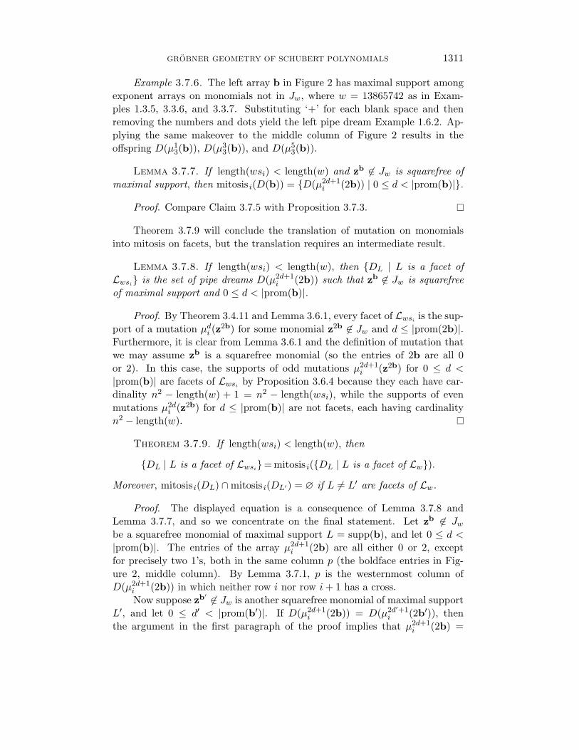
GROBNER GEOMETRY OF SCHUBERT POLYNOMIALS 1311
Example 3.7.6. The left array b in Figure 2 has maximal support amongexponent arrays on monomials not in Jw, where w = 13865742 as in Exam-ples 1.3.5, 3.3.6, and 3.3.7. Substituting ‘+’ for each blank space and thenremoving the numbers and dots yield the left pipe dream Example 1.6.2. Ap-plying the same makeover to the middle column of Figure 2 results in theoffspring D(μ1
3(b)), D(μ33(b)), and D(μ5
3(b)).
Lemma 3.7.7. If length(wsi) < length(w) and zb �∈ Jw is squarefree ofmaximal support, then mitosis i(D(b)) = {D(μ2d+1
i (2b)) | 0 ≤ d < |prom(b)|}.
Proof. Compare Claim 3.7.5 with Proposition 3.7.3.
Theorem 3.7.9 will conclude the translation of mutation on monomialsinto mitosis on facets, but the translation requires an intermediate result.
Lemma 3.7.8. If length(wsi) < length(w), then {DL | L is a facet ofLwsi
} is the set of pipe dreams D(μ2d+1i (2b)) such that zb �∈ Jw is squarefree
of maximal support and 0 ≤ d < |prom(b)|.
Proof. By Theorem 3.4.11 and Lemma 3.6.1, every facet of Lwsiis the sup-
port of a mutation μdi (z
2b) for some monomial z2b �∈ Jw and d ≤ |prom(2b)|.Furthermore, it is clear from Lemma 3.6.1 and the definition of mutation thatwe may assume zb is a squarefree monomial (so the entries of 2b are all 0or 2). In this case, the supports of odd mutations μ2d+1
i (z2b) for 0 ≤ d <
|prom(b)| are facets of Lwsiby Proposition 3.6.4 because they each have car-
dinality n2 − length(w) + 1 = n2 − length(wsi), while the supports of evenmutations μ2d
i (z2b) for d ≤ |prom(b)| are not facets, each having cardinalityn2 − length(w).
Theorem 3.7.9. If length(wsi) < length(w), then
{DL | L is a facet of Lwsi}= mitosis i({DL | L is a facet of Lw}).
Moreover, mitosis i(DL) ∩ mitosis i(DL′) = ∅ if L �= L′ are facets of Lw.
Proof. The displayed equation is a consequence of Lemma 3.7.8 andLemma 3.7.7, and so we concentrate on the final statement. Let zb �∈ Jw
be a squarefree monomial of maximal support L = supp(b), and let 0 ≤ d <
|prom(b)|. The entries of the array μ2d+1i (2b) are all either 0 or 2, except
for precisely two 1’s, both in the same column p (the boldface entries in Fig-ure 2, middle column). By Lemma 3.7.1, p is the westernmost column ofD(μ2d+1
i (2b)) in which neither row i nor row i + 1 has a cross.Now suppose zb′ �∈ Jw is another squarefree monomial of maximal support
L′, and let 0 ≤ d′ < |prom(b′)|. If D(μ2d+1i (2b)) = D(μ2d′+1
i (2b′)), thenthe argument in the first paragraph of the proof implies that μ2d+1
i (2b) =

1312 ALLEN KNUTSON AND EZRA MILLER
μ2d′+1i (2b′), since they have the same entries equal to 1 as well as the same
support, and all of their other nonzero entries equal 2. We conclude that b = b′
by Lemma 3.4.4. Using Lemma 3.7.8, we have proved that mitosis i(DL) ∩mitosis i(DL′) �= ∅ implies L = L′.
Example 3.7.10. The pipe dream D in Example 3.7.6 and the left sideof Example 1.6.2 is DL for a facet of L13865742. By Theorem 3.7.9, the threepipe dreams at the right of Example 1.6.2 can be expressed as DL′ for facetsL′ ∈ L13685742, where 13685742 = 13865742 · s3.
3.8. Facets and reduced pipe dreams
To derive the connection between the initial complex Lw and reducedpipe dreams, in Theorem 3.8.5, we need the next result, whose proof connectschuting with antidiagonals.
Lemma 3.8.1. The set {DL | L ∈ facets(Lw)} is closed under chutemoves.
Proof. A pipe dream D is equal to DL for some (not necessarily maximal)L ∈ Lw if and only if D meets every antidiagonal in Jw, which by definitionof Lw equals
⋂L∈Lw
〈zqp | (q, p) ∈ DL〉. Suppose that C is a chutable rectanglein DL for L ∈ Lw. It is enough to show that the intersection a ∩ DL of anyantidiagonal a ∈ Jw with DL does not consist entirely of the single cross inthe northeast corner of C, unless a also contains the southwest corner of C.Indeed, the purity of Lw (Proposition 3.6.4) will then imply that chuting DL
in C yields DL′ for some facet L′ whenever L ∈ facets(Lw).To prove the claim concerning a ∩ DL, we may assume a contains the
cross in the northeast corner (q, p) of C, but not the cross in the southwestcorner of C, and splits into cases:
(i) a does not continue south of row q.
(ii) a continues south of row q but skips row q + 1.
(iii) a intersects row q + 1, but strictly east of the southwest corner of C.
(iv) a intersects row q + 1, but strictly west of the southwest corner of C.
Letting (q + 1, t) be the southwest corner of C, construct new antidiagonals a′
that are in Jw (and hence intersect DL) by replacing the cross at (q, p) with across at:
(i) (q, t), using Lemma 3.3.3(W);
(ii) (q + 1, p), using Lemma 3.3.3(S);

GROBNER GEOMETRY OF SCHUBERT POLYNOMIALS 1313
(iii) (q, p), so a = a′ trivially; or
(iv) (q, t), using Lemma 3.3.3(W).
Observe that in case (iii), a already shares a box in row q + 1 where DL hasa cross. Each of the other antidiagonals a′ intersects both a and DL in somebox that is not (q, p), since the location of a′ � a has been constructed not tobe a cross in DL.
Lemma 1.4.5 implies the following criterion for when removing a ‘+’ froma pipe dream D ∈ RP(w) yields a pipe dream in RP(wsi). Specifically, itconcerns the removal of a cross at (i, j) from configurations that look like
1 · · · j
i . . .i+1 ��
=
1 · · · j
i + + + + + + + + . . .i+1 + + + + + + + ·
at the west end of rows i and i + 1 in D.
Lemma 3.8.2. Let D ∈ RP(w) and j be a fixed column index with(i + 1, j) �∈ D, but (i, p) ∈ D for all p ≤ j, and (i + 1, p) ∈ D for all p < j.Then length(wsi) < length(w), and if D′ = D � (i, j) then D′ ∈ RP(wsi).
Proof. Removing (i, j) only switches the exit points of the two pipesstarting in rows i and i + 1, so the pipe starting in row k of D′ exits out ofcolumn wsi(k) for each k. The result follows from Lemma 1.4.5.
The connection beween the complexes Lw and reduced pipe dreams re-quires certain facts proved by Bergeron and Billey [BB93]. The next lemmaconsists mostly of the combinatorial parts (a), (b), and (c) of [BB93, Th. 3.7],their main result. Its proof there relies exclusively on elementary properties ofreduced pipe dreams.
Lemma 3.8.3 ([BB93]).
1. The set RP(w) of reduced pipe dreams for w is closed under chute oper-ations.
2. There is a unique top reduced pipe dream for w such that every crossnot in the first row has a cross due north of it.
3. Every reduced pipe dream for w can be obtained by applying a sequenceof chute moves to the top reduced pipe dream for w.
Lemma 3.8.4. The top reduced pipe dream for w is DL for a facet L ∈ Lw.

1314 ALLEN KNUTSON AND EZRA MILLER
Proof. The unique reduced pipe dream for w0, whose crosses lie at {(q, p) |q + p ≤ n}, is also DL for the unique facet of Lw0 . By Lemma 3.6.3, take w
and wsi as in Lemma 3.6.2 and assume the result for w. By Lemma 3.6.3again, the top pipe dream D ∈ RP(w) satisfies the conditions of Lemma 3.8.2,where α lies at (i + 1, j). Now combine Lemma 3.8.2 with the last sentence ofLemma 3.6.2 to prove the desired result for wsi.
Theorem 3.8.5. RP(w) = {DL | L is a facet of Lw}, where DL =[n]2�L. In other words, reduced pipe dreams for w are complements of maximalsupports of monomials �∈ Jw.
Proof. Lemma 3.8.4 and Lemma 3.8.1 imply that RP(w) ⊆ {DL | L ∈facets(Lw)}, given Lemma 3.8.3. Since the opposite containment {DL | L ∈facets(Lv)} ⊆ RP(v) is obvious for v = w0, it suffices to prove it for v = wsi
by assuming it for v = w.A pair (i+1, j) as in Lemma 3.8.2 exists in D if and only if the set J (D) in
Definition 1.6.1 is nonempty, which occurs if and only if mitosis i(D) �= ∅. Inthis case, the first offspring of D under mitosis i (as in Proposition 3.7.3) is D′ =D � (i, j) ∈ RP(wsi). The desired containment follows from Theorem 3.7.9and statement 1 of Lemma 3.8.3.
3.9. Proofs of Theorems A, B, and C
In this section, we tie up loose ends, completing the proofs of Theorems A,B, and C. All statements in these theorems are straightforward for the longpermutation w = w0, so we may prove the rest by Bruhat induction—that is,by downward induction on length(w).
The multidegrees of {Xw}w∈Snof matrix Schubert varieties satisfy the
divided difference recursion defining double Schubert polynomials by Theo-rem 3.2.8. Separately, the Hilbert series of {k[z]/Jw}w∈Sn
satisfy the Demazurerecursion defining the double Grothendieck polynomials by Theorem 3.5.4. Itfollows by Lemma 1.1.4 that the multidegrees {[Lw]}w∈Sn
satisfy the divideddifference recursion.
The subspace arrangement Lw is equidimensional by Proposition 3.6.4,and the multidegree of Xw equals that of k[z]/in(I(Xw)) under any term or-der, by degeneration in Theorem 1.7.1. Moreover, if the term order is antidi-agonal, then Jw ⊆ in(Iw) ⊆ in(I(Xw)), whence Jw = in(Iw) = in(I(Xw)) byLemma 1.7.5 with I ′ = in(I(Xw)) and J = Jw. The primality of Iw in The-orem A follows because in(Iw) = in(I(Xw)) and Iw ⊆ I(Xw). The Grobnerbasis statement in Theorem B is an immediate consequence. Hilbert series arepreserved under taking initial ideals, so the K-polynomials and multidegrees of
GROBNER GEOMETRY OF SCHUBERT POLYNOMIALS 1315
{k[z]/Iw}w∈Snsatisfy the Demazure and divided difference recursions, proving
Theorem A.The last sentence of Theorem B is Theorem 3.8.5. Using that, we con-
clude the remaining statement in Theorem B, namely shellability and Cohen–Macaulayness, by applying Theorem E to Example 1.8.3. Mitosis in Theorem Ccomes from applying Theorem 3.8.5 to the mitosis in Theorem 3.7.9.
University of California, Berkeley, CA
E-mail address: [email protected]
Mathematical Sciences Research Institute, Berkeley, CA
Current address: School of Mathematics, University of Minnesota,
Minneapolis, MN
E-mail address: [email protected]
References
[Abh88] S. S. Abhyankar, Enumerative Combinatorics of Young Tableaux , Marcel DekkerInc., New York, 1988.
[AK89] S. Abhyankar and D. M. Kulkarni, On Hilbertian ideals, Linear Algebra Appl . 116(1989), 53–79.
[BB82] W. Borho and J.-L. Brylinski, Differential operators on homogeneous spaces. I.Irreducibility of the associated variety for annihilators of induced modules, Invent.Math. 69 (1982), 437–476.
[BB85] ———, Differential operators on homogeneous spaces. III. Characteristic varietiesof Harish–Chandra modules and of primitive ideals, Invent. Math. 80 (1985), 1–68.
[BB93] N. Bergeron and S. Billey, RC-graphs and Schubert polynomials, ExperimentalMath. 2 (1993), 257–269.
[BC98] W. Bruns and A. Conca, KRS and powers of determinantal ideals, CompositioMath. 111 (1998), 111–122.
[BC01] ———, KRS and determinantal ideals, in Geometric and Combinatorial Aspectsof Commutative Algebra (Messina, 1999), 67–87, Lecture Notes in Pure and Appl.Math. 217, Dekker, New York, 2001.
[Ber92] N. Bergeron, A combinatorial construction of the Schubert polynomials, J. Combin.Theory Ser. A 60 (1992), 168–182.
[BGG73] I. N. Bernsteın, I. M. Gel′fand, and S. I. Gel
′fand, Schubert cells, and the coho-
mology of the spaces G/P , Uspehi Mat. Nauk 28 (1973), 3–26.
[BH93] W. Bruns and J. Herzog, Cohen-Macaulay Rings, Cambridge Studies in AdvancedMath. 39, Cambridge Univ. Press, Cambridge, 1993.
[BJS93] S. C. Billey, W. Jockusch, and R. P. Stanley, Some combinatorial properties ofSchubert polynomials, J. Algebraic Combin. 2 (1993), 345–374.
[BKL85] A. Bjorner, B. Korte, and L. Lovasz, Homotopy properties of greedoids, Adv. inAppl. Math. 6 (1985), 447–494.
[BL00] S. Billey and V. Lakshmibai, Singular Loci of Schubert Varieties, Birkhauser BostonInc., Boston, MA, 2000.
[Bor53] A. Borel, Sur la cohomologie des espaces fibres principaux et des espaces homogenesde groupes de Lie compacts, Ann. of Math. 57 (1953), 115–207.
1316 ALLEN KNUTSON AND EZRA MILLER
[BP79] L. J. Billera and J. S. Provan, A decomposition property for simplicial complexesand its relation to diameters and shellings, Second International Conference onCombinatorial Mathematics (New York, 1978), New York Acad. Sci., New York,1979, pp. 82–85.
[BS02] N. Bergeron and F. Sottile, A Pieri-type formula for isotropic flag manifolds,Trans. Amer. Math. Soc. 354 (2002), 2659–2705 (electronic).
[BW82] A. Bjorner and M. Wachs, Bruhat order of Coxeter groups and shellability, Adv.in Math. 43 (1982), 87–100.
[CGG90] L. Caniglia, J. A. Guccione, and J. J. Guccione, Ideals of generic minors, Comm.Algebra 18 (1990), 2633–2640.
[CH94] A. Conca and J. Herzog, On the Hilbert function of determinantal rings and theircanonical module, Proc. Amer. Math. Soc. 122 (1994), 677–681.
[CH97] ———, Ladder determinantal rings have rational singularities, Adv. Math. 132(1997), 120–147.
[Con95] A. Conca, Ladder determinantal rings, J. Pure Appl. Algebra 98 (1995), 119–134.
[Dem74] M. Demazure, Desingularisation des varietes de Schubert generalisees, Ann. Sci.Ecole Norm. Sup. 7 (1974), 53–88.
[EG98] D. Edidin and W. Graham, Equivariant intersection theory, Invent. Math. 131(1998), 595–634.
[Ehr34] C. Ehresmann, Sur la topologie de certains espaces homogenes, Ann. of Math. 35(1934), 396–443.
[Eis95] D. Eisenbud, Commutative algebra, with a view toward algebraic geometry, Grad-uate Texts in Math. 150, Springer-Verlag, New York, 1995.
[ER98] J. A. Eagon and V. Reiner, Resolutions of Stanley-Reisner rings and Alexanderduality, J. Pure Appl. Algebra 130 (1998), 265–275.
[FK94] S. Fomin and A. N. Kirillov, Grothendieck polynomials and the Yang-Baxter equa-tion, Proc. Sixth Conference in Formal Power Series and Algebraic Combinatorics,DIMACS, 1994, 183–190.
[FK96] ———, The Yang-Baxter equation, symmetric functions, and Schubert polynomi-als, Discrete Math. 153 (1996), 123–143, Proc. Fifth Conf. Formal Power Seriesand Algebraic Combinatorics (Florence, 1993).
[FR02] L. Feher and R. Rimanyi, Schur and Schubert polynomials as Thom polynomials–cohomology of moduli spaces, Cent. Eur. J. Math. 1 (2003), 418–434 (electronic).
[FS94] S. Fomin and R. P. Stanley, Schubert polynomials and the nil-Coxeter algebra, Adv.Math. 103 (1994), 196–207.
[Ful92] W. Fulton, Flags, Schubert polynomials, degeneracy loci, and determinantal for-mulas, Duke Math. J . 65 (1992), 381–420.
[Ful98] ———, Intersection Theory , second ed., Springer-Verlag, New York, 1998.
[GC50] I. M. Gel′fand and M. L. Cetlin, Finite-dimensional representations of the group
of unimodular matrices, Dokl. Akad. Nauk SSSR 71 (1950), 825–828.
[Gho02] S. R. Ghorpade, Hilbert functions of ladder determinantal varieties, Discrete Math.246 (2002), 131–175, Formal power series and algebraic combinatorics (Barcelona,1999).
[GL97] N. Gonciulea and V. Lakshmibai, Schubert varieties, toric varieties, and ladderdeterminantal varieties, Ann. Inst. Fourier (Grenoble) 47 (1997), 1013–1064.
GROBNER GEOMETRY OF SCHUBERT POLYNOMIALS 1317
[GL00] N. Gonciulea and V. Lakshmibai, Singular loci of ladder determinantal varieties andSchubert varieties, J. Algebra 229 (2000), 463–497.
[GM00] N. Gonciulea and C. Miller, Mixed ladder determinantal varieties, J. Algebra 231(2000), 104–137.
[GS83] V. Guillemin and S. Sternberg, The Gel′fand-Cetlin system and quantization ofthe complex flag manifolds, J. Funct. Anal . 52 (1983), 106–128.
[HT92] J. Herzog and N. Trung, Grobner bases and multiplicity of determinantal andPfaffian ideals, Adv. Math. 96 (1992), 1–37.
[Hum90] J. E. Humphreys, Reflection Groups and Coxeter Groups, Cambridge UniversityPress, Cambridge, 1990.
[Jos84] A. Joseph, On the variety of a highest weight module, J. Algebra 88 (1984), 238–278.
[Jos97] ———, Orbital varieties, Goldie rank polynomials and unitary highest weight mod-ules, in Algebraic and Analytic Methods in Representation Theory (Sonderborg,1994), 53–98, Perspect. Math. 17, Academic Press, San Diego, CA, 1997.
[Kaz97] M. E. Kazarian, Characteristic classes of singularity theory, The Arnold-GelfandMathematical Seminars, Birkhauser Boston, Boston, MA, 1997, pp. 325–340.
[KiM00] A. N. Kirillov and T. Maeno, Quantum double Schubert polynomials, quantumSchubert polynomials and Vafa–Intriligator formula, Discrete Math. 217 (2000),191–223, Formal power series and algebraic combinatorics (Vienna, 1997).
[KnM04] A. Knutson and E. Miller, Subword complexes in Coxeter groups, Adv. in Math.184 (2004), 161–176.
[Kog00] M. Kogan, Schubert geometry of flag varieties and Gel′fand-Cetlin theory, Ph.D.thesis, Massachusetts Institute of Technology, 2000.
[KoM03] M. Kogan and E. Miller, Toric degeneration of Schubert varieties and Gel′fand–Tsetlin polytopes, Adv. in Math., in press; arXiv:math.AG/0303208
[Koh91] A. Kohnert, Weintrauben, Polynome, Tableaux, Bayreuth. Math. Schr. (1991),no. 38, 1–97, Dissertation, Universitat Bayreuth, Bayreuth, 1990.
[KP99] C. Krattenthaler and M. Prohaska, A remarkable formula for counting noninter-secting lattice paths in a ladder with respect to turns, Trans. Amer. Math. Soc.351 (1999), 1015–1042.
[KS95] M. Kalkbrener and B. Sturmfels, Initial complexes of prime ideals, Adv. Math.116 (1995), 365–376.
[Las90] A. Lascoux, Anneau de Grothendieck de la variete de drapeaux, in The GrothendieckFestschrift , Vol. III, Birkhauser Boston, Boston, MA, 1990, pp. 1–34.
[LS82a] A. Lascoux and M.-P. Schutzenberger, Polynomes de Schubert, C. R. Acad. Sci.Paris Ser. I Math. 294 (1982), 447–450.
[LS82b] ———, Structure de Hopf de l’anneau de cohomologie et de l’anneau deGrothendieck d’une variete de drapeaux, C. R. Acad. Sci. Paris Ser. I Math. 295(1982), 629–633.
[Mac91] I. G. Macdonald, Notes on Schubert Polynomials, Publications du LACIM, Univer-site du Quebec a Montreal, 1991.
[Mar02] J. Martin, Graph varieties, Ph.D. thesis, University of California at San Diego,2002.
[Mil03] E. Miller, Mitosis recursion for coefficients of Schubert polynomials, J. Combin.Theory Ser. A 101 (2003), 223–235.

1318 ALLEN KNUTSON AND EZRA MILLER
[MS96] J. V. Motwani and M. A. Sohoni, Divisor class groups of ladder determinantalvarieties, J. Algebra 186 (1996), 338–367.
[Mul89] S. B. Mulay, Determinantal loci and the flag variety, Adv. Math. 74 (1989), 1–30.
[Ram85] A. Ramanathan, Schubert varieties are arithmetically Cohen-Macaulay, Invent.Math. 80 (1985), 283–294.
[Ros89] W. Rossmann, Equivariant multiplicities on complex varieties, Orbites unipotenteset representations, III, Asterisque 11, No. 173–174 (1989), 313–330.
[RR85] S. Ramanan and A. Ramanathan, Projective normality of flag varieties and Schubertvarieties, Invent. Math. 79 (1985), 217–224.
[Stu90] B. Sturmfels, Grobner bases and Stanley decompositions of determinantal rings,Math. Z. 205 (1990), 137–144.
[Tot99] B. Totaro, The Chow ring of a classifying space, in Algebraic K-theory (Seattle,WA, 1997), Amer. Math. Soc., Providence, RI, 1999, pp. 249–281.
[Win99] R. Winkel, Diagram rules for the generation of Schubert polynomials, J. Combin.Theory Ser. A 86 (1999), 14–48.
(Received January 25, 2002)


![Gr¨obner bases - Eindhoven University of Technologyamc/pub/grobner/gbnp.pdf · Gr¨obner bases In [6] Mora described an algorithm which, if it terminates, returns a non-commutative](https://static.fdocuments.in/doc/165x107/5f1f6dff25d39e3da305c509/grobner-bases-eindhoven-university-of-amcpubgrobnergbnppdf-grobner-bases.jpg)