Grid Scheduling Divisible Loads from Two

Sources

M.A. Moges

Department of Engineering Technology, University of Houston, Houston, TX

77204, Tel. 713-743 4034, Fax. 713-743 4032

D. Yu

Department of Physics, Brookhaven National Laboratory, Upton, NY 11973

T.G. Robertazzi ∗

Department of Electrical and Computer Engineering, Stony Brook University,

Stony Brook, NY 11794, Tel. 631-632 8412, Fax. 631-632 8494

Abstract

To date closed form solutions for optimal finish time and job allocation are largely

obtained only for network topologies with a single load originating (root) proces-

sor. However in large-scale data intensive problems with geographically distributed

resources, load is generated from multiple sources. This paper introduces a new

divisible load scheduling strategy for single level tree networks with two load origi-

nating processors. Solutions for an optimal allocation of fractions of load to nodes

in single level tree networks are obtained via linear programming. A unique schedul-

ing strategy that allows one to obtain closed form solutions for the optimal finish

time and load allocation for each processor in the network is also presented. The

Preprint submitted to Elsevier Science 30 June 2009

tradeoff between linear programming and closed form solutions in terms of under-

lying assumptions is examined. Finally, a performance evaluation of a two source

homogeneous single level tree network with concurrent communication strategy is

presented.

Key words: Divisible loads, Grid scheduling, Multiple sources, Optimal

scheduling, Tree networks

1 Introduction

The problem of minimizing the processing time of extensive processing loads

originating from a multiplicity of sources and being processed on a multiplicity

of nodes presents a challenge that, if successfully met, could foster a range of

new creative applications. Inspired by this challenge, we discuss in this paper

a representative scheduling model and solutions for two sources distributing

load into a grid of a finite number of processors. Almost all work to date on

divisible load scheduling has involved models with a single nodal source of

load.

Our intent is not to propose one model to ”fit all” problems but rather to

indicate some of the modeling possibilities involving divisible load and more

than one source of load. Certainly other models with a variety of assumptions

are possible but this is beyond the scope of this paper whose purpose is to

propose a foundation for further elaboration.

∗ Corresponding author.Email addresses: mmoges@uh.edu (M.A. Moges), dtyu@bnl.gov (D. Yu),

tom@.ece.sunysb.edu (T.G. Robertazzi).

2

A growing literature on grid scheduling has appeared over the past several

years. Some representative work is now discussed. There is work on general

architectures in [1]. Prediction involving local grid scheduling [2], queue wait

times [3] and variance [4] have been studied. The decoupling of computation

and data scheduling is the subject of [5]. Grid scheduling research has involved

such features as multiple simultaneous requests [6], memory consciousness [7],

fault tolerance [8], incentives [9] and biological concepts [10]. A report on

scheduling experiences with parameter sweep applications appears in [11]. A

study showing a comparison of grid scheduling algorithms for coarse grain

independent tasks appears in [12].

The mathematical theory of divisible loads is uniquely suited to serve as a basis

for analytically modeling and solving grid scheduling problems in its ability to

capture both computing and communication in a single model. Divisible load

theory [13,14,15] is characterized by the fine granularity and large volume of

loads. There are also no precedence relations among the data elements. Such

a load may be arbitrarily partitioned and distributed among processors and

links in a system. The approach is particularly suited to the processing of

very large data files in signal processing, image processing, experimental data

processing, grid computing and computer utility applications.

There has been an increasing amount of study in divisible load theory since

the original work of Cheng and Robertazzi [16] in 1988. The majority of these

studies develop an efficient load distribution strategy and protocol in order

to achieve optimal processing time in networks with a single root processor.

The optimal solution is obtained by forcing the processors over a network

to all stop processing simultaneously. Intuitively, this is because the solution

could be improved by transferring load if some processors were idle while

3

other are still busy [17]. Such studies for network topologies including linear

daisy chains, tree and bus networks using a set of recursive equations were

presented in [16,18,19] respectively. There have been further studies in terms

of load distribution policies for hypercubes [20] and mesh networks [21]. The

concept of equivalent networks [22] was presented for complex networks such

as multilevel tree networks. Work has also considered scheduling policy with

multi-installment [23], multi-round algorithms [24], independent task schedul-

ing [25], fixed communication charges [26], detailed parameterizations and

solution reporting time optimization [27] and combinatorial optimization [28].

Recently, though divisible load theory is fundamentally a deterministic theory,

a study has been done to show some equivalence to Markov chain models [29].

There is a limited amount of literature on divisible load modeling with multiple

sources. A 2002 paper on multi-source load distribution combining Markovian

queueing theory and divisible load scheduling theory is by Ko and Robertazzi

[30]. In 2003 Wong, Yu, Veeravalli and Robertazzi [31] examined two source

grid scheduling with memory capacity constraints. Marchal, Yang, Casanova

and Robert [32] in 2005 studied the use of linear programming to maximize

throughput for large grids with multiple loads/sources. In 2005, Lammie and

Robertazzi [33] presented a numerical solution for a linear daisy chain network

with load originating at both ends of the chain. Finally, Yu and Robertazzi

examined mathematical programming solutions and flow structure in multi-

source problems in 2006 [34].

A word is in order on the type of load distribution examined in this paper.

Two types of load distribution, sequential and concurrent, have been studied

in the literature to date when there is a single nodal source of load. Sequential

distribution, where a node can only distribute to one child at a time, has

4

received the majority of study. Under concurrent load distribution, load is

distributed to all children simultaneously.

Sequential load distribution is implicit in bus networks and makes sense there

and in tree networks when the output port hardware is capable of only se-

quential distribution. In fact sequential distribution leads to interesting op-

timization problems involving finding the best load distribution order that

minimizes solution time and maximizes speedup. If it can be supported by

output port hardware, concurrent load distribution [35,36] has a higher the-

oretical throughput than sequential distribution. In fact concurrent load dis-

tribution makes practical sense for large grid applications, such as the new

ATLAS physics experiment at CERN. With voluminous amounts of experi-

mental data being distributed from the CERN site in Switzerland to other

continents, one would like all of the links to these distant sites to operate si-

multaneously to boost the utilization of facilities. One would be hard pressed

trying to explain to one’s manager why sequential distribution, with only one

link active at a time, should be implemented in this context.

The organization of this paper is as follows. In section 2, the system model

used in this paper is discussed. The analysis of the optimal finish time in

single level tree networks for concurrent communication strategy is presented

in section 3. Section 4 presents the respective performance evaluation results

in terms of finish time. Finally the conclusion appears in section 5.

5

2 Two Root Processors System Model

In this section, the various network parameters used in this paper are presented

along with some notation and definitions. The network topology discussed in

this study is a tree network consisting of two root processors (P1 and P2) and

N − 2 child processors (P3, ... , PN) with 2(N − 2) links as shown in Figure

1. It will be assumed that the total processing load considered here is of the

arbitrarily divisible kind that can be partitioned into fractions of loads to

be assigned to each processor over a network. The two root processors keep

their own fraction of loads (α1 and α2) and communicate/distribute the other

fractions of loads (α3, α4, ... αN) assigned to the rest of processors in the

network. Each processor begins to process its share of the load once the load

share from either root processor has been completely received.

The load distribution strategy from a root processor to the child processors

may be sequential or concurrent. In the sequential load distribution strategy,

each root processor is able to communicate with only one child at a time. How-

ever, in the case of concurrent communication strategy, each root processor

can communicate simultaneously/concurrently with all the child processors.

The latter communication strategy can be implemented by using a processor

which has a CPU that loads an output buffer for each output link. In this

case it can be assumed that the CPU distributes the load to all of its output

buffers at a rapid enough rate so that the buffer outputs are concurrent.

6

P1 P2

P4 PN

z13 z1N

z23

z2N

P3

z14 z24

root processor 1 root processor 2

Fig. 1. Single level tree network with two root processors.

2.1 Notations and Definitions:

Li: Total processing load originated from root processor i, (i = 1, 2).

αi: The total fraction of load that is assigned by the root processors to child

i.

α1i: The fraction of load that is assigned to processor i by the first root pro-

cessor.

α2i: The fraction of load that is assigned to processor i by the second root

processor.

αi = α1i + α2i, i = 3, 4, ..., N.

ωi: A constant that is inversely proportional to the processing speed of pro-

cessor i in the network.

zi: A constant that is inversely proportional to the speed of link i in the net-

7

work.

z1i: A constant that is inversely proportional to the speed of link between the

first root processor and the ith child processor in the network.

z2i: A constant that is inversely proportional to the speed of link between the

second root processor and the ith child processor in the network.

Tcp: Processing intensity constant. This is the time it takes the ith processor

to process the entire load when ωi = 1. The entire load can be processed

on the ith processor in time ωiTcp.

Tcm: Communication intensity constant. This is the time it takes to transmit

all the processing load over a link when zi = 1. The entire load can be

transmitted over the ith link in time ziTcm.

Ti: The total time that elapses between the beginning of the scheduling pro-

cess at t = 0 and the time when processor i completes its processing,

i = 1, ..., N . This includes communication time, processing time and idle

time.

Tf : This is the time when the last processor finishes processing.

Tf = max(T1,T2, . . . , TN).

8

One convention that is followed in this paper is that the total load originating

at the two root processors is assumed to be normalized to be a unit load. That

is,

L1 + L2 = 1.

3 Optimal Scheduling Strategies

The load scheduling strategies presented here target finding solutions for op-

timal finish time (make-span) and job allocation in single level tree networks

with two root processors. Most previous load scheduling strategies in divisible

load models can be solved algebraically in order to find the optimal finish time

and load allocation to processors and links. In this case optimality is defined

in the context of the specific interconnection topology and load distribution

schedule used. An optimal solution is usually obtained by forcing all proces-

sors to finish computing at the same time. This yields an optimal solution as,

intuitively by contradiction, if there exist idle processors in the network, load

can be transferred from busy processors to those idle processors [17]. This

section covers some representative load scheduling strategies for single level

tree networks with two root processors. A brief mention of a single level tree

network with one root processor is also presented in order to find and compare

the performance improvement.

9

P1

P2

a1w1Tcp

a2w2Tcp

computation

communication Tf

Tf

concurrent

P3 a3w3Tcp

Tf

PN aNwNTcp

Tf

aN zNTcm

a2z2Tcm

a3z3Tcm

Fig. 2. Timing diagram for a single level tree network with a single root processor

and concurrent communication.

3.1 Single Level Tree Network with Single Root Processor and Concurrent

Communication

A single level tree network with a single root processor consists of N processors

and N − 1 links. All the processors are connected to the root processor via

communication links. The root processor, assumed to be the only processor

at which the load arrives, partitions a total processing load into N fractions,

keeps its own fraction α1, and distributes the other fractions α2, α3, . . .

, αN to the N − 1 child processors respectively. The root processor in the

network is equipped with a front end. That is, the root can compute its own

fraction of load and communicates the rest of the load to each of its children

simultaneously. Each processor begins computing immediately after receiving

its assigned fraction of load and continues without any interruption until all

of its assigned load fraction has been processed. In this case each processor

10

begins to compute its fraction of load at the moment that it finishes receiving

its data.

The process of load distribution in a single level tree network with a single

root processor is shown in Figure 2 using Gantt-chart-like timing diagram.

The communication time is shown above the time axis and the computation

time is shown below the time axis.

The set of equations for finding the minimum finish time can be written as:

α1ω1Tcp = α2z2Tcm + α2ω2Tcp (1)

α2z2Tcm + α2ω2Tcp = α3z3Tcm + α3ω3Tcp (2)

αiziTcm + αiωiTcp = αi+1zi+1Tcm (3)

+ αi+1ωi+1Tcp

αN−1zN−1Tcm + αN−1ωN−1Tcp = αNzNTcm (4)

+ αNωNTcp

The fractions of the total processing load should sum to one.

α0 + α1 + α2 + ... + αN−1 + αN = 1 (5)

The above set of recursive equations can be used to solve the optimum fraction

of loads (α′is) that should be assigned to each of the processor. In this case

there is an equal number of equations to the number of unknowns, hence the

solution is always unique. The majority of research in this area has assumed a

single root processor like that presented in this section. The following section

11

describes a load distribution strategy for this network topology with two root

processors which is the main focus of this paper.

3.2 Single Level Tree Network with Two Root Processors and Concurrent

Communication

Two generic techniques for solving linear divisible load schedule problems are

linear programming and linear equation solution. Linear programming has the

advantage of being able to handle a wide variety of constraints and producing

numerical solutions for all types of linear models. Alternately one can often,

though not always, set up a set of linear equations that can be solved either

numerically or, in special cases, analytically. Analytical closed form solutions

have the advantage of giving insight into system dependencies and tradeoffs.

Furthermore, analytical solutions, when they can be realized, usually require

only a trivial amount of calculation.

In this section a representative two source problem with linear programming

solution is discussed. In section 3.3 further assumptions are made to achieve

a typical closed form solution.

The network topology considered here is a tree network with two root pro-

cessors and N − 2 child processors. In this case, it is assumed that the total

processing load originates from the two root processors (P1 and P2). The

scheduling strategy involves the partitioning and distribution of the process-

ing loads originated from P1 and P2 to all the processors. The load distribution

process proceeds as follows: the total processing loads originated from P1 and

P2 are assumed to be L1 and L2 respectively. Each root processor keeps some

12

P1 T1

P2

P3 T3

T2

a13z13Tcm

a14z14Tcm

P4T4

a14w4Tcp a24w4Tcp

a13w3Tcp a23w3Tcp

a23z23Tcm

a24z24Tcm

a2w2Tcp

a1w1Tcp

a1Nz1NTcm

a2Nz2NTcm

PNTN

a1NwNTcp a2NwNTcp

Fig. 3. Timing diagram for a single level tree network with two root processors and

concurrent communication.

fraction of the respective processing load for itself to compute and distributes

the remaining load simultaneously to the child processors. The timing diagram

shown in Figure 3, shows the load distribution process discussed above. The

figure shows that at time t = 0, the processors are all idle. The child proces-

sors start computation only after completely receiving their assigned fraction

of load from either of the two root processors.

Now the equations that govern the relations among various variables and pa-

rameters in the network can be written as follows:

13

T1 = α1ω1Tcp (6)

T2 = α2ω2Tcp (7)

T3 = (α13 + α23)ω3Tcp + min(α13z13Tcm, α23z23Tcm) (8)

TN = (α1N + α2N)ωNTcp + min(α1Nz1NTcm, α2Nz2NTcm). (9)

As it was mentioned earlier, since total processing load originating at the two

root processors is assumed to be normalized to a unit load, the fractions of

the total processing load should sum to one as:

L1 + L2 = 1 (10)

α1 + α2 + α3 + ... + αN−1 + αN = 1 (11)

Since

L1 = α1 +N∑

j=3

α1,j (12)

L2 = α2 +N∑

j=3

α2,j (13)

The normalization equation given above can also be written in terms of the

fraction of loads as:

α1 + α2 +N∑

j=3

α1,j +N∑

j=3

α2,j = 1 (14)

As it can be seen from the timing diagram shown in Figure 3, all processors

stop processing at the same time, thus we have:

T1 = T2 = T3 = . . . = TN

14

Based on the above set of equations, one can write the following set of N − 1

equations:

α1ω1Tcp = α2ω2Tcp (15)

α2ω2Tcp = α3ω3Tcp + α13z13Tcm (16)

α3ω3Tcp + α13z13Tcm = α4ω4Tcp (17)

+ α14z14Tcm

αN−1ωN−1Tcp + α1N−1z1N−1Tcm = αNωNTcp (18)

+ α1Nz1NTcm

As it can be seen from the above set of equations, there is a smaller number

of equations than the number of unknowns. Another N − 2 equations can be

written by setting up relationship between the fractions of loads within each

child processor as:

α23z23Tcm≤α13(z13Tcm + ω3Tcp) (19)

α24z24Tcm≤α14(z14Tcm + ω4Tcp) (20)

α2Nz2NTcm≤α1N(z1NTcm + ωNTcp) (21)

In this case, there will be 2N − 1 equations (including the normalization

equations) and 2N − 2 unknowns. This will lead us to a linear programming

problem with the objective function that minimizes the total processing time

of the network. In this case the objective function will be:

Minimize:

15

Tf = α1ω1Tcp (22)

Subject to:

α1ω1Tcp - α2ω2Tcp = 0

α2ω2Tcp - α3ω3Tcp - α13z13Tcm = 0

α3ω3Tcp + α13z13Tcm - α4ω4Tcp - α14z14Tcm = 0

.

.

αN−1ωN−1Tcp + α1N−1z1N−1Tcm - αNωNTcp - α1Nz1NTcm = 0

L1 - α1 -∑N

j=3 α1,j = 0

L2 - α2 -∑N

j=3 α2,j = 0

α23z23Tcm - α13(z13Tcm + ω3Tcp) ≤ 0

α24z24Tcm - α14(z14Tcm + ω4Tcp) ≤ 0

α2Nz2NTcm - α1N(z1NTcm + ωNTcp) ≤ 0

αi ≥ 0

The first set of equations enforce the constraints that all processors should

stop processing at the same time for the optimality condition. The inequality

set of constraints state that the child processors do their computation without

any interruption. The last equation is that the fractions of the assigned load

should be positive. Finally, the objective function is to minimize the total

processing time needed to process the loads originating from the two root

processors.

16

3.3 Illustrative Example - Scenario for a Closed Form Solution

In this section we present an example of a scheduling strategy that may result

in a closed form solution. We drive the expression for the minimum process-

ing time from the communication and processing speed parameters. We also

show that in the resulting expression it is possible to analytically eliminate the

processing speed yielding a simplified expression for the minimum processing

time. In order to obtain a closed form solution the following assumptions can

be made regarding the load distribution strategy:

- The two root processors start to communicate with all of the child processors

at the same time.

- For the same child processor, P1 terminates communication before P2.

- Each child processor starts processing after completely receiving its fraction

of load received from either root processors.

- All processors are equipped with front-end processors, so that they will be

able to communicate and process their respective load shares at the same time.

- The total communication and processing time of the fraction of load dis-

tributed by the first root processor (P1) to each of the child processors is

equal to the communication time needed to distribute the respective fractions

of load by P2 to each child processor. This can be achieved by controlling the

17

transmission duration of P2. Thus,

α2iz2iTcm = α1i(z1iTcm + ωiTcp).

where i > 2.

Though these assumptions are sufficient to produce closed form solution, one

can argue over their realism. For instance, one would have a more general

problem if children could receive load in any order, not a prefixed one. How-

ever, this problem is beyond the scope of this paper. Our purpose here is to

demonstrate the type of assumptions in a typical problem that have to be

made to achieve a closed form solution, realizing that in some cases some of

these assumptions may be overly restrictive. However, a linear programming

model and solution generally involves fewer assumptions (i.e. constraints) and

thus may be preferable to a closed form solution with more, possibly limiting

assumptions.

The process of load distribution for this situation is shown in Figure 4.

Using the above set of equations and since for i > 2,

αi = α1i + α2i, one can solve for α1i and α2i in terms of αi as:

α1i = kiαi (23)

α2i = (1− ki)αi (24)

where ki = z2iTcm/ri, and ri = z1iTcm + z2iTcm + ωiTcp.

All the above set of equations can be used to find the αi’s (i = 2, 3, ..., N) in

18

terms of α1 as:

α2 = (ω1Tcp/ω2Tcp)α1 (25)

α3 = s3α1 (26)

αi = siα1 (27)

where si = (ω1Tcpri)/(ωiTcpri + z1iTcmz2iTcm).

Now using the normalization equation, one can solve for α1 as:

α1 = 1/(1 + (ω1Tcp/ω2Tcp) +N∑

i=3

si) (28)

The scheduler (P1) will use the value of α1 to obtain the amount of data that

has to be processed by the rest of the N − 1 processors in the network.

The minimum processing time of the network will then be given as:

Tf = ω1Tcp/(1 + (ω1Tcp/ω2Tcp) +N∑

i=3

si) (29)

For a homogeneous network with ω = 1 and Tcp = Tcm =1, the minimum

processing time Tf approaches to 1/(Ns) as the number of processors N is

made to be increasingly large. To see this result analytically, one can start

from the expression:

α1 = 1/(1 + (ω1/ω2) +∑N

i=3 si).

Now as N is made to be large, α1 approaches 1/(2 + Ns) and since N >> 2

and N >> 1/s, the expression for the minimum finish time will then corre-

spondingly be reduced to 1/(Ns).

19

P1 T1

P2

P3 T3

T2

a13z13Tcm

a14z14Tcm

P4T4

a14w4Tcp a24w4Tcp

a13w3Tcp a23w3Tcp

a23z23Tcm

a24z24Tcm

a2w2Tcp

a1w1Tcp

a1Nz1NTcm

a2Nz2NTcm

PNTN

a1NwNTcp a2NwNTcp

Fig. 4. Timing diagram for a single level tree network with two root processors and

concurrent communication : Scheduling for closed form solution.

4 Processing Finish Time (Make Span) Results

This section presents the plots of finish time vs. number of processors in a

single level tree network with two root processors. The results are obtained

by using linear programming with the objective function of minimizing the

total processing time. In this case a homogeneous network is considered to

study the effect of communication and computation speed variations and the

number of processors on the total processing time.

In Figure 5, the finish time is plotted against the number of processors in the

network for different inverse bus speeds, z1 which is the communication link

between the first root processor and the child processors. The communication

link between the second root processor and the child processors is set to be

20

5 10 15 20 25 30 350.05

0.1

0.15

0.2

0.25

0.3

0.35

0.4

0.45

Number of Processors

Fin

ish

Tim

e

z1=2.5z1=2.0z1=1.5z1=1.0z1=0.5

Fig. 5. Finish time versus number of processors, for two root sources single level

homogeneous tree network and variable inverse bus speed, z1, (first root processor

links).

fixed to z2 = 1.

As mentioned earlier the total processing loads originated from P1 and P2

are assumed to be L1 and L2 respectively and equations 10 through 14 show

the details of L1 and L2. The tree network that is used to obtain the plot

in Figure 5 has a homogeneous link and processor speed. In this case ω =

2 and the values of Tcm and Tcp are also set to be equal to one. The plot

shows that a better finish time is obtained as the number of processors in the

network is increased and when the link speed is faster. This is expected as

more processors would have been involved in computation as the link speed is

increased.

The plot shown in Figure 6 shows the performance of the network when the

communication link between the first root processor and the child processors

z1 is fixed and the communication link between the second root processor and

the child processors z2 varies from 0.5 to 2.5. For these parameters, as shown

21

5 10 15 20 25 30 350.05

0.1

0.15

0.2

0.25

0.3

0.35

0.4

Number of Processors

Fin

ish

Tim

e

z2=0.5z2=1.0z2=1.5z2=2.0z2=2.5

Fig. 6. Finish time versus number of processors, for two root sources single level

homogeneous tree network and variable inverse bus speed, z2, (second root processor

links).

in the plot the finish time is the same regardless of the variation of z2. The

computation of the fraction of load that originates from the second processor

starts only after the completion of the processing load that originated from

the first processor. Thus the variation of the link speed z2 has no effect on the

total processing time. As mentioned in the earlier sections, this whole process

assumes that the nodes are always busy computing the loads originated from

the two root processors. That is, there is no idle time between computation

time.

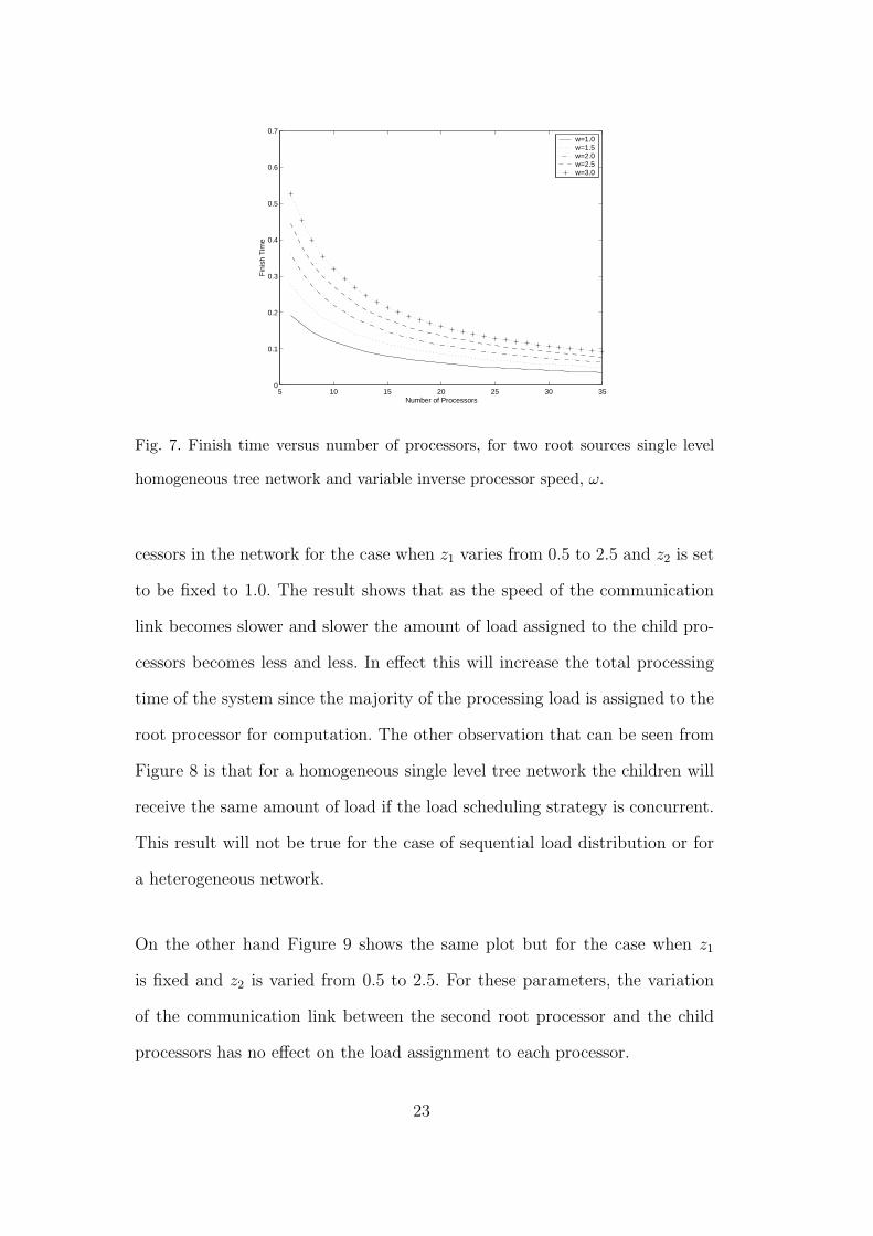
In Figure 7, the finish time is plotted against the number of processors in the

network for different inverse processor speed, ω. In this case z1 and z2 are set

to be equal to 0.5 and the values of Tcm and Tcp are set to be equal to one. The

plot shows that a better finish time is obtained as the number of processors

in the network is increased and when the processor speed is faster.

The plot shown in Figure 8 presents the load assignment to each of the pro-

22

5 10 15 20 25 30 350

0.1

0.2

0.3

0.4

0.5

0.6

0.7

Number of Processors

Fin

ish

Tim

e

w=1.0w=1.5w=2.0w=2.5w=3.0

Fig. 7. Finish time versus number of processors, for two root sources single level

homogeneous tree network and variable inverse processor speed, ω.

cessors in the network for the case when z1 varies from 0.5 to 2.5 and z2 is set

to be fixed to 1.0. The result shows that as the speed of the communication

link becomes slower and slower the amount of load assigned to the child pro-

cessors becomes less and less. In effect this will increase the total processing

time of the system since the majority of the processing load is assigned to the

root processor for computation. The other observation that can be seen from

Figure 8 is that for a homogeneous single level tree network the children will

receive the same amount of load if the load scheduling strategy is concurrent.

This result will not be true for the case of sequential load distribution or for

a heterogeneous network.

On the other hand Figure 9 shows the same plot but for the case when z1

is fixed and z2 is varied from 0.5 to 2.5. For these parameters, the variation

of the communication link between the second root processor and the child

processors has no effect on the load assignment to each processor.

23

0 5 10 15 20 25 30 350.026

0.028

0.03

0.032

0.034

0.036

0.038

0.04

0.042

0.044

0.046

Processor

Load

Ass

ignm

ent

z1=0.5z1=1.0 z1=1.5z1=2.0z1=2.5

Fig. 8. Load assignment when z1 is varied and z2 is fixed.

0 5 10 15 20 25 30 350.028

0.029

0.03

0.031

0.032

0.033

0.034

0.035

0.036

0.037

Processor

Load

Ass

ignm

ent

z2=0.5z2=1.0z2=1.5z2=2.0z2=2.5

Fig. 9. Load assignment when z1 is fixed and z2 is varied.

5 Conclusion and Open Problems

In this work we reach the following conclusions and set the stage for some

open problems.

· It has been demonstrated that one can solve the two source divisible load

scheduling problem in closed form though some of the assumptions may be

24

overly restrictive. Thus in some cases a linear programming solution with fewer

assumptions may be preferable.

· The results show that up to a certain point increasing the number of proces-

sors can significantly improve performance (i.e. makespan or finish time).

· It would be of interest to extend the two source model with concurrent

distribution in a single level tree network described here to sequential load

distribution as well as to multi-level tree networks.

· A refinement would be to rigorously define the minimal set of assumptions

that lead to a closed form solution in the two source model.

· A natural extension would be the development of a systematic set of mod-

eling equations for the N source/M sink problem under various scheduling

strategies.

The outline of what is analytically possible, and what is not, in multi-source

load distribution is starting to become clear through work such as this. This

will allow the successful targeting of future research efforts into productive

areas.

References

[1] J. Schopf, A general architecture for scheduling on the grid. Argonne National

Laboratory preprint ANL/MCS Argonne, IL 1000 - 1002 (2002).

[2] D. Spooner and et al. Local grid scheduling techniques using performance

prediction. IEEE Proceedings - Computers and Digital Techniques, 150 87-96

(2003).

25

[3] W. Smith, V. Taylor and I. Foster, Using run-time predictions to estimate

queue wait times and improve scheduler performance. Proceedings of the

Job Scheduling Strategies for Parallel Processing Conference, Lecture Notes in

Computer Science, San Juan, Puerto Rico, 1659 202-219 (1999)

[4] L. Yang, J. Schopf and I. Foster, Conservative Scheduling: Using predicted

variance to improve scheduling decisions in dynamic environments. Proceedings

of Supercomputing 03, Pheonix, Arizona , 558-664 (2003).

[5] K. Ranganathan and I. Foster, Decoupling computation and data

scheduling in distributed data-intensive applications. Proceedings of the 11th

IEEE International Symposium on High Performance Distributed Computing

(HPDC02), Edinburgh, Scotland, 352 (2002).

[6] V. Subramani, R. Kettimuthu, S. Srinivasan and P. Sadayappan, Distributed

job scheduling on computational grids using multiple simultaneous requests.

Proceedings of the 11th IEEE International Symposium on High Performance

Distributed Computing (HPDC02), Edinburgh, Scotland, 359-366 (2002).

[7] M. Wu and X. Sun, Memory conscious task partition and scheduling in grid

environments. Proceedings of the Fifth IEEE/ACM International Workshop on

Grid Computing, Pittsburgh, USA, 138-145 (2004).

[8] J. Abawajy, Fault-tolerant scheduling policy for grid computing systems.

Proceedings of the 18th International Parallel and Distributed Processing

Symposium, Santa Fe, New Mexico, 238-245 (2004).

[9] L. Xiao, Y. Zhu, L. Ni and Z. Xu, GridIS: an incentive-based grid scheduling.

Proceedings of the 19th International Parallel and Distributed Processing

Symposium, 65b (2005).

[10] A. Chakravarti, G. Baumgartner and M. Lauria, Application-specific scheduling

for the organic grid. Proceedings of the Fifth IEEE/ACM International

26

Workshop on Grid Computing, 146-155 (2004).

[11] E. Huedo, R. Montero and I. Llorente, Experiences on adaptive grid scheduling

of parameter sweep applications. Proceedings of the 12th Euromicro Conference

on Parallel, Distributed and Network-based Processing, A Coruna, Spain, 28-33

(2004).

[12] N. Fujimoto and K. Hagihara, A comparison among grid scheduling algorithms

for indepenendt coarse-grained tasks. Proceedings of the 2004 International

Symposium on Applications and the Internet, Tokyo, Japan, 674-680 (2004).

[13] V. Bharadwaj, D. Ghose, V. Mani, and T.G. Robertazzi: Scheduling Divisible

Loads in Parallel and Distributed Systems. IEEE Computer Society Press, Los

Alamitos, CA, (1996).

[14] V. Bharadwaj, D. Ghose, T.G. Robertazzi, Divisible Load Theory: A new

paradigm for load scheduling in distributed systems. Cluster Computing, 6

7-18 (2003).

[15] T.G. Robertazzi, Ten reasons to use divisible load theory. Computer, 36 63-68

(2003).

[16] Y.C. Cheng and T.G. Robertazzi, Distributed computation with

communication delays. IEEE Transactions on Aerospace and Electronic

Systems, 22 60-79 (1988).

[17] J. Sohn and T.G. Robertazzi, Optimal divisible load sharing for bus networks.

IEEE Transactions on Aerospace and Electronic Systems, 32 34-40 (1996).

[18] Y.C. Cheng and T.G. Robertazzi, Distributed computation for a tree network

with communication delays. IEEE Transactions on Aerospace and Electronic

Systems, 26 511-516 (1990).

[19] S. Bataineh and T.G. Robertazzi, Bus oriented load sharing for a network of

27

sensor driven processors. IEEE Transactions on Systems, Man and Cybernetics,

21 1202-1205 (1991).

[20] J. Blazewicz and M. Drozdowski, Scheduling divisible jobs on hypercubes.

Parallel computing, 21 1945-1956 (1996).

[21] J. Blazewicz and M. Drozdowski, The performance limits of a two dimensional

network of load sharing processors. Foundations of Computing and Decision

Sciences, 21 3-15 (1996).

[22] T.G. Robertazzi, Processor equivalence for a linear daisy chain of load sharing

processors. IEEE Transactions on Aerospace and Electronic Systems, 29 1216-

1221 (1993).

[23] V. Bharadwaj, D. Ghose, V. Mani, Multi-installment load distribution in tree

networks with delays. IEEE Transactions on Aerospace and Electronic Systems,

31 555-567 (1995).

[24] Y. Yang, H. Casanova, UMR: A Multi-Round Algorithm for Scheduling

Divisible Workloads. Proceedings of the International Parallel and Distributed

Processing Symposium (IPDPS’03), Nice, France, (2003).

[25] O. Beaumont, A. Legrand, and Y. Robert, Optimal algorithms for scheduling

divisible workloads on heterogeneous systems. 12th Heterogeneous Computing

Workshops HCW’2003, (2003).

[26] J. Blazewicz and M. Drozdowski, Distributed Processing of Distributed Jobs

with Communication Startup Costs. Discrete Applied Mathematics, 76 21-41

(1997).

[27] A.L. Rosenberg, Sharing partitionable workloads in heterogeneous NOWs:

greedier is not better. In D.S. Katz, T. Sterling, M. Baker, L. Bergman, M.

Paprzycki, and R. Buyya, editors. Cluster Computing 2001 pp. 124-131, (2001).

28

[28] P.F. Dutot, Divisible load on Heterogeneous Linear Array. Proceeding of the

International Parallel and Distributed Processing Symposium (IPDPS’03), Nice,

France, (2003).

[29] M. Moges and T. Robertazzi, Optimal divisible load scheduling and Markov

chain models. Proceedings of the 2003 Conference on Information Sciences and

Systems, Baltimore, MD, (2003).

[30] K. Ko, and T. Robertazzi, Scheduling in an Environment of Multiple Job

Submissions. Proceedings of the 2002 Conference on Information Sciences and

Systems, Princeton, NJ, (2002).

[31] H. Wong, B. Veeravalli, D. Yu and T. Robertazzi, Data Intensive Grid

Scheduling: Multiple Sources with Capacity Constraint. IASTED International

Conference on Parallel and Distributed Computing and Systems (PDCS 2003),

Marina del Rey, CA, (2003).

[32] L. Marchal, Y. Yang, H. Casanova and Y. Robert, A realistic

network/application model for scheduling loads on large-scale platforms.

Proceedings of the International Parallel and Distributed Processing Symposium,

Denver, Colorado, 48b (2005).

[33] T. Lammie and T. Robertazzi, A linear daisy chain with two divisible load

sources. Proceedings of 2005 Conference on Information Sciences and Systems,

Baltimore, MD,(2005).

[34] D. Yu and T. Robertazzi, Multi-source grid scheduling for divisible

loads. Proceedings of 2006 Conference on Information Sciences and Systems,

Princeton, NJ, (2006).

[35] D. Piriyakumar and C. Murthy, Distributed computation for a hypercube

network of sensor-driven processors with communication delaysincluding setup

time. IEEE Transactions on Systems, Man and Cybernetics, 28 245-251 (1998).

29

[36] J. Hung and T. Robertazzi, Scalable scheduling for clusters and grids using cut

through switching. International Journal of Computers and Applications, 26

147-156 (2004).

30