Grid-less Variational Bayesian Inference of Line Spectral ...

Grid-less Variational Bayesian Inference of

Line Spectral from Quantized Samples

Jiang Zhu, Qi Zhang and Xiangming Meng

Abstract

Efficient estimation of line spectral from quantized samples is of significant importance in information

theory and signal processing, e.g., channel estimation in energy efficient massive MIMO systems and

direction of arrival estimation. The goal of this paper is to recover the line spectral as well as its

corresponding parameters including the model order, frequencies and amplitudes from heavily quantized

samples. To this end, we propose an efficient grid-less Bayesian algorithm named VALSE-EP, which is a

combination of the variational line spectral estimation (VALSE) and expectation propagation (EP). The

basic idea of VALSE-EP is to iteratively approximate the challenging quantized model of line spectral

estimation as a sequence of simple pseudo unquantized models so that the VALSE can be applied. Note

that the noise in the pseudo linear model is heteroscedastic, i.e., different components having different

variances, and a variant of the VALSE is re-derived to obtain the final VALSE-EP. Moreover, to obtain

a benchmark performance of the proposed algorithm, the Cramer Rao bound (CRB) is derived. Finally,

numerical experiments on both synthetic and real data are performed, demonstrating the near CRB

performance of the proposed VALSE-EP for line spectral estimation from quantized samples.

Keywords: Variational Bayesian inference, expectation propagation, quantization, line spectral estimation,

MMSE, gridless

I. INTRODUCTION

Line spectral estimation (LSE) is a fundamental problem in information theory and statistical signal

processing which has widespread applications, e.g., channel estimation [2], direction of arrival (DOA)

estimation [3]. To address this problem, on one hand, many classical methods have been proposed, such

as the fast Fourier transform (FFT) based periodogram [4], subspace based MUSIC [5] and ESPRIT

[6]. On the other hand, to exploit the frequency sparsity of the line spectral signal, sparse representation

Jiang Zhu and Qi Zhang are with the Key Laboratory of Ocean Observation-imaging Testbed of Zhejiang Province, Ocean

College, Zhejiang University, No.1 Zheda Road, Zhoushan, 316021, China. Xiangming Meng is with Huawei Technologies, Co.

Ltd., Shanghai, 201206, China.

September 4, 2019 DRAFT

arX

iv:1

811.

0568

0v3

[cs

.IT

] 3

Sep

201

9

1

and compressed sensing (CS) based methods have been proposed to estimate frequencies for multiple

sinusoids.

Depending on the model adopted, CS based methods for LSE can be classified into three categories,

namely, on-grid, off-grid and grid-less, which also correspond to the chronological order in which they

have been developed [7]. At first, on-grid methods where the continuous frequency is discretized into a

finite set of grid points are proposed [8]. It is shown that grid based methods will incur basis mismatch

when the true frequencies do not lie exactly on the grid [9]. Then, off-grid compressed sensing methods

have been proposed. In [10], a Newtonalized orthogonal matching pursuit (NOMP) method is proposed,

where a Newton step and feedback are utilized to refine the frequency estimates. Compared to the

incremental step in updating the frequencies in NOMP, the iterative reweighted approach (IRA) [11]

estimates the frequencies in parallel, which improves the estimation accuracy at the cost of increasing

complexity. In [12], superfast LSE method is proposed based on fast Toeplitz matrix inversion algorithm.

In [13, 14], a sparse Bayesian learning method is proposed, where the grid bias and the grid are jointly

estimated [13], or the Newton method is applied to refine the frequency estimates [14]. To completely

overcome the grid mismatch problem, grid-less based methods have been proposed [15–18]. The atomic

norm-based methods involve solving a semidefinite programming (SDP) problem [19], whose computation

complexity is prohibitively high for large problem size. In [20], a grid-less variational line spectral

estimation (VALSE) algorithm is proposed, where posterior probability density function (PDF) of the

frequency is provided. In [21], the multisnapshot VALSE (MVALSE) is developed for the MMVs setting,

which also shows the relationship between the VALSE and the MVALSE.

In practice, the measurements might be obtained in a nonlinear way, either preferably or inevitably. For

example, in the mmWave multiple input multiple output (MIMO) system, since the mmWave accompanies

large bandwidths, the cost and power consumption are huge due to high precision (e.g., 10-12 bits) analog-

to-digital converters (ADCs) [22]. Consequently, low precision ADCs (often 1 − 3 bits) are adopted to

alleviate the ADC bottleneck. Another motivation is wideband spectrum sensing in bandwidth-constrained

wireless networks [23, 24]. In order to reduce the communication overhead, the sensors quantize their

measurements into a single bit, and the spectrum is estimated from the heavily quantized measurements

at the fusion center (FC). There are also various scenarios where measurements are inevitably obtained

nonlinearly such as phase retrieval [25, 26]. As a result, it is of great significance in designing efficient

nonlinear LSE algorithms. This paper will consider in particular LSE from low precision quantized

observations [27, 28] but extension to general nonlinear scenarios could easily fit into our proposed

framework without much difficulty.


2

A. Related Work

Many classical methods have been extended to solve the LSE from quantized samples. In [29], the

spectrum of the one-bit data is analyzed, which consists of plentiful harmonics. It shows that under low

signal to noise ratio (SNR) scenario, the amplitudes of the higher order harmonics are much smaller

than that of the fundamental frequency, thus the classical FFT based method still works well for the

SAR imaging experiment. However, the FFT based method can overestimate the model order (number

of spectrums) in the high SNR scenario. As a consequence, the quantization effects must be taken into

consideration. The CS based methods have been proposed to solve the LSE from quantized samples,

which can also be classified into on-grid, off-grid and grid-less methods.

• on-grid methods: The on-grid methods can be classified into l1 minimization based approach [30–32]

and generalized sparse Bayesian learning (Gr-SBL) [33] algorithm. For l1 minimization approach, the

regularization parameter is hard to determine the tradeoff between the fitting error and the sparsity.

While the reconstruction accuracy of the Gr-SBL is high, its computation complexity is high since

it involves a matrix inversion in each iteration.

• off-grid methods: The SVM based [34] and 1bRelax algorithm [35] are two typical approaches. For

the SVM based approach, the model order needs to be known a priori, while the 1bRelax algorithm

[36] get rid of such need by using the consistent Bayesian information criterion (BIC) to determine

the model order.

• grid-less methods: The grid-less approach can completely overcome the grid mismatch problem and

the atomic norm minimization approach has been proposed [37–39]. However, its computational

complexity is high as it involves solving a SDP.

From the point of view of CS, many Bayesian algorithms have been developed, such as approximate

message passing (AMP) [43, 44], vector AMP (VAMP) [48]. It is shown in [45, 46] that AMP can be

alternatively derived via expectation propagation (EP) [40] , an effective approximate Bayesian inference

method. To deal with nonlinear observations, i.e., generalized linear models (GLM), AMP and VAMP

are extended to GAMP [47] and GVAMP [49] respectively using different methods. The authors in [41]

propose a unified Bayesian inference framework for the GLM inference which shows that GLM could be

iteratively approximated as a standard linear model (SLM) using EP 1. This unified framework provides

new insights into some existing algorithms, as elucidated by a concise derivation of GAMP in [41], and

motivates the design of new algorithms such as the generalized SBL (Gr-SBL) algorithm [33, 41]. This

paper extends the idea further and utilize EP to solve LSE from quantized samples.

1The extrinsic message in [41] could be equivalently obtained through EP.


3

B. Main Contributions

This work studies the LSE problem from quantized measurements. Utilizing the EP [40], the gen-

eralized linear model can be iteratively decomposed as two modules (a standard linear model 2 and a

componentwise minimum mean squared error (MMSE) module) [41]. Thus the VALSE algorithm is run

in the standard linear module where the frequency estimate is iteratively refined. For the MMSE module,

it refines the pseudo observations of the linear model 3. By iterating between the two modules, the

estimates of the frequency are improved gradually. The main contributions of this work are summarized

as follows:

• A VALSE-EP method is proposed to deal with the LSE from quantized samples. The quantized

model is iteratively approximated as a sequence of pseudo unquantized models with heteroscedastic

noise (different components having different variance), a variant of the VALSE is re-derived.

• The VALSE-EP is a completely grid-less approach. Besides, the model order estimation is cou-

pled within the iteration and the computational complexity is low, compared to the atomic norm

minimization approach.

• The relationship between VALSE and VALSE-EP is revealed under the unquantized case. It is shown

that the major difference lies in the noise variance estimation step. For VALSE-EP, it is iteratively

solved by exchanging extrinsic information between the pseudo unquantized module (module A)

and the MMSE module (module B). For VALSE, the noise variance estimate is equivalently derived

through the expectation maximization (EM) step in module A, while VALSE-EP utilizes the EM

step to estimate the noise variance in module B, which demonstrate that VALSE and VALSE-EP

are not exactly equivalent.

• Utilizing the framework from [41], VALSE-EP is proposed which combines the VALSE algorithm

with EP. The two different criterions are combined together, and numerical experiments on both

synthetic and real data demonstrate the excellent performance of VALSE-EP.

• Although this paper focuses on the case of quantized measurements, it is believed that VALSE-EP

can be easily extended to other nonlinear measurement scenarios such as phase retrieval without

overcoming much difficulty.

2In fact, it is a nonlinear model instead of a standard linear model, which is different from [41] since the frequencies are

unknown.3Iteratively approximating the generalized linear model as a standard linear model is very beneficial, as many well developed

methods such as the information-theoretically optimal successive interference cancellation (SIC) is developed in the SLM.


4

C. Paper Organization and Notation

The rest of this paper is organized as below. Section II describes the system model and introduces

the probabilistic formulation. Section III derives the Cramer Rao bound (CRB). Section IV develops the

VALSE for heterogenous noise. The VALSE-EP algorithm and the details of the updating expressions

are presented in Section V. The relationship between VALSE and VALSE-EP in the unquantized setting

is revealed in Section VI. Substantial numerical experiments are provided in Section VII and Section

VIII concludes the paper.

For a complex vector x ∈ CM , let <x and =x denote the real and imaginary part of x, respectively,

let |x| and ∠x denote the componentwise amplitude and phase of x, respectively. For the square matrix

A, let diag(A) return a vector with elements being the diagonal of A. While for a vector a, let diag(a)

return a diagonal matrix with the diagonal being a, and thus diag(diag(A)) returns a diagonal matrix.

Let j denote the imaginary number. Let S ⊂ 1, · · · , N be a subset of indices and |S| denote its

cardinality. For the matrix J ∈ CN×N , let JS denote the submatrix by choosing both the rows and

columns of J indexed by S. Similarly, let hS denote the subvector by choosing the elements of h

indexed by S. Let (·)∗S , (·)TS and (·)H

S be the conjugate, transpose and Hermitian transpose operator of

(·)S , respectively. For the matrix A, let |A| denote the elementwise absolute value of A. Let IL denote

the identity matrix of dimension L. “ ∼ i” denotes the indices S excluding i. Let CN (x;µ,Σ) denote

the complex normal distribution of x with mean µ and covariance Σ. Let φ(x) = exp(−x2/2)/√

2π

and Φ(x) =∫ x−∞ φ(t)dt denote the standard normal probability density function (PDF) and cumulative

distribution function (CDF), respectively. Let W(·) wrap frequency in radians to the interval [−π, π].

II. PROBLEM SETUP

Let z ∈ CN be a line spectra consisting of K complex sinusoids

z =

K∑k=1

a(θk)wk, (1)

where wk is the complex amplitude of the kth frequency, θk ∈ [−π, π) is the kth frequency, and

a(θ) = [1, ejθ, · · · , ej(N−1)θ]T. (2)

The noisy measurements of z are observed and quantized into a finite number of bits 4, i.e.,

y = Q(<z + ε) + jQ(=z + ε), (3)

4Extending to the incomplete measurement scenario where only a subset of measurements M = m1, · · · ,mM ⊆

0, 1, · · · , N − 1 is observed is straightforward. For notation simplicity, we study the full measurement scenario. But the

code that we have made available [1] does provide the required flexibility.


5

where ε ∼ CN (ε; 0, σ2IN ), σ2 is the variance of the noise, Q(·) is a quantizer which is applied

componentwise to map the continuous values into discrete numbers. Specifically, let the quantization

intervals be (tl, tl+1)|D|−1l=0 , where t0 = −∞, tD = ∞,

⋃D−1l=0 [tl, tl+1) = R. Given a real number

a ∈ [tl, tl+1), the representation is

Q(a) = ωl, if a ∈ [tl, tl+1). (4)

Note that for a quantizer with bit-depth B, the cardinality of the output of the quantizer is |D| = 2B .

The goal of LSE is to jointly recover the number of spectrums K (also named model order), the set of

frequencies θ = θkKk=1, the corresponding coefficients wkKk=1 and the LSE z =K∑k=1

a(θk)wk from

quantized measurements y.

Since the sparsity level K is usually unknown, the line spectral consisting of N complex sinusoids is

assumed [20]

z =

N∑i=1

wia(θi) , A(θ)w, (5)

where A(θ) = [a(θ1), · · · ,a(θN )] and N satisfies N > K. Since the number of frequencies is K, the

binary hidden variables s = [s1, ..., sN ]T are introduced, where si = 1 means that the ith frequency is

active, otherwise deactive (wi = 0). The probability mass function (PMF) of si is

p(si; ρ) = ρsi(1− ρ)(1−si), si ∈ 0, 1. (6)

Given that si = 1, we assume that wi ∼ CN (wi; 0, τ). Thus (si, wi) follows a Bernoulli-Gaussian

distribution, that is

p(wi|si; τ) = (1− si)δ(wi) + siCN (wi; 0, τ). (7)

According to (6) and (7), the parameter ρ denotes the probability of the ith component being active

and τ is a variance parameter. The variable θ = [θ1, ..., θN ]T has the prior PDF p(θ) =∏Ni=1 p(θi).

Without any knowledge of the frequency θi, the uninformative prior distribution p(θi) = 1/(2π) is used

[20]. For encoding the prior distribution, please refer to [20, 21] for further details.

Given z, the PDF p(y|z;σ2) of y can be easily calculated through (3). Let

Ω = (θ1, . . . , θN , (w, s)), (8)

β = βw, βz, (9)

be the set of all random variables and the model parameters, respectively, where βw = ρ, τ and

βz = σ2. According to the Bayes rule, the joint PDF p(y, z,Ω;β) is

p(y, z,Ω;β) = p(y|z)δ(z−A(θ)w)

N∏i=1

p(θi)p(wi|si)p(si). (10)


6

Given the above joint PDF (10), the type II maximum likelihood (ML) estimation of the model parameters

βML is

βML = argmaxβ

p(y;β) = argmaxβ

∫p(y, z,Ω;β)dzdΩ. (11)

Then the minimum mean squared error (MMSE) estimates of the parameters (z,Ω) are

(z, Ω) = E[(z,Ω)|y; βML], (12)

where the expectation is taken with respect to

p(z,Ω|y; βML) =p(z,Ω,y; βML)

p(y; βML). (13)

Directly solving the ML estimate of β (11) or the MMSE estimate of (z,Ω) (12) are both intractable.

As a result, an iterative algorithm is designed in Section V.

III. CRAMER RAO BOUND

Before designing the recovery algorithm, the performance bounds of unbiased estimators are derived,

i.e., the Cramer Rao bound (CRB). Although the Bayesian algorithm is designed, the CRB can be

acted as the performance benchmark of the algorithm. To derive the CRB, K is assumed to be known,

the frequencies θ ∈ RK and weights w ∈ CK are treated as deterministic unknown parameters, and

the Fisher information matrix (FIM) F(κ) is calculated first. Let κ denote the set of parameters, i.e.,

κ = [θT, gT, φT]T ∈ R3K , where g = |w| and φ = ∠w. The PMF of the measurements p(y|κ) is

p(y|κ) =

N∏n=1

p(yn|κ) =

N∏n=1

p(<yn|κ)p(=yn|κ). (14)

Moreover, the PMFs of <yn and =yn are

p(<yn|κ) =∏ωl∈D

p<yn(ωl|κ)I<yn=ωl , (15)

p(=yn|κ) =∏ωl∈D

p=yn(ωl|κ)I=yn=ωl , (16)

where I(·) is the indicator function,

p<yn(ωl|κ) = P (<zn + εn ∈ [tl, tl+1)) (17a)

=Φ(tl+1 −<zn

σ/√

2)− Φ(

tl −<znσ/√

2), (17b)

p=yn(ωl|κ) = P (=zn + εn ∈ [tl, tl+1)) (17c)

=Φ(tl+1 −=zn

σ/√

2)− Φ(

tl −=znσ/√

2). (17d)


7

The CRB is equal to the inverse of the FIM F(κ) ∈ R3K×3K

F(κ) = E

[(∂ log p(y|κ)

∂κ

)(∂ log p(y|κ)

∂κ

)T]. (18)

To calculate the FIM, the following Theorem [38] is utilized.

Theorem 1 [38] The FIM F(κ) for estimating the unknown parameter κ is

F(κ) =

N∑n=1

(λn∂<zn∂κ

(∂<zn∂κ

)T

+χn∂=zn∂κ

(∂=zn∂κ

)T). (19)

For a general quantizer, one has

λn =2

σ2

|D|−1∑l=0

[φ( tl+1−<znσ/√

2)− φ( tl−<zn

σ/√

2)]2

Φ( tl+1−<znσ/√

2)− Φ( tl−<zn

σ/√

2), (20)

and

χn =2

σ2

|D|−1∑l=0

[φ( tl+1−=znσ/√

2)− φ( tl−=zn

σ/√

2)]2

Φ( tl+1−=znσ/√

2)− Φ( tl−=zn

σ/√

2), (21)

For the unquantized system, the FIM is

Funq(κ) =2

σ2

N∑n=1

(∂<zn∂κ

(∂<zn∂κ

)T

+∂=zn∂κ

(∂=zn∂κ

)T). (22)

According to Theorem 1, we need to calculate ∂<zn∂κ and ∂=zn

∂κ . Since

zn =

K∑k=1

gkej((n−1)θk+φk), (23)

we have, for k = 1, · · · ,K,

∂<zn∂θk

= −(n− 1)gk sin((n− 1)θk + φk),

∂<zn∂gk

= cos((n− 1)θk + φk),

∂<zn∂φk

= −gk sin((n− 1)θk + φk),

∂=zn∂θk

= (n− 1)gk cos((n− 1)θk + φk),

∂=zn∂gk

= sin((n− 1)θk + φk),

∂=zn∂φk

= gk cos((n− 1)θk + φk).


8

The CRB for the quantized and unquantized settings are CRB(κ) = F−1(κ) and CRBunq(κ) = F−1unq(κ),

respectively. The CRB of the frequencies are [CRB(κ)]1:K,1:K , which will be used as the performance

metrics.

IV. VALSE UNDER KNOWN HETEROSCEDASTIC NOISE

As shown in [41], according to EP, the quantized (or nonlinear) measurement model can be iteratively

approximated as a sequence of pseudo linear measurement model, so that linear inference algorithms

could be applied. Since diagonal EP performs better than scalar EP 5, the noise in the pseudo linear

measurement model is modeled as heteroscedastic (independent components having different known

variances), as opposed to [20] where the noise is homogenous. As a result, a variant of VALSE is

rederived in this Section, and VALSE-EP is then developed for the nonlinear measurement model in

Section V.

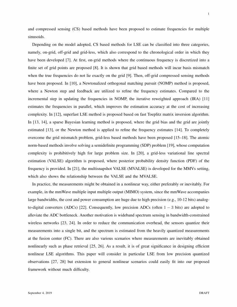
The pseudo linear measurement model is described as

y = A(θ)w + ε, (24)

where ε ∼ CN (ε; 0, diag(σ2)) and σ2 is known.

w p s p θ θ |p w s s 2; ,diag( )y A θ w σ

Fig. 1. The factor graph of (24) borrowed from [20].

For model (24), the factor graph is presented in Fig. 1. Given the pseudo measurements y and nuisance

parameters βw, the above joint PDF is

p(y,Ω;βw) ∝

(N∏i=1

p(θi)p(si)p(wi|si)

)p(y|θ,w), (25)

where p(y|θ,w) = CN (y; A(θ)w,Σ), and Σ = diag(σ2). Performing the type II maximum likelihood

(ML) estimation of the model parameters βw are still intractable. Thus variational approach where a given

structured PDF q(Ω|y) is used to approximate p(Ω|y) is adopted, where p(Ω|y) = p(y,Ω;βw)/p(y;βw)

and p(y;βw) =∫p(y,Ω;βw)dΩ. The variational Bayesian uses the Kullback-Leibler (KL) divergence

of p(Ω|y) from q(Ω|y) to describe their dissimilarity, which is defined as [53, p. 732]

KL(q(Ω|y)||p(Ω|y)) =

∫q(Ω|y) log

q(Ω|y)

p(Ω|y)dΩ. (26)

5The code that we have made available also provides the scalar EP.


9

In general, the posterior PDF q(Ω|y) is chosen from a distribution set to minimize the KL divergence.

The log model evidence ln p(y;βw) for any assumed PDF q(Ω|y) is [53, pp. 732-733]

ln p(y;βw) = KL(q(Ω|y)||p(Ω|y)) + L(q(Ω|y)), (27)

where

L(q(Ω|y)) = Eq(Ω|y)

[ln p(y,Ω;βw)

q(Ω|y)

]. (28)

For a given data y, ln p(y;βw) is constant, thus minimizing the KL divergence is equivalent to maximizing

L(q(Ω|y)) in (27). Therefore we maximize L(q(Ω|y)) in the sequel.

For the factored PDF q(Ω|y), the following assumptions are made:

• Given y, the frequencies θiNi=1 are mutually independent.

• The posterior of the binary hidden variables q(s|y) has all its mass at s, i.e., q(s|y) = δ(s− s).

• Given y and s, the frequencies and weights are independent.

As a result, q(Ω|y) can be factored as

q(Ω|y) =

N∏i=1

q(θi|y)q(w|y, s)δ(s− s). (29)

Due to the factorization property of (29), the frequency θ can be estimated from q(Ω|y) as [20]

θi = arg(Eq(θi|y)[ejθi ]), (30a)

ai = Eq(θi|y)[aN (θi)], i ∈ 1, ..., N, (30b)

where arg(·) returns the angle. For the given posterior PDF q(w|y, s), the mean and covariance estimates

of the weights are calculated as

w = Eq(w|y)[w], (31a)

Ci,j = Eq(w|y)[wiw∗j ]− wiw∗j , i, j ∈ 1, ..., N. (31b)

Given that q(s|y) = δ(s− s), the posterior PDF of w is

q(w|y) =

∫q(w|y, s)δ(s− s)ds = q(w|y, s). (32)

Let S be the set of indices of the non-zero components of s, i.e.,

S = i|1 ≤ i ≤ N, si = 1.

Analogously, we define S based on s. The model order is the cardinality of S, i.e.,

K = |S|.


10

Finally, the line spectral z =K∑k=1

a(θk)wk is reconstructed as

z =∑i∈S

aiwi.

The following procedure is similar to [21]. Maximizing L(q(Ω|y)) with respect to all the factors

is also intractable. Similar to the Gauss-Seidel method [54], L is optimized over each factor q(θi|y),

i = 1, . . . , N and q(w, s|y) separately with the others being fixed. Maximizing L(q(Ω|y);βw) (28) with

respect to the posterior approximation q(Ωd|y) of each latent variable Ωd, d = 1, . . . , N + 1 yields [53,

pp. 735, eq. (21.25)]

ln q(Ωd|y) = Eq(Ω\Ωd|y)[ln p(y,Ω)] + const, (33)

where the expectation is taken with respect to all the variables Ω except Ωd and the constant ensures

normalization of the PDF. In the ensuing three Subsections, we detail the procedures.

A. Inferring the Frequencies

For each i = 1, ..., N , we maximize L with respect to the factor q(θi|y). For i /∈ S, we have q(θi|y) =

p(θi). For i ∈ S, according to (33), the optimal factor q(θi|y) can be calculated as

ln q(θi|y) =Eq(Ω\θi|y) [ln p(y,Ω;βw)] + const, (34)

Substituting (30) and (31) in (34), one obtains

ln q(θi|y) = Eq(Ω\θi|y)[ln p(y,Ω;βw)] + const

=Eq(z\θi|y)[ln(p(θ)p(s)p(w|s)p(y|θ,w))] + const

= ln p(θi)− Eq(z\θi|y)[(y −ASwS)HΣ−1(y −ASwS)] + const

= ln p(θi) + <ηHi a(θi)+ const, (35)

where the complex vector ηi is given by

ηi = 2Σ−1

y −∑

l∈S\i

alwl

w∗i −∑

l∈S\i

alCl,i

, (36)

where “ ∼ i” denote the indices S excluding i, wS denotes the subvector of w by choosing the S rows

of w. The result is consistent with [20, eq. (17)] when the diagonal covariance matrix Σ reduces to the

scaled identity matrix. q(θi|y) is calculated to be

q(θi|y) ∝ p(θi)exp(<ηHi a(θi)). (37)

Since it is hard to obtain the analytical results (30b) for the PDF (37), q(θi|y) is approximated as a von

Mises distribution. For further details, please refer to [20, Algorithm 2: Heurestic 2].


11

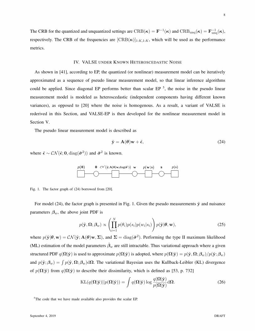
B. Inferring the Weights and Support

Next we keep q(θi|y), i = 1, ..., N fixed and maximize L w.r.t. q(w, s|y). Define the matrices J and

h as

Jij =

tr(Σ−1), i = j

aHi Σ−1aj , i 6= j

, i, j ∈ 1, 2, · · · , N, (38a)

h = AHΣ−1y, (38b)

where A = [a1, · · · , aN ]. According to (33), q(w, s|y) can be calculated as

ln q(w, s|y) = Eq(Ω\(w,s)|y) [ln p(y,Ω;βw)] + const

=Eq(θ|y)[

N∑i=1

ln p(si) + ln p(w|s) + ln p(y|θ,w)] + const

=− (wS − wS)HC−1S (wS − wS) + const, (39)

where

CS =

(JS +

I|S|

τ

)−1

, (40a)

wS = CShS . (40b)

It is worth noting that calculating CS and wS involves a matrix inversion. In the Appendix X-A, it is

shown that CS and wS can be updated efficiently.

From (29), the posterior approximation q(w, s|y) can be factored as the product of q(w|y, s) and

δ(s− s). According to the formulation of (39), for a given s, q(wS |y) is a complex Gaussian distribution,

and q(w|y; s) is

q(w|y; s) = CN (wS ; wS , CS)∏i 6∈S

δ(wi). (41)

Plugging the postulated PDF (29) in (28), one has

L(q(Ω|y); s) = Eq(Ω|y)

[p(y,Ω; s)

q(Ω|y)

]=Eq(Ω|y)[

N∑i=1

ln p(si) + ln p(w|s) + ln p(y|θ,w)− ln q(w|y)] + const

=− ln det(JS +1

τI|S|) + hH

S (JS +1

τI|S|)

−1hS + ||s||0 lnρ

1− ρ+ ||s||0 ln

1

τ+ const

, lnZ(s)|s=s (42)


12

Then we need to find s which maximizes lnZ(s), i.e.,

s = argmaxs

lnZ(s). (43)

The computation cost of enumerative method to find the globally optimal binary sequence s of (43) is

O(2N ), which is impractical for typical values of N . In Appendix X-A, a greedy iterative search strategy

similar to [20] is proposed. Since each step increases the objective function (which is bounded) and s

can take a finite number of values (at most 2N ), the method converges in a finite number of steps to

some local optimum. In general, numerical experiments show that O(K) steps is often enough to find

the local optimum.

Once s is updated as s′, the mean w′S′ and covariance C′S′ of the weights should be updated accordingly.

For the active case, w′S′ and covariance C′S′ are updated according to (85) and (84), while for the deactive

case, w′S′ and covariance C′S′ are updated according to (91) and (90).

C. Estimating the Model Parameters

After updating the frequencies and weights, the model parameters βw = ρ, τ are estimated via

maximizing the lower bound L(q(Ω|y);βw) for fixed q(Ω|y). Straightforward calculation shows that

L(q(Ω|y);βw) = Eq(Ω|y)

[ln p(y,Ω;βw)

q(Ω|y)

]=Eq(Ω|y)[

N∑i=1

ln p(si) + ln p(w|s)] + const

=||s||0 ln ρ+ (N − ||s||0) ln(1− ρ) + ||s||0 ln1

πτ− Eq(w|y)[

1

τwHSwS ] + const. (44)

Because

Eq(w|y)[wHSwS)] = Eq(w|y)[

∑i∈S

w∗iwi] = wHS wS + tr(CS),

we obtain

L(q(Ω|y);βw) = −1

τ[(wHS wS) + tr(CS)] + ||s||0(ln

ρ

1− ρ− lnτ) +N ln(1− ρ) + const.

Setting ∂L∂ρ = 0, ∂L

∂τ = 0, we have

ρ =||s||0N

,

τ =wHS wS + tr(CS)

||s||0. (45)


13

V. VALSE-EP ALGORITHM

In this section, the VALSE-EP algorithm is developed based on EP [40]. According to EP and the

factor graph presented in Fig. 2, the quantization model is iteratively reduced to a sequence of pseudo

unquantized models [41]. As a result, the original quantized LSE problem is decoupled into two modules:

the VALSE module named module A and the componentwise MMSE module named module B. The two

modules iteratively exchange the extrinsic information and refine their estimates.

Note that the factor graph shown in Fig. 2 only requires that p(y|z) =N∏n=1

p(yn|zn). As a result, it

is believed that VALSE-EP is very general and can have a wider implication to a range of nonlinear

identification issues in signal processing, such as phase retrieval y = |z + ε| in noncoherent channel

estimation [55], impulsive noise scenario y = z + ε where ε is the impulsive noise.

The detailed VALSE-EP is presented as follows.

m z z

mz z

z

(a)

(b)

p s |p w s w

θ p θ

s

module A

VALSE

MMSE y

module B

ext

Az

ext

Bz

ext

Av

ext

Bv

y A θ w ε

2,diag( )ε 0 σ

w

θ

( ) z A θ w |p y z

K

Fig. 2. Factor graph of the joint PDF (10) and the module of the VALSE-EP algorithm. Here the circle denotes the variable node,

and the square denotes the factor node. According to the dashed block diagram in Fig. 1 (a), the problem can be decomposed

as two modules in Fig. 1 (b), where module A corresponds to the standard linear model, and module B corresponds to the

componentwise MMSE estimation. Intuitively, the problem can be solved by iterating between the two modules, where module

A performs a variant of VALSE algorithm, and module B performs the componentwise MMSE estimation.

A. Componentwise MMSE module

The factor graph and the algorithm module are shown in Fig. 2. Specifically, in the tth iteration, let

mtδ→z(z) = CN (zext

A (t),diag(vextA (t))) denote the message transmitted from the factor node δ(z−Aw)

to the variable node z, which can be regarded as an extrinsic information from module A. According to


14

EP, the message mtz→δ(z) transmitted from the variable node z to the factor node δ(z −Aw) can be

calculated as [40]

mtz→δ(z) ∝

Proj[mtδ→z(z)p(y|z)]

mtδ→z(z)

,Proj[qtB(z)]

mtδ→z(z)

, (46)

where p(y|z) =∏Nn=1 p(yn|zn) and p(yn|zn) is (17), ∝ denotes identity up to a normalizing constant.

First, the posterior means and variances of z in module B can be obtained, i.e.,

zpostB (t) = E[z|qtB(z)], (47)

vpostB (t) = Var[z|qtB(z)], (48)

where E[·|qtB(z)] and Var[·|qtB(z)] are the mean and variance operations taken componentwise with

respect to the distribution ∝ qtB(z) and closed-form expression exists for quantized measurements [42].

As a result, Proj[qtB(z)] is

Proj[qtB(z)] = CN (z; zpostB (t),diag(vpost

B (t))). (49)

Substituting (49) in (46), the message mtz→δ(z) from the variable node z to the factor node δ(z−Ax)

is calculated as

mtz→δ(z) ∝

CN (z; zpostB (t),diag(vpost

B (t)))

CN (z; zextA (t),diag(vext

A (t)))∝ CN (z; zext

B (t),diag(vextB (t))), (50)

which can be viewed as the extrinsic information from module B and zextB (t) and vext

B (t) are [41]

vextB (t) =

(1

vpostB (t)

− 1

vextA (t)

)−1

, (51a)

zextB (t) = vext

B (t)

(zpost

B (t)

vpostB (t)

−zext

A (t)

vextA (t)

), (51b)

where denotes componentwise multiplication.

In addition, EM algorithm can be incorporated to learn the noise variance σ2 [59]. The posterior

distribution of z is approximated as (49). We compute the expected complete log-likelihood function

log p(y|z;σ2) + logmtδ→z(z) with respect to q(z|y;σ2(t)), and drop the irrelevant terms to have

Q(σ2;σ2(t)) = Eq(z|y;σ2(t))

[log p(y|z;σ2)

]. (52)

Then σ2 is updated as

σ2(t+ 1) = argmaxσ2

Q(σ2;σ2(t)). (53)

For the AWGN model

y = z + ε, (54)


15

where ε ∼ CN (ε; 0, σ2I), the posterior PDF q(z|y;σ2(t)) is

q(z|y;σ2(t)) = CN (z; zpostB (t), diag(vpost

B (t))). (55)

Substituting (55), (54) and (52) in (53), the noise variance σ2 is estimated as

σ2(t+ 1) =‖y − zpost

B (t)‖2 + 1TvpostB (t)

M. (56)

For arbitrary p(y|z) including the quantized case, we also obtain an approximate update equation. From

the definition of mz→δ(z) and z = A(θ)x, we obtain a pseudo measurement model

y(t) = z + ε(t), (57)

where y(t) = zextB (t), ε(t) ∼ CN (ε(t); 0, diag(σ2(t))) and σ2(t) = vext

B (t). The noise variance σ2 is

updated as [51]

σ2(t+ 1) =‖y(t)− zpost

B (t)‖2 + 1TvpostB (t)

M. (58)

Note that (56) is a special case of (58), as for the AWGN model (54), y = y is proved later according

to (75a) and (76a).

B. VALSE module

According to (50), the message mtz→δ(z) (nonGaussian likelihood) transmitted from the variable node

z to the factor node δ(z−Ax) is iteratively approximated as a Gaussian distribution (Gaussian likelihood),

and the factor graph is shown in Fig. 3 (a). Based on the definition of the factor node δ(z−Ax) and the

message mtz→δ(z) transmitted from the variable node z to the factor node δ(z −Aw), a pseudo linear

measurement model

y(t+ 1) = A(θ)w + ε(t+ 1), (59)

is obtained, where ε(t+ 1) ∼ CN (ε(t+ 1); 0,diag(σ2(t+ 1))), and

y(t+ 1) = zextB (t), (60)

σ2(t+ 1) = vextB (t). (61)

As a result, the pseudo factor graph Fig. 3 (b) is obtained and is equivalent to Fig. 1. In Section IV, a

variant of VALSE is rederived. Here we run the VALSE in a single iteration and output the approximated

posterior PDF q(wS |y) and q(θ|y).


16

m z z

mz z

z

(a)

(b)

p s |p w s w

θ p θ

s

w p s p θ θ |p w s s

z A θ w 2; ,diag( ) y z σ

2; ,diag( ) y A θ w σ

Fig. 3. Two equivalent factor graphs of the joint PDF (25). The dashed square denotes the pseudo factor node.

C. From VALSE module to MMSE module

According to the approximated posterior PDF q(wS |y) and q(θ|y), we calculate the message mt+1δ→z(z)

as

mt+1δ→z(z) ∝

Proj[∫q(wS |y)δ(z−AS(θ)wS)q(θ|y)dwSdθ]

mtz→δ(z)

,Proj[qt+1

A (z)]

mtz→δ(z)

. (62)

According to (62), the posterior means and variances of z averaged over qt+1A (z) in module A are

zpostA (t+ 1) = ASwS , (63)

vpostA (t+ 1) = diag(ASCSAH

S) +

(wHS

wS1N − |AS |2|wS |

2)

+[tr(CS)1N − |AS |

2diag(CS)], (64)

where details of (64) are postponed to Appendix X-B. Thus Proj[qt+1A (z)] is

Proj[qt+1A (z)] = CN (z; zpost

A (t+ 1),diag(vpostA (t+ 1))). (65)

According to (62), mt+1δ→z(z) is calculated to be

mt+1δ→z(z) = CN (z; zext

A (t+ 1),diag(vextA (t+ 1))), (66)

where the extrinsic means zextA (t+ 1) and variances vext

A (t+ 1) are given by [41]

1

vextA (t+ 1)

=1

vpostA (t+ 1)

− 1

σ2w(t+ 1)

, (67)

zextA (t+ 1) = vext

A (t+ 1)

(zpost

A (t+ 1)

vpostA (t+ 1)

− y(t+ 1)

σ2w(t+ 1)

), (68)

and we input them to module B. The algorithm iterates until convergence or the maximum number of

iterations is reached. The VALSE-EP algorithm is summarized as Algorithm 1.


17

Algorithm 1 VALSE-EP algorithm1: Set the number of iterations T and implement the initialization in Subsection V-D.

2: for t = 1, · · · , T do

3: Update J (38a) and h (38b) using y(t) and σ2(t).

4: Update s, wS and CS (Section IV-B).

5: Update ρ, τ (45) (Section IV-C).

6: Update ηi and ai for all i ∈ S (Section IV-A).

7: Calculate the posterior means zpostA (t) (63) and variances vpost

A (t) (64).

8: Compute the extrinsic mean and variance of z as vextA (t) (67), zext

A (t) (68).

9: Compute the post mean and variance of z as zpostB (t) (47), vpost

B (t) (48).

10: Compute the extrinsic mean and variance of z as zextB (t) (51b) and vext

B (t) (51a), and set σ2(t+1) =

vextB (t) and y(t+ 1) = zext

B (t). Implement EM to estimate the noise variance as σ2(t+ 1) (58).

11: end for

12: Return θ, w, z and K.

D. Initialization

The initialization of VALSE-EP is presented. First, the additive quantization noise model (AQNM)

[56]

yq = z + ε + εq, (69)

is adopted, where the output levels yq are the midpoints of the quantization interval, εq is the quan-

tization error. First, the noise variance σ2 is initialized. For n′

= 1, · · · , N − 1, we calculate γn′ =

1N

∑(k′ ,l′ )∈Υ

n′ yk′y∗

l′with Υn′ = (k′

, l′)|1 ≤ k′

, l′ ≤ N −1, k

′ − l′ = n′. We use γ to build a Toeplitz

estimate of E[yqyHq ]. Then, we initialize σ2 with the average of the lower quarter of the eigenvalues of

the Toeplitz matrix (ignoring the quantization noise). Typically, it is found that setting vextA ranging from

1 ∼ 102 works well. Here we initialize zextA = 0 and vext

A = 10. After performing the MMSE estimation in

module B, y = zextB and σ2 = vext

B are obtained. Given that E[ydiag(σ−2)yH] = N+ρNτtr(diag(σ−2)),

we set ρ = 0.5 and let τ = (ydiag(σ−2)yH−N)/(ρNtr(diag(σ−2))). Then in step i, when the first i−1

PDFs of the frequencies are initialized, the estimates wi−1k=1 and the residual yr

i−1 = y −∑i−1

k=1 akwk

are obtained. Then initialize q(θi|yri−1) ∝ exp

(|yri−1diag(σ−2)a(θ)|2/N

)and project it as a von Mises

distribution and compute ai.


18

E. Computation Complexity

From Algorithm 1, it can be seen that VALSE-EP involves the componentwise MMSE operation and

VALSE. For the componentwise MMSE operation, the computation complexity is O(NK). As for the

VALSE, the complexity per iteration is dominated by the two steps: the maximization of lnZ(s) and the

approximations of the posterior PDF q(θi|y) by mixtures of von Mises PDFs. This work approximates

the posterior PDF q(θi|y) by Heuristic 2 in [20, Algorithm 2]. Thus the complexity of the two steps are

O(NK3) and O(N2) [20]. Therefore, the complexity of VALSE-EP is comparable to that of VALSE.

VI. RELATIONSHIP BETWEEN VALSE-EP AND VALSE UNDER UNQUANTIZED SETTING

Before revealing the relation between VALSE-EP and VALSE under unquantized setting, the following

properties are revealed.

Property 1 The noise variance estimate in VALSE can be equivalently derived in EM step.

PROOF In [20], the noise variance is estimated as (reformulated as our notation)

σ2VA(t+ 1) =

1

N‖y −

∑i∈S

aiwi‖22 +1

Ntr(J

′

SCS

)+∑i∈S

|wi|2(1− ‖ai‖22/N), (70)

where J′

ii = N and J′

ij = aHi aj . According to EM, the noise variance σ2(t+ 1) in module A should be

updated as (replacing zpostB (t) and vpost

B (t) with zpostA (t) and vpost

A (t) in (56), respectively)

σ2(t+ 1) =‖y − zpost

A (t)‖2 + 1TvpostA (t)

N. (71)

Substituting zpostA (t) (63) and vpost

A (t) (64) in (71) and utilizing J′

= AHA+NIN −diag(diag(AHA)),

one can show that σ2(t+ 1) = σ2VA(t+ 1).

Property 1 reveals that the noise variance estimates of both VALSE-EP and VALSE can be derived

via the EM step. For the VALSE algorithm, the noise variance estimate of the EM step is performed in

module A, while for VALSE-EP, the noise variance estimate of the EM step is performed in module B.

In the following text, the relationships between the posterior means and variances of VALSE and that of

VALSE-EP are derived.

Property 2 The relationships between the posterior means zpostB (t) and variances vpost

B (t) of z in module

B and the posterior means zpostA (t) and variances vpost

A (t) of z in module A are

1

vpostB (t+ 1)

=1

vpostA (t+ 1)

− 1

σ2(t)+

1

σ2(t+ 1), (72a)

zpostB (t+ 1)

vpostB (t+ 1)

=zpost

A (t+ 1)

vpostA (t+ 1)

− y

(1

σ2(t)− 1

σ2(t+ 1)

). (72b)


19

PROOF For the tth iteration, let the extrinsic means and variances of z from module A be zextA (t) and

vextA (t) (Step 8 in Algorithm 1), and the noise variance be σ2(t). The posterior variances (48) and means

(47) of z are

1

vpostB (t)

=1

vextA (t)

+1

σ2(t), (73a)

zpostB (t)

vpostB (t)

=zext

A (t)

vextA (t)

+y

σ2(t). (73b)

Then the extrinsic means and variances of z from module B zextB (t) and vext

B (t) are

1

vextB (t)

=1

vpostB (t)

− 1

vextA (t)

, (74a)

zextB (t)

vextB (t)

=zpost

B (t)

vpostB (t)

−zext

A (t)

vextA (t)

. (74b)

According to (73) and (74), one has

zextB (t) = y, (75a)

vextB (t) = σ2(t)1. (75b)

In addition, EM is implemented to update σ2 as σ2(t+ 1). By setting

y(t+ 1) = zextB (t), (76a)

σ2(t+ 1) = vextB (t) = σ2(t)1, (76b)

we run the VALSE (noise variance aware) algorithm, and calculate zpostA (t+ 1) and vpost

A (t+ 1). Then

zextA (t+ 1) and vext

A (t+ 1) are updated as

1

vextA (t+ 1)

=1

vpostA (t+ 1)

− 1

σ2(t+ 1), (77a)

zextA (t+ 1)

vextA (t+ 1)

=zpost

A (t+ 1)

vpostA (t+ 1)

− y(t+ 1)

σ2(t+ 1). (77b)

According to (73), (75), (76) and (77), (72) is obtained.

According to Property 2, vpostB (t + 1) = vpost

A (t + 1) and zpostB (t + 1) = zpost

A (t + 1) holds when

σ2(t) = σ2(t + 1), which means that the noise variance is a constant during the iteration. Combing

Property 1 and Property 2, it is concluded that in the unquantized setting VALSE-EP is equivalent to

VALSE when the noise variance is known, i.e., the noise variance estimation step is removed. In general,

VALSE-EP is not exactly equivalent to VALSE even in the unquantized setting.


20

VII. NUMERICAL SIMULATION

In this section, numerical experiments are conducted to evaluate the performance of the proposed

VALSE-EP algorithm. In addition, for performance comparison in the quantized setting, the AQNM is

adopted and yq (69) is directly input to the VALSE to perform estimation. Furthermore, VALSE-EP is

also compared with VALSE in unquantized setting.

A. Simulation Setup

The frequencies are randomly drawn such that the minimum wrap around distance is greater than

2π/N . The noninformative prior, i.e., p(θi) = 1/(2π), i = 1, · · · , N , is used for both VALSE and

VALSE-EP algorithm. The magnitudes of the weight coefficients are drawn i.i.d. from a Gaussian

distribution N (1, 0.04), and the phases are drawn i.i.d. from a uniform distribution between [−π, π].

For multi-bit quantization, a uniform quantizer is adopted and the quantization interval is restricted to

[−3σz/√

2, 3σz/√

2], where σ2z is the variance of z. In our setting, it can be calculated that σ2

z ≈ K. For

one-bit quantization, zero is chosen as the threshold. The SNR is defined as SNR = 20log(||A(θ)w||2/||ε||2).

Both VALSE and VALSE-EP stop at iteration t if ‖z(t)− z(t− 1)‖2/‖z(t)‖2 < 10−6 or the number of

iterations exceeds 1000.

The signal estimation error NMSE(z), the frequency estimation error MSE(θ) and the correct model

order estimation probability P(K = K) are used to characterize the performance. The normalized MSE

(NMSE) of signal z (for unquantized and multi-bit quantized system) and MSE of θ are defined as

NMSE(z) , 10log(||z−z||22/||z||22) and MSE(θ) , 10log(||θ−θ||22), respectively. Please note that, due

to magnitude ambiguity, it is impossible to recover the exact magnitude of wk from one-bit measurements

in the noiseless scenario. Thus for one-bit quantization, the debiased NMSE of the signal defined as

dNMSE(z) , minc

10 log(‖z∗ − cz‖22/‖z∗‖22) is calculated. As for the frequency estimation error, we

average only the trials in which all those algorithms estimate the correct model order. All the results are

averaged over 500 Monte Carlo (MC) trials unless stated otherwise. The MSE of the frequency estimation

is calculated only when the model order is correctly estimated.

At first, an experiment is conducted to show that VALSE-EP is able to suppress the harmonics coming

from the quantized data. The parameters are set as follows: N = 100, K = 2 and the true frequencies

are θ = [−1, 2]T. The results are shown in Fig. 4 for SNR = 0 dB, SNR = 20 dB and SNR = 40

dB. As stated in [57], the one-bit data consists of plentiful harmonics including self-generated and cross-

generated harmonics. especially at high SNR. For low SNR scenario (SNR = 0 dB), both VALSE and

VALSE-EP estimate the model order successfully. For medium (SNR = 20 dB) and high SNR (SNR = 40

dB) scenario, VALSE overestimates the model order, outputs the fundamental (true) frequency and the


21

-1.5

-1

-0.5

0

SNR=0 dB

-3 -2 -1 0 1 2 3

TrueVALSEVALSE-EP

(a) (b)

-25

-20

-15

-10

-5

0

SNR=40 dB

-3 -2 -1 0 1 2 3

(c)

Fig. 4. A typical reconstruction results of VALSE-EP and VALSE under 1 bit quantization at SNR = 0 dB, SNR = 20 dB

and SNR = 40 dB. The normalized amplitudes wnld , w/(maxi|wi|) are plotted.

self-generated and cross-generated harmonics. For example, the 3rd order harmonics corresponding to

W(−θ1 − 2θ2) ≈ −3, W(−θ1 + 2θ2) ≈ −1.28, W(2θ1 − θ2) ≈ 2.29, W(−2θ1 − θ2) = 0, the 5th

order harmonics corresponding to W(−4θ1 + θ2) ≈ −0.28, W(5θ1) ≈ 1.28, W(−2θ1 + 3θ2) ≈ 1.72,

W(2θ1 + 3θ2) ≈ −2.28, the 7th order harmonic W(−3θ1 + 4θ2) ≈ −1.57, are estimated for SNR = 20

dB. While, VALSE-EP estimates the model order correctly for both SNR = 20 dB and SNR = 40 dB,

demonstrating the effectiveness of suppressing the harmonics.

For the ensuing subsections, four numerical experiments with synthetic data and one with real data are

conducted to demonstrate the excellent performance of VALSE-EP under quantizied setting, compared

to VALSE.

B. NMSE of the Line Spectral versus Iteration

The NMSEs of the reconstructed line spectral versus the iteration are investigated and results are shown

in Fig. 5. Note that both VALSE-EP and VALSE converge in tens of iterations. For low SNR scenario

(SNR = 0 dB), VALSE-EP and VALSE are comparable. As SNR increases, the performance gap between


22

1 2 3 4 5 6 7 8 9 10 11 12 13 14 15 16 17 18 19 20Iteration

-14

-12

-10

-8

-6

-4

-2

SNR=0 dB

1 bit VALSE2 bit VALSE3 bit VALSE

bit VALSE

1 bit VALSE-EP2 bit VALSE-EP3 bit VALSE-EP

bit VALSE-EP

(a)

1 2 3 4 5 6 7 8 9 10 11 12 13 14 15 16 17 18 19 20Iteration

-35

-30

-25

-20

-15

-10

-5

SNR=20 dB

(b)

1 2 3 4 5 6 7 8 9 10 11 12 13 14 15 16 17 18 19 20Iteration

-60

-50

-40

-30

-20

-10

0

SNR=40 dB

(c)

Fig. 5. The NMSE of the LSE of the VALSE-EP versus the number of iterations under SNR = 0 dB, SNR = 20 dB, SNR = 40

dB, respectively. Here N = 100 and K = 3.

VALSE-EP and VALSE increases under quantized settings. Besides, the performance of the VALSE-EP

improves as SNR increases, especially for higher bit-depth. In contrast, for 1 bit quantization, VALSE

works well under low SNR scenario, and degrades as SNR increases. As the bit-depth increases, the

performances of the VALSE-EP and VALSE improve and approach to the unquantized setting.

C. Estimation versus SNR

The performance of the VALSE-EP versus SNR is investigated and the results are plotted in Fig. 6.

For the signal reconstruction and model order estimation probability, Fig. 6(a) and 6(b) show that for

1 bit and 2 bit quantization, as SNR increases, the performances of VALSE first improve, and then

degrade, while the performances of VALSE-EP always improve and are better than VALSE. A surprising

phenomenon is that VALSE-EP under 2 bit quantization achieves the highest success rate of model order

estimation and approaches to the CRB firstly. As the SNR continuous to increase, VALSE-EP deviates a

little away from CRB under 1 bit and 2 bit quantization, while in the unquantized setting, both VALSE

and VALSE-EP approach to the CRB asymptotically.


23

0 5 10 15 20SNR (dB)

-35

-30

-25

-20

-15

-10

-5

(a)

0 5 10 15 20SNR (dB)

0

0.2

0.4

0.6

0.8

1

(b)

0 5 10 15 20SNR (dB)

-70

-60

-50

-40

-30

-20

-10

0 1 bit VALSE2 bit VALSE

bit VALSE

1 bit VALSE-EP2 bit VALSE-EP

bit VALSE-EP

1 bit CRB2 bit CRB

bit CRB

(c)

Fig. 6. Performance versus SNR for N = 100 and K = 3: (a) NMSE of the reconstructed signal; (b) success rate of model

order estimation; (3) MSE of frequency estimation.

D. Estimation versus Number of Measurements N

The performances of both VALSE-EP and VALSE versus the number of measurements N are examined

and results are shown in Fig. 7. For both algorithms, the signal reconstruction error decreases as the

number of measurements N increases. It can be seen that VALSE-EP works better than VALSE under

1 bit and 2 bit quantization. As N increases, the success rate of model order estimation of VALSE

first increases and then decreases under 1 bit quantization. In contrast, the success rate of model order

estimation of VALSE-EP increases and even exceed the VALSE and VALSE-EP under unquantized setting

for N = 100. As for the frequency estimation error, VALSE-EP approaches to the CRB quickly than

VALSE under quantized setting.

E. Estimation versus Number of Spectral K

The performance of VALSE-EP is investigated with respect to the number of spectral K, and results

are presented in Fig. 8. For the signal reconstruction error and success rate of model order estimation,

the performances of all algorithms degrade as K increases, except that VALSE under 1 bit quantization,

which first improves and then degrades. For the frequency estimation error, as K increases, VALSE


24

40 60 80 100 120-25

-20

-15

-10

-5

(a)

40 60 80 100 1200

0.2

0.4

0.6

0.8

1

(b)

40 60 80 100 120-60

-50

-40

-30

-20

-10

0 1 bit VALSE2 bit VALSE

bit VALSE


bit VALSE-EP

1 bit CRB2 bit CRB

bit CRB

(c)

Fig. 7. The performance of VALSE-EP versus the number of measurements N for SNR = 10 dB and K = 3: (a) NMSE of

the reconstructed signal; (b) success rate of model order estimation; (3) MSE of frequency estimation.

degrades quickly and deviates far way from CRB when K ≥ 4 under 1 bit quantization. When K ≤ 6,

VALSE-EP is always close to the CRB under 1 bit quantization. As K continues to increase, the frequency

estimation error of VALSE-EP begin to deviate far way from CRB.

F. Real Data

The performance of VALSE-EP is evaluated with real data collected at sea, which was collected on

a HLA (part of the Shark array) during the Shallow Water 2006 (SW06) experiment on August 5 and

6, 2006 [58]. The array had 32 elements uniformly spaced at d = 15 m (design frequency f = 50 Hz,

thus the wavelength λ is λ = c/f = 1500/50 = 30 m and d = λ/2). The first 1000 snapshots (8494

snapshots in total) are used. The source depths are estimated to be around 12 m. For the DOA problem,

θi = −2πd/λ sinϕi = −π sinϕi, where ϕiKi=1 denote the DOAs. The variance of the real data is

calculated to be 0.0136, which is used to design the 2 bit quantizer.

The synthesized posterior PDF of frequencies 1/|S||S|∑i=1

q(θi|Y)|θi=−π sinϕibased on the data from one

of the oblique runs is presented. In [58], it is stated that the towed source signal is at sinϕ1 ≈ 0.1, and

a signal (the interferer source) near the endfire direction (sinϕ2 ≈ −0.9) is assumed to be from a ship


25

3 4 5 6 7 8K

-25

-20

-15

-10

(a)

3 4 5 6 7 8K

0

0.2

0.4

0.6

0.8

1

(b)

3 4 5 6 7 8K

-60

-50

-40

-30

-20

-10

01 bit VALSE2 bit VALSE

bit VALSE


bit VALSE-EP

1 bit CRB2 bit CRB

bit CRB

(c)

Fig. 8. The performance of VALSE-EP versus the number of spectrum K for N = 160 and SNR = 10 dB.

(The existence of this ship is unknown). For unquantized setting, Fig.9(c) and Fig. 9(f) are consistent

with the results obtained in [58]. While when the data is heavily quantized into 1 bit and 2 bit, the towed

source signal is estimated accurately and the interferer source disappears for VALSE-EP. In contrast, the

towed source signal are estimated accurately for VALSE algorithm, with an additional false source signal

corresponding to the third order harmonic −3× (−π sinϕ1) ≈ 0.3π (located at −0.3 in Fig. 9(a)) of the

fundamental frequency −π sinϕ1 ≈ −0.1π.

VIII. CONCLUSION

In this paper, a VALSE-EP algorithm is proposed to deal with the fundamental LSE problem from

quantized samples. The VALSE-EP is one kind of low-complexity grid-less algorithm which iteratively

refines the frequency estimates, automatically estimates the model order, and learns the parameters of

the prior distribution and noise variance. Importantly, VALSE-EP provides the uncertain degrees of the

frequency estimates from quantized samples. Substantial numerical experiments are conducted to show

the excellent performance of the VALSE-EP, including on a real data set.


26

1 bit VALSE

-0.9 -0.3 0.1 0.5 1

0

50

100

150

Tim

e(se

c)

-10

-5

0

5

10

15

20

(a)

2 bit VALSE

-0.9 -0.3 0.1 0.5 1

0

50

100

150

Tim

e(se

c)

-10

-5

0

5

10

15

20

(b)

bit VALSE

-0.9 -0.3 0.1 0.5 1

0

50

100

150

Tim

e(se

c)

-10

-5

0

5

10

15

20

(c)

1 bit VALSE-EP

-0.9 -0.3 0.1 0.5 1

0

50

100

150T

ime(

sec)

-10

-5

0

5

10

(d)

2 bit VALSE-EP

-0.9 -0.3 0.1 0.5 1

0

50

100

150

Tim

e(se

c)

-10

-5

0

5

10

15

(e)

bit VALSE-EP

-0.9 -0.3 0.1 0.5 1

0

50

100

150

Tim

e(se

c)

-10

-5

0

5

10

15

20

(f)

Fig. 9. The synthesized posterior PDF of sinϕ for real data.

IX. ACKNOWLEDGEMENT

The authors acknowledge the editor and the four anonymous reviewers for valuable comments and

suggestions on this work.


27

X. APPENDIX

A. Finding the local maximum of lnZ(s)

A greedy iterative search strategy similar to [20] is adopted to find a local maximum of lnZ(s). We

proceed as follows: In the pth iteration, the kth test sequence tk which flips the kth element of s(p) is

obtained. Then ∆(p)k = lnZ(tk) − lnZ(sp) is calculated for each k = 1, · · · , N . If ∆

(p)k < 0 holds for

all k, the algorithm is terminated and s is set as s(p), otherwise tk corresponding to the maximum ∆(p)k

is chosen as s(p+1) in the next iteration.

When k 6∈ S, that is, sk = 0, we activate the kth component of s by setting sk = 1. Now, S ′ = S∪k.

∆k = lnZ(s′)− lnZ(s)

= ln det(JS +1

τI|S|)− ln det(JS′ +

1

τI|S′|)

+ lnρ

1− ρ+ ln

1

τ+ hH

S′(JS′ +1

τI|S′|)

−1hS′ − hHS (JS +

1

τI|S|)

−1hS . (78)

Let jk be jk = [Jik|i ∈ S]T. By using the block-matrix determinant formula, one has

ln(det(JS′ +1

τI|S′|)) = ln det(JS +

1

τI|S|) + ln

(tr(Σ−1) +

1

τ− jH

k (JS +1

τI|S|)

−1jk

), (79)

By the block-wise matrix inversion formula, one has

hHS′(JS′ +

1

τI|S′|)

−1hS′ = hHS (JS +

1

τI|S|)

−1hS +ξ∗ξ

tr(Σ−1) + 1τ − jH

k (JS + 1τ I|S|)−1jk

, (80)

where ξ = hk − jHk (JS + 1

τ I|S|)−1hS . Plugging (79) and (80) in (78), and let

vk =

(tr(Σ−1) +

1

τ− jH

k (JS +1

τI|S|)

−1jk

)−1

and

uk = vk

(hk − jH

k (JS +1

τI|S|)

−1hS

), (81)

∆k can be simplified as

∆k = lnvkτ

+|uk|2

vk+ ln

ρ

1− ρ. (82)

Given that s is changed into s′, the mean w′S′ and covariance C′S′ of the weights can be updated from

(40), i.e.,

C′S′ = (JS′ +1

τI|S′|)

−1, (83a)

w′S′ = CS′hS′ . (83b)


28

In fact, the matrix inversion can be avoided when updating w′S′ and CS′ . It can be shown thatC′S′\k c′k

c′Hk C ′kk

= (JS′ +1

τI|S′|)

−1

=

CS 0

0 0

+ vk

CSjk

−1

CSjk

−1

H

=

CS + vkCSjk(CSjk)H −vkCSjk

−vk(CSjk)H vk

(84)

C′S′ is obtained if c′k, c′Hk and C ′kk are inserted appropriately in C′S′\k, andw′S′\k

w′k

= CS′hS′

=

CShS + vkCSjkjHk CShS − vkCSjkhk

−vkjHk CShS + vkhk

=

CShS − ukCSjkuk

. (85)

From (85) and (84), one can see that after activating the kth component, the posterior mean and variance

of wk are uk and vk, respectively.

For the deactive case with sk = 1, s′k = 0 and S ′ = S\k, ∆k = lnZ(s′)− lnZ(s) is the negative

of (82), i.e.,

∆k = − lnvkτ− |uk|

2

vk− ln

ρ

1− ρ. (86)

Similar to (84), the posterior mean and covariance update equation from S ′ to S case can be rewritten

as C′S′ 0

0 0

+ vk

C′S′jk

−1

C′S′jk

−1

H

=

CS\k ck

cHk Ckk

, (87)

and w′S′ − ukC′S′jk

uk

=

C′S′hS′ − ukC′S′jk

uk

=

wS\k

wk

, (88)

where ck,0 denotes the column of CS,0 corresponding to the kth component. According to (87) and (88),

one has

C′S′ + vkC′S′jkj

Hk C′S′ = CS\k, (89a)

−vkC′S′jk = ck (89b)

vk = Ckk, (89c)

w′S′ − ukC′S′jk = wS\k, (89d)

uk = wk. (89e)


29

Thus, C′S′ can be updated by substituting (89b) and (89c) in (89a), i.e.,

C′S′ = CS\k − vkC′S′jkjHk C′S′ = CS\k −

ckcHk

Ckk. (90)

Similarly, w′S′ can be updated by substituting (89b) and (89e) in (89d), i.e.,

w′S′ = ukC′S′jk + wS\k = wS\k −

wk

Ckkck. (91)

According to vk = Ckk (89c) and uk = wk (89e), ∆k (86) can be simplified as

∆k = − lnCkkτ− |wk|

2

Ckk− ln

ρ

1− ρ. (92)

B. Calculating the post variance vpostA (64) of z

Now we calculate the variance of zn given q(wS |y) and q(θ|y). Let bTn = [ej(n−1)θ1 , ej(n−1)θ2 , · · · , ej(n−1)θK ]

be the nth row of AS . Then zn = bTnwS . The variance is

Var[zn] = E[|zn|2]− |E[zn]|2 = E[|bTnwS |

2]− |E[bTnwS ]|2

= tr[(CS + wSwH

S)E[b∗nb

Tn ]]− |bT

n wS |2. (93)

where

E[b∗nbTn ] = b∗nb

Tn + diag

(1K − |bn|

2). (94)

Substituting (94) in (93), one obtains (64).

REFERENCES

[1] VALSE-EP code, https://github.com/RiverZhu/VALSE-EP

[2] W. Bajwa, A. Sayeed, and R. Nowak, “Compressed channel sensing: A new approach to estimating

sparse multipath channels,” Proc. IEEE, vol. 98, pp. 1058-1076, Jun. 2010.

[3] B. Ottersten, M. Viberg and T. Kailath, “Analysis of subspace fitting and ML techniques for parameter

estimation from sensor array data,” IEEE Trans. Signal Process., vol. 40, pp. 590-600, 1992.

[4] P. Stoica and R. L. Moses, Spectral Analysis of Signals. Upper Saddle River, NJ, USA: Prentice-Hall,

2005.

[5] R. Schmidt, “Multiple emitter location and signal parameter estimation,” IEEE Trans. Antennas

Propag., vol. 34, no. 3, pp. 276-280, 1986.

[6] R. Roy and T. Kailath, “ESPRIT-estimation of signal parameters via rotational invariance techniques,”

IEEE Trans. Acoust., Speech, Signal Process., vol. 37, no. 7, pp. 984-995, 1989.

[7] Z. Yang Z, J. Li, P. Stoica P and Xie L, “Sparse methods for direction-of-arrival estimation,” Academic

Press Library in Signal Processing, vol. 7, pp. 509-581, 2018.


30

[8] D. Malioutov, M. Cetin and A. Willsky, “A sparse signal reconstruction perspective for source

localization with sensor arrays,” IEEE Trans. Signal Process., vol. 53, no. 8, pp. 3010-2022, 2005.

[9] Y. Chi, L. L. Scharf, A. Pezeshki and R. Calderbank, “Sensitivity of basis mismatch to compressed

sensing,” IEEE Trans. on Signal Process., vol. 59, pp. 2182 - 2195, 2011.

[10] B. Mamandipoor, D. Ramasamy and U. Madhow, “Newtonized orthogonal matching pursuit:

Frequency estimation over the continuum,” IEEE Trans. Signal Process., vol. 64, no. 19, pp. 5066-

5081, 2016.

[11] J. Fang, F. Wang, Y. Shen, H. Li and R. S. Blum, “Superresolution compressed sensing for line

spectral estimation: an iterative reweighted approach,” IEEE Trans. Signal Process., vol. 64, no. 18,

pp. 4649-4662, 2016.

[12] T. L. Hansen, B. H. Fleury and B. D. Rao, “Superfast line spectral estimation,” IEEE Trans. Signal

Process., vol. 66, no. 10, pp. 2511-2526, 2018.

[13] L. Hu, J. Zhou, Z. Shi and Q. Fu, “A fast and accurate reconstruction algorithm for compressed

sensing of complex sinusoids,” IEEE Trans. Signal Process., vol. 61, no. 22, pp. 5744-5754, 2013.

[14] L. Hu, Z. Shi, J. Zhou and Q. Fu, “Compressed sensing of complex sinusoids: An approach based

on dictionary refinement,” IEEE Trans. Signal Process., vol. 60, no. 7, pp. 3809-3822, 2012.

[15] G. Tang, B. Bhaskar, P. Shah and B. Recht, “Compressed sensing off the grid,” IEEE Trans. Inf.

Theory, vol. 59, no. 11, pp. 7465-7490, 2013.

[16] Z. Yang and L. Xie, “On gridless sparse methods for line spectral estimation from complete and

incomplete data,” IEEE Trans. Signal Process., vol. 63, no. 12, pp. 3139-3153, 2015.

[17] Y. Li and Y. Chi, “Off-the-grid line spectrum denoising and estimation with multiple measurement

vectors,” IEEE Trans. Signal Process., vol. 64, no. 5, pp. 1257-1269, 2016.

[18] Z. Yang, L. Xie and C. Zhang, “A discretization-free sparse and parametric approach for linear array

signal processing,” IEEE Trans. Signal Process., vol. 62, no. 19, pp. 4959-4973, 2014.

[19] S. Boyd and L. Vandenberghe, Convex Optimization, Cambridge University Press, 2004.

[20] M. A. Badiu, T. L. Hansen and B. H. Fleury, “Variational Bayesian inference of line spectra,” IEEE

Trans. Signal Process., vol. 65, no. 9, pp. 2247-2261, 2017.

[21] J. Zhu, Q. Zhang, P. Gerstoft, M. A. Badiu and Z. Xu, “Grid-less variational Bayesian line spectral

estimation with multiple measurement vectors,” Signal Process., vol. 61, pp. 155-164, 2019.

[22] S. Rangan, T. S. Rappaport and E. Erkip, “Millimeter-wave cellular wireless networks: potentials

and challenges,” Proc. IEEE, vol. 102, no. 3, pp. 366-385, 2014.

[23] O. Mehanna and N. Sidiropoulos, “Frugal sensing: Wideband power spectrum sensing from few

bits,” IEEE Trans. on Signal Process., vol. 61, no. 10, pp. 2693-2703, 2013.


31

[24] Y. Chi and H. Fu, “Subspace learning from bits,” IEEE Trans. on Signal Process., vol. 65, no. 17,

pp. 4429-4442, Sept 2017.

[25] P. Schniter and S. Rangan, “Compressive phase retrieval via generalized approximate message

passing,” IEEE Trans. Signal Process., vol. 63, no. 4, pp. 1043-1055, 2015.

[26] S. Wang, L. Zhang and X. Jing, “Phase retrieval motivated nonlinear MIMO communication with

magnitude measurements,” IEEE Trans. Wireless Commun., vol. 16, no. 8, pp. 5452-5466, 2017.

[27] F. Li, J. Fang, H. Li and L. Huang, “Robust one-bit Bayesian compressed sensing with sign-flip

errors,” IEEE Signal Process. Lett., vol. 22, no. 07, 2015.

[28] J. Fang, Y. Shen, L. Yang and H. Li, “Adaptive one-bit quantization for compressed sensing,” Signal

Process., vol. 125, pp. 145-155, 2016.

[29] G. Franceschetti, V. Pascazio, G. Schirinzi, “Processing of signum coded SAR signal: theory and

experiments,” IEE Proceedings F - Radar and Signal Processing, vol. 138, no. 3, pp. 192-198, 1991.

[30] C. Gianelli, L. Xu, J. Li, P. Stoica, “One-bit compressive sampling with time-varying thresholds

for sparse parameter estimation,” IEEE Sensor Array and Multichannel Signal Processing Workshop

(SAM), Rio de Janerio, Brazil, July 10-13, 2016.

[31] J. Li, M. M. Naghsh, S. J. Zahabi, M. M. Hashemi, “compressive radar sensing via one-bit sampling

with time-varying thresholds,” 50th Asilomar Conference on Signals, Systems and Computers, Pacific

Grove, CA, USA, 6-9 Nov. 2016.

[32] K. Yu, Y. Zhang, M. Bao, Y. Hu and Z. Wang, “DOA estimation from one-bit compressed array

data via joint sparse representation,” IEEE Signal Process. Lett., vol. 23, no. 9, pp. 1279-1283, 2016.

[33] X. Meng, J. Zhu, “A generalized sparse Bayesian learning algorithm for one-bit DOA estimation,”

IEEE Commun. Lett., vol. 22, no. 7, pp. 1414-1417, 2018.

[34] Y. Gao, D. Hu, Y. Chen, Y. Ma, “Gridless 1-b DOA estimation exploiting SVM approach,” IEEE

Commun. Lett., vol. 21, no. 10, pp. 2210-2213, 2017.

[35] C. Gianelli, L. Xu, J. Li, P. Stoica, “One-bit compressive sampling with time-varying thresholds

for multiple sinusoids,” IEEE 7th International Workshop on Computational Advances in Multi-Sensor

Adaptive Processing (CAMSAP), 10-13 Dec. 2017, Curacao, Netherlands Antilles.

[36] C. Li, R. Zhang, J. Li and P. Stocia, “Bayesian information criterion for signed measurements with

application to sinusoidal signals,” IEEE Signal Process. Lett., vol. 25, no. 8, pp. 1251-1255, 2018.

[37] C. Zhou, Z. Zhang, F. Liu, B. Li, “Gridless compressive sensing method for line spectral estimation

from 1-bit measurements,” Digital Signal Processing, vol. 60, pp. 152-162, 2017.

[38] H. Fu and Y. Chi, “Quantized spectral compressed sensing: Cramer-Rao bounds and recovery

algorithms,” IEEE Trans. Signal Process., vol. 66, no. 12, pp. 3268-3279, 2018.


32

[39] C. J. Wang, C. K. Wen, S. Jin, S. H. Tsai, “Gridless channel estimation for mixed one-bit antenna

array systems,” IEEE Trans. Wireless Commun., vol. 17, no. 12, pp. 8485-8501, 2018.

[40] T. Minka, “A family of algorithms for approximate Bayesian inference,” Ph.D. dissertation,

Department of Electrical Engineering and Computer Science, Mass. Inst. Technol., Cambridge, MA,

USA, 2001.

[41] X. Meng, S. Wu and J. Zhu, “A unified Bayesian inference framework for generalized linear models,”

IEEE Signal Process. Lett., vol. 25, no. 3, pp. 398-402, 2018.

[42] J. Zhu, L. Han and X. Meng, “An AMP-based low complexity generalized sparse Bayesian learning

algorithm,” IEEE Access, vol. 7, pp. 7965-7976, 2018.

[43] Y. A. Kabashima, “CDMA multiuser detection algorithm on the basis of belief propagation,” Journal

of Physics A: Mathematical and General, vol. 36, no. 43, 2003.

[44] D. L. Donoho, A. Maleki, and A. Montanari, “Message passing algorithms for compressed sensing:

I. Motivation and construction” in Proc. Inf. Theory Workshop, Cairo, Egypt, Jan. 2010, pp. 1-5.

[45] X. Meng, S. Wu, L. Kuang, and J. Lu, “An expectation propagation perspective on approximate

message passing,” IEEE Signal Process. Lett., vol. 22, no. 8, pp. 1194-1197, Aug. 2015.

[46] S. Wu, L. Kuang, Z. Ni, J. Lu, D. Huang, and Q. Guo, “Low-complexity iterative detection for

large-scale multiuser MIMO-OFDM systems using approximate message passing,” IEEE J. Sel. Topics

Signal Process., vol. 8, no. 5, pp. 902-915, May 2014.

[47] S. Rangan,“Generalized approximate message passing for estimation with random linear mixing,”

in Proc. IEEE Int. Symp. Inf. Theory, Jul. 2011, pp. 2168-2172.

[48] S. Rangan, P. Schniter, and A. Fletcher, “Vector approximate message passing,” arXiv preprint

arXiv:1610.03082, 2016.

[49] P. Schniter, S. Rangan, and A. K. Fletcher, “Vector approximate message passing for the generalized

linear model,” in Proc. 50th Asilomar Conf. Signals, Syst. Comput., Nov. 2016, pp. 1525-1529.

[50] D. P. Wipf and B. D. Rao, “Sparse Bayesian learning for basis selection,” IEEE Trans. Signal

Process., vol. 52, no. 8, pp. 2153-2164, 2004.

[51] X. Meng and J. Zhu, “Bilinear adaptive generalized vector approximate message passing,” IEEE

Access, vol. 7, pp. 4807-4815, 2018.

[52] K. V. Mardia and P. E. Jupp, Directional Statistics. New York, NY, USA: Wiley, 2000.

[53] K. P. Murphy, Machine Learning: A Probabilistic Perspective. MIT Press, 2012.

[54] Bertsekas, D. P. and Tsitsiklis : Parallel and Distributed Computation: Numerical Methods, Athenan

Scientific: Massachusetts, 1997.

[55] M. E. Rasekh and U. Madhow, “Noncoherent compressive channel estimation for mm-wave massive


http://arxiv.org/abs/1610.03082

33

MIMO,” 52nd Asilomar Conference on Signals, Systems, and Computers, 2018.

[56] A. Zymnis, S. Boyd and E. Candes, “Compressed sensing with quantized measurements,” IEEE

Signal Process. Lett., vol. 17, no. 2, pp. 149-152, 2010.

[57] B. Jin, J. Zhu, Q. Wu, Y. Zhang and Z. Xu, “One-bit LFMCW radar: spectrum analysis and target

detection,” arXiv preprint, arXiv:1905.09440.

[58] T. C. Yang, “Deconvolved conventional beamforming for a horizontal line array,” IEEE J. Oceanic

Eng., vol. 43, no. 1, pp. 160-172, 2018.

[59] J. P. Vila and P. Schniter, “Expectation-maximization Gaussian-mixture approximate message

passing,” IEEE Trans. Signal Process., vol. 61, no. 19, pp. 4658-4672, 2013.


http://arxiv.org/abs/1905.09440

Grid-less Variational Bayesian Inference of Line Spectral ...

Documents

Transcript of Grid-less Variational Bayesian Inference of Line Spectral ...