Bayesian Statistics and Marketing

Greg M. AllenbyFisher College of Business

Ohio State University

Institute of Statistical Mathematics

December, 2002

Marketing

An applied field.What should we offer? To whom? At what

price? Through which channel? How should we inform consumers?

Heterogeneity in preferences, sensitivities, and motivations.

Complex processes and limited information.

Bayesian Statistics

MCMC methods can exploit the structure of hierarchical models to: – Estimate high-dimensional models– Estimate models for non-standard (e.g., lumpy)

data.– Efficiently pool information to address

Marketing’s information poor environment.PriorsOther units of analysis

Statistical Analysis in Marketing

Within-unit behavior (the conditional likelihood).

Across-unit behavior (the distribution of heterogeneity).

Action (the solution to a decision problem involving a loss function).

Bayesian Methods offer a Unified Framework

Within-Unit Analysis

Latent variable modelsz = Xβ + ε ε N(0, Σ)

Tobit Model: y=0, z<0; y=z, z≥0

Ordered Probit Model: y=r, cr-1 < z ≤ cr

MNP: y=j, zj=max(z1,…,zm)

Multivariate Probit: yj=1, zj>0; else yj=0

Multivariate Probit Model

Pr(i) = Pr(zi > zj for all j)

= Pr(xi′β+ εi > xj′β + εj for all j)

= Pr( εj < xi′β – xj′β + εi for all j)

ii

xx xx

mjmj dfddffiji imi

εεεεεεεββ εββ

)()()(

'' ''

∫ ∫ ∫∞+

∞−

+−

∞−

+−

∞−

= LLL

Data Augmentation

The introduction of an augmented latent variable (z) simplifies the evaluation of the model parameters (β) given the data (y).

Obtain p(z, β ¦y) by drawing iteratively from p(z¦y,β) and p(β¦z,y).

Obtain the marginal posterior distribution of β by ignoring the draws of z: p(β ¦y) = ∫ p(z, β ¦y) dz

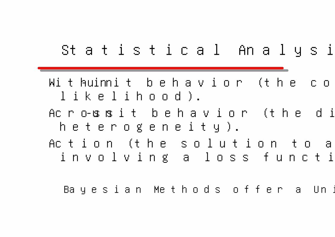
Choose the alternative with the greatest z

z is distributed according to a normal distribution

Draw from a truncated normal distribution

This is simple OLS

Conditional Distributions:

z|y,x,β

β|z,x

Model:

y|z

z|x,β

Implementation

Consumer Choice

Consumers choose offerings with attributes that provide benefits.

In most product categories there are multiple offerings, with many attributes, resulting in a complex decision process.

Consumers often use screening rules to simplify the choice process.

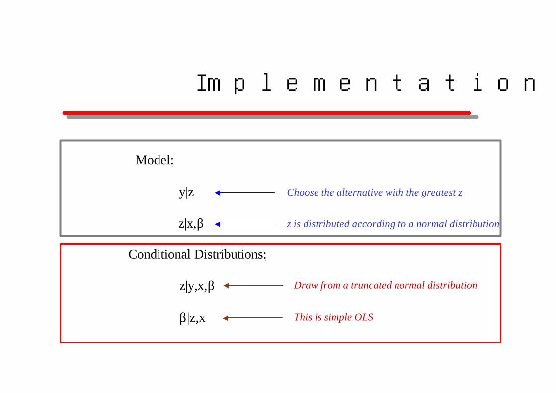
Digital Cameras

A selection of tested products (Within types, in performance order)Brand & model

Sony DSC-F707 MS 5x · · · ·Canon PowerShot G2 CF 3x · · · ·Olympus Camedia C-3040 Zoom SM 3x · · ·Olympus Camedia D-40 Zoom SM 2.8x · ·Fujifilm FinePix F601 Z SM 3x · · ·Sony Cyber-shot DSC-S75 MS 3x · · · ·HP PhotoSmart 812 SD 3x ·Kodak EasyShare DX4900 CF 2x ·Olympus Camedia E-10 CF, SM 4x · · ·Canon PowerShot S40 CF 3x · ·Casio QV-4000 CF 3x · · · ·Kyocera Finecam S4 SD 3x · · ·Panasonic Lumix DMC-LC5 SD 3x · · · ·Sony Cyber-shot DSC-P71 MS 3x · · ·Sony CD Mavica MVC-CD400 CD-R/RW 3x · · ·Minolta Dimage S404 CF 4x · ·Toshiba PDR-3310 SD 3x · · ·Kyocera Finecam S3 SD 2x · · ·

3- TO 5-MEGAPIXEL CAMERAS

Alternative Screening Rules

Conjunctive RuleAlternative must be acceptable on each of a subset of

attributes.

Disjunctive RuleAlternative must be acceptable on at least one

attribute.

Compensatory Rule“Really good” attributes can make up for “really bad”

ones.

Bayesian Decision Theory meets Behavioral Decision Theory

Will it be …..

The Thriller in ManilaAn Affair to Remember

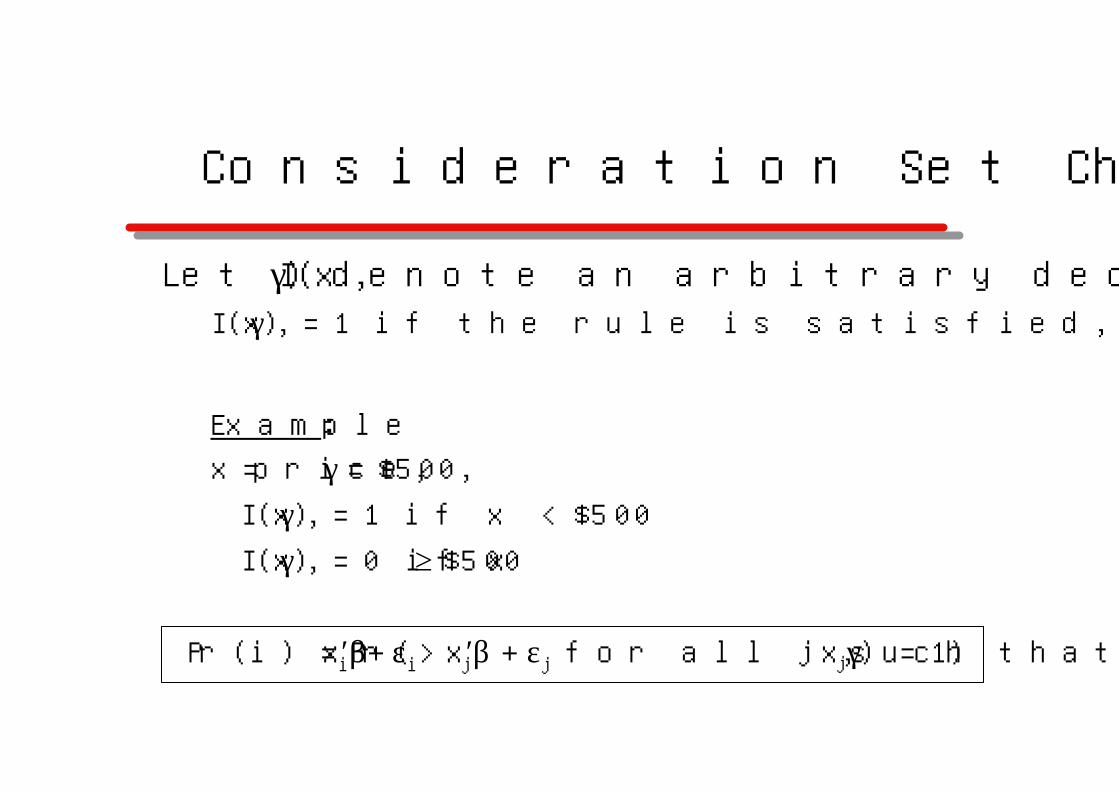
Consideration Set Choice Model

Let I(x,γ) denote an arbitrary decision rule.I(x,γ) = 1 if the rule is satisfied, =0 if not.

Example: x=price, γ = $500,

I(x,γ) = 1 if x < $500

I(x,γ) = 0 if x ≥ $500

Pr(i) = Pr(xi′β+ εi > xj′β + εj for all j such that I(xj,γ) = 1)

Conditional Distributions:z|y,x,β,I(x,γ)

γ| z, y, x

β|z,x

Choose the alternative with the greatest z, among those considered

z is distributed according to a normal distribution

Model:y|z, I(x,γ)

z|x,β

Draw from a (truncated) normal distribution

This is simple OLS

Draw from the set of allowable cut-offs

Data Augmentation and Consideration Sets

Empirical Application

Discrete choice conjoint studyAdvanced Photo System (APS)

302 participants, pre-qualified

Each participant evaluated 14 choice sets

Each set comprises 7 alternatives3 APS cameras

3 35mm cameras

None option

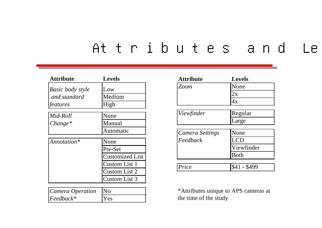
Attributes and Levels

Attribute Levels

Basic body style Low and standard Mediumfeatures High

Mid-Roll NoneChange* Manual

Automatic

Annotation* NonePre-SetCustomized ListCustom List 1Custom List 2Custom List 3

Camera Operation NoFeedback* Yes

Attribute LevelsZoom None

2x4x

Viewfinder RegularLarge

Camera Settings NoneFeedback LCD

ViewfinderBoth

Price $41 - $499

*Attributes unique to APS cameras at the time of the study

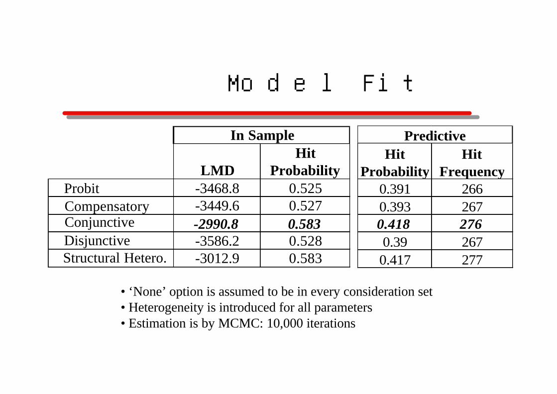
Model Fit

In Sample

LMDHit

Probability-3468.8 0.525-3449.6 0.527-2990.8 0.583-3586.2 0.528-3012.9 0.583

PredictiveHit

ProbabilityHit

Frequency0.391 2660.393 2670.418 2760.39 2670.417 277

• ‘None’ option is assumed to be in every consideration set • Heterogeneity is introduced for all parameters• Estimation is by MCMC: 10,000 iterations

ProbitCompensatoryConjunctiveDisjunctiveStructural Hetero.

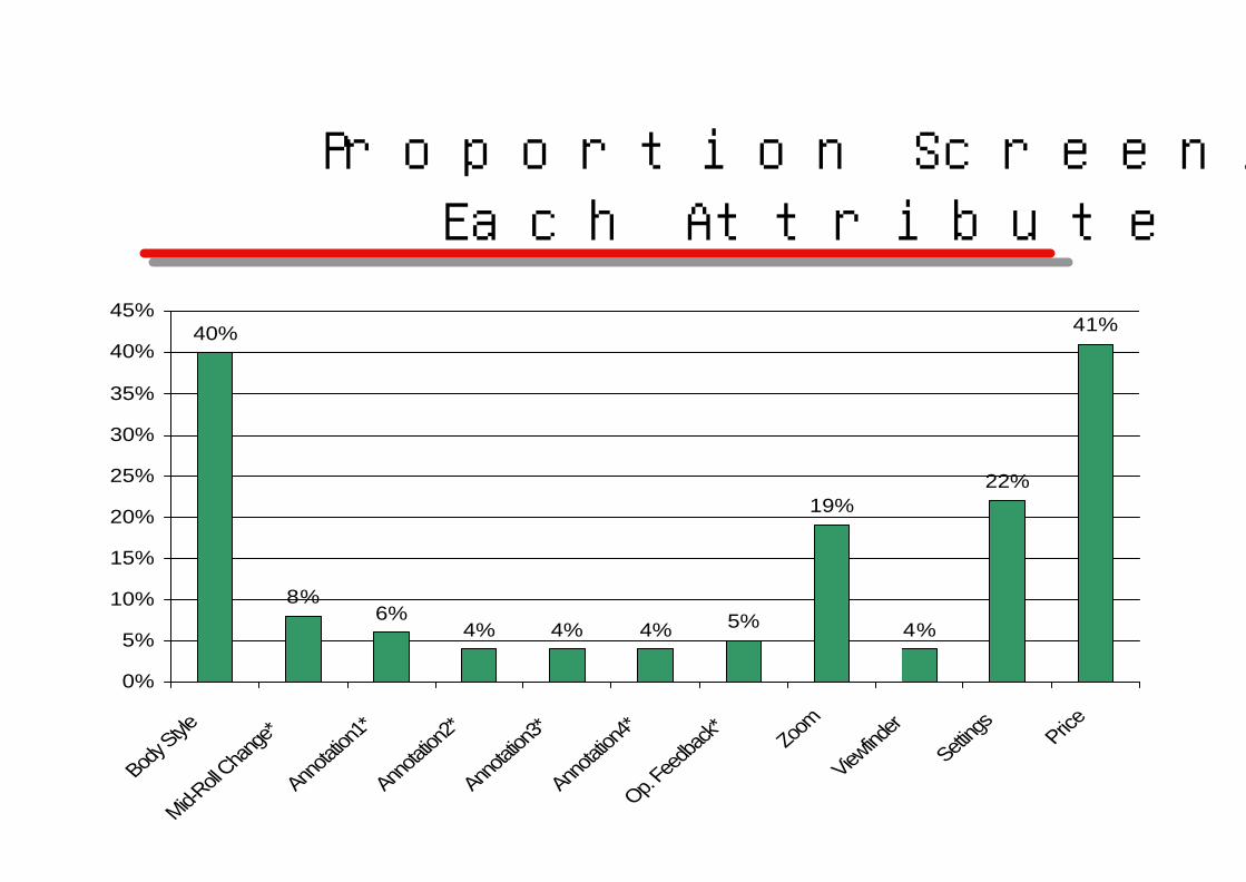
Proportion Screening on Each Attribute

40%

8%6%

4% 4% 4% 5%

19%

4%

22%

41%

0%

5%

10%

15%

20%

25%

30%

35%

40%

45%

Body S

tyle

Mid-Roll

Chang

e*

Annota

tion1*

Annota

tion2*

Annota

tion3*

Annota

tion4*

Op. Fee

dback

*Zo

om

Viewfind

er

Setting

sPrice

Distribution of Price Threshold

0%

10%

20%

30%

40%

50%

60%

70%

10%

20%

30%

41%

59%

<$276 <$356 <$425 <$499 >$499

Across Unit Analysis

The distribution of heterogeneity is typically specified as iid draws from a mixing distribution:

βi Normal(µ, Vβ)

“i” denotes the respondent/household/unit of analysis

Interdependent Preferences

Influence of the taste of othersMinivans

Abercrombie and Fitch

Extended product conceptUtility is derived from factors beyond the physical

formulation of the offering.

MechanismsSocial concerns, network externalities, signaling effects,

omitted variables (?), …

The Standard Binary Choice Model

)0Pr()Pr()1Pr( 12 >=>== iiii zUUy

iii xz εβ += '

)1,0(~ Normaliε),(~ IXNormalz β

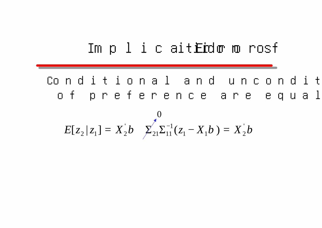
Implication of iid Errors

Conditional and unconditional expectations of preference are equal

βββ '211

11121

'212 )(]|[ XXzXzzE =−ΣΣ+= −

0

Proposed Specification

))'()(,(~

),0(~

),0(~

112

2

−− −−+

+=++=

WIWIIXNormalz

INormalu

INormaluW

Xz

ρρσβ

σ

εθρθ

θεβReflects interdependence among individuals

Exogenous Covariates

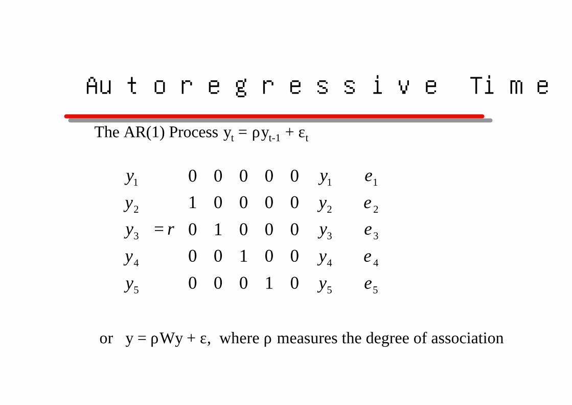
Autoregressive Time Series Models

The AR(1) Process yt = ρyt-1 + εt

+

=

5

4

3

2

1

5

4

3

2

1

5

4

3

2

1

0100000100000100000100000

εεεεε

ρ

yyyyy

yyyyy

or y = ρWy + ε, where ρ measures the degree of association

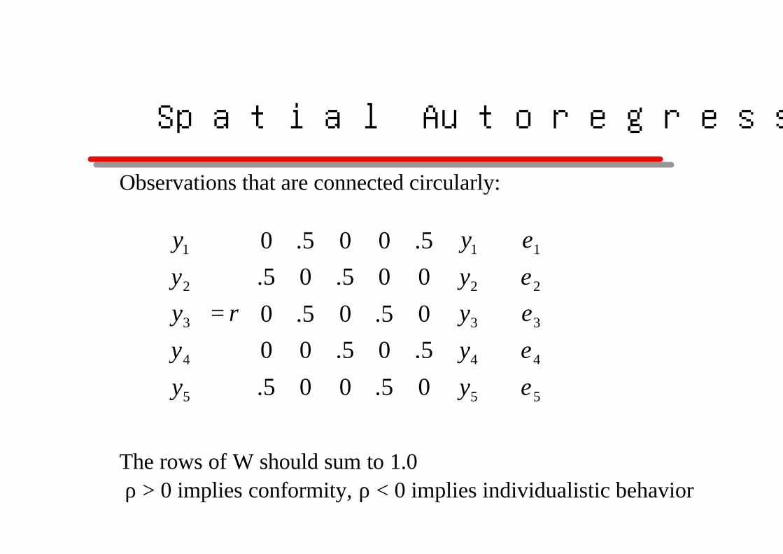
Spatial Autoregressive Models

+

=

5

4

3

2

1

5

4

3

2

1

5

4

3

2

1

05.005.5.05.0005.05.0005.05.5.005.0

εεεεε

ρ

yyyyy

yyyyy

Observations that are connected circularly:

The rows of W should sum to 1.0ρ > 0 implies conformity, ρ < 0 implies individualistic behavior

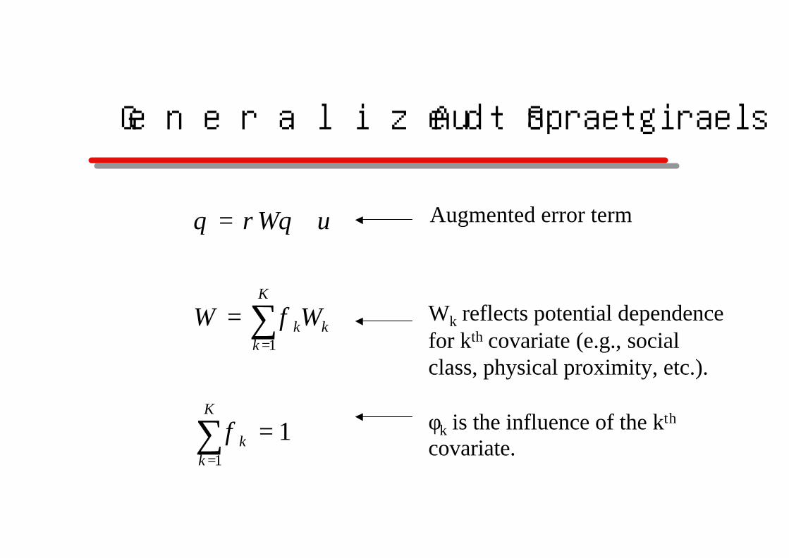
Generalized Spatial Autoregression

11

1

=

=

+=

∑

∑

=

=

K

kk

K

kkkWW

uW

φ

φ

θρθ Augmented error term

Wk reflects potential dependencefor kth covariate (e.g., socialclass, physical proximity, etc.).

φk is the influence of the kth

covariate.

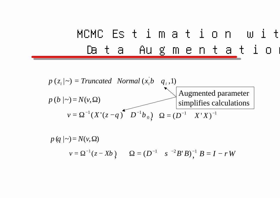
MCMC Estimation with Data Augmentation

)1,(~)|( 'iii xNormalTruncatedz θβπ +=

),(~)|( Ω= vNβπ

))('( 011 βθ −− +−Ω= DzXv 11 )'( −− +=Ω XXD

),(~)|( Ω= vNθπ

)(1 βXzv −Ω= − 121 )'( −−− +=Ω BBD σ WIB ρ−=,

,

,

Augmented parametersimplifies calculations

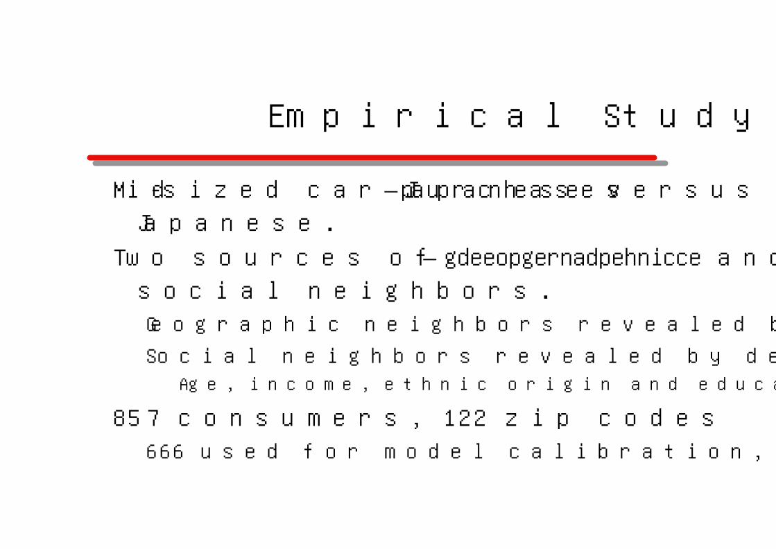
Empirical Study

Mid-sized car purchases – Japanese versus non-Japanese.

Two sources of dependence – geographic and social neighbors.Geographic neighbors revealed by zip codes.

Social neighbors revealed by demographics.Age, income, ethnic origin and education

857 consumers, 122 zip codes666 used for model calibration, 191 holdout

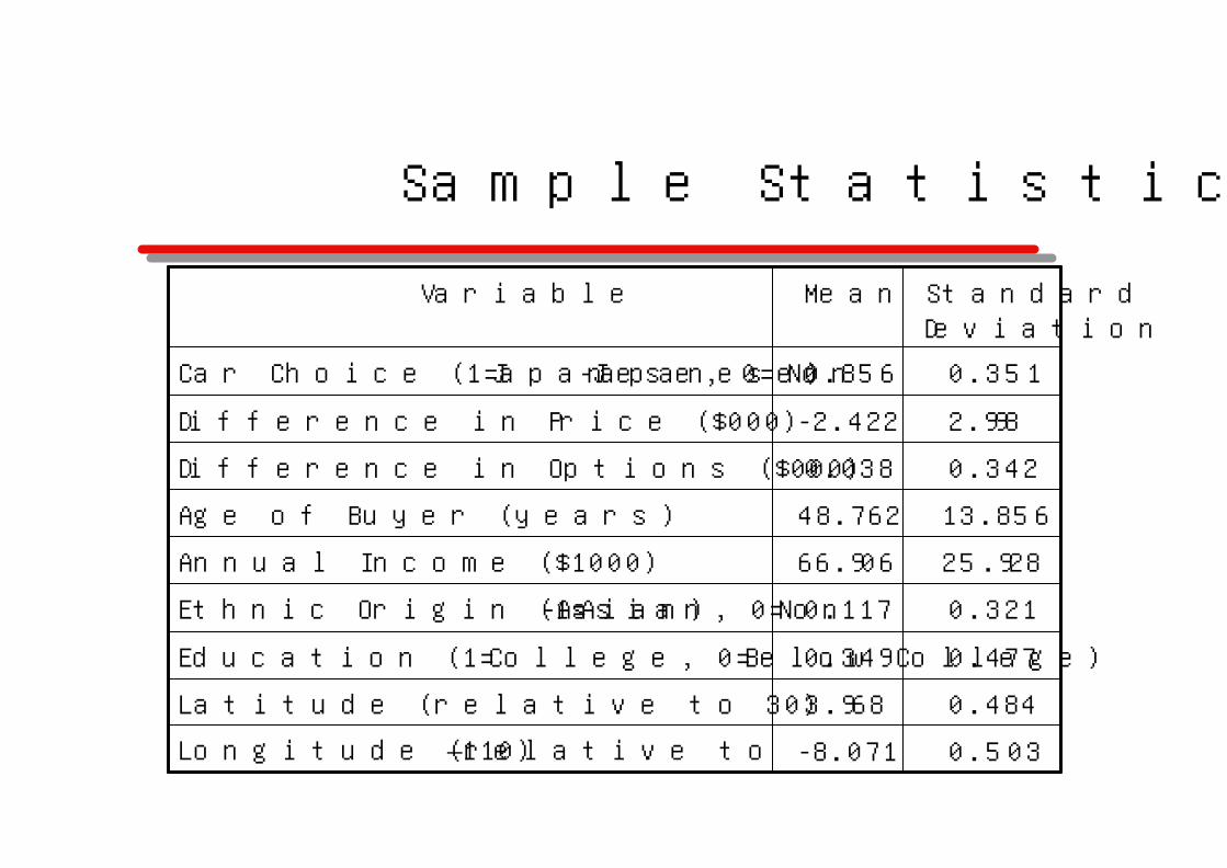
Sample Statistics

0.503-8.071Longitude (relative to –110)

0.4843.968Latitude (relative to 30)

0.4770.349Education (1=College, 0=Below College)

0.3210.117Ethnic Origin (1=Asian, 0=Non-Asian)

25.92866.906Annual Income ($1000)

13.85648.762Age of Buyer (years)

0.3420.038Difference in Options ($000)

2.998-2.422Difference in Price ($000)

0.3510.856Car Choice (1=Japanese, 0= Non-Japanese)

Standard Deviation

MeanVariable

Model Fit

0.127-133.8Mixture

0.139-151.2Demographic Neighbors

0.136-146.4Geographic Neighbors

0.158-203.8Random-Effects

0.177-237.7Probit

Predictive Fit

(MAD)

In-Sample Fit

(log marg.den)

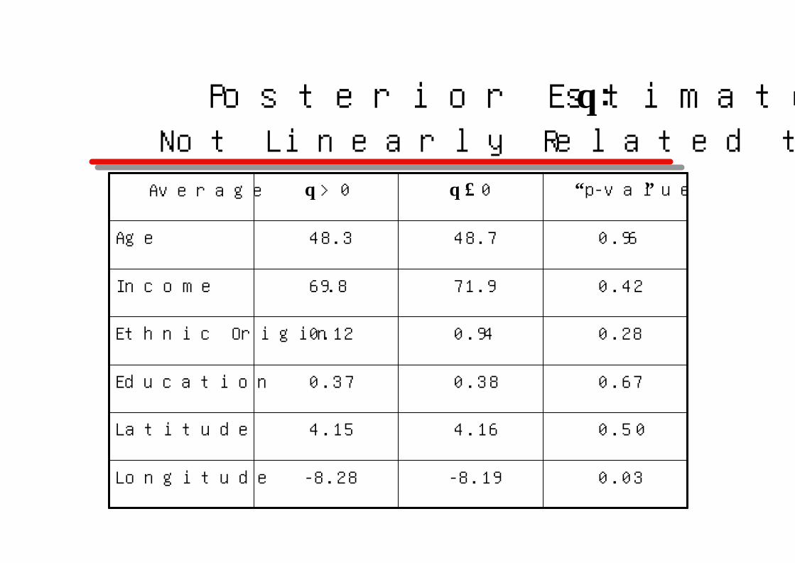
Posterior Estimates of θ:Not Linearly Related to Covariates

0.670.380.37Education

0.504.164.15Latitude

0.03-8.19-8.28Longitude

0.280.940.12Ethnic Origin

0.4271.969.8Income

0.9648.748.3Age

“p-value”θ ≤ 0θ > 0Average

Across Unit Analysis

Interdependent preferencesPervasiveNot well represented by linear model structuresNot “iid”

Extensions:Opinion leaders (extreme realizations of θ)Aspiration groups (asymmetric W)Temporal evolution (e.g., buzz)

Longitudinal and cross-sectional data

Multinomial response (multiple θ)

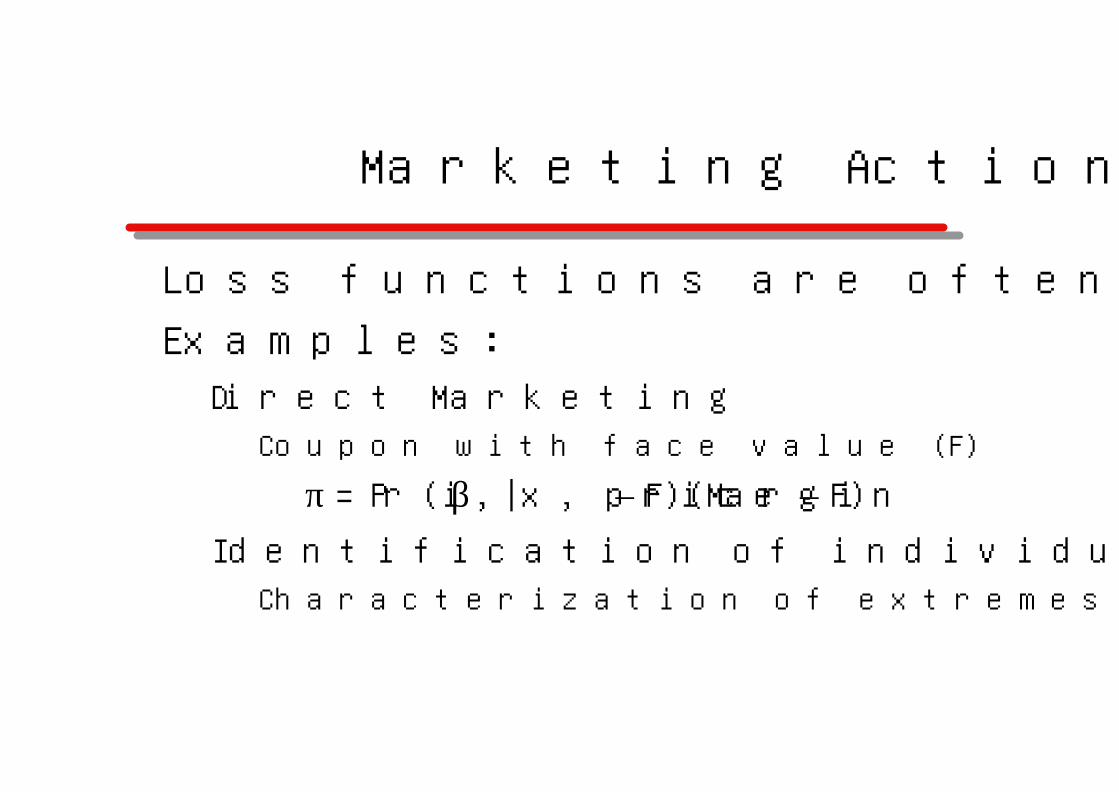
Marketing Actions

Loss functions are often easy to identify.Examples:

Direct Marketing Coupon with face value (F)

π = Pr(i ¦ β, x, price – F)(Margin – F)

Identification of individuals for further studyCharacterization of extremes

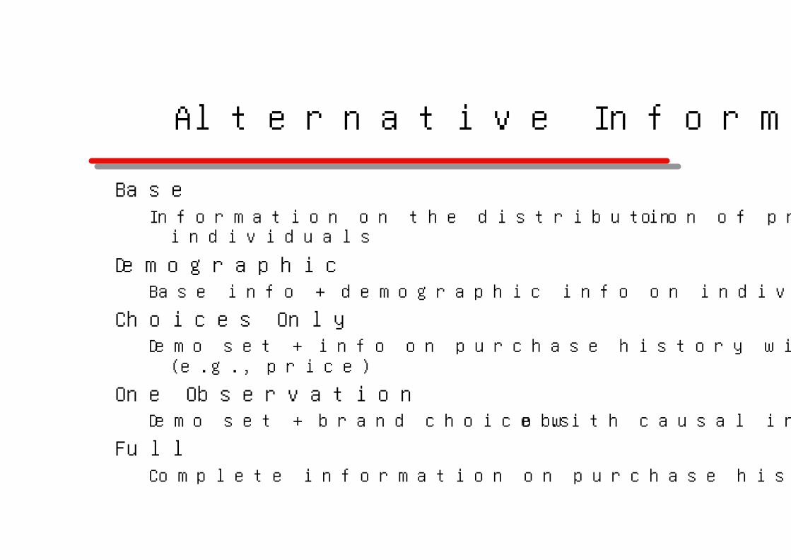
Alternative Information Sets

BaseInformation on the distribution of preferences, no specific info on

individuals

DemographicBase info + demographic info on individuals

Choices OnlyDemo set + info on purchase history without causal environment

(e.g., price)

One ObservationDemo set + brand choice with causal info for 1 obs.

FullComplete information on purchase history and causal environment

Data

Scanner panel dataset of canned tuna purchases:Brands:

Chicken of the Sea (water and oil)Starkist (water and oil)

House Brand

Data:Choices, prices, display and feature information.

Individual-level posteriors of β based on different information sets.

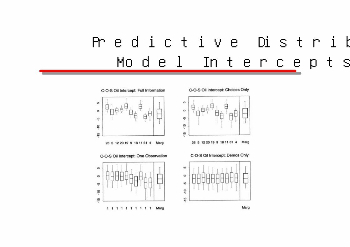
Predictive Distributions:Model Intercepts

Predictive Distributions: Price Coefficients

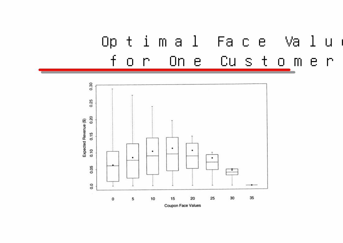
Optimal Face Values for One Customer

The Value of Information Sets

Computed via the loss function by comparing:Profits when face value is zero (F=0)Maximum profits when face value not zero (F≠0)

Relative Value

0.1380No Coupon

1.00.1459Blanket

1.120.1467Demos-Only

1.560.1500One Obs.

1.930.1529Choices-Only

2.550.1570Full

Gain Relative to Blanket Drop

Net Revenue(per purchase)

Information Set

Bayesian Statistics and Marketing

Within-unit analysisChoice and quantity, simultaneous purchase, state-

space models.

Across-unit analysisThe unit of analysis (person-activity), role of the

objective environment, relationship to motivating conditions, market segmentation.

ActionChoice simulators, product line design, exploration of

extremes, analysis of economic systems.