Greenhouse Gases - Amazon Simple Storage Service · 2014-07-10 · about greenhouse gases including...

O f f i c e o f E n v i r o n m e n t a l P o l i c y , A n a l y s i s a n d A s s e s s m e n tT E X A S N A T U R A L R E S O U R C E C O N S E R V A T I O N C O M M I S S I O N

January 2002Draft Agency Report

Greenhouse GasesA Report to the Commission

Draft

TEXAS NATURAL RESOURCE CONSERVATION COMMISSION

DECISION OF THE COMMISSIONREGARDING THE PETITIONS FOR RULEMAKING

FILED BY HENRY, LOWERRE, AND FREDERICK, LLP ON BEHALF OF PUBLICCITIZEN'S TEXAS OFFICE, CLEAN WATER ACTION, LONE STAR SIERRA CLUB,

SUSTAINABLE ENERGY AND ECONOMIC DEVELOPMENT COALITION, AND TEXAS.CAMPAIGN FOR THE ENVIRONMENT

Docket No. 2000-0845-RUL

On August 23, 2000, the Texas Natural Resource Conservation Commission (Commission)considered the petitions for rule making filed by Henry, Lowerre, and Frederick, LLP on behalf ofPublic Citizen's Texas Office, Clean Water Action, Lone Star Sierra Club, Sustainable Energy andEconomic Development Coalition, and Texas Campaign for the Environment. The first petition, filedon July 5, 2000, requests that the Commission initiate rulemaking to amend rules in 30 TAC Section101.10, General Air Quality Rules, Emissions Inventory Requirements, to expand the scope of the datacollected in the. annual air emissions inventory to include levels of carbon dioxide and methane. Thesecond petition also filed on July 5, 2000 requests the Commission create a new 30TAC Chapter 121,Control of Greenhouse Gases, that would encourage reductions in .greenhouse gases and establish anadvisory council to study the cost/benefit of reducing emissions of greenhouse gases by seven percentbelow 1990 levels.

IT IS THEREFORE THE DECISION OF THE COMMISSION pursuant to AdministrativeProcedure Act (APA), Texas Government Code, §2001.021 and Texas Water Code §5.102 to instructthe Executive Director to initiate a rulemaking proceeding and to complete the following steps byDecember 1,2001: In completing these actions, the Executive Director shall consider any EPAguidance available.

I) The Executive Director shall compile all information on quantities of greenhouse gasescurrently in the Commission's and EPA's databases. For those compound-s for which theCommission has not yet gathered information, Commission staff shall estimate those emissions;

2) The Executive Director shall survey the activities of other states and the federal governmentto assess what actions are being taken with respect to global warming, including any plansdeveloped by the states;

3) The Executive Director shall consult with other state agencies and universities regarding thescience, potential effects)and potential solutions to global warming;

4) The Executive Director shall estimate the reduction in greenhouse gases from activitiesalready completed by the Commission and actions being completed at this time both at the stateand federal levels;

5) The Executive Director shall create a registry of these emission reductions;

6) The Executive Director shall prepare a report summarizing and analyzing the findings ofitems one through four. The report should include recommendations to the Commission as toactions that the findings indicate are warranted., inc1uding any recommended changes oradditions to existing commission rules:

This Decision constitutes the decision. of the Commission required by the APA §2001.021(c).

Issued date:

i

TEXAS NATURAL RESOURCE CONSERVATION COMMISSION

A REPORT TO THE COMMISSION

Concerning Greenhouse Gases in Texas

Docket No. 2000-0845-RUL

January 2002

_________________________________Jeffrey Saitas, P.E.Executive Director

Draft Report

TABLE OF CONTENTS

Commission Decision, 2000-0845-RUL, issued Aug 25, 2000.

Overview iv

Executive Summary v

1) Summary of Greenhouse Gas Emissions inTexas.

A. Information in the TNRCC Emissions Inventory database. 1-1

B. Emissions information in the TRI database on CFC emissions. 1-2

C. Emissions information contained in other EPA and DOE databases. 1-5

D. Estimated Texas greenhouse gas emissions calculated and compiled by ICF. 1-10

2) State global warming plans.

A. Summary of state planning actions. 2-1

B. Summaries of plans developed by other states: 2-3 thru 2-33

• Alabama • Maine• California • New Jersey• Delaware • North Carolina• Hawaii • Oregon• Illinois • Tennessee• Iowa • Vermont• Kentucky • Washington• New England Governors • Wisconsin

C. EPA Guidance documents for developing Global Warming Action Plans. 2-35

3) Information from State Agencies and Universities on Global Warming.

A. Summary of recent reports.• Climate Change Science, National Research Council 3-3• Intergovernmental Panel on Climate Change Report 3-9• Royal Academy Report on Sequestration 3-23• Union of Concerned Scientists Gulf Coast Texas Report 3-25• Global Warming: A Guide to the Science 3-31

B. Bibliography of recent science reports on global warming. 3-36

ii

C. University Inputs: • Rice University 3-38• Southwest Texas State University 3-39• Texas A&M University 3-40• Texas Tech University 3-42• University of Houston 3-43• University of Texas, Austin 3-44

D. State agency contacts: • Texas Department of Aging 3-46• Texas Department of Parks and Wildlife 3-47• Texas Department of Transportation 3-48• Texas General Land Office 3-50• Texas Public Utilities Commission 3-51• Texas Water Development Board 3-52• Lower Colorado River Authority 3-52

4) Estimated greenhouse gas emission reductions

A. Estimated greenhouse gas emission reductions resulting from efficiency initiatives. 4-1

B. Estimated greenhouse gas emission reductions resulting from federal programs. 4-2

C. Estimated greenhouse gas emission reductions resulting from recent state legislation. 4-7

D. Estimated greenhouse gas emission reductions resulting from cogeneration projects 4-8 from refineries, petrochemical, and energy.

E. Other federal, state, or local programs and initiatives. 4-11

5) Consolidated registry of emission reductions in Texas. 5-1

6) Analysis and recommendations for existing commission rules. 6-1

Appendix: A. Table A1-1, Acid Rain Database. A

B. Programs for reduction in greenhouse gases. B-1

C. Methodology for estimating Texas GHG emissions. C-1

D. ICF GHG Emissions Estimates by Sector D

iii

iv

OVERVIEW

On July 5, 2000, the agency received two petitions for rulemaking from the law firm of Henry,Lowerre, and Frederick on behalf of Public Citizen’s Texas Office, Clean Water Action, LoneStar Sierra Club, Sustainable Energy and Economic Development Coalition, and TexasCampaign for the Environment. The first petition requested the agency to amend the general airrules to require the collection of carbon dioxide and methane emissions as part of the annual airemissions inventory. The second petition requested the commission to create new air rules toencourage reductions in greenhouse gases, promote the efficient use of energy, offer training inmethods to reduce carbon dioxide and methane, and develop a climate change action plan.

On August 23, 2000, the Commission responded to the petitions by issuing a commissiondecision (Docket No. 2000-0845-RUL) instructing the Executive Director to complete a numberof specific steps by December 1, 2001: • Compile information on quantities of greenhouse gases currently in the Commission’s and

EPA’s databases. Estimate emissions for which the Commission has not yet gatheredinformation.

• Survey activities of other states and the federal government with respect to global warming,including any plans developed by the states.

• Consult with other state agencies and universities about the science, potential effects andpotential solutions to global warming.

• Estimate reductions in greenhouse gases from activities already completed by theCommission and actions being completed at this time both at the state and federal levels.

• Create a registry of these emission reductions.• Prepare a report which summarizes and analyses the items above, including

recommendations for changes or additions to existing commission rules.

This report is organized in sections which correspond to each of the items in thecommission directive.

Executive Summary

This report was written in response to a decision of the Commission to compile specific information about greenhouse gases including emissions within Texas, other state plans, university research, andestimated reductions from ongoing activities. Although the report contains summary informationfrom recent scientific reports on climate change and global warming, no attempt has been made tojustify or question the conclusions of those reports. Section 1 of this report provides information on quantities of greenhouse gases currently in theCommission’s and EPA’s databases. Heretofore, the agency has not specifically requested informationon any greenhouse gases (including carbon dioxide, methane, nitrous oxide, hydrofluorocarbons,perfluorocarbons, and sulfur hexafluoride) and there is very little information about these compoundsin the annual Emissions Inventory (EI) or any other agency database. Electric utilities have reportedcarbon dioxide emissions to the EPA Acid Rain data base and the federal Toxic Release Inventory (TRI)contains information on chlorofluorocarbon (CFC) emissions since about 1990. In summary,approximately one-half of Texas greenhouse gas emissions from point sources are currently reportedto an existing database. Based on a report from the U.S. Department of Energy, the total U.S. emissionsof Carbon Dioxide, Methane, and Nitrous Oxide in 1999 amounted to about 1,795 million metric tonsof carbon equivalents (MMTCE). This total represents an average annual U.S. increase ofapproximately 1.1 percent since 1990. The TNRCC staff worked with an EPA contractor to developbaseline and trend data for Texas GHG emissions. Summary data and trend charts are contained in thissection with more detailed data in the appendix. Greenhouse gas emissions from Texas sources in 1999are estimated to be about 189 MMTCE, or approximately 10 percent of the total U.S. greenhouse gasemissions. Over the nine-year period from 1990 to 1999, Texas GHG emissions have increasedapproximately 0.7 percent per year. While estimated carbon dioxide emissions have increased,methane, nitrous oxide and CFCs (which are subject to federal regulation) have decreased in the lastdecade.

Section 2 contains summaries of 15 state Greenhouse Gas plans and reports, and a resolution from theNew England Conference of Governors. In all but one of the state greenhouse gas plans, participationin the suggested strategies is voluntary, and suggested emission reduction goals are related to those inthe Kyoto protocol. Five of the plans focus heavily on energy conservation as a way to reduce carbondioxide emissions, and many states are also relying on energy deregulation as a way to reduce emissions(burning fossil fuel to generate electricity accounts for a large percentage of carbon dioxide emissionsin many states). We are aware of two states that enacted legislation to reduce greenhouse gases.Massachusetts and Oregon passed bills that cap carbon dioxide emissions from new power plants. Bothstates allow the new facilities to pay a per-ton fee to exceed the cap.

Section 3 contains information from state agencies and universities regarding the science, potentialeffects and solutions to global warming. The first subsection provides summaries of the four latestinternational reports including a report on Climate Change in the Gulf Coast published in October 2001by the Union of Concerned Scientists. All the reports address potential temperature increases,precipitation changes and sea level increases. However, the range, timing and human contribution tothese events still contain large uncertainties. A report from the Royal Society discounts the percentageof CO2 reductions that should be attributed to land carbon sinks in the future. A bibliography of morethan 20 reports on global warming provides a reference for more detailed information about the currentscience. The staff also contacted the major Texas state universities to acquire information on the leveland extent of current university research, along with contact information for researchers and Internet

v.

links. The final subsection contains information about seven state agencies and what actions are beingpursued in response to possible global warming. The Texas Department of Aging indicated they werefocusing on the relationship between temperature increases and heat related illnesses, coupled with asubstantial growth in the older population in Texas in the coming decades. The Texas WaterDevelopment Board develops projections of water supply and demand using models which includepopulation growth and climate induced needs, but recognizes that future droughts may be more severethan have occurred historically. Section 4 contains information about estimated and potential reductions from a number of programsand projects within Texas. These include: CO2 reductions in Texas from energy efficiency initiativesfor refrigerators, freezers, and other major household appliances, GHG reductions from EPAPartnership Programs including Energy Star and the Landfill Methane Outreach Program (LMOP),GHG emission reductions from recent state legislation including HB 3415 and SB 5, and estimatedGHG reductions from cogeneration or Combined Heat and Power (CHP) projects for refineries,petrochemical, and energy. These projections include more than 21 million tons of CO2 reductions inTexas from more efficient refrigerators and freezers in the next 30 years; another 4.5 million tons ofCO2 reductions from other major appliances in the next 20 years; more then 21 million standard cubicfeet per day of methane emission reductions from landfill outreach programs in Texas; millions of cubicfeet of methane emission reductions from Texas gas companies in the Natural Gas Star Program; andover 20,000 MW of potential energy savings from cogeneration projects in Texas.

Section 5 captures some examples of greenhouse gas emission reductions in Texas. Although the staffwas aware of many energy efficiency and regulatory control projects in Texas that have or would reducegreenhouse gases, quantified reduction information was not readily available. For example, many ofthe provisions in Senate Bills 5 and 7 to reduce oxides of nitrogen in the ozone nonattainment areas ofthe state could have significant parallel reductions in carbon dioxide. However the development ofthese measures was focused on ozone reduction and made no attempt to quantify GHG emissionreductions, nor does there seem to be a direct way to relate NOx reductions to CO2 or N2O reductions.Similarly, several federal agencies collect “Top-Down” information on carbon dioxide emissions at thecorporate and national levels, with no way to tease out the Texas-only reductions. For example, theDepartment of Energy also sponsors a voluntary GHG registry program (1605b) which is based oncorporate reporting that does not lend itself to a single state analysis. This section also outlines someof the decisions that will have to be made in developing an ongoing GHG registry for Texas including:what is the baseline year, should it be voluntary, what verification is necessary, will it support a creditor banking program, electronic or hard-copy reporting, what reporting units (MMTCE or tons), etc.

Section 6 contains an analysis of existing Commission rules and whether changes or additions wouldbe required if the Commission should adopt a policy to collect data pertaining to greenhouse gases, orto regulate or control the emissions. Historically the agency has only collected emissions informationabout criteria pollutants from stationary sources. However, the general air rules were changed in 1999to include the phrase “or any other contaminant requested by the commission from individual emissionunits”. The current rules should allow the commission to collect GHG emissions information from awide variety of sources. In addition the Texas Clean Air Act clearly gives the agency broad authorityto collect information on GHG emissions even if not specifically addressed in agency rules. The natureand extent of any potential changes or additions would depend on the emission sources and the extentand type of control strategy directed by the commission.

vi.

1 - 1

Section 1. Information on quantities of greenhouse gases currently in the Commission’sand EPA’s databases.

A. Information in the TNRCC Emissions Inventory (EI) database

The Point Source Database was queried to determine current reported levels of greenhousegases. Because reporting these gases are not required by rule, it was anticipated levels would below. The reported values for 1999 are listed in the table below. These reports were captured byvoluntary reporting only and are not considered a representative sampling. Companies thatreported may have done so out of data reporting ease. Essentially, it was easier to report themthan to exclude them from their overall data reporting. The values reported were accepted on anas-reported basis and not reviewed beyond a general order of magnitude review.

Table 1.1 Greenhouse Gases Reported To TNRCC Emissions Inventory 1 For 1999

COUNTY CONTAMINANT ANNUAL (tpy) UPSET (tpy)Brazoria Carbon Dioxide 11,924.87 93,137.44

Methane 89.90 254.77

Galveston Methane 4.61 1.40

HarrisCarbon Dioxide 70.49 46.01Methane 107.98 6.28Nitrous Oxide 8.07 40.00

Harrison Methane 46.38 1.67

Hutchinson Methane 20.44 400.60

Jefferson Methane 50.79 8.37

Terry Carbon Dioxide 95.29 1,778.00Methane 0.59 0.70

Wichita Methane 1.97 0.001. Greenhouse gases are “as reported” values to the Point Source Database, (PSDB), TNRCC’sindustrial source emissions inventory database.

Additional to those emissions listed in the above table, there were 680 tons per year (tpy) offreon emitted in 1999.

1 - 2

B. Information in the Toxic Release Inventory (TRI) database on CFC emissions (directedby EPA 1990).

The Toxic Release Inventory (TRI) data base was queried for green house gases. The only datain the TRI was for chlorofluorocarbons (CFC’s), a group of compounds which EPA has beenregulating. As can be seen in the following table CFC’s have been generally decreasing, as aresult of the regulations, since 1991.

Table 1.2 TRI 2 CFC Totals by Reporting Year

Reporting Year Total Release (pounds)

1991 2,401,177

1992 2,144,650

1993 1,562,718

1994 1,662,673

1995 1,591,529

1996 1,811,032

1997 1,229,894

1998 1,106,348

1999 1,087,619 The following table summarizes the Texas data on CFC’s reported to the Toxic ReleaseInventory (http://www.epa.gov/triexplorer/). Due to the volume of their release, the top fourchemicals (Table 1.3) most significantly affect the overall downward trend. Thedichlorodifluoromethane and trichlorofluoromethane had significant decreases from 1991 to1999. The other two had an increase in the mid 1990's followed by a slight decrease in 1999(when compared to 1991).

1 - 3

Table 1.3 Total Chlorofluorocarbons Reported to TRI in 1990 - 1999Chemical Name Total Releases (lbs)DICHLORODIFLUOROMETHANE 6,237,807CHLORODIFLUOROMETHANE 3,563,936TRICHLOROFLUOROMETHANE 1,926,2471 1-DICHLORO-1-FLUOROETHANE 1,838,8972-CHLORO-1 1 1 2-TETRAFLUOROETHANE 386,149MONOCHLOROPENTAFLUOROETHANE 160,893DICHLOROTETRAFLUOROETHANE (CFC-114) 153,4332-CHLORO-1 1 1-TRIFLUOROETHANE 136,808CHLOROTETRAFLUOROETHANE 129,8001-CHLORO-1 1-DIFLUOROETHANE 56,1002 2-DICHLORO-1 1 1-TRIFLUOROETHANE 7,425BROMOCHLORODIFLUOROMETHANE 791-CHLORO-1 1 2 2-TETRAFLUOROETHANE 6

All CFC’s reported to the EPA TRI from 1991 to 1999 are listed in Table 1- 4. Note that not allchemicals have been reported each year. However, when viewed in total, the trend has beendecreasing. Table 1.4 TRI CFC Releases By Chemical For 1991 To 1999 ReportingYear Chemical Name Total Releases (lbs)1994 1 1-DICHLORO-1-FLUOROETHANE 293,3531995 1 1-DICHLORO-1-FLUOROETHANE 298,9221996 1 1-DICHLORO-1-FLUOROETHANE 384,2131997 1 1-DICHLORO-1-FLUOROETHANE 266,7671998 1 1-DICHLORO-1-FLUOROETHANE 307,0241999 1 1-DICHLORO-1-FLUOROETHANE 288,618

1994 1-CHLORO-1 1 2 2-TETRAFLUOROETHANE 31995 1-CHLORO-1 1 2 2-TETRAFLUOROETHANE 3

1995 1-CHLORO-1 1-DIFLUOROETHANE 14,0001996 1-CHLORO-1 1-DIFLUOROETHANE 16,0001997 1-CHLORO-1 1-DIFLUOROETHANE 14,0001998 1-CHLORO-1 1-DIFLUOROETHANE 6,0001999 1-CHLORO-1 1-DIFLUOROETHANE 6,100

1995 2 2-DICHLORO-1 1 1-TRIFLUOROETHANE 2,6651996 2 2-DICHLORO-1 1 1-TRIFLUOROETHANE 3,660

ReportingYear Chemical Name Total Releases (lbs)

1 - 4

1998 2 2-DICHLORO-1 1 1-TRIFLUOROETHANE 1,100

1994 2-CHLORO-1 1 1 2-TETRAFLUOROETHANE 9,0001995 2-CHLORO-1 1 1 2-TETRAFLUOROETHANE 8,9611996 2-CHLORO-1 1 1 2-TETRAFLUOROETHANE 186,2741997 2-CHLORO-1 1 1 2-TETRAFLUOROETHANE 157,5461998 2-CHLORO-1 1 1 2-TETRAFLUOROETHANE 12,1861999 2-CHLORO-1 1 1 2-TETRAFLUOROETHANE 12,182

1995 2-CHLORO-1 1 1-TRIFLUOROETHANE 2,6081998 2-CHLORO-1 1 1-TRIFLUOROETHANE 134,200

1991 BROMOCHLORODIFLUOROMETHANE 381992 BROMOCHLORODIFLUOROMETHANE 381995 BROMOCHLORODIFLUOROMETHANE 11996 BROMOCHLORODIFLUOROMETHANE 11997 BROMOCHLORODIFLUOROMETHANE 1

1994 CHLORODIFLUOROMETHANE 527,5181995 CHLORODIFLUOROMETHANE 508,3391996 CHLORODIFLUOROMETHANE 895,7111997 CHLORODIFLUOROMETHANE 640,2491998 CHLORODIFLUOROMETHANE 491,6631999 CHLORODIFLUOROMETHANE 500,456

1999 CHLOROTETRAFLUOROETHANE 129,800

1991 DICHLORODIFLUOROMETHANE 1,641,7881992 DICHLORODIFLUOROMETHANE 1,519,6691993 DICHLORODIFLUOROMETHANE 1,129,5821994 DICHLORODIFLUOROMETHANE 693,4541995 DICHLORODIFLUOROMETHANE 677,1141996 DICHLORODIFLUOROMETHANE 240,0481997 DICHLORODIFLUOROMETHANE 107,7301998 DICHLORODIFLUOROMETHANE 144,7851999 DICHLORODIFLUOROMETHANE 83,637

1991 DICHLOROTETRAFLUOROETHANE (CFC-114) 44,8751992 DICHLOROTETRAFLUOROETHANE (CFC-114) 32,1471993 DICHLOROTETRAFLUOROETHANE (CFC-114) 23,3681994 DICHLOROTETRAFLUOROETHANE (CFC-114) 8,346

ReportingYear Chemical Name Total Releases (lbs)

1 - 5

1995 DICHLOROTETRAFLUOROETHANE (CFC-114) 2,4471996 DICHLOROTETRAFLUOROETHANE (CFC-114) 5,8081997 DICHLOROTETRAFLUOROETHANE (CFC-114) 5,7431998 DICHLOROTETRAFLUOROETHANE (CFC-114) 5,8771999 DICHLOROTETRAFLUOROETHANE (CFC-114) 24,822

1991 MONOCHLOROPENTAFLUOROETHANE 39,1991992 MONOCHLOROPENTAFLUOROETHANE 27,9961993 MONOCHLOROPENTAFLUOROETHANE 33,9241994 MONOCHLOROPENTAFLUOROETHANE 5,2791995 MONOCHLOROPENTAFLUOROETHANE 5,1591996 MONOCHLOROPENTAFLUOROETHANE 441997 MONOCHLOROPENTAFLUOROETHANE 3,8581998 MONOCHLOROPENTAFLUOROETHANE 3,4441999 MONOCHLOROPENTAFLUOROETHANE 41,990

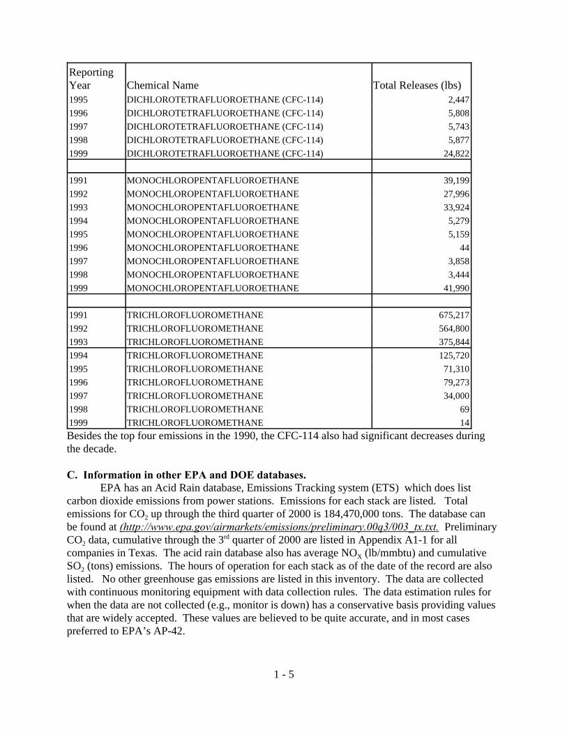
1991 TRICHLOROFLUOROMETHANE 675,2171992 TRICHLOROFLUOROMETHANE 564,8001993 TRICHLOROFLUOROMETHANE 375,8441994 TRICHLOROFLUOROMETHANE 125,7201995 TRICHLOROFLUOROMETHANE 71,3101996 TRICHLOROFLUOROMETHANE 79,2731997 TRICHLOROFLUOROMETHANE 34,0001998 TRICHLOROFLUOROMETHANE 691999 TRICHLOROFLUOROMETHANE 14Besides the top four emissions in the 1990, the CFC-114 also had significant decreases duringthe decade.

C. Information in other EPA and DOE databases.EPA has an Acid Rain database, Emissions Tracking system (ETS) which does list

carbon dioxide emissions from power stations. Emissions for each stack are listed. Totalemissions for CO2 up through the third quarter of 2000 is 184,470,000 tons. The database canbe found at (http://www.epa.gov/airmarkets/emissions/preliminary.00q3/003_tx.txt. PreliminaryCO2 data, cumulative through the 3rd quarter of 2000 are listed in Appendix A1-1 for allcompanies in Texas. The acid rain database also has average NOX (lb/mmbtu) and cumulativeSO2 (tons) emissions. The hours of operation for each stack as of the date of the record are alsolisted. No other greenhouse gas emissions are listed in this inventory. The data are collectedwith continuous monitoring equipment with data collection rules. The data estimation rules for when the data are not collected (e.g., monitor is down) has a conservative basis providing valuesthat are widely accepted. These values are believed to be quite accurate, and in most casespreferred to EPA’s AP-42.

1 - 6

D. Estimated TEXAS greenhouse gas emissions calculated and compiled by ICFConsulting. TNRCC worked with an EPA subcontractor, ICF Consulting, to develop an estimate of TexasGreenhouse gas emissions from 1990 to 1999. The inventory was developed using thefollowing objectives:• Identify the principal sources and sinks and greenhouse gases• Evaluate their relative importance• Provide the basis for assessing mitigation opportunities, and• Provide the foundation for state registries of GHG emission reductions

Several state agencies were involved with the preparation of the inventory. The TNRCCled the effort and provided most of the state data. The Texas Department of Agriculture was thesource of information on several agricultural sectors, and the Railroad Commission providedinformation on pipelines and refining systems. TNRCC coordinated data collection with the USEPA staff at the State and Local Capacity Building Branch of the Office of Air and Radiation. Additionally, staff at the United States Department of Agriculture, Forest Service were consultedregarding forestry and land use change.

Estimation StandardsThrough the work of the Intergovernmental Panel on Climate Change (IPCC), nearly 140

scientists and national experts from more than thirty countries collaborated in the creation of theRevised 1996 IPCC Guidelines for National Greenhouse Gas Inventories. 3 This guidancedocument was used to develop the inventories summarized herein. An additional guidancedocument, Good Practice Guidance and Uncertainty Management in National Greenhouse GasInventories 4, was followed to provide an inventory which is consistent with the nationalinventory. However, the default methodologies in the IPCC Guidelines and Good PracticeReport are focused upon inventories at a national scale and the data they contain are often givenas national averages and not necessarily appropriate to more regional or state-levelcircumstances. The IPCC guidelines do set a framework for defining a source and sinkcategorization system for the analysis.

EPA has revised state guidance three times since publishing the first State Workbook in1992. The workbook was revised in 1995 and 1998 to reflect changes in the IPCC methods. In1999, the workbook was thoroughly reviewed, revised and updated under the auspices of theEmissions Inventory Improvement Program. The resulting document, EIIP Volume VIII:Estimating Greenhouse Gas Emissions,5 reflects experience of state officials, a systematic ratingof uncertainty in the methods and data, and some updates to the methods. The guidanceprovides methods to estimate GHG emissions and sinks from 14 sectors:

C Combustion of fossil fuels;C Industrial processes;C Natural gas and oil systems;C Coal mining;C Municipal waste disposal;C Domesticated animals;

1 - 7

Other (5.00%)

Ag Soil Management (5.00%)Landfills (3.00%)

Enteric Fermentation (2.00%)Ozone Depleting Substances (1.00%)

Mobil Source N2O (1.00%)Coal Mining (1.00%)

Natural Gas Systems (2.00%)

Fossil Fuel Combustion (80.00%)

Exhibit 1. Greenhouse Gas Emissions

United States, 1997

C Manure management;C Flooded rice fields;C Agricultural soils;C Forest management;C Burning of agricultural crop wastes;C Municipal wastewater;C Methane and N2O emissions from mobile source combustion; and C Methane and N2O emissions from stationary source combustion.

Exhibit 1 summarizes the distribution of greenhouse gases on a national level. Based onthe experience from the states which have completed comprehensive inventories, most of theemissions and sinks are associated with a handful of sources and are similarly skewed with thenational summary (Exhibit 1).

Texas-based ApproachBased on this experience, a streamlined approach was taken for developing the Texas

inventory on key sources. This streamlined approach was also taken successfully in thedevelopment of a Florida inventory.

This framework for this streamlined approach, as applied in the Texas GHG inventory,involved four steps:• Identify “core” sources and sinks• Select additional sources• Develop inventory plan to characterize sources• Collect information and report results.

1 - 8

The six core sources for state inventories are carbon dioxide (CO2) from fossil fuel combustion,nitrous oxide (N2O) from agricultural soils, methane (CH4) from landfills, CH4 from entericfermentation, CH4 from manure management, and carbon flux from land use change andforestry. The first three are generally dominant sources in a state inventory (they comprise 81percent, 5 percent, and 3 percent of total U.S. emissions, respectively); enteric fermentation andmanure management are also significant sources (2 percent and 1 percent of emissions) and usesome of the same data as the agricultural soils analysis; and land use change and forestry is thelargest sink.

The selection of additional sources involved a screening analysis to determine whereanalysis would be most fruitful. The remaining sectors and gases (industrial processes, naturalgas systems, etc.) generally contribute far less to overall emissions and sinks, and are muchmore difficult to estimate (due to more complex methods, less available data, or both). Additional sources were selected based on the following criteria:

C Significance of the sector (in terms of likely contribution to total emissions and sinks)C Interest in the sector on the part of state staffC Availability of dataC Cost of developing an estimateC Availability of cost-effective mitigation options.

TNRCC staff determined that the following emissions sources meet one or more of thesecriteria for Texas:

C petroleum systemsC natural gas systemsC coal miningC adipic acid manufacturingC cement manufacturing.

Therefore, the inventory includes 11 sources in total, the six core sources and the five additionalsources.

After completing the screening step, the next step was to develop an InventoryPreparation Plan (IPP).6 The IPP provided details about the emissions source categories,proposed how resources would be allocated, indicated how responsibility was delegated amongstaff, outlined the documentation approach, and described a quality assurance plan.

The quality assurance plan was based primarily on a series of checks by ICF Consulting,with review by TNRCC and EPA. The plan also described the uncertainty associated with eachof the emission estimation approaches. This system provides a relative gauge of the uncertaintyassociated with each of the methods taken from the EIIP guidance.

1 - 9

The fourth and final step in the inventory process was collecting information andreporting results. A summary of the Texas GHG emissions estimates between 1990 and 1999are listed in the following charts and graphs. As shown in the pie chart (Chart 2a, following atend of Section 1), the distribution of emissions by sector is similar to the results for the nationalemissions inventory. Texas fossil fuel combustion contributes 88% of the total GHG, in carbonequivalents. This is broken into three roughly similar sized groups of industrial, electric utility,and transportation fossil fuel combustion. Detailed data from this exercise are listed in theappendix with an expanded explanation of the methodology used for each category.

A significant jump in fossil fuel combustion was noted between 1995 and 1996. Althoughseveral possible explanations were proposed to explain the anomaly, the staff was not able toconfirm a specific cause in the time available.

A detailed discussion of methodologies used to estimate emissions and additional emissionsdata for each sector in Texas are in the Appendix D.

Endnotes

1. The TNRCC Point Source Database, (PSDB). Values reported during 1999

2. EPA Toxic Release Inventory, http://www.epa.gov/triexplorer/

3. IPCC/UNEP/OECD/IEA, 1997. Revised 1996 IPCC Guidelines for National Greenhouse Gas Inventories, IPCC,United Nations Environment Programme, Organization for Economic Co-Operation and Development, InternationalEnergy Agency.

4. IPCC, 2000. Good Practice Guidance and Uncertainty Management in National Greenhouse Gas Inventories,IPCC National Greenhouse Gas Inventory Programme.

5. EIIP Volume VIII: Estimating Greenhouse Gas Emissions, available on the web athttp://www.epa.gov/ttn/chief/eiip/techreport/volume08/index.html

6. Inventory Preparation Plan for Texas Greenhouse Gas inventory, prepared for TNRCC and US EPA by ICFConsulting, 2001.

Emissions Summary

1990-1999 Emissions, by Gas (MMTCE)1990 1991 1992 1993 1994 1995 1996 1997 1998 1999

Carbon Dioxide (CO2) 155.35 152.99 155.33 155.35 155.11 154.41 166.35 167.70 170.17 169.49Fossil Fuel Combustion 149.58 147.20 149.51 152.54 152.27 151.53 163.44 164.82 167.27 166.56Land-Use Change and Forestry 4.83 4.83 4.83 1.79 1.79 1.79 1.79 1.79 1.79 1.79Cement Manufacture 0.94 0.96 0.99 1.02 1.05 1.09 1.11 1.09 1.12 1.14

Methane (CH4) 14.70 14.63 14.65 14.74 14.76 14.85 14.23 13.94 13.83 13.89Landfills 5.30 5.36 5.35 5.39 5.32 5.37 5.02 4.94 5.03 5.05Enteric Fermentation 4.52 4.55 4.68 4.80 4.91 4.99 4.90 4.72 4.70 4.73Manure Management 0.67 0.65 0.66 0.68 0.70 0.69 0.69 0.70 0.70 0.71Rice Cultivation 0.32 0.31 0.31 0.27 0.32 0.28 0.27 0.23 0.25 0.23Coal Mining 0.05 0.04 0.05 0.04 0.04 0.04 0.05 0.04 0.04 0.04Oil Systems 0.06 0.06 0.06 0.05 0.05 0.05 0.05 0.05 0.04 0.04Natural Gas Systems 3.80 3.66 3.55 3.49 3.41 3.43 3.27 3.26 3.07 3.09

Nitrous Oxide (N2O) 7.98 8.25 8.12 8.66 9.05 8.86 9.01 5.28 5.23 5.17Agricultural Soils 3.61 3.68 3.88 4.10 4.20 4.01 4.05 4.08 4.03 3.98Manure Management 0.28 0.27 0.28 0.29 0.30 0.31 0.31 0.30 0.30 0.29Adipic Acid Production 4.10 4.30 3.95 4.27 4.55 4.55 4.66 0.90 0.90 0.90

Other 28.45 28.67 28.59 26.21 26.65 26.60 26.15 22.10 21.97 21.98Total Emissions, excluding LUCF 173.21 171.04 173.26 176.96 177.13 176.33 187.80 185.13 187.45 186.75LUCF* 4.83 4.83 4.83 1.79 1.79 1.79 1.79 1.79 1.79 1.79Net Emissions 178.04 175.87 178.09 178.75 178.92 178.12 189.59 186.92 189.24 188.54

*Appears as a negative if LUCF acts as a net sink.

1990-1999 Emissions, by Gas (MMT of Gas)1990 1991 1992 1993 1994 1995 1996 1997 1998 1999

Carbon Dioxide (CO2) 569.61 560.98 569.53 569.61 568.73 566.16 609.94 614.89 623.97 621.47Fossil Fuel Combustion 548.47 539.74 548.19 559.31 558.32 555.60 599.30 604.33 613.31 610.73Land-Use Change and Forestry 17.71 17.71 17.71 6.56 6.56 6.56 6.56 6.56 6.56 6.56Cement Manufacture 3.44 3.53 3.64 3.74 3.85 3.99 4.08 4.00 4.10 4.17

Methane (CH4) 2.57 2.55 2.56 2.57 2.58 2.59 2.49 2.43 2.42 2.42Landfills 0.93 0.94 0.93 0.94 0.93 0.94 0.88 0.86 0.88 0.88Enteric Fermentation 0.79 0.79 0.82 0.84 0.86 0.87 0.86 0.82 0.82 0.83Manure Management 0.12 0.11 0.11 0.12 0.12 0.12 0.12 0.12 0.12 0.12Rice Cultivation 0.06 0.05 0.05 0.05 0.06 0.05 0.05 0.04 0.04 0.04Coal Mining 0.01 0.01 0.01 0.01 0.01 0.01 0.01 0.01 0.01 0.01Oil Systems 0.01 0.01 0.01 0.01 0.01 0.01 0.01 0.01 0.01 0.01Natural Gas Systems 0.66 0.64 0.62 0.61 0.60 0.60 0.57 0.57 0.54 0.54

Nitrous Oxide (N2O) 0.09 0.10 0.10 0.10 0.11 0.10 0.11 0.06 0.06 0.06Agricultural Soils 0.04 0.04 0.05 0.05 0.05 0.05 0.05 0.05 0.05 0.05Manure Management 0.00 0.00 0.00 0.00 0.00 0.00 0.00 0.00 0.00 0.00Adipic Acid Production 0.05 0.05 0.05 0.05 0.05 0.05 0.06 0.01 0.01 0.01

1990-1999 Emissions, Percentage of Net GHG Emissions (Percentages calculated on MMTCE basis)1990 1991 1992 1993 1994 1995 1996 1997 1998 1999

Carbon Dioxide (CO2) 87.3% 87.0% 87.2% 86.9% 86.7% 86.7% 87.7% 89.7% 89.9% 89.9%Fossil Fuel Combustion 84.0% 83.7% 83.9% 85.3% 85.1% 85.1% 86.2% 88.2% 88.4% 88.3%Land-Use Change and Forestry 2.7% 2.7% 2.7% 1.0% 1.0% 1.0% 0.9% 1.0% 0.9% 0.9%Cement Manufacture 0.5% 0.5% 0.6% 0.6% 0.6% 0.6% 0.6% 0.6% 0.6% 0.6%

Methane (CH4) 8.3% 8.3% 8.2% 8.2% 8.2% 8.3% 7.5% 7.5% 7.3% 7.4%Landfills 3.0% 3.0% 3.0% 3.0% 3.0% 3.0% 2.6% 2.6% 2.7% 2.7%Enteric Fermentation 2.5% 2.6% 2.6% 2.7% 2.7% 2.8% 2.6% 2.5% 2.5% 2.5%Manure Management 0.4% 0.4% 0.4% 0.4% 0.4% 0.4% 0.4% 0.4% 0.4% 0.4%Rice Cultivation 0.2% 0.2% 0.2% 0.1% 0.2% 0.2% 0.1% 0.1% 0.1% 0.1%Coal Mining 0.0% 0.0% 0.0% 0.0% 0.0% 0.0% 0.0% 0.0% 0.0% 0.0%Oil Systems 0.0% 0.0% 0.0% 0.0% 0.0% 0.0% 0.0% 0.0% 0.0% 0.0%Natural Gas Systems 2.1% 2.1% 2.0% 2.0% 1.9% 1.9% 1.7% 1.7% 1.6% 1.6%

Nitrous Oxide (N2O) 4.5% 4.7% 4.6% 4.8% 5.1% 5.0% 4.8% 2.8% 2.8% 2.7%Agricultural Soils 2.0% 2.1% 2.2% 2.3% 2.3% 2.2% 2.1% 2.2% 2.1% 2.1%Manure Management 0.2% 0.2% 0.2% 0.2% 0.2% 0.2% 0.2% 0.2% 0.2% 0.2%Adipic Acid Production 2.3% 2.4% 2.2% 2.4% 2.5% 2.6% 2.5% 0.5% 0.5% 0.5%

1990-1999 Emissions, Percentage of Gas Emissions (Percentages calculated on MMT basis for each gas)1990 1991 1992 1993 1994 1995 1996 1997 1998 1999

Carbon Dioxide (CO2) 100.0% 100.0% 100.0% 100.0% 100.0% 100.0% 100.0% 100.0% 100.0% 100.0%Fossil Fuel Combustion 96.3% 96.2% 96.3% 98.2% 98.2% 98.1% 98.3% 98.3% 98.3% 98.3%Land-Use Change and Forestry 3.1% 3.2% 3.1% 1.2% 1.2% 1.2% 1.1% 1.1% 1.1% 1.1%Cement Manufacture 0.6% 0.6% 0.6% 0.7% 0.7% 0.7% 0.7% 0.7% 0.7% 0.7%

Methane (CH4) 100.0% 100.0% 100.0% 100.0% 100.0% 100.0% 100.0% 100.0% 100.0% 100.0%Landfills 36.1% 36.6% 36.5% 36.6% 36.0% 36.1% 35.3% 35.4% 36.4% 36.4%Enteric Fermentation 30.7% 31.1% 31.9% 32.6% 33.3% 33.6% 34.4% 33.8% 34.0% 34.0%Manure Management 4.5% 4.4% 4.5% 4.6% 4.8% 4.7% 4.8% 5.0% 5.0% 5.1%Rice Cultivation 2.1% 2.1% 2.1% 1.8% 2.1% 1.9% 1.9% 1.7% 1.8% 1.7%Coal Mining 0.3% 0.3% 0.3% 0.3% 0.3% 0.3% 0.3% 0.3% 0.3% 0.3%Oil Systems 0.4% 0.4% 0.4% 0.4% 0.4% 0.3% 0.3% 0.3% 0.3% 0.3%Natural Gas Systems 25.8% 25.0% 24.2% 23.7% 23.1% 23.1% 22.9% 23.4% 22.2% 22.2%

Nitrous Oxide (N2O) 100.0% 100.0% 100.0% 100.0% 100.0% 100.0% 100.0% 100.0% 100.0% 100.0%Agricultural Soils 45.2% 44.6% 47.8% 47.3% 46.4% 45.2% 44.9% 77.3% 77.1% 77.0%Manure Management 3.5% 3.3% 3.5% 3.4% 3.3% 3.5% 3.4% 5.7% 5.7% 5.7%Adipic Acid Production 51.4% 52.1% 48.7% 49.3% 50.2% 51.4% 51.7% 17.0% 17.1% 17.4%

Emissions by Gas, 1990-1999 (MMTCE)1990 1991 1992 1993 1994 1995 1996 1997 1998 1999

Carbon Dioxide 155.35 152.99 155.33 155.35 155.11 154.41 166.35 167.70 170.17 169.49Methane 14.70 14.63 14.65 14.74 14.76 14.85 14.23 13.94 13.83 13.89Nitrous Oxide 7.98 8.25 8.12 8.66 9.05 8.86 9.01 5.28 5.23 5.17TOTAL 178.04 175.87 178.09 178.75 178.92 178.12 189.59 186.92 189.24 188.54

1991-1999 Percentage Emissions Changes (Percentages calculated on MMTCE basis)1991 1992 1993 1994 1995 1996 1997 1998 1999 1990-1999

Carbon Dioxide (CO2) -1.5% 1.5% 0.0% -0.2% -0.5% 7.7% 0.8% 1.5% -0.4% 9.1%

Fossil Fuel Combustion -1.6% 1.6% 2.0% -0.2% -0.5% 7.9% 0.8% 1.5% -0.4% 11.4%Land-Use Change and Forestry 0.0% 0.0% -62.9% 0.0% 0.0% 0.0% 0.0% 0.0% 0.0% -62.9%Cement Manufacture 2.8% 2.9% 2.9% 2.9% 3.6% 2.3% -2.0% 2.4% 1.9% 21.4%

Methane (CH4) -0.5% 0.1% 0.6% 0.1% 0.6% -4.2% -2.1% -0.8% 0.4% -5.5%

LandfillsEnteric Fermentation 0.7% 2.8% 2.7% 2.3% 1.4% -1.7% -3.8% -0.3% 0.6% 4.7%Manure Management -2.7% 0.9% 3.9% 3.0% -1.0% -0.9% 1.1% 0.0% 1.5% 5.7%Rice Cultivation -2.8% 2.3% -15.1% 18.8% -10.2% -6.3% -13.1% 9.3% -8.5% -26.6%Coal Mining -3.5% 2.3% -0.9% -4.1% 0.6% 4.7% -3.3% -1.4% 0.9% -4.8%Oil SystemsNatural Gas Systems

Nitrous Oxide (N2O) 3.3% -1.6% 6.7% 4.5% -2.1% 1.7% -41.4% -1.0% -1.2% -35.3%

Agricultural Soils 2.0% 5.6% 5.6% 2.6% -4.7% 1.1% 0.9% -1.2% -1.4% 10.2%Manure Management -2.5% 4.9% 3.6% 2.8% 1.6% -0.6% -1.5% -0.3% -2.0% 5.9%Adipic Acid Production 4.9% -8.2% 8.1% 6.5% 0.1% 2.3% -80.8% 0.0% 0.0% -78.1%

Chart 1B. Profile of Texas GHG Emissions by Gas, 1999

Nitrous Oxide2.7%

Carbon Dioxide89.9%

Methane7.4%

Chart 1A. Profile of Texas GHG Emissions by Gas, 1990

Nitrous Oxide4.5%

Carbon Dioxide87.3%

Methane8.3%

Chart 2. Summary of Texas GHG Emissions, 1990-1999 (MMTCE)

0

20

40

60

80

100

120

140

160

180

200

1990 1991 1992 1993 1994 1995 1996 1997 1998 1999Year

Em

iss

ion

s (

MM

TC

E)

Landfills

Oil, Gas, and Coal

LUCF

Industrial

Agriculture

Commercial Fossil FuelCombustion

Residential Fossil FuelCombustion

Transportation Fossil FuelCombustion

Electric Utility Fossil FuelCombustion

Industrial Fossil FuelCombustion

Chart 2A. 1999 GHG Emissions in Texas by Sector

Landfills2.7%

Industrial Fossil Fuel Combustion

29.6%

Industrial 1.1%

LUCF0.9%

Commercial & Residential Fossil Fuel Combustion

3.3%

Agriculture5.3%

Transportation Fossil Fuel Combustion

26.2%

Electric Utility Fossil Fuel

Combustion29.3%

Oil, Gas & Coal1.7%

GWPsMethane (CH4) 21Nitrous Oxide (N2O) 310

Carbon Dioxide (CO2) 1Emissions (MMTCE)Sectors 1990 1991 1992 1993 1994 1995 1996 1997 1998 1999Fossil Fuel Combustion 149.58 147.20 149.51 152.54 152.27 151.53 163.44 164.82 167.27 166.56LUCF 4.83 4.83 4.83 1.79 1.79 1.79 1.79 1.79 1.79 1.79Agriculture 9.38 9.45 9.81 10.14 10.44 10.28 10.21 10.03 9.98 9.93Industrial 5.04 5.27 4.94 5.29 5.60 5.64 5.77 1.99 2.01 2.03Oil, Gas, and Coal 3.90 3.76 3.65 3.59 3.51 3.52 3.36 3.36 3.15 3.17Landfills 5.30 5.36 5.35 5.39 5.32 5.37 5.02 4.94 5.03 5.05

Chart 3. Texas GHG Emissions, 1990-1999

0

50

100

150

200

1990 1991 1992 1993 1994 1995 1996 1997 1998 1999Year

Em

issi

on

s (M

MT

CE

)

Fossil Fuel Combustion CO2 All Other Sources

Chart 4. Texas Methane (CH4) Emissions, 1990-1999

02468

10121416

1990 1991 1992 1993 1994 1995 1996 1997 1998 1999

Year

Em

issi

on

s (M

MT

CE

)

Total Methane Emissions Landfills Enteric FermentationManure Management Rice Cultivation Coal MiningOil Systems Natural Gas Systems

Chart 5. Texas Nitrous Oxide (N2O) Emissions, 1990-1999

0

2

4

6

8

10

1990 1991 1992 1993 1994 1995 1996 1997 1998 1999

Year

Em

mis

ion

s (M

MT

CE

)

Total Nitrous Oxide Emissions Agricultural SoilsManure Management Adipic Acid Production

Notes:

Sectors have been combined in order to limit the number of lines/shaded areasAgriculture includes enteric fermentation, manure management, ag soils, and rice cultivation. Industrial includes Adipic Acid Production and Cement Manfacture. Oil, Gas, and Coal refer to Oil and Gas Systems and Coal Mining, not oil, gas, and coal consumption.

Chart 6. Summary of Texas GHG Emissions, 1990-1999 (MMTCE)

0

10

20

30

40

50

60

70

1990 1991 1992 1993 1994 1995 1996 1997 1998 1999Year

Em

issi

on

s (M

MT

CE

)

Industrial Fossil FuelCombustion

Electric Utility Fossil FuelCombustion

Transportation Fossil FuelCombustion

Agriculture

Residential + CommercialFossil Fuel Combustion

Industrial

LUCF

Landfills

Oil, Gas, and Coal

Chart 8. Texas GHG Emissions by Sector, 1990-1999(excluding Fossil Fuel Combustion)

0

2

4

6

8

10

12

1990 1991 1992 1993 1994 1995 1996 1997 1998 1999Year

Em

issi

on

s (M

MT

CE

)

Agriculture

Industrial

LUCF

Oil, Gas, and Coal

Landfills

Chart 7. Texas GHG Emissions by Sector, 1990-1999(excluding Fossil Fuel Combustion)

0

5

10

15

20

25

30

35

1990 1991 1992 1993 1994 1995 1996 1997 1998 1999Year

Em

issi

on

s (M

MT

CE

)

Landfills

Oil, Gas, and Coal

LUCF

Industrial

Agriculture

Fossil Fuel Combustion Emissions'[Texas Energy.xls]Emissions

Emissions by Consumption Sector, 1990-1999 (MMTCE)1990 1991 1992 1993 1994 1995 1996 1997 1998 1999

Residential 3.54 3.58 3.46 3.66 3.43 3.30 3.57 3.70 3.30 3.19Coal 0.00 0.00 0.00 0.00 0.00 0.00 0.00 0.00 0.00 0.00Petroleum 0.38 0.25 0.21 0.23 0.23 0.21 0.15 0.22 0.28 0.56Natural Gas 3.16 3.33 3.24 3.43 3.20 3.10 3.42 3.48 3.01 2.63

Commercial 3.28 3.29 3.34 2.94 3.05 3.46 2.98 3.46 2.88 3.01Coal 0.00 0.00 0.00 0.00 0.00 0.00 0.00 0.00 0.01 0.00Petroleum 0.69 0.58 0.55 0.33 0.35 0.31 0.32 0.26 0.31 0.44Natural Gas 2.59 2.71 2.79 2.61 2.71 3.15 2.66 3.21 2.56 2.56

Industrial 52.34 50.96 52.91 52.89 53.37 53.74 59.77 58.65 57.74 55.81Coal 1.60 1.64 1.57 1.84 2.15 1.66 1.91 1.92 1.74 1.73Petroleum 20.21 19.32 21.50 19.67 20.35 19.25 22.12 22.83 21.60 21.83Natural Gas 30.53 30.01 29.84 31.39 30.87 32.83 35.73 33.90 34.41 32.25

Transportation 42.12 41.30 42.49 42.08 42.96 41.72 45.15 46.02 48.59 49.33Coal 0.00 0.00 0.00 0.00 0.00 0.00 0.00 0.00 0.00 0.00Petroleum 40.53 40.08 41.26 40.86 41.53 40.49 44.03 44.80 47.59 48.28Natural Gas 1.59 1.23 1.22 1.22 1.44 1.23 1.13 1.22 0.99 1.05

Electric Utilities 48.30 48.06 47.31 50.96 49.45 49.30 51.97 52.98 54.76 55.22Coal 33.17 33.10 32.95 35.00 33.93 33.83 36.55 37.38 36.41 37.44Petroleum 0.11 0.05 0.06 0.12 0.07 0.05 0.12 0.04 0.03 0.03Natural Gas 15.01 14.90 14.30 15.84 15.45 15.42 15.31 15.56 18.32 17.75

TOTAL 149.58 147.20 149.51 152.54 152.27 151.53 163.44 164.82 167.27 166.56

Res+Comm 6.82 6.87 6.81 6.60 6.49 6.76 6.55 7.17 6.18 6.20

Chart 9. Fossil Fuel Combustion Emissions by Sector, 1990-1999

0

10

20

30

40

50

60

70

1 2 3 4 5 6 7 8 9 10

Year

Em

issi

on

s (M

MT

CE

)

Industrial

Electric Utilities

Transportation

Residential

Commercial

Emissions by Consumption Sector, 1990-1999 (MMT CO2)1990 1991 1992 1993 1994 1995 1996 1997 1998 1999

Residential 12.99 13.13 12.69 13.43 12.58 12.12 13.08 13.58 12.09 11.70Coal 0.01 0.01 0.01 0.00 0.00 0.00 0.00 0.00 0.01 0.01Petroleum 1.40 0.92 0.79 0.84 0.83 0.76 0.54 0.81 1.04 2.06Natural Gas 11.59 12.20 11.89 12.59 11.75 11.36 12.55 12.78 11.04 9.63

Commercial 12.02 12.07 12.26 10.77 11.20 12.67 10.93 12.70 10.56 11.04Coal 0.02 0.02 0.01 0.01 0.00 0.00 0.00 0.00 0.02 0.01Petroleum 2.52 2.12 2.02 1.20 1.28 1.14 1.16 0.94 1.15 1.63Natural Gas 9.48 9.93 10.23 9.56 9.92 11.53 9.77 11.76 9.39 9.40

Industrial 191.92 186.86 194.00 193.95 195.69 197.05 219.14 215.06 211.73 204.62Coal 5.87 6.02 5.76 6.75 7.89 6.08 7.02 7.05 6.39 6.35Petroleum 74.11 70.82 78.82 72.11 74.61 70.59 81.09 83.70 79.18 80.04Natural Gas 111.95 110.02 109.42 115.09 113.19 120.38 131.03 124.31 126.15 118.23

Transportation 154.45 151.45 155.78 154.29 157.53 152.99 165.57 168.73 178.16 180.89Coal 0.00 0.00 0.00 0.00 0.00 0.00 0.00 0.00 0.00 0.00Petroleum 148.62 146.95 151.30 149.82 152.26 148.48 161.43 164.27 174.51 177.04Natural Gas 5.83 4.50 4.48 4.47 5.27 4.51 4.14 4.47 3.64 3.85

Electric Utilities 177.09 176.23 173.45 186.87 181.32 180.77 190.57 194.25 200.77 202.48Coal 121.63 121.38 120.80 128.33 124.40 124.04 134.00 137.05 133.49 137.29Petroleum 0.42 0.20 0.21 0.46 0.26 0.17 0.45 0.15 0.12 0.12Natural Gas 55.04 54.65 52.44 58.09 56.66 56.56 56.12 57.06 67.17 65.07

TOTAL 548.47 539.74 548.19 559.31 558.32 555.60 599.30 604.33 613.31 610.73

Emissions by Fuel, 1990-1999 (MMTCE)1990 1991 1992 1993 1994 1995 1996 1997 1998 1999

Coal 34.78 34.75 34.52 36.84 36.08 35.49 38.46 39.30 38.16 39.18Residential 0.00 0.00 0.00 0.00 0.00 0.00 0.00 0.00 0.00 0.00Commercial 0.00 0.00 0.00 0.00 0.00 0.00 0.00 0.00 0.01 0.00Industrial 1.60 1.64 1.57 1.84 2.15 1.66 1.91 1.92 1.74 1.73Transportation 0.00 0.00 0.00 0.00 0.00 0.00 0.00 0.00 0.00 0.00Electric Utilities 33.17 33.10 32.95 35.00 33.93 33.83 36.55 37.38 36.41 37.44

Petroleum 61.93 60.28 63.58 61.21 62.52 60.31 66.73 68.15 69.82 71.15Residential 0.38 0.25 0.21 0.23 0.23 0.21 0.15 0.22 0.28 0.56Commercial 0.69 0.58 0.55 0.33 0.35 0.31 0.32 0.26 0.31 0.44Industrial 20.21 19.32 21.50 19.67 20.35 19.25 22.12 22.83 21.60 21.83Transportation 40.53 40.08 41.26 40.86 41.53 40.49 44.03 44.80 47.59 48.28Electric Utilities 0.11 0.05 0.06 0.12 0.07 0.05 0.12 0.04 0.03 0.03

Natural Gas 52.88 52.17 51.40 54.49 53.67 55.73 58.26 57.37 59.29 56.23Residential 3.16 3.33 3.24 3.43 3.20 3.10 3.42 3.48 3.01 2.63Commercial 2.59 2.71 2.79 2.61 2.71 3.15 2.66 3.21 2.56 2.56Industrial 30.53 30.01 29.84 31.39 30.87 32.83 35.73 33.90 34.41 32.25Transportation 1.59 1.23 1.22 1.22 1.44 1.23 1.13 1.22 0.99 1.05Electric Utilities 15.01 14.90 14.30 15.84 15.45 15.42 15.31 15.56 18.32 17.75

TOTAL 149.58 147.20 149.51 152.54 152.27 151.53 163.44 164.82 167.27 166.56

Chart 10. Fossil Fuel Combustion Emissions by Fuel, 1990-1999

0

20

40

60

80

1990

1991

1992

1993

1994

1995

1996

1997

1998

1999

Year

Em

issi

on

s (M

MT

CE

)

PetroleumNatural GasCoal

Emissions by Fuel, 1990-1999 (MMT CO2)1990 1991 1992 1993 1994 1995 1996 1997 1998 1999

Coal 127.52 127.42 126.59 135.09 132.29 130.12 141.02 144.09 139.91 143.65Residential 0.01 0.01 0.01 0.00 0.00 0.00 0.00 0.00 0.01 0.01Commercial 0.02 0.02 0.01 0.01 0.00 0.00 0.00 0.00 0.02 0.01Industrial 5.87 6.02 5.76 6.75 7.89 6.08 7.02 7.05 6.39 6.35Transportation 0.00 0.00 0.00 0.00 0.00 0.00 0.00 0.00 0.00 0.00Electric Utilities 121.63 121.38 120.80 128.33 124.40 124.04 134.00 137.05 133.49 137.29

Petroleum 227.06 221.01 233.13 224.43 229.25 221.15 244.67 249.87 256.00 260.89Residential 1.40 0.92 0.79 0.84 0.83 0.76 0.54 0.81 1.04 2.06Commercial 2.52 2.12 2.02 1.20 1.28 1.14 1.16 0.94 1.15 1.63Industrial 74.11 70.82 78.82 72.11 74.61 70.59 81.09 83.70 79.18 80.04Transportation 148.62 146.95 151.30 149.82 152.26 148.48 161.43 164.27 174.51 177.04Electric Utilities 0.42 0.20 0.21 0.46 0.26 0.17 0.45 0.15 0.12 0.12

Natural Gas 193.89 191.30 188.47 199.79 196.79 204.34 213.60 210.37 217.40 206.19Residential 11.59 12.20 11.89 12.59 11.75 11.36 12.55 12.78 11.04 9.63Commercial 9.48 9.93 10.23 9.56 9.92 11.53 9.77 11.76 9.39 9.40Industrial 111.95 110.02 109.42 115.09 113.19 120.38 131.03 124.31 126.15 118.23Transportation 5.83 4.50 4.48 4.47 5.27 4.51 4.14 4.47 3.64 3.85Electric Utilities 55.04 54.65 52.44 58.09 56.66 56.56 56.12 57.06 67.17 65.07

TOTAL 548.47 539.74 548.19 559.31 558.32 555.60 599.30 604.33 613.31 610.73

Emissions from Landfills

Landfill Methane Emissions 1990-19991990 1991 1992 1993 1994 1995 1996 1997 1998 1999

30 year WIP (MMT MSW) 349 358 368 378 389 399 411 422 434 448In Large LFs 316 324 333 342 351 361 371 381 392 405In Small LFs 33 34 35 36 37 38 39 40 42 43

Net Methane Emissions (MMT) 0.93 0.94 0.93 0.94 0.93 0.94 0.88 0.86 0.88 0.88Net Methane Emissions (MMTCE) 5.30 5.36 5.35 5.39 5.32 5.37 5.02 4.94 5.03 5.05

Chart 11. Methane Emissions from Landfills, 1990-1999

0

100

200

300

400

500

1990199119921993199419951996199719981999

Year

Was

te In

Pla

ce (

met

ric

ton

s)

0.00

1.00

2.00

3.00

4.00

5.00

6.00

Em

issi

on

s (M

MT

CE

)

30 year WasteIn Place

MethaneEmissions

Agricultural Sources

Enteric Fermentation, 1990-1999 (MMTCE)1990 1991 1992 1993 1994 1995 1996 1997 1998 1999

Dairy 0.32 0.30 0.30 0.32 0.34 0.34 0.32 0.31 0.30 0.28Beef 3.98 4.03 4.16 4.27 4.38 4.46 4.40 4.24 4.23 4.28Other 0.21 0.21 0.22 0.21 0.20 0.19 0.18 0.17 0.17 0.17

Sheep & Goats 0.15 0.14 0.15 0.14 0.13 0.12 0.12 0.10 0.11 0.10Swine 0.00 0.00 0.00 0.00 0.00 0.00 0.00 0.00 0.01 0.01Horses 0.06 0.06 0.06 0.06 0.06 0.06 0.06 0.06 0.06 0.06

TOTAL 4.52 4.55 4.68 4.80 4.91 4.99 4.90 4.72 4.70 4.73

Enteric Fermentation, 1990-1999 (MMT of CH4)1990 1991 1992 1993 1994 1995 1996 1997 1998 1999

Dairy 0.06 0.05 0.05 0.06 0.06 0.06 0.06 0.05 0.05 0.05Beef 0.69 0.70 0.73 0.75 0.76 0.78 0.77 0.74 0.74 0.75Other 0.04 0.04 0.04 0.04 0.03 0.03 0.03 0.03 0.03 0.03

Sheep & Goats 0.03 0.03 0.03 0.02 0.02 0.02 0.02 0.02 0.02 0.02Swine 0.00 0.00 0.00 0.00 0.00 0.00 0.00 0.00 0.00 0.00Horses 0.01 0.01 0.01 0.01 0.01 0.01 0.01 0.01 0.01 0.01

TOTAL 0.79 0.79 0.82 0.84 0.86 0.87 0.86 0.82 0.82 0.83

Manure Management, 1990-1999 (MMTCE)1990 1991 1992 1993 1994 1995 1996 1997 1998 1999

CH4 Emissions 0.67 0.65 0.66 0.68 0.70 0.69 0.69 0.70 0.70 0.71

Beef 0.10 0.10 0.10 0.11 0.12 0.11 0.11 0.11 0.11 0.11Dairy 0.26 0.25 0.24 0.26 0.27 0.27 0.26 0.25 0.24 0.23Swine 0.08 0.07 0.07 0.07 0.08 0.07 0.07 0.08 0.08 0.10Poultry 0.09 0.10 0.10 0.10 0.10 0.11 0.12 0.12 0.13 0.14Sheep & Goats 0.03 0.03 0.03 0.03 0.03 0.03 0.02 0.02 0.02 0.02Horses 0.11 0.11 0.11 0.11 0.11 0.11 0.11 0.11 0.11 0.11

N2O Emissions 0.28 0.27 0.28 0.29 0.30 0.31 0.31 0.30 0.30 0.29


Total Emissions (CH4 + N2O) 0.95 0.92 0.94 0.98 1.00 1.00 0.99 1.00 1.00 1.00


Manure Management, 1990-1999 (MMT of CH4/N2O)1990 1991 1992 1993 1994 1995 1996 1997 1998 1999

CH4 Emissions 0.12 0.11 0.11 0.12 0.12 0.12 0.12 0.12 0.12 0.12


N2O Emissions 0.003 0.003 0.003 0.003 0.004 0.004 0.004 0.004 0.004 0.003

Beef 0.001 0.001 0.002 0.002 0.002 0.002 0.002 0.002 0.002 0.002Dairy 0.001 0.001 0.001 0.001 0.001 0.001 0.001 0.001 0.001 0.001Swine 0.000 0.000 0.000 0.000 0.000 0.000 0.000 0.000 0.000 0.000Poultry 0.001 0.001 0.001 0.001 0.001 0.001 0.001 0.001 0.001 0.001Goats 0.000 0.000 0.000 0.000 0.000 0.000 0.000 0.000 0.000 0.000Horses 0.000 0.000 0.000 0.000 0.000 0.000 0.000 0.000 0.000 0.000

Agricultural Soils, 1990-1999 (MMTCE)1990 1991 1992 1993 1994 1995 1996 1997 1998 1999

Direct 2.19 2.24 2.39 2.49 2.56 2.44 2.47 2.50 2.46 2.43

Fertilizers 1.11 1.18 1.19 1.32 1.34 1.21 1.24 1.28 1.29 1.29Crop Residues 0.08 0.07 0.11 0.09 0.09 0.08 0.08 0.11 0.10 0.11N-Fixing Crops 0.04 0.05 0.07 0.04 0.05 0.04 0.05 0.07 0.06 0.07Histosols 0.00 0.00 0.00 0.00 0.00 0.00 0.00 0.00 0.00 0.00Livestock 0.96 0.94 1.01 1.05 1.09 1.10 1.09 1.03 1.02 0.96

Indirect 1.41 1.44 1.50 1.61 1.64 1.57 1.58 1.58 1.57 1.54

Fertilizers 0.10 0.10 0.11 0.12 0.12 0.11 0.11 0.11 0.11 0.11Livestock 0.16 0.16 0.17 0.18 0.18 0.18 0.18 0.17 0.17 0.16Leaching/Runoff 1.15 1.18 1.22 1.32 1.35 1.28 1.29 1.29 1.29 1.26

TOTAL 3.61 3.68 3.88 4.10 4.20 4.01 4.05 4.08 4.03 3.98

Agricultural Soils, 1990-1999 (MMT of N2O)1990 1991 1992 1993 1994 1995 1996 1997 1998 1999

Direct 0.03 0.03 0.03 0.03 0.03 0.03 0.03 0.03 0.03 0.03

Fertilizers 0.01 0.01 0.01 0.02 0.02 0.01 0.01 0.02 0.02 0.02Crop Residues 0.00 0.00 0.00 0.00 0.00 0.00 0.00 0.00 0.00 0.00N-Fixing Crops 0.00 0.00 0.00 0.00 0.00 0.00 0.00 0.00 0.00 0.00Histosols 0.00 0.00 0.00 0.00 0.00 0.00 0.00 0.00 0.00 0.00Livestock 0.01 0.01 0.01 0.01 0.01 0.01 0.01 0.01 0.01 0.01

Indirect 0.02 0.02 0.02 0.02 0.02 0.02 0.02 0.02 0.02 0.02

Fertilizers 0.00 0.00 0.00 0.00 0.00 0.00 0.00 0.00 0.00 0.00Livestock 0.00 0.00 0.00 0.00 0.00 0.00 0.00 0.00 0.00 0.00Leaching/Runoff 0.01 0.01 0.01 0.02 0.02 0.02 0.02 0.02 0.02 0.01

TOTAL 0.04 0.04 0.05 0.05 0.05 0.05 0.05 0.05 0.05 0.05

Rice Cultivation, 1990-1999 (MMTCE)1990 1991 1992 1993 1994 1995 1996 1997 1998 1999

Primary Crop 0.20 0.20 0.20 0.17 0.20 0.18 0.17 0.15 0.16 0.15

Ratoon Crop 0.11 0.11 0.11 0.09 0.11 0.10 0.09 0.08 0.09 0.08 TOTAL 0.32 0.31 0.31 0.27 0.32 0.28 0.27 0.23 0.25 0.23

Rice Cultivation, 1990-1999 (MMT of CH4)1990 1991 1992 1993 1994 1995 1996 1997 1998 1999

Primary Crop 0.04 0.03 0.04 0.03 0.04 0.03 0.03 0.03 0.03 0.03 Ratoon Crop 0.02 0.02 0.02 0.02 0.02 0.02 0.02 0.01 0.02 0.01 TOTAL 0.06 0.05 0.05 0.05 0.06 0.05 0.05 0.04 0.04 0.04

Chart 12. N2O and CH4 Emissions from Agriculture and Livestock Management, 1990-1999

0

1

2

3

4

5

6

1990 1991 1992 1993 1994 1995 1996 1997 1998 1999

Year

Em

issi

on

s (M

MT

CE

)

Manure Management (CH4 and N2O) Agricultural Soils (N2O)Enteric Fermentation (CH4) Rice Cultivation (CH4)

Other SourcesCH4 from Coal Mining, CO2 from Cement Manufacture, N2O from Adipic Acid Production, and CH4 from Oil and Gas Systems

Other Sources, 1990-1999 (MMTCE)1990 1991 1992 1993 1994 1995 1996 1997 1998 1999

Coal Mining 0.05 0.04 0.05 0.04 0.04 0.04 0.05 0.04 0.04 0.04Cement Manufacture 0.94 0.96 0.99 1.02 1.05 1.09 1.11 1.09 1.12 1.14Adipic Acid Production 4.10 4.30 3.95 4.27 4.55 4.55 4.66 0.90 0.90 0.90Oil Systems 0.06 0.06 0.06 0.05 0.05 0.05 0.05 0.05 0.04 0.04Gas Systems 3.80 3.66 3.55 3.49 3.41 3.43 3.27 3.26 3.07 3.09TOTAL 8.94 9.03 8.59 8.88 9.11 9.16 9.13 5.34 5.17 5.20

Other Sources, 1990-1999 (MMT of CO2)1990 1991 1992 1993 1994 1995 1996 1997 1998 1999

Coal Mining 3.44 3.53 3.64 3.74 3.85 3.99 4.08 4.00 4.10 4.17

Other Sources, 1990-1999 (MMT of CH4)1990 1991 1992 1993 1994 1995 1996 1997 1998 1999

Coal Mining 0.01 0.01 0.01 0.01 0.01 0.01 0.01 0.01 0.01 0.01Oil Systems 0.01 0.01 0.01 0.01 0.01 0.01 0.01 0.01 0.01 0.01Gas Systems 0.66 0.64 0.62 0.61 0.60 0.60 0.57 0.57 0.54 0.54TOTAL 0.68 0.66 0.64 0.63 0.61 0.62 0.59 0.59 0.55 0.55

Other Sources, 1990-1999 (MMT of N2O)1990 1991 1992 1993 1994 1995 1996 1997 1998 1999

Adipic Acid Production 0.05 0.05 0.05 0.05 0.05 0.05 0.06 0.01 0.01 0.01

Chart 13. Other Sources, 1990-1999 (MMTCE)

02468

10

1990

1991

1992

1993

1994

1995

1996

1997

1998

1999

Year

Em

issi

on

s (M

MT

CE

)

Total

Adipic AcidProductionCementManufactureOil Systems

Gas Systems

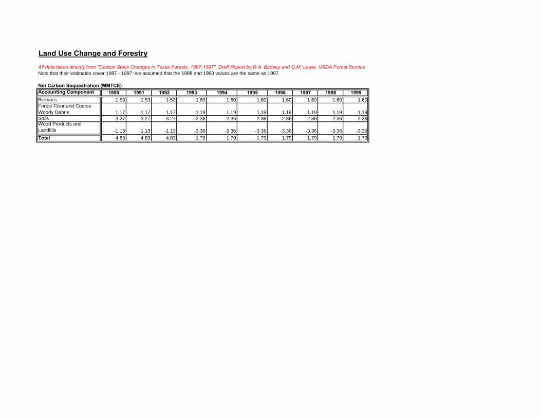
Land Use Change and Forestry

All data taken directly from "Carbon Stock Changes in Texas Forests, 1987-1997", Draft Report by R.A. Birdsey and G.M. Lewis, USDA Forest ServiceNote that their estimates cover 1987 - 1997; we assumed that the 1998 and 1999 values are the same as 1997.

Accounting Component 1990 1991 1992 1993 1994 1995 1996 1997 1998 1999

Biomass 1.53 1.53 1.53 1.60 1.60 1.60 1.60 1.60 1.60 1.60Forest Floor and Coarse Woody Debris 1.17 1.17 1.17 1.19 1.19 1.19 1.19 1.19 1.19 1.19Soils 3.27 3.27 3.27 2.36 2.36 2.36 2.36 2.36 2.36 2.36Wood Products and Landfills -1.13 -1.13 -1.13 -3.36 -3.36 -3.36 -3.36 -3.36 -3.36 -3.36Total 4.83 4.83 4.83 1.79 1.79 1.79 1.79 1.79 1.79 1.79

Net Carbon Sequestration (MMTCE)

Section 2. State Global Warming Plans

A. Summary of State Planning Actions

The TNRCC staff reviewed plans and reports from 15 states and a resolution from the New EnglandConference of Governors regarding potential strategies to reduce greenhouse gas emissions. Ingeneral these Greenhouse Gas Action Plans appear to be written for one of two reasons: 1) the statewanted to be prepared in the event the Kyoto Protocol was implemented or the federal governmentimposed formal restrictions on greenhouse gas emissions, or 2) the state participated in an EPA-sponsored project in which states received funding and guidance to create a greenhouse gas registryand develop an action plan. Seven states participated in the EPA-sponsored program. The majorityof the plans were contracted out to local state universities. Others were written either by the stateenvironmental agency or the state department of energy.

Participation is voluntary in almost all of the suggested strategies of the greenhouse gas action plans. The only exceptions appear to be policies that were already in place addressing other problems whichhappen to reduce greenhouse gases as well.

Five of the plans focus heavily on energy efficiency as a way to reduce carbon dioxide emissions. Inmost states the burning of fossil fuels for generating electricity or to fuel automobiles account for atleast one third of the total greenhouse gases that are emitted annually. The most common mitigationpolicies are listed below:

• Home Energy Rating System• Energy Efficiency Audits• Energy-efficient Mortgage Programs• Model Energy Codes (MEC)• Tax Incentives for Fuel Switching, Cogeneration Projects• Renewable Portfolio-Standards• Emissions Trading• Methane Reclamation Programs• Recycling Programs• State Alternative Fuel Fleets• Truck to Train Mode Shift• Revenue Neutral Tax Incentives• Afforestation

Many states including California are also deregulating utilities in an effort to increase marketcompetition. California predicted that, within four years of deregulation, consumers would begin touse less electricity. These states cite deregulation as a way to reduce greenhouse gases.

To our knowledge, two states enacted formal legislation to reduce greenhouse gases. Massachusettsand Oregon both passed bills that cap carbon dioxide emissions in new power plants, but provideoptions to exceed the cap. Other states have gone in the other direction, issuing bills that urgeCongress and the President not to ratify the Kyoto protocol or that prohibit policies that mandategreenhouse gas reduction.

Following are summaries of the reports:2-1

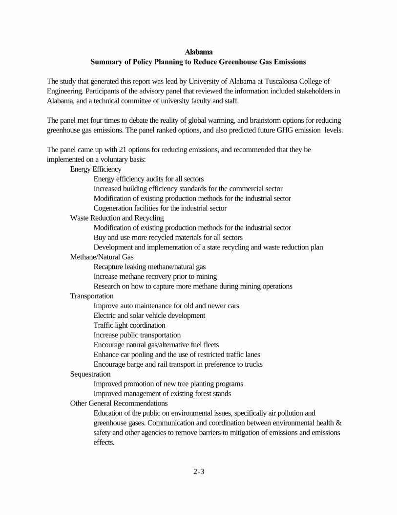
AlabamaSummary of Policy Planning to Reduce Greenhouse Gas Emissions

The study that generated this report was lead by University of Alabama at Tuscaloosa College ofEngineering. Participants of the advisory panel that reviewed the information included stakeholders inAlabama, and a technical committee of university faculty and staff.

The panel met four times to debate the reality of global warming, and brainstorm options for reducinggreenhouse gas emissions. The panel ranked options, and also predicted future GHG emission levels.

The panel came up with 21 options for reducing emissions, and recommended that they beimplemented on a voluntary basis:

Energy EfficiencyEnergy efficiency audits for all sectorsIncreased building efficiency standards for the commercial sectorModification of existing production methods for the industrial sectorCogeneration facilities for the industrial sector

Waste Reduction and RecyclingModification of existing production methods for the industrial sectorBuy and use more recycled materials for all sectorsDevelopment and implementation of a state recycling and waste reduction plan

Methane/Natural GasRecapture leaking methane/natural gasIncrease methane recovery prior to miningResearch on how to capture more methane during mining operations

TransportationImprove auto maintenance for old and newer carsElectric and solar vehicle developmentTraffic light coordinationIncrease public transportationEncourage natural gas/alternative fuel fleetsEnhance car pooling and the use of restricted traffic lanesEncourage barge and rail transport in preference to trucks

SequestrationImproved promotion of new tree planting programsImproved management of existing forest stands

Other General RecommendationsEducation of the public on environmental issues, specifically air pollution andgreenhouse gases. Communication and coordination between environmental health &safety and other agencies to remove barriers to mitigation of emissions and emissionseffects.

2-3

A possible tax on carbon emissions was considered but rejected due to the economic depression thatmight result from this action.

In 1998, Alabama House Bill 465 prohibited the passage of any state regulations before the Kyotoprotocol has been ratified. The same year Senate Joint Resolution 23 was signed urging PresidentClinton not to sign the Kyoto protocol. The Alabama Greenhouse Gas Reduction Plan was producedthrough a contract but was never adopted by the state government.

The full 150 page report can be obtained by contacting The University of Alabama, Tuscaloosaphone (205)348-8401 fax(205)348-9659.

2-4

CaliforniaSummary of 1997 Greenhouse Gas Emissions Reductions Strategies

The California plan was written in 1997 by the California Energy Commission, when the state wasundergoing restructuring of its energy market, the plan speculates on what effects the restructuring willhave on energy use and CO2 emissions.

Residential and Commercial Emissions Reduction Strategies• State speculates that restructuring will foster uncertainty and reluctance to participate in

new energy efficiency programs.• When market stabilizes after four years, they will market efficiency programs and

participation will increase.Industrial Emissions Reduction Strategies: Voluntary Programs

• Currently no regulation governing industrial CO2 emissions. • Voluntary programs to reduce emissions include National Industrial Competitiveness

through Energy, Environment and Economics Program; Motor Challenge Program;Industrial Assessment Centers, and the Climate Wise Program.

• Current efforts are to make information on the programs more availableAlternative California Oil and Natural Gas Production Technologies

• Strategies to enhance oil and gas recovery have focused on economics and newtechnology.

• Three new methods for recovering oil show potential for less waste: thermal enhancedoil recovery, chemical enhanced oil recover, and gas displacement methods.

Electric Generation Emissions Reduction Strategies• Focused on: 1) the need to account for environmental externalities and incorporation

their values in resource planning and procurement, 2) promoting high-efficiency gasgeneration, and 3) promoting the development and integration of renewable generationtechnologies.

High Efficiency Gas Generation Technologies• High efficiency gas generation systems are under development and hold promise for

significantly improved fuel efficiency.Strategies for Developing and Integrating Renewable Generating Technologies

• Renewable sources currently used include solid fuel biomass, geothermal, wind, smallhydroelectric, solar, and municipal solid waste.

• State wants to expand efforts to accelerate renewable energy technology throughresearch, development, demonstration, and commercialization.

Forestry Management for Carbon Sequestration and Emissions Reductions• Improved forestry management will create better carbon sequestration.• Current programs include California Forest Incentive Program and wildlands

management.

2-5

• Private landowners need to be induced to participate in land management programs.• Statewide biomass program should be reinstated.• Encourage planting of urban trees, since they sequester 15 times more CO2 than forest

trees.Livestock Management for Methane Emissions Reductions

• Represents California’s second largest source of emissions• Efforts to develop, commercialize and package off-the-shelf systems for small scale

anaerobic fermentation of manure to produce biogas.• Work continues to research, develop, demonstrate, and evaluate technologies to

recover methane from livestock and other organic waste.Solid Waste Management for Methane/CO2

• Integrated Waste Management Board has set a goal of 50 percent landfill diversion by2000.

• The state implementation plan calls for re-evaluation of current management of municipal solid waste.

• Cost-analysis should be done for sale of marketable materials from methane sourcereduction.

Transportation• Policies currently in progress include increasing vehicle fuel efficiency, increasing non-

highway transportation efficiency; developing alternative fuels, vehicles and markets;promoting biomass based alcohol fuels, electric vehicles and hydrogen fuels; andincorporating long-term transportation needs into land use planning.

AFV Strategies• Fuel taxes based on carbon content, national taxes would be more effective than state

taxes. • Development of better alternative fuel vehicle technology and infrastructure.• Higher fuel economy standards and fee rebates are effective at reducing CO2.• Expanding HOV lanes and more monetary incentives for AFV should be enacted.

Land Use and Transportation Planning• Regional and local governments must plan more effectively to meet long term

transportation needs.• Results are mixed on the effectiveness of regulations, programs, and measures to

reduce personal vehicle use, numbers of vehicles trips, vehicle miles traveled, and trafficcongestions. Plan calls for a combination of strategies1.

California reported a reduction in energy use in the spring of 2001 following shortages and blackouts. All policies in the 1997 California climate change plan are considered voluntary.

The full 172 page report can be obtained online at:www.energy.ca.gov/global_climate_change/report.html, or by contacting the California EnergyCommission.

2-6

DelawareSummary of Climate Change Action Plan

The Delaware action plan, written in January 2000 by the University of Delaware, was sponsored bythe Delaware State Energy Office and the US EPA. By 2010, state CO2 levels will be 22percent morethan 1990 without reduction action. The Delaware Climate Change Committee designed the plan toreduce greenhouse gas emissions by 7 percent from current emissions. The Action Plan will generallycost about 3 to5 cents per kilowatt hour saved.

Industrial SectorIndustrial emissions can be reduced by

• Technology upgrades. • Operation and maintenance changes. • improved facility management.

Energy efficiency and savings • Boiler and steam systems. • Heat recovery and containment. • Update motors. • Lighting.

Residential/Commercial Sector• Higher efficiency appliances and lighting • Switching to more efficient fuels, such as natural gas for heating and cooking, • Building-integrated solar cells

Transportation Sector• Fuel efficiency improvements. • Alternative fuel vehicles. • Transportation control measures that reduce the number and length of trips. • Ridesharing, greater use of public transit. • Development planning that reduces urban sprawl.

Utility Sector• Reductions in energy usage by residential, commercial, and industrial users.• Requirement that 1 percent of power generation will come from renewables.• Switching Delaware’s coal fired power plants to natural gas.

Waste Reduction• Waste reduction and recycling programs. • Reduce resource usage.

2-7

Forest Protection• Planting additional trees and protecting existing forests.

This plan does not have mandatory controls or regulations. Participation is voluntary. It includesdiverse ideas thought up by a consortium of climate change experts, but does not necessarily reflect theideas of any individual, committee, or state or federal agency, which the members of the consortiumrepresent.

To obtain a copy of the full 210 page report, contact the Center for Energy and Environmental Policy,University of Delaware or view it online at: http://www.udel.edu/ceep/reports/deccap/deccap.htm.

2-8

Hawaii Climate Change Action Plan

This report was generated in 1998 by the state Department of Business, Economic Development incooperation with other state agencies, to respond to fears that Hawaii might become “less of aparadise” due to the negative results of global warming. The Climate Change Action Plan was writtennot with specific reduction goals in mind but to act as a catalyst for further discussion. If the Kyotoprotocol had been implemented, it was Hawaii’s ambition to get a head start on any actions that wouldneed to be taken.

The plan recommends that Hawaii reduce emissions; identify future effects on people, the environment,ecosystems and the economy; and develop a long range plan.

Greenhouse gas emission sources were divided into the following sectors:• Transportation energy 42 percent.• Electricity generation 41 • Municipal waste 7• Industrial energy 4• Agriculture 3• Commercial energy 1• Residential <1• Industrial process <1The breakdown does not take into account emissions from jet fuel from intra and inter-island flights. Those flights are considered “essential to tourism and the well being of [Hawaii’s] people.”

The plan predicts that without action, emission levels (in carbon equivalents) will increase to 20 percentover 1990 levels by 2010 and 33 percent by 2020. Several scenarios focused on the energy sectorand were modeled to explore mitigation strategies, but none reached the Kyoto targets by 2020.Somerecommended methods for reducing GHG emissions are listed below according to sector:

Transportation Energy

Ground transportation Increase visibility of driving costs.

Publicize incentives for owning alternative fuel vehicles.

Increase use of mass transit.

Air transportation Adopt operating measures for fuel efficiency.

Re-equip inter-island airlines with newer, more efficient aircraft.

Examine ways to increase load factors, especially on inter-island flights.

Marine Consider changes in operation procedure for energy efficiency.

Adopt technical improvements to ships.

Improve data collection for use in estimating future marine fuel use.

2-9

Electricity

Crosscutting actions Continue efforts to restructure Hawaii’s electric utilities.

Enhance utility participation in Climate Challenge Program.

Set a Renewable Energy Portfolio Standard and a max for GHG emissions.

Demand-sidemanagement

Expand state government energy performance contracting.

Make buildings that are appropriate to local climate to reduce energy.

Participate in US government energy efficiency programs.

Supply-side activities Maximize cost-effective cogeneration.

Increase use of solar water heating.

Determine capability of electric utility systems to use intermittent renewableenergy.

The full 200 page report can be viewed online at: http://www.hawaii.gov/dbedt/ert/ccap/ccap-toc.htmlor a copy can be obtained by contacting Hawaii’s Department of Business, Economic Development &Tourism.

2-10

Illinois Climate Change Action Plan

The action plan was produced in 1994 by the four year-old climate change task force, created by theGeneral Assembly in Joint House Resolution 81. The report stresses that Illinois must act on globalclimate change issues now.The task force found five key issues that were of importance to Illinois:

• What are the economic, social, physical, and environmental implications of climatechange for Illinois?

• How does the national global climate change policy concern Illinois?• What are the appropriate global change mitigation strategies for Illinois?• What adaptive responses to global climate change can Illinois take?• How can climate change research, monitoring, and education in Illinois be enhanced?

Expecting a goal of reducing emissions to 1990 levels to be set of recommended by the federalgovernment, Illinois set itself to comply with that goal by using strategies that would work for Illinoisrather than waiting for the federal government to impose mandatory reduction measures.

In order to reduce emissions to 1990 levels by 2000, reductions and sinks will have to amount to atleast 10 million tons of carbon equivalents. To do that, the task force came up with the followingstrategies:

• Implement energy efficiency and conservation programs and assist Illinois companies inmeeting their federal climate change emissions reduction commitments.

• Expand the state’s rural and urban tree planting and forest management assistance programs as cost-effective measures to augment Illinois’s greenhouse gas sink.

• Test the cost-effectiveness of joint implementation for long-term emissions reduction andsupport the U.S. Initiative on Joint Implementation.

• Assist US DOE and USEPA in improving and implementing the Climate Change Action Plan to ensure that it addresses issues important to Illinois

In order to address the issue that there is not enough state focused climate monitoring and appliedresearch on climate impacts, the follow strategies were suggested:

• Enhance support to the Climate Change Program at the State Water Survey and designate benchmark weather station for climate change monitoring.

• Urge the federal government to emphasize applied research and to direct more funding tothe state and regional levels in its research priorities.

• Assist Illinois researchers in securing funds for studies of weather-sensitive natural resources and human activities and fund regional integrated assessments of impacts.

2-11

The plan also recommended the following strategies to prepare the state of Illinois to deal with anypossible effects of climate change:

• • Revise state water laws to deal with water issues in times of scarcity and establisha state water entity to deal with water shortage emergencies.

• • Develop rules that require consideration of climate change in the design andconstruction of the state’s infrastructure.

• • Fund a climate change program to develop educational materials, provideincentives for inclusion in curricula, and support a speakers bureau.

A copy of the full report can be viewed online at http://dnr.state.il.us/orep/inrin/eq/iccp/toc.htm or a hardcopy can be obtained by contacting Illinois Department of Energy and Natural Resources, Office ofResearch and Planning.

2-12

Iowa Greenhouse Gas Action Plan

The State of Iowa generated an action plan in 1996, for mitigation of greenhouse gases as part of a three-phase program. The first phase called for the creation of a greenhouse gas inventory, the second phasewas the creation of the action plan, and the third is the evaluation and documentation of the reductionsstrategies from phase two. The report was contracted to the University of Iowa and funded by the EPA.

At the time of the report Iowa was the 15th highest emitter of greenhouse gases per capita (all gasestogether measured in carbon equivalents), with 29 tons of carbon dioxide per Iowan. Without anymitigation action, by 2010, emissions will be up 18.5 percent from 1990 levels. Implementing the priorityoptions of the plan would decrease emission by 84 million tons of carbon equivalents annually.

The plan initially considered 34 strategies, then recommended the top 16 which are listed on the secondpage. In addition to reducing greenhouse gases, implementation could save the state $300 million annuallythrough reduced energy costs and another $32 million from avoided emissions.

Reduction Strategies for Carbon Dioxide

Priority MaximumSector Recommended Options to Reduce Reductions Feasible

Greenhouse Gas Emissions (In MTCE/y) Reduction

Agriculture • Reforestation of marginal lands 2.7 13.5• Production of energy crops 0.09 0.26• Reduction of nitrogen fertilizer 0.4 0.4• Reclamation of methane gas at 0.1 0.7 large hog lots (more than 5,000 head)• Continued improvement of farm 0.1 0.1 efficiency

Transportation • Improve vehicle fleet efficiency 2.9 4.1• Discourage single occupancy trips 0.18 0.36

Utility • Carbon dioxide emissions inventory 1.4 2.1• Wind power development 0.28 0.56• Demand-side management 0.2 1.0

(voluntary)• Emissions trading 2.0 3.5

(Market based)

2-13

Commercial/ • State voluntary programs .08 0.2Industrial (Iowa Energy Bank, Rebuild Iowa, Total

Assessment Audit, Climate Wise)• Federal voluntary Programs 2.1 4.2• Emissions trading 2.0 3.4

(Market based)• Carbon dioxide emissions inventory 1.4 2.0

Residential • State and federal voluntary programs 0.67 1.3

The full 79 page report can be viewed online at http://www.cgrer.uiowa.edu/research/reports/iggap/, or ahard copy can be obtained by contacting the Iowa Department of Natural Resources.

2-14

Climate Change Mitigation Strategies for Kentucky

The plan was written by Kentucky Division of Energy in June of 1998 with funds provided by the USEPA. All proposals brought forth by the plan were designed to meet two criteria: 1) policies should notbe to costly, and 2) they must be flexible.

If the following policies were fully implemented the resulting reductions would put greenhouse gasemissions in Kentucky back at 1990 levels:Residential Enforcement of building codes

Home energy rating systemSolar heating for low temperature applicationsSolar electric systems

Commercial Enforcement of building codesEnergy efficiency in government buildingsSolar heating for low temperature applicationsSolar electric systems

Industrial Expanded IAC/KPPC programsSolar heating for low temp. applicationsRecovery of HFC-23 byproductsCoal-bed methane recovery

Transportation Feebates for fuel efficient vehiclesUtilities Shift coal to gas (NGCC/IGCC/AFT)Agriculture Manure managementCarbon Urban forest management programssequestration Rural forest management programs

The plan also found other options that could be used to reduce emissions:• Improvements in forest management and timber production leading to increased rates of carbon

sequestration.• The use of clean coal technologies and natural gas to generate electricity, replancing a number of

existing conventional coal power plants.• Reduction of the emissions of chlorofluorocarbon manufacturing byproducts;• Improved end-use efficiency in the industrial sector.• Improved construction practices and enforcement of energy-related building codes in the

commercial and residential sectors.

Kentucky Senate Bill 300 was signed in 1998 to prohibited any regulation or permit conditions that mightlimit greenhouse gas emissions unless authorized by the General Assembly or by federal statute.However, the bill does not prohibit any voluntary initiative to reduce greenhouse gas emissions.

The full report can be viewed at:http://www.epa.gov/globalwarming/publications/actions/state/ky_2_fin.pdf or by contacting Geoff Youngat the Kentucky Division of Energy.

2-15

State of Maine Climate Change Action Plan

This report was generated in 2000 as part of a three-phase program dealing with climate change, andfunded by the USEPA. The report does not reflect the official opinion of the state or any agency, but isbased on scientific knowledge and the opinion of Maine’s climate change task force. The task force’sgoal was to prepare a report that would stimulate discussion and debate among the public.

The task force identified three areas that need to be addressed with regards to climate change.• The first is to figure out the science of it, will most scientific work recognizes that the balance of

evidence points to humans having a significant impact on climate, some critics argue that theevidence is misleading and greenhouse gases can benefit the world..

• The second area is vulnerability. Maine’s coastlines are threatened as well as its large tourism andrecreation sectors. Tropical diseases could move northward is climate is warmed. Maine is alsovulnerable to federal policies that could compromise the economy of the state.

• The last area of focus is policy. Federal laws call for a voluntary approach to mitigation.

The plan identified two responses to climate change, one is action towards abatement of greenhouse gasemissions and the other is preparation to respond to the warming of the climate.

The following is a summary of the main points put forth by the report:• Investment in greenhouse gas mitigation is a form of risk reduction and is prudent public policy.• A starting place for further discussion and policy refinement in the public and private sectors.• Goals can be achieved in part though expansion or completion of existing state and federal

programs.• Take economic advantage of potential future federal policies to limit greenhouse gas emissions.

The following are the actions recommended by the plan to mitigate emissions of greenhouse gases listedby area:Vision and Leadership: Establish in state government a senior climate change administrator to direct,coordinate, and implement the Climate Change Action Plan.Public Information and Education: Create an education coordination council to increase publicawareness of the risks and potential consequences of global climate changes and the actions that can betaken to lower the risks by such means as energy conservation, motor fuel efficiency, alternative energyapplications, and other actions.Energy Conservation and Efficiency. Promote and support alternative energy technologies and fuels inresidential, public, commercial, and industrial end-use sectors.

2-17

Alternative Fuels and Technologies. Promote and support energy conservation and efficiency inresidential, public, commercial, and industrial end use sectors.Business Opportunities and Competitiveness. Identify and capture business opportunities in the fieldof environmental technologies and services based on alternative fuels applications, energy conservationtechniques, and newly emerging research in CO2 control and management technologies and practices. Transportation. Implement state transportation plans that reduce fuel consumption, and promote energyefficient traffic and freight movement. Support energy efficient patterns of development, and supportalternative models of transportation.Electricity Generation. Work to reduce electricity demand through energy conservation measures andto shift electricity generation to lower or non-carbon fuels, such as solar, wind, and hydropower. Improveconsumer ability to choose low or no-emission sources of electricity supply.Environmental Protection and Improvement. Gain greenhouse gas reductions as a cobenefitassociated with the implementation of existing and new environmental protection and managementprograms, especially in air quality control and solid waste management. Consider the use of generationperformance standards, emissions credit trading, and carbon storage offsets.Land Use and Resource Management. Work to promote and support land use and resourcemanagement practices that reduce or avoid the net release of greenhouse gases into the atmosphere.Incorporate carbon dioxide storage considerations into forest and agricultural management programs.Encourage patterns and densities of development that will support efficient use of energy resources.Monitoring and Adaption. Create an environmental monitoring network that can detect changes in keyenvironmental conditions and allow timely adaptive actions, including reduction of risk to human healthand disruptions in economic and ecological systems.Waste Management and Recycling. Increase the reuse and recycling of materials to avoid emissionsof greenhouse gases associated with manufacturing new products from virgin materials.

The full 57 page report can be viewed online at http://janus.state.me.us/spo/CCAP/index.htm, or a hardcopy can be obtained by contacting the Maine State Planning Office.

2-18

New England Governors/Eastern Canadian PremiersSummary of Climate Change Action Plan, August 2001

In July 2000 the Conference of New England Governors and Eastern Canadian Premiers adopted aresolution on global warming. The Conference directed the Committee on the Environment and theNortheast International Committee on Energy to hold a workshop, evaluate the conclusions, and write arecommended action plan.

The workshop identified many opportunities to promote greenhouse gas reductions and possible adaptionmeasures while still meeting other governmental goals, including: • shifting to less polluting energy resources; • maximizing effectiveness of energy conservation; • promoting technologies which reduce the use of fossil fuel; • actions to maintain a greater share of energy dollars within the region; • actions to support agriculture, fisheries, timber, etc. to adapt to climate impacts; • encourage similar actions by fellow states; • design and build new infrastructure to minimize impacts of climate change; • preserving green spaces including forests and farm lands; • creating new jobs in the area of energy efficiency and renewables; The plan also identified a short-term goal to reduce regional GHG emissions to 1990 levels by 2010, amid-term goal to reduce GHG emissions by at least 10% below 1990 levels by 2020, and a long-termRegional Goal to reduce regional GHG emissions sufficiently to eliminate any dangerous threat to theclimate; current science suggests a reduction of 75 to 85% below current levels.

The plan included nine Action Items with 34 individual recommendations for the New England States andEastern Canadian Provinces:1) Establish a Regional Standardized GHG Emissions Inventory;2) Establish a Plan to Reduce GHG Emissions and Conserve Energy;3) Promote Public Awareness;4) State and Provincial Governments Should Lead by Example;5) Reduce Greenhouse Gases from the Electricity Sector;6) Reduce Total Energy Demand Through Conservation;7) Reduce the Negative Social, Economic and Environmental Impacts of Climate Change;8) Decrease the Growth GHG emissions from the Transportation Sector;9) Create a Regional Emission Registry and Explore a Trading Mechanism.

A copy of the 18 page report can be obtained by contacting the New England Secretariat, New EnglandGovernors’ Conference Inc., 76 Summer St., Boston, MA 02110

2-19

New Jersey Greenhouse Gas Action Plan

In 1998 the New Jersey Department of Environmental Protection issued an administrative order setting avoluntary goal of reducing greenhouse gas emissions to 3.5 percent below 1990 levels by 2005. TheNew Jersey Greenhouse Action Plan was then written in 2000 by the New Jersey Climate ChangeWorkgroup within the NJ DEP. The action plan outlines strategies that will be cost effective, reducegreenhouse gas emissions, and are ready for implementation. The strategies will be reviewed and updatedperiodically, initially every six months, to make sure New Jersey is on the right track with regards toemissions reductions.

The major sources of greenhouse gases are residential and commercial buildings, industrial operations,and transportation. Three general ways to deal with these sectors, as outlined by the plan, are:

• generate energy using sources that produce less greenhouse gases.• employ more efficient means of fuel consumption so less energy is used to perform the

same tasks.• capture some of the wasted energy for productive use.

Some of the more specific actions recommended by the plan are broken down by sector below.

Residential BuildingsIncrease rate of residential electric appliances upgradesImprove efficiency by updating building codes and use of the Energy Star Building Prog.

Commercial BuildingsIncrease rate of Space heating tune up to reduce non electric fuel useIncrease lighting upgrade and office equipment to Energy Star level

Industrial OperationsIncrease rate of undertaking steam distribution and trap repair programsIncrease rate of maintenance to air compressor systemsUse of more variable speed drives for high use motors

TransportationImplement an Inspection/Maintenance Program for New Jersey registered vehiclesIncrease improvements to mass transit to reduce number of automobiles

Municipal Solid WasteRecycling to keep organic material out of landfills and avoid methane releasesFlare methane to change it to CO2

Natural ResourcesIncrease new woody tree growth

The full 113 page report can be viewed online atwww.epa.gov/globalwarming/publications/actions/state/nj_actionplan.pdf or by contacting the NewJersey Department of Environmental Protection.

2-21

North Carolina State Action Plan for Reducing Greenhouse Gas Emissions

This plan was written in 2000 by Appalachian State University through a contract with North CarolinaDepartment of Commerce, and funded by EPA. It was developed so that North Carolina would havesome idea of the action that would need to be taken if the United States were to adopt the Kyotoprotocol. The plan is designed to make good economic sense, utilize both old and new emissionsreduction strategies and technologies, and to involve greater efficiencies and conservation to reduceemissions. EPA’s greenhouse gas emissions software was used to generate outcome models. Torrie SmithAssociates adapted the software to be used at a state level and North Carolina was one of the initialtesters.

The following are the strategies explored by the plan and modeled by the greenhouse gas software:

Strategies Reductions in MMTCEIndustrial Sector

Energy efficiency improvements 7.44Modernized manufacturing processes 2.57New machine technology 3.18Automation 1.72Fuel switching: coal to natural gas 0.64Switching to renewables 1.14

Commercial SectorExisting buildings:

Update and enforce efficiency standards for existing buildings 2.13Fuel Switching:

Switch from electricity to solar or natural gas for heating 0.46New Buildings:

Improvements in thermal efficiency, HVAC efficiency,alternative energy options, and hot water efficiency 2.28

Residential SectorAppliances and equipment, upgrade efficiency of lighting, HVAC, efficiency 1.35Solar water and space heating 0.19Update efficiency of old building 6.14

TransportationMetropolitan car/van pooling and public transport 0.06Increase fuel efficiency through speed limits and CAFÉ standards 0.27Per capita vehicle miles traveled (VMT) target 4.08Road pricing strategy 0.05VMT fees 3.76Fuel tax 3.76VMT based land use 0.03

AgricultureMethane management and recovery system and better farm management 0.1

2-23

ForestryIncrease forest area by 10 percent 4.95Improve forest area management unknownRecycling paper and wood products 2.74Encourage use of wood residues for products and fuel unknown

The full report can be viewed online at:http://www.geo.appstate.edu/bulletin/EPA_projects/NCaction/intro.html or contact Appalachian StateUniversity, Department of Geography and Planning for a hard copy.

2-24

Oregon Climate Change Action Plan

In 1992 Oregon’s Progress Board set a benchmark to stabilize CO2 emissions, but later realized thatreaching that goal would be harder than anticipated. The action plan was written in 1999 by the stateDepartment of Energy and funded by the EPA. It proposed extending state policy to use efficiency andrenewable resources to meet the state’s energy needs and reduce GHG emissions.Oregon currently has in place programs promoting energy efficiency, renewable energy, integrated energyplanning, and land use and transportation planning, but CO2 emissions are still projected to increase asmuch as 32 percent. The Oregon Department of Energy is not recommending any actions that wouldstabilize emissions in this report and in particular no actions that reduce emissions from transportation.The following policies would, if implemented, reduce emissions by 2 million tons by 2015.

Energy Efficiency and Renewable Resources• Capture all conservation and renewable resources at cost-effectiveness levels that include cost for

CO2 emissions• Maintain consideration of greenhouse gas emissions in energy resource plans and facility siting

Transportation Efficiency• Increase the efficiency of Oregon’s transportation system to reduce the state’s reliance on oil to

reduce the pollution, congestion, greenhouse gases, and other costs associated with vehicle travel.

• Explore voluntary and market-based incentives for purchasing efficient vehicles. • Promote efficient operation of vehicles.

Offsets• Offset CO2 emissions through planting trees to sequester carbon from the atmosphere and

through other means such as increasing energy efficiency.

Economic Development• Target new technologies for economic development that will contribute most in the future to

furthering state, national, and international climate change goals.

Adaptation to Climate Change• Support research on the effects of climate change on water, fisheries, agricultural, and forestry

resources and on sea level rise on the Oregon coast.

Recycling, Reuse, and Solid Waste Management• Reduce the generation of waste and recycle and reuse materials.

2-25

National Agenda• Focus federal research and development, standards, incentives, collaborations, and promotion

activities to give priority to reducing greenhouse gas emissions, and use pricing mechanisms toincorporate climate change externalities into the marketplace.

In 1997, Oregon passed House Bill 3283 which caps CO2 emissions from new utilities at 17 percentbelow the level that the most efficient plant currently emits, and charges a fee for every ton that is emittedabove the cap.

The full 48 page report can be viewed online at www.energy.state.or.us/climate/gggase.htm or a hardcopy can be obtained by contacting the Oregon Department of Energy.

2-26

Tennessee Greenhouse Gas Mitigation Strategies

This plan was developed in 1999 by the Tennessee Technological University, for the TennesseeDepartment of Economic and Community Development with the philosophy that citizens, businesses, andgovernments of Tennessee should and will voluntarily reduce greenhouse gas emissions or increasesequestration because of the economic opportunities in it. The plan recommends that early action creditsshould be established immediately to encourage voluntary reductions.

The report focuses on energy efficiency in residential, transportation, commercial, industrial, utility use,and also on carbon sequestration.

The utility sector produces the majority of greenhouse gases in Tennessee. Through a partnership with theUS Department of Energy, Tennessee is working to reduce those emissions. All other sectors haveprograms that encourage voluntary participation by citizens and businesses.

Some examples of policy recommendations are:Residential: • Promote the replacement of incandescent lighting with compact fluorescent lamps

in existing houses and apartments in Tennessee.• Enact new requirements on the minimum insulation levels and window types for

new residential and apartment construction.Commercial: • Promote and encourage the replacement of inefficient water chillers.

• Promote efficient refrigeration systems for supermarkets.Industrial: • Encourage participation by the industrial sector in federal government sponsored

energy conservation programs.• Promote a detailed energy efficiency enhancing program to assist Tennessee’s

industries in identifying and implementing energy conservation projects.Transportation: • Promote commuter rail alternatives.

• Promote telecommuting, HOV lanesUtility: • Signed a Climate Challenge Participation Accord with DOE to reduce greenhouse gas

emissions by 14.9 million tons of CO2 equivalents below the emissions that would haveoccurred in 2000. They will do this by switching from traditional coal fired units tonuclear, and biomass cofiring units; demand side management programs, improvedefficiency on fossil fuel units and other upgrades.

The full 200 page report can be viewed online at http://www.state.tn.us/ecd/energy_init.htm or a copycan be obtained by contacting the Tennessee Department of Economic and Community Development.

2-27

Fueling Vermont’s Future A Comprehensive Energy and Greenhouse Gas Action Plan

Fueling Vermont’s Future was written in 1998 by the state’s Department of Public Service with theoutlook that Vermont could lead the nation in sound energy use if the bold new policies that wereresearched, modeled, and recommended in this Plan, were implemented. To make serious progress, thestate should take action first in the areas that can produce the greatest impacts. Those areas are:

• Capturing more energy savings in new and existing homes and multi-family low incomehousing.

• Increasing the use of renewable energy sources.• Improving the rate of energy use for transportation.• Reviewing energy policy and taxation at the state and federal levels to assure that energy

goals are promoted.

Working toward an adequate, reliable, secure, and sustainable energy supply will ensure that the acontinued source of energy will keep up the quality of life for all future Vermonters.All in all the report puts forth 120 recommendations for controlling energy use.It sets nine goals for that are part of Vermont’s energy policy: safety, adequacy, reliability, security,sustainability,, environmental soundness, efficiency, affordability, and economic vitality.

If a comprehensive set of policies were implemented in Vermont, the following energy savings could beachieved:

• total energy use reduced by 552 TBtu or 16 percent• oil use reduced by 483 TBtu or 30 percent• non renewable energy use reduced by 750 Tbtu or 26 percent• energy costs reduced by $6.2 billion or 15 percent• air emissions cost on the environment reduced by $5.0 billion or 26 percent• greenhouse gas emissions reduced by 53.3 million CO2 equivalent tons or 21 percent

There are two versions of the report: Volume I is a summary (200 pgs). Volume II is morecomprehensive and both can be viewed online at: http://www.state.vt.us/psd/dpslibrary/cepguide.htm orby contacting the Vermont Department of Public Service.

2-29

Washington State Greenhouse Gas Mitigation Options

This report was created by the Washington State Energy Office, as part two of a two part studysponsored by the US EPA. Phase I was to create a GHG inventory which used current trends to projectemissions to 2010. The second phase was to create an action plan. The funding for the project came froma US EPA state grant program that was initiated in response to the 1993 goal, set by President Clinton,for returning the United State to 1990 GHG emissions levels. The following is a summary of the plan’s suggested policies by sector:Residential Sector

Existing Home Retrofits Direct use of natural gas in buildings Minimum R-values for attics, walls, floors, and duct insulationLow flow shower heads Hot water tank upgradeCaulking joints Fluorescent lighting upgradesNew Home Building Practices Minimum R values for floors, attics, and walls

Commercial Sector -Efficient fluorescent lighting retrofitsMore efficient food refrigerationA variety of efficiency improvements for public sector commercial buildings

Industrial Sector -Petroleum refining process improvementsPulp and paper process improvementsAluminum process improvements

Transportation Sector -Tire pressure checksMore efficient airplane enginesGas tax ($1.00/gallon)Vehicle mileage taxFee rebates ($100/miles-per-gallon off baseline)Parking restrictionsDiesel to electric train conversionTruck to train mode shift

Generating Resources - Chemical boiler cogenerationLandfill gas combustionAnimal manure managementNuclear powerWood waste combustionAgricultural waste combustionWind power

2-31

Carbon Sequestration -Afforestation

This report was prepared for the EPA, but all suggestions are just that, and neither the state ofWashington nor the EPA “make any warranty, express or implied, or assume any legal responsibility forthe accuracy, completeness, or usefulness of any information, apparatus, product, or process disclosedwithin this report.”

In 2000, House Bill 5121 passed the Senate. It established a carbon storage program as an economicincentive to maintain long-term forest production.

The full report can be viewed online at:http://www.epa.gov/globalwarming/publications/actions/state/wa/mitigatea.html#Table1 or a copy canbe obtained by contacting Nicolas Garcia at the Washington State Energy Office.

2-32

Wisconsin Greenhouse Gas Emissions Reduction Cost Study

The Wisconsin Department of Natural Resources has lead four studies relating to greenhouse gasemissions. The first, in 1993, was an inventory that quantified the current greenhouse gas emissions in thestate. The study’s results were released in a report that same year. The second study projected emissionestimates to 2010 and found that there would be a 28 percent increase in greenhouse gas emissions from1990 levels if no actions were taken. The third study in 1998, resulted in the action plan. It looked atpotential reduction measures and quantified the associated costs. The forth study explored the effects ofimplementing the action plan on the economic investments of Wisconsin.

The studies found that utilities produced the most GHG emissions, but that focusing on electricity users aswell as producers would create the biggest reduction. The following energy efficiency measures wouldresult in a reduction of 35 million tons of carbon dioxide by 2010:• replacement of electric appliances, and equipment in all sectors with more efficient equipment. • switching from coal-fired power plants to natural gas.• modest increases in automobile efficiency.Energy efficiency saving would balance out with the increased cost of fuel switching, resulting in a netsavings of $2 million, but not all implementation costs were included in the estimate.

Until policies and treaties are worked out at the international level, Wisconsin recommends implementingwhat they refer to as “no regrets” actions, or actions that over the years pay back the up front costs toimplement them and are relatively easy to implement. The so called “no risk” action would be part of thefirst phase of a multi phase reduction policy. The first phase is designed only to curb the rate of growth of greenhouse gas emissions by encouragingenergy efficient choices using the following methods:• Wisconsin state government leads by example• Vigorously promote voluntary private sector-led initiatives to adopt

energy efficiency measures (including fuel switching)• Provides financial incentives for cost effective energy efficiency measures• Revise or update state building codes to support energy efficiency

improvements.

The second phase could only be implemented once the federal government had agreed with other nationson a target for greenhouse gas emission reductions. Then state and local policies would be evaluated andredirected toward reaching that target.

The 180 page report and appendices can be viewed online at:http://www.dnr.state.wi.us/org/aw/air/global/WICCAP.pdf or by contacting the WisconsinDepartment of Natural Resources.

2-33

C. EPA Guidance Documents for Developing Global Warming Action Plans

The US EPA has published a number of documents which address state planning associated withGreenhouse gas emissions. The State Workbook: Methodologies for Estimating GreenhouseGas Emissions, published in 1992, contains a set of guidelines and methodologies to compile aninventory of greenhouse gas emissions and sinks. EPA indicates that identifying emissionsources and sinks is a critical first step to developing a comprehensive and long range state actionplan. This workbook provides worksheets for calculating greenhouse gas emissions by sourcecategory, along with formulas and alternative approaches and references to additionalinformation. The original State Workbook is available through EPA’s Office of Policy, Planningand Evaluation, Office of Economy and Environment.

The State Workbook was revised several times since the original publication. In 1999, EPApublished EIIP Volume VIII: Estimating Greenhouse Gas Emissions which is available on theInternet at:

http://www.epa.gov/ttn/chief/eiip/techreport/volume08/index.html

Volume VIII was written by the ICF Consulting Group and has not been reviewed or approvedfor publication. It provides emission estimation techniques for estimating carbon dioxide,methane and nitrous oxide emissions from 14 different anthropogenic activities.

In 1998, the EPA also published the States Guidance Document: Policy Planning to ReduceGreenhouse Gas Emissions, Second Edition (EPA #230-B-98-002) which provides supportinginformation to assist policymakers in further understanding the issues associated with climatechange and in identifying and evaluating options to mitigate emissions identified during theinventory process. It also offers suggestions on how climate change programs can concentrate onreducing emissions where the greatest opportunities exist within each individual state. Thisdocument is available on the Internet at:

http://www.epa.gov/oppeoee1/globalwarming/publications/reference/stateguidance/index.html

The EPA also maintains a web page of Online Tools which include interactive Calculators tohelp with estimating greenhouse gas emissions of specific activities and evaluating emissionreduction opportunities. The page includes a link to Software packages available to measure andanalyze energy consumption and emission reduction opportunities. A final section contains realworld Case Studies which may be useful to in comparing emission options against projectsagainst greenhouse gas emissions reduction projects that have been successfully implemented. This page is located at:

http://www.epa.gov/oppeoee1/globalwarming/tools/index.html

2-35

3 - 1

Section 3. Information from State Agencies and Universities on Global Warming.

A. Summary of recent reports1. Climate Change Science, National Research Council. 3-32. Intergovernmental Panel on Climate Change Report. 3-93. Royal Society Report on Sequestration. 3-234. Union of Concerned Scientists Gulf Coast Texas Report. 3-255. Global Warming: A Guide to the Science 3-31

B. Bibliography of recent science reports on global warming. 3-36

C. University Inputs:1. Rice University 3-382. Southwest Texas State University 3-393. Texas A&M University 3-404. Texas Tech 3-425. University of Houston 3-436. University of Texas, Austin 3-44

D. State agency and other contacts1. Texas Department of Aging 3-462. Texas Department of Parks and Wildlife 3-473. Texas Department of Transportation 3-484. Texas General Land Office 3-505. Texas Public Utilities Commission 3-516. Texas Water Development Board 3-527. Lower Colorado River Authority 3-52

3 - 2

Climate Change Science, National Research Council. (June, 2001)This study originated from a White House request to help inform the Administration’s ongoingreview of U.S. climate change policy. In particular, the written request asked for the NationalAcademies’ “assistance in identifying the areas in the science of climate change where there arethe greatest certainties and uncertainties,” A distinguished committee with broad expertise anddiverse perspectives on the scientific issues of climate change was therefore appointed throughthe National Academies’ National Research Council.

Intergovernmental Panel on Climate Change Report. (November, 1997)The Intergovernmental Panel on Climate Change (IPCC) was jointly established by the WorldMeteorological Organization and the United Nations Environment Programme in 1988 to assessthe scientific and technical literature on climate change, adaption to and mitigation of climatechange. Since its inception, the IPCC has produced a series of Assessment Reports, SpecialReports, Technical Papers, methodologies and other products which have become standard worksof reference, widely used by policymakers, scientists and other experts.

This Special Report, which has been produced by Working Group II of the IPCC, builds on theWorking Group’s contribution to the Second Assessment Report (SAR), and incorporatesmore recent information made available since mid-1995. It addresses an important questionposed by the Conference of the Parties (COP), namely, the degree to which human conditionsand the natural environment are vulnerable to the potential effects of climate change. The reportestablishes a common base of information regarding the potential costs and benefits of climaticchange, including the evaluation of uncertainties.

This report was selected to represent international scientific discussion of global climate change.

Royal Society Report on Sequestration. (July and November, 2001)This report evaluates the scientific issues relating to the role of land carbon sinks and seeks toinform the ongoing international debate about their possible use for the mitigation of climatechange.

Union of Concerned Scientists Gulf Coast Texas Report. (October, 2001)This report compiles research from scientists interested in the effects of global climate change. Itis written to inform the public and policymakers. It was selected as an example of the scientificdebate focused on the effects of global climate change on Texas.

Global Warming: A Guide to the Science. (2001)The purpose of this report is to provide information about the complex science involved in policydebates. It was selected as an example which emphasizes uncertainties in the scientific debate.

Committee on the Science of Climate Change

Division on Earth and Life Studies

National Research Council

NATIONAL ACADEMY PRESSWashington, D.C.

CLIMATE CHANGESCIENCE

AN ANALYSIS OF SOME KEY QUESTIONS

1

Greenhouse gases are accumulating in Earth’s atmo-sphere as a result of human activities, causing surface airtemperatures and subsurface ocean temperatures to rise.Temperatures are, in fact, rising. The changes observed overthe last several decades are likely mostly due to human ac-tivities, but we cannot rule out that some significant part ofthese changes is also a reflection of natural variability.Human-induced warming and associated sea level rises areexpected to continue through the 21st century. Secondaryeffects are suggested by computer model simulations andbasic physical reasoning. These include increases in rainfallrates and increased susceptibility of semi-arid regions todrought. The impacts of these changes will be critically de-pendent on the magnitude of the warming and the rate withwhich it occurs.

The mid-range model estimate of human induced globalwarming by the Intergovernmental Panel on Climate Change(IPCC) is based on the premise that the growth rate of cli-mate forcing1 agents such as carbon dioxide will accelerate.The predicted warming of 3°C (5.4°F) by the end of the 21stcentury is consistent with the assumptions about how cloudsand atmospheric relative humidity will react to global warm-ing. This estimate is also consistent with inferences aboutthe sensitivity2 of climate drawn from comparing the sizes ofpast temperature swings between ice ages and interveningwarmer periods with the corresponding changes in the cli-mate forcing. This predicted temperature increase is sensi-

tive to assumptions concerning future concentrations ofgreenhouse gases and aerosols. Hence, national policy deci-sions made now and in the longer-term future will influencethe extent of any damage suffered by vulnerable humanpopulations and ecosystems later in this century. Becausethere is considerable uncertainty in current understanding ofhow the climate system varies naturally and reacts to emis-sions of greenhouse gases and aerosols, current estimates ofthe magnitude of future warming should be regarded as ten-tative and subject to future adjustments (either upward ordownward).

Reducing the wide range of uncertainty inherent in cur-rent model predictions of global climate change will requiremajor advances in understanding and modeling of both (1)the factors that determine atmospheric concentrations ofgreenhouse gases and aerosols, and (2) the so-called “feed-backs” that determine the sensitivity of the climate system toa prescribed increase in greenhouse gases. There also is apressing need for a global observing system designed formonitoring climate.

The committee generally agrees with the assessment ofhuman-caused climate change presented in the IPCC Work-ing Group I (WGI) scientific report, but seeks here to articu-late more clearly the level of confidence that can be ascribedto those assessments and the caveats that need to be attachedto them. This articulation may be helpful to policy makers asthey consider a variety of options for mitigation and/or adap-tation. In the sections that follow, the committee providesbrief responses to some of the key questions related to cli-mate change science. More detailed responses to these ques-tions are located in the main body of the text.

What is the range of natural variability in climate?

The range of natural climate variability is known to bequite large (in excess of several degrees Celsius) on local

Summary

1A climate forcing is defined as an imposed perturbation of Earth’senergy balance. Climate forcing is typically measured in watts per squaremeter (W/m2).

2The sensitivity of the climate system to a prescribed forcing is com-monly expressed in terms of the global mean temperature change that wouldbe expected after a time sufficiently long for both the atmosphere and oceanto come to equilibrium with the change in climate forcing.

2 CLIMATE CHANGE SCIENCE

and regional spatial scales over periods as short as a decade.Precipitation also can vary widely. For example, there is evi-dence to suggest that droughts as severe as the “dust bowl”of the 1930s were much more common in the central UnitedStates during the 10th to 14th centuries than they have beenin the more recent record. Mean temperature variations atlocal sites have exceeded 10°C (18°F) in association withthe repeated glacial advances and retreats that occurred overthe course of the past million years. It is more difficult toestimate the natural variability of global mean temperaturebecause of the sparse spatial coverage of existing data anddifficulties in inferring temperatures from various proxydata. Nonetheless, evidence suggests that global warmingrates as large as 2°C (3.6°F) per millennium may have oc-curred during retreat of the glaciers following the most re-cent ice age.

Are concentrations of greenhouse gases and other emis-sions that contribute to climate change increasing at an ac-celerating rate, and are different greenhouse gases and otheremissions increasing at different rates? Is human activitythe cause of increased concentrations of greenhouse gasesand other emissions that contribute to climate change?

The emissions of some greenhouse gases are increasing,but others are decreasing. In some cases the decreases are aresult of policy decisions, while in other cases the reasonsfor the decreases are not well understood.

Of the greenhouse gases that are directly influenced byhuman activity, the most important are carbon dioxide, meth-ane, ozone, nitrous oxide, and chlorofluorocarbons (CFCs).Aerosols released by human activities are also capable ofinfluencing climate. (Table 1 lists the estimated climate forc-ing due to the presence of each of these “climate forcingagents” in the atmosphere.)

Concentrations of carbon dioxide (CO2) extracted fromice cores drilled in Greenland and Antarctica have typicallyranged from near 190 parts per million by volume (ppmv)during the ice ages to near 280 ppmv during the warmer“interglacial” periods like the present one that began around10,000 years ago. Concentrations did not rise much above280 ppmv until the Industrial Revolution. By 1958, whensystematic atmospheric measurements began, they hadreached 315 ppmv, and they are currently ~370 ppmv andrising at a rate of 1.5 ppmv per year (slightly higher than therate during the early years of the 43-year record). Humanactivities are responsible for the increase. The primarysource, fossil fuel burning, has released roughly twice asmuch carbon dioxide as would be required to account for theobserved increase. Tropical deforestation also has contrib-uted to carbon dioxide releases during the past few decades.The excess carbon dioxide has been taken up by the oceansand land biosphere.

Like carbon dioxide, methane (CH4) is more abundant inEarth’s atmosphere now than at any time during the 400,000

year long ice core record, which dates back over a number ofglacial/interglacial cycles. Concentrations increased rathersmoothly by about 1% per year from 1978, until about 1990.The rate of increase slowed and became more erratic duringthe 1990s. About two-thirds of the current emissions of meth-ane are released by human activities such as rice growing,the raising of cattle, coal mining, use of land-fills, and natu-ral gas handling, all of which have increased over the past 50years.

A small fraction of the ozone (O3) produced by naturalprocesses in the stratosphere mixes into the lower atmo-sphere. This “tropospheric ozone” has been supplementedduring the 20th century by additional ozone, created locallyby the action of sunlight upon air polluted by exhausts frommotor vehicles, emissions from fossil fuel burning powerplants, and biomass burning.

Nitrous oxide (N2O) is formed by many microbial reac-tions in soils and waters, including those acting on the in-creasing amounts of nitrogen-containing fertilizers. Somesynthetic chemical processes that release nitrous oxide havealso been identified. Its concentration has increased approxi-mately 13% in the past 200 years.

Atmospheric concentrations of CFCs rose steadily fol-lowing their first synthesis in 1928 and peaked in the early1990s. Many other industrially useful fluorinated compounds(e.g., carbon tetrafluoride, CF4, and sulfur hexafluoride,SF6), have very long atmospheric lifetimes, which is of con-cern, even though their atmospheric concentrations have notyet produced large radiative forcings. Hydrofluorocarbons(HFCs), which are replacing CFCs, have a greenhouse ef-fect, but it is much less pronounced because of their shorteratmospheric lifetimes. The sensitivity and generality of mod-ern analytical systems make it quite unlikely that any cur-rently significant greenhouse gases remain to be discovered.

What other emissions are contributing factors to climatechange (e.g., aerosols, CO, black carbon soot), and what istheir relative contribution to climate change?

Besides greenhouse gases, human activity also contrib-utes to the atmospheric burden of aerosols, which includeboth sulfate particles and black carbon (soot). Both are un-evenly distributed, owing to their short lifetimes in the atmo-sphere. Sulfate particles scatter solar radiation back to space,thereby offsetting the greenhouse effect to some degree.Recent “clean coal technologies” and use of low sulfur fuelshave resulted in decreasing sulfate concentrations, especiallyin North America, reducing this offset. Black carbon aero-sols are end-products of the incomplete combustion of fossilfuels and biomass burning (forest fires and land clearing).They impact radiation budgets both directly and indirectly;they are believed to contribute to global warming, althoughtheir relative importance is difficult to quantify at this point.

SUMMARY 3

How long does it take to reduce the buildup of green-house gases and other emissions that contribute to climatechange? Do different greenhouse gases and other emissionshave different draw down periods?

increase in greenhouse gas concentrations accurately reflectsthe current thinking of the scientific community on this is-sue. The stated degree of confidence in the IPCC assessmentis higher today than it was 10, or even 5 years ago, but uncer-tainty remains because of (1) the level of natural variabilityinherent in the climate system on time scales of decades tocenturies, (2) the questionable ability of models to accuratelysimulate natural variability on those long time scales, and(3) the degree of confidence that can be placed on recon-structions of global mean temperature over the past millen-nium based on proxy evidence. Despite the uncertainties,there is general agreement that the observed warming is realand particularly strong within the past 20 years. Whether it isconsistent with the change that would be expected inresponse to human activities is dependent upon whatassumptions one makes about the time history of atmo-spheric concentrations of the various forcing agents, particu-larly aerosols.

By how much will temperatures change over the next 100years and where?

Climate change simulations for the period of 1990 to 2100based on the IPCC emissions scenarios yield a globally-av-eraged surface temperature increase by the end of the cen-tury of 1.4 to 5.8°C (2.5 to 10.4°F) relative to 1990. Thewide range of uncertainty in these estimates reflects both thedifferent assumptions about future concentrations of green-house gases and aerosols in the various scenarios consideredby the IPCC and the differing climate sensitivities of thevarious climate models used in the simulations. The range ofclimate sensitivities implied by these predictions is gener-ally consistent with previously reported values.

The predicted warming is larger over higher latitudes thanover low latitudes, especially during winter and spring, andlarger over land than over sea. Rainfall rates and the fre-quency of heavy precipitation events are predicted to in-crease, particularly over the higher latitudes. Higher evapo-ration rates would accelerate the drying of soils followingrain events, resulting in lower relative humidities and higherdaytime temperatures, especially during the warm season.The likelihood that this effect could prove important is great-est in semi-arid regions, such as the U.S. Great Plains. Thesepredictions in the IPCC report are consistent with currentunderstanding of the processes that control local climate.

In addition to the IPCC scenarios for future increases ingreenhouse gas concentrations, the committee considered ascenario based on an energy policy designed to keep climatechange moderate in the next 50 years. This scenario takesinto account not only the growth of carbon emissions, butalso the changing concentrations of other greenhouse gasesand aerosols.

Sufficient time has elapsed now to enable comparisonsbetween observed trends in the concentrations of carbon di-oxide and other greenhouse gases with the trends predicted

TABLE 1 Removal Times and Climate Forcing Valuesfor Specified Atmospheric Gases and Aerosols

Approximate Climate Forcing (W/m2)Forcing Agent Removal Times3 Up to the year 2000

Greenhouse GasesCarbon Dioxide >100 years 1.3 to 1.5Methane 10 years 0.5 to 0.7Tropospheric Ozone 10-100 days 0.25 to 0.75Nitrous Oxide 100 years 0.1 to 0.2Perfluorocarbon >1000 years 0.01Compounds(Including SF6)

Fine AerosolsSulfate 10 days –0.3 to –1.0Black Carbon 10 days 0.1 to 0.8

3A removal time of 100 years means that much, but not all, of the substancewould be gone in 100 years. Typically, the amount remaining at the end of100 years is 37%; after 200 years 14%; after 300 years 5%; after 400 years2%.

Is climate change occurring? If so, how?

Weather station records and ship-based observations in-dicate that global mean surface air temperature warmed be-tween about 0.4 and 0.8°C (0.7 and 1.5°F) during the 20thcentury. Although the magnitude of warming varies locally,the warming trend is spatially widespread and is consistentwith an array of other evidence detailed in this report. Theocean, which represents the largest reservoir of heat in theclimate system, has warmed by about 0.05°C (0.09°F) aver-aged over the layer extending from the surface down to10,000 feet, since the 1950s.

The observed warming has not proceeded at a uniformrate. Virtually all the 20th century warming in global surfaceair temperature occurred between the early 1900s and the1940s and during the past few decades. The tropospherewarmed much more during the 1970s than during the twosubsequent decades, whereas Earth’s surface warmed moreduring the past two decades than during the 1970s. Thecauses of these irregularities and the disparities in the timingare not completely understood. One striking change of thepast 35 years is the cooling of the stratosphere at altitudes of~13 miles, which has tended to be concentrated in the win-tertime polar cap region.

Are greenhouse gases causing climate change?

The IPCC’s conclusion that most of the observed warm-ing of the last 50 years is likely to have been due to the

4 CLIMATE CHANGE SCIENCE

in previous IPCC reports. The increase of global fossil fuelcarbon dioxide emissions in the past decade has averaged0.6% per year, which is somewhat below the range of IPCCscenarios, and the same is true for atmospheric methane con-centrations. It is not known whether these slowdowns ingrowth rate will persist.

How much of the expected climate change is the conse-quence of climate feedback processes (e.g., water vapor,clouds, snow packs)?

The contribution of feedbacks to the climate change de-pends upon “climate sensitivity,” as described in the report.If a central estimate of climate sensitivity is used, about 40%of the predicted warming is due to the direct effects of green-house gases and aerosols. The other 60% is caused by feed-backs. Water vapor feedback (the additional greenhouse ef-fect accruing from increasing concentrations of atmosphericwater vapor as the atmosphere warms) is the most importantfeedback in the models. Unless the relative humidity in thetropical middle and upper troposphere drops, this effect isexpected to increase the temperature response to increases inhuman induced greenhouse gas concentrations by a factor of1.6. The ice-albedo feedback (the reduction in the fraction ofincoming solar radiation reflected back to space as snow andice cover recede) also is believed to be important. Together,these two feedbacks amplify the simulated climate responseto the greenhouse gas forcing by a factor of 2.5. In addition,changes in cloud cover, in the relative amounts of high ver-sus low clouds, and in the mean and vertical distribution ofrelative humidity could either enhance or reduce the ampli-tude of the warming. Much of the difference in predictionsof global warming by various climate models is attributableto the fact that each model represents these processes in itsown particular way. These uncertainties will remain until amore fundamental understanding of the processes that con-trol atmospheric relative humidity and clouds is achieved.

What will be the consequences (e.g., extreme weather,health effects) of increases of various magnitude?

In the near term, agriculture and forestry are likely to ben-efit from carbon dioxide fertilization and an increased waterefficiency of some plants at higher atmospheric CO2 con-centrations. The optimal climate for crops may change, re-quiring significant regional adaptations. Some modelsproject an increased tendency toward drought over semi-aridregions, such as the U.S. Great Plains. Hydrologic impactscould be significant over the western United States, wheremuch of the water supply is dependent on the amount ofsnow pack and the timing of the spring runoff. Increasedrainfall rates could impact pollution run-off and flood con-trol. With higher sea level, coastal regions could be subjectto increased wind and flood damage even if tropical stormsdo not change in intensity. A significant warming also couldhave far reaching implications for ecosystems. The costs and

risks involved are difficult to quantify at this point and are,in any case, beyond the scope of this brief report.

Health outcomes in response to climate change are thesubject of intense debate. Climate is one of a number of fac-tors influencing the incidence of infectious disease. Cold-related stress would decline in a warmer climate, while heatstress and smog induced respiratory illnesses in major urbanareas would increase, if no adaptation occurred. Over muchof the United States, adverse health outcomes would likelybe mitigated by a strong public health system, relatively highlevels of public awareness, and a high standard of living.

Global warming could well have serious adverse societaland ecological impacts by the end of this century, especiallyif globally-averaged temperature increases approach theupper end of the IPCC projections. Even in the more conser-vative scenarios, the models project temperatures and sealevels that continue to increase well beyond the end of thiscentury, suggesting that assessments that examine only thenext 100 years may well underestimate the magnitude of theeventual impacts.

Has science determined whether there is a “safe” level ofconcentration of greenhouse gases?

The question of whether there exists a “safe” level of con-centration of greenhouse gases cannot be answered directlybecause it would require a value judgment of what consti-tutes an acceptable risk to human welfare and ecosystems invarious parts of the world, as well as a more quantitativeassessment of the risks and costs associated with the variousimpacts of global warming. In general, however, risk in-creases with increases in both the rate and the magnitude ofclimate change.

What are the substantive differences between the IPCCReports and the Summaries?

The committee finds that the full IPCC Working Group I(WGI) report is an admirable summary of research activitiesin climate science, and the full report is adequately summa-rized in the Technical Summary. The full WGI report and itsTechnical Summary are not specifically directed at policy.The Summary for Policymakers reflects less emphasis oncommunicating the basis for uncertainty and a stronger em-phasis on areas of major concern associated with human-induced climate change. This change in emphasis appears tobe the result of a summary process in which scientists workwith policy makers on the document. Written responses fromU.S. coordinating and lead scientific authors to the commit-tee indicate, however, that (a) no changes were made with-out the consent of the convening lead authors (this grouprepresents a fraction of the lead and contributing authors)and (b) most changes that did occur lacked significant im-pact.

It is critical that the IPCC process remain truly represen-tative of the scientific community. The committee’s concerns

SUMMARY 5

focus primarily on whether the process is likely to becomeless representative in the future because of the growing vol-untary time commitment required to participate as a lead orcoordinating author and the potential that the scientific pro-cess will be viewed as being too heavily influenced by gov-ernments which have specific postures with regard to trea-ties, emission controls, and other policy instruments. TheUnited States should promote actions that improve the IPCCprocess while also ensuring that its strengths are maintained.

What are the specific areas of science that need to bestudied further, in order of priority, to advance our under-standing of climate change?

Making progress in reducing the large uncertainties inprojections of future climate will require addressing a num-ber of fundamental scientific questions relating to the buildupof greenhouses gases in the atmosphere and the behavior ofthe climate system. Issues that need to be addressed include(a) the future usage of fossil fuels, (b) the future emissions ofmethane, (c) the fraction of the future fossil-fuel carbon thatwill remain in the atmosphere and provide radiative forcingversus exchange with the oceans or net exchange with theland biosphere, (d) the feedbacks in the climate system thatdetermine both the magnitude of the change and the rate ofenergy uptake by the oceans, which together determine themagnitude and time history of the temperature increases for

a given radiative forcing, (e) details of the regional and localclimate change consequent to an overall level of global cli-mate change, (f) the nature and causes of the natural vari-ability of climate and its interactions with forced changes,and (g) the direct and indirect effects of the changing distri-butions of aerosols. Maintaining a vigorous, ongoing pro-gram of basic research, funded and managed independentlyof the climate assessment activity, will be crucial for nar-rowing these uncertainties.

In addition, the research enterprise dealing with environ-mental change and the interactions of human society withthe environment must be enhanced. This includes support of(a) interdisciplinary research that couples physical, chemi-cal, biological, and human systems, (b) an improved capa-bility of integrating scientific knowledge, including itsuncertainty, into effective decision support systems, and(c) an ability to conduct research at the regional or sectorallevel that promotes analysis of the response of human andnatural systems to multiple stresses.

An effective strategy for advancing the understanding ofclimate change also will require (1) a global observing sys-tem in support of long-term climate monitoring and predic-tion, (2) concentration on large-scale modeling throughincreased, dedicated supercomputing and human resources,and (3) efforts to ensure that climate research is supported andmanaged to ensure innovation, effectiveness, and efficiency.

3 - 9

Intergovernmental Panel on Climate Change Report

North American Regional Impacts

The Regional Impacts of Climate Change

Table of contents | Previous page | Next page Other reports in this collection

Executive Summary

Within the North American region (defined for the purposes of this report as the portion of continentalNorth America south of the Arctic Circle and north of the U.S.-Mexico border), vulnerability to climatechange varies significantly from sector to sector and from subregion to subregion. Recognition of thisvariability or subregional “texture” is important in understanding the potential effects of climate changeon North America and in formulating viable response strategies.

The characteristics of the subregions and sectors of North America suggest that neither the impacts ofclimate change nor the response options will be uniform. This assessment suggests that there will bedifferences in the impacts of climate change across the region and within particular sectors. In fact,simply considering the relative climate sensitivity of different sectors or systems within a particularsubregion (i.e., climate-sensitive, climate-insensitive, or climate-limited) would suggest differentiatedimpacts. This diversity also is reflected in the available response options. Sectors and subregions willneed to adopt response options to alleviate negative impacts or take advantage of opportunities that notonly address the impacts but are tailored to the needs and characteristics of that subregion.

Comprising most of Canada and the contiguous United States, this large area is diverse in terms of itsgeological, ecological, climatic, and socioeconomic structures. Temperature extremes range from wellbelow -40°C in northern latitudes during the winter months to greater than +40°C in southern latitudesduring the summer. The regional atmospheric circulation is governed mainly by upper-level westerlywinds and subtropical weather systems, with tropical storms occasionally impacting on the Gulf ofMexico and Atlantic coasts during summer and autumn. The Great Plains (including the CanadianPrairies) and southeastern U.S. experience more severe weather—in the form of thunderstorms,tornadoes, and hail—than any other region of the world.

Our current understanding of the potential impacts of climate change is limited by critical uncertainties.One important uncertainty relates to the inadequacy of regional-scale climate projections relative to thespatial scales of variability in North American natural and human systems. This uncertainty iscompounded further by the uncertainties inherent in ecological, economic, and social models—whichthereby further limit our ability to identify the full extent of impacts or prescriptive adaptation measures.Given these uncertainties, particularly the inability to forecast futures, conclusions about regionalimpacts are not yet reliable and are limited to the sensitivity and vulnerability of physical, biological, andsocioeconomic systems to climate change and climate variability.

Within most natural and human systems in North America, current climate—including itsvariability—frequently is a limiting factor. Climate, however, is only one of many factors that determinethe overall condition of these systems. For example, projected population changes in North America andassociated changes in land use and air and water quality will continue to put pressure on naturalecosystems (e.g., rangelands, wetlands, and coastal ecosystems). Projected changes in climate should beseen as an additional factor that can influence the health and existence of these ecosystems. In somecases, changes in climate will provide adaptive opportunities or could alleviate the pressure of multiplestresses; in other cases, climate change could hasten or broaden negative impacts, leading to reducedfunction or elimination of ecosystems.

Chapter 8: North America Go

1 of 3 7/6/01 5:19 PM

The Regional Impacts of Climate Change wysiwyg://205/http://www.usgcrp.gov/ipcc/SRs/regional/174.htm

Virtually all sectors within North America are vulnerable to climate change to some degree in somesubregions. Although many sectors and regions are sensitive to climate change, the technologicalcapability to adapt to climate change is readily available, for the most part. If appropriate adaptationstrategies are identified and implemented in a timely fashion, the overall vulnerability of the region maybe reduced. However, uncertainties exist about the feasibility of implementation and efficacy oftechnological adaptation.

Even when current adaptive capability has been factored in, long-lived natural forest ecosystems in theeast and interior west; water resources in the southern plains; agriculture in the southeast and southernplains; human health in areas currently experiencing diminished urban air quality; northern ecosystemsand habitats; estuarine beaches in developed areas; and low-latitude cold-water fisheries will remainamong the most vulnerable sectors and regions. West coast coniferous forests; some western rangelands;energy costs for heating in the northern latitudes; salting and snow clearance costs; open-water season innorthern channels and ports; and agriculture in the northern latitudes, the interior west, and west coastmay benefit from opportunities associated with warmer temperatures or potentially from carbon dioxide(CO2) fertilization.

The availability of better information on the potential impacts of climate change and the interaction ofthese impacts with other important factors that influence the health and productivity of natural andhuman systems is critical to providing the lead time necessary to take full advantage of opportunities forminimizing or adapting to impacts, as well as for allowing adequate opportunity for the development ofthe necessary institutional and financial capacity to manage change.

Key Impacts to Physical, Biological, and Socioeconomic Systems

Ecosystems: Nonforest Terrestrial (Section 8.3.1).The composition and geographic distribution of many ecosystems will shift as individual species respondto changes in climate. There will likely be reductions in biological diversity and in the goods andservices that nonforest terrestrial ecosystems provide to society.

Increased temperatures could reduce sub-arctic (i.e., tundra and taiga/tundra) ecosystems. Loss ofmigratory wildfowl and mammal breeding and forage habitats may occur within the taiga/tundra, whichis projected to nearly disappear from mainland areas. This ecozone currently is the home of the majorityof the Inuit population. It also provides the major breeding and nesting grounds for a variety of migratorybirds and the major summer range and calving grounds for Canada’s largest caribou herd, as well ashabitat for a number of ecologically significant plant and animal species critical to the subsistencelifestyles of the indigenous peoples. Current biogeographic model projections suggest that tundra andtaiga/tundra ecosystems may be reduced by as much as two-thirds of their present size, reducing theregional storage of carbon in the higher latitudes of North America—which may shift the tundra regionfrom a net sink to a net source of CO2 for the tundra region.

The relatively certain northward shift of the southern boundary of permafrost areas (projected to beabout 500 km by the middle of the 21st century) will impact ecosystems, infrastructure, and wildlife inthe altered areas through terrain slumping, increased sediment loadings to rivers and lakes, anddramatically altered hydrology; affected peatlands could become sources rather than sinks foratmospheric carbon. Projections suggest that peatlands may disappear from south of 60°N in theMackenzie Basin; patchy arctic wetlands currently supported by surface flow also may not persist.

Elevated CO2 concentrations may alter the nitrogen cycle, drought survival mechanisms (e.g., the rate

2 of 3 7/6/01 5:19 PM


of depletion of soil water by grasses), and fire frequency—potentially decreasing forage quality andimpacting forage production on rangelands. Increases in CO2 and changes in regional climate couldexacerbate the existing problem of loss of production on western rangelands related to woody andnoxious plant invasions by accelerating the invasion of woody C3 plants (many crop and tree species)into mostly C4 (tropical grasses, many weed species ) grasslands. Mechanisms include changes inwater-use efficiency (WUE), the nitrogen cycle (increase in carbon-to-nitrogen ratio and concentrationsof unpalatable and toxic substances), drought survival mechanisms, and fire frequency. Growth andreproduction of individual animals could decrease as CO2 concentrations rise, without dietarysupplementation. However, the data are ambiguous, and production may increase in some grasslandecosystems. Uncertainty exists in our ability to predict ecosystem or individual species responses toelevated CO2 and global warming at either the regional or global scale.

Arid lands may increase. Current biogeographical model simulations indicate up to a 200% increase inleaf area index in the desert southWest region of North America and a northern migration and expansionof arid-land species into the Great Basin region of North America. Although uncertainty exists inpredictions of regional climate changes and simulations of ecosystem responses to elevated CO2 andglobal warming, long-term change in ecosystem structure and function is suggested.

Landslides and debris flows in unstable Rocky Mountain areas and possibly elsewhere could becomemore common as winter wet precipitation increases, permafrost degrades, and/or glaciers retreat. Waterquality would be affected by increased sediment loads. Fish and wildlife habitat, as well as roads andother artificial structures, could be at increased risk.

(continues on next page...)


3 of 3 7/6/01 5:19 PM




(continued...)

Ecosystems: Forested (Section 8.3.2). Changes are likely in the growth and regeneration capacity offorests in many subregions. In some cases, this process will alter the function and composition of forestssignificantly.

Forests may die or decline in density in some regions because of drought, pest infestations, and fire; inother regions, forests may increase in both area and density. Models suggest that total potential forestarea could increase by as much as 25–44%. For some individual forest types, however, range expansionscould be preceded by decline or dieback over 19–96% of their area while the climate and ecosystems areadjusting, but before an equilibrium is attained. Even though total forest area could increase, northwardshifts in distribution could produce losses in forest area in the United States.

Geographic ranges of forest ecosystems are expected to shift northward and upward in altitude, butforests cannot move across the land surface as rapidly as climate is projected to change. The faster therate of climate change, the greater the probability of ecosystem disruption and species extinction.Climate-induced dieback could begin within a few decades from the present and might be enhanced byincreases in pest infestations and fire. Alternatively, forest growth might increase in the early stages ofglobal warming, followed by drought-induced forest dieback after higher temperatures have significantlyincreased evaporative demand. Migration into colder areas may be limited by seed dispersal (e.g.,barriers may exist because of urbanization and changing land-use patterns), seedling establishment, andpoor soils. As forests expand or contract in response to climate change, they will likely either replace orbe replaced by savannas, shrublands, or grasslands. Imbalances between rates of expansion andcontraction could result in a large pulse of carbon to the atmosphere during the transition.

Longer fire seasons and potentially more frequent and larger fires are likely. Because of decades of firesuppression—resulting in higher forest densities and increased transpiration—forests in the continentalinterior are experiencing increased drought stress; pest infestations; and catastrophic, stand-replacingfires, potentially resulting in changes in species composition. Future climate could result in longer fireseasons and potentially more frequent and larger fires in all forest zones (even those that currently do notsupport much fire), due to more severe fire weather, changes in fire management practices, and possibleforest decline or dieback.

Hydrology and Water Resources (Section 8.3.3). Water is a linchpin that integrates many subregionsand sectors. Water quantity and quality will be directly affected by climate change. Available watersupplies also will be affected by changes in demand from multiple sectors competing for water resources.Changes in the hydrological cycle will cause changes in ecosystems—which will, in turn, affect humanhealth (e.g., by altering the geographic distribution of infectious diseases) and biological diversity.

Increases or decreases in annual runoff could occur over much of the lower latitudes and inmidcontinental regions of mid and high latitudes. Increases in temperature lead to a rise inevapotranspiration—which, unless offset by large increases in precipitation or decreases in plant wateruse, results in declines in runoff, lake levels, and groundwater recharge and levels. The greatest impact ofdeclines in supply will be in arid and semi-arid regions and in areas with a high ratio of use relative toavailable renewable supply, as well as in basins with multiple competing uses. Alternatively, regions thatexperience substantial increases in precipitation are likely to have substantial increases in runoff and


1 of 2 7/6/01 5:19 PM


river flows.

Climate projections suggest increased runoff in winter and early spring but reduced flows duringsummer in regions in which hydrology is dominated by snowmelt. Glaciers are expected to retreat, andtheir contributions to summer flows will decline as peak flows shift to winter or early spring. Inmountainous regions, particularly at mid-elevations, warming leads to a long-term reduction in peaksnow-water equivalent; the snowpack builds later and melts sooner. Snow- or glacier-fed river andreservoir systems that supply spring and summer flow during the critical periods of high agricultural andmunicipal demand and low precipitation may tend to release their water earlier in the year, which wouldreduce supplies during summer droughts. Water supplies and water quality, irrigation, hydroelectricgeneration, tourism, and fish habitat, as well as the viability of the livestock industry, may be negativelyimpacted. The Great Plains of the United States and prairie regions of Canada and California areparticularly vulnerable.

Altered precipitation and temperature regimes may cause lower lake levels, especially in midcontinentalregions and, along with the seasonal pattern and variability of water levels of wetlands, thereby affecttheir functioning—including flood protection, water filtration, carbon storage, and waterfowl/ wildlifehabitat. The response of an affected wetland varies; it might include migration along river edges or theslope of a receding lake and/or altered vegetation species composition. Long-term lake levels woulddecline to or below historic low levels in the Great Lakes under several climate change scenarios. Prairiepothole lakes and sloughs may dry out more frequently in the north-central regions of North America.These wetlands currently yield 50–75% of all waterfowl produced annually in North America. In theMackenzie delta of arctic Canada, many lakes could disappear in several decades because of decreasedflood frequency and less precipitation.

Ice-jam patterns are likely to be altered. In New England, the Atlantic provinces, the Great Lakes, andcentral Plains areas, as well as northern regions susceptible to spring flooding, changes in latewinter-early spring precipitation patterns could result in diminished frequency of ice jams and flooding.Damages caused by these events currently are estimated to cost Canadians CAN$60 million andAmericans US$100 million annually, though northern deltas and wetlands appear to depend on theresulting periodic recharge. Depending on the specific pattern of altering climate, mid-latitude areaswhere ice jams presently are uncommon—such as the prairies; central Ontario and Quebec; and parts ofMaine, New Brunswick, Newfoundland, and Labrador—may suffer from an increase in frequency and/orseverity of winter breakup and associated jamming.



2 of 2 7/6/01 5:19 PM




(continued...)

Increases in hydrological variability (larger floods and longer droughts) are likely to result in increasedsediment loading and erosion, degraded shorelines, reductions in water quality, reduced water supplyfor dilution of point-source water pollutants and assimilation of waste heat loads, and reduced stabilityof aquatic ecosystems. Projected changes in snowfall and snowmelt—as well as suggested increases inwarm-period rainfall intensity—could shift the periodicity of the flood regime in North America,possibly stressing the adequacy of dams, culverts, levees, storm drains, and other flood preventioninfrastructures. The impacts of flooding are likely to be largest in arid regions, where riparian vegetationis sparse; in agricultural areas during winter, when soils are more exposed; and in urban areas with moreimpervious surfaces. Increases in hydrological variability may reduce productivity and biodiversity instreams and rivers and have large impacts on water resources management in North America, withincreased expenditures for flood management. Increases in water temperature and reduced flows instreams and rivers may result in lower dissolved oxygen concentrations, particularly in summer low-flowperiods in low- and mid-latitude areas.

Projected increases in human demand for water would exacerbate problems associated with themanagement of water supply and quality. Managing increased water demands will be particularlyproblematic in regions experiencing increases in variability and declines in runoff. Improvedmanagement of water infrastructure, pricing policies, and demand-side management of supply have thepotential to mitigate some of the impacts of increasing water demand.

Food and Fiber: Agriculture (Section 8.3.4). As the climate warms, crop patterns will shift northward.Most studies of these shifts have focused on changes in average climate and assume farmers effectivelyadapt. They have not fully accounted for changes in climate variability, water availability, and imperfectresponses by farmers to changing climate. Future consideration of these factors could either increase ordecrease the magnitude of changes projected by these earlier studies.

Climate modifications that lead to changes in daily and interannual variability in temperatures and, inparticular, precipitation will impact crop yields. Although changes in average temperature andprecipitation can be expected to impact agriculture, few studies have considered the effects of increasedclimate variability on crop and livestock production. Increased variability in daily and interannualtemperature and precipitation are likely to be as important or more important than the effects of meanchanges in climate. Droughts, floods, and increased risks of winter injury will contribute to a greaterfrequency and severity of crop failure. An increased reliance on precision farming has increasedvulnerability to climate variability outside a narrow range of change. These impacts are projected to beboth site- and crop-specific; reliable forecasts for such occurrences, however, are not yet regionallyavailable.

The direct effects of a doubling of CO2 on crop yields are largely beneficial. Food and fiber productionfor crops like cotton, soybean, and wheat are expected to increase an average of 30% (range -10% to+80%) in response to a doubling of CO2 concentration. The magnitude of this response will be highlyvariable and will depend on the availability of plant nutrients, temperature, and precipitation.

Crop losses due to weeds, insects, and diseases are likely to increase and may provide additional


1 of 2 7/6/01 5:19 PM


challenges for agricultural sector adaptation to climate change. Less severe winters due to climatechange may increase the range and severity of insect and disease infestations. Increasing pressure toreduce chemical inputs (i.e., pesticides) in agriculture will necessitate a greater emphasis on concepts ofintegrated pest management and targeted application of agricultural chemicals through precisionagricultural technologies.

Recent analyses of issues of long-run sustainability associated with agricultural adaptation to climatechange from an arbitrary doubling of equivalent CO2 concentrations have concluded that there isconsiderably more sectoral flexibility and adaptation potential than was found in earlier analyses. Muchof this reassessment arises from a realization that the costs and benefits of climate change cannot beadequately evaluated independently of behavioral, economic, and institutional adjustments required bychanging climate. Although scientific controversy over the nature and rate of climate change remains,most existing scenarios suggest gradual changes in mean climate over decades—providing ampleopportunities for adaptation measures to be implemented within vulnerable subregions of NorthAmerica. However, uncertainties remain about the implications of changes in climate variability, as wellas crop responses to increases beyond a doubling of equivalent atmospheric CO2 concentrations.

Existing studies that have looked at changes in mean temperature and precipitation suggest that climatechange is not likely to harm agriculture enough to significantly affect the overall economy of NorthAmerica. The economic consequences of climate change to U.S. agriculture are expected to be bothpositive and negative, depending on the nature of temperature and precipitation changes that occur inspecific subregions. Subregions of North America that are dependent on agriculture may be morevulnerable than areas offering economic diversity. The Great Plains area, for example, relies heavily oncrop and livestock production and, as a result, is potentially vulnerable to climate change, with negativeconsequences projected for southern extremes and potential positive impacts in northern areas astemperatures rise. Warmer temperatures at northern latitudes may lessen the adverse effects of frostdamage, but the risk of early- and late-season frost will remain a barrier to the introduction of new crops.

Consumers and producers could gain or lose; the long-term stability of the forest-products market isuncertain. Consumer prices could increase by 100–250% with severe forest dieback, producing losses of4–20% of the net value of commercial forests. Alternatively, consumer prices could decrease withincreased forest growth and harvest in Canada, and producers could sustain economic losses. Withexports from Canada to the United States, however, the net changes (consumers plus producers) could benegative for Canadians and positive for the U.S. market.



2 of 2 7/6/01 5:19 PM




(continued...)

Food and Fiber: Production Forestry (Section 8.3.5). The most intensively managed industry andprivate forestlands may be least at risk of long-term decline from the impacts of climate change becausethe relatively high value of these resources is likely to encourage adaptive management strategies.Private forest managers have the financial incentive and the flexibility to protect against extensive lossfrom climate-related impacts. They can use several available techniques: short rotations to reduce thelength of time that a tree is influenced by unfavorable climate conditions; planting of improved varietiesdeveloped through selection, breeding, or genetic engineering to reduce vulnerability; and thinning,weeding, managing pests, irrigating, improving drainage, and fertilizing to improve general vigor. Suchactions would reduce the probability of moisture stress and secondary risks from fire, insects, anddisease. However, the more rapid the rate of climate change, the more it may strain the ability to createinfrastructure for seeding or planting of trees, or to support the supply of timber if there is a large amountof salvage. A fast rate of warming also may limit species constrained by slow dispersal rates and/orhabitat fragmentation, or those that are already stressed by other factors, such as pollution.

Food and Fiber: Fisheries and Aquatic Systems (Section 8.3.6). Aquatic ecosystem functions will beaffected by climate change, although the effects are likely to vary in magnitude and direction dependingon the region.

Projected increases in water temperature, changes in freshwater flows and mixing regimes, and changesin water quality could result in changes in the survival, reproductive capacity, and growth of freshwaterfish and salmonid and other anadromous species. In larger, deeper lakes—including the Great Lakes andmany high-latitude lakes—increases in water temperature may increase the survival and growth of mostfish species. In smaller, mid-latitude lakes and streams, however, increased water temperatures mayreduce available habitat for some cold-water and cool-water species. Increased production rates of food(e.g., plankton) with warmer water temperature (e.g., plankton production increases by a factor of 2–4with each 10°C increase) also may increase fish productivity. However, shifts in species composition ofprey with warming may prevent or reduce productivity gains if preferred prey species are eliminated orreduced. Warmer freshwater temperatures and changes in the pattern of flows in spawning streams/riverscould reduce the abundance of salmon, although individual size may increase from improved growth inthe warmer water. Increases in temperature in freshwater rearing areas and increased winter flows mayincrease mortality for stocks in southern rivers on the west coast.

Freshwater species distributions could shift northward, with widespread/subregional species extinctionlikely at the lower latitudes and expansion at the higher latitudes of species ranges. For example, a3.8°C increase in mean annual air temperature is projected to eliminate more than 50% of the habitat ofbrook trout in the southern Appalachian mountains, whereas a similar temperature increase could expandthe ranges of smallmouth bass and yellow perch northward across Canada by about 500 km. Whetherfish are able to move or will become extinct in response to changes in or loss of habitat will depend onthe availability of migration routes.

Recreational fishing is a highly valued activity that could incur losses in some regions resulting fromclimate-induced changes in fisheries. The net economic effect of changes in recreational fishingopportunities is dependent on whether the gains in cool- and warm-water fish habitat offset the losses incold-water fish habitat. The loss of fishing opportunities could be severe in some parts of the region,


1 of 2 7/6/01 5:20 PM


especially at the southern boundaries of fish species’ habitat ranges. Although gains in cool- andwarm-water fishing opportunities may offset losses in cold-water fishing opportunities, distributionaleffects will cause concern.

There will likely be relatively small economic and food supply consequences at the regional/nationallevel as a result of the impacts on marine fisheries; however, impacts are expected to be morepronounced at the subregional and community levels. The adaptability of fisheries to current climatevariability and the relatively short time horizons on capital replacement (ships and plants) will minimizethe regional- and national-level impacts of projected climate change. At the subregional and communitylevels, however, positive and negative impacts can be significant as a result of suggested shifts in thecenters of production and ensuing relocation of support structures, processors, and people.

Projected changes in water temperatures, as well as salinity and currents, can affect the growth,survival, reproduction, and spatial distribution of marine fish species and the competitors and predatorsthat influence the dynamics of these species. Growth rates, ages of sexual maturity, and distributions ofsome marine fish species are sensitive to water temperatures (e.g., cold temperatures typically result indelayed spawning, whereas warm temperatures result in earlier spawning), and long-term temperaturechanges can lead to expansion or contraction of the distribution ranges of some species. These changesgenerally are most evident near the northern or southern species boundaries (i.e., warming resulting in adistributional shift northward, and cooling drawing species southward).



2 of 2 7/6/01 5:20 PM




(continued...)

The survival, health, migration, and distribution of many North American marine mammals and seaturtles are expected to be impacted by projected changes in the climate through impacts on their foodsupply, sea-ice extent, and breeding habitats. Although some flexibility exists in their need for specifichabitats, some marine mammals and sea turtles may be more severely affected than others by projectedchanges in the availability of necessary habitat, including pupping and nesting beaches; in food supplies;and in associated prey species. Concerns are the result primarily of projected changes in seasonal sea-iceextent and accelerated succession or loss of coastal ecosystems as a result of projected rises in sea level.

Coastal Systems (Section 8.3.7). The implications of rising sea level are well understood, in partbecause sea level has been rising relative to the land along most of the coast of North America forthousands of years. Some coastal areas in the region will experience greater increases in sea level thanothers. Adaptation to rising seas is possible, but it comes at ecological, economic, and social costs.

In the next century, rising sea level could inundate approximately 50% of North American coastalwetlands and a significant portion of dry land areas that currently are less than 50 cm above sea level.In some areas, wetlands and estuarine beaches may be squeezed between advancing seas andengineering structures. A 50-cm rise in sea level would cause a net loss of 17–43% of U.S. coastalwetlands, even if no additional bulkheads or dikes are erected to prevent new wetland creation asformerly dry lands are inundated. Furthermore, in the United States, 8,500–19,000 km2 of dry land arewithin 50 cm of high tide, 5,700–15,800 km2 of which currently are undeveloped. Several states in theUnited States have enacted regulations to adapt to climate change by prohibiting structures that block thelandward migration of wetlands and beaches. The mid-Atlantic, south Atlantic, and Gulf coasts are likelyto lose large areas of wetlands if sea-level rise accelerates.

Coastal areas in the Arctic and extreme North Atlantic and Pacific are less vulnerable, except where seaice and/or permafrost currently is present at the shoreline. Recent modeling suggests that projectedincreases in ocean fetches as a result of decreases in the period and extent of sea-ice cover could increasewave heights by 16–40% and therefore increase coastal erosion during the open-water season. Maximumcoastal erosion rates are expected to continue in those areas where permafrost contains considerablepore, wedge, or massive ice or where the permafrost shoreline is exposed to the sea.

Rising sea level is likely to increase flooding of low-lying coastal areas and associated humansettlements and infrastructure. Higher sea levels would provide a higher base for storm surges; a 1-mrise would enable a 15-year storm to flood many areas that today are flooded only by a 100-year storm.Sea-level rises of 30 cm and 90 cm would increase the size of the 100-year floodplain in the UnitedStates from its 1990 estimate of 50,500 km2 to 59,500 km2 and 69,900 km2, respectively. Assuming thatcurrent development trends continue, flood damages incurred by a representative property subject tosea-level rise are projected to increase by 36–58% for a 30-cm rise and by 102–200% for a 90-cm rise. InCanada, Charlottetown, Prince Edward Island appears to be especially vulnerable, with some of thehighest-valued property in the downtown core and significant parts of the sewage systems at risk.

Saltwater is likely to intrude further inland and upstream. Higher sea level enables saltwater to penetratefarther upstream in rivers and estuaries. In low-lying areas such as river deltas, saltwater intrusion could


1 of 2 7/6/01 5:20 PM


contaminate drinking water and reduce the productivity of agricultural lands.

Human Settlements and Industry (Section 8.3.8). Climate change and resulting sea-level rise can havea number of direct effects on human settlements, as well as effects experienced indirectly throughimpacts on other sectors.

Potential changes in climate could have positive and negative impacts on the operation andmaintenance costs of North American land and water transportation systems. Higher temperatures areexpected to result in lower maintenance costs for northern transportation systems, especially with fewerfreeze-thaw cycles and less snow. However, some increased pavement buckling is a possibility becauseof projected longer periods of intense heat. Problems associated with permafrost thawing in the BeringSea region could be particularly severe and costly. River and lake transportation could be somewhatmore difficult, with increases in periods of disruption as a result of projected decreases in water levels(e.g., the Mississippi River and the Great Lakes-St. Lawrence Seaway system). Increases in the length ofthe ice-free season could have positive impacts for commercial shipping on the inland waterways and innorthern ports (e.g., Arctic Ocean ports).



2 of 2 7/6/01 5:20 PM




(continued...)

Projected changes in climate could increase risks to property and human health/life as a result ofchanges in exposure to natural hazards (e.g., wildfire, landslides, and extreme weather events). A largeand increasing number of people and their property in North America are vulnerable to natural hazards.Projected changes in wildfires and landslides could increase property losses and increase disruptions anddamages to urban and industrial infrastructure (e.g., road and rail transportation and pipeline systems).Although some questions remain regarding the extent and regional reflections of changes in extremeweather events as a result of climate changes, projected changes in the frequency or intensity of theseevents are of concern because of the implications for social and economic costs in a number of sectors.For example, extreme weather events can cause direct physical harm to humans; disrupt healthinfrastructure, causing contamination of water systems and creating breeding sites for insects orfavorable conditions for rodents that carry diseases; and affect construction costs, insurance fees andsettlement costs, and offshore oil and gas exploration and extraction costs.

Climate warming could result in increased demand for cooling energy and decreased demand forheating energy, with the overall net effect varying among geographic regions. Changes in energydemand for comfort, however, are expected to result in a net saving overall for North America. Projectedincreases in temperature could reduce energy use associated with space heating [e.g., a 1°C increase intemperature could reduce U.S. space-heating energy use by 11% of demand, resulting in a cost saving of$5.5 billion (1991$US)]. It also has been projected that a 4°C warming could decrease site energy use forcommercial-sector heating and cooling by 13–17% and associated primary energy by 2–7%, dependingon the degree to which advanced building designs penetrate the market. If peak demand for electricityoccurs in the winter, maximum demand is likely to fall as a result of projected temperature changes,whereas if there is a summer peak, maximum demand will rise.

The technological capacity to adapt to climate change is likely to be readily available in North America,but its application will be realized only if the necessary information is available (sufficiently far inadvance in relation to the planning horizons and lifetimes of investments) and the institutional andfinancial capacity to manage change exists. Some adaptations can be made without explicit climatepredictions through increasing the resilience of systems, such as greater flood control, larger waterreservoirs, and so forth, but these approaches are not without social and economic costs. Rapid changesin climate and associated acceleration of sea-level rise would limit adaptation options, thereby puttingconsiderable strain on social and economic systems and increasing the need for explicit adaptationstrategies.

Human Health (Section 8.3.9). Climate can have wide-ranging and potentially adverse effects on humanhealth through direct pathways (e.g., thermal stress and extreme weather/climate events) and indirectpathways (e.g., disease vectors and infectious agents, environmental and occupational exposures to toxicsubstances, and food production).

Direct health effects include increased heat-related mortality and illness and the beneficial effects ofmilder winters on cold-related mortality. Under a warmer North America, current models indicate thatby the middle of the next century, many major cities could experience as many as several hundred tothousands of extra heat-related deaths annually. The elderly, persons with preexisting health conditions,and the very young (0–4 years) are most vulnerable to heat stress. Gradual acclimatization to increasing


1 of 2 7/6/01 5:20 PM


temperatures, the use of air conditioners, and an adequate warning system for heat waves may helpreduce heat-related deaths. Conversely, it has been suggested that winter mortality rates may decrease inthe future with warmer winter temperatures.

Climate warming may exacerbate respiratory disorders associated with reduced air quality and affectsthe seasonality of certain allergic respiratory disorders. Concurrent hot weather and exposure to airpollutants can have synergistic impacts on health. Recent studies show a positive correlation betweenground-level ozone and respiratory-related hospital admissions in the United States and Canada.Increased temperatures under climate change could lead to a greater number of days on which ozonelevels exceed air quality standards. Global warming also may alter the production of plant aero-allergens,intensifying the severity of seasonal allergies.

Changing climate conditions may lead to the northward spread of vector-borne infectious diseases andpotentially enhanced transmission dynamics due to warmer ambient temperatures. Vector-borneinfectious diseases (e.g., malaria, dengue fever, encephalitis) and waterborne diarrheal diseases currentlycause a large proportion of global fatalities. Temperature increases under climate change are expected toenlarge the potential transmission zones of these vectors into temperate regions of North America. Someincreases in waterborne diseases may occur due to changes in water distribution, temperature, andmicroorganism proliferation under climate change. However, the North American health infrastructurelikely would prevent a large increase in the actual number of vector-borne and waterborne disease cases.

Integrative Issues (Section 8.4). Taken individually, responses to any one of the impacts discussed heremay be within the capabilities of a subregion or sector. The fact that they are projected to occursimultaneously and in concert with changes in population, technology, and economics and otherenvironmental and social changes, however, adds to the complexity of the impact assessment and thechoice of appropriate responses.

This assessment highlights a number of the uncertainties that currently limit our capability to understandthe vulnerability of subregions and sectors of North America and to develop and implement adaptivestrategies to reduce that vulnerability. The following research and monitoring activities are consideredkey to reducing these uncertainties:

Improve regional and subregional projections of climate change that consider the physiographiccharacteristics that play a significant role in the North American climate (e.g., the Great Lakes, thenature of the coasts, and mountain ranges), and incorporate biosphere-atmosphere feedbacks. Improve projections of changes in weather systems and variability, including extremes. Develop a better understanding of physiological and ecosystem processes, with particular emphasison direct CO2 effects and how the CO2 effects might be enhanced or diminished by nitrogen-cycledynamics. Identify sensitivities and relative vulnerabilities of natural and social systems, including theavailability of the necessary physical, biological, chemical, and social data and information. Identify beneficial impacts or opportunities that may arise as a result of climate change. Develop integrated assessments of impacts. Define viable response options that recognize the differentiated and integrative nature of the impactsand response options and the specific needs of sectors and subregions of North America.


2 of 2 7/6/01 5:20 PM


Policy document 11/01

July 2001

ISBN 0 85403 562 1

This report can be foundat www.royalsoc.ac.uk

Summary

• As evidence for the link between atmospheric greenhouse gases and climatechange has increased, international efforts have focused on ways in whichanthropogenic emissions of greenhouse gases, particularly carbon dioxide(CO2), can be reduced. Knowledge that CO2 is stored within and exchangedbetween the atmosphere and vegetation and soils has led to the suggestionthat soils and vegetation could be managed to increase their uptake andstorage of CO2, and thus become ‘land carbon sinks’. Under the terms of the1997 Kyoto Protocol, signatories can meet part of their obligations to reducegreenhouse gas emissions from fossil fuel consumption by increasing theseland carbon sinks. However there have been concerns about the permanenceof land carbon sinks and the accuracy with which they can be quantified andverified. This report focuses on the scientific issues underpinning land carbonsinks, particularly in the context of their inclusion in the Kyoto Protocol.

• Terrestrial vegetation and soils are currently absorbing approximately 40% ofglobal CO2 emissions from human activities. Changes in agricultural andforestry practices and slowing deforestation could increase this, potentiallyachieving a maximum of 25% of the reductions in CO2 that are projected tobe required globally by 2050 to avoid large increases in temperature. Thiswould however require considerable political will and there is little potentialfor increasing the land carbon sink thereafter.

• Given that land use changes can make a contribution to reducing greenhousegases, at least in the short term, we recommend that methods used in theproduction of forest and agricultural crops should be modified to reflect theirpotential role in increasing the global land carbon sink. Reform of theEuropean Union’s Common Agricultural Policy provides one opportunity toachieve this on agricultural land in Europe. Steps should be taken to ensurethat these management changes, along with efforts to reduce deforestation,are compatible with other goals for sustainable development.

• The impact of many management practices on emissions of other tracegreenhouse gases such as methane and nitrous oxide is poorly understoodand is a priority area for research. Until it is possible to calculate full trace gasinventories we recommend that land carbon sink projects likely to result insignificant emissions of trace gases (e.g. the large-scale use of nitrogen-basedfertilisers) be avoided.

• There is considerable uncertainty associated with the estimates derived usingthe techniques that will be required to monitor, quantify and verify landcarbon sinks established under the Kyoto Protocol. There is an urgent need toincrease the accuracy of these techniques before land carbon sinks are utilisedto any significant extent.

The role of land carbonsinks in mitigating globalclimate change

• The permanence of the land carbon sink is uncertainwith climate models projecting that future warmingcould cause its magnitude to increase less rapidly,saturate or even be converted to a source of CO2 laterthis century. A greater understanding of theinteractions between vegetation, soils and climate thatunderpin these models is urgently required to improvethe accuracy of projections of both future climatechange and the permanence of the land carbon sink.

• There is still considerable uncertainty in thescientific understanding of the causes,magnitude and permanence of the land carbonsink. However, our current knowledge indicatesthat the potential to enhance the land carbonsink through changes in land managementpractices is finite in size and duration. Theamount of CO2 that can be sequestered in thesesinks is small in comparison to the ever-increasingglobal emissions of greenhouse gases. Projectsdesigned to enhance land carbon sinks musttherefore not be allowed to divert financial andpolitical resources away from the restructuring ofenergy generation and use (e.g. increased use ofrenewable energy), technological innovation(e.g. increased fuel efficiency, sequestration ofCO2 at source) and technology transfer to lessdeveloped countries. It is these that must providethe ultimate solution to the problem of reducingthe concentration of greenhouse gases in theatmosphere.

The full report examines some of the scientific issuesunderpinning land carbon sinks including the size ofexisting land carbon sinks and some of the changes inforestry and agricultural practices that could be used toincrease the uptake of carbon dioxide by the land. Theaccuracy of the techniques that would be used to monitorland carbon sinks have been reviewed together with theevidence relating to the permanence of land carbon sinksunder future scenarios of climate change.

Further copies of this summary and the full report areavailable from the Royal Society free of charge and canalso be found at www.royalsoc.ac.uk/policy/.

Further information may be obtained from Dr RachelQuinn, telephone 020 7451 2546email [email protected]

This report has been endorsed by the Council of the RoyalSociety. It has been prepared by the Royal Society workinggroup on land carbon sinks. The members of the workinggroup were:

Professor David Read FRS (Chair), Department of Animaland Plant Sciences, University of Sheffield

Dr David Beerling, Department of Animal and PlantSciences, University of Sheffield

Professor Melvin Cannell, NERC Centre for Ecology andHydrology, Edinburgh & Tyndall Centre for ClimateChange Research

Dr Peter Cox, Hadley Centre for Climate Prediction andResearch, Met Office, Bracknell

Professor Paul Curran, Department of Geography, Facultyof Science, University of Southampton

Professor John Grace, Institute of Ecology and ResourceManagement, University of Edinburgh

Professor Phil Ineson, Stockholm Environment Institute &Department of Biology, University of York

Professor Paul Jarvis FRS, Institute of Ecology andResource Management, University of Edinburgh

Dr Yadvinder Malhi, Institute of Ecology and ResourceManagement, University of Edinburgh

Professor David Powlson, Agriculture and EnvironmentDivision, IACR-Rothamsted

Professor John Shepherd FRS, SouthamptonOceanography Centre & Tyndall Centre for ClimateChange Research

Professor Ian Woodward, Department of Animal andPlant Sciences, University of Sheffield.

Secretariat (Science Advice Section, Royal Society):

Dr Rachel Quinn, Miss Marisa Goulden and Dr RebeccaBowden

The Royal Society2 | July 2001 | The role of land carbon sinks in mitigating global climate change

3 - 25

Union of Concerned Scientists Gulf Coast Texas Report

October 23, 2001

SoutheasternPlain

South FloridaCoastal Plain

Florida Keys

Gulf of Mexico

Mississippi RiverAlluvial Plain

Appalach

ian Pi

edmont

Mississippi RiverDeltaic Plain

SouthernCoastalPlain

TexasClaypan

Area

Central Texas

Plateau

Central TX/OK Plain

Southern

Texas

Plain

South

Texas

Plain

Western Gulf

Coastal Plain

North

Central

Plain

Texas

ConfrontingClimate Change

in the GulfCoast Region

Prospects for SustainingOur Ecological Heritage

State Findings from

Texas’s Variableand Changing Climate

Texas’s climate has always been variable and sometimesextreme—and climate change may intensify this his-torical pattern. Average state temperatures have varied

substantially over the past century, with a warming trend sincethe late 1960s. Average rainfall has increased slightly, bothin the summer and winter, and extreme rainfall events havebecome more frequent. For example, 20 inches of rain fell in24 hours in San Antonio in October 1999. In the winter, radi-cal temperature variations can occur with the passage of coldfronts, so-called Northers, with drops of 30–40°F within hours. The western Gulf of Mexico has a subtropical and mostlysemi-arid climate, with annual rainfall ranging from as littleas seven inches at the Rio Grande to over 40 inches at theLouisiana border. Besides geographic differences, Texas alsoexperiences substantial variation in climate from season toseason and year to year. Persistent southeast winds off theGulf dry out the landscape. While thunderstorms and tropicalstorms can bring respite from the dry summers, they canresult in substantial flooding to the region as well. Tropicalstorms strike the Texas coast on average once every sevenyears. In addition, sea level from Brownsville to Port Arthurhas risen steadily, increasing eight inches over the past 100years. However, the rate of sea-level rise varies locally withthe rate of land subsidence.

Future Climate Projectionsfor Texas

It is possible to assess Texas’s vulnerability to a rapidlychanging climate, even though extracting state-specificinformation from global climate model projections

entails significant uncertainty. Therefore, scientists use avariety of models and other scientific methods to projectplausible climate futures as a basis for impact studies. For theUS Southeast, the climate projections from the best available

climate models agree on temperature and sea-level increases,but differ on changes in precipitation in some parts of theregion. Because future trends in rainfall and runoff are criticalto human and ecological well-being in the Gulf Coast region,the most prudent approach is to assess the potential impactsof both the drier and wetter scenario. The following climateprojections are derived from models produced by theCanadian Climate Centre and the U.K.’s Hadley Centre.• Temperature: Maximum summer temperatures couldincrease by 3–7°F—with rises in the July heat index of 10–25°F; minimum winter temperatures could increase by lessthan 3° to about 10°F. The freeze line is likely to move north.

• Precipitation and runoff: Rainfall and summer soilmoisture is likely to increase in the immediate coastal regionsof Texas, except for a portion of the south Texas coast. In uplandareas, one model projects the area; the other, drier. Wheredrought conditions increase, so does the risk of wildfires.

• Sea-level rise: Sea level will increase at a faster rate overthe coming century. At a continued average rate of subsidenceof four inches per century, a mid-range sea-level rise figurewould result in ocean levels 17 inches higher by 2100.

• Tropical storms: Hurricane intensity (maximum windspeeds, rainfall totals) could increase slightly with global warm-ing, although changes in future hurricane frequency are un-certain. Even if storm frequencies and intensities remainconstant, however, the damages from coastal flooding anderosion will increase as sea level rises.

Potential Impacts from GlobalWarming on the Environment,Economy and Public Servicesof the Lone Star StateFreshwater Resources

Fresh water is critical for the state’s nearly 21 millionresidents—85% of whom live in cities. As the state’s

population grows to a projected 34 million by 2030,agriculture, fisheries, and industry will continue to require

Competing demandson limited water resourcesdue to population andeconomic growth alonewill increase freshwatermanagement challengeswith or without climatechange.

Susanne Moser

reliable freshwater resources to remain productive. Com-peting demands on limited water resources due to populationand economic growth alone will increase freshwater manage-ment challenges with or without climate change.

• Saltwater intrusion in coastal groundwater sources—a problem already occurring periodically during droughts—is likely to increase as sea level rises. Rationing of ground-water withdrawal may become more common.

• Higher water temperatures are likely to reduce waterquality for freshwater ecosystems and species.

• Severe water resource management challenges couldresult in areas and during times when changes in rainfall,evaporation, groundwater recharge rates, and runoff patternscombine to decrease water availability. On the other hand,where water availability due to global warming increases, thegrowing competition for water may be somewhat alleviated.

Human Health

Health concerns related to global warming result froma complex interaction of human and environmental

factors. They are particularly serious for the elderly, but airand water quality, seafood safety and storm-related risks areof great concern for all residents and visitors.

• The greatest increase in the July heat index is projectedfor the southern United States. Texas—especially Dallas,Houston, and other major metropolitan areas—is particularlyvulnerable to more heat waves.

• Texas is likely to see an increase in the number of heat-related illnesses and deaths, especially among the elderly, veryyoung, those whose health is already compromised, and thevery poor who are unable to protect themselves from the heat.The current average number of heat-related deaths in Dallasand Houston of 28/year could more than double to 60-75with a 3°F increase in average summer temperatures.

• Higher temperatures also lead to increased productionof ground-level ozone and smog, exacerbating asthma andother respiratory diseases and making it even harder for urban

areas such as Houston-Galveston to attain federal air qualitystandards.

• The risk of water-borne illnesses can increase withwarmer temperatures and extreme rainfall and runoff. Theactual incidence of gastrointestinal diseases, respiratorydiseases, and skin, ear, and eye infections, however, is deter-mined only in combination with human factors—such as theeffectiveness of water and sewage treatment and the respon-siveness of the public health system. Thus, climate-relatedhealth risks will place greater demands on public healthresources.

• Vulnerability to climate change and water-relatedhealth risks is particularly severe in areas where water supplyand quality, waste disposal systems, and power supplies forheating and cooling are already substandard.

• Microorganisms associated with diseases in coastalwaters—such as toxic algae, red-tide dinoflagellates, Vibriovulnificus (a pathogen contaminating shellfish), and otherscan damage habitat and shellfish nurseries and be toxic toboth marine species and humans.

Coastal Developmentand Infrastructure

A lthough a significant amount of the state’s tidal coastlineis protected and undeveloped, the unprotected areas have

been rapidly developed in the last 20 years as residential, recre-ational, tourism sites. Other areas, such as Galveston Bay andthe international seaport of Houston, have long been critical-ly important industrial sites and transportation hubs. As devel-opment and economic activity in coastal areas has increased,so has societal vulnerability to coastal hazards.

• Sea-level rise will increase the rates of erosion—analready significant threat to homes, roads, and other infrastruc-ture along the shorefront.

• Sea-level rise will also increase storm surges, even ifhurricanes and tropical storms do not become more intense.Thus, greater economic losses from storms and higher repair

Sea-level rise will increasestorm surges, even ifhurricanes and tropicalstorms do not becomemore intense.

Thomas M

inello, National M

arine Fisheries Service

and maintenance costs (e.g., for maintenance ofport and industrial facilities or beach replenish-ment) must be expected in the future.

Fishing industry

In the bays and estuaries behind the barrierislands separating the Texas mainland from the

Gulf of Mexico, fresh and saltwater combine tocreate the environment that shrimp and oystersneed to live and flourish. The state’s aquacultureindustry—11th

in the nation in producing food

fish, baitfish, ornamental fish, shrimp, crawfishand oysters—is particularly sensitive to adequateamounts of freshwater and increases in salinity.

• If freshwater flow into lagoons and bayspermanently declines, then higher salt concen-trations, less nutrient input, and less frequentflushing result in lower water quality overall.Salt tolerance of some species may be exceeded, causing changesin the food web and possibly a reduction in fish productivity.

• If freshwater inflow increases, the oxygen-poor “deadzone” (hypoxia) off the Texas coast may expand. Shrimp yieldwould decline as a result.

Agriculture and Forestry

Agriculture and forestry are both enormously importantindustries in Texas and highly sensitive to climate change.

• For South Texas, climate models project drier condi-tions in the immediate coastal zone. As a result, the risk ofwild fires would increase, which in turn would help maintaincoastal prairies and grazing lands by suppressing the perma-nent establishment of invasive species such as Chinese tallow.

• The production of cotton, currently ranked first inproduction value in the nation—may decline without irriga-tion. Other crops, such as soybeans, sorghum, hay, vegetables,and citrus fruits could be similarly affected without irrigation.(Note: The fertilization effect from elevated levels of CO2

will

only increase productivity with sufficient irrigation.) Riceproduction in coastal areas would be particularly sensitiveto an increase in water salinity.

• The managed shortleaf and loblolly pine tree forests ineastern Texas contributed $12.3 billion to the state economyin 1997. They are vulnerable to drought and fire in areas thatcould become drier. As temperatures rise, the capacity of treesto absorb and store carbon decreases.

• Savannas and grasslands would expand at the expenseof forests, particularly in the uplands of the Gulf Coast if

the drier climate scenario were to play out.• Increased fire frequency in drier conditions would

require significant adaptations in forest and fire management(species selection, stand density control, fertilization, rotationlength changes). Extreme, long-lasting droughts wouldseriously damage forests in the long-term.

• Warmer, wetter conditions increase the risk of agri-cultural and forestry pests such as Southern pine bark beetle.

Tourism and Recreation

G lobal warming can affect tourism and recreation inmultiple and often synergistic ways.

• Wetland loss due to increased rates of sea-level rise andlimited ability of wetlands to migrate inland could reducehabitat for waterfowl and other wildlife essential to huntingand recreational fishing.

• Rising sea levels will increase coastal erosion, leading tobeach loss where sediment supplies are low, and to increasedrisk of damages from severe coastal storms.

• Bird watching, canoeing, and other outdoor activitiesmay be affected by higher temperatures and/or wildfires orthrough changes in species communities or loss of habitat,thus undermining the ecotourism industry.

• Many natural habitats in the Texas coastal region harborthreatened or endangered species—the whopping cranes ofAransas, the sea turtles of Laguna Madre, or the richly diverseBig Thicket. Habitat losses due to continued human develop-ment combined with climate change impacts could increasethe threats to these species.

This fact sheet is based on the findings of Confronting Climate Change in the Gulf Coast Region,a report published in October 2001 by the Union of Concerned Scientists and the Ecological Society

of America. The report was written by 10 regional experts under the leadership of Robert Twilley(University of Louisiana-Lafayette). Experts from Texas included Roger Zimmerman (National

Marine Fisheries Service, NOAA-Galveston) and Evan Siemann (Rice University).

Dr. Roger Zimmerman (409) 766-3500 • Dr. Evan Siemann (713) 348-5954

The full report is available from UCS at www.ucsusa.org or call (617) 547-5552.

Gw

enn Hansen

3 - 31

Global WarmingA Guide to the Science

Willie Soon,Sallie L. Baliunas,

Arthur B. Robinson andZachary W. Robinson

The Fraser InstituteCentre for Studies in Risk and RegulationVancouver British Columbia Canada 2001

3 - 32

Global WarmingA Guide to the Science.

Summary

The earth’s atmosphere contains greenhouse gases that absorb some of the energy that, in the absenceof those gases, would escape to space. The absorbing property of those gases in the atmosphere helpcreate the greenhouse effect, which makes the earth warmer than it would be if those gases were notpresent in the air. Most of the greenhouse effect arises from water vapor in the air and water inclouds, with minor contributions from, for example, carbon dioxide and methane. In contrast, thegases nitrogen and oxygen, which make up most of the earth’s atmosphere, lack the property ofabsorbing infrared radiation that characterizes a greenhouse gas.

Since the start of the Industrial Revolution, human activities like the burning of coal or oil havesignificantly raised the carbon dioxide content of the air. This increase should warm the earth andproduce an enhanced greenhouse effect.

The temperature at the surface of the earth, measured over the last 150 years or so by thermometersplaced on land and sea at locations scattered over the globe, has been rising. The compilation of over70 million thermometer readings, plus signals contained in mountain glaciers, tree growth rings,coral layers and other biological or geological indicators that are sensitive to temperature change,agree that the twentieth century saw a global warming. Do these two facts taken together mean thatthe human release of carbon dioxide caused the warming observed during the twentieth-century? Ifso, will a future warming trend lead to a climatic catastrophe owing to the use of carbon-basedenergy? Reality tells a different story. The historical surface and proxy records suggest thattemperatures rose about 0.5°C in the early twentieth century—before most of the greenhouse gaseswere added to the air by human activities.

The warming in the early twentieth-century must have been natural. The surface temperature peakedby around 1940, then cooled until the 1970s. Since then, there has been a surface warming. Little,if any, of the twentieth century warming can be attributed to the recent rise in the carbon dioxidecontent of the air.

However, the expected continued increase in the concentration of carbon dioxide in the air leads toconcern for a disastrous rise in the global temperature in the future. This concern mainly stems fromcomputer-based simulations of the climate system, forecast through the next century. The commontool for a computer simulation of the climate is the General Circulation Model (GCM). The climatemodels are an integral part not only of the science of climate change but also of the policy debate.Thus, an important question is: how good are the models in forecasting future climate change?

The climate of the earth is dynamic and includes phenomena that range in size from molecules andparticle droplets in clouds to wind patterns over a hemisphere. That means climatic phenomena rangein scale over roughly 16 powers of 10. Also, many climatic processes interact with each other in

3 - 33

complex ways; many are still mysterious as, for example, the way sunlight at different wavelengthsinteracts with clouds.

At any moment, around fi ve million different variables have to be followed in a computer mockupof the climate. All their important impacts and interactions must be known, yet it is certain that theyare not all known. It is not surprising, therefore, that to calculate reliably the climatic impacts ofincreases in the concentration of atmospheric carbon dioxide remains very difficult.

Major components of the climatic system are not satisfactorily represented in the models becausethere is a lack of good understanding of climate dynamics, both on theoretical and observationalgrounds. The models give a range of outcomes. Typically, the aggregate outcome of various GCMsis listed as a 1.5°C to 4.5°C rise in global temperature for an approximate doubling of theconcentration of atmospheric CO 2 (Houghton & al. 1996). The agreement of the outcomes and therange of changes produced by the models are not to be taken literally. The results from the modelsdo not constitute a statistical or physical mean and standard deviation. Given the substantialuncertainties associated with the modeling enterprise and its many parameterizations, the outcomesof the models, which are subject to large systematic errors, cannot be averaged and represented asa consensus result.

Further, there are independent, semiempirical approaches that give results lying outside the rangeof temperature change normally output by the models after parameterization. For example, analysisof the climatic response to perturbations by volcanic eruptions suggests a climatic sensitivity of0.3°C to 0.5°C for a doubling of atmospheric CO 2 (Lindzen 1997). In addition, consideration of avariety of biological and other negative feedbacks in the climatic system yields a climatic sensitivityof roughly 0.4°C for a doubling of the CO 2 content of the air (Idso 1998).

Taking a different approach, Forest & al. (2000) defined a probability of expected outcomes byperforming a large number of sensitivity runs (i.e., by varying assumptions for cloud feedback andrate of heat uptake by the deep ocean). The key statistical statement from their modeling is that thereis a 95% probability that the expected global increase in surface temperature from a doubling of theCO 2 concentration in the atmosphere would range from 0.5°C to 3.3°C. It may or may not befortuitous that the semiempirical estimates by Lindzen and Idso fall within the acceptable range ofglobal temperature change as deduced from the statistical work of Forest & al. (2000). The result thatemerges is that current estimates from climate models of global temperature changes owing toincreased concentration of atmospheric CO 2 remain highly uncertain. Forest & al. concluded thatthe current generation of GCMs do not cover the full range of plausible climate sensitivity.

Anthropogenic impacts upon global climate occur against a background of natural variability. Thereare several limitations that impede the detection of anthropogenic effects upon increased atmosphericCO 2 . One is the inadequacy of climate records, which are, in general, too short to capture the fullrange of natural variability. For example, in the case of the interpretation of the observations of theNorth Atlantic oscillation, spectrum analysis reveals a climatic pattern that is randomly varying andshows little evidence for a persistent long-term trend that might be expected from an anthropogenic

3 - 34

signal (Wunsch 1999).

Another difficulty in assessing results from models for anthropogenic effects is illustrated by the factthat models under-predict the variance of natural climatic change on decade to century time scales(Barnett & al. 1996; Stott & Tett 1998) or incorrectly predict the variance (Polyak & North 1997 [seealso North 1997; Polyak 1997]; Barnett 1999) on the time scale over which the anthropogenic effectof increased CO 2 would be expected to arise. One reason that models under-predict natural climaticchange is that not all causes of natural variability have been included or have been properlyparameterized in the models. A few of the suspected climate forcings that are still poorly handledin the models are volcanic eruptions (e.g., Kondratyev 1996), stratospheric ozone variations (e.g.,Haigh 1999), sulfate aerosol changes (e.g., Hansen & al. 1997), and solar particle and radiativeforcing variations. The practical issue of attribution requires that such uncertainties be resolved. Theradiative impact of increased atmospheric CO 2 is often treated as an anomalous and unique climaticresponse. For example, it has been claimed that anthropogenic effects are contained in recent andrelatively short tropospheric temperature records (Santer & al. 1996). However, this claim wasshown to be unsupportable in a longer record (Michaels & Knappenberger 1996; Weber 1996). Inaddition, the spatial limitations of such a record complicate the application of statistical methodsused to infer correlations (Barnett & al. 1996; L egates & Davis 1997).

The most recent comparisons of observations and results from models fail to reveal a unique andsignificant change caused by increases in greenhouse gases, increases in sulfate aerosols in theatmosphere and variations in tropospheric as well as stratospheric ozone (e.g., Graf & al. 1998;Bengtsson & al. 1999). These results are consistent with analyses of circulation patterns in thenorthern hemisphere (Corti & al. 1999; Palmer 1999) in which the spatial patterns ofanthropogenically forced climate change are indistinguishable from those of natural variability.Interpreting climate change under the perspective of such nonlinear dynamics imposes a strongrequirement that a GCM must simulate natural circulation regimes and their associated variabilityaccurately. This particular caveat is relevant because the global radiative forcing of a few watts persquare meter as expected from combined anthropogenic greenhouse gases is very small comparedto the energy budgets of various natural components of the climatic system and fl ux errors in themodels’ parameterizations of physical processes.

Modeling climate change is a useful approach to studying the attribution of effects of increasedatmospheric CO 2 . However, validation of the models is essential to placing confidence in thisapproach. In this regard, observations improved in precision, accuracy, and global coverage areimportant requirements that could aid in the early detection of a relatively weak global anthropogenicsignal as well as in the improvement of the models in critical aspects.

At present, the unique attribution of climate change caused by increased concentration ofatmospheric CO 2 is not possible, given the limitations of models and observed climatic parameters.The use of unverified models in making future projections of incomplete (or unknown) scenarios ofclimatic forcing shifts the focus from the problem of validating the models. In turn, that may leadto working with an hypothesis about the role of CO 2 in global warming that is not, but must be

3 - 35

under the rule of science, falsifiable. Further, assessments of impacts like a rise in the sea level oraltered frequencies and intensities of storms are premature. In addition, there is no clear evidenceof the effect of anthropogenic CO 2 on global climate, either in surface temperature records of thelast 100 years, or in tropospheric temperature records obtained from balloon radiosondes over thelast 40 years, or in tropospheric temperature records obtained from MAU satellite experiments overthe last 20 years. There is, however, substantial evidence for a host of beneficial effects of increasedatmospheric CO 2 on the growth and development of plants.

3 - 36

B. Bibliography of recent science reports on global warming.

Adams, Richard M., Brian H. Hurd, and John Reilly; Agriculture & Global Climate Change: AReview of Impacts to U.S. Agriculture Resources. Pew Center on Global Climate Change,Feb 1999.

Adler, Jonathan H.; “Global Warming Swear.” Detroit News Editorial. April 30, 1998.

Burgess, Philip M.; “Bring the People into the Warming Debate.” Rocky Mountain News, April 301998.

Bernstein, Mark, Scott Hassell, Jeff Hagen, et al; Developing Countries & Global Climate Change:Electric Power Options for Growth. Pew Center on Global Climate Change, June 1999.

Claussen, Eileen, and Lisa McNeilly Equity & Global Climate Change: The Complex Elements ofGlobal Fairness. Pew Center on Global Climate Change, Oct 1998.

Climate Change: State of Knowledge. Washington D.C.: Oct 1997, The US Office of Science andTechnology Policy.

“The Consensus is Dead,” Access to Energy, April 1998 Vol 25, no 8.

Dudek, Daniel J., Joseph Goffman, and Annie Pesonk; Market Mechanisms & Global ClimateChange: An Analysis of Policy Instruments. Environmental Defense Fund, Oct 1998

Fotis, Stephan C., Van Ness Feldman, P.C., and Robert R. Nordhaus; Early Action & GlobalClimate Change: An Analysis of Early Action Crediting Proposals. Pew Center on GlobalClimate Change, Oct 1998

International Air Quality Advisory Board, Special Report on Transboundary Air Quality Issues.Windsor Ontario: International Joint Commission, Nov 1998.

Michaels, Patrick J., State of the Climate Report: Essays on Global Climate Change. Western FuelsAssociation, 1998.

The Kyoto Protocol: A Gap Analysis. Washington D.C.: The Business Roundtable, June 1998,

Nicholls, Robert, Gary Yohe, and James E Neumann, et al. Sea-Level Rise & Global ClimateChange: A Review of Impacts to U.S. Coasts. Pew Center on Global Climate Change, Feb2000

North, Gerald, Jurgen Schmandt and Judith Clarkson, The Impact of Global Warming on Texas. AReport of the Task Force on Climate Change in Texas. University of Texas Press, 1995.

3 - 37

Reducing Greenhouse Gases and Air Pollution: A Menu of Harmonized Options, ExecutiveSummary and Case Studies. Washington DC: STAPPA/ALAPCO, Oct. 1999.

Reducing Greenhouse Gases and Air Pollution: A Menu of Harmonized Options, Final Report.Washington DC: STAPPA/ALAPCO, Oct. 1999.

Reducing Greenhouse Gases and Air Pollution: A Menu of Harmonized Options, PreliminaryFindings. Washington DC: STAPPA/ALAPCO, Nov. 1998.

Smith, Tom. “Global Warming Plan Development.”

United States: Taking Action on Climate Change. October 1999.

US EPA, Office of Policy. State and Local Climate Change Program: Mapping A Cleaner Future.United States Environmental Protection Agency, Sept 1998.

What Does the Kyoto Protocol Mean to U.S. Energy markets and the U.S. Economy? WashingtonD.C.: U.S. Department of Energy, Oct 1998.

Wigley, Tom M. L.; The Science of Climate Change: Global and U.S. Perspectives. Pew Center onGlobal Climate Change, June 1999.

3 - 38

C. State university contacts and research topics

Names in bold indicate phone or email contact. Universities are listed in alphabetical order.

Rice University:

Ronald Sass, Dept. of Ecology and Evolutionary Biology: 713-348-4066, [email protected] emissions from rice cultivation.Estimates of methane from various growing techniques.Mitigation possibilities: drain water occasionally to reduce methane-generating bacteria.

Peter Hartley, Dept. of Economics: 713-348-4875, [email protected] ramifications of CO2 controls. Economic effect of increased CO2 on agriculture.Economic drivers of energy production technologies and the CO2 emission implications.O r g a n i z e d c o n f e r e n c e o n g l o b a l w a r m i n g :http://www.rice.edu/projects/baker/Resource/PaEvents/events2000/GWC/gwcsummary.pdf

Evan Siemann, Department of Ecology and Evolutionary Biology, 713-348-5924,[email protected] adaptations to climate changeContributing author to “Confronting Climate Change in The Gulf Coast Region”

Arthur Few, Dept of Envir Sci., 713-348-3601, [email protected] fuels. Climate change education.

Paul Harcombe, Department of Ecology and Evolutionary Biology: 713-348-4924,[email protected] growth.

John B. Anderson, Dept. of Geology: (713) 348-4884, [email protected] Antarctic ice melting and sea level rise.

Gerald Dickens, Dept. of Geology, 713-348-5130, [email protected] Methane cycle, storage of carbon in oceanic sediments as gas hydrates. Potential extraction orrelease of methane from the oceans.

Andreas Luttge, Earth Science (Geology), 713-348-6304, [email protected] Mineral weathering which releases carbon and carbon sequestration.

Andre’ Droxler, Dept. of Geology, 713-348-4885, Email [email protected] Global carbon cycling, oceanic carbon sequestration.

3 - 39

Southwest Texas State University

David Butler, Director: Lovell Center for Environmental Geography and Hazards Research, (512)245-7977, [email protected]

Richard Dixon, Geography, (512) 245-7436, [email protected] heat advisories, threshold temperatures for warnings and adjustments to Heat Index.Increased mortality due to increased heat. Hurricane vulnerability for Texas coastline due to sealevel rise.

Susan Macey, Geography, (512) 245-3903, [email protected] evidence at this point to determine correlation of mortality with climate due to timelength of data record. Peaks in heat deaths are related to individual heat waves and many otherdemographic and socioeconomic factors.

Glenn Longley, Environmental Biolog, 512-245-3581Edwards Aquifer Research and Data Center

3 - 40

Texas A&M

Gerald North, Head, Department of Atmospheric Sciences, (979) 845-7671, [email protected] observing systems for climate research, Climate changes due to global warming and localeffects on Texas. Statistical methods in atmospheric science & oceanography. Edited book, TheImpact of Global Warming on Texas: A Report of the Task Force on Climate Change in Texas.Coauthored book with T. Crowley: Paleoclimatology. Climate System Research Program http://csrp.tamu.edu/

Bruce McCarl, Department of Agricultural Economics, (409) 845-1706, [email protected] on economic analysis of multiple agricultural greenhouse gas mitigation options:http://ageco.tamu.edu/faculty/mccarl/mitigate2.html Biomass fuels. Carbon sequestration in agricultural soils.Papers on climate change effects: http://ageco.tamu.edu/faculty/mccarl/climchg.htmlImpact of climate change on agriculture, Texas and nationwide.Water resource availability, especially Edwards aquifer. Contributor to IPCC Contributor to The Consortium for Agricultural Soil Mitigation of Greenhouse Gases (CASMGS),http://www.casmgs.colostate.edu/Contributor to Center for Research on Enhancing Carbon Sequestration in Terrestrial Ecosystems(CSiTE), http://csite.esd.ornl.gov/

Energy Systems Lab, http://www-esl.tamu.edu/index.htmlW. Dan Turner, Mechanical Engineering, 979-862-8480 David E. Claridge, Mechanical Engineering, 979-845-1280The Energy Systems Laboratory is the research focus for studies of energy conservation and HVACwithin the Texas Engineering Experiment Station (TEES) in the Texas A&M University System.Energy efficiency in buildings, commercial and residential. Research and development onContinuous CommissioningSM and monitoring and verification, Building code energy efficiencyevaluation. Solar energy research.Energy assessments for businesses. Refrigerant research.Publications: http://eslnt.tamu.edu/esl_database/completelist.htm

Texas Agricultural Experiment Station (Part of Texas A&M University System)

Bill Dugas, (254) 774-6004, [email protected] measurements.Carbon dioxide fluxes from different types of grasslands to examine the implications of vegetationchange on carbon sequestration by plants and soils.

Ranjan Muttiah, 254-774-6103, [email protected] Wurbs, Professor, Dept. Civil Engineering, Texas A&MWater availability forecasts with increased CO2 forcing effects: increased temperature andprecipitation. Watershed models including effects of soil moisture, runoff parameterization,streamflow and reservoir storage, increased reservoir evaporation. Models complete for San Jacinto

3 - 41

and Nueces watershed surface water availability divided among water rights holders. The SanJacinto model includes population predictions from the Texas Water Development Board. Nogroundwater use is included. Population increases will be included in future revisions of the Nuecesmodel.

3 - 42

Texas Tech

Harry Parker, Chemical Engineering, 806-742-1759Alan Graham, Chemical EngineeringLorne Davis, Petroleum EngineeringCarbon sequestration in saline aquifers and oil reserves. Expanding capacity through channels madefrom carbonic acid. Verification of sequestration.

Nick Parker, Biological Sciences, 806-742-2851TX Coop Fish and Wildlife Research UnitRemote satellite imagery of vegetation in Texas, changes in native vegetation and wildlife habitatover time including global warming impact. Agricultural data 1850 to present used to show changes.http://www.tcru.ttu.edu/txgap/home/index.html Food production for doubled population with global warming effects, including sustainablecombined confined animal feeding operation, greenhouses and aquaculture. http://www.tcru.ttu.edu/poster/newposters/aqua.htm Water treatment and reuse. http://www.tcru.ttu.edu/four/ http://www.tcru.ttu.edu/nd/http://www.tcru.ttu.edu/poster/newposters/image/newdeal.jpg Biomass power plants.

3 - 43

University of Houston

Jim Lester, Environmental Institute of Houston, Univ of Houston - Clear Lake, 281-283-3950,[email protected] sea level rise effects on the Texas coast.

Tony Haymet, Chemistry, 713-743-2781Proposing Texas Gulf coast decadal climate modeling group spanning several TX universities.Modeling would include sea level rise, wetland effects and Galveston Bay water quality.

Gerald Wellington, Biology, 713-743-2649Coral bleaching as related to global warming

Jim Richardson, Chemical Engineering, 713-743-4324Energy efficiency increases in chemical reactions. Chemical processes for carbon sequestration.Solar energy development, energy storage in chemical bonds.Alternatives to fossil fuel: fuel cells.Catalytic combustion in gas turbines with greater efficiencies.Chlorofluorocarbon and CO2 emission reductions from landfills.

3 - 44

University of Texas

David Allen, Department of Chemical Engineering, 471-0049, [email protected] Council on Environmental Technology, http://www.utexas.edu/research/ceer/tcet/

Susan Hovorka, Bureau of Economic Geology, 471-4863, [email protected] of suitable geologic formations for carbon sequestration.Research description: http://www.beg.utexas.edu/environqlty/co2seq/dispslsaln.htmPapers: http://www.netl.doe.gov/publications/proceedings/01/carbon_seq/4a2%20.pdfhttp://www.beg.utexas.edu/environqlty/co2seq/finalreport.pdfAbandoned hydrocarbon reservoirs used for carbon sequestration.http://www.beg.utexas.edu/environqlty/abndnhydrores/abdnhydrores.htm

Jerry Matthews, College of Engineering, 512-475-6774, [email protected] Energy Coordination CouncilTexas Industries of the FutureEnergy efficiency researchCombined heat and power (cogeneration) applications decrease CO2 emissions.

David Eaton, LBJ School of Public Affairs, 471-8972Conference “Global Warming and the Kyoto Treaty: What is to be done” describing science andpolicy of global warming.

George Ward, College of Engineering, 512-471-0114, [email protected] for Research in Water ResourcesWater availability research including global warming temperature and precipitation estimates.

Gary Rochelle, Chemical Engineering, 512-471-7230, [email protected] of technology for CO2 capture from flue gas, absorption/stripping of CO2 with alkanolamine solutions.

Philip Schmidt, Mechanical Engineering, 512-471-3118, [email protected] Energetics Program.Energy efficiency increases for process industries.

Camille Parmesan, School of Biological Sciences, 471-5209, [email protected] butterfly range shifts in western US related to local effects of global warming.Bird and butterfly migration timing affected by global warming.

Environmental Science InstituteDirector: Jay Banner, Geological Science, 471-5016, [email protected](Climate record from natural formations such as cave deposits)Climate Change Working Group

3 - 45

Climate change observation, detection, modeling and impacts on biotic and abiotic systems:http://www.geo.utexas.edu/esi/people/ClimateChange.htmChair: Fred Taylor, Institute for Geophysics, 471-0453, [email protected] an assessment of regional impacts of climate change on Texas.Proposed: Drought and flooding events in the Edwards aquifer, including climate change forcing.

Libby Stern, Geological Sciences, (512) 471-0983, [email protected] influence of soils on global and ecosystem-scale budgets of the oxygen isotope ratio ofatmospheric soil carbon dioxide. The oxygen isotope budget of soil carbon dioxide may provideunique constraints on the carbon cycle, in particular it may help quantify gross primary productivity.

Charles JacksonPaleoclimate research.

Liang Yang, Geological Sciences, 471-3824, [email protected] resource needs for plants in increased CO2 atmosphere.Soil moisture and evapotranspiration runoff modeling. No rivers in the model.Regional Texas model within global climate modeling, land-surface processes,ocean-atmosphere-biosphere interactions, application of remote sensing to climate change studies,and global water cycles. Climate research overview: http://www.geo.utexas.edu/climate/

3 - 46

D. State agency and other contacts.

Texas Department of Aging

The impact of climate changes and global warming on human health is important for allsegments of the population. However, global warming has the potential to disproportionately affectthe population of older adults. While it is understood that global warming is a gradual process andtherefore may not have immediate implications, it is important to consider the vulnerability of theaging population in efforts to address this issue in the future.

Current scientific understanding indicates that higher temperatures and increased frequency of heatwaves associated with global warming may increase the number of heat-related deaths and theincidence of heat-related illnesses. Older adults who have a higher prevalence of heart problems areat particular risk because one’s cardiovascular system must work harder to keep the body cool duringhot weather. As a result, heat exhaustion and some respiratory problems increase leading to heartfailure and stroke. Cardiovascular disease and stroke deaths rise significantly after age 65 years,accounting for more than 40 percent of all deaths among those age 65 to 74 and almost 60 percentof those age 85 years and older. According to the Centers for Disease Control, almost 75 percentof patients with heart failure in the United States are older than 65 years. Higher air temperatures arelikely to negatively impact health by exacerbating air pollutants such as ground level ozone. Ozonedamages lung tissue, which cause particular problems for older adults who have a greatersusceptibility to asthma, chronic obstructive pulmonary disorder, pneumonia, and influenza, whichare among the leading causes of death for persons over age 65. Air conditioning can assist inacclimatize individuals to the hotter temperatures, yet homes are often in need of weatherization andenergy efficiency modifications that can be costly, especially for those older individuals on limitedand fixed incomes. The increased vulnerability to heat related illness coupled with a substantialgrowth in the older population in the coming decades due to increases in life expectancy places olderadults at higher risk for adverse health outcomes associated with climate changes.

3 - 47

Texas Department of Parks and Wildlife

River Studies Section:Coordinated water supply studies with other state agencies uses ‘drought-of-record’. We should notassume that with global warming, the drought of record in the 1950s would be the most restrictive.

Concerns:Protecting and conserving habitat for fish and wildlife. With climatic change, there would be habitatchange for commercial and sportfishing, Different vegetation means different wildlife and game animal populations.

Bays and Estuaries Section:Freshwater inflow to bays and estuaries is required to maintain salinity gradients.Water planning with Senate Bill 1, water demand projections do not include global warmingpredictions. Uses drought-of-record and increased population for water projections.

Larry McKinneySr Dir. Aquatic Resources389-46361997, Jan, Feb TPW magazine: Troubled WatersNo formal TPWD long range planning to account for global warming.

Wildlife Section: Expansion of bird, armadillos and other wildlife ranges northward as a possible indicator of globalwarming. Armadillos are now in the Panhandle.

3 - 48

Texas Department of Transportation

The Texas Department of Transportation recognizes that global warming may result in climatechanges such as increased aridity, higher temperatures, rising sea levels, and more frequent andmore severe tropical storms and hurricanes.

The Department has concerns that global warming/climate change may affect the infrastructurethat we build and maintain for the citizens of Texas. Changes in hydrologic patterns may requirechanges in the way we build and maintain bridges. Increased severity of storms may requiretaller and stronger structures to allow the conveyance of 100-year floods without damage toinfrastructure. Increased summer temperatures may result in greater wear and tear of roadwaysurfaces. Increased changes of hurricanes and tropical storms may result in reevaluations ofhurricane evacuation routes along the Texas coast. The Federal Highway Administration hasprepared a synopsis of global warming issues and transportation. This can be viewed athttp://www.fhwa.dot.gov/environment/lit.htm.

Our understanding is that global warming may be a result of increased carbon dioxide emissionsinto the atmosphere. As fossil fuels are burned, carbon dioxide is released and may impact theglobal climate. The Department also understands that using fuels containing less carbon,reducing daily vehicle miles traveled, or reducing energy consumption through recycling canreduce carbon dioxide emissions.

TxDOT has active alternative fuel and recycling programs in operation to reduce greenhouse gasemissions. The Department operates the largest alternatively fueled fleet in the United States andused 3.7 million gallons of alternative fuel in the 1999 fiscal year. We currently operate 5,119alternative fueled vehicles (52% of our fleet). TxDOT has begun purchasing hybrid gasoline andelectric powered vehicles. We have also been using solar powered traffic control devices forseveral years.

Our recycling program has been recognized with several national awards. Information onrecycling awards is available at the following web site:http://www.dot.state.tx.us/insdtdot/orgchart/gsd/recycle/awards.htm. The Department also hasan active recycling research program. Information on this program can be viewed at thefollowing web site: http://www.dot.state.tx.us/insdtdot/orgchart/gsd/recycle/research.htm.

The Department has also been upgrading facilities with energy-efficient equipment to reduceenergy consumption and carbon dioxide emissions. Recent efforts have included the replacementof older chiller units in Austin and adding roof insulation and reflective roof coatings to somebuildings. We also require seer 12 rating or higher for all HVAC replacement units.

TxDOT is also reducing greenhouse gas emissions in our vegetation management program. Wehave established no-mow areas along portions of our rights-of-way to reduce emissions. We alsorestrict mowing at TxDOT facilities on ozone action days. The Department has also established

3 - 49

native grasses along roadsides to reduce the number of mowing cycles.

We participate in Voluntary Trip Reduction Programs (VTRIP) and Ozone Action Day Programs.Since 1995 the TxDOT Austin District has provided the local share of funding for these programsin Austin. The Department also has internal VTRIP programs and provides internal shuttle servicesto reduce vehicle miles traveled. Approximately 18% of our employees in the Dallas Districtparticipate in vanpools.

TxDOT has been active in constructing projects that improve air quality in our nonattainmentcounties. In FY 1998, $53 million in Congestion Mitigation Air Quality Program funding was spenton transportation projects to reduce daily vehicles traveled, purchase alternatively fueled vehicles,improve transit, and improve traffic flow. A listing of projects funded under the CMAQ programis available at: http://www.fhwa.dot.gov/environment/cmaq/cmaq98_1.htm.

3 - 50

Texas General Land Office

RESOURCE MANAGEMENTJeb Boyt Director, Coastal Management Program, 512/475-3786: The Coastal Issues Conferencethat GLO is hosting in February 2002 (Feb. 24-26 Solomon P. Ortiz International Center, CorpusChristi) will include panels on Climate Change in Texas and Invasive Species. Other than that,we have not developed any systematic programs specifically addressing climate change issue. We are monitoring those issues, but we don't have anything that we are implementing just yet.

Eddie Fisher, Director, Coastal Projects, 512/463-9215: We are trying to include official EPAprojections of sea level rise into all of our studies and calculations of erosion predictions as wellas erosion response projects. We are also looking into sponsoring a detailed sea level risemapping project for Texas coastal areas and are looking to EPA to help fund.

Renewable Energy ResourcesAdam Martinez, Electric Marketing, 512/463-1871 The GLO's Energy Resources Divisionmanages a Wind Power operation in West Texas. The 18 turbines produce approximately 35Megawatts of energy annually. The Lower Colorado River Authority (LCRA) is the GLO'spartner in this operation, and uses much of the generated power and sells the remaining to AustinEnergy. Since 1995, the Permanent School Fund, which owns the land on which the plant is located and which is the beneficiary of royalty payments made by the LCRA, has receivedapproximately $500,000 (an estimated $80,0000 to $85,000 per year). The GLO is conductingtesting now on four sites around the state to determine viability for future clean energy producingwind power plants. See http://www.glo.state.tx.us/sustain/#wind

Texas Energy for a New Century:The GLO's Sustainable Energy Strategy is built on action items identified in the 1995

Texas Sustainable Energy Development Council strategic plan. The GLO leads the effort tomaximize the efficient use of Texas energy resources by developing and promoting sustainableenergy resources. The strategy seeks to: identify opportunities for sustainable energydevelopment on state lands, and educate citizens about opportunities for sustainable energyproduction on state lands through a statewide marketing plan.

Greenbuilding Energy-Efficient Loans:The Greenbuilding Program of the GLO and the Texas Veterans Land Board (VLB) is the

nation's first loan program of its kind. Eligible Texas veterans can take advantage of incentivesthat range from lower mortgage rates for energy-efficient new homes to home improvement loansfor upgrading the efficiency rating of an existing home.

3 - 51

Texas Public Utilities Commission

T. Brian Almon, Director for Engineering, Electric Industry Analysis Division, 936-7355

Energy Efficiency ImplementationAn Energy Efficiency Goal from Senate Bill 5 (SB5) is mandated by Public Utility RegulatoryAct (PURA) §39.905, which requires that each utility acquire energy efficiency savings to theequivalent of at least 10% of its growth in demand. Utilities may acquire these savings byadministering standard offer programs and/or targeted market transformation programs. Theprograms must result in a reduction in energy consumption and energy costs for the customer

SB5 Authorizes grant money for utilities to institute energy efficiency programs for customers.The program is designed to reduce demand for electricity. It receives 7% of Texas EmissionsReduction Plan Fund funds, currently about $3MM. Utilities subcontract with energy efficiencyservice providers to implement preapproved energy efficiency measures. Quantification of NOxreduction is coordinated with the TNRCC Technical Analysis Section and Texas A&M.

Renewable EnergyTo ensure that an additional 2,000 megawatts (MW) of generating capacity from renewableenergy technologies is installed in Texas by 2009 pursuant to PURA §39.904, to establish arenewable energy credits trading program that would ensure that the new renewable energycapacity is built in the most efficient and economical manner, to encourage the development,construction, and operation of new renewable energy resources at those sites in this state thathave the greatest economic potential for capture and development of this state's environmentallybeneficial resources, to protect and enhance the quality of the environment in Texas throughincreased use of renewable resources, to respond to customers' expressed preferences forrenewable resources by ensuring that all customers have access to providers of energy generatedby renewable energy resources pursuant to PURA §39.101(b)(3), and to ensure that thecumulative installed renewable capacity in Texas will be at least 2,880 MW by January 1, 2009.

3 - 52

Texas Water Development Board

The draft state water plan for 2002, Water for Texas 2002, includes the TWDB projections ofwater supply and demand until 2050. Forecasted demand includes population growth and current climate-induced needs. Forecasted supply includes two scenarios: 1) currently available supplyaltered by reservoir sedimentation, aquifer depletion and other factors, and 2) additional supplyavailable through a group of proposed groundwater and surface water availability projects. Supply and demand forecasts are made with current temperature, rainfall, runoff and rechargecontinuing unchanged through 2050. Water supply projections accommodate population growthand droughts of record, but recognize that future droughts may be more severe.

Lower Colorado River Authority

Quentin Martin, 800-776-5272, ext. 4064The water management plan for LCRA includes assessment of ongoing droughts compared withthe drought-of-record. Indicators included in the planning include: cumulative inflow deficit toHighland Lakes, reservoir storage, comparison with second worst drought, and length of drought.A current drought is compared with drought-of-record to proactively reallocate water usesbetween categories. Water categories are: interruptible water, which can be curtailed duringdrought-of-record conditions, and firm water, which is available during a drought-of-record. During a drought-of-record, water needs are met on prorated basis. Nonessential versus essentialindustrial needs is an issue.

4 - 1

Section 4. Estimated Greenhouse Gas Emission Reductions

A. Estimated greenhouse gas emission reductions resulting from efficiency initiatives.Many of the efficiency program estimates state goals for future reductions. Those for

appliances are listed below. Reductions to date were not found at this time.Of household appliances, refrigerators and freezers of various types are the major consumers

of energy so the most significant energy efficiency gains are realized by targeting these appliances whendeveloping energy conservation standards. The most recent Department of Energy conservationstandards for refrigerators and freezers went into effect July 1, 2001 and it is DOE’s estimate thatappliances manufactured in compliance with the standards will be approximately 30% more efficient.1

The estimate of the reductions in emissions of carbon dioxide (CO2) over the next 30 years is 513million short tons. 2

The Texas share of the CO2 emissions reductions estimated nationally is shown in Table 4-1 below:

Table 4-1: Estimated Carbon Dioxide Emissions Reductions in Texas from Refrigerators and Freezers

Gas Quantity (Short Tons) Target Year

CO2 21,326,423* 2030Note: This is estimated under the following assumptions: If the 2001 projection for units shipped3 of13,700,000 is grown by a very conservative 1% per year from 2001–2030, then an approximate numberof units being shipped in 2030 is 18,465,530. Using 1996 sales by state numbers4 from the Associationof Home Appliance Manufacturers the percentage of Texas’ sales to national sales is approximately4.16% (581,794/13,994,861). This percentage (4.16%) applied to the estimated 18,465,530 units to beshipped in 2030 results in a Texas share of units shipped of about 767,649 units. Finally, if the totalof carbon dioxide emissions reductions of 513 million short tons are divided by the 2030 number ofunits shipped nationally: 18,465,530, then the per unit reductions are estimated to be 27.78 short tons(rounded). The per unit reductions multiplied by the estimated Texas number of units (767,649) resultsin an estimated Texas reduction of 21,326,423 short tons.

There are eight other categories of household appliances that have new energy conservationstandards targeted for them by DOE in the years between 2002 to 2007. The categories are shown inthe table below, along with the estimated carbon dioxide emissions reductions that will be realized in2010 and 2020, assuming the regulations and standards go into effect on the target dates.

4 - 2

The carbon reductions will be greatest in Texas and those reductions are shown in Table 4-2 below.

Table 4-2: Carbon Dioxide Emission Reductions from Major Household Appliances in 2010 and 2020

Appliance 3 EffectiveDate ofStandard

CarbonReductions in2010–All ListedAppliances(MMT)

CarbonReductions in2020–All ListedAppliances(MMT)

Clothes washersFluorescent lamp ballastsCentral AC & heat pumpsWater heatersTransformers (dry-type)Transformers (liquid-type)

Commercial packaged A/C & heatpumps (1st phase and 2nd phase)Commercial furnaces & boilers

200620062006200420052007

20022007

2005

1.273 3.269

B. Estimated greenhouse gas emission reductions resulting from federal programs .There are a number of federal programs, most of which have focused on voluntary participation

in the absence of regulations mandating greenhouse gas emissions reductions. Most of the programs areunder the aegis of the U.S. Environmental Protection Agency (EPA) and the Department of Energy (DOE).State of Texas level emission reductions were not extractable from these reports.

The EPA’s Partnership Programs, as mentioned in the 1999 annual report of the Climate ProtectionDivision4, are:

ENERGY STAR Products;ENERGY STAR Homes;ENERGY STAR Buildings;Combined Heat and Power;Methane Partnerships; Agriculture-Based Programs; andEnvironmental Stewardship Partnerships.

4 - 3

Across all of these programs the EPA estimates the national environmental benefits by 2010 to be:5

• Annual greenhouse gas emission reductions equivalent to eliminating the emissions from about 18million cars

• Annual reductions in emissions of nitrogen oxides (Nox) totaling over 100,000 tons–equivalent tothe annual emissions from 70 power plants

• Continued emission reductions, from actions already taken by program partners, of more than 20MMTCE per year through 2010

Texas companies that were overall 1999 ENERGY STAR Award winners were: La Quinta Innsof Irving, Texas and Harwood International of Dallas, Texas6. In June 1999 the EPA announced the namesof the first 20 buildings to receive EPA’s ENERGY STAR Building label. There were three Texasbuildings included on the list7: 1811 Bering Office Building, Houston, Texas (owned by TarantinoProperties, Inc.; 2000 Bering Office Building, Houston, Texas (owned by Tarantino Properties, Inc.; andCentrex Building, Dallas, Texas (owned by Harwood Pacific Corporation. On the EPA’s web page forthe ENERGY STAR Buildings program there are 64 Texas builders listed as Partners (seehttp://yosemite1.epa.gov/estar/homes.nsf/BUILDER?OpenForm&State=TX).

Combined Heat and Power Project: 1999 CHP ENERGY STAR Awards were given to two Texas companies: Dow Chemical Company,Texas Operations in Freeport, Texas and Louisiana State University and Sempra Energy Services ofHouston, Texas8.

A major Texas metropolitan area, Houston, is involved in a Combined Heat and Power projectto explore ways to mitigate the urban heat island phenomenon. The project is one of five such projects andthe goal is to evaluate the effects of two mitigation strategies: (1) greater use of more reflective roofs andpavements; and (2) strategic planting of appropriate trees to increase shade and evapotranspiration.

Landfill Methane Outreach Program:Texas is well represented in terms of participation in the Landfill Methane Outreach Program. (LMOP).There are currently 7 projects in progress, 57 candidate landfills have been identified, and there are 11industry, state, and energy Allies The table below lists the locations of the 7 Texas Outreach projects (seehttp://www.epa.gov/lmop/states/tx.htm) .

Table 4-3: Landfill Methane Current and Planned Recovery Projects in Texas

Landfill/Location Estimated MethaneGeneration(mmscf/d)*

ElectricityGeneration Project(Megawatts)

City of Brownwood LandfillBrownwood, Texas

N/A N/A

Landfill/Location Estimated MethaneGeneration(mmscf/d)*

ElectricityGeneration Project(Megawatts)

4 - 4

City of Dallas/McCommas Bluff LandfillDallas, Texas

5.533 17.3

Dallas/Fort Worth LandfillLewisville, Texas

3.376 10.5

Elliot LandfillCorpus Christi, Texas

1.775 5.5

Garbage Gobbler/Covel Gardens LandfillSan Antonio, Texas

1.372 4.3

McCarty Road LandfillHouston, Texas

7.815 24.4

Sunset Farms–Austin LandfillAustin, Texas

1.146 3.6

* Estimated methane generation (in millions of standard cubic feet per day)

Two Texas organizations were recognized by EPA with 1999 LMOP Awards: Waste Management Inc.of Austin, Texas was one of two 1999 Industry Allies of the Year and Toro Energy, Inc. of Austin, Texasreceived a 1999 Project of the Year award for the Eagle Valley-Oakland Landfill Gas Project with GeneralMotors in Orion, Michigan.9 There are four sub-programs to the LMOP Program: The LMOP IndustryAlly Program, The LMOP Energy Ally Program, The State Ally Program, and THE LMOP PartnerProgram. Texas is represented in all four of these component programs as follows (seehttp://www.epa.gov/lmop/industry2.htm#tx):

The LMOP Industry Ally ProgramArgent Consulting Services PowerPac Manufacturing CompanyBiogas Energy, L.P. Toro Energy, Inc.CROMECO Virtus Energy Research AssociatesEnergy Developments, Inc. VR Systems, Inc.McKinney American, Inc.

The LMOP Energy Ally Program Austin Energy

The LMOP State Ally ProgramTexas Natural Resource Conservation Commission

4 - 5

The LMOP Partners ProgramThe City of Corpus Christi, Texas

Natural Gas STAR Program:The Natural Gas STAR Program works with natural gas companies to reduce methane emissions

from all segments of the U.S. natural gas system and currently has more than 70 corporate partners. EPAestimates that these partners reduced U.S. methane emissions in 1999 by 31 billion cubic feet.10 AlthoughTexas companies were recognized with Partner of the Year Awards for 1999 (Chevron U.S.A. Houston,Texas and Enron Houston, Texas), there were many other Texas companies that participated in theprogram (see table below).

Table 4-4: Texas Participants in the Natural Gas STAR Program*

PRODUCTION PARTNERS: Amerada Hess CorporationBelco Energy CorporationChevron U.S.A. Production CompanyExxon Mobil Production CompanyMarathon Oil CompanyMitchell Energy and Development CorporationPhillips Petroleum Company’s AmericasDivision, Inc.Pioneer Natural Resources USA, Inc.Texaco Exploration and Production, Inc.

TRANSMISSION AND DISTRIBUTIONPARTNERS:

Atmos Energy CorporationColumbia Gulf Transmission CompanyTexas Eastern Transmission CorporationEl Paso Natural Gas CompanyEnron Gas Pipeline GroupKM Texas PipelineKoch Gateway Pipeline CompanyNatural Gas Pipeline of AmericaReliant Energy ArklaReliant Energy EntexTennessee Gas Pipeline CompanyTXU Lone Star PipelineTXU Electric and GasWilliams Gas Pipeline–Transco

4 - 6

PROCESSING PARTNERS: Conoco, Inc.Dynegy Midstream Services, L.P.El Paso Field ServicesExxon Mobil Production CompanyPioneer Natural Resources USA, Inc.Texas Exploration and Production, Inc.

* http://www.epa.gov/gasstar/partners.htm

In addition to the Partners listed above, two Texas companies were singled out by EPA for theirNatural Gas STAR Case Study Series. Texaco Exploration and Production, Inc. estimates that it hasreduced methane emissions at its Gulf Coast region production facilities (Texas, Louisiana, Mississippi,Alabama, and adjacent offshore areas by a culmulative 866,576 Mcf over the period from 1991 through1999. El Paso Natural Gas has reduced its methane emissions a cumulative amount of 1,665,268 Mcffrom 1994 through 1998 with an average reduction of more than 300,000 Mcf each year (seehttp://www.epa.gov/gasstar/case_studies.htm 11 for PDF files of both case studies).

SF6 Emission Reduction Partnership for Electric Power Systems: Fifty-seven Partners worked during 1999 to establish baseline levels. There are six Texas companiesthat are Partners: 1. El Paso Electric Co., El Paso, Texas2. Reliant Energy–HL &P, Houston, Texas3. San Antonio City Public Service Board, San Antonio, Texas4. Texas Municipal Power Agency, Bryan, Texas5. Texas Utilities Electric Co., Dallas, Texas6. West Texas Utilities, Abilene, Texas

4 - 7

C. Estimated greenhouse gas emission reductions resulting from recent state legislation.HB 3415

House Bill 3415 amends the Health and Safety Code to require the Public Utility Commission(PUC) and the Texas Natural Resource Conservation Commission (TNRCC) to jointly promote theeconomical development and use of landfill gas through certain activities. The Legislature finds that: (1)there are many municipal solid waste landfills in Texas that produce economically recoverable amounts ofmethane gas; (2) those landfills currently generate approximately 100 million cubic feet of methane gas perday; (3) cost-effective recovery of landfill gas will have both environmental and economic benefits; and(4) it is in the state's interest to encourage and assist the development and use of landfill gas in a timelyfashion. The TNRCC and the PUC shall jointly promote the economic development and use of landfill gasby, at a minimum:

(1) publicizing agency information on identified landfills with the potential for economic landfill gasdevelopment, including an estimate of that potential; (2) assisting gas developers, landfill owners andoperators, electric utilities, and gas utilities in exploring partnership opportunities with regard to landfill gas;and (3) establishing a clearinghouse of information on landfill gas development and use. In a joint effort,the bill requires the PUC and TNRCC to report to the legislature by November 1 of 2002, 2004, and2006, on the state of development of landfill gas in Texas.

SB 5 The general approach of Senate Bill 5 (SB5) is the reduction of nitrogen oxides and other

pollutants. However through general emissions reduction activities as associated with the bill, primarilythose associated with energy efficiciencies, reduction of greenhouse gases will occur. The bill requires theTNRCC to develop guidelines to include protocols to calculate projected emissions reductions, projectcost-effectiveness, and safeguards to ensure that funded projects generate emissions reductions nototherwise required by state or federal law. However, the current thrust of the bill is not greenhouse gases.It also requires the TNRCC to develop procedures for monitoring whether the emissions reductionsprojected for projects awarded grants under this chapter are actually achieved.

The following outline areas where greenhouse gas emission reductions are expected as a result ofenergy efficiency measures:

Subchapter E, beginning at Section 386.201, requires the Public Utility Commission (PUC) todevelop an energy efficiency grant program using program templates that are consistent with rules of theutility commission adopted under Section 39.905, Utilities Code. The bill requires programs approvedunder this subchapter to include the retirement of materials and appliances that contribute to peak energydemand to ensure the reduction of energy demand, peak loads, and associated emissions of aircontaminants. Further, the bill requires the PUC, in cooperation with the laboratory, to provide an annualreport to the commission that, by county, quantifies the reductions of energy demand, peak loads, andassociated emissions of air contaminants achieved from the programs implemented under this subchapterand from those implemented under Section 39.905, Utilities Code.

4 - 8

Subchapter F establishes the Texas Emissions Reduction Plan Fund out of which grants will bemade under the Texas Emissions Reduction Plan for approved projects. It also provides for an appointivebody called the Texas Council on Environmental Technology which will work “to enhance theentrepreneurial and inventive spirt of Texans to assist in developing solutions to air, water, and wasteproblems though the development of emissions-reducing technologies.

Section 388.003 provides that to achieve energy conservation in single-family residentialconstruction, the energy efficiency chapter of the International Residential Code, as it existed on May 1,2001, is adopted as the energy code in this state for single-family residential construction. It also providesthat to achieve energy conservation in all other residential,commercial, and industrial construction, theInternational Energy Conservation Code as it existed on May 1, 2001, is adopted as the energy code foruse in this state for all other residential, commercial, and industrial construction.

Section 388.005 requires each political subdivision to implement all energy efficiency measures thatmeet the standards established for a contract for energy conservation measures under Section 302.004(b),Local Government Code, in order to reduce electricity consumption by the existing facilities of the politicalsubdivision. Also required is that each political subdivision establish a goal to reduce the electricconsumption by the political subdivision by five percent each year for five years, beginning on January 1,2002.

D. Estimated greenhouse gas emission reductions resulting from Cogeneration projects forrefineries, petrochemical, and energy.

Combined Heat and Power (CHP) Potential in Texas

While it already has CHP in use, Texas has the technical potential to install much more. Analysis indicatesthat a technical potential exists to more than double the existing CHP capacity based on systems sized tomeet existing on-site thermal and electric loads 12.. Additional capacity could result from facilities designedto generate excess power to sell to the grid.

Onsite Energy (“CHP as an Emissions Reduction Resource in the Houston/Galveston Area.” Unpublishedtechnical memorandum. Arlington, VA: Onsite Energy.) projects that the potential exists for additionalCHP capacity of over 20,000 MW. About a third of the potential (7,330 MW) is in the commercial sectorand two-thirds (13,400 MW) in industry. The chemical and petroleum industries account for 56% of thepotential industrial capacity. Because these estimates are based on existing site steam demand and do notconsider the additional potential capacity that could result from merchant CHP facilities, these figures mayunderestimate the actual potential capacity.”13

4 - 9

Table 4-5. Industrial CHP Potential in Texas 14.

Size Potential (MW)

100 kW–1 MW 2,050

1–5 MW 3,250

5–20 MW 1,800

>20 MW 6,300

Total 13.400

Table 4-6. Commercial CHP Potential in Texas 15.

Application Capacity (MW) Percent

Apartments 1,500 20.5

Office Buildings 1,470 20

Schools 1,240 16.9

Hospitals 622 8.5

Colleges 500 6.8

Nursing Homes 400 5.5

Hotels/Lodging 350 4.8

Other 1,248 17

Total 7,330

4 - 10

Table 4-7. Current CHP Capacity (MW) and Number of Sites by Fuel and Application (wherecapacity is listed in normal text and number of sites in italics).16.

Application Coal NaturalGas

Oil Waste Wood Other Totals

CommercialTotals

18449.06

10.24

19449.30

IndustrialTotals

648,146.07

13779.75

4121.24

7281.56

889,348

Other Totals 330.87

330.87

Overall Totals 858,625.99

1.024

13799.75

4121.24

7281.56

1109,828.78

Table 4-8: Breakout of CHP Capacity (MW) and Number of Sites by Fuel and Application forthe Paper, Petroleum Refining, and Chemical Applications (where capacity is listed in normaltext and number of sites in italics).17.

Application Coal NaturalGas

Oil Waste Wood Other Totals

Paper (SIC 26)

276.00

2113.20

3174.60

7363.80

Chemicals(SIC 28)

356,317.31

467.00

238.50

416,422.81

PetroleumRefining (SIC29)

151,168.08

7726.75

268.46

241,963.29

Potential for Emissions Reductions from CHP in Texas

To estimate potential impact of combined heat and power on emissions in Texas, Onsite Energycompared the emissions levels from three different CHP technologies with the emissions from theexisting statewide fossil fuel fleet of central station power plants in Texas Onsite Energy. 18

4 - 11

Methodology

Onsite employed the following calculation methodology to estimate the impact in emissions due toimplementation of the CHP technologies. A CHP emissions and performance profile was based oncommercially available technology for each size range of the technical potential. This included anindustrial gas turbine, a gas reciprocating engine, and phosphoric acid fuel cell.

Several assumptions were made to represent the average usage profile. The calculation assumed anannual utilization of 6,000 hours for each technology. It was assumed that 80–90% of the availablethermal energy would be utilized productively in the CHP mode.

An additional assumption was made that utility average emissions would be displaced by CHPimplementation. The emissions from the fossil portion of the existing statewide fleet were the baseline towhich CHP emissions were compared. These values are derived from EIA data on utility emissions.

Losses in the transmission and distribution (T&D) system require that more electricity be generated thanis ultimately delivered to the customer. For the comparison to base-load grid power, it was assumedthat these losses equal 5%

Table 4-9. Potential Emissions Impact, Compared to Existing Fossil Generation

Technology Avoided NOx

(tons/yr.)Avoided NOx

(tons/MW CHPcapacity)

Avoided SO2

(tons/yr.)Avoided SO2

(tons/MWCHPcapacity)

AvoidedCO *(tons/yr.)

Avoided CO(tons/MWCHP capacity)

Gas Turbine 64.949 12.49 75.63 14.54 17,594 3,383

Gas Engine 9.108 8.28 15.999 14.54 3,514 3,195

PA Fuel Cell 3.051 15.26 2.909 14.54 671 3,353

* The total CO2 avoidance is conservatively estimated to be at least 2,160,000 tons per year.

E. Other Federal, State, or Local Programs and Incentives:

National Database of State Incentives for Renewable Energy (DSIRE):The U. S. Department of Energy maintains the National Database of State Incentives for

Renewable Energy (DSIRE) in which data are maintained regarding state, utility, and local incentives fordeveloping renewable energy projects. The DSIRE database lists the following projects for the state ofTexas*:

4 - 12

Financial Incentives• Solar Energy Device Franchise Tax Deduction (Corporate Deduction, State)• PV Water Pump Sales Program (Direct Equipment Sales, Utility)• Solar Energy System Manufacturer Franchise Tax Exemption (Industry Recruitment, State)• Solar and Wind-Powered Energy systems Exemption (Property Tax Exemption, State)Austin Energy–Home Energy Loans (Utility Loan Program, Utility)

Community Investment & Awareness Programs• Austin - Solar Explorer (PV) (Demonstration Project, Utility)• San Antonio - Renewable Energy Projects (Demonstration Project, Local)• Green Power Pilot Program (Green Power Marketing, Utility)• Austin - GreenChoice (Green Pricing Program, Utility)• Austin Energy - Solar Explorer (Green Pricing Program, Utility)• San Antonio - Windtricity (Green Pricing Program, Utility)• TNMP - Energy Ranch Wind Power (Green Pricing Program, Utility)• West Texas Utilities - ClearChoice (Green Pricing Program, Utility)• Austin - Solar Explorer (Public Education/Assistance, Utility)• San Antonio - Solar San Antonio, Inc. (Public Education/Assistance, Local)

Rules, Regulations & Policies• Austin - PV Design (Construction/Design Standard, Local)• Certification of Solar Collectors (Equipment Certification, State)• Disclosure and Certification (Generation Disclosure, State)• Line Extension and Construction Charges (Line Extension Analysis, State)• Austin - Net Metering (Net Metering Rules, Utility)• Net Metering (Net Metering Rules, State)• Renewable Generation Requirement (Renewables Portfolio Standard, State)• Alternative Energy in New State Construction (State Construction Policy, State)

* http://www.dcs.ncsu.edu/solar/dsire/state.cfm?Abbreviation=TX&back=fintab

Details regarding these incentives are in the Appendix

4 - 13

ENDNOTES

1. Federal Register, Monday, April 28, 1997, Part IX, Department of Energy, Office of Energy Efficiency andrenewable Energy, 10 CFR Part 430, Energy Conservation Program for Consumer Products: Energy ConservationStandards for Refrigerators, Refrigerator-Freezers and Freezers; Final Rule, p. 23104.

2. Federal Register, Monday, April 28, 1997, Part IX, Department of Energy, Office of Energy Efficiency andrenewable Energy, 10 CFR Part 430, Energy Conservation Program for Consumer Products: Energy ConservationStandards for Refrigerators, Refrigerator-Freezers and Freezers; Final Rule, p. 23102.

3. Jennifer Thorne, Toru Kubo, and Steven Nadel, Opportunity Knocks: Capturing Pollution Reductions andConsumer Savings from Updated Appliance Efficiency Standards, Appliance Standards Awareness Project, March2000, American Council for an Energy-Efficient Economy, Washington, D.C., Tables 2 and 7. http://www.standardssap.org/table2.htm. , http://www.standardssap.org/table7.htm.

4. U.S. Environmental Protection Agency, Climate Protection Division, The Power to Make a Difference, ENERGYSTAR and Other Partnership Programs , 1999 Annual Report, EPA 430-R-00-006, July 2000.

5. Ibid. p. 6.

6. Ibid. p.10.

7. Ibid. p. 16.

8. Ibid. p. 18.

9. Ibid. p. 21.

10. Ibid. p. 23.

11. EPA’s Natural Gas STAR Program, Technical Support Documents, webpage update August 22, 2001, http://www.epa.gov/gasstar/case_studies.htm

12. Elliott and Spurr 1999.Combined Heat and Power: Capturing Wasted Energy. Washington, D.C.: AmericanCouncil for an Energy-Efficient Economy)

13. R. Neal Elliott and Bruce Hedman, Role of CHP In Addressing Texas’s Need for Pollution Reduction and Growthin Energy Demand, Report Number IE011, July 2001, Washington, D.C.: American Council for an Energy-EfficientEconomy, p 5.

14. Ibid. pg 6.

15. Ibid. pg 6.

16. Ibid. pg 7.

17. Ibid. pg 7.

4 - 14

18. CHP as an Emissions Reduction Resource in the Houston/Galveston Area.” Unpublished technicalmemorandum. Arlington, V: Onsite Energy.

5 - 1

Section 5. Current registry of emission reductions in Texas.

Because the TNRCC does not require reporting of greenhouse gases, these estimates of currentreductions were obtained through other sources such as organizations which were known to havesome of this data..

Many companies have reported in reports or to registries their United States greenhouse gasemission reductions. For example, the Department of Energy site for EIA-1605 VoluntaryReporting of Greenhouse Gases Program revealed many entities with businesses in Texas. However, the data was not reported at a state but at a Federal level. Because of this aggregation,it was not possible to tease out the “Texas only” reductions. Only entries which appeared to beTexas unique were included in the table. It is recognized that other companies with businessalso outside Texas may have also had significant greenhouse reductions within the state. Thissection summarizes in table form the known reductions to date.

A registry could be built once the business requirements for the registry are defined. Theregistry design would be made to maintain the data required to support the program objectives.Questions to consider include whether it is a project or entity (site or company wide) basedtracking system. Will it support a banking or credit program? Or will it be simply for publicrelations? If someone makes reductions early will there be a way to take credit? What will bethe baseline year? Other business questions include whether it should it be voluntary ormandatory? Will the “baseline year” be a three year average to allow for emissions fluctuationsas result of changing conditions such as of meteorological variations, short-term business shifts,or equipment maintenance? Should the system be self-report, verified by third party, or verifiedby the state? Some of these questions are discussed in detail below.

Entity vs. Project – Emissions reductions for a project-based registry is simplest to calculate. One estimates the emissions reductions from the project under consideration. One does not,however, see any potential effects elsewhere on the site from the change in process. This“leakage” is better quantified if the emissions from the entire site or entity are considered. Asimple project-based registry is satisfactory if public relations is the goal of the registry. Ifbanking or credits are to be considered, leakage needs to be contained. TNRCC already collectsannual emissions data from industrial sites and manages banking and trading programs. Theseprograms could be leveraged to complete this goal.

Selection of Baseline Year – Selecting a current or historical year has the disadvantage that datamay not exist to either accurately estimate or verify emissions. A near-term future year could beselected to allow time for design and implementation of a system as well as permit industry tocollect the appropriate data for estimating emissions.

5 - 2

Emissions Verification – If credits are to be received for emissions, the reductions should beverified. Verification can be either by TNRCC or a third party. California has opted for thirdparty verification. In Texas, the current NAAQS emissions inventories are reviewed by theemissions inventory staff for adherence to calculation standards. This practice could beexpanded to include the emissions inventory for greenhouse gases. The existing bankingprogram requires verification by TNRCC of the reductions. For an entity-based reductionsregistry, a verification could also be completed if banking or credit is desired. If the onlypurpose of the registry is public relations, then it could easily remain totally self report withoutverification.

Stakeholder Participation – once the TNRCC has determined the registry program objectives,stakeholder input could be solicited for the types of data collected and data reporting methods. A registry, particularly if supported by a mandatory emissions inventory or TNRCC verification,could have the appearance of being a potential regulatory tool. This early participation couldshorten the buy-in time for the program.

Voluntary or mandatory – Like the current banking program, participating in a registry ofreductions could remain voluntary. If progress towards a goal of greenhouse gas emissions aretracked, an actual estimate of emissions may become necessary. Like the current estimate in thisreport, this could be completed at a high level and reporting of greenhouse gas emissions couldremain optional. More complete information would be available if collections of actualemissions were required from the industrial sources.

Early Credit - If a company makes an early reduction, prior to any requirements or bankingoptions (if initiated), will they be able to take credit or count the reduction later if there shouldbe a mandate. The issue might make early voluntary reductions less desirable if early reductionsare not tracked.

5 - 3

Table 5-1 Texas Greenhouse Gas ReductionsProject Power Projects (number) Cumulative Emission

Current Anticipated Current Anticipated total emission To/From Source

El Paso Energy STAR 1,144,570 Mcf CH4 94-97

Wind Plants 187.4MW 893MW 321 857up to 99

www.treia.org/txwindplts.htmlTXU 19,939,596 TONS CO2 91-99 EIA-1605 Voluntary Reporting of Greenhouse Gases Program 1

Motorola/Austin 35,481 TONS CO2 91-99 EIA-1605 Voluntary Reporting of Greenhouse Gases Program 1

Austin Energy 1,246,366 TONS CO2 91-99 EIA-1605 Voluntary Reporting of Greenhouse Gases Program 1

El Paso Production 3,403,535 TONS CO2 91-99 EIA-1605 Voluntary Reporting of Greenhouse Gases Program 1

Landfill methaneOutreach 8 mmtce 90-99 ICF ConsultingTRI, statewidereporting 1,313,558 lbs CFC 91-99 TRI, EPA Webpage

1. http://www.eia.doe.gov/oiaf/1605/current.html

5 - 4

Another reference has some overlap of the 1605b data listed in the registry above. It isfor 1999 data only and is listed below. This federal program, under the auspices of theDepartment of Energy, Energy Information Agency, is called the Voluntary Reporting ofGreenhouse Gases Program The estimated reductions from Texas participants are shown in thetable below.

Table 5-2: DOE/EIA Voluntary Reporting of Greenhouse Gases Program (Emissions Reductions–Texas 1999)

Entity Name1

Gas Reduction

(Short Tons)2

Advanced Micro Devices CO2

CH4

6,471.69 6.54

Austin Energy CO2 1,373,883

Central and Southwest Corporation CO2 653,188.9

Ecogas Corporation CH4 32,160

Entergy Services, Inc. CO2 284,466

LAHD Energy, Inc. CH4 2,486.07

Lower Colorado River Authority CO2 475,700

Reliant Energy–HL&P CO2 55,000

TXU CO2 2,860,069

1. List of companies/organizations does not represent all of those involved in the Voluntary Reporting program. Those companies that did not report reductions in 1999 or that reported activities/projects that occurred outside ofTexas have not been included.

2. According to a General Accounting Office (GAO) report , “Climate Change, Basic Issues in Considering aCredit for Early Action Program,” Publication Number GAO/RCED-99-23, November 1998, at p. 11,“Many of the claims for reductions of greenhouse gas emissions submitted to the Voluntary ReportingProgram would probably be ineligible for credit depending on the restrictive nature of the creditingmechanism. While the voluntary program was designed to encourage wide participation by allowingcompanies to submit emissions reduction claims under flexible alternative reporting criteria, it was notdesigned to automatically provide emissions credits to participants. A program to grant credits for earlyactions taken to reduce greenhouse gas emissions would probably require more restrictive reportingcriteria to help ensure that the reductions claimed are real, not being double reported by others, andaccurately determined.” The EIA defends its methodology and responds to the GAO in “VoluntaryReporting of Greenhouse Gases 1999, Publication Number DOE/EIA-0608(99), January 2001, at p. 12,“The Department of Energy decided not to require verification by an independent third party afterconsidering this issue during the development of the guidelines for the Voluntary Reporting Program.However, reporters must certify the accuracy of their 1605(b) reports. Also, filing a false statement on aU.S. Government form is illegal. EIA reviews each report received for comprehensiveness, arithmeticaccuracy, internal consistency, and plausibility and makes suggestions for improving the accuracy andclarity of reports; however, the reporter is ultimately responsible for the accuracy of any report submitted to theVoluntary Reporting Program.

6 - 1

Section 6. Analysis of Existing Commission Rules

Commission Order issued under Docket No. 2000-0845-RUL (August 25, 2000) requiresthe Executive Director to complete six action items. Item 6 requires that the report summarize andanalyze the findings in Items 1-4 and include recommendations as to actions that the findingsindicate are warranted, including any recommended changes or addition to existing commissionrules.

A. Items 1-5 in the Commission’s Decision Order:

Item 1. The Industrial Emissions Assessment Section reviewed the Commission’s existingpractice of collecting information about greenhouse gas emissions from sources. As authorized byCommission Rule 30 TAC § 101.10, when an account (company at a site) has triggered the rule byemitting or having the potential to emit sufficient criteria emissions (VOC, NOX, CO, SO2, PM10 orlead) per the rule, an inventory must be submitted. The rule is generally geared toward criteria andhazardous air pollutant (HAP) emissions. However, the rule was revised in 1999 to add the phrase“or any other contaminant requested by the commission from individual emissions units”. Basedon this phrase, the agency can collect data on greenhouse gas emissions. Additionally, subsection(b)(5) of this rule which states “Upon request by the executive director or a designated representative ofthe TNRCC, any person owning or operating a source of air emissions which is or could be affected by anyrule or regulation of the commission shall file emissions-related data with the commission as necessary todevelop an inventory of emissions” allows the commission to collect special inventories from sourcesnot traditionally surveyed as industrial sources.

The Texas Clean Air Act (TCAA), Tex. Health & Safety Code § 382.014 provides thecommission with the authority to require a person whose activities cause emissions of aircontaminants to submit information to enable the commission to develop an inventory of emissionsof air contaminants in Texas. Therefore, § 382.014 clearly gives the agency broad authority tocollect information relating to greenhouse gas emissions, regardless of whether § 101.10 specificallyaddresses those specific types of emissions.

Items 2 & 3. A rule change is not required to allow the agency to survey or consult withother states and the federal government.

Items 4 & 5. Without addressing any contract issues that may be associated with creatingand maintaining a registry, the agency has the authority to compile the information as discussedabove.

B. Review of Air Rules for References to Specific Air Contaminants

In 30 TAC, Chapter 101, references to greenhouse gases are found only in (a) the definitionof "unauthorized emissions," (b) the descriptive information in the definition of VOC, and (c) in theemission fees rule (§ 101.27). In addition to collecting information as part of an emissions

6 - 2

inventory under §101.10, a review of whether these compounds should be reported as a regular partof upset, maintenance, startup and shutdown emissions may be desired. If so, then rulemaking toimplement that decision might be necessary.

As to the Commission’s banking and trading program found in Chapter 101, Subchapter H,none of the greenhouse gases are included in the list of pollutants which currently qualify foremission credits. If the commission determines that the banking and trading program should beexpanded to include certain greenhouse gases, rulemaking will be required to include the additionalcompounds.

In 30 TAC, Chapter 106, Subchapter A (general requirements for Permits by Rule) containsreferences to carbon dioxide and methane in §106.4(a)(1) and (4). To qualify for a Permit by Rule(PBR), the total actual emissions authorized under the PBR from the facility are limited as specifiedin Subsection (1). However, both CO2 and methane are exempt from the limits specified in (1) andexempt from the total emission limits used to determine public notice requirements in Subsection(4). Therefore, any proposal to limit greenhouse gas emissions under a PBR will require changesto this chapter.

C. Analysis of TCAA § 382.0205

In addition to the broad authority in the TCAA given to the commission to control or abateair pollution and emissions of air contaminants (§§ 382.002, 382.011, 382.012), TCAA § 382.0205allows the commission to act, by rule, to protect against adverse effects related to stratosphericchanges (including depletion of ozone) and climatic changes (including global warming). If thecommission makes findings that certain adverse effects are caused by sources which emit particularair contaminants (as that term is defined in the TCAA), the commission may propose rules regardingspecific controls (see Item C above).

A related question to consider is that the definition of “air pollution” in the TCAAencompasses the definition of the term “air contaminant” (also defined in the TCAA). An “aircontaminant” is particulate matter, radioactive material, dust, fumes, gas, mist, smoke, vapor orodor, including any combination of these items, produced by processes other than natural.Therefore, regulation of air pollution does not include the regulation of these emissions in the airif they are produced by “natural” processes.

D. Development of Rules to Control Greenhouse Gas Emissions

An overall review of existing agency rules was conducted relating to general content andstructure in the event that the commission chooses to control greenhouse gases. Without furtherinformation as to what those controls might be, it would be difficult to draft proposed rules or torecommend changes to rules that apply specifically to greenhouse gases. However, the format forcurrent agency rule chapters regarding specific compounds (such as in 30 TAC Chapters 111, 112,113, 115 and 117) should be consulted as to guidance on the structure of any new rules.

Appendix:

A. Table A1-1, Acid Rain Database. A

B. Programs for reduction in greenhouse gases. B-1

C. Methodology for estimating Texas GHG emissions. C-1

D. ICF GHG Emissions Estimates by Sector D

Appendix

Table A1-1 Acid Rain Database for Carbon Dioxide

Extracted from U.S. EPA- EMISSIONS TRACKING SYSTEM (ETS)

PRELIMINARY CUMULATIVE VALUES FOR 2000, THROUGH QUARTER 3

Report FOR TEXASTotal Operating Cumulative Annual Cumulative Annual

ORISPL Plant Name Unit/Stack ID Hours Heat Input(mmBTU) CO2 Emissions (tons)55173 Acadia Power Station CT1055173 Acadia Power Station CT2055173 Acadia Power Station CT3055173 Acadia Power Station CT4055167 Augusta Pines Station GEN1055167 Augusta Pines Station GEN2004939 Barney M. Davis 1 6,243.00 13,510,666 802,923.104939 Barney M. Davis 2 6,453.25 15,753,155 936,192.50003497 Big Brown 1 6,182.00 37,257,980 3,915,461.70003497 Big Brown 2 6,251.75 37,802,309 4,065,157.80055064 Blackhawk Station MS1A 5,917.50 6,775,705 0.00055064 Blackhawk Station MS1B 1.00 1,147 0.0055064 Blackhawk Station 001 5,918.50 6,776,853 402,745.90055064 Blackhawk Station MS2A 5,076.25 6,259,486 0.00055064 Blackhawk Station MS2B 1.00 1,129 0.00055064 Blackhawk Station 002 5,077.25 6,260,616 372,059.80003561 Bryan 6 4,891.75 886,853 52,139.70003574 C E Newman BW5 2,036.25 422,974 25,136.10003460 Cedar Bayou CBY1 5,067.00 21,241,833 1,262,432.10003460 Cedar Bayou CBY2 4,076.00 16,510,773 981,162.40003460 Cedar Bayou CBY3 6,024.75 29,762,463 1,768,749.60054817 Cleburne Cogeneration EAST 5,304.00 10,368,932 616,490.106178 Coleto Creek 1 6,271.75 35,778,861 3,670,914.70

006243 Dansby 1 5,781.50 3,067,040 180,673.50003548 Decker Creek 1 5,088.50 9,824,577 583,840.70003548 Decker Creek 2 4,252.00 9,173,178 545,115.70008063 Decordova 1 6,369.75 30,942,025 1,838,842.20003461 Deepwater DWP9 2,107.00 2,061,537 122,515.40003480 Denver City 63436 E S Joslin 1 5,013.00 4,944,066 293,819.40003489 Eagle Mountain 1 2,173.00 1,707,804 101,492.50003489 Eagle Mountain 2 1,953.75 1,972,826 117,239.40003489 Eagle Mountain 3 2,638.75 5,484,836 325,958.00004938 Fort Phantom 1 6,568.25 5,535,333 328,975.30004938 Fort Phantom 2 5,231.75 5,242,696 311,567.70055098 Frontera Power Facility 1 3,073.00 4,158,523 247,138.20055098 Frontera Power Facility 2 3,767.50 4,709,022 279,848.80006136 Gibbons Creek 1 5,800.00 24,516,131 2,515,359.30003490 Graham 1 5,345.50 7,795,793 463,296.80003490 Graham 2 4,794.25 9,945,376 591,040.303464 Greens Bayou GBY5 4,358.25 7,492,666 445,259.10055086 Gregory Power Facility 101 1,885.75 3,769,427 224,010.50055086 Gregory Power Facility 102 2,002.25 4,040,533 240,123.60003491 Handley 1A 2,447.00 702,546 41,756.60003491 Handley 1B 1,488.00 364,375 21,641.00003491 Handley 2 2,989.25 1,850,523 109,975.70003491 Handley 3 4,274.50 10,308,798 612,639.40003491 Handley 4 1,948.75 5,663,892 336,598.903491 Handley 5 2,827.50 8,454,447 502,437.80006193 Harrington Station 061B 6,430.50 22,896,468 2,349,174.50006193 Harrington Station 062B 6,317.50 22,354,641 2,293,583.50006193 Harrington Station 063B 5,631.00 21,504,928 2,206,403.00003602 Holly Ave 1 6,011.00 2,227,301 132,365.70003602 Holly Ave 2 5,801.75 1,996,336 118,636.103549 Holly Street 1 3,566.00 1,246,620 74,099.80

3549 Holly Street 2 3,768.25 918,771 54,621.30003549 Holly Street 3 4,696.25 4,099,160 243,630.80003549 Holly Street 4 2,903.25 3,653,278 217,124.20007097 J K Spruce **1 6,438.25 36,909,536 3,787,584.90006181 J T Deely CS012 6,514.75 42,325,371 4,342,581.50006181 J T Deely 1 4,403.50 17,344,907 0.00006181 J T Deely 2 6,247.00 24,980,458 0.00003438 J. L. Bates 1 5,026.75 2,055,927 122,182.70003438 J. L. Bates 2 5,580.00 2,879,789 171,138.90003604 J. Robert Massengale GT1003482 Jones Station 151B 5,888.25 11,237,403 666,149.60003482 Jones Station 152B 6,452.00 8,903,047 527,839.60003476 Knox Lee 2 1,072.50 226,585 13,466.003476 Knox Lee 3 1,401.00 327,667 19,470.30003476 Knox Lee 4 2,762.00 1,200,553 71,347.80003476 Knox Lee 5 5,392.00 9,528,811 566,801.40003442 La Palma 7 4,205.50 3,808,195 226,320.203502 Lake Creek 1 3,392.25 2,379,727 141,422.90003502 Lake Creek 2 4,257.00 5,742,250 341,254.20003452 Lake Hubbard 1 3,429.25 6,950,742 413,452.50003452 Lake Hubbard 2 6,124.25 15,769,319 937,664.00055097 Lamar Power (Paris G 355097 Lamar Power (Paris G 4055097 Lamar Power (Paris G 1 2,106.50 2,789,901 165,797.20055097 Lamar Power (Paris G 2 5.50 13,634 810.303439 Laredo 1 4,009.75 964,802 57,667.603439 Laredo 2 4,886.00 981,447 58,662.30003439 Laredo 3 6,576.00 5,288,759 316,118.60003609 Leon Creek 3 934.50 465,853 27,684.603609 Leon Creek 4 1,120.50 686,537 40,798.90003457 Lewis Creek 1 6,576.00 12,562,627 746,577.20003457 Lewis Creek 2 6,294.25 11,573,735 687,814.90298 Limestone LIM1 5,964.50 47,197,887 5,138,433.60

298 Limestone LIM2 5,378.75 40,755,907 4,437,095.10003440 Lon C Hill 1 4,453.00 1,188,143 70,612.40003440 Lon C Hill 2 4,543.00 3,709,047 220,419.80003440 Lon C Hill 3 5,136.25 4,860,644 288,909.20003440 Lon C Hill 4 5,814.25 6,743,006 400,728.50003477 Lone Star 1 1,462.25 557,743 33,145.306146 Martin Lake 1 6,158.50 46,984,760 4,956,607.90006146 Martin Lake 2 6,023.25 46,804,873 4,837,098.30006146 Martin Lake 3 6,130.75 47,531,060 5,261,875.0055091 Midlothian Energy STK3055091 Midlothian Energy STK4055091 Midlothian Energy STK1 192.00 295,638 17,569.00055091 Midlothian Energy STK2 192.00 331,810 19,718.80003610 Mission Road 3 1,095.75 673,757 40,040.30006147 Monticello 1 6,316.75 36,327,579 3,599,667.80006147 Monticello 2 5,100.50 30,320,430 3,200,345.40006147 Monticello 3 6,308.50 50,391,149 5,242,283.003483 Moore County Station 3 2,467.50 752,272 44,595.503492 Morgan Creek 3 994.75 263,491 15,657.60003492 Morgan Creek 4 2,569.75 1,432,294 85,117.70003492 Morgan Creek 5 4,315.00 4,702,539 279,467.103492 Morgan Creek 6 6,221.50 19,191,709 1,140,540.403453 Mountain Creek 2 2,988.00 983,685 58,474.30003453 Mountain Creek 3A 3,012.50 1,158,386 68,845.90003453 Mountain Creek 3B 3,024.75 856,297 50,875.60003453 Mountain Creek 6 3,354.25 2,537,662 150,864.80003453 Mountain Creek 7 3,444.50 2,793,353 166,018.60003453 Mountain Creek 8 4,795.00 15,141,861 899,859.30003458 Neches 11003458 Neches 13003458 Neches 15003458 Neches 1855174 New Heights Recovery 1

50137 Newgulf 1 416.75 305,558 18,159.50003456 Newman **4 4,559.25 3,666,194 217,879.10003456 Newman **5 6,346.25 5,104,419 303,343.60003456 Newman 1 5,002.00 2,533,025 150,535.10003456 Newman 2 6,203.00 3,108,601 184,744.70003456 Newman 3 2,755.75 1,485,530 88,282.70003484 Nichols Station 141B 2,894.50 1,805,235 107,010.10003484 Nichols Station 142B 4,301.25 2,827,166 167,594.70003484 Nichols Station 143B 5,711.25 5,186,718 307,485.30003454 North Lake 1 2,491.50 2,469,061 146,887.90003454 North Lake 2 3,942.75 3,769,006 224,017.60003454 North Lake 3 4,940.00 9,792,147 581,936.50003493 North Main 4 3,299.00 1,858,185 110,411.10003627 North Texas 3 976.25 251,911 14,930.90003441 Nueces Bay 5 1,997.75 421,517 25,050.20003441 Nueces Bay 6 5,623.50 5,336,908 317,177.90003441 Nueces Bay 7 5,570.00 12,524,862 744,337.10003611 O W Sommers 1 4,663.25 12,890,224 766,497.30003611 O W Sommers 2 3,816.00 9,474,705 563,533.50003523 Oak Creek 1 6,257.00 3,160,658 187,837.90000127 Oklaunion 1 5,551.25 35,895,505 3,682,879.70003466 P H Robinson PHR1 5,995.75 19,055,358 1,132,380.70003466 P H Robinson PHR2 5,563.00 18,559,715 1,102,923.10003466 P H Robinson PHR3 5,639.75 20,339,213 1,208,673.20003466 P H Robinson PHR4 5,778.75 25,365,360 1,507,355.90003524 Paint Creek 1 2,720.00 810,394 48,316.00003524 Paint Creek 2 2,661.75 794,381 47,476.00003524 Paint Creek 3 2,240.00 474,290 28,184.70003524 Paint Creek 4 6,086.25 3,441,692 204,540.00003455 Parkdale 1 2,651.75 1,458,144 86,653.20003455 Parkdale 2 2,935.50 2,082,238 123,745.30003455 Parkdale 3 3,331.75 2,602,434 154,657.9055047 Pasadena Power Plant CG-2

55047 Pasadena Power Plant CG-3003494 Permian Basin 5 4,479.25 2,998,198 178,182.10003494 Permian Basin 6 5,599.00 19,124,894 1,136,568.50007902 Pirkey 1 5,332.50 35,582,603 3,873,880.10003485 Plant X 111B 1,870.25 487,808 28,916.80003485 Plant X 112B 2,921.25 1,221,714 72,425.70003485 Plant X 113B 3,975.75 1,871,272 110,926.80003485 Plant X 114B 5,669.00 5,098,196 302,223.80004195 Powerlane Plant 2 1,529.00 154,949 9,220.90004195 Powerlane Plant 3 2,136.00 387,804 23,052.30003628 R W Miller **4 1,670.00 1,508,084 89,403.20003628 R W Miller **5 1,239.00 1,230,527 72,945.00003628 R W Miller 1 3,561.75 1,520,751 90,150.00003628 R W Miller 2 4,899.25 4,042,570 239,647.10003628 R W Miller 3 6,248.25 6,820,921 404,338.90003576 Ray Olinger BW2 6,524.75 4,132,306 245,821.40003576 Ray Olinger BW3 5,873.50 4,252,889 252,744.10003576 Ray Olinger CE1 6,440.25 2,272,482 135,056.50003526 Rio Pecos CS045 3,680.25 1,863,220 0.00003526 Rio Pecos 5 3,680.25 1,863,220 110,728.70003526 Rio Pecos 6 5,421.50 3,931,387 233,637.00003503 River Crest 1 3,242.00 2,225,307 132,249.60003459 Sabine 1 6,194.75 9,533,389 566,416.50003459 Sabine 2 6,285.25 10,226,356 607,659.20003459 Sabine 3 4,907.00 13,913,028 826,601.70003459 Sabine 4 3,829.00 15,248,616 906,085.50003459 Sabine 5 6,045.75 19,781,295 1,175,573.00055104 Sabine Cogeneration SAB-1 6,333.50 2,992,912 177,287.50055104 Sabine Cogeneration SAB-2 6,476.75 2,976,143 176,408.90003468 Sam Bertron SRB1 1,804.00 1,903,208 113,098.90003468 Sam Bertron SRB2 3,121.00 3,604,573 214,205.40003468 Sam Bertron SRB3 3,973.50 5,435,430 323,007.403468 Sam Bertron SRB4 4,037.00 5,652,348 335,893.60

6179 Sam Seymour 1 5,937.00 33,161,143 3,402,361.50006179 Sam Seymour 2 5,659.75 32,524,423 3,337,033.20006179 Sam Seymour 3 6,267.00 25,559,135 2,622,402.10003527 San Angelo CS012 6,168.00 6,224,810 0.00003527 San Angelo 2 6,168.00 6,224,810 370,244.30007325 San Jacinto Steam El SJS1 6,323.75 6,258,282 371,919.00007325 San Jacinto Steam El SJS2 6,386.75 6,150,459 365,513.30006183 San Miguel SM-1 5,751.50 25,920,949 2,822,013.40006648 Sandow 4 5,138.75 32,124,347 3,357,736.80003559 Silas Ray MS9 196.75 0 0.00003559 Silas Ray MS9B 2,090.25 0 0.00003559 Silas Ray 9 2,218.00 1,225,085 72,815.40003601 Sim Gideon 1 5,252.00 3,249,115 193,119.20003601 Sim Gideon 2 5,695.75 3,722,055 221,220.80003601 Sim Gideon 3 5,768.75 10,104,400 600,523.60004266 Spencer 4 2,644.50 932,325 55,409.20004266 Spencer 5 4,335.75 1,501,284 89,221.50003504 Stryker Creek 1 3,878.25 4,097,221 243,497.10003504 Stryker Creek 2 4,271.00 13,237,536 786,689.60055015 Sweeny Cogeneration 1 6,341.50 8,301,018 493,310.10055015 Sweeny Cogeneration 2 6,511.25 8,316,095 494,208.60055015 Sweeny Cogeneration 3 6,212.50 8,117,400 482,395.40055172 SEI Texas - Bosque GT-3055172 SEI Texas - Bosque GT-4055172 SEI Texas - Bosque GT-1 1,507.25 2,162,977 128,542.80055172 SEI Texas - Bosque GT-2 1,331.00 1,940,243 115,302.90004937 T C Ferguson 1 6,214.00 11,836,154 703,437.10003469 T H Wharton THW2 4,465.25 5,949,919 353,765.60006194 Tolk Station 171B 6,104.25 30,579,518 3,137,458.20006194 Tolk Station 172B 6,362.25 32,889,889 3,374,505.40003506 Tradinghouse 1 4,412.25 13,043,956 775,188.00003506 Tradinghouse 2 5,870.00 26,267,344 1,561,034.203507 Trinidad 9 2,967.25 3,353,496 199,296.20

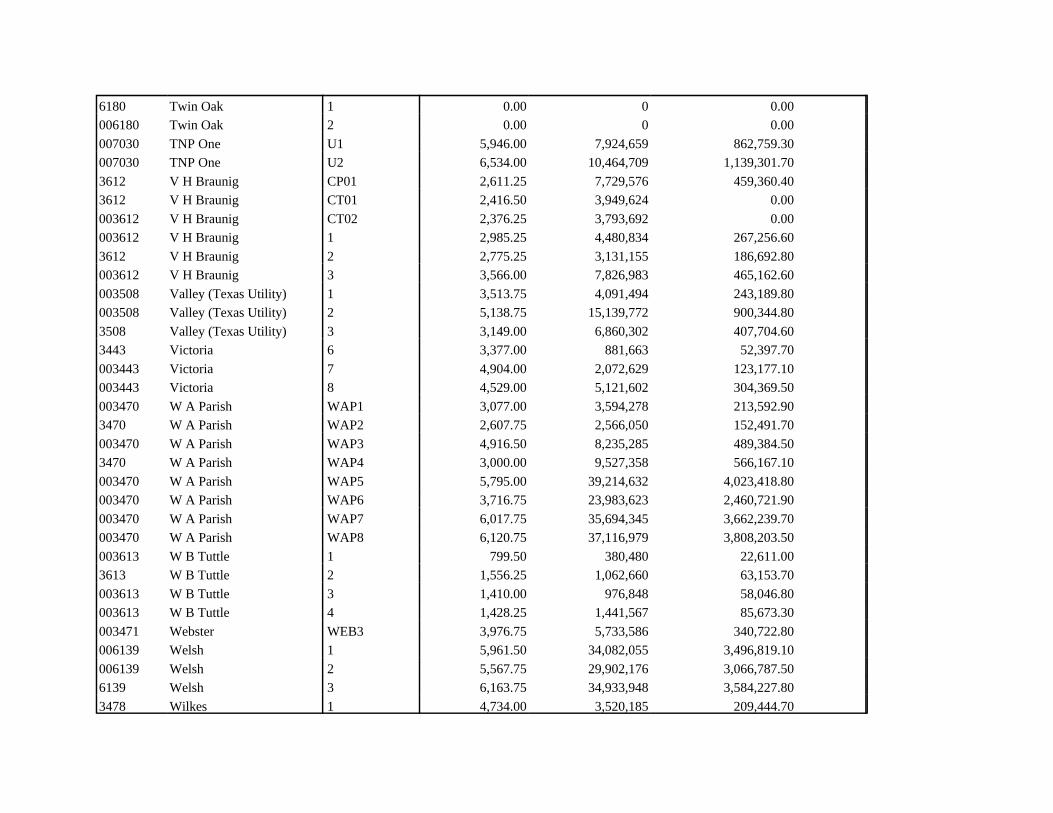
6180 Twin Oak 1 0.00 0 0.00006180 Twin Oak 2 0.00 0 0.00007030 TNP One U1 5,946.00 7,924,659 862,759.30007030 TNP One U2 6,534.00 10,464,709 1,139,301.703612 V H Braunig CP01 2,611.25 7,729,576 459,360.403612 V H Braunig CT01 2,416.50 3,949,624 0.00003612 V H Braunig CT02 2,376.25 3,793,692 0.00003612 V H Braunig 1 2,985.25 4,480,834 267,256.603612 V H Braunig 2 2,775.25 3,131,155 186,692.80003612 V H Braunig 3 3,566.00 7,826,983 465,162.60003508 Valley (Texas Utility) 1 3,513.75 4,091,494 243,189.80003508 Valley (Texas Utility) 2 5,138.75 15,139,772 900,344.803508 Valley (Texas Utility) 3 3,149.00 6,860,302 407,704.603443 Victoria 6 3,377.00 881,663 52,397.70003443 Victoria 7 4,904.00 2,072,629 123,177.10003443 Victoria 8 4,529.00 5,121,602 304,369.50003470 W A Parish WAP1 3,077.00 3,594,278 213,592.903470 W A Parish WAP2 2,607.75 2,566,050 152,491.70003470 W A Parish WAP3 4,916.50 8,235,285 489,384.503470 W A Parish WAP4 3,000.00 9,527,358 566,167.10003470 W A Parish WAP5 5,795.00 39,214,632 4,023,418.80003470 W A Parish WAP6 3,716.75 23,983,623 2,460,721.90003470 W A Parish WAP7 6,017.75 35,694,345 3,662,239.70003470 W A Parish WAP8 6,120.75 37,116,979 3,808,203.50003613 W B Tuttle 1 799.50 380,480 22,611.003613 W B Tuttle 2 1,556.25 1,062,660 63,153.70003613 W B Tuttle 3 1,410.00 976,848 58,046.80003613 W B Tuttle 4 1,428.25 1,441,567 85,673.30003471 Webster WEB3 3,976.75 5,733,586 340,722.80006139 Welsh 1 5,961.50 34,082,055 3,496,819.10006139 Welsh 2 5,567.75 29,902,176 3,066,787.506139 Welsh 3 6,163.75 34,933,948 3,584,227.803478 Wilkes 1 4,734.00 3,520,185 209,444.70

3478 Wilkes 2 4,828.00 9,289,209 552,043.303478 Wilkes 3 4,187.00 7,893,091 469,075.30

State Totals 991,836.00 2,295,468,863 184,470,007.40

B - 1

Appendix B. Programs for Reduction in Greenhouse Gases

There are several federal programs for the reduction of greenhouse gas emissions. Texascompanies figure in these statistics. However, the data was at a national level and it was notpossible to retrieve “Texas only” reductions from these tables. As the programs have indicatedprogress towards reductions, these programs are summarized here.

In 1999, EPA and DOE worked together toward a goal of doubling U.S. Combined Heatand Power (CHP) capacity by 2010 (an increase of 50 gigawatts). Since CHP uses significantlyless fuel than traditional power generation, it is estimated that the doubling of capacity will resultin 30 MMTCE in annual greenhouse gas emissions reductions and will reduce NOx emissions byhundreds of thousands of tons.

The Methane Partnership Program is made up of three separate programs: the LandfillMethane Outreach Program, Natural Gas STAR, and the Coalbed Methane Outreach Program. Methane is the most common non-CO2 greenhouse gas and it is 21 times more potent thancarbon dioxide. However, if captured, it can be used as a source of energy. It is the goal of theMethane Partnership Program to help U.S. industries and state and local governments reducemethane emissions. The estimate is that these programs, along with a regulatory program to limitlandfill emissions, will enable the U.S. to maintain methane emissions at or below 1990 levelsthrough 2010.1

The Coalbed Methane Outreach Program (CMOP), the last of the Methane Partnershipprograms, has as its goal the reduction of methane emissions from underground coal mines bytrapping the gas and using it for energy. The EPA estimates that its Partners increased thequantity of methane recovered to nearly 18 billion cubic feet or 2.0 MMTCE, which is equivalentto eliminating the emissions from about 1.5 million cars per year.2 While Texas is not listed as aPartner in the Coalbed Methane Outreach Program, a Texas company, BCCK Engineering ofMidland, Texas, is cited as having developed a cryogenic gas processing unit to upgrademedium-quality gob gas which was installed by Jim Walter Resources, a CMM Partner, at its #4,#5, and #7 Blue Creek mines in Alabama (see.http://www.epa.gov/coalbed/whatsnew.htm#p3. EPA estimates that the CMOP Partners wereresponsible for reductions of methane emissions amounting to 2.0 MMTCE in 1999.3

There are two Agriculture-Based Programs: AgSTAR and the Ruminant LivestockEfficiency Program. The focus of AgSTAR is to encourage the use of methane recovery (biogas)technologies at confined animal feeding operations that manage manure as liquids or slurries (seehttp://www.epa.gov/agstar/). The Ruminant Livestock Efficiency Program’s goal is to reducegreenhouse gas emissions from livestock production through management strategies that improveproduction efficiency and result in lower emissions per unit of milk or meat produced (seehttp://www.epa.gov/rlep/).

There are six separate programs in the EPA’s Environmental Stewardship Partnership. The reductions by Program are shown in Table B-1.

B - 2

Table B-1. Environmental Stewardship Partnerships

Program 1999 Emissions Reductions 4

The Voluntary Aluminum Industrial Partnership(VAIP)

PFC emissions–2.4 MMTCE

HFC-23 Emission Reduction Program HFC-23 emissions–2.7 MMTCE

The PFC Emission Reduction Partnership for theSemiconductor Industry

Goal: The reduction of PFC emissions to 10percent below 1995 levels by 2010

SF6 Emission Reduction Partnership for ElectricPower Systems

57 Partners worked during 1999 to establish baseline levels. There are six Texas companiesthat are Partners:

El Paso Electric Co., El Paso, TexasReliant Energy–HL &P, Houston, TexasSan Antonio City Public Service Board, San Antonio,TexasTexas Municipal Power Agency, Bryan, TexasTexas Utilities Electric Co., Dallas, TexasWest Texas Utilities, Abilene, Texas

SF6 Emission Reduction Partnership for theMagnesium Industry

Partners worked during 1999 to establish baseline levels

Society of Automotive Engineers Mobile AirConditioning Climate Protection Partnership

Goal: Promote cost-effective designs andimproved service procedures to minimizeemissions from HFC-134a refrigerants, whichreplace CFC-12 refrigerants

Local Government & Community Programs and Incentives for Renewable Energy 5

Austin ProgramsCOMMUNITY INVESTMENT & AWARENESSGreen PricingAustin Energy – GreenChoice

Among the most ambitious utility green pricing efforts to date, Austin Energy kicked off thenew millennium by inviting its 350,000 customers to sign up for GreenChoice. Under theGreenChoice program, residential and business customers may opt to apply the fuel chargeportion of their electric bill, plus a small premium, to obtain clean renewable energy. Inaddition, Austin Energy will match participants’ subscriptions dollar-for-dollar. Just 10months after officially launching its GreenChoice green pricing option, Austin Energy fully

B - 3

subscribed the initial 40 MW of wind and landfill-gas-generated electricity it will distributethrough its system beginning in 2001. In total, more than 3,000 customers have signed up forthe service. Unlike many other utility green pricing programs, business customers havecommitted to purchase a majority of the available power—nearly 85%.In October 2000, the Austin City Council decided to expand Austin Energy’s GreenChoiceprogram by 56.7 MW through the purchase of additional wind energy. The utility will nowsupply nearly 100MW of new renewables to its customers with most of the energy comingfrom wind. The action allows Austin Energy to purchase up to $8 million of wind power ayear over the 10-year term of the agreement. Through the expanded wind power purchase,Austin Energy expects to meet 53% of its projected load growth between 2000-2003 throughnew renewable energy sources and savings from energy efficiency. Other renewables beingdeveloped for the program include landfill gas recovery projects located in Austin, Houston,San Antonio and near Dallas.

Green Pricing/Renewable Energy ProjectsAustin Energy - Solar Explorer

Solar Explorer is a green pricing program created by Austin Energy to support photovoltaic (PV)installations on community facilities around Austin. All of Austin Energy’s customers areeligible to participate in Solar Explorer. The program officially got off the ground in 1998and is expected to operate for six years.Approximately 1252 blocks of solar power have been sold to almost 1000 residents andbusinesses who pay a monthly premium of $3.50 per 50-watt block and make a two-yearcustomer commitment. So far, these contributions have gone towards the construction ofthree grid-connected PV systems. One PV unit is located over the taxi waiting area atAustin’s Bergstrom Airport, the second system is on covered parking at the Howson branch ofthe Austin Library, while the third is also at the Airport. Austin Energy and a Solar ElectricPower Association (formerly UPVG) TEAM-UP grant cover the rest of the program’sfunding.Solar Explorer was promoted to the public through bill inserts and direct mailings toenvironmental organizations. Participants receive several promotional perks when they signup. These include a Solar Explorer membership card, a Solar Explorer T-shirt (first 640members only), and a Solar Explorer decal for home, business, or vehicle.

FINANCIAL INCENTIVESLoan & Rebate ProgramsAustin Energy – Home Energy Loans & Air Conditioning and Appliance RebatesAustin Energy began the Home Energy Loan program in 1985 as a program that offered low-interest financing to customers to finance home energy efficiency Customers choose one oftwo loan options: < 5.99%interest Home Improvement Loan – 3, 5, 7, or 10 year repayment periods, and

$6,000 maximum loan amount ($9,000 for duplexes); or < 7.99% interest Major Home Improvement Loan – 3, 5, 7, or 10 year repayment periods,

and $9,000 maximum loan amount.

B - 4

The Home Energy Air Conditioning and Appliance Rebate program offers customers a rebateon solar water heaters and energy-efficient equipment, such as heat pump water heaters, heatrecovery water heaters, and package air conditioners and heat pumps. Funding for the rebatescomes from Austin Energy’s revenues.For solar water heaters, there are three rebate options available to customers:< 16 square foot collector area or less – $150;< 16 to 35 square foot collector area – $250; and< 36 square foot collector area or more – $350.

Austin Energy promotes both the Home Energy Loan and the Home Energy Air Conditioningand Appliance Rebates programs to the public through bill inserts, on billboards, and inadvertisements for TV, newspapers, and magazines. The utility also publicizes the loans andrebates at presentations to neighborhood associations and businesses, and in literaturedistributed at home improvement shows and the Austin City Chamber of Commerce.Participating customers must choose to accept either the loan or the rebate, but not both.

State of Texas – Financial IncentivesProperty tax exemption – Solar and wind systems do not add to assessed property value for taxpurposes.Corporate deduction – Corporations can deduct 100% of the cost of a solar energy system from thestate franchise tax.Manufacturer incentive – Texas exempts solar manufacturers from the state franchise tax. Visitwww.ncsc.ncsu.edu/dsire.htm for more info on Texas’s incentives.

RULES, REGULATIONS & POLICIESNet Metering & Interconnection

Austin Energy will allow customer meters to run forward and backward. Beforeinterconnection can take place, Austin Energy must review the project specifications. PVsystems must be in compliance with the National Electrical Code and IEEE 929. As the laststep before interconnection, Austin Energy performs an inspection of the system and performsan anti-islanding test.

State of Texas – Regulatory PoliciesRenewable portfolio standard – 2880 MW of renewables must be installed by 2008; interim mark is1,280 MW by 2003.Net metering – All renewable technologies up to 50 kW are eligible for net metering. All customerclasses can net meter.State building requirements – state agencies must compare the cost of providing energy to newbuildings from alternative energy sources.Equipment certification – To be eligible for sales tax exemptions, solar collectors must be certifiedby the Solar Rating & Certification Corporation or the Air Conditioning & Refrigeration Institute.Disclosure – Retail energy providers must disclose information on fuel mix, environmental impacts,water consumed in producing power.Line extension – Electric utilities must provide information on renewable energy alternatives tocustomers requesting a line extension.Visit www.ncsc.ncsu.edu/dsire.htm for more info on Texas’s incentives.

B - 5

a

San Antonio Programs

COMMUNITY INVESTMENT & AWARENESSEducation & Assistance

Solar San Antonio, Inc.

Solar San Antonio is a nonprofit advocacy group sponsored by City Public Service, SanAntonio’s municipal utility. Initiated in July of 1999, Solar San Antonio is working with avariety of stakeholders to educate citizens and local governments in an effort to advancesustainable and renewable energy technologies. Here’s a look at some of their activities:

< Organized a regional alternative energy symposium in San Antonio on February 25th,2000. Itfeatured recognized experts in the field of renewable energy and drew 130 citizens, civicleaders,and guests;

< Held a Green Building symposium on September 22, 2000 for architects, builders,developers and government officials. The Symposium was sponsored by the U.S.Department of Housing and Urban Development, the City of San Antonio, Bexar County,San Antonio City Public Service and ICF Counseling;

< Held a charette to propose designs incorporating green building and renewable energytechnologies for one new building and one retrofit project for the City of San Antonio;

< Worked with a local community college to develop a training course for solar installers.There is currently no state solar contractor license requirement;

< Organized a seminar for local builders and bankers to educate them about a new FannieMae and Freddie Mac lending policy for energy efficient homes. The seminar was co-sponsored by Fannie Mae and Freddie Mac; and

< Worked with the City’s housing agency to incorporate solar hot water systems into itsnew 25-home construction project.

Renewable Energy Projects

City Public Service – Solar Customer Service Center

CPS is in the process of retrofitting a building to house its new customer service center -- onethat will be a showcase for renewable and energy efficient technologies. It will be aptlynamed “Solar Serve.” The nearly $7 million plan calls for PV and water-heating solar panels,natural gas air conditioners, and other green building elements. Solar Serve is being designedfor tours; equipment will be on display and available for hands-on inspection.

Parade of Affordable Homes

B - 6

CPS is providing funding to install solar hot water systems on 15 homes for next year’s“Parade of Affordable Homes.”

Green PricingSan Antonio City Public Service - Windtricity™ Program

City Public Service (CPS), serving more than 550,000 customers in San Antonio, beganoffering a wind power green pricing option to all of the city’s retail customers in April 2000.Power for the Windtricity™ program will eventually be supplied from a 25-MW wind projectplanned for West Texas. In the meantime, CPS is purchasing 600,000 kWh of wind powereach month from an existing wind project. Wind energy is available in 100-kWh blocks foran additional $4.00 per month, or a premium of 4¢/kWh. Customers can choose the numberof “blocks” they want, up to the total of their monthly electric use. There is no minimum timecommitment.

Participants receive a semi-annual newsletter relating to renewable energy and theenvironment, a Windtricity™ yard sign indicating that their home uses wind energy, and aWindtricity™ “window cling” for their vehicle.

State Programs

State Energy Conservation Office (SECO) Overview

Created in response to the Arab oil embargo of 1973 and the resulting national energycrisis, the Texas "energy office" has evolved from its original function of responding to state fuelshortage emergencies and administering federal energy conservation grants to its current role as astatewide promoter of energy efficiency and provider of energy management services which havea positive impact on state energy expenditures and local property tax rates.

Beneficiaries of SECO's services include: state agencies public schools city and county governments institutions of higher education private industries residential energy consumers

Originally known as the Governor's Energy Advisory Council (1975), the State EnergyConservation Office has been housed in a number of state agencies and undergone severalname changes. In 1999, the 76th Texas Legislature transferred the energy office to the TexasComptroller of Public Accounts.

The primary funding source for SECO programs has been oil overcharge settlement

B - 7

dollars resulting from federal court settlements of alleged violations of price controls in effect forcrude oil and refined petroleum products between 1973 and 1981. While the U. S. Departmentof Energy is the federal agency responsible for ensuring compliance with the court settlements,the state's responsibility is to return these funds to the citizens of Texas through promoting andsupporting energy efficiency and renewable energy programs according to state and federalguidelines.

SECO's task is to enable Texans to enjoy the optimal benefit from the domestic energywe produce, to contribute to our state's growing economy through reducing a major operationalcost of state government, school districts, municipal governments, hospitals, and smallbusinesses, to promote those technologies and procedures which result in cost effectiveoperation, and to show individual Texas residents how an energy efficient ethic can enhancetheir quality of life and that of future Texans.

Some of the programs overseen by or in which SECO participates include:Alternative FuelsBuilding Efficient TechnologiesClean CitiesCodes and StandardsColonias: Housing, Telehealth, Transportation, and Water PurificationHousing Energy EfficiencyHousing PartnershipHousing Trust FundInfinite PowerLoanSTARPerformance ContractingPhotovoltaicsRebuild TexasRenewable EnergyState Agency Energy Advisory GroupSchools/Local Government PartnershipsEnergy Manager TrainingEnergy Education OutreachTexas Energy Education DevelopmentWatt WatchersState Agencies ProgramSustainable Buildings DesignSustainable Schools Design Demonstration Project

(See http://www.seco.cpa.state.tx.us/)

B - 8

Texas General Land Office (GLO)

Texas Energy for a New Century:The GLO's Sustainable Energy Strategy is built on action items identified in the 1995

Texas Sustainable Energy Development Council strategic plan. The GLO leads the effort tomaximize the efficient use of Texas energy resources by developing and promoting sustainableenergy resources.

The strategy seeks to: identify opportunities for sustainable energy development on statelands, and educate citizens about opportunities for sustainable energy production on state landsthrough a statewide marketing plan.

The Texas Wind Power Project:The GLO, in partnership with the Lower Colorado River Authority and private

contractors, created one of the nation's largest wind power plants in the windswept DelawareMountains of far West Texas. (see http://www.glo.state.tx.us/sustain/#wind).

Lease payments from the project help support the state's Permanent School Fund (PSF).The project will ultimately pay more than $3 million to the PSF for the schoolchildren of Texas.

Greenbuilding Energy-Efficient Loans:The Greenbuilding Program of the GLO and the Texas Veterans Land Board (VLB) is the

nation's first loan program of its kind.

Eligible Texas veterans can take advantage of incentives that range from lower mortgagerates for energy-efficient new homes to home improvement loans for upgrading the efficiencyrating of an existing home.

Endnotes - Appendix C.

1. U.S. Environmental Protection Agency, Climate Protection Division, The Power to Make aDifference, ENERGY STAR and Other Partnership Programs, 1999 Annual Report, EPA 430-R-00-006, July 2000, pg 20

2. Ibid., pg 25

3. Ibid., pg 26

4. Ibid., pgs 28, 29

5. Susan Gouchoe, Local Government and Community Programs and Incentives for RenewableEnergy-National Report, North Carolina Solar Center, Industrial Extension Service, NorthCarolina State University, Raleigh, NC, December 2000, pgs 128-133

1 There is not a direct overlap in the facility populations of our utility sector and E-GRID’s power generators. E-GRID contains information on many non-utility power generators and cogeneration facilities that would not beincluded in the utility sector. See the Fossil Fuel Combustion Results section for more details.

Page 1

Appendix C. Methodology for Estimating Texas Greenhouse Gases

This chapter outlines the approaches used by ICF to estimate greenhouse gas emissions and sinksfor the 11 sources identified in the Texas Inventory. ICF followed the format of the Inventory of USGreenhouse Gas Emissions and Sinks, explaining the calculation methodology (i.e., what steps and dataare involved in the calculation), the data sources, and the uncertainty associated with each source’semissions estimates.

Fossil Fuel Combustion Carbon Dioxide (CO2)

Methodology

In estimating CO2 emissions from fossil fuel combustion in Texas, ICF followed an approachrecommended by the EIIP Workbook. This fuel- and sector-specific approach is based upon the methodsemployed by the Inventory of U.S. Greenhouse Gas Emissions and Sinks: 1990-1999 (EPA 2001) and fromthe Revised 1996 IPCC Guidelines for National Greenhouse Gas Inventories (IPCC 1997). The calculationrequires five steps:

1) Determine annual fuel consumption by fuel type and sector. The fuel type (e.g., coal, petroleum, naturalgas) and consumption sector (e.g., residential, commercial, industrial) are the primary activity data usedin the emissions calculations.

2) Estimate the total carbon content of each fuel consumed. Within each sector, each fuel’s consumptionis multiplied by a fuel-specific carbon content value to estimate the total amount of carbon consumed.

3) Estimate the amount of carbon stored in products. A portion of fuel consumption is used for non-energyend uses, i.e., the fuels are transformed into products such as asphalt, plastics, rubber, fibers, orlubricants, rather than combusted for energy. Since state-level data on non-energy fuel consumption isnot available, ICF apportioned the carbon contents of the fuels consumed into non-energy and energyend uses, within either the industrial or transportation sector. The split was made according to thepercentage of national sectoral fuel consumption designated for non-energy end uses for each year from1990-1999. The percentages for each fuel are shown in Table 2.1. The carbon consumed for non-energyend uses is then multiplied by a storage factor, which expresses how much non-energy carbon consumedis ultimately stored.

4) Estimate the total carbon potentially emitted. Total potential emissions are equal to the total carboncontent of the fuels consumed minus the amount of carbon stored in products.

5) Estimate the carbon actually oxidized during combustion. Due to inefficiencies in combustionprocesses, not all of the carbon combusted is oxidized into carbon dioxide; some remains behind as soot,ash, or other by-products. Oxidation efficiency is assumed to be 99 percent for the carbon in petroleumand coal fuels, and 99.5 percent for the carbon in natural gas.

6) Compare emissions estimates to CO2 emissions found in E-GRID. The Emissions and GenerationResource Integrated Database (E-GRID) is an electronic database maintained by the Clean Air MarketsDivision of the EPA that contains estimates on CO2 emissions for virtually every power plant andcompany that generates electricity in the United States. E-GRID provides emissions estimates for 1996,1997, and 1998. ICF compares the estimates of total combustion emissions and utility sector emissionsas a way to verify the methods.1

Table 2.1: Non-Energy Storage Factors and 1990 Non-Energy Fuel Consumption as aPercentage of Total Fuel Consumption

Fuel Sector and Type Storage Factor N o n - E n e r g yConsumption

Industrial

Asphalt and Road Oil 100% 100%Distillate Fuel 50% 1%Feedstocks, Naphtha 91% 100%Feedstocks, Other Oils 91% 100%LPG 91% 75%Lubricants 9% 100%Misc. Petro Products 100% 100%Natural Gas 91% 4%Pentanes Plus 91% 33%Petroleum Coke 50% 26%Residual Fuel 50% 11%Special Naphthas 0% 100%Waxes 100% 100%Transportation

Lubricants 50% 100%

Data Sources

Data on fuel consumption was taken from the State Energy Data Report, 1999 (EIA 2001) publishedby the Energy Information Administration (EIA) of the Department of Energy (DOE). The Report providesfuel consumption data organized by fuel type and consumption sector for each of the 50 states for 1960through 1999. The carbon content values were taken from the EIIP Workbook (EIIP 1999). Carbon storagefactors for non-energy end uses and oxidation efficiency values were found in the Inventory of U.S.Greenhouse Gas Emissions and Sinks: 1990-1999 (EPA 2001). The national sectoral fuel consumption andnon-energy fuel consumption data for 1990-1999, which is used to estimate Texas’s non-energy fuelconsumption, was also collected from the Inventory (EPA 2001). E-GRID emissions estimates were obtainedfrom the EPA’s Acid Rain Program website (http://www.epa.gov/airmarkets/egrid/index.html).

Uncertainty

The uncertainty associated with estimating CO2 emissions for fossil fuel combustion is generally low.The U.S. Inventory (EPA 2001) asserts that its emission estimates are accurate within 1 or 2 percent, withthe relatively low uncertainty attributable to the fact that fuel consumption (to which CO2 emissions areclosely linked) is carefully measured. Similarly, the measured CO2 emission estimates for utilities (from E-GRID) are based on continuous emission monitoring (CEM) that must meet performance standards. Thus,these estimates also carry relatively low uncertainty.

Probably the greatest uncertainty in our calculations arises from the estimate of carbon stored vianon-energy uses of fossil fuels. The non-energy fuel consumption values for 1990 through 1999 areestimated by applying the percentage of national non-energy fuel consumption to a sector’s total fuelconsumption. Using the percentages to apportion the data assumes that the proportion of fuel used fornon-energy end uses in Texas is similar to the proportion for the country as a whole. Also, the storagefactors are assumed values, reported originally by Marland and Rotty (1984) and updated in a recent draftEPA analysis. They are not based on actual product production or fuel consumption data.

To a lesser extent, uncertainties arise from the carbon content values and the oxidationefficiencies. The carbon contents may vary within a fuel type and the oxidation efficiencies may vary bycombustion location; however, these variations are considered very small.

Overall, there is considerably less uncertainty surrounding the estimate of CO2 from fossil fuelcombustion than for any of the other sources covered in the inventory.

Coal Mining Methane Emissions

Methodology

In estimating Texas CH4 emissions from surface coal mining, ICF followed the approachrecommended by the EIIP Workbook. Emissions are the sum of (1) emissions that occur during surfacemining and (2) post-mining emissions. The calculation requires the following steps:

Emissions from Surface Mining Activity

1) Determine the annual surface mine production in Texas. Coal production from surface mines inmetric tons is the primary activity data used in the emissions calculations.

2) Multiply production data by the specific surface mining emissions factor to obtain emissions. Theemission factor of 6.4 ft3 CH4/short ton coal (EIIP 1999) is a coal basin-specific estimate andaccounts for methane liberated from the coal itself as well as the surrounding strata. The followingformula was used to estimate methane emissions from this sub-sector:

Emissions from surface mines (ft3 CH4) = Surface Coal Production (short tons) x 6.4 (ft3

CH4/short ton).

Emissions from Post Mining Activity

3) Multiply production data by the specific post-mining emissions factor to obtain emissions. Theemission factor of 1.04 ft3 CH4/short ton coal (EIIP 1999) is a basin-specific estimate and thefollowing formula was used to estimate methane emissions from this sub-sector:

Emissions from post-mining operations (ft3 CH4) = Surface Coal Production (short tons) x 1.04(ft3 CH4/short ton).

Total Emissions from Surface Mining Activity

4) Estimate total emissions from coal mining operations. Total emissions for coal mining activities inTexas are equal to the aggregate sum of emissions from surface mining and post-mining activities.

Data Sources

Data on coal production from surface mines in Texas were collected from the EnergyInformation Administration’s Coal Industry Annual of the Department of Energy (DOE). Emissionfactors for surface and post-mining operations were taken from the EIIP Guidance and the U.S. Inventory(EIIP 1999, EPA 2001).

Uncertainty

A high level of uncertainty is associated with methane emissions from surface-mining operationsas emissions may be from one to three times more than the in-situ methane content of coal (EIIP, 1999). EIIP also states that available information indicates that coal mined from surface mines contains lowamounts of methane. Other factors such as coal seam quality and moisture also affect emissions.

The US Inventory (EPA 2001) also states that there is also considerable difficulty in estimatingaccurate emissions factors. There are no specific emissions factors for Texas; rather emissions factorsused for activity in Texas are also applied to a number of other states.

According to EIIP, the uncertainty in surface-mining and post-mining emissions estimates is ±50percent.

2 Associated wells produce both gas and oil; non-associated wells produce only gas.

Page 4

Petroleum Systems Methane Emissions (CH4)

Methodology

The petroleum system is characterized by three major stages: field production, transportation, andrefining. Methane emissions from petroleum systems generally stem from fugitive emissions, ventedemissions, fuel combustion emissions, and from operational upsets (EPA, 2001). Methane emissionsfrom petroleum systems were estimated using the methodology described in EIIP Volume VIII,Estimating Greenhouse Gas Emissions (1999). The calculation requires two steps:

1) Obtain activity data. Oil production and the amount of oil and natural gas vented/flared are theprimary activity data used in the emissions calculations. Activity data associated with thetransportation and refining stages of petroleum systems were not available.

2) Estimate Methane Emissions. Methane emission estimates were calculated by multiplying the activitydata by the corresponding emission factor. Emission factors were obtained from the EIIP Workbook.

Data Sources

Oil production data for 1990 through 1999 were collected from the Energy InformationAdministration (EIA) (EIA 2001a). Oil production data for 2000 was obtained from the Railroad Commissionof Texas, Oil & Gas Division (RCTX 2001). Oil and Gas Vented/Flared data was obtained from EIA’sHistorical Natural Gas Annual: 1967 through 1999 (EIA 2001b). 2000 data was obtained from the RailroadCommission of Texas, Oil & Gas Division (RCTX 2001). Emission factors were taken from the EIIPWorkbook (EIIP 1999).

Uncertainty

There is uncertainty associated with the estimate of annual venting emissions in production fieldoperations. The majority of methane emissions occur during these operations, where methane can firstescape from crude oil. However, there is a limited understanding of tanks, tank equipment, and vaporrecovery practices that are associated with these emissions (EPA 2001). There is also uncertaintyassociated with the emission factors used to estimate emissions. This uncertainty arises from the fact thatemission rates can vary widely from reservoir to reservoir and well to well. A single average emissionfactor cannot reflect this variation.

Natural Gas Systems Methane Emissions (CH4)

Methodology

The natural gas system is characterized by four major stages: field production, processing,transmission and storage, and distribution. Methane emissions from natural gas systems are associated withnormal operations, system upsets, and routine maintenance associated with each of the four stages of thenatural gas system (EPA 2001). In estimating Texas’s CH4 emissions from natural gas systems, ICF followedan approach recommended by the EIIP Workbook (EIIP 1999) by basing emissions on a set of activity levelsfor the activities from which methane is emitted. The calculation requires five steps:

1) Obtain activity data for the production sector. For estimating natural gas production emissions, datarelating to the total number of non-associated and associated2 wells and the miles of gathering pipelinewere collected. Since state-level data was unavailable for associated wells, ICF assumed that they

comprise of 46% of the total number of oil wells. This ratio is based on assumptions employed by theInventory of US Greenhouse Gas Emissions and Sinks: 1990-1999 (EPA 2001). Due to the lack of data,the number of miles of gathering pipeline for 2000 was used for the entire time series. The EIIPWorkbook also suggests including emissions associated to the number of offshore platforms in the Gulfof Mexico, but these data were not available.

2) Obtain activity data for the processing sector. For estimating natural gas processing emissions, ICFobtained data on the number of gas processing plants. Data on gas processing plants was unavailable for1990 through 1995. For this period, the number of processing plants was estimated by extrapolating data,assuming a least-squares fit, from the period 1996 through 2000.

3) Obtain activity data for the transmission sector. For estimating natural gas transmission emissions, ICFobtained data on miles of transmission pipeline and number of transmission and storage stations. Dueto a lack of data, the number of transmission pipeline miles for 2000 was kept constant for the entire timeseries. Similarly, the 1998 transmission and storage stations number was kept constant for the wholetime series. The EIIP Workbook also suggests including emissions associated with the number of LNGstations, but these data were unavailable.

4) Obtain activity data for the distribution sector. For estimating natural gas distribution emissions, thenumber of miles of cast iron, steel and plastic distribution mains pipeline was obtained. Miles of steeldistribution pipeline was broken into unprotected steel and protected steel by allocating 85% of totalsteel to protected steel and 15% to unprotected steel. This ratio is based on assumptions employed bythe Inventory of US Greenhouse Gas Emissions and Sinks: 1990-1999 (EPA 2001). Activity data for theperiod 1990 through 1993 in the distribution sector was unavailable. Estimates for this period wereobtained by extrapolating data from 1993-2000. The EIIP Workbook also suggests including emissionsassociated to the number of services (unprotected and protected), but these data were unavailable.

5) Estimate Methane Emissions. To estimate methane emissions ICF multiplied the activity data by theircorresponding emission factors. Emission factors were obtained from the EIIP Workbook.

Data Sources

Data were collected using a number of sources. Data on the number of non-associated wells wastaken from the Energy Information Administration’s (EIA) Historical Natural Gas Annual (EIA 2000) andthe Railroad Commission of Texas, Oil & Gas Division (RCTX 2001). The total number of oil wells wasobtained from the EIA (EIA 2001a), and from the Railroad Commission of Texas, Oil & Gas Division(RCTX 2001). Data for miles of gathering pipeline was obtained from the Railroad Commission of Texas,Oil & Gas Division (RCTX 2001). The number of gas processing plants was taken from the Oil & GasJournal (O&GJ 1997, 1998, 1999, 2000, 2001). Data on the number of natural gas transmission and storagestations were obtained from the EIA, Office of Oil and Gas, Reserves and Natural Gas Division'sGeographical Information System- Natural Gas CD (EIA 1998). Data on the miles of transmission pipelinewas obtained from the Railroad Commission of Texas, Oil & Gas Division (RCTX 2001). Data on miles ofcast iron, steel and plastic distribution pipelines were obtained from the Department of Transport (DOT),Office of Pipeline Safety (DOT 2001). Emission factors were taken from the EIIP Workbook (EIIP 1999).

Uncertainty

Emission factors associated with the natural gas industry are based on measurement studiesconducted at various facilities throughout the United States. Typically, highly variable emission rates weremeasured among many of the system components, making the calculated average emission rates uncertain.Also, the heterogeneous nature of the natural gas industry makes it difficult to sample facilities that arecompletely representative of the entire industry. Because of this, scaling up from model facilities introducesa degree of uncertainty. The Inventory of US Greenhouse Gas Emissions and Sinks: 1990-1999 estimatesuncertainties associated with emissions from this source to be on the order of ±40 percent (EPA 2001).

Landfills Methane Emissions

Methodology

Like the fossil fuel combustion CO2 emissions, ICF estimated methane (CH4) emissions from landfillsusing the method found in the EIIP Workbook (EIIP 1999). This method uses both state-level informationon annual waste disposal and landfill-level information about the size and methane-collecting capacity ofTexas’ landfills. Net methane emissions are equal to the amount of methane generated by landfills, less theamount of methane collected by flaring or utilization systems, and less the amount of methane oxidized bysoil. The steps to estimating these three factors are shown below:

1) Determine Texas’ Municipal Solid Waste (MSW) 30-year Waste-In-Place (WIP). Waste has a methanegenerating capacity for approximately 30 years following disposal. The amount of waste discarded toTexas landfills in the previous 30 years, or the 30-year WIP, was estimated by adding historical seriesof annual waste disposal-to-landfill data.

2) Apportion the MSW 30-year WIP into large or small landfills. Since large landfills (greater than 1.1million metric tons of WIP) exhibit different methane emissions patterns than small landfills, the 30-yearWIP must be apportioned accordingly. The percentage of total Texas WIP residing in large landfills in1999 was estimated from individual landfill data. This percentage was used to split Texas 30-year WIPinto large and small landfills for 1990 through 1999.

3) Classify the large and small landfills as arid or non-arid. Landfills in arid regions (greater than 25inches of rain/year) produce less methane emissions than landfills in non-arid regions. Landfills wereclassified by the average annual precipitation of the cities or counties in which they reside.

4) Calculate methane generated from MSW. The following equations were used to estimate methanegeneration:

Methane generated at small non-arid landfills =(0.35 ft3 CH4/day) x (0.0077 (tons CH4/yr)/(ft3 CH4/day)) x (Total 30-year WIP at small landfills)

Methane generated at small arid landfills =(0.27 ft3 CH4/day) x (0.0077 (tons CH4/yr)/(ft3 CH4/day)) x (Total 30-year WIP at small landfills)

Methane generated at large non-arid landfills =Number of Large Landfills x (0.0077 (tons CH4/yr)/(ft3 CH4/day)) x

[417,957 tons CH4 + (0.26 ft3 CH4/day) x (total 30-year WIP at large landfills/Number of LargeLandfills)]

Methane generated at large arid landfills =Number of Large Landfills x (0.0077 (tons CH4/yr)/(ft3 CH4/day)) x

[417,957 tons CH4 + (0.16 ft3 CH4/day) x (total 30-year WIP at large landfills/Number of LargeLandfills)]

5) Calculate methane generated from industrial waste landfills. Since data on industrial landfill WIP wasunavailable for Texas, the methane generated from industrial landfills was assumed to equal 7 percentof the total methane generated by MSW landfills, consistent with the EIIP Workbook guidance (1999).

6) Determine the amount of methane flared or collected. ICF estimated the amount of methane collectedusing individual landfill data concerning the number and capacity of operating flares and landfill-gas-to-energy projects in Texas. For facilities that utilized flares for which specific efficiency data was notavailable, the amount of methane flared was estimated to be 75 percent of the total methane generated.

7) Correct for methane which is oxidized by soils. Approximately ten percent of the methane generated isoxidized by the soils surrounding a landfill. Thus, the total methane generated that is not flared orcollected is multiplied by 0.9 to yield the net emissions.

Data Sources

To calculate emissions using this method, two sets of data are necessary: a historical time series ofstate-level annual waste disposal data, and landfill-level information which characterizes the size, number,and CH4-flaring or -collecting capacity of the state’s individual landfills. The landfill information wasassembled from communications with TNRCC personnel. The equations for estimating methane generationat the small and large, arid and non-arid landfills, the factor for calculating emissions from industrial wastelandfills, and the factor for methane oxidation in soils are all found in the EIIP Workbook (1999). The flaringefficiency factor was taken from Greenhouse Gas Emissions from Management of Selected Materials inMunicipal Solid Waste (EPA 1998).

Uncertainties

The methane generation equations are the chief contributor to the overall method’s uncertainty. EPAcharacterizes the large landfill equation as having an uncertainty of ±15 percent while the small landfillequation, based on fewer actual field measurements, is accurate to ±20 percent. Another source ofuncertainty lies in the estimate of methane flared. Individual landfill flaring efficiency data was not available,as LMOP only provides a comprehensive profile of landfill-gas-to-energy projects. However, the uncertaintyassociated with this factor is significant; the assumed flaring efficiency is a “best estimate” based on a varietyof expert comments (EPA 1998). Lastly, the apportionment of Texas’ 30-year WIP was made using anincomplete list of large landfills, and ICF may have underestimated large landfill WIP by as much as 25percent. However, this factor’s contribution to uncertainty in the overall emissions is small. The total TexasWIP data was derived from a state survey, a source independent of landfill-level WIP data. Changes to theestimate for number of large landfills or large landfill WIP would only reallocate the total Texas 30-yearWIP used in our calculations. Even if additional large landfills were added to our database, the increase inemissions from the large landfills would be counterbalanced to some degree by a decrease in small landfillemissions, leading to small changes in net emissions.

Cement Manufacture Carbon Dioxide Emissions

Methodology

Carbon dioxide (CO2) is a by-product of a chemical conversion process used in the production ofclinker, which in turn is a component of cement. During this process, limestone (CaCO3) is heated tohigh temperatures in a kiln to form lime (Calcium Oxide or CaO). The simplified stoichiometricrelationships is as follows:

CaCO3 + heat → CaO + CO2

Estimates of Texas carbon dioxide emissions from cement production were based on thefollowing equation presented in EIIP Volume VIII: Estimating Greenhouse Gas Emissions (1999):

Texas CO2 Emission= (State Clinker Production x CaO Content(%) X 0.785) x CKD Correction factor

The quantity of clinker produced in Texas was multiplied by the percent lime (CaO) content ofthe clinker. The default CaO content is 65 percent (IPCC 2000). To obtain the total metric tons of CO2

emitted, ICF multiplied the quantity of CaO by its corresponding CO2/CaO stoichiometric ratio. TheCO2/CaO stoichiometric ratio: molecular weight of CO2 (44g)/molecular weight of CaO (56g) = 0.785.

CO2 emissions may also be emitted from cement kiln dust (CKD) that is not recycled to theproduction process. The CKD is largely a mix of calcinated and uncalcinated raw materials and clinker,and accounts for the portion of materials that does not become part of the clinker, and is lost to thesystem. To account for CO2 emissions emitted from cement kiln dust (CKD), IPCC recommends thatthese additional CKD CO2 emissions should be estimated as 2 percent of the CO2 emissions from clinkerproduction (IPCC 2000). Hence, ICF multiplied the total metric tons of CO2 emitted during clinkerproduction by the CKD correction factor of 1.02.

Data Sources

All data was taken from the USGS Annual Reports for Cement. The lime (CaO) content ofclinker as well as the default clinker kiln dust (CKD) correction factor were obtained from the IPCCGood Practice Guidance (IPCC 2000).

Uncertainty

Uncertainties in these estimates are primarily due to uncertainties in the lime content of clinker,in the amount of lime added to masonry cement, and in the percentage of CKD recycled inside the clinkerkiln. The lime content of clinker varies from 64 to 66 percent. CKD loss can range from 1.5 to 8 percentdepending on plant specifications. Additionally, some amount of CO2 is reabsorbed when the cement isused for construction. As cement reacts with water, alkaline substances such as calcium hydroxide areformed. During this curing process, these compounds may react with CO2 in the atmosphere to createcalcium carbonate. This reaction only occurs in roughly the outer 0.2 inches of surface area. Because theamount of CO2 reabsorbed is thought to be minimal, it was not estimated.

Adipic Acid Production Nitrous Oxide Emissions

Methodology

There are four Adipic acid plants in the United States, two of which are located in Texas. Nitrousoxide emissions from these plants were calculated by multiplying adipic acid production by the ratio ofN2O emitted per unit of adipic acid produced, and adjusting for the actual percentage of N2O released asa result of plant-specific emission controls. Because emissions of N2O are not regulated, emissions havenot been characterized well. However, on the basis of experiments, the overall reaction stoichiometry forN2O production in preparation of adipic acid was estimated at approximately 0.3 kg of N2O per kilogramof product. Emissions are determined using the following equation:

N2O emissions = [production of adipic acid] x [0.3 kg N2O / kg adipic acid] X [1 – (N2O destruction factor x abatement system utility factor)]

The “N2O destruction factor” represents the amount of N2O expressed as a percentage of N2Oemissions that are destroyed by the currently installed abatement technology. The “abatement systemutility factor” represents the percent of time that the abatement equipment operates. The destructionfactor is assumed to be 95 percent for catalytic abatement and 98 percent for thermal abatement. Theabatement system utility factor is assumed to be 95 percent for catalytic abatement and 98 percent forthermal abatement.

Data Sources

1990-1995 Data was originally reported in Chemical and Engineering News’ “Facts andFigures” and “production of Top 50 Chemicals”. Industry experts provided 1996 and 1997 productionvalues. 1998 data was reported in Chemical Week on March 10, 1999. Production was assumed to holdconstant in 1999 and 2000.

The emission factor was taken from Thiemens and Trogler (1991). The abatement system destructionfactor and utility factor were taken from Reimer et al. 1999.

Uncertainty

N2O emissions are controlled in some adipic acid production facilities, therefore the amount of N2Othat is actually released depends on the level of controls in place at specific production plants. Thus, in orderto calculate accurate emission estimates, it is necessary to have production data on a plant-specific basis. Inmost cases, however, these data are confidential. As a result, plant-specific production figures were estimatedby allocating total adipic acid production using existing plant capacities. This creates a degree of uncertaintyin the adipic acid production data used to derive the emission estimates as it is necessary to assume that allplants operate at equivalent utilization levels.

3 The description of methodology described in this section is summarized from the draft report CarbonStock Changes in Texas Forests, 1987-1997, by R.A. Birdsey and G.L. Lewis.

Page 10

The emission factor was based on experiments that attempt to replicate the industrial process and,thereby, measure the reaction stoichiometry for N2O production in the preparation of adipic acid. However,the extent to which the lab results are representative of actual industrial emission rates is not known.

Carbon Flux from Land Use Change and Forestry3

Methodology

Carbon sequestration and emissions associated with Land Use Change and Forestry are characterizedthrough the application of a U.S. Department of Agriculture, Forest Service (USDA-FS) model that tracksforest carbon flows related to tree growth, forest removals, and decomposition. The model partitionsecosystem carbon (C) into three separate components:

• biomass, which includes all aboveground and belowground portions of all live and deadtrees and understory vegetation

• forest floor, which includes all dead organic matter above the mineral soil horizons• Soil, which includes all organic C in the mineral horizons to a depth of 1 m.

The carbon estimates for the forest components are based on forest age, type,productivity class, and land use history. These parameters characterize the forest andecosystem carbon dynamics, as well as the understory, soil, and forest floor models that bestdescribe carbon flows. Additionally, the model tracks carbon in forest products (e.g., lumber,plywood, paper), accounting for the C sequestered during products’ lifetimes, as well as carbonstored (net of degradation) in landfills.

Estimates of carbon stocks are not made for each year; rather, they are simulated at five-yearintervals (1987, 1992, and 1997). For any year bracketed by these dates, the change in carbon stored overthe interval, divided by five years, is the annual flux. ICF extrapolated the values for 1997 to 1998 and 1999.

Data Sources

The forest carbon model is maintained by the USDA-FS and is detailed in the working paper entitled“Carbon Stock Changes in Texas Forests, 1987-1997.” The model draws on forest inventory data that is alsomaintained by USFS. The equations and models used to estimate carbon storage are documented throughoutthe literature. Birdsey (1996) provides details on forest carbon storage methods; Row and Phelps (1991) givethe foundation for quantifying carbon in forest products; and Birdsey and Schreuder (1993), Birdsey et al.(1993), and Birdsey (1996) explain the models used for estimating soil carbon.

Uncertainty

The largest contributor to the overall uncertainty lies in the estimate of the soil carbon. Themodels and data used to generate the soil carbon estimates are not usually part of a regional statisticalsample. Although the absolute uncertainty is difficult to quantify, the fact that the soil carbon constitutesover half of the overall carbon stock makes this an important source. Carbon flows in landfills (and to alesser extent, forest products) are also highly uncertain, due partly to the paucity of data on the fate ofharvested carbon, and partly to the assumption that Texas’ consumption and disposal of forest products isequal to the production from its forests.

In addition to the general uncertainty associated with the modeling of forest carbon, there aresome specific uncertainties associated with the Texas analysis as a result of reclassification of foresttypes and lack of consistent age class information. The data on which the estimates are based – forestsampling for 1987 and 1997 – are inconsistent for West Texas and East Texas. There are also some foresttype classification changes apparent in the data that may result from procedural differences rather thanactual changes in resource characteristics. Also, the data on West Texas address only changes in area ofvarious land use and forest categories, and therefore changes in biomass or other ecosystem carbon poolsdo not reflect increases or decreases in carbon stocks on land that did not change between forest and non-forest categories. Thus, these estimates in carbon stock changes should be used with extreme cautionuntil additional data for West Texas becomes available.

The estimates of above-ground biomass are the most certain of the component estimates. However, the regression models that convert the field measurement data into biomass carbon values aresubject to estimation errors.

The model itself accrues uncertainty since it does not account for all factorsaffecting forest carbon changes. Certain processes, such as the effect of atmosphericnitrogen deposition on soil and tree biomass carbon, have not been integrated into themodel’s calculations.

Enteric Fermentation Methane Emissions

Methodology

Like almost all the other sources, enteric fermentation emissions are estimated using the methodoutlined in the EIIP Workbook. Emissions are calculated for each animal type listed in Table 2.2, and areequal to the product of population and a methane generation factor. The methane generation factors (Table2.2) are region- and animal-specific, and are derived from EPA models that simulate animal production anddigestion. For Texas, ICF used the factors for animals in the South Central region.

Table 2.2: Methane Generation Factors for the South Central Region

Animal Type Methane Generation Factor(lbs CH4/head/year)

Dairy

Mature Cows 265.7Replacements 0-12 44.7Replacements 12-24 135.7Beef

Mature Cows 155.9Replacements 0-12 51.9Replacements 12-24 148.9Bulls 220.0Sheep 17.6Goats 11.0Swine 3.3Horses 39.6Mules/Asses 48.5

Data Sources

Data for non-equine animal populations was taken from the background documentation used inpreparing the Inventory of U.S. Greenhouse Gas Emissions and Sinks: 1990-1999 (EPA 2001). This datais organized at the state level and has been compiled from reports issued by the National AgriculturalStatistics Service (NASS) of the U.S. Department of Agriculture (USDA). An estimate for the equinepopulation for 1998 and 1999 was obtained from the Texas Agricultural Statistics Service (TASS 2001).

Horses were assumed to constitute the entire equine population, since their numbers overwhelm any of theother equine animal types. Emission factors were obtained from the EIIP Workbook (EIIP 1999).

Uncertainty

According to the Inventory, the method for estimating emissions from enteric fermentation isaccurate to ± 20 percent. The digestion model inputs used to determine the emissions factors draw from abroad representation of potential feeding strategies; differences between these inputs and actual practice inTexas introduce uncertainty. Due to sub-annual fluctuations in animal populations, uncertainty exists in allthe population statistics. Lastly, the assumption that horses are the only equine animals in Texas introducesuncertainty; however, the impact on the overall emissions estimate is small.

Manure Management Methane and Nitrous Oxide Emissions

Methodology

Methane and nitrous oxide (N2O) emissions from manure management systems are estimated usingthe methods outlined in the EIIP Workbook. Both types of emissions are functions of livestock populations,animal-specific emissions factors, and manure management system emissions factors. The steps forcalculating the CH4 and N2O emissions are outlined below:

1) Estimate Methane Emissions. The main driver of CH4 emissions is the quantity of volatile solidsproduced by livestock. Volatile solids are defined as the solid organic fraction of manure that willoxidize and be driven off as a gas at a temperature of 1,112°F. To estimate the amount of volatilesolids, ICF multiplied livestock population by a typical animal mass (TAM) factor and the volatilesolid/TAM ratio. The potential methane emissions are then calculated by multiplying the volatilesolids estimate by an animal-specific methane generating capacity factor. Finally, for each possiblemanagement system, the potential emissions were multiplied by a Methane Conversion Factor (MCF)that accounts for the affect a particular management system has on methane emissions. The MCF isalways between zero and one, with zero representing a zero emissions management practice andone representing a practice that maximizes methane emissions.

2) Estimate Nitrous Oxide Emissions. The main driver of N2O emissions is the amount of unvolatilizednitrogen in manure, either organically bound or in the form of ammonia. This quantity of nitrogen istermed the total Kjeldahl nitrogen. ICF estimated Kjeldahl nitrogen as the product of animal population,TAM, and the ratio of TAM to Kjeldahl nitrogen. Eighty percent of the total Kjeldahl nitrogen wasconsidered to remain unvolatilized. To calculate emissions, the unvolatilized nitrogen was multiplied bya management system emission factor that expresses how much of the nitrogen is emitted as N2O. Theemission factor for dry management systems (e.g., solid storage, drylot) is 2 percent of totalunvolatilized nitrogen; for liquid management systems the factor is 0.1 percent of total unvolatilizednitrogen. It is important to note that this method only calculates emissions for managed systems; N2Oemissions from manure applied to agricultural soils via daily spread operations or deposition ontopasture, range, or paddock are accounted for under the agricultural soils method.

Data Sources

Data for non-equine animal populations were taken from the background documentation used inpreparing the Inventory of U.S. Greenhouse Gas Emissions and Sinks: 1990-1999 (EPA 2001). This datais organized at the state level and has been compiled from reports issued by the National AgriculturalStatistics Service (NASS) of the U.S. Department of Agriculture (USDA). An estimate for the equinepopulation for 1998 and 1999 was obtained from the Texas Agricultural Statistics Service (TASS 2001).Horses were assumed to constitute the entire equine population, since their numbers overwhelm any of theother equine animal types. Methane and nitrous oxide emissions factors as well as the factors describingmanure management systems in Texas, animal TAM, volatile solid production, methane generating capacity,methane conversion, and Kjeldahl nitrogen content are all taken from the EIIP Workbook (EIIP 1999).

Uncertainty

The largest uncertainty in the CH4 emissions estimate is related to the MCFs. Very few fieldmeasurements are available upon which to base these conversions factors, particularly for dry managementsystems such as dry lots, pastures, and paddocks. However, the uncertainty in the CH4 estimate is lower thanthe uncertainty of the N2O estimate. The emission factors for N2O represent global averages, are based onlimited data, and are highly uncertain.

Agricultural Soils Nitrous Oxide Emissions

Methodology

The principal GHG from this sector is N2O; emissions are estimated using the method found inthe EIIP Workbook. There are two types of N2O emissions from soils: direct emissions, where the N2O isemitted from nitrogen-related cropping practices, and indirect emissions, where nitrogen-containingcompounds are released to the atmosphere or groundwater, and following denitrification/nitrification, areemitted as N2O. Sources of direct emissions include fertilizer and manure use in cropping, application ofcrop residues to soils, production of nitrogen-fixing crops, and cultivation of high-organic content soils(histosols). Histosol data was not available for Texas. Indirect emissions arise from fertilizer use,animal manure, and nitrogen-containing leachate and runoff.

To calculate both the direct and indirect emissions, ICF took the following 4 steps:

2) Determine the total nitrogen available for emission as N2O.

a) Estimate the amount of nitrogen in synthetic and organic fertilizers used annually. Data for thetotal nitrogen load of synthetic fertilizer is available at the state level, but it is provided for thegrowing season, from July 1 to June 30. To estimate the nitrogen used in synthetic fertilizerduring the calendar year, ICF assume that 65 percent of a given year’s fertilizer consumptiontakes place between January and June, while the remaining 35 percent occurs between July andDecember. Total organic fertilizer consumption data for the growing season is used to estimateannual organic fertilizer consumption in the same way as above. However, to avoid double-counting the emissions from manure (manure is handled in Step b), the organic fertilizerconsumption must be adjusted to represent only non-manure organic fertilizers. Since state-level data on the types of organic fertilizer consumed is not available, the percentage of regionalnon-manure organic fertilizer consumption for each year is used to apportion total organicfertilizer consumption. Lastly, non-manure organic fertilizer consumption was multiplied by itsaverage nitrogen content.

4 Kjeldahl nitrogen refers to amount of nitrogen that is either organically bound or in the form ofammonia. 5 Leachate and runoff, a source of indirect emissions, is a slightly different case. Emissions fromleachate and runoff are a function of the unvolatilized nitrogen that enters groundwater.

Page 14

b) Estimate the amount of nitrogen in manure. The nitrogen in manure was calculated for eachanimal type. It is equal to the product of the animal population, the typical animal mass (TAM), and theKjeldahl nitrogen emission factor.4

Amount of Nitrogen in Manure = Animal Population (head) x TAM (kg/head) x Kjeldahl nitrogenemission factor (kg N/1000 kg animal mass/day) x 365 days/year

c) Estimate the amount of nitrogen returned to soils from crop residues. Often, much of the cropmass is not harvested (e.g., the stalks and cobs of corn), but left on the field. Nitrogen fromresidues of corn, wheat, soybeans, and peanuts was estimated. The amount of nitrogen that theresidues add to soils is equal to the product of the crop production, the mass ratio of residue tocrop, the dry matter fraction of the crop residue, the amount of residue that is not burned, andthe nitrogen content of the residue.

Amount of Nitrogen Returned to Soils from Crop Residues = Crop Production (kg) x Ratio ofResidue Mass to Crop Mass (kg residue/kg crop) x Dry Matter Fraction of Residue (kg dm/kgresidue) x Percentage of Residue Not Burned x Nitrogen Content (kg N/kg dm)

d) Estimate the amount of nitrogen added to soils by nitrogen-fixing crops. The amount of nitrogenadded to soils by legumes was calculated as the product of legume production, the fraction ofdry matter, and the nitrogen content. The production mass was adjusted to include the residue.

Amount of Nitrogen Returned to Soils from Nitrogen-Fixing Crops = Crop Production (kg) x (1 +Ratio of Residue Mass to Crop Mass (kg residue/kg crop)) x Dry Matter Fraction of Residue (kgdm/kg residue) x Nitrogen Content (kg N/kg dm)

2) Classify the nitrogen as volatilized or unvolatilized. Direct emissions result from nitrogen that residesin soil being transformed into atmospheric N2O. Indirect N2O emissions, on the other hand, involvethe transport of nitrogen from the soil to another matrix (either the atmosphere or groundwater), andusually as a species other than N2O. Emission then takes place from this intermediate matrix. Generally, unvolatilized nitrogen is the source of direct emissions; volatilized nitrogen is the sourceof indirect emissions.5 One hundred percent of the nitrogen associated with crop residues andnitrogen-fixing crops was considered unvolatilized. Ninety percent of the synthetic fertilizer nitrogenremains unvolatilized and eighty percent of the non-manure organic fertilizer remains unvolatilized. Eighty percent of the manure that is managed in daily spread operations or deposited directly ontopasture, range, or paddock was estimated to be unvolatilized. To determine the amount of manuremanaged in these systems, state-specific management factors were applied to the total manure.

3) Calculate direct emissions. To estimate the N2O emissions from the unvolatilized nitrogen sources,each source’s nitrogen is multiplied by an emission factor. The factor expresses the ratio of nitrogenemitted as N2O to the total unvolatilized nitrogen added to the nitrogen cycle. For fertilizers, manureused in daily spread operations, crop residues, and legumes, N2O emissions are equal to 1.25percent of the total unvolatilized nitrogen. For manure deposited directly onto pasture, range, orpaddock, emissions are equal to 2 percent of the total unvolatilized nitrogen.

4) Calculate indirect emissions. There are three sources of indirect N2O emissions: fertilizers, manure,and leaching and runoff. The fertilizer and manure emissions were calculated by multiplying thevolatilized portion of their total nitrogen content by an emission factor of 1 percent. Like the factorused for determining the direct emissions, this factor expresses the ratio of nitrogen emitted as N2Oto the total volatile nitrogen (i.e., nitrogen in the form of NOx, NH3, and N2O). The emissions fromleaching and runoff are a function of the portion of unvolatilized nitrogen from manure and fertilizersthat enter groundwater. Following the EIIP guidance, ICF estimate that 30 percent of the

unvolatilized nitrogen in fertilizer and manure enter leachate and runoff, and that 2.5 percent of thegroundwater nitrogen is emitted as N2O.

Data Sources

Fertilizer consumption data was obtained from Commercial Fertilizers published by the Associationof American plant Food Control Officials (AAPFCO 1999). Crop production data was taken from theNASS/USDA Published Estimates Data Base (http://www.nass.usda.gov:81/ipedb/) (USDA 2001). Theanimal population data sets used for the enteric fermentation and manure management emissions estimateswere used to estimate manure production (EPA 2001). All emission factors and conversion factors can befound in the EIIP Workbook (EIIP 1999).

Uncertainty

Uncertainty in the emissions factors and activity data make the estimate of N2O emissions from thissource category among the least certain in the Texas GHG inventory (as it is for the U.S. national inventoryas well). Scientific knowledge is limited regarding N2O production and emissions from soils to whichnitrogen is added via fertilizers, daily spread operations, crop residues, or nitrogen-fixing crops. A majordifficulty in estimating the magnitude of emissions from agricultural soil management has been the relativelack of emissions measurement data across a suitably wide variety of controlled conditions, making itdifficult to develop statistically valid estimates of emission factors. Experiments have shown that in somecases increases in each of the following factors individually enhance N2O emissions: pH, soil temperature,soil moisture, organic carbon content, and oxygen supply. However, the way in which several factors affectN2O emissions is not readily predictable.

Uncertainty accrues from the different acquisition methods and assumptionsassociated with the activity data. The larger contributors to the uncertainty include:

• Organic fertilizer consumption estimates: Estimates for average nitrogen content of organic fertilizersare highly variable. Non-commercial organics may not be accurately captured by AAPFCO surveys.

• Livestock manure estimates: Annual, seasonal, and monthly fluctuations in animal populations adduncertainty, as discussed in previous sections. Also, the allocation of manure to the variousmanagement systems is assumed.

• Crop production data: Production estimates for legumes, in particular, are a based on a limited amountof data, usually a combination of on-field observations and expert judgment.

Rice Cultivation Methane Emissions

Methodology

ICF calculated annual emissions of CH4 from rice cultivation following the methodology detailedin the EIIP Workbook. Emissions are dependent on harvested area and flooding season length; a meanemissions estimate is determined by averaging calculations of low and high emissions.

ICF first calculated the number of hectare-days of rice flooding by multiplying the area flooded bythe length of the growing season. In Texas, a second or “ratoon” crop is often produced from regrowth onthe stubble after the first crop has been harvested. Emissions estimates included additional hectare-days toaccount for the ratoon crop. Low and high estimates for hectare-days were calculated for each croppingcycle using low and high estimates for the flooding season length. The number of hectare-days for each cropwas then multiplied by the corresponding low or high emissions coefficient. ICF averaged the resultant lowand high values to yield mean methane emissions estimates for primary and ratoon crops. These estimateswere summed to determine total annual average methane emissions from rice cultivation.

Data Sources

The rice area harvested data came from USDA's Published Estimates Database (USDA 2000). ArlenKlosterboer, Extension Agronomist at Texas A&M University, provided estimates of the percentage ofprimary acreage that was ratooned and the length of the flooding season (Klosterboer 2001). Data onflooding season length were also found in the EIIP Workbook (EIIP 1999) and the Inventory of U.S.Greenhouse Gas Emissions and Sinks: 1990-1999 (EPA 2001), for primary and ratoon crops, respectively.Emission factors were also obtained from the U.S. Inventory (EPA 2001).

Uncertainty

The largest uncertainty in calculating methane emissions from rice cultivation was related to theemission factors. Due to differing cultivation practices, the daily average emissions derived from fieldestimates are highly variable. This inventory accounts for some of this variability by distinguishing betweenprimary and ratoon areas.

Other areas of uncertainty include the ratoon crop acreage and the flooding season length. Thesevalues can vary annually and geographically within the state. Additionally, some rice fields may beflooded outside of the regular growing season. Since methane flux measurements are yet to be studied inthese areas, this inventory does not include estimates of emissions from non-growing season flooding.

References

AAPFCO (1999) Commercial Fertilizers 1999. Association of American Plant Food Control Officials. University ofKentucky, Lexington, KY.

Birdsey, R.A. and H.L. Lewis (2001) “Carbon Stock Changes in Texas Forests, 1987-1997.” Draft Report. UnitedStates Forest Service, United States Department of Agriculture. Newtown Square, PA.

Birdsey, R.A. (1996) “Carbon Storage for Major Forest Types and Regions in the Conterminous United States.” In:Sampson, R.N. and D. Hair (eds), Forests and Global Change, Vol. 2: Forest Management Opportunities, AmericanForests, Washington, DC, pp. 23-29 and App. 2.

Birdsey, R.A., A.J. Plantinga, and L.S. Heath (1993) “Past and Prospective Carbon Storage in United States Forests.” Forest Ecology and Management, 58, pp.33-44.

Birdsey, R.A., and H.T. Schreuder (1993) “An Overview of Forest Inventory and Analysis Estimation Procedures in theEastern United States.” Rocky Mountain Forest and range Experiment Station, United States Forest Service, UnitedStates Department of Agriculture. Fort Collins, CO.

DOT (2001) Distribution and Transmission Annuals Data 1993-2000, Office of Pipeline Safety,Department of Transportation, 2001. http://ops.dot.gov/DT98.htm.

E-GRID (2000) E-GRID97 Version 1.1 software package for examining emissions data. Downloaded May 8, 2000. Available online at http://www.epa.gov/airmarkets/egrid/index.html.

EIA (2001) State Energy Data Report, 1999. DOE/EIA-0214(99). Energy Information Administration,Department of Energy. Washington, DC.

EIA (1998), Geographical Information System- Natural Gas CD, Reserves and Natural Gas Division, Officeof Oil and Gas, Energy Information Administration, 12/3/98.

EIA (2001a), 1990-1999: Texas Distribution of Oil Wells and Production by Rate Bracket, Energy InformationAdministration. www.eia.doe.gov/pub/oil_gas/petrosystem/petroleum/tx-1a.htm

EIA (2001b), Gross Withdrawals and Marketed Production of Natural Gas by State, 1967-1999, Table 5,Historical Natural Gas Annual: 1967 through 1999, Energy Information Administration.

EIIP (1999), EIIP Volume VIII, Estimating Greenhouse Gas Emissions, Emission Inventory Improvement Program,Technical Report Series, October 1999.

EIIP (1999) EIIP Workbook. EIIP Document Series, Volume VIII: Estimating Greenhouse Gas Emissions. EPA-454/R-97-004. Emiss ion Inventory Improvement Program. Avai lable onl ine a thttp://www.epa.gov/ttn/chief/eiip/techrep.htm.

EPA (2001) Inventory of U.S. Greenhouse Gas Emissions and Sinks: 1990-1999. EPA 236-R-00-001. United StatesEnvironmental Protection Agency, Office of Air and Radiation. Washington, DC.

IPCC (2000) Good Practice Guidance and Uncertainty Management in National Greenhouse GasInventories, Intergovernmental Panel on Climate Change, IPCC-XVI/Doc. 10 (1.IV.2000), May 2000.

IPCC/UNEP/OECD/IEA (1997) Revised 1996 IPCC Guidelines for National Greenhouse Gas Inventories.Intergovernmental Panel on Climate Change, United Nations Environment Programme, Organization forEconomic Co-Operation and Development, International Energy Agency. Paris, France.

Klosterboer, A. (2001) Personal communication between Arlen Klosterboer, Extension Agronomist, Texas A&MUniversity, and Joe Casola, ICF Consulting. May 2001.

Marland, G. and R.M. Rotty (1984) “Carbon Dioxide Emissions from Fossil Fuels: A Procedure for Estimation andResults for 1950-1982.” Tellus. 36B, 4, 232-261.

O&J (1997-2001) “Worldwide Gas Processing Survey”, Oil and Gas Journal, June 1997-2001.

RCTX (2001), Personal communication with Leslie Savage of the Railroad Commission of Texas, Oil & GasDivision.

Reimer, R.A., Slaten, C.S., Seapan, M., Koch, T.A., and Triner, V.G. (1999) “Implementation of Technologiesfor Abatement of N2O Emissions Associated with Adipic Acid Manufacture.” Presented at the SecondInternational Symposium on Non-CO2 Greenhouse Gases, September 8-10, 1999, Noordwijkerhout,Netherlands.

Row, C. and R. B. Phelps (1991) “Carbon Cycle Impacts of Future Forest Products Utilization and RecyclingTrends.” In: Agriculture in a World of Change, Proceedings of Outlook ’91, United States Department ofAgriculture, Washington, DC.

TASS (2001) Texas Agricultural Statistics Service. Available online at http://www.io.com/~tass/tequinv.htm.

Thiemens, M.H. and W.C. Trogler (1991). “Nylon production; an unknown source of atmospheric nitrousoxide.” Science: 251: 932-934.

USDA (2001) Published Estimates Database (PEDB). Online database provided by the National AgriculturalStatisitics Service (NASS), United States Department of Agriculture. Available online athttp://www.nass.usda.gov:81/ipedb/.

USGS (1990-2000) Minerals Yearbook: Cement Annual Report, U.S. Geological Survey, Reston, VA.

Ag Soils, Part 1 - Emissions from Fertilizers, Residues, and Legumes

Fertilizer Calculations

Organics and Synthetic Fertilizers in Texas (Growing Year; September 1, Year-1 : August 30, Year) (short tons)1990 1991 1992 1993 1994 1995 1996 1997 1998 1999

Total N in Synthetic Fertilizers (Texas only) 790,699 878,175 849,309 934,004 1,039,715 886,603 901,927 946,905 945,148 956,320Total Organics 0 0 0 0 0 0 0 0 0 0

Fertilizer in Texas (Calendar year) (short tons)1990 1991 1992 1993 1994 1995 1996 1997 1998 1999

Total N in Synthetic Fertilizer (short tons) 821,316 868,072 878,952 971,003 986,126 891,966 917,669 946,290 949,058 949,058

Synthetic Unvolatilized N (short tons) 739,184 781,265 791,057 873,903 887,513 802,770 825,902 851,661 854,152 854,152

Synethic Volatilized N (short tons) 82,132 86,807 87,895 97,100 98,613 89,197 91,767 94,629 94,906 94,906

Legumes and Crop Residue CalculationsCrop Production 1990 1991 1992 1993 1994 1995 1996 1997 1998 1999Corn for Grain ('000 Bushels) 130,500 165,000 202,500 212,750 238,680 216,600 198,240 241,500 185,000 228,330 All Wheat ('000 Bushels) 130,200 84,000 129,200 118,400 75,400 75,600 75,400 118,900 136,500 122,400 Soybeans for beans ('000 Bushels) 5,000 5,270 12,870 3,895 7,035 6,000 7,020 11,200 5,940 10,260 Peanuts for Nuts ('000 lbs) 534,650 682,500 680,150 550,175 605,570 540,000 689,000 822,150 917,900 926,800 Dry Edible Beans ('000 hundredweight) 221 373 422 311 218 225 84 143 135 701 Alfalfa ('000 tons) 400 450 550 366 405 576 675 635 630 715 Texas does not produce Dry Edible Peas, Austrian Winter Peas, Lentils, or Wrinkled Seed Peas.

Crop Production in '000 Metric TonsCorn for Grain 3,315 4,191 5,144 5,404 6,063 5,502 5,036 6,134 4,699 5,800 All Wheat 3,543 2,286 3,516 3,222 2,052 2,057 2,052 3,236 3,715 3,331 Soybeans for beans 136 143 350 106 191 163 191 305 162 279 Peanuts for Nuts 243 310 309 250 275 245 313 373 416 420 Dry Edible Beans 10 17 19 14 10 10 4 7 6 32 Alfalfa 400 450 550 366 405 576 675 635 630 715

N Returned to Soils (kg)Corn for Grain 12,089,920 15,286,106 18,760,220 19,709,812 22,112,046 20,066,488 18,365,561 22,373,300 17,138,967 21,153,191All Wheat 21,510,354 13,877,648 21,345,144 19,560,875 12,456,841 12,489,883 12,456,841 19,643,480 22,551,178 20,221,715Soybeans for beans 7,151,549 7,537,733 18,408,087 5,571,057 10,062,230 8,581,859 10,040,775 16,019,470 8,496,040 14,674,979Peanuts for Nuts 6,351,527 8,107,953 8,080,035 6,535,960 7,194,041 6,415,083 8,185,171 9,766,964 10,904,454 11,010,184Dry Edible Beans 544,739 919,402 1,040,181 766,579 537,345 554,599 207,050 352,478 332,759 1,727,884TOTAL 47,648,089 45,728,840 67,633,668 52,144,283 52,362,503 48,107,912 49,255,398 68,155,693 59,423,398 68,787,952

N-Fixed by Crops (kg)Soybeans for beans 10,883,555 11,471,267 28,014,271 8,478,290 15,313,162 13,060,266 15,280,512 24,379,164 12,929,664 22,333,055Peanuts for Nuts 13,095,931 16,717,428 16,659,866 13,476,207 14,833,074 13,226,976 16,876,642 20,138,071 22,483,410 22,701,410Alfalfa 10,200,000 11,475,000 14,025,000 9,333,000 10,327,500 14,688,000 17,212,500 16,192,500 16,065,000 18,232,500TOTAL 34,179,486 39,663,695 58,699,137 31,287,496 40,473,736 40,975,242 49,369,653 60,709,735 51,478,073 63,266,965

Histosols1990 1991 1992 1993 1994 1995 1996 1997 1998 1999

Acreage Cultivated 0 0 0 0 0 0 0 0 0 0Hectares Cultivated 0 0 0 0 0 0 0 0 0 0Emissions (kg N2O-N) 0 0 0 0 0 0 0 0 0 0Emissions (metric tons N2O) 0 0 0 0 0 0 0 0 0 0

EMISSIONS SUMMARY (for this sheet)Direct N2O Emissions (metric tons of N2O)

1990 1991 1992 1993 1994 1995 1996 1997 1998 1999Fertilizers 13,172 13,922 14,097 15,573 15,815 14,305 14,718 15,177 15,221 15,221 Residues 925 880 1,308 1,009 1,018 934 963 1,332 1,161 1,317 Legumes 471 554 878 431 592 516 632 874 696 885 Histosols - - - - - - - - - -

Indirect N2O Emissions (metric tons of N2O)1990 1991 1992 1993 1994 1995 1996 1997 1998 1999

Fertilizers 1,171 1,238 1,253 1,384 1,406 1,272 1,308 1,349 1,353 1,353

Constants

Nitrogen Content of Manure 0.01Nitrogen Content of Non-Manure Organics 0.041Volatilization of Organic Fertilizers 0.2Volatilization of Synthetic Fertilizers 0.1Emission Factor (kg N2O/kg N) 0.0125

Crop Calculation Valuesmetric tons/bushel or /Cwt residue:crop mass ratio residue dry matter fraction unburned fraction N content of residue (kg N/kg dm)

corn for grain 0.025401147 1 0.4 0.97 0.0094wheat 0.027215443 1.3 0.83 0.97 0.0058soybeans for beans 0.027215692 2.1 0.86 0.97 0.03peanuts for nuts n/a 1 0.9 0.97 0.03dry edible beans 0.045494349 2.1 0.86 1 0.03alfalfa n/a 0 0.85 1 0.03

Fertilizer data was taken from Commercial Fertilizers, published b the Association of American Plant Food Control Officials (AAPFCO).Crop data was taken from USDA's Annual Crop summaries. These are available online, disaggregated at the state and county levels at http://www.nass.usda.gov:81/ipedb/.Factors and Constants taken from the 1999 EIIP Workbook.

Electric Utilities Continuous Emission Monitoring DataSource: PDF files at http://www.epa.gov/airmarkets/emissions/

Units 1996 1997 1998 1999 2000Coal-fired units Tons of CO2 156,964,978 161,268,588 158,473,105 164,912,978 160,835,220

Non-coal-fired units Tons of CO2 60,398,482 61,638,262 75,447,668 74,800,963 82,222,656

Total Tons of CO2 217,363,460 222,906,850 233,920,773 239,713,941 243,057,876 Coal-fired units MMTCE 42.8 44.0 43.2 45.0 43.9 Non-coal-fired units MMTCE 16.5 16.8 20.6 20.4 22.4 Total MMTCE 59.3 60.8 63.8 65.4 66.3 Total utility sector, based on EIA data MMTCE 52.0 53.0 54.8 55.2 - Delta MMTCE 7.3 7.8 9.0 10.2

Emissions by Sector (MMTCE)Sector 1990 1991 1992 1993 1994 1995 1996 1997 1998 1999Commercial 3.28 3.29 3.34 2.94 3.05 3.46 2.98 3.46 2.88 3.01 Industrial 52.34 50.96 52.91 52.89 53.37 53.74 59.77 58.65 57.74 55.81 Residential 3.54 3.58 3.46 3.66 3.43 3.30 3.57 3.70 3.30 3.19 Transportation 42.12 41.30 42.49 42.08 42.96 41.72 45.15 46.02 48.59 49.33 Utility 48.30 48.06 47.31 50.96 49.45 49.30 51.97 52.98 54.76 55.22 Total 149.58 147.20 149.51 152.54 152.27 151.53 163.44 164.82 167.27 166.56

Emissions by Sector (MMTCDE)Sector 1990 1991 1992 1993 1994 1995 1996 1997 1998 1999Commercial 12.02 12.07 12.26 10.77 11.20 12.67 10.93 12.70 10.56 11.04 Industrial 191.92 186.86 194.00 193.95 195.69 197.05 219.14 215.06 211.73 204.62 Residential 12.99 13.13 12.69 13.43 12.58 12.12 13.08 13.58 12.09 11.70 Transportation 154.45 151.45 155.78 154.29 157.53 152.99 165.57 168.73 178.16 180.89 Utility 177.09 176.23 173.45 186.87 181.32 180.77 190.57 194.25 200.77 202.48 Total 548.47 539.74 548.19 559.31 558.32 555.60 599.30 604.33 613.31 610.73

1990 Emissions

Select Sector Sector Fuel Type

Consumption (10^9 Btu)

Carbon Content (lbs C/10^6 Btu)

Carbon Load (Short Tons)

Non-Energy

Usage (%)

Carbon Storage

Factor (%)

Residential Residential Total Coal 94.31 56.40 2,659.46 0% 0%Residential Residential Distillate Fuel 15.3 44.0 336.45 0% 0%Residential Residential Kerosene 149.4 43.5 3,250.46 0% 0%Residential Residential LPG 22,231.5 37.8 420,175.58 0% 0%Residential Residential Natural Gas 219,489.9 31.9 3,500,863.44 0% 0%Commercial Commercial Total Coal 175.1 56.4 4,938.99 0% 0%Commercial Commercial Distillate Fuel 19,069.3 44.0 419,524.71 0% 0%Commercial Commercial Kerosene 140.3 43.5 3,050.80 0% 0%Commercial Commercial LPG 3,923.2 37.8 74,148.63 0% 0%Commercial Commercial Motor Gasoline 12,048.2 42.8 257,832.24 0% 0%Commercial Commercial Residual Fuel 452.3 47.4 10,718.54 0% 0%Commercial Commercial Natural Gas 179,560.6 31.9 2,863,992.30 0% 0%Industrial Industrial Total Coal 61,480.98 57.95 1,781,551.20 0% 0%Industrial Industrial Coal for Coke Plants - - - 2% 0%Industrial Industrial Asphalt and Road Oil 92,991.4 45.5 2,115,554.86 100% 100%Industrial Industrial Distillate Fuel 150,807.7 44.0 3,317,769.08 1% 50%Industrial Industrial Feedstocks, Naphtha less than 401 F 127,664.9 40.0 2,553,298.19 100% 91%Industrial Industrial Feedstocks, Other Oils greater than 401 F 276,737.9 44.0 6,088,233.38 100% 91%Industrial Industrial Kerosene 842.3 43.5 18,319.46 0% 0%Industrial Industrial LPG 1,034,388.7 37.8 19,549,946.68 75% 91%Industrial Industrial Lubricants 21,304.0 44.6 475,080.15 100% 9%Industrial Industrial Motor Gasoline 22,775.8 42.8 487,402.07 0% 0%Industrial Industrial Misc. Petro Products 50,594.1 44.7 1,130,777.35 100% 100%Industrial Industrial Petroleum Coke 151,485.4 61.4 4,650,602.10 26% 50%Industrial Industrial Pentanes Plus 91,881.9 40.2 1,846,826.66 33% 91%Industrial Industrial Residual Fuel 8,116.3 47.4 192,356.41 11% 50%Industrial Industrial Still Gas 381,677.3 38.6 7,366,371.55 1% 91%Industrial Industrial Aviation Gasoline Blending Components 61.5 41.6 1,278.53 0% 0%Industrial Industrial Motor Gasoline Blending Components 13,911.5 42.8 297,706.77 0% 0%Industrial Industrial Unfinished Oils (95,590.0) 44.6 (2,131,657.18) 0% 0%Industrial Industrial Special Naphthas 6,543.5 43.8 143,302.72 100% 0%Industrial Industrial Waxes 2,367.0 43.7 51,719.44 100% 100%

Industrial Industrial Natural Gas 2,193,703.6 31.9 34,989,572.45 4% 91%Transportation Transportation Aviation Gasoline 4,229.7 41.6 87,977.62 0% 0%Transportation Transportation Distillate Fuel 305,645.3 44.0 6,724,195.60 0% 0%Transportation Transportation Jet Fuel, Kerosene 514,381.3 43.5 11,187,794.18 0% 0%Transportation Transportation Jet Fuel, Naphtha 27,757.6 43.5 603,727.38 0% 0%Transportation Transportation LPG 1,737.0 37.8 32,829.49 0% 0%Transportation Transportation Lubricants 11,857.2 44.6 264,416.18 100% 9%Transportation Transportation Motor Gasoline 1,044,152.4 42.8 22,344,861.48 0% 0%Transportation Transportation Residual Fuel 164,887.5 47.4 3,907,834.92 0% 0%Transportation Transportation Natural Gas 110,504.0 31.9 1,762,538.62 0% 0%Utility Utility Total Coal 1,272,194.93 58.06 36,934,131.97 0% 0%Utility Utility Distillate Fuel 4,081.7 44.0 89,796.37 0% 0%Utility Utility Petroleum Coke - 61.4 - 0% 0%Utility Utility Residual Fuel 1,595.1 47.4 37,803.27 0% 0%Utility Utility Natural Gas 1,042,639.3 31.9 16,630,096.91 0% 0%

Carbon Stored (Short Tons)

Net Carbon Combusted (Short

Tons)Net Carbon Oxidized

(Short Tons)Emissions (MMTCE)

Emissions (MMTCDE)

- 2,659.46 2,632.86 0.00 0.01 - 336.45 333.09 0.00 0.00 - 3,250.46 3,217.96 0.00 0.01 - 420,175.58 415,973.82 0.38 1.38 - 3,500,863.44 3,483,359.12 3.16 11.59 - 4,938.99 4,889.60 0.00 0.02 - 419,524.71 415,329.47 0.38 1.38 - 3,050.80 3,020.29 0.00 0.01 - 74,148.63 73,407.15 0.07 0.24 - 257,832.24 255,253.92 0.23 0.85 - 10,718.54 10,611.36 0.01 0.04 - 2,863,992.30 2,849,672.34 2.59 9.48 - 1,781,551.20 1,763,735.69 1.60 5.87 - - - - -

2,115,554.86 - - - - 9,895.55 3,307,873.52 3,274,794.79 2.97 10.89

2,311,303.98 241,994.21 239,574.27 0.22 0.80 5,511,208.24 577,025.13 571,254.88 0.52 1.90

- 18,319.46 18,136.27 0.02 0.06 13,225,295.37 6,324,651.31 6,261,404.79 5.68 20.83

43,894.43 431,185.72 426,873.87 0.39 1.42 - 487,402.07 482,528.05 0.44 1.61

1,130,777.35 - - - - 593,277.94 4,057,324.15 4,016,750.91 3.64 13.36 551,435.21 1,295,391.44 1,282,437.53 1.16 4.27 10,903.63 181,452.78 179,638.25 0.16 0.60 96,359.92 7,270,011.63 7,197,311.52 6.53 23.94

- 1,278.53 1,265.75 0.00 0.00 - 297,706.77 294,729.70 0.27 0.98 - (2,131,657.18) (2,110,340.61) (1.91) (7.02) - 143,302.72 141,869.69 0.13 0.47

51,719.44 - - - -

1,166,956.84 33,822,615.61 33,653,502.53 30.53 111.95 - 87,977.62 87,097.84 0.08 0.29 - 6,724,195.60 6,656,953.64 6.04 22.14 - 11,187,794.18 11,075,916.24 10.05 36.84 - 603,727.38 597,690.10 0.54 1.99 - 32,829.49 32,501.20 0.03 0.11

24,430.40 239,985.78 237,585.92 0.22 0.79 - 22,344,861.48 22,121,412.86 20.07 73.58 - 3,907,834.92 3,868,756.57 3.51 12.87 - 1,762,538.62 1,753,725.93 1.59 5.83 - 36,934,131.97 36,564,790.65 33.17 121.63 - 89,796.37 88,898.41 0.08 0.30 - - - - - - 37,803.27 37,425.24 0.03 0.12 - 16,630,096.91 16,546,946.43 15.01 55.04

TOTAL 149.58 548.47 (excluding Wood and Wood/Waste Emissions)

1991 Emissions

Select Sector Sector Fuel Type Consumption

(10^9 Btu)

Carbon Content

(lbs C/10^6 Btu)


Non-Energy

Usage (%)

Carbon Storage

Factor (%)Carbon Stored (Short Tons)

Residential Residential Total Coal 96.85 56.48 2,735.04 0% 0% - Residential Residential Distillate Fuel 19.2 44.0 422.22 0% 0% - Residential Residential Kerosene 194.6 43.5 4,232.38 0% 0% - Residential Residential LPG 14,601.0 37.8 275,958.15 0% 0% - Residential Residential Natural Gas 231,032.5 31.9 3,684,967.58 0% 0% - Commercial Commercial Total Coal 177.9 56.5 5,024.74 0% 0% - Commercial Commercial Distillate Fuel 17,182.9 44.0 378,023.09 0% 0% - Commercial Commercial Kerosene 70.5 43.5 1,534.10 0% 0% - Commercial Commercial LPG 2,576.6 37.8 48,698.50 0% 0% - Commercial Commercial Motor Gasoline 8,526.8 42.8 182,472.63 0% 0% - Commercial Commercial Residual Fuel 1,365.7 47.4 32,367.15 0% 0% - Commercial Commercial Natural Gas 188,166.7 31.9 3,001,258.49 0% 0% - Industrial Industrial Total Coal 63,187.04 57.85 1,827,541.50 0% 0% - Industrial Industrial Coal for Coke Plants - - - 2% 0% - Industrial Industrial Asphalt and Road Oil 62,183.0 45.5 1,414,663.81 100% 100% 1,414,663.81 Industrial Industrial Distillate Fuel 134,754.3 44.0 2,964,594.14 1% 50% 9,216.19 Industrial Industrial Feedstocks, Naphtha less than 401 F 113,483.7 40.0 2,269,674.87 100% 91% 2,054,561.66 Industrial Industrial Feedstocks, Other Oils greater than 401 F 314,050.9 44.0 6,909,120.36 100% 91% 6,254,293.94 Industrial Industrial Kerosene 264.2 43.5 5,746.67 0% 0% - Industrial Industrial LPG 1,141,437.3 37.8 21,573,164.40 79% 91% 15,382,229.52 Industrial Industrial Lubricants 19,058.9 44.6 425,013.96 100% 9% 39,268.63 Industrial Industrial Motor Gasoline 24,257.9 42.8 519,118.90 0% 0% - Industrial Industrial Misc. Petro Products 57,938.6 44.7 1,294,927.92 100% 100% 1,294,927.92 Industrial Industrial Petroleum Coke 149,570.3 61.4 4,591,808.77 23% 50% 526,588.97 Industrial Industrial Pentanes Plus 111,612.2 40.2 2,243,404.33 15% 91% 309,227.44 Industrial Industrial Residual Fuel 6,919.3 47.4 163,986.96 19% 50% 15,382.23 Industrial Industrial Still Gas 372,403.0 38.6 7,187,378.15 2% 91% 100,415.73 Industrial Industrial Aviation Gasoline Blending Components (21.1) 41.6 (438.56) 0% 0% - Industrial Industrial Motor Gasoline Blending Components (6,766.0) 42.8 (144,792.24) 0% 0% - Industrial Industrial Unfinished Oils (117,531.8) 44.6 (2,620,959.49) 0% 0% -

Industrial Industrial Special Naphthas 5,036.9 43.8 110,307.54 100% 0% - Industrial Industrial Waxes 1,923.0 43.7 42,018.54 100% 100% 42,018.54 Industrial Industrial Natural Gas 2,152,203.5 31.9 34,327,645.49 3% 91% 1,085,549.95 Transportation Transportation Aviation Gasoline 3,308.6 41.6 68,819.66 0% 0% - Transportation Transportation Distillate Fuel 339,440.2 44.0 7,467,684.31 0% 0% - Transportation Transportation Jet Fuel, Kerosene 490,585.0 43.5 10,670,222.78 0% 0% - Transportation Transportation Jet Fuel, Naphtha 22,229.6 43.5 483,494.33 0% 0% - Transportation Transportation LPG 1,247.0 37.8 23,567.80 0% 0% - Transportation Transportation Lubricants 10,607.7 44.6 236,550.75 100% 9% 21,855.81 Transportation Transportation Motor Gasoline 1,011,408.0 42.8 21,644,130.70 0% 0% - Transportation Transportation Residual Fuel 170,872.9 47.4 4,049,687.06 0% 0% - Transportation Transportation Natural Gas 85,223.1 31.9 1,359,308.58 0% 0% - Utility Utility Total Coal 1,269,594.04 58.06 36,858,623.31 0% 0% - Utility Utility Distillate Fuel 2,028.9 44.0 44,635.16 0% 0% - Utility Utility Petroleum Coke - 61.4 - 0% 0% - Utility Utility Residual Fuel 652.2 47.4 15,456.71 0% 0% - Utility Utility Natural Gas 1,035,202.8 31.9 16,511,484.58 0% 0% -

Net Carbon Combusted (Short Tons)

Net Carbon Oxidized (Short

Tons)

Emissions

(MMTCE)Emissions (MMTCDE)

2,735.04 2,707.69 0.00 0.01 422.22 418.00 0.00 0.00

4,232.38 4,190.05 0.00 0.01 275,958.15 273,198.57 0.25 0.91

3,684,967.58 3,666,542.74 3.33 12.20 5,024.74 4,974.49 0.00 0.02

378,023.09 374,242.86 0.34 1.24 1,534.10 1,518.76 0.00 0.01

48,698.50 48,211.51 0.04 0.16 182,472.63 180,647.90 0.16 0.60 32,367.15 32,043.48 0.03 0.11

3,001,258.49 2,986,252.20 2.71 9.93 1,827,541.50 1,809,266.09 1.64 6.02

- - - - - - - -

2,955,377.95 2,925,824.17 2.65 9.73 215,113.21 212,962.08 0.19 0.71 654,826.42 648,278.16 0.59 2.16

5,746.67 5,689.21 0.01 0.02 6,190,934.88 6,129,025.53 5.56 20.39

385,745.33 381,887.88 0.35 1.27 519,118.90 513,927.71 0.47 1.71

- - - - 4,065,219.80 4,024,567.60 3.65 13.39 1,934,176.89 1,914,835.12 1.74 6.37

148,604.73 147,118.68 0.13 0.49 7,086,962.41 7,016,092.79 6.36 23.34

(438.56) (434.17) (0.00) (0.00) (144,792.24) (143,344.32) (0.13) (0.48)

(2,620,959.49) (2,594,749.89) (2.35) (8.63)

110,307.54 109,204.46 0.10 0.36 - - - -

33,242,095.54 33,075,885.06 30.01 110.02 68,819.66 68,131.47 0.06 0.23

7,467,684.31 7,393,007.47 6.71 24.59 10,670,222.78 10,563,520.55 9.58 35.14

483,494.33 478,659.39 0.43 1.59 23,567.80 23,332.12 0.02 0.08

214,694.95 212,548.00 0.19 0.71 21,644,130.70 21,427,689.40 19.44 71.28 4,049,687.06 4,009,190.19 3.64 13.34 1,359,308.58 1,352,512.04 1.23 4.50

36,858,623.31 36,490,037.08 33.10 121.38 44,635.16 44,188.81 0.04 0.15

- - - - 15,456.71 15,302.15 0.01 0.05

16,511,484.58 16,428,927.15 14.90 54.65

TOTAL 147.20 539.74

Industrial Sector fuel consumption Fuel Type 1990 1991 1992 1993 1994 1995 1996 1997 1998 1999Coal for Coke Plants 1,041.8 907.3 867.4 839.5 850.6 884.7 849.7 849.7 755.5 753.3 Other Coal (corrected) 1,678.4 1,822.2 1,851.9 1,910.3 1,969.4 1,940.2 1,939.1 1,931.3 1,989.4 2,315.4 Other Coal (uncorrected) 1,744.4 1,886.2 1,923.3 1,982.4 2,039.0 2,007.4 1,999.4 1,988.7 2,048.4 2,372.9 Synthetic Natural Gas Correction 66.0 64.0 71.3 72.2 69.6 67.2 60.3 57.4 59.0 57.5 Coke Imports 4.8 9.7 34.6 27.1 58.3 61.1 22.8 46.4 67.1 57.7 Natural Gas 8,500.4 8,617.7 8,980.5 9,360.5 9,565.3 10,089.7 10,428.4 10,432.0 10,152.1 10,197.5 UnmeteredNatural Gas (uncorrected) 8,519.7 8,637.2 8,996.4 9,387.4 9,590.2 10,108.6 10,446.2 10,448.2 10,168.5 10,213.9 Biogas added to pipeline 19.2 19.5 15.9 26.9 24.9 18.9 17.8 16.2 16.4 16.4 Asphalt and Road Oil 1,170.2 1,076.5 1,102.2 1,149.0 1,172.9 1,178.2 1,175.9 1,223.6 1,262.6 1,324.4 Aviation Gasoline - - - - - - - - - - Distillate Fuel 1,180.9 1,139.2 1,144.5 1,099.7 1,108.8 1,074.2 1,127.1 1,135.5 1,144.8 1,153.5 Jet Fuel - - - - - - - - - - Kerosene 12.3 11.4 9.8 13.1 16.9 15.4 18.3 18.8 22.1 20.6 LPG 1,607.7 1,749.3 1,859.8 1,794.4 1,996.5 2,019.4 2,129.5 2,159.6 2,066.4 2,324.8 Lubricants 186.3 166.7 170.0 173.1 180.9 177.8 172.5 182.3 190.8 192.8 Motor Gasoline 185.2 193.3 194.3 179.4 193.3 201.6 201.3 213.5 199.4 203.7 Residual Fuel 417.2 335.9 391.3 451.8 425.3 342.0 340.9 296.7 244.3 209.2 Other Petroleum 3,559.2 3,385.5 3,764.1 3,589.1 3,754.8 3,615.9 3,937.1 4,085.1 4,021.5 4,128.5 AvGas Blend Components 0.2 (0.1) 0.2 0.1 6.1 5.3 7.0 9.1 4.0 6.4 Crude Oil 50.9 38.9 27.4 21.2 18.7 14.5 13.7 4.6 - - MoGas Blend Components 53.7 (25.9) 75.7 - - - - - - - Misc. Petro Products 137.8 152.6 100.1 94.7 105.9 97.1 89.0 97.7 119.0 111.9 Feedstocks, Naphtha less than 401 F 347.8 298.9 377.1 350.6 398.3 373.0 479.3 536.4 584.0 502.1 Feedstocks, Other Oils greater than 401 F753.9 827.3 814.5 844.1 838.6 801.0 729.6 861.2 818.7 811.1 Pentanes Plus 250.3 294.0 322.5 332.3 338.7 337.9 355.0 328.9 294.0 365.0 Petroleum Coke 719.9 700.2 812.7 767.3 766.7 779.0 816.0 786.9 928.9 999.9 Still Gas 1,473.2 1,426.6 1,447.0 1,430.2 1,439.4 1,417.5 1,437.1 1,447.1 1,437.2 1,437.1 Special Naphthas 107.1 88.0 104.6 104.6 81.1 70.8 74.5 72.3 107.3 145.4 Unfinished Oils (369.0) (450.2) (354.8) (396.0) (279.2) (320.9) (112.8) (102.9) (313.9) (287.9) Waxes 33.3 35.1 37.3 40.0 40.6 40.6 48.7 43.7 42.4 37.4 Miscellaneous Products - - - - - - - - - -

Non-Energy Consumption(TBtu)Sector/Fuel Type 1990 1991 1992 1993 1994 1995 1996 1997 1998 1999Industry 4,890.21 4,929.79 5,133.84 5,282.19 5,601.98 5,618.77 5,716.46 5,950.67 6,111.13 6,476.86 Coal for Coke Plants 20.52 18.43 39.91 28.95 28.34 29.66 28.82 27.62 25.03 24.48 Natural Gas 313.19 301.05 259.38 283.30 353.98 343.53 345.95 361.23 355.15 372.60 Asphalt and Road Oil 1,170.19 1,076.54 1,102.22 1,149.02 1,172.92 1,178.18 1,175.93 1,223.57 1,262.55 1,324.41 LPG 1,201.43 1,377.89 1,390.72 1,351.04 1,545.73 1,586.88 1,652.03 1,670.39 1,600.25 1,807.12 Lubricants 186.34 166.70 169.96 173.06 180.89 177.78 172.53 182.26 190.80 192.80 Pentanes Plus 82.57 44.77 61.51 275.90 257.90 303.40 316.47 298.91 267.19 331.68 Petrochemical FeedFeedstocks, Naphtha less than 401 F 347.80 298.95 377.13 350.59 398.34 372.96 479.31 536.38 583.99 502.08 Feedstocks, Other Oils greater than 401 F753.92 827.30 814.52 844.08 838.64 801.01 729.65 861.24 818.67 811.14

Still Gas 21.29 22.02 11.27 28.44 21.90 40.13 - 2.51 - - Petroleum Coke 183.68 160.61 246.11 165.55 179.91 190.34 207.33 177.22 307.89 376.80 Special Naphthas 107.09 87.99 104.57 104.58 81.05 70.82 74.54 72.26 107.27 145.40 Other (Wax/Misc.)Distillate Fuel 7.04 7.08 7.00 6.92 6.84 6.99 6.99 6.99 6.99 6.99 Residual Fuel 47.30 63.01 58.55 54.41 50.56 50.30 50.30 50.30 50.30 50.30 Waxes 33.30 35.13 37.26 40.03 40.59 40.59 48.66 43.74 42.37 37.44 Misc. Petro Products 137.83 152.63 100.06 94.72 105.85 97.12 89.03 97.75 118.99 111.91

Transportation Sector fuel consumption 1990 1991 1992 1993 1994 1995 1996 1997 1998 1999Lubricants 176.00 157.45 160.53 163.46 170.85 167.91 162.96 172.15 180.21 182.10

Transportation Non-Energy ConsumptionLubricants 176.00 157.45 160.53 163.46 170.85 167.91 162.96 172.15 180.21 182.10

Taken from CO2 from Fossil Fuel Combustion.xls used in the Inventory of U.S. Greenhouse Gas Emissions and Sinks: 1990-1999.

1999 Emissions

Select Sector Sector Fuel Type Consumption

(10^9 Btu)

Carbon Content

(lbs C/10^6 Btu)


Non-Energy

Usage (%)

Carbon Storage

Factor (%)Carbon Stored (Short Tons)

Residential Residential Total Coal 72.04 56.25 2,026.28 0% 0% - Residential Residential Distillate Fuel 12.1 44.0 265.11 0% 0% - Residential Residential Kerosene 177.6 43.5 3,863.53 0% 0% - Residential Residential LPG 32,874.3 37.8 621,323.62 0% 0% - Residential Residential Natural Gas 182,417.3 31.9 2,909,556.22 0% 0% - Commercial Commercial Total Coal 133.8 56.3 3,763.10 0% 0% - Commercial Commercial Distillate Fuel 16,328.0 44.0 359,216.69 0% 0% - Commercial Commercial Kerosene 320.5 43.5 6,970.61 0% 0% - Commercial Commercial LPG 5,801.3 37.8 109,645.34 0% 0% - Commercial Commercial Motor Gasoline 857.6 42.8 18,352.71 0% 0% - Commercial Commercial Residual Fuel - 47.4 - 0% 0% - Commercial Commercial Natural Gas 178,114.8 31.9 2,840,930.48 0% 0% - Industrial Industrial Total Coal 67,196.28 57.38 1,927,739.06 0% 0% - Industrial Industrial Coal for Coke Plants - - - 3% 0% - Industrial Industrial Asphalt and Road Oil 55,993.5 45.5 1,273,851.46 100% 100% 1,273,851.46 Industrial Industrial Distillate Fuel 122,132.6 44.0 2,686,917.12 1% 50% 8,141.23 Industrial Industrial Feedstocks, Naphtha less than 401 F 209,741.0 40.0 4,194,820.05 100% 91% 3,797,247.15 Industrial Industrial Feedstocks, Other Oils greater than 401 F 338,852.8 44.0 7,454,762.14 100% 91% 6,748,221.37 Industrial Industrial Kerosene 761.3 43.5 16,557.37 0% 0% - Industrial Industrial LPG 1,569,815.3 37.8 29,669,508.37 78% 91% 20,877,274.22 Industrial Industrial Lubricants 22,042.2 44.6 491,540.92 100% 9% 45,415.45 Industrial Industrial Motor Gasoline 13,034.3 42.8 278,933.51 0% 0% - Industrial Industrial Misc. Petro Products 46,749.8 44.7 1,044,857.18 100% 100% 1,044,857.18 Industrial Industrial Petroleum Coke 183,409.4 61.4 5,630,669.95 38% 50% 1,060,894.74 Industrial Industrial Pentanes Plus 152,467.5 40.2 3,064,596.96 91% 91% 2,521,098.31 Industrial Industrial Residual Fuel 4,789.6 47.4 113,513.15 24% 50% 13,642.91 Industrial Industrial Still Gas 374,017.4 38.6 7,218,536.22 0% 91% - Industrial Industrial Aviation Gasoline Blending Components 1,664.5 41.6 34,622.47 0% 0% - Industrial Industrial Motor Gasoline Blending Components - 42.8 - 0% 0% - Industrial Industrial Unfinished Oils (74,930.6) 44.6 (1,670,951.49) 0% 0% -

Industrial Industrial Special Naphthas 8,789.2 43.8 192,484.49 100% 0% - Industrial Industrial Waxes 2,145.8 43.7 46,885.47 100% 100% 46,885.47 Industrial Industrial Natural Gas 2,316,272.8 31.9 36,944,551.08 4% 91% 1,221,951.58 Transportation Transportation Aviation Gasoline 4,016.8 41.6 83,550.43 0% 0% - Transportation Transportation Distillate Fuel 479,181.3 44.0 10,541,988.97 0% 0% - Transportation Transportation Jet Fuel, Kerosene 594,761.7 43.5 12,936,067.24 0% 0% - Transportation Transportation Jet Fuel, Naphtha - 43.5 - 0% 0% - Transportation Transportation LPG 1,321.3 37.8 24,973.18 0% 0% - Transportation Transportation Lubricants 12,268.1 44.6 273,577.78 100% 9% 25,276.76 Transportation Transportation Motor Gasoline 1,252,339.5 42.8 26,800,065.05 0% 0% - Transportation Transportation Residual Fuel 131,873.8 47.4 3,125,408.03 0% 0% - Transportation Transportation Natural Gas 73,004.5 31.9 1,164,421.25 0% 0% - Utility Utility Total Coal 1,467,323.20 56.82 41,688,452.91 0% 0% - Utility Utility Distillate Fuel 1,619.3 44.0 35,624.29 0% 0% - Utility Utility Petroleum Coke - 61.4 - 0% 0% - Utility Utility Residual Fuel 62.1 47.4 1,470.80 0% 0% - Utility Utility Natural Gas 1,232,645.0 31.9 19,660,687.77 0% 0% -

Net Carbon Combusted (Short Tons)

Net Carbon Oxidized (Short

Tons)Emissions (MMTCE)

Emissions (MMTCDE)

2,026.28 2,006.02 0.00 0.01 265.11 262.46 0.00 0.00

3,863.53 3,824.89 0.00 0.01 621,323.62 615,110.38 0.56 2.05

2,909,556.22 2,895,008.44 2.63 9.63 3,763.10 3,725.47 0.00 0.01

359,216.69 355,624.52 0.32 1.18 6,970.61 6,900.90 0.01 0.02

109,645.34 108,548.89 0.10 0.36 18,352.71 18,169.18 0.02 0.06

- - - - 2,840,930.48 2,826,725.83 2.56 9.40 1,927,739.06 1,908,461.67 1.73 6.35

- - - - - - - -

2,678,775.89 2,651,988.13 2.41 8.82 397,572.90 393,597.17 0.36 1.31 706,540.77 699,475.36 0.63 2.33 16,557.37 16,391.80 0.01 0.05

8,792,234.15 8,704,311.81 7.90 28.95 446,125.47 441,664.22 0.40 1.47 278,933.51 276,144.18 0.25 0.92

- - - - 4,569,775.21 4,524,077.46 4.10 15.05

543,498.64 538,063.66 0.49 1.79 99,870.24 98,871.54 0.09 0.33

7,218,536.22 7,146,350.86 6.48 23.77 34,622.47 34,276.25 0.03 0.11

- - - - (1,670,951.49) (1,654,241.98) (1.50) (5.50)

192,484.49 190,559.65 0.17 0.63 - - - -

35,722,599.50 35,543,986.50 32.25 118.23 83,550.43 82,714.93 0.08 0.28

10,541,988.97 10,436,569.08 9.47 34.72 12,936,067.24 12,806,706.56 11.62 42.60

- - - - 24,973.18 24,723.45 0.02 0.08

248,301.02 245,818.01 0.22 0.82 26,800,065.05 26,532,064.40 24.07 88.26 3,125,408.03 3,094,153.95 2.81 10.29 1,164,421.25 1,158,599.14 1.05 3.85

41,688,452.91 41,271,568.39 37.44 137.29 35,624.29 35,268.05 0.03 0.12

- - - - 1,470.80 1,456.09 0.00 0.00

19,660,687.77 19,562,384.33 17.75 65.07

TOTAL 166.56 610.73

EXHIBIT 1: TABLE OF METHODSEmissions Source Summary of Method Activity Data Emission Factors NeededCORE SOURCESCO2 From Fossil Fuel Combustion

Emissions are calculated on a fuel-by-fuel basis, and are equal to the product of a fuel’s consumption, its carbon content, and its oxidation efficiency. Appropriate adjustments are made to account for the carbon stored via non-energy fuel uses, i.e., fuels that are transformed into products, such as asphalt, lubricants, or plastics, rather than combusted for energy.

Fuel Consumption Data Fuel Carbon Contents, Oxidation Efficiency, Non-Energy Carbon Storage Factors

N2O from Ag Soils Ag soil emissions are a function of the amount of nitrogen added to the system from anthropogenic activities. There are five nitrogen sources: fertilizers, manure, crop residues applied to soils, nitrogen fixing crops, high-organic content soils (histosols).

Fertilizer consumption, animal populations, crop production, acreage of cultivated histosols

Factors for typical animal mass (TAM), ratio of nitrogen to TAM, volatilization ratios, N-speciation factors (for each emission source), residue/crop mass ratios, dry matter fraction of residues, N-content of residues, percent of residues burned, nitrogen emission factor for histosols

CH4 from Landfills Methane generation is a linear function of the Waste-In-Place (WIP) which has been residing in municipal solid waste landfills for 30 years or less. There are 4 functional equations, one for each landfill size (large or small) and average precipitation (arid or non-arid). To calculate net emissions, the methane generation is adjusted in two ways. First, the amount of methane that is flared or collected is subtracted. Second, the methane subtotal is assumed to be partially oxidized by the surrounding soils. Methane generated at industrial landfills is assumed to equal 7 percent of the gross methane generation at MSW landfills.

30 year WIP for the state's landfills; number and efficiency of landfill gas-to-energy and flaring systems; average annual precipitation for regions with landfills

Methane Generation Equations, Methane Oxidation by Soils Factor (10%), Industrial Landfill Methane Generation Factor (7%), Efficiency of Flaring Devices (75%)

CO2 from Land-Use Change and Forestry Activities

Land Use Change and Forestry are characterized through application of a U.S. Dept. of Agriculture- Forest Service model that has been used for the U.S. GHG inventory. The model partitions ecosystem carbon (C) into three separate components – biomass, forest floor, and soil – and estimates the stock of carbon in each component, based on extensive sampling of forest plots for forest inventories and ecosystem studies. The model estimates average C storage for forest stands based on their age, forest type, productivity class, and land use history. Estimates of carbon stocks are available for 1987, 1992, and 1997. For any year bracketed by these dates, the change in carbon stored over the interval, divided by five years, is the annual flux.

USDA-FS Forest Inventory Data on species, tree size, forest area

USDA-FS Forest Carbon Model, which includes carbon content by species, and relationships between tree carbon and carbon in other ecosystem components (understory, litter, soils)

Emissions Source Summary of Method Activity Data Emission Factors NeededADDITIONAL SOURCES

CH4 from Enteric Fermentation Emissions are equal to the product of animal population and a methane generation factor. The methane generation factors are region- and animal-specific, and are derived from EPA models that simulate animal production and digestion.

Animal Populations Methane Generation Factors, in lbs. CH4/head/year.

CH4 from Manure Management Emissions are a function of volatile solids. Volatile solids are equal to the product of livestock population, typical animal mass (TAM) factor, and the volatile solid/TAM ratio. The potential methane emissions are then calculated by multiplying the volatile solids estimate by an animal-specific methane generating capacity factor. Finally, for each possible management system, the potential emissions are multiplied by a Methane Conversion Factor (MCF) that accounts for the effect a particular management system has on methane emissions.

Animal Populations in each Management System Factors for Typical Animal Mass (TAM), ratio of Volatile Solids (VS) to TAM, ratio of potential CH4 generation to VS, Management Methane Conversion Factors (MCF)

N2O from Manure Management Emissions are a function of the unvolatilized nitrogen in manure, either organically bound or in the form of ammonia. The unvolatilized nitrogen is approx. 80 percent of the total nitrogen, which is the product of animal population, TAM, and the nitrogen/TAM ratio. Each management system has an emission factor that expresses how much of the nitrogen is emitted as N2O.

Animal Populations in each Management System Factors for Typical Animal Mass (TAM), ratio of Nitrogen to TAM, ratio of volatilized to unvolatilized nitrogen, management emission factors for unvolatilized nitrogen

CH4 from Natural Gas Systems Emissions are estimated for the 4 stages involved in natural gas acquisition: production, processing, transmission, and distribution. For each stage, emissions are calculated by multiplying the number or size of various physical structures (wells, processing plants, pipeline miles) and the appropriate emission factor.

Production: number of wells (non-associated and associated) and offshore platforms, miles of gathering pipelineProcessing: number of processing plantsTransmission: number of transmission and storage stations, miles of transmission pipelineDistribution: miles of distribution pipeline (iron, steel, and plastic), number of services

Factors in metric tons of CH4 released per unit of activity data

CH4 from Oil Systems Emissions are estimated from 5 sources: oil production, venting and flaring, transportation, refining, and storage.

Production: Oil ProducedVenting and Flaring: Oil and Gas ProducedTransportation: Oil TankeredRefining and Storage: Oil Refined

Factors in pounds of CH4 released per MMBtu equivalent of oil involved in each activity.

CH4 from Coal Mining Emissions occur both during and following mining (during processing and transport). Both mining and post-mining emissions are proportional to the amount of coal mined. The type of coal mined, as determined by the geographical location of the mine, and the depth of the mine determine the emission factors. For underground mines, emissions are adjusted where degasification systems are present.

Coal Produced by type of Mine (underground or surface) and Basin, and the number and efficiency of degasification systems. Note: Texas has no underground mines, so degasification info is not needed in this case.

Factors in cubic feet of CH4 released per short ton of coal mined. There are separate factors for both mining and post-mining.

N2O from Adipic Acid Nitrous oxide is released as a byproduct of Adipic Acid production. Normally emissions are calculated as a function of AA production and then adjusted to account for abatement technologies. However, since actual production for the two plants in Texas is confidential information, emissions information from the Reimer, et. al 2000 paper will be used directly in the Inventory.

N/A N/A

CO2 from Cement Manufacturing

Carobn dioxide is released as limestone (calcium carbonate) in heated to form clinker, a precursor to cement made up of lime (calcium oxide) and silicates. Additional CO2 is released in the production of masonry cement, where additional limestone is transformed into lime and mixed with Portland cement.

Clinker Production and Masonry Cement Production

Emission factors for the tons of CO2 released per ton of clinker and masonry cement produced.

Emissions Source Source of Activity Data Source of Method CommentsCORE SOURCESCO2 From Fossil Fuel Combustion Energy Information Administration (EIA) State Energy

Data Report (http://www.eia.doe.gov/emeu/sedr/contents.html) - For each state, the SEDR contains data organized by fuel type and consumption sector for the period 1961-1997.

EIIP Workbook, Chapter 1. Each fuel type has its own Carbon Content. Oxidation Efficiencies are available by fuel group (there are 4: petroleum, natural gas, wood, and coal). Storage factors are available for only fuels consumed in the industrial sector for which storage occurs (e.g., asphalt, petroleum feedstocks, lubricants).

Link to EIIP: http://www.epa.gov/ttn/chief/eiip/techreport/volume08/index.html (this applies to all source categories).

N2O from Ag Soils Animal populations are from the same data set as Enteric/Manure Management (see below). Fertilizer data taken from Commercial Fertilizers published by the Association of American Plant Food Control Officers (AAPFCO). Crop production data taken from USDA's Annual Crop Summaries (http://www.usda.gov/nass/). Histosol data are obtained from state agricultural extension agents.

The method and all emission factors (which are generally default values taken from the literature) can be found in the EIIP Workbook, Chapter 9.

CH4 from Landfills The Landfill Methane Outreach Program has a Texas state Profile listing estimates of WIPs and methane collection for LGTE projects. However, a state source for landfill data must be identified since the LMOP list only contains info for landfills that have, or are good candidates for, an LFGTE system.

EIIP Workbook, Chapter 5. The most complicated step of estimating landfill methane emissions involves characterizing the landfill population. Ideally, we can compile a database which contains WIP and methane collection/flaring information for each landfill in the state. However, in the past this has not been possible. In these cases, the state-level 30 year WIP can be estimated using a top-down approach (either from state-level waste disposal data or from population data). If the total WIP is divided among large/small and arid/non-arid landfills AND the number of large landfills is estimated for each subgroup, then the state-level WIP can be used in the equations.

CO2 from Land-Use Change and Forestry Activities

USDA-FS Forest Inventory Data USDA-FS Paper "Carbon Stock Changes in Florida's Forests, 1987-1997" by R.A. Birdsey and G.L. Lewis.

Emissions Source Source of Activity Data Source of Method CommentsADDITIONAL SOURCES

CH4 from Enteric Fermentation Non-equine animal populations are found in the background documentation for the US GHG Inventory. Data is organized at the state level and has been compiled from reports issued by the National Agricultural Statistics Service (NASS) of the US Department of Agriculture (USDA). Equine populations can be acquired from state animal science experts.

EIIP Workbook, Chapter 6.

CH4 from Manure Management The same set of Animal Population data used for enteric fermentation is used here.

All factors, including the distribution of animals in each management system, are available in the EIIP workbook, Chapter 7.

N2O from Manure Management Same as above. All factors, including the distribution of animals in each management system, are available in the EIIP workbook, Chapter 7.

CH4 from Natural Gas Systems Data for wells, pipelines, and services can be found among the Natural Gas Annual from the EIA, the Basic Petroleum Data Book from the American Petroleum Institute (API), and Gas Facts from the American Gas Association (AGA). The Oil and Gas Journal provides info on processing plants by state.

The method and all emission factors can be found in the EIIP Workbook, Chapter 3.

To improve accuracy, a state oil and gas expert should be identified to acquire activity data. Where breakdowns of wells, pipelines, or services by type are not available, default factors can be used to apportion the populations. Also, an alternative and simpler (but less accurate) method exists which calculates emissions based on gas and oil production and consumption.

CH4 from Oil Systems Oil production and refining data can be found in the Basic Petroleum Data Book (API). Sources for gas production are listed above in the explanation of the natural gas systems method.

The method and all emission factors can be found in the EIIP Workbook, Chapter 3.

CH4 from Coal Mining U.S. GHG Inventory background documentation, which contains the same data provided by the EIA's Coal Industry Annual.

U.S. GHG Inventory Appendix D and the EIIP Workbook, Chapter 4.

The U.S. GHG Inventory already publishes methane emissions from coal mining by state in Appendix D. The Inventory follows the same method suggested by the EIIP, thus no new calculations or data acquisition is necessary to estimate emissions from this source. Although it may be a small emissions source for the state as a whole, Texas is the 6th largest coal producer in the country.

N2O from Adipic Acid N/A N/A The Reimer paper (R.A. Reimer, C.S. Slaten, M. Seapan, T.A. Koch, and V.G. Triner (2000). "Adipic Acid Industry - N 2 O Abatement ," Non-CO2 Greenhouse Gases: Scientific

Understanding, Control and Implementation ) lists the emissions produced from the two adipic acid plants in Texas both before and after the installation of abatement systems.

CO2 from Cement Manufacturing USGS Mineral Yearbooks for Cement, published annually by USGS.

IPCC Good Practice Guidelines; U.S. GHG Inventory

A 2 percent correction for Cement Kiln Dust, suggested by IPCC Good Practice, will also be made to the emissions estimates (this is the only difference between the EIIP method and the U.S. Inventory/IPCC Method). Also, data prior to 1994 is available in the USGS Yearbooks; however, those yearbooks are not posted on the USGS Website. To acquire that data, we will either have to acquire old hardcopies or backcast Texas cement production.

Texas Methane (CH4) Emissions from Waste Disposal, 1990-1999

Waste in Place (WIP) (Tons)

1990 1991 1992 1993 1994 1995 1996 1997 1998

30-yr WIP 384,686,086 395,148,050 405,874,838 416,981,595 428,462,966 440,320,941 452,549,185 465,051,850 478,523,366In Large Arid LFs 34,791,278 35,737,465 36,707,604 37,712,107 38,750,490 39,822,933 40,928,864 42,059,614 43,277,987In Large Non-Arid LFs 313,009,897 321,522,548 330,250,679 339,287,983 348,630,101 358,278,652 368,228,483 378,401,603 389,363,055In Small Arid LFs 9,310,849 9,564,067 9,823,696 10,092,521 10,370,413 10,657,421 10,953,390 11,256,002 11,582,063In Small Non-Arid LFs 27,574,062 28,323,969 29,092,859 29,888,985 30,711,962 31,561,935 32,438,448 33,334,631 34,300,261

Gross Methane (CH4) Emissions Per Year (Tons)

1990 1991 1992 1993 1994 1995 1996 1997 1998

Total MSW Methane Generation 1,094,660 1,115,415 1,136,696 1,158,731 1,181,509 1,205,034 1,229,293 1,254,097 1,280,823In Large Arid LFs 97,573 98,739 99,934 101,172 102,451 103,772 105,135 106,528 108,029In Large non-Arid LFs 903,417 920,459 937,933 956,026 974,729 994,045 1,013,965 1,034,331 1,056,276In Small Arid LFs 19,357 19,884 20,423 20,982 21,560 22,157 22,772 23,401 24,079In Small non-Arid LFs 74,312 76,333 78,405 80,551 82,769 85,059 87,422 89,837 92,439

Industrial Methane Generation 76,626 78,079 79,569 81,111 82,706 84,352 86,051 87,787 89,658

Total Methane Generation 1,054,157 1,074,145 1,094,638 1,115,858 1,137,793 1,160,447 1,183,809 1,207,696 1,233,433

Net Methane (CH4) Emissions Per Year (MMTCE)

1990 1991 1992 1993 1994 1995 1996 1997 1998

Total Methane Generation (MMTCE) 5.48 5.58 5.69 5.80 5.91 6.03 6.15 6.27 6.41

Methane Collected/Combusted (MMTCE) 0.18 0.22 0.34 0.40 0.59 0.66 1.13 1.33 1.38

Net Methane Emissions (MMTCE) 5.30 5.36 5.35 5.39 5.32 5.37 5.02 4.94 5.03

21 GWP CH40.9072 Tons per MT

1999 Factors

494,238,096 1960-1999 WIP 589,605,99144,699,238 1960-1999 WIP in large arid LFs 53,324,377

402,149,756 1960-1999 WIP in large non-arid LFs 479,748,33911,962,419 1960-1999 WIP in small arid LFs 14,270,680

35,426,683 1960-1999 WIP in small non-arid LFs 42,262,595Number of large arid LFs 17Number of large non-arid LFs 86

1999 Fraction in large arid LFs 9.0%

1,312,000 Fraction in large non-arid LFs 81.4%109,780 Fraction in small arid LFs 2.4%

1,081,875 Fraction in small non-arid LFs 7.2%24,870 Small Arid LF generation factor (ft3/ton/day) 0.2795,475 Small non-Arid LF generation factor (ft3/ton/day) 0.3591,840 Large Arid LF generation factor (ft3/ton/day) 0.16

1,263,456 Large non-arid LF generation factor (ft3/ton/day) 0.26

Methane Conversion (ton CH4/yr)/(ft3 CH4/day) 0.0077

Large LF Intercept (tons CH4) 417,957

1999 Industrial Generation % 7%

6.56 Non-Oxidation % 90%

1.51

5.05

Texas Carbon Flux from Land Use Change and Forestry (LUCF)

All data taken directly from "Carbon Stock Changes in Texas Forests, 1987-1997", Draft Report by R.A. Birdsey and G.M. Lewis, USDA Forest ServiceThe calculations have NOT been replicated for the average annual changes since it appears that rounding leads to different results.Please note that the sign convention used in most of this spreadsheet is consistent with USDA/Forest Service's practice of expressing carbon sinks as positive numbers and CO2 emissions as negative numbers; in rows 82 - 86 we change the signs to be consistent with the rest of the TX GHG Inventory.

Area by Land Class ('000 acres) Average Annual Change

1987 1992 1997 1987-1992 1992-1997 1987-1997

Timberland 12,414 12,090 11,766 -65 -65 -65Other forest land 7,311 6,883 6,455 -86 -86 -86Reserved timberland 780 456 133 -65 -65 -65TOTAL 20,505 19,430 18,354 -215 -215 -215

Area of Forest Land by Forest Type ('000 acres) Average Annual Change ('000 acres/yr)

1987 1992 1997 1987-1992 1992-1997 1987-1997

White-red-jack pine 0 0 0 0 0 0Spruce-fir 0 0 0 0 0 0Longleaf-slash pine (planted) 204 189 175 -3 -3 -3Longleaf-slash pine (natural) 76 69 62 -1 -1 -1Loblolly-shortleaf pine (planted) 982 1,288 1,595 61 61 61Loblolly-shortleaf pine (natural) 3,358 2,933 2,507 -85 -85 -85Oak-pine 2,589 2,564 2,539 -5 -5 -5Oak-hickory 11,225 8,034 4,842 -638 -638 -638Oak-gum-cypress 1,919 1,848 1,778 -14 -14 -14Elm-ash-cottonwood 152 109 65 -9 -9 -9Maple-beech-birch 0 0 0 0 0 0Aspen-birch 0 0 0 0 0 0Other forest types 0 2,375 4,750 475 475 475Non-stocked 0 21 41 4 4 4TOTAL 20,505 19,430 18,354 -215 -215 -215

Carbon Stock on Forest Land by Forest Type (MMTC) Average Annual Change (MMTC/yr)

1987 1992 1997 1987-1992 1992-1997 1987-1997

White-red-jack pine 0.0 0.0 0.0 0.00 0.00 0.00Spruce-fir 0.0 0.0 0.0 0.00 0.00 0.00Longleaf-slash pine (planted) 11.3 10.7 10.4 -0.12 -0.06 -0.09Longleaf-slash pine (natural) 4.5 4.3 4.2 -0.03 -0.02 -0.03Loblolly-shortleaf pine (planted) 50.9 65.7 81.7 2.96 3.20 3.08Loblolly-shortleaf pine (natural) 213.8 194.1 176.4 -3.94 -3.54 -3.74Oak-pine 152.6 156.3 162.1 0.75 1.15 0.95Oak-hickory 544.7 414.3 291.0 -26.08 -24.65 -25.37Oak-gum-cypress 107.9 110.0 111.6 0.42 0.32 0.37Elm-ash-cottonwood 7.9 5.5 3.0 -0.49 -0.49 -0.49Maple-beech-birch 0.1 0.0 0.0 -0.01 -0.01 -0.01Aspen-birch 0.0 0.0 0.0 0.00 0.00 0.00Other forest types 16.1 124.1 235.1 21.60 22.21 21.91Non-stocked 0.0 0.5 1.1 0.11 0.11 0.11TOTAL 1,109.7 1,085.6 1,076.6 -4.8 -1.8 -3.3

Carbon Stock on Forest Land by Accounting Component (MMTC) Average Annual Change (MMTC/yr)

1987 1992 1997 1987-1992 1992-1997 1987-1997

Biomass 324.9 317.2 309.2 -1.53 -1.6 -1.56Forest floor and coarse woody debris 116.3 110.5 104.5 -1.17 -1.19 -1.18Soils 588.8 572.4 560.6 -3.27 -2.36 -2.81Wood products and landfills 79.8 85.5 102.3 1.13 3.36 2.25TOTAL 1,109.7 1,085.6 1,076.6 -4.8 -1.8 -3.3

Carbon Stock on Forest Land by Owner (MMTC) Average Annual Change (MMTC/yr)

1987 1992 1997 1987-1992 1992-1997 1987-1997

National Forest 61.7 55.5 49.4 -1.23 -1.21 -1.22Other Public 39.6 28.7 18 -2.18 -2.14 -2.16Forest Industry 221.6 218.9 223.7 -0.53 0.95 0.21Other Private 786.9 782.5 785.5 -0.89 0.6 -0.14TOTAL 1,109.7 1,085.6 1,076.6 -4.8 -1.8 -3.3

Change in Carbon Stock on Forest Land attributed to Land Use Change (MMTC)Average Annual Change (MMTC/yr)

1987 1992 1997 1987-1992 1992-1997 1987-1997

Biomass 0 -4.7 -7.7 -0.95 -0.6 -0.77Forest floor and coarse woody debris 0 -2.1 -4.4 -0.43 -0.45 -0.44Soils 0 -5.5 -11.2 -1.1 -1.15 -1.12Wood products and landfills 0 1.3 2.7 0.27 0.28 0.27TOTAL 0.0 -11.0 -20.6 -2.2 -1.9 -2.1

This table converts the results above into the same sign conventionused throughout the TX GHG inventory: emissions are positive, sinks are negative.

Average Annual Change (MMTC/yr)

1987-1992 1992-1997 1987-1997

1.53 1.6 1.561.17 1.19 1.18

3.27 2.36 2.81-1.13 -3.36 -2.254.83 1.79 3.31

Texas CH4 Emissions from Coal MiningAll data taken from the US GHG Inventory. Originally published in the Energy Information Administration's Coal Industry Annual (Table 3).Coal Production ('000 short tons) Basin Basin Code Surface Mining EF Post Surface Mining EF

Northern App NAB 98.6 16.0Basin 1990 1991 1992 1993 1994 1995 1996 1997 1998 1999 Central App CAB 98.6 16.0

WIN 55,755 53,825 55,071 54,567 52,346 52,684 55,164 53,328 52,583 53,072 Warrior WRB 98.6 16.0Illinois ILB 78 12.7

Surface Mining EF 6.4 ft^3/short ton coal S.West/Rockies WTB 30.6 5.0Post-Surface Mining EF 1.0 ft^3/short ton coal N.Great Plains NGP 6.4 1.0Density of CH4 19.2 g/ft^3 CH4 West Interior WIN 6.4 1.0GWP of CH4 21 Northwest NWB 6.4 1.0

EFs in units of ft^3 CH4/short ton coal minedSurface Mining Emissions (metric tons CH4) EFs taken from US GHG Inventory "coal 99.xls" and also appear in the EIIP Workbook.

Basin 1990 1991 1992 1993 1994 1995 1996 1997 1998 1999Western Interior

Basin 6,851 6,614 6,767 6,705 6,432 6,474 6,779 6,553 6,461 6,521

Post-Surface Mining Emissions (metric tons CH4)

Basin 1990 1991 1992 1993 1994 1995 1996 1997 1998 1999Western Interior

Basin 1,113 1,075 1,100 1,090 1,045 1,052 1,102 1,065 1,050 1,060

Total Emissions

1990 1991 1992 1993 1994 1995 1996 1997 1998 1999Metric Tons CH4 7,964 7,689 7,867 7,795 7,478 7,526 7,880 7,618 7,511 7,581 MMTCDE 0.17 0.16 0.17 0.16 0.16 0.16 0.17 0.16 0.16 0.16MMTCE 0.05 0.04 0.05 0.04 0.04 0.04 0.05 0.04 0.04 0.04

Methane Emissions from Coal Mining in Texas, 1990-1999

0.040

0.042

0.044

0.046

0.048

0.050

1990 1991 1992 1993 1994 1995 1996 1997 1998 1999

Year

Met

hane

Emission

s (M

MTC

E)

50,000

51,000

52,000

53,000

54,000

55,000

56,000

57,000

Coal M

ined

('0

00

met

ric

tons

)

Methane Emissions Coal Mined

Texas CO2 Emissions from Cement ProductionAll data taken from USGS Annual Reports for Cement.

Clinker Production ('000 metric tons)

1990 1991 1992 1993 1994 1995 1996 1997 1998 1999Northern Texas 3,075 3,235 3,405 3,583 3,770 3,688 3,834 3,727 4,039 4,084 Southern Texas 3,700 3,729 3,758 3,788 3,817 4,174 4,208 4,158 4,033 4,136

Total 6,775 6,965 7,163 7,370 7,587 7,862 8,042 7,885 8,072 8,220

Masonry Cement Production ('000 metric tons)

1990 1991 1992 1993 1994 1995 1996 1997 1998 1999

Northern Texas 70 77 85 93 106 107 109 110 124 153Southern Texas 56 78 109 152 151 98 100 94 93 108Total 126 155 194 245 257 205 209 204 217 261Blue text denotes that the activity data have been interpolated. For the 1991-1993/4 data, the data are not available online and must be acquired via hardcopy or contact with USGS.The 1995 and 1996 N. Texas Masonry data were withheld for proprietary reasons, so they have to be calculated.

Emissions

Metric tons CO2 1990 1991 1992 1993 1994 1995 1996 1997 1998 1999

Clinker Production 3,434,656 ##### 3,631,281 ##### ##### ##### ##### ##### ##### #####Masonry Production 2,827 3,480 4,342 5,493 5,762 4,604 4,678 4,574 4,866 5,852 Total 3,437,483 ##### ##### 3,741,878 ##### ##### 4,081,671 4,001,974 ##### #####

MMTCDE 1990 1991 1992 1993 1994 1995 1996 1997 1998 1999Clinker Production 3.43 3.53 3.63 3.74 3.85 3.99 4.08 4.00 4.09 4.17 Masonry Production 0.003 0.003 0.004 0.005 0.006 0.005 0.005 0.005 0.005 0.006

Total 3.44 3.53 3.64 3.74 3.85 3.99 4.08 4.00 4.10 4.17

MMTCE 1990 1991 1992 1993 1994 1995 1996 1997 1998 1999Clinker Production 0.94 0.96 0.99 1.02 1.05 1.09 1.11 1.09 1.12 1.14 Masonry Production 0.00 0.00 0.00 0.00 0.00 0.00 0.00 0.00 0.00 0.00

Total 0.94 0.96 0.99 1.02 1.05 1.09 1.11 1.09 1.12 1.14

CO2 Emissions from Cement Production in Texas, 1990-1999

-

0.20

0.40

0.60

0.80

1.00

1.20

1990 1991 1992 1993 1994 1995 1996 1997 1998 1999

Year

Emission

s (M

MTC

E)

Emissions from Clinker Prod. Emissions from Masonry Prod. Total Cement Emissions

1990 Texas Data Reported in Short Tons

Clinker ('000 short tons) 1990

Northern Texas 3389Southern Texas 4079Masonry ('000 short tons) 1990

Northern Texas 77Southern Texas 62

National Production ('000 metric tons) 1990 1991 1992 1993 1994 1995 1996 1997 1998 1999Clinker prod. 64355 62918 63415 66957 69786 71257 71706 74112 75842 77152Masonry prod. 3209 2856 3093 2975 3283 3603 3469 3634 3989 4127Above Data taken from the US GHG Inventory

Clinker Growth Rates

N.Texas Av. Annual Growth 1990-1994 5%

S.Texas Av. Annual Growth 1990-1994 1%

Masonry Growth RatesN.Texas Av. Annual Growth 1990-1993 10%S.Texas Av. Annual Growth 1990-1993 39%N.Texas Av. Annual Growth 1994-1997 1%

Emission Factor Calculation - Clinker

Lime (CaO) content of Clinker 65%Molecular Weight of CO2 (g/mol) 44.01Molecular Weight of CaO (g/mol) 56.08Clinker EF (tons CO2/ton Clinker) 0.507Emission Factor Calculation - Masonry

Lime (CaO) content of added material 60%Relative amount of added material 5%Relative amount of lime in Masonry 3%Masonry EF (tons CO2/ton Masonry) 0.0224

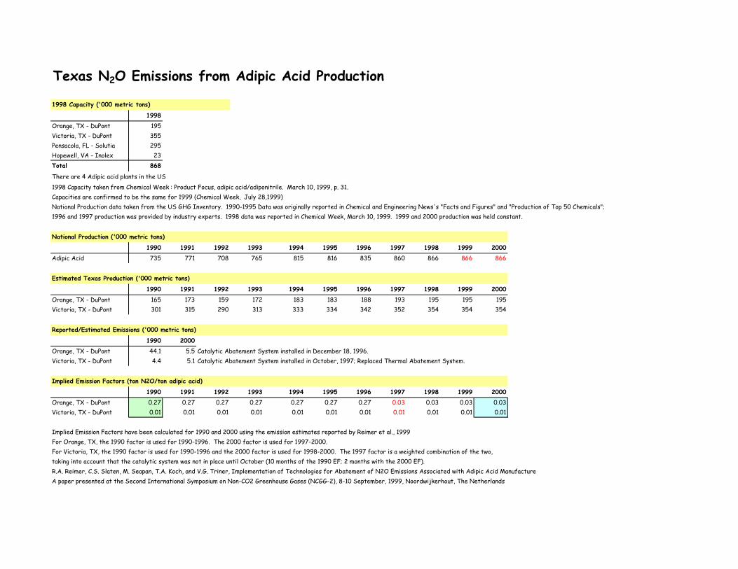
Texas N2O Emissions from Adipic Acid Production

1998 Capacity ('000 metric tons)

1998Orange, TX - DuPont 195Victoria, TX - DuPont 355Pensacola, FL - Solutia 295Hopewell, VA - Inolex 23Total 868

There are 4 Adipic acid plants in the US1998 Capacity taken from Chemical Week : Product Focus, adipic acid/adiponitrile. March 10, 1999, p. 31.Capacities are confirmed to be the same for 1999 (Chemical Week, July 28,1999)National Production data taken from the US GHG Inventory. 1990-1995 Data was originally reported in Chemical and Engineering News's "Facts and Figures" and "Production of Top 50 Chemicals"; 1996 and 1997 production was provided by industry experts. 1998 data was reported in Chemical Week, March 10, 1999. 1999 and 2000 production was held constant.

National Production ('000 metric tons)

1990 1991 1992 1993 1994 1995 1996 1997 1998 1999 2000Adipic Acid 735 771 708 765 815 816 835 860 866 866 866

Estimated Texas Production ('000 metric tons)

1990 1991 1992 1993 1994 1995 1996 1997 1998 1999 2000Orange, TX - DuPont 165 173 159 172 183 183 188 193 195 195 195Victoria, TX - DuPont 301 315 290 313 333 334 342 352 354 354 354

Reported/Estimated Emissions ('000 metric tons)

1990 2000Orange, TX - DuPont 44.1 5.5 Catalytic Abatement System installed in December 18, 1996.Victoria, TX - DuPont 4.4 5.1 Catalytic Abatement System installed in October, 1997; Replaced Thermal Abatement System.

Implied Emission Factors (ton N2O/ton adipic acid)

1990 1991 1992 1993 1994 1995 1996 1997 1998 1999 2000Orange, TX - DuPont 0.27 0.27 0.27 0.27 0.27 0.27 0.27 0.03 0.03 0.03 0.03Victoria, TX - DuPont 0.01 0.01 0.01 0.01 0.01 0.01 0.01 0.01 0.01 0.01 0.01

Implied Emission Factors have been calculated for 1990 and 2000 using the emission estimates reported by Reimer et al., 1999For Orange, TX, the 1990 factor is used for 1990-1996. The 2000 factor is used for 1997-2000.For Victoria, TX, the 1990 factor is used for 1990-1996 and the 2000 factor is used for 1998-2000. The 1997 factor is a weighted combination of the two, taking into account that the catalytic system was not in place until October (10 months of the 1990 EF; 2 months with the 2000 EF). R.A. Reimer, C.S. Slaten, M. Seapan, T.A. Koch, and V.G. Triner, Implementation of Technologies for Abatement of N2O Emissions Associated with Adipic Acid ManufactureA paper presented at the Second International Symposium on Non-CO2 Greenhouse Gases (NCGG-2), 8-10 September, 1999, Noordwijkerhout, The Netherlands

N2O Emissions

'000 metric tons 1990 1991 1992 1993 1994 1995 1996 1997 1998 1999 2000Orange, TX - DuPont 44.10 46.26 42.48 45.90 48.90 48.96 50.10 5.46 5.50 5.50 5.50Victoria, TX - DuPont 4.40 4.62 4.24 4.58 4.88 4.88 5.00 5.13 5.10 5.10 5.10Total 48.50 50.88 46.72 50.48 53.78 53.84 55.10 10.60 10.60 10.60 10.60

GWP of N2O 310

MMTCDE 1990 1991 1992 1993 1994 1995 1996 1997 1998 1999 2000Orange, TX - DuPont 13.67 14.34 13.17 14.23 15.16 15.18 15.53 1.69 1.71 1.71 1.71Victoria, TX - DuPont 1.36 1.43 1.31 1.42 1.51 1.51 1.55 1.59 1.58 1.58 1.58Total 15.04 15.77 14.48 15.65 16.67 16.69 17.08 3.28 3.29 3.29 3.29

MMTCE 1990 1991 1992 1993 1994 1995 1996 1997 1998 1999 2000Orange, TX - DuPont 3.73 3.91 3.59 3.88 4.13 4.14 4.24 0.46 0.47 0.47 0.47Victoria, TX - DuPont 0.37 0.39 0.36 0.39 0.41 0.41 0.42 0.43 0.43 0.43 0.43Total 4.10 4.30 3.95 4.27 4.55 4.55 4.66 0.90 0.90 0.90 0.90

N2O Emissions from Adipic Acid Production in Texas, 1990-1999

0.0

0.5

1.0

1.5

2.0

2.5

3.0

3.5

4.0

4.5

5.0

1990 1991 1992 1993 1994 1995 1996 1997 1998 1999 2000

Year

N2O

Em

ission

s

0

100

200

300

400

500

600

700

800

900

1000

Adi

pic

Acid

Prod

uced

('0

00

met

ric

tons

)

"N2O Emissions" Adipic Acid Produced

Methane Emissions for the Natural Gas Industry - Activity Data

Activity Data 1990 1991 1992 1993 1994 1995 1996 1997 1998 1999 2000

Total Number of Oil Wells 188,829 192,459 185,740 181,501 179,643 174,527 175,532 174,670 163,232 155,849 160,733Number of Wells - Associated (oil wells with gas production) 87,050 88,724 85,626 83,672 82,815 80,457 80,920 80,523 75,250 71,846 74,098Number of Wells - Non-Associated (natural gas wells) 50,867 47,615 46,298 47,101 48,654 54,635 53,816 56,747 58,736 58,712 59,234Number of Off-Shore PlatformsMiles of Gathering Pipeline 4,450 4,450 4,450 4,450 4,450 4,450 4,450 4,450 4,450 4,450 4,450

Number of Gas Processing Plants 285 276 267 259 250 241 236 229 198 202 205

Number of Gas Transmission Stations 108 108 108 108 108 108 108 108 108 108 108Number of Gas Storage Stations 35 35 35 35 35 35 35 35 35 35 35Miles of Transmission Pipeline 36,354 36,354 36,354 36,354 36,354 36,354 36,354 36,354 36,354 36,354 36,354

Miles of Cast Iron Distribution Pipeline 4,818 4,424 4,030 3,434 3,401 3,181 2,452 1,977 1,237 1,164 1,203Miles of Steel Distribution Pipeline 109,964 96,937 90,219 59,994 60,713 49,564 48,751 49,355Miles of Unprotected Steel Distribution Pipeline 19,731 18,327 16,923 16,495 14,541 13,533 8,999 9,107 7,435 7,313 7,403Miles of Protected Steel Distribution Pipeline 111,811 103,853 95,895 93,469 82,396 76,686 50,995 51,606 42,129 41,438 41,952Miles of Plastic Distribution Pipeline 70,469 66,922 63,374 65,016 55,882 55,669 40,709 43,187 38,057 39,268 41,512

Methane Emissions for Oil Activities - Activity Data

Activity Data 1990 1991 1992 1993 1994 1995 1996 1997 1998 1999 2000

Oil Production (bbls) 647,808,621 648,376,775 614,377,142 576,855,119 542,869,512 514,369,729 499,749,861 490,850,893 459,249,421 408,781,188 400,740,722Oil & Gas: Venting/Flared (MMCF) 28,247 30,638 19,689 34,486 42,037 46,183 45,382 47,922 25,811 35,006 27,073

Assumptions & Conversion Factors SourceProportion of total oil wells that are associated (i.e., produce gas) 46% Ratio is based on Natural Gas Inventory data for U.S.Proportion of steel distribution pipeline that is protected 85% Ratio is based on Natural Gas Inventory data for U.S.Proportion of steel distribution pipeline that is unprotected 15% Ratio is based on Natural Gas Inventory data for U.S.Lbs / metric ton 2,204 bbl) 5.8 Table A.2. Approximate Heat Content of Crude Oil, Crude Oil Products, and Natural Gas Plant Liquids,1949-2000, EIA, Annual Energy Review 2000Heating Value, Oil & Gas: Venting & Flaring (BTU/ cf) 1,027 Assumption: Use heating value for natural gas. Source: Table A.4. Approximate Heat Content of Natural Gas,1949-2000, EIA, Annual Energy Review 2000

Source For 1990-1998: Producing Crude Oil Wells, IPAA (December 1999); For 1999: "Texas Distribution of Oil Wells and Production by Rate Bracket", EIA www.eia.doe.gov/pub/oil_gas/petrosystem/petroleum/tx-1a.htm; For 2000: Railroad Commission of Texas, Oil & Gas Division

For 1990-1999: Historical Natural Gas Annual 1930 through 1999, EIA; For 2000: Railroad Commission of Texas, Oil & Gas Division

For 2000: Railroad Commission of Texas, Oil & Gas Division

For 1996-2000: Worldwide Gas Processing, Oil & Gas Journal (June, 1997 through 2001)

For 1998: EIA, Office of Oil and Gas, Reserves and Natural Gas Division's Geographical Information System- Natural Gas CD, 12/3/1998For 1998: EIA, Office of Oil and Gas, Reserves and Natural Gas Division's Geographical Information System- Natural Gas CD, 12/3/1998For 2000: Railroad Commission of Texas, Oil & Gas Division

For 1993-2000: DOT, Office of Pipeline Safety - http://ops.dot.gov/DT98.htmFor 1993-2000: DOT, Office of Pipeline Safety - http://ops.dot.gov/DT98.htm

For 1993-2000: DOT, Office of Pipeline Safety - http://ops.dot.gov/DT98.htm

For 1990-1999: Texas Distribution of Oil Wells and Production by Rate Bracket, EIA - www.eia.doe.gov/pub/oil_gas/petrosystem/petroleum/tx-1a.htm; For 2000: Railroad Commission of Texas, Oil & Gas DivisionFor 1990-1999: Historical Natural Gas Annual 1967 through 1999, Table 5, EIA; For 2000: Railroad Commission of Texas, Oil & Gas Division

Table A.2. Approximate Heat Content of Crude Oil, Crude Oil Products, and Natural Gas Plant Liquids,1949-2000, EIA, Annual Energy Review 2000

Assumption: Use heating value for natural gas. Source: Table A.4. Approximate Heat Content of Natural Gas,1949-2000, EIA, Annual Energy Review 2000

Greenhouse Gases - Amazon Simple Storage Service · 2014-07-10 · about greenhouse gases including...

Documents

Transcript of Greenhouse Gases - Amazon Simple Storage Service · 2014-07-10 · about greenhouse gases including...