GREENHOUSE GAS SEQUESTRATION BY ALGAE – ENERGY AND GREENHOUSE GAS LIFE CYCLE

STUDIES

Peter K. Campbell, Tom Beer, David Batten

Transport Biofuels Stream, CSIRO Energy Transformed Flagship PB1, Aspendale, Vic. 3195, Australia

http://www.csiro.au/org/EnergyTransformedFlagship.html

Email: tom.beer@csiro.au

ABSTRACT We have examined various scenarios involving the growth of algae and the sequestering of carbon during its growth. End-uses for algae are found in the production of food supplements for humans; animal feed; oil extraction and its transesterification to produce biodiesel; electricity production upon combustion directly or by transforming the algae to methane anaerobically; or fuel production via pyrolysis, gasification or anaerobic digestion. In every case, the greenhouse gases sequestered by the algae are released into the atmosphere, so that greenhouse gas benefits arise only as offsets when the algal use displaces the combustion of a fossil fuel in a vehicle or for the production of electricity. This paper examines the greenhouse gas, costs and energy balance on a life-cycle basis for algae grown in salt-water ponds and used to produce biodiesel and electricity. Under the conditions described and the data assumed, it is shown that it is possible to produce algal biodiesel at less cost and with a substantial greenhouse gas and energy balance advantage over fossil diesel. However, when scaled up to large commercial production levels, the costs may exceed those for fossil diesel. The economic viability is highly dependent upon algae with high oil yields capable of high production year-round, which has yet to be demonstrated on a commercial scale.

Keywords: algae, biofuels, biodiesel, emissions, greenhouse gas, green electricity 1. INTRODUCTION The idea of producing liquid or gaseous fuels from algae emerged during the oil crises of the 1970s and led to a significant research and development in the United States [1] and in Australia [2, 3]. In recent years the same idea has received renewed impetus as a result of high oil prices and the perceived opportunity to use biofuels as a method of greenhouse gas reduction [4, 5].

There is a view that if it were possible to capture carbon dioxide flue gases from a power station and use the gases to grow algae for biofuels production then this process would qualify as a carbon capture mechanism. This view is partly correct, since the permissible carbon credits do not arise from the flue gas that is captured because the algae-derived fuel will eventually be burnt and the captured carbon returned to the atmosphere. The carbon credits arise as a result of the displacement of the fossil fuel that would have been used if the biofuel had not become available.

Because of this it is necessary to undertake detailed life-cycle calculations of the processing energy needed to make the biofuel, in order to quantify the greenhouse gas emissions at each stage of the process. This allows us to determine whether the process does indeed emit less CO2 than the use of fossil fuels and if this is the case to quantify the associated carbon credits.

2

This paper examines the social, economic and environmental aspects of one possible method of producing biodiesel on a life-cycle basis. Because much of the detailed mechanics of the operation of commercial algal farms is considered to be confidential proprietary information, we have used the design variables of Regan and Gartside [2] and Benemann and Oswald [4] to estimate the triple bottom line outcomes associated with their design. Since we regard some of the design assumptions described in the abovementioned papers as too idealistic, we have modified some of their assumptions and examined configurations that more closely approximate the likely conditions that would be realized in such algal facilities if they were built today in specifically selected sites within Australia.

2. MICROALGAE

Certain species of microalgae offer the possibility of sustainable, low GHG (greenhouse gas) emissions.

Some of their perceived advantages of microalgae are that they grow rapidly, yield significantly more biofuel per hectare than oil plants, can sequester excess carbon dioxide as hydrocarbons, produce a fuel that contains no sulphur with low toxicity that is highly biodegradable, does not compete significantly with food, fibre or other uses and does not involve destruction of natural habitats. Microalgae contain lipids and fatty acids as membrane components, storage products, metabolites and sources of energy. When grown under standard, nutrient-replete conditions, they show large differences in percentages of the key macronutrients: by dry weight, typically 25 to 40% of protein, 5 to 30% of carbohydrate and 10 to 30% of lipids/oils. Species containing considerably higher oil content have been found and more than a dozen algal species have been mentioned as possible candidates for producing biodiesel.

Microalgae, which many geologists believe produced most fossil fuels in the first place, need light, nutrients and warmth to grow. This occurs naturally on larger scales in bogs, marshes and swamps, salt marshes and salt lakes. Smaller-scale sources include wastewater treatment ponds, animal waste and other liquid wastes. When algal growth conditions exist, the steps involved in producing biodiesel from the algae are shown below. Microalgae are diverse, pervasive, productive and less competitive with other plants as a source of food for human consumption. Though microalgae are aquacultured widely to produce various high-value foods, nutraceuticals and chemicals, the methods adopted have not yet been shown to be economically and ecologically viable for the production of biodiesel in quantities large enough to replace fossil fuels.

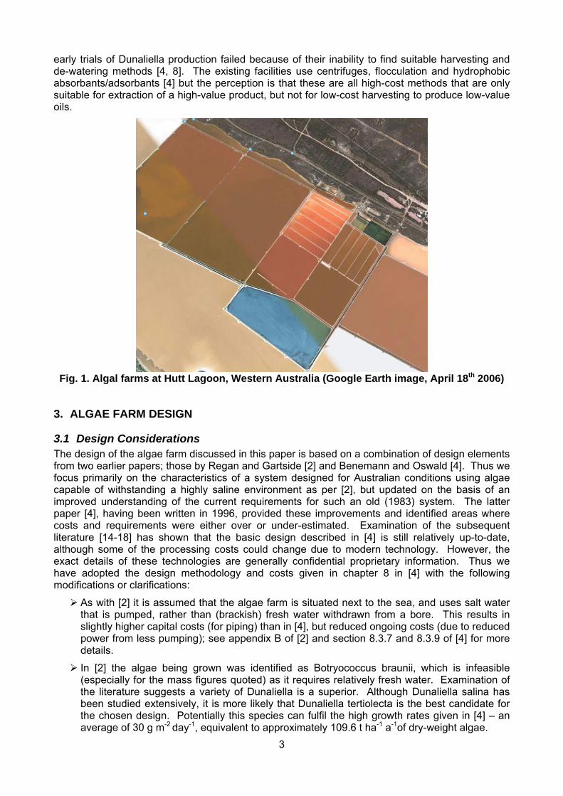
2.1 Existing Australian microalgae production A number of locations exist in Australia where unwanted algal blooms have developed as a result of eutrophication. For example, such blooms have been a problem in the Peel Inlet system of Western Australia for over thirty years [6]. Algae also grow in sewage treatment ponds.

There are, however, two Australian algal farms in commercial operation; one at Hutt Lagoon in Western Australia, and one just north of Whyalla in South Australia. Fig. 1 shows an image of the Hutt Lagoon facility (obtained using Google Earth). Both farms are owned by Cognis, and extract β-carotene from Dunaliella salina [7, 8], which is a green halophilic flagellate. It is estimated [7] that worldwide annual production of Dunaliella salina is 1200 tonne dry weight, and that the two Australian farms cover 800 ha – though [4] estimated that in 1996 the Western Australian ponds covered only 120 ha whereas the South Australian ponds exceeded 300 ha. These estimates indicate a productivity of around 1.5 tonne ha-1 a-1.

2.2 Pond design and operational issues Benemann and Oswald [4] note that the Australian β-carotene production facilities are based on unmixed ponds, whereas the considerably smaller Southern Californian and Israeli ponds (6 ha and 5 ha respectively) are based on raceway ponds with paddle-wheel mixing. Curtain [8] points out that a low cost harvesting method is critical to the economic viability of production. Numerous

3

early trials of Dunaliella production failed because of their inability to find suitable harvesting and de-watering methods [4, 8]. The existing facilities use centrifuges, flocculation and hydrophobic absorbants/adsorbants [4] but the perception is that these are all high-cost methods that are only suitable for extraction of a high-value product, but not for low-cost harvesting to produce low-value oils.

Fig. 1. Algal farms at Hutt Lagoon, Western Australia (Google Earth image, April 18th 2006)

3. ALGAE FARM DESIGN

3.1 Design Considerations The design of the algae farm discussed in this paper is based on a combination of design elements from two earlier papers; those by Regan and Gartside [2] and Benemann and Oswald [4]. Thus we focus primarily on the characteristics of a system designed for Australian conditions using algae capable of withstanding a highly saline environment as per [2], but updated on the basis of an improved understanding of the current requirements for such an old (1983) system. The latter paper [4], having been written in 1996, provided these improvements and identified areas where costs and requirements were either over or under-estimated. Examination of the subsequent literature [14-18] has shown that the basic design described in [4] is still relatively up-to-date, although some of the processing costs could change due to modern technology. However, the exact details of these technologies are generally confidential proprietary information. Thus we have adopted the design methodology and costs given in chapter 8 in [4] with the following modifications or clarifications:

As with [2] it is assumed that the algae farm is situated next to the sea, and uses salt water that is pumped, rather than (brackish) fresh water withdrawn from a bore. This results in slightly higher capital costs (for piping) than in [4], but reduced ongoing costs (due to reduced power from less pumping); see appendix B of [2] and section 8.3.7 and 8.3.9 of [4] for more details.

In [2] the algae being grown was identified as Botryococcus braunii, which is infeasible (especially for the mass figures quoted) as it requires relatively fresh water. Examination of the literature suggests a variety of Dunaliella is a superior. Although Dunaliella salina has been studied extensively, it is more likely that Dunaliella tertiolecta is the best candidate for the chosen design. Potentially this species can fulfil the high growth rates given in [4] – an average of 30 g m-2 day-1, equivalent to approximately 109.6 t ha-1 a-1of dry-weight algae.

4

The flue gas requirements (due to atmospheric CO2 not providing enough carbon for the algae to achieve maximum growth) from [4] have been adopted, which are 83.5% higher than in [2]. See the Appendix for the detailed reasoning behind this choice.

Power requirements for pumping the flue gas have been corrected. In [4] it is indicated that the power requirement is based on a large degree of interpolation; it turns out that the figures are overstated – see the Appendix for details. Although the gas volumes quoted are used, the power requirements are interpolated from [1]. For the ‘base case’, this is 2470 kWh per hectare per year for pumping the flue gas, or 370 kWh per hectare per year for pumping pure CO2 from a nearby ammonia plant (see below).

In [4] two cases for introducing appropriate levels of carbon dioxide to the algae are presented, without which growth rates would be an order of magnitude less. The first is flue gas (15% CO2) from a nearby power station (2.5 km away), the second from pure CO2 delivered to the algae farm. The means of delivery for the CO2 in the second case is ignored in [4]; in reality it would require a large number of trucks (or rail/shipping), as well as additional infrastructure locally to hold a several days worth of compressed (liquefied) gas, and the power required to keep it liquefied. Costs may have been underestimated, assuming an urban delivery charge for the CO2 whereas in reality most power station locations would require a 200 km round-trip. Estimates for these additions have been included. Also presented in this paper is a third case where the algae farm is situated adjacent to a producer of pure CO2. An Australian example is the Ammonia-Urea plant on the Burrup Peninsula in NW Western Australia, which produces 1.4 Mt of carbon dioxide per year – enough to sustain 19 algal farms of 400 ha each [9, 10].

Based on the discussion in [2] and [4] minimum and maximum estimates are assigned to each value to facilitate sensitivity analysis. Furthermore, an extreme ‘sensitivity analysis’ is performed, as both the pipe lengths given in [4] and the algae production rates given in [2] and [4] appear to be overly optimistic. Therefore these have been altered to mimic a more realistic situation reflecting what would happen for extended commercial production of algal biofuel in open saltwater ponds. The initial scenarios are referred to later as the ‘ideal cases’, with the modifications to show the effect of reduced algae production rates and increased pipe lengths denoted as ‘realistic’.

3.2 Design Details A summary of the algae farm design used for this paper follows in this section. The base scenarios with high rates of algal growth and minimal piping infrastructure are denoted as the ‘ideal case’ later on in this paper.

As per [2] 400 ha of shallow growth ponds are constructed on approximately 500ha of flat coastal land, 2.5 km from a coal-fired power station. Suitable Australian locations of a single algae farm have been identified in [2] as being Mackay, Rockhampton, Gladstone (all in Queensland), Dry Creek, Port Augusta, Whyalla (all in South Australia), Port Hedland, Broome and Kununurra (all in Western Australia).

Although finding enough land for one algae farm of this configuration is easy, scaling up is a problem. None of the above sites have sufficient land nearby to build enough algae farms to utilise all of the carbon dioxide outputs of the power stations in question without increasing the piping distance to 50km or more. As shown later, this increased infrastructure cost can substantially impact the viability of the algae farm from an economic perspective, and also affect its greenhouse credentials (due to increased power requirements for pumping the flue gas the extra distance).

The major design elements are:

Construction of the 0.7-1 metre deep growth ponds (containing water to a depth of about 30 cm) including site clearing, grading, levelling, and the construction of channel dividers (berms). Ponds are designed in modules, with the basic design element being two trenches running in parallel, separated by a berm (a mound of earth with a level top that acts as a divider) except for the ends which are connected in a semi-circle to allow water to flow continuously. This is known as a ‘raceway’ design. The ponds are unlined, as plastic liners

5

can double the infrastructure cost. However, the pond bottom is compacted, and in areas with very sandy soil a thin layer of clay is applied; [4] suggests that this should be all that is required for most of the pond area due to self-sealing. Erosion is restricted primarily to pond walls and bases near the paddle wheels (see below), and the berms which are accessible to the elements, so geotextiles (‘Polyfelt’ or similar material) are placed along and over the pond perimeter and exposed areas (including the berms) near the ponds, in addition to the pond bottom near the paddle wheels.

One paddle wheel per raceway is used to ensure a flow rate of 10-25 cm s-1; this ensures a suitable amount of mixing of nutrients and carbon dioxide in the water, as well as avoiding silt suspension and sedimentation of organic solids, according to [4].

Each raceway also has a sump with a baffle through which carbon dioxide is pumped. The pond is also made deeper at this point to ensure 95% or more of the carbon dioxide is absorbed; this requires a water depth of about 1.5 metres. This carbon dioxide is supplied either by pipe from a nearby power station (filtered flue gas), from an ammonia plant (pure carbon dioxide), or from a tank onsite which stores pure carbon dioxide that has been delivered by road in cryogenic tankers (or possibly by rail or ship) in cooled, liquefied form.

A suitable amount of sea water is pumped from the nearby coast to offset losses due to transpiration and evaporation (allowing for inputs from rainfall). After harvesting the waste water (which generally contains concentrated levels of salt), flows via gravity back to sea after treatment.

For harvesting purposes a chemical (hydrophobic polymer) flocculant is used to concentrate algae, which is then fed into a DAF (dissolved air flotation) system to further concentrate the algae, before it is heated and fed into a centrifuge. This concentrates the algae, removes the majority of the remaining water, and extracts the lipids (oil/fat). A centrifuge system is expensive (both in capital and ongoing power & maintenance costs), and many companies are testing cheaper alternatives. It is in this part of the algae farm design that the highest potential for cost reductions occurs.

The lipids are transesterified by combining with alcohol and a catalyst such as potassium hydroxide to produce biodiesel. This process is used for the production of biodiesel from any vegetable oil, such as canola.

Whereas in [2] the remaining algal mass is fed back into the ponds to provide nutrient recycling, in [4] it is moved into an anaerobic digestion unit; basically a covered lagoon. This would result in methane capable of producing 1336.5 GJ of heat energy – see the Appendix for details.

This methane is turned into electricity, either by feeding it back through the piping to the nearby power station (or ammonia plant), during the night when the algae are quiescent and do not have need of the extra CO2, or by the use of a 5MW generator (rather than the 4MW calculated in [4]). A generator/power plant efficiency of 32% is assumed (consistent with the literature on current coal-fired power plants), but is conservative given advances in modern generators1. Similarly it has been reported that coal-fired power stations are noticeably more efficient2, with the most efficient supercritical steam plants today having a 45% thermal efficiency, which could rise to 60% with the next generation of technology. Thus figures for the amount of electricity produced from methane in this paper are likely to be conservative. Being a flammable gas there will possibly be additional costs to ensure that the piping infrastructure is safe for pumping the methane back at night, but if so these have been ignored in [4]. As such they are also ignored in this paper.

1 At http://tinyurl.com/6y69va it is reported that 1.8 MW gas generators of 40% efficiency are commercially available; efficiencies of 35-45% are commonly reported on company websites for newer 1-10 MW gas turbine generators. 2 See http://www.australiancoal.com.au/environmentfuture.htm, for example.

6

This electricity is used to offset power requirements of the algae farm, with the excess being fed back into the grid. For purposes of the life cycle analysis, however, it is assumed that all the electricity produced is fed back into the grid – which is effectively the case for the power station. A problem occurs with the stationing of a generator at the algae farm (and also potentially the ammonia plant) which is ignored in [4]; there is a requirement for a switching facility and additional plant capital to properly link the power back into the local grid.

As mentioned above, no algal mass is fed back into the ponds (as suggested in [2]) to recycle nutrients. Thus substantial amounts of nitrogen and phosphorus (in the form of ammonia, urea and superphosphate fertilisers) and small amounts of iron (iron sulphate fertiliser) need to be added regularly to the algae ponds, in addition to the carbon dioxide.

The algae farm also requires the construction of roads, drainage and buildings, electrical supply and distribution, instrumentation, machinery (including vehicles). Also people are required to run the facility (including the administrative staff not directly operating the plant, but necessary for the function of the facility).

Given the amount of electricity produced by the algae farm with the above design, it is perhaps more accurate to think of it as a biogas power plant that produces biodiesel as a by-product, rather than the other way around. This is not uncommon among the several designs that have been evaluated by CSIRO scientists. In each case, biodiesel was a by-product among several liquid or gaseous fuels produced by the proposed facilities.

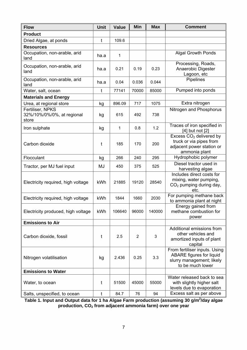
The input and output data for a hectare of algal farm production using the above design with an adjacent ammonia plant are shown in Table 1. Note that “ha.a” values indicate the use of a hectare of land over the course of one year (annum). The electricity values vary between the different cases. More electricity is required for pumping in the flue gas case (with only 15% of the flue gas being CO2). Proportionally less pumping is required for the ammonia plant case (as the gas is pure CO2). These costs are not incurred when CO2 is trucked in, but in this case there are additional emissions to the air from these delivery trucks and the initial production of the CO2 (which would otherwise be a waste product from the flue gas case).

Additional inputs are required to transform the dried algae into oil, as described in the Appendix.

7

Flow Unit Value Min Max Comment Product Dried Algae, at ponds t 109.6 Resources Occupation, non-arable, arid land ha.a 1 Algal Growth Ponds

Occupation, non-arable, arid land ha.a 0.21 0.19 0.23

Processing, Roads, Anaerobic Digester

Lagoon, etc Occupation, non-arable, arid land ha.a 0.04 0.036 0.044 Pipelines

Water, salt, ocean t 77141 70000 85000 Pumped into ponds Materials and Energy Urea, at regional store kg 896.09 717 1075 Extra nitrogen Fertiliser, NPKS 32%/10%/0%/0%, at regional store

kg 615 492 738 Nitrogen and Phosphorus

Iron sulphate kg 1 0.8 1.2 Traces of iron specified in [4] but not [2]

Carbon dioxide t 185 170 200

Excess CO2 delivered by truck or via pipes from

adjacent power station or ammonia plant

Flocculant kg 266 240 295 Hydrophobic polymer

Tractor, per MJ fuel input MJ 450 375 525 Diesel tractor used in harvesting algae

Electricity required, high voltage kWh 21885 19120 28540

Includes direct costs for mixing, water pumping,

CO2 pumping during day, etc.

Electricity required, high voltage kWh 1844 1660 2030 For pumping methane back to ammonia plant at night

Electricity produced, high voltage kWh 106640 96000 140000 Energy gained from

methane combustion for power

Emissions to Air

Carbon dioxide, fossil t 2.5 2 3

Additional emissions from other vehicles and

amortized inputs of plant capital

Nitrogen volatilisation kg 2.436 0.25 3.3

From fertiliser inputs. Using ABARE figures for liquid

slurry management; likely to be much lower

Emissions to Water

Water, to ocean t 51500 45000 55000 Water released back to sea

with slightly higher salt levels due to evaporation

Salts, unspecified, to ocean t 84.7 76 94 Excess salt as per above Table 1. Input and Output data for 1 ha Algae Farm production (assuming 30 g/m2/day algae

production, CO2 from adjacent ammonia farm) over one year

8

4. ENVIRONMENTAL ANALYSIS

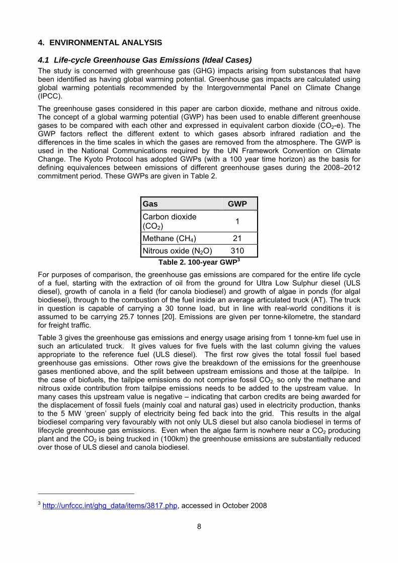
4.1 Life-cycle Greenhouse Gas Emissions (Ideal Cases) The study is concerned with greenhouse gas (GHG) impacts arising from substances that have been identified as having global warming potential. Greenhouse gas impacts are calculated using global warming potentials recommended by the Intergovernmental Panel on Climate Change (IPCC).

The greenhouse gases considered in this paper are carbon dioxide, methane and nitrous oxide. The concept of a global warming potential (GWP) has been used to enable different greenhouse gases to be compared with each other and expressed in equivalent carbon dioxide (CO2-e). The GWP factors reflect the different extent to which gases absorb infrared radiation and the differences in the time scales in which the gases are removed from the atmosphere. The GWP is used in the National Communications required by the UN Framework Convention on Climate Change. The Kyoto Protocol has adopted GWPs (with a 100 year time horizon) as the basis for defining equivalences between emissions of different greenhouse gases during the 2008–2012 commitment period. These GWPs are given in Table 2.

Gas GWP Carbon dioxide (CO2)

1

Methane (CH4) 21 Nitrous oxide (N2O) 310

Table 2. 100-year GWP3 For purposes of comparison, the greenhouse gas emissions are compared for the entire life cycle of a fuel, starting with the extraction of oil from the ground for Ultra Low Sulphur diesel (ULS diesel), growth of canola in a field (for canola biodiesel) and growth of algae in ponds (for algal biodiesel), through to the combustion of the fuel inside an average articulated truck (AT). The truck in question is capable of carrying a 30 tonne load, but in line with real-world conditions it is assumed to be carrying 25.7 tonnes [20]. Emissions are given per tonne-kilometre, the standard for freight traffic.

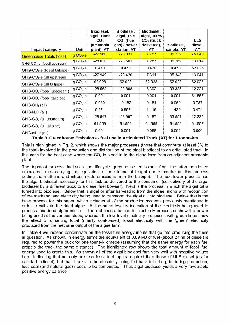
Table 3 gives the greenhouse gas emissions and energy usage arising from 1 tonne-km fuel use in such an articulated truck. It gives values for five fuels with the last column giving the values appropriate to the reference fuel (ULS diesel). The first row gives the total fossil fuel based greenhouse gas emissions. Other rows give the breakdown of the emissions for the greenhouse gases mentioned above, and the split between upstream emissions and those at the tailpipe. In the case of biofuels, the tailpipe emissions do not comprise fossil CO2, so only the methane and nitrous oxide contribution from tailpipe emissions needs to be added to the upstream value. In many cases this upstream value is negative – indicating that carbon credits are being awarded for the displacement of fossil fuels (mainly coal and natural gas) used in electricity production, thanks to the 5 MW ‘green’ supply of electricity being fed back into the grid. This results in the algal biodiesel comparing very favourably with not only ULS diesel but also canola biodiesel in terms of lifecycle greenhouse gas emissions. Even when the algae farm is nowhere near a CO2 producing plant and the CO2 is being trucked in (100km) the greenhouse emissions are substantially reduced over those of ULS diesel and canola biodiesel.

3 http://unfccc.int/ghg_data/items/3817.php, accessed in October 2008

9

Impact category Unit

Biodiesel, algal, 100%

CO2 (ammonia plant), AT

Biodiesel, algal, 15% CO2 (flue

gas) - power station, AT

Biodiesel, algal, 100% CO2 (truck delivered),

AT Biodiesel, canola, AT

ULS diesel,

AT

Greenhouse Totals (fossil) g CO2-e -27.560 -23.031 7.757 35.739 75.040

GHG-CO2-e (fossil upstream) g CO2-e -28.030 -23.501 7.287 35.269 13.014

GHG-CO2-e (fossil tailpipe) g CO2-e 0.470 0.470 0.470 0.470 62.026

GHG-CO2-e (all upstream) g CO2-e -27.949 -23.420 7.311 35.348 13.041

GHG-CO2-e (all tailpipe) g CO2-e 62.028 62.028 62.028 62.028 62.026

GHG-CO2 (fossil upstream) g CO2-e -28.563 -23.808 6.392 33.335 12.221

GHG-CO2 (fossil tailpipe) g CO2-e 0.001 0.001 0.001 0.001 61.557

GHG-CH4 (all) g CO2-e 0.030 -0.182 0.181 0.969 0.787

GHG-N2O (all) g CO2-e 0.971 0.957 1.116 1.430 0.474

GHG-CO2 (all upstream) g CO2-e -28.547 -23.997 6.187 33.557 12.225

GHG-CO2 (all tailpipe) g CO2-e 61.559 61.559 61.559 61.559 61.557

GHG-other (all) g CO2-e 0.001 0.001 0.068 0.004 0.000

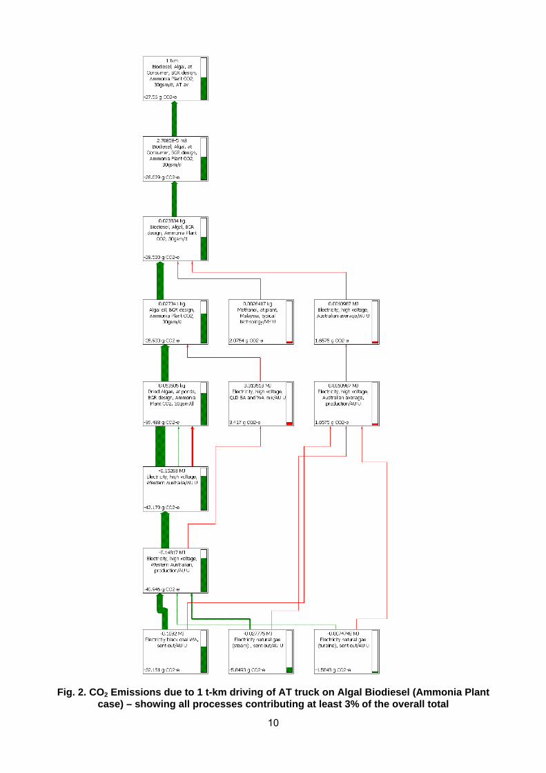
Table 3. Greenhouse Emissions - fuel use in Articulated Truck (AT) for 1 tonne-km This is highlighted in Fig. 2, which shows the major processes (those that contribute at least 3% to the total) involved in the production and distribution of the algal biodiesel to an articulated truck, in this case for the best case where the CO2 is piped in to the algae farm from an adjacent ammonia plant.

The topmost process indicates the lifecycle greenhouse emissions from the aforementioned articulated truck carrying the equivalent of one tonne of freight one kilometre (in this process adding the methane and nitrous oxide emissions from the tailpipe). The next lower process has the algal biodiesel necessary for this task as delivered to the consumer (i.e. delivery of the algal biodiesel by a different truck to a diesel fuel bowser). Next is the process in which the algal oil is turned into biodiesel. Below that is algal oil after harvesting from the algae, along with recognition of the methanol and electricity being used to transform the algal oil into biodiesel. Below that is the base process for this paper, which includes all of the production systems previously mentioned in order to cultivate the dried algae. At the same level is indication of the electricity being used to process this dried algae into oil. The red lines attached to electricity processes show the power being used at the various steps, whereas the low-level electricity processes with green lines show the effect of offsetting local (mainly coal-based) fossil electricity with the ‘green’ electricity produced from the methane output of the algae farm.

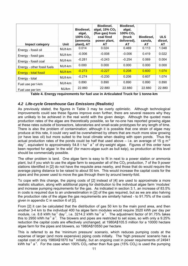
In Table 4 we instead concentrate on the fossil fuel energy inputs that go into producing the fuels in question. As shown, in energy terms the equivalent of 0.89 MJ of fuel (about 27 ml of diesel) is required to power the truck for one tonne-kilometre (assuming that the same energy for each fuel propels the truck the same distance). The highlighted row shows the total amount of fossil fuel energy used to create this. As shown all of the algal biodiesel fare very well with negative values here, indicating that not only are less fossil fuel inputs required than those of ULS diesel (as for canola biodiesel), but that thanks to the electricity being fed back into the grid during production, less coal (and natural gas) needs to be combusted. Thus algal biodiesel yields a very favourable positive energy balance.

10

Fig. 2. CO2 Emissions due to 1 t-km driving of AT truck on Algal Biodiesel (Ammonia Plant

case) – showing all processes contributing at least 3% of the overall total

11

Impact category Unit

Biodiesel, algal,

100% CO2 (ammonia plant), AT

Biodiesel, algal, 15% CO2 (flue gas) from

coal fired power plant,

AT

Biodiesel, algal,

100% CO2 (truck

delivered), AT

Biodiesel, canola,

AT

ULS diesel,

AT

Energy - fossil oil MJ/t-km 0.014 0.024 0.469 0.113 1.048

Energy - fossil gas MJ/t-km -0.006 -0.008 -0.006 0.419 0.022

Energy - fossil coal MJ/t-km -0.281 -0.243 -0.254 0.069 0.004

Energy - other fossil fuels MJ/t-km 0.000 0.000 0.000 0.000 0.000

Energy - total fossil MJ/t-km -0.273 -0.227 0.208 0.600 1.074

Energy - total MJ/t-km -0.274 -0.230 0.206 0.607 1.074

Fuel use per t-km MJ/t-km 0.890 0.890 0.890 0.890 0.890

Fuel use per km MJ/km 22.880 22.880 22.880 22.880 22.880

Table 4. Energy requirements for fuel use in Articulated Truck for 1 tonne-km

4.2 Life-cycle Greenhouse Gas Emissions (Realistic) As previously stated, the figures in Table 3 may be overly optimistic. Although technological improvements could see these figures improve even further, there are several reasons why they are unlikely to be achieved in the real world with the given design. Although the quoted mass production rates of the algae are theoretically possible, so far no-one has reported growing algae at these rates outside of bioreactors, laboratories and small-scale prototypes for any length of time. There is also the problem of contamination; although it is possible that one strain of algae may produce at this rate, it could very well be overwhelmed by others that are much more slow growing (or have less oil) but more suited to the local climate when dealing with open ponds. Thus the actual production rates of the ponds could be half that used above – i.e. an average of 15 g m-2

day-1, equivalent to approximately 54.8 t ha-1 a-1 of dry-weight algae. Figures of this order have been reported for algae ‘in the wild’ (for macro-algae such as bull kelp), so production at this level should be commercially possible.

The other problem is land. One algae farm is easy to fit in next to a power station or ammonia plant, but if you wish to use the algae farm to sequester all of the CO2 production, 7 of the 9 power stations identified in [2] do not have the requisite area nearby, and those that do would require the average piping distance to be raised to about 50 km. This would increase the capital costs for the pipes and the power used to move the gas through them by around twenty-fold.

To cope with this change, the piping costs of [2] instead of [4] are used to approximate a more realistic situation, along with additional piping for distribution to the individual algae farm ‘modules’ and increase pumping requirements for the gas. As indicated in section 3.1, an increase of 83.5% in costs is required due to an underestimation in [2] of the gas required, but as we are also halving the production rate of the algae the gas requirements are similarly halved - to 91.75% of the costs given in appendix C in section 6 of [2].

From [2] it can be calculated that the distribution of gas 50 km to the main pond area, and then another 3-4 km to the individual 400 ha algae farm modules would require 3520 kWh per day per module, i.e. 8.8 kWh ha-1 day-1, i.e. 3214.2 kWh ha-1 a-1. The adjustment factor of 91.75% takes this to 2950 kWh ha-1 a-1. The blowers and pipes are restricted to set sizes, so with only a 9.25% reduction the capital costs are effectively unchanged, at 1980A$105.5 million for a 10000 hectare algae farm for the pipes and blowers, so 1980A$10550 per hectare.

This is referred to as the ‘minimum pressure’ scenario, which reduces pumping costs at the expense of larger (and more expensive) piping costs initially. The ‘high pressure’ scenario has a capital cost of only 1980A$1870 ha-1 initially, but an ongoing cost in power requirements of 24941 kWh ha-1 a-1. For the case when 100% CO2 rather than flue gas (15% CO2) is used the pumping

12

costs of the gas are reduced proportionately down to 482.13 kWh ha-1 a-1. Similarly the cost of piping and blowers can be reduced dramatically as well, conservatively to 1980A$1850 ha-1.

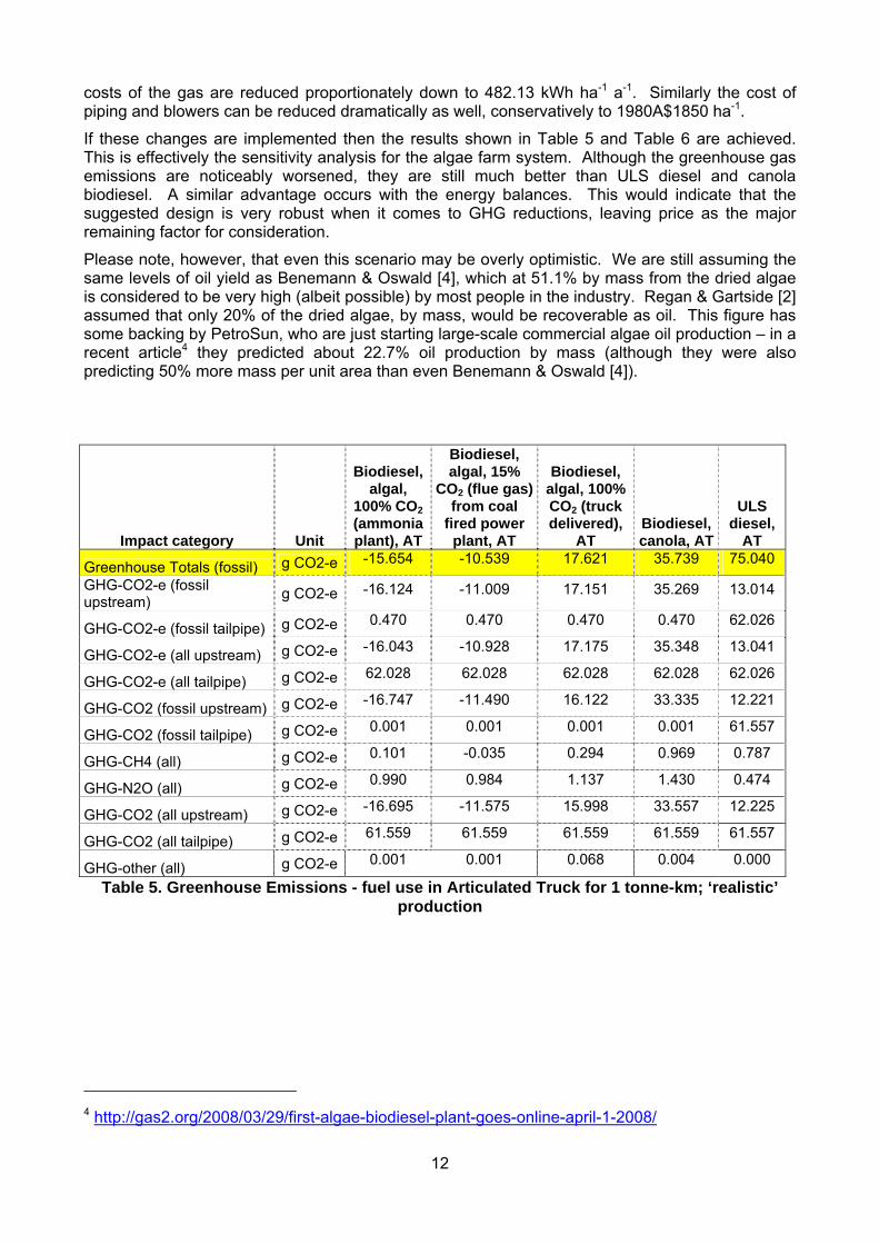
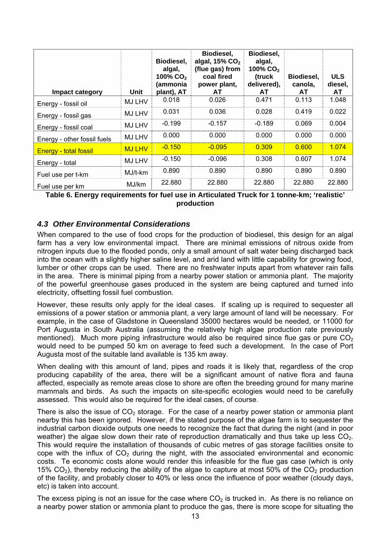
If these changes are implemented then the results shown in Table 5 and Table 6 are achieved. This is effectively the sensitivity analysis for the algae farm system. Although the greenhouse gas emissions are noticeably worsened, they are still much better than ULS diesel and canola biodiesel. A similar advantage occurs with the energy balances. This would indicate that the suggested design is very robust when it comes to GHG reductions, leaving price as the major remaining factor for consideration.

Please note, however, that even this scenario may be overly optimistic. We are still assuming the same levels of oil yield as Benemann & Oswald [4], which at 51.1% by mass from the dried algae is considered to be very high (albeit possible) by most people in the industry. Regan & Gartside [2] assumed that only 20% of the dried algae, by mass, would be recoverable as oil. This figure has some backing by PetroSun, who are just starting large-scale commercial algae oil production – in a recent article4 they predicted about 22.7% oil production by mass (although they were also predicting 50% more mass per unit area than even Benemann & Oswald [4]).

Impact category Unit

Biodiesel, algal,

100% CO2 (ammonia plant), AT

Biodiesel, algal, 15%

CO2 (flue gas) from coal

fired power plant, AT

Biodiesel, algal, 100% CO2 (truck delivered),

AT Biodiesel, canola, AT

ULS diesel,

AT

Greenhouse Totals (fossil) g CO2-e -15.654 -10.539 17.621 35.739 75.040

GHG-CO2-e (fossil upstream) g CO2-e -16.124 -11.009 17.151 35.269 13.014

GHG-CO2-e (fossil tailpipe) g CO2-e 0.470 0.470 0.470 0.470 62.026

GHG-CO2-e (all upstream) g CO2-e -16.043 -10.928 17.175 35.348 13.041

GHG-CO2-e (all tailpipe) g CO2-e 62.028 62.028 62.028 62.028 62.026

GHG-CO2 (fossil upstream) g CO2-e -16.747 -11.490 16.122 33.335 12.221

GHG-CO2 (fossil tailpipe) g CO2-e 0.001 0.001 0.001 0.001 61.557

GHG-CH4 (all) g CO2-e 0.101 -0.035 0.294 0.969 0.787

GHG-N2O (all) g CO2-e 0.990 0.984 1.137 1.430 0.474

GHG-CO2 (all upstream) g CO2-e -16.695 -11.575 15.998 33.557 12.225

GHG-CO2 (all tailpipe) g CO2-e 61.559 61.559 61.559 61.559 61.557

GHG-other (all) g CO2-e 0.001 0.001 0.068 0.004 0.000

Table 5. Greenhouse Emissions - fuel use in Articulated Truck for 1 tonne-km; ‘realistic’ production

4 http://gas2.org/2008/03/29/first-algae-biodiesel-plant-goes-online-april-1-2008/

13

Impact category Unit

Biodiesel, algal,

100% CO2 (ammonia plant), AT

Biodiesel, algal, 15% CO2 (flue gas) from

coal fired power plant,

AT

Biodiesel, algal,

100% CO2 (truck

delivered), AT

Biodiesel, canola,

AT

ULS diesel,

AT

Energy - fossil oil MJ LHV 0.018 0.026 0.471 0.113 1.048

Energy - fossil gas MJ LHV 0.031 0.036 0.028 0.419 0.022

Energy - fossil coal MJ LHV -0.199 -0.157 -0.189 0.069 0.004

Energy - other fossil fuels MJ LHV 0.000 0.000 0.000 0.000 0.000

Energy - total fossil MJ LHV -0.150 -0.095 0.309 0.600 1.074

Energy - total MJ LHV -0.150 -0.096 0.308 0.607 1.074

Fuel use per t-km MJ/t-km 0.890 0.890 0.890 0.890 0.890

Fuel use per km MJ/km 22.880 22.880 22.880 22.880 22.880

Table 6. Energy requirements for fuel use in Articulated Truck for 1 tonne-km; ‘realistic’ production

4.3 Other Environmental Considerations When compared to the use of food crops for the production of biodiesel, this design for an algal farm has a very low environmental impact. There are minimal emissions of nitrous oxide from nitrogen inputs due to the flooded ponds, only a small amount of salt water being discharged back into the ocean with a slightly higher saline level, and arid land with little capability for growing food, lumber or other crops can be used. There are no freshwater inputs apart from whatever rain falls in the area. There is minimal piping from a nearby power station or ammonia plant. The majority of the powerful greenhouse gases produced in the system are being captured and turned into electricity, offsetting fossil fuel combustion.

However, these results only apply for the ideal cases. If scaling up is required to sequester all emissions of a power station or ammonia plant, a very large amount of land will be necessary. For example, in the case of Gladstone in Queensland 35000 hectares would be needed, or 11000 for Port Augusta in South Australia (assuming the relatively high algae production rate previously mentioned). Much more piping infrastructure would also be required since flue gas or pure CO2 would need to be pumped 50 km on average to feed such a development. In the case of Port Augusta most of the suitable land available is 135 km away.

When dealing with this amount of land, pipes and roads it is likely that, regardless of the crop producing capability of the area, there will be a significant amount of native flora and fauna affected, especially as remote areas close to shore are often the breeding ground for many marine mammals and birds. As such the impacts on site-specific ecologies would need to be carefully assessed. This would also be required for the ideal cases, of course.

There is also the issue of CO2 storage. For the case of a nearby power station or ammonia plant nearby this has been ignored. However, if the stated purpose of the algae farm is to sequester the industrial carbon dioxide outputs one needs to recognize the fact that during the night (and in poor weather) the algae slow down their rate of reproduction dramatically and thus take up less CO2. This would require the installation of thousands of cubic metres of gas storage facilities onsite to cope with the influx of CO2 during the night, with the associated environmental and economic costs. Te economic costs alone would render this infeasible for the flue gas case (which is only 15% CO2), thereby reducing the ability of the algae to capture at most 50% of the CO2 production of the facility, and probably closer to 40% or less once the influence of poor weather (cloudy days, etc) is taken into account.

The excess piping is not an issue for the case where CO2 is trucked in. As there is no reliance on a nearby power station or ammonia plant to produce the gas, there is more scope for situating the

14

algae farm in areas likely to have the least environmental impacts. However, there is still a problem with situating the farm as close as possible to the CO2 delivery centre for economic reasons. The amount of trucking involved – over 4 trucks per day for just one 400 hectare farm – is considerable and expensive. Thus some of the algal biodiesel could be best put to use refuelling these gas delivery vehicles. The vehicle-related emissions could also be dramatically reduced is alternative transport (e.g. train or ship) is available for CO2 delivery.

In the anaerobic digester about two-thirds of the solids eventually get converted into biogas. The remaining one-third is a mixture of liquids and solids traditionally treated as a waste product. However, this “bio-sludge” or “bio-slurry” is now gaining favour as an organic fertiliser, and has been used in China in this manner for several years [13]. This offers additional potential benefits and offsets against fossil fuels (nitrogen fertilisers traditionally have extensive natural gas inputs). Since there is insufficient data on the benefits of this slurry as produced from algae, it is instead regarded as a waste product, requiring additional processing.

As previously mentioned, the assumption of 32% efficiency for converting the heat energy of methane into electricity is likely to be conservative (at least for the flue gas case), with modern supercritical steam plants capable of 45% thermal efficiency. Another potential improvement could arise from mixing other feedstocks with coal. For instance, it has been reported2 that co-firing of biomass in conjunction with coal can increased the efficiency of conversion from biomass into electricity from 20% to 35%. The injection of methane into the coal combustion process is another form of co-firing which can potentially increase the efficiency of thermal conversion of both products, leading to even more gains in efficiency, including corresponding decreases in greenhouse gas emissions and more profit from electricity production than is admitted in this paper. More real-world application of this technology is required in order to provide figures that one can be confident in using in this and subsequent papers.

5. ECONOMIC ANALYSIS In this section, costs are compared for the entire life cycle of a fuel, starting with the extraction of oil for Ultra Low Sulphur diesel (for ULS diesel), growth of canola in a field (for canola biodiesel) and growth of algae in ponds (for algal biodiesel). The cycle ends with combustion of the fuel inside an average 30 tonne articulated truck (AT). Capital costs are included, and have been amortized at a rate of 15% per year for the algal biodiesel facility. This rate corresponds to the maximum discount rate allowed by the Australian Tax Office for purposes of tax accounting. If the embodied energy of the infrastructure were to be included in the calculation of greenhouse gas emissions (which it has not been in preceding reports, nor in this one), this should be amortized at a much lower rate, on the order of 6-7% to indicate that it is expected to last at least 20 years. Total costs are given per tonne-kilometre.

Costs for canola biodiesel and ULS diesel are based on the average over September-October 2008, i.e. A$1.65 per litre for ULS diesel, with the canola oil that the biodiesel is based on selling for $1640 per tonne. For canola biodiesel co-products such as animal feed are taken into account.

There are two primary areas where costs did not follow changes in the CPI:

In real terms, construction costs actually dropped over much of the 1990s, before starting to rise again at the beginning of this decade. Based on data from Macromonitor5, the index for 1996 was 91.5, and has risen to 113 in the 12 years since – an overall increase in 23.5%. This is less than CPI over the same period (37.4%) and thus our updated costs have a smaller component due to construction. Forecasts are that construction costs will continue to rise (in real terms) for the next few years, however, so algal plants built in the future may be more expensive in this regard.

5 See http://www.macromonitor.com.au/macromonitor_news_release.pdf, especially p.3 diagram

15

According to McLennan Magasanik Associates6 the average cost for industrial electricity was about 6.4 ¢/kWh in 2002, which translates to about 7.5 ¢/kWh in 2008. Thus electrical costs have dropped in real terms over the last decade. Electricity fed back into the grid is assigned MRET (Mandatory Renewable Energy Target) credits, resulting in an average of 0.5¢ extra per kWh currently, for a total of 8 ¢/kWh. This could increase with the introduction of the national CPRS (Carbon Pollution Reduction Scheme, formerly known as the ETS or Emissions Trading Scheme), currently scheduled for 2010; similarly the base cost of electricity could also rise.

In order to feed a few MW of electricity back into the grid, additional equipment is required in order to handle switching, load balancing and other details. These costs are ignored in [4], but need to be considered for the case where pure CO2 is delivered to the algae farm. If one assumes a cost of one million dollars, this would add about $375 per hectare-year in costs (assuming a 400ha algae farm, and the aforementioned 15% depreciation of plant capital per year). Electricity production results in a payback of $8678.34 per hectare per year (see the Appendix for details). For the cases with an adjacent power station or ammonia plant some of this is lost in pumping it back, resulting in a slightly reduced benefit of $8217.40/ha-a.

Additional profit could be earned from the electricity being fed back into the grid. In this paper it is assumed that the amount paid for this ‘green’ electricity will be slightly higher than the cost of electricity bought, due to the addition of credits from the MRET scheme. Consumers pay around 20 ¢/kWh currently for ‘green’ electricity, so there is substantial scope for an increased payment here.

Additional costs apply for the truck delivered CO2 case. There are operational and maintenance costs for the generator. Benemann et al. [4] suggest this could be as high as 5.1 ¢/kWh, but the California Energy Commission7 suggests 0.45-0.55 ¢/kWh, a mere one tenth the cost. The lower estimate, 0.5 ¢/kWh has been adopted as it is assumed that modern generators are more efficient and require less maintenance.

There is also a requirement for CO2 storage tanks to be built onsite. In order to cope with public holidays and temporary losses in supply, about 4 days worth of gas needs to be stored locally; i.e. about 900 cubic metres. Storage is estimated at a capital cost of A$2.5 million. Power is also required to keep the carbon dioxide cool (it is stored in liquefied form to reduce volume), say about 100 MWh per year. Note that these estimates in particular are very ‘rubbery’ and would require much more detailed analyses before such a system was to be seriously considered for production.

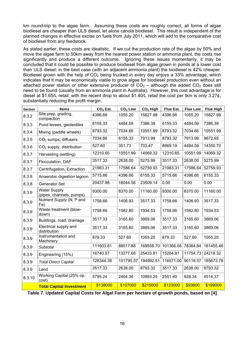
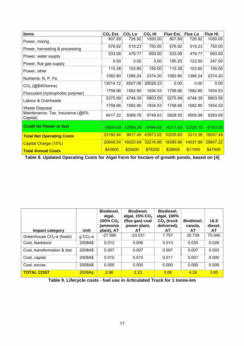
5.1 Economic Analysis (Ideal Cases) Table 7 shows updated capital costs (2008A$) for building the algae farm, based on [4] and the aforementioned alterations. Only the costs for the ‘pure CO2’ case (where the carbon dioxide is delivered) and the ‘flue gas’ case (with flue gas pumped from a nearby power station) are shown here (along with low and high estimates). Costs for pure CO2 delivered from a nearby ammonia plant are nearly identical to the ‘flue gas’ case, other than an 80% reduction in capital costs and 90% reduction in power costs for CO2 supply and distribution. The ‘section’ column indicates the relevant section in [4] that discusses the items in question. Estimates are given for ‘low’ and ‘high’ costs for sensitivity analysis purposes. Table 8 is similar, except that it shows updated operating costs (2008A$) for running the algae farm.

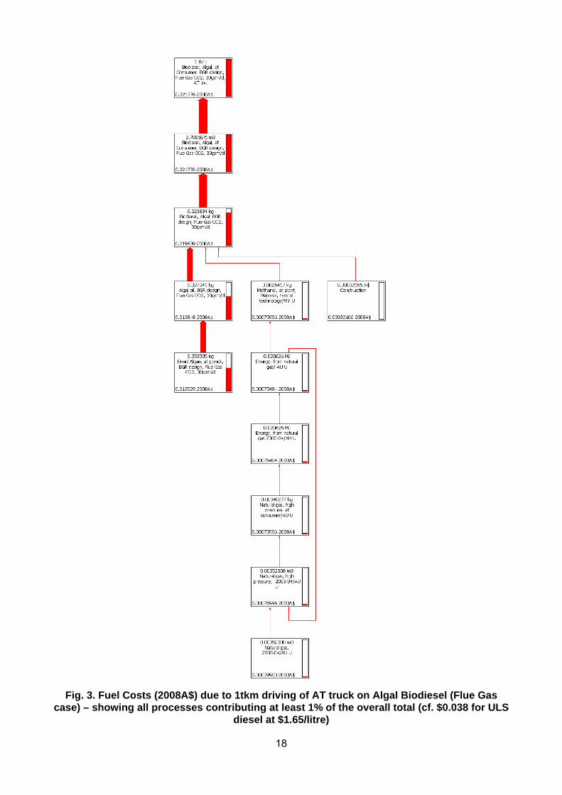
Table 9 shows the lifecycle costs associated with the use of the biodiesel in an articulated truck of 30 tonnes for one tonne-kilometre. Fig. 3 breaks these costs down over individual processes for the flue gas case, as in Fig. 2 but for costs rather than greenhouse gas emissions. Note that the costs for the case with truck delivered CO2 could be underestimated. It is assumed that the cost for CO2 is a delivered cost, but this may only be for urban delivery rather than the estimated 200

6 See http://www.mmassociates.com.au/electricity_publications.html, accessed October 2008 7 http://www.energy.ca.gov/distgen/economics/operation.html, accessed October 2008

16

km round-trip to the algae farm. Assuming these costs are roughly correct, all forms of algae biodiesel are cheaper than ULS diesel, let alone canola biodiesel. This result is independent of the planned changes in effective excise on fuels from July 2011, which will add to the comparative cost of biodiesel from any feedstock.

As stated earlier, these costs are idealistic. If we cut the production rate of the algae by 50% and move the algae farm to 50km away from the nearest power station or ammonia plant, the costs rise significantly and produce a different outcome. Ignoring these issues momentarily, it may be concluded that it could be possible to produce biodiesel from algae grown in ponds at a lower cost than ULS diesel; in the best case (with an adjacent ammonia plant) the biodiesel is 42% cheaper. Biodiesel grown with the help of CO2 being trucked in every day enjoys a 33% advantage, which indicates that it may be economically viable to grow algae for biodiesel production even without an attached power station or other extensive producer of CO2 – although the added CO2 does still need to be found (usually from an ammonia plant in Australia). However, this cost advantage is for diesel at $1.65/L retail; with the recent drop to about $1.40/L retail the cost per tkm is only 3.27¢, substantially reducing the profit margin.

Section Items CO2 Est. CO2 Low CO2 High Flue Est. Flue Low Flue High

8.3.2 Site prep, grading, compaction

4396.66 1055.20 15827.98 4396.66 1055.20 15827.98

8.3.3 Pond levees, geotextiles 6155.33 4484.59 7386.39 6155.33 4484.59 7386.39

8.3.4 Mixing (paddle wheels) 8793.32 7034.66 10551.99 8793.32 7034.66 10551.99

8.3.5 CO2 sumps, diffusers 7034.66 6155.33 7913.99 8793.32 7913.99 9672.65

8.3.6 CO2 supply, distribution 527.60 351.73 703.47 8969.19 4484.59 14350.70

8.3.7 Harvesting (settling) 12310.65 10551.99 14069.32 12310.65 10551.99 14069.32

8.3.7 Flocculation, DAF 3517.33 2638.00 5275.99 3517.33 2638.00 5275.99

8.3.7 Centrifugation, Extraction 21983.31 17586.64 52759.93 21983.31 17586.64 52759.93

8.3.8 Anaerobic digestion lagoon 5715.66 4396.66 6155.33 5715.66 4396.66 6155.33

8.3.8 Generator Set 20437.98 16044.56 23509.14 0.00 0.00 0.00

8.3.9 Water Supply (pipes, channels, pumps)

9300.00 8370.00 11160.00 9300.00 8370.00 11160.00

8.3.9 Nutrient Supply (N, P and Fe)

1758.66 1406.93 3517.33 1758.66 1406.93 3517.33

8.3.9 Waste treatment (blow-down)

1758.66 1582.80 1934.53 1758.66 1582.80 1934.53

8.3.9 Buildings, road, drainage 3517.33 3165.60 3869.06 3517.33 3165.60 3869.06

8.3.9 Electrical supply and distribution

3517.33 3165.60 3869.06 3517.33 3165.60 3869.06

8.3.9 Instrumentation and Machinery

879.33 527.60 1055.20 879.33 527.60 1055.20

8.3.9 Subtotal 111603.81 88517.88 169558.70 101366.08 78364.84 161455.46

8.3.9 Engineering (15%) 16740.57 13277.68 25433.81 15204.91 11754.73 24218.32

8.3.9 Total Direct Capital 128344.38 101795.57 194992.51 116571.00 90119.57 185673.78

8.3.9 Land 3517.33 2638.00 8793.32 3517.33 2638.00 8793.32

8.3.10 Working Capital (25% op. cost)

5795.24 2404.36 10993.25 2551.40 828.34 4514.37

Total Capital Investment $138000 $107000 $215000 $123000 $93600 $199000

Table 7. Updated Capital Costs for Algal Farm per hectare of growth ponds, based on [4]

17

Items CO2 Est. CO2 Lo CO2 Hi Flue Est. Flue Lo Flue Hi

Power, mixing 807.69 726.92 1050.00 807.69 726.92 1050.00

Power, harvesting & processing 576.92 519.23 750.00 576.92 519.23 750.00

Power, water supply 533.08 479.77 693.00 533.08 479.77 693.00

Power, flue gas supply 0.00 0.00 0.00 185.25 123.50 247.00

Power, other 115.38 103.85 150.00 115.38 103.85 150.00

Nutrients: N, P, Fe 1582.80 1266.24 2374.20 1582.80 1266.24 2374.20

CO2 (@$40/tonne) 13014.12 6507.06 26028.23 0.00 0.00 0.00

Flocculant (hydrophobic polymer) 1758.66 1582.80 1934.53 1758.66 1582.80 1934.53

Labour & Overheads 5275.99 4748.39 5803.59 5275.99 4748.39 5803.59

Waste Disposal 1758.66 1582.80 1934.53 1758.66 1582.80 1934.53

Maintenance, Tax, Insurance (@5% Capital) 6417.22 5089.78 9749.63 5828.55 4505.98 9283.69

Credit for Power or fuel -8659.59-

12989.39 -6494.69 -8217.40 -

12326.10 -6163.05

Total Net Operating Costs 23180.94 9617.45 43973.02 10205.60 3313.38 18057.49

Capital Charge (15%) 20648.54 16025.69 32216.86 18395.96 14037.89 29847.22

Total Annual Costs $43800 $25600 $76200 $28600 $17400 $47900

Table 8. Updated Operating Costs for Algal Farm for hectare of growth ponds, based on [4]

Impact category Unit

Biodiesel, algal,

100% CO2 (ammonia plant), AT

Biodiesel, algal, 15% CO2 (flue gas) coal power plant,

AT

Biodiesel, algal, 100% CO2 (truck delivered),

AT

Biodiesel, canola,

AT

ULS diesel,

AT Greenhouse CO2-e (fossil) g CO2-e -27.560 -23.031 7.757 35.739 75.040

Cost, feedstock 2008A$ 0.012 0.006 0.013 0.035 0.026

Cost, transformation & dist 2008A$ 0.007 0.007 0.007 0.007 0.003

Cost, capital 2008A$ 0.010 0.010 0.011 0.001 0.000

Cost, excise 2008A$ 0.000 0.000 0.000 0.000 0.009

TOTAL COST 2008A¢ 2.86 2.23 3.06 4.24 3.85

Table 9. Lifecycle costs - fuel use in Articulated Truck for 1 tonne-km

18

Fig. 3. Fuel Costs (2008A$) due to 1tkm driving of AT truck on Algal Biodiesel (Flue Gas

case) – showing all processes contributing at least 1% of the overall total (cf. $0.038 for ULS diesel at $1.65/litre)

19

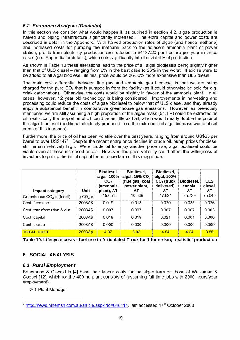
5.2 Economic Analysis (Realistic) In this section we consider what would happen if, as outlined in section 4.2, algae production is halved and piping infrastructure significantly increased. The extra capital and power costs are described in detail in the Appendix. With halved production rates of algae (and hence methane) and increased costs for pumping the methane back to the adjacent ammonia plant or power station, profits from electricity production are reduced to $4187.20 per hectare per year in these cases (see Appendix for details), which cuts significantly into the viability of production.

As shown in Table 10 these alterations lead to the price of all algal biodiesels being slightly higher than that of ULS diesel – ranging from 2% in the best case to 26% in the worst. If excise were to be added to all algal biodiesel, its final price would be 26-50% more expensive than ULS diesel.

The main cost differential between flue gas and ammonia gas biodiesel is that we are being charged for the pure CO2 that is pumped in from the facility (as it could otherwise be sold for e.g. drink carbonation). Otherwise, the costs would be slightly in favour of the ammonia plant. In all cases, however, 12 year old technology is being considered. Improvements in harvesting and processing could reduce the costs of algae biodiesel to below that of ULS diesel, and they already enjoy a substantial benefit in comparative greenhouse gas emissions. However, as previously mentioned we are still assuming a high proportion of the algae mass (51.1%) could be extracted as oil; realistically the proportion of oil could be as little as half, which would nearly double the price of the algal biodiesel (additional electricity produced from the extra non-oil algal biomass would offset some of this increase).

Furthermore, the price of oil has been volatile over the past years, ranging from around US$65 per barrel to over US$1478. Despite the recent sharp price decline in crude oil, pump prices for diesel still remain relatively high. Were crude oil to enjoy another price rise, algal biodiesel could be viable even at these increased prices. However, the price volatility could affect the willingness of investors to put up the initial capital for an algae farm of this magnitude.

Impact category Unit

Biodiesel, algal, 100%

CO2 (ammonia plant), AT

Biodiesel, algal, 15% CO2 (flue gas) coal power plant,

AT

Biodiesel, algal, 100% CO2 (truck delivered),

AT

Biodiesel, canola,

AT

ULS diesel,

AT Greenhouse CO2-e (fossil) g CO2-e -15.654 -10.539 17.621 35.739 75.040

Cost, feedstock 2008A$ 0.019 0.013 0.020 0.035 0.026

Cost, transformation & dist 2008A$ 0.007 0.007 0.007 0.007 0.003

Cost, capital 2008A$ 0.018 0.019 0.021 0.001 0.000

Cost, excise 2008A$ 0.000 0.000 0.000 0.000 0.009

TOTAL COST 2008A¢ 4.37 3.93 4.84 4.24 3.85

Table 10. Lifecycle costs - fuel use in Articulated Truck for 1 tonne-km; ‘realistic’ production

6. SOCIAL ANALYSIS

6.1 Rural Employment Benemann & Oswald in [4] base their labour costs for the algae farm on those of Weissman & Goebel [12], which for the 400 ha plant consists of (assuming full time jobs with 2080 hours/year employment):

1 Plant Manager

8 http://news.ninemsn.com.au/article.aspx?id=648114, last accessed 17th October 2008

20

4 Shift Supervisors

10 Pond Operators

5 Centrifuge Operators

1 Laboratory Manager

2 Laboratory Technicians

However in [4] it is also pointed out that additional employment would be created due to requirements to operate the DAF (dissolved air flotation) screens and extractors, anaerobic digesters and power generation system. However, breakdowns for these jobs are not given. Based on these comments and the additional costs listed, a reasonable estimate would be the additional jobs as follows:

2 Shift Supervisors

5 Digester Operators

2 DAF/Extraction Operators

1 Generator Manager (Electrician)

1 Generator Assistant (Electrician/Mechanic)

In addition to this cost [4] adds “corporate overheads”, which are not listed in any previous study, of about 50%. Presumably in addition to costs for permits and the like this would also include the employment of administrative staff, including general administration, a lawyer, an accountant, a logistics specialist (supply chain), warehouse &distribution operators (store person), drivers and possibly others (whether they be full or part time; probably part time for some). Examination of small businesses suggests these additional jobs would be something along the lines of the following (full time unless otherwise mentioned):

1 Lawyer (part time)

1 Accountant (part time)

1 Logistics Specialist

1 Administrative Assistant

1 Store Manager

1 Store Person

2 Drivers

This results in the original 23 technical staff given in [12], plus another 11 technical and 7 administrative staff (counting the lawyer & accountant as one staff member), for the equivalent of 41 full time jobs all up. Allowing for a bit of variability, this would result in a range of 40-45 people. Increased production rates at the algae farm would lead to some increase in technical staff, but not at a linear rate. It is estimated in [4] that a doubling of algal yields would result in one-third more technical and administrative staff, which would result in 50-60 people. Doubling the size of the algae farm without changing algae production rates would most likely double the number of people employed, so 80-90 staff.

It could be argued that administrative staff would not need to be increased at the same level as technical staff; if this was the case then the lower end figures in the ranges given are likely to be more accurate. However, modern companies typically require more ‘administrative’ staff than previously, e.g. people involved with marketing and advertising the products produced, government lobbyists seeking to obtain excise relief or grants, etc. This could result in additional employment over the jobs listed above.

Given the suggested location of the algae farms in [2], all of the above employment would of a necessity be in rural areas, apart from possibly the part-time Lawyer and Accountant jobs.

21

6.2 Gender analysis All of the employment opportunities listed could be fulfilled equally well by either women or men. As such with a base employment rate of 40-45 people it would be expected that 20-23 women would be employed.

When considering the full cradle-to-grave employment opportunities in algal industries, the present situation is that most algal farms exist to produce products for the health food and nutraceuticals market. If this continues to be the case, for example by extraction of high value products before conversion to biofuel, then there exists the potential for increased female participation in the downstream workforce.

7. CONCLUSIONS

For the designs suggested, greenhouse gas emission and energy balance figures are very favourable for algal biodiesel. At the (relatively) small scale of a single 400 ha algae farm the economics also look to be promising, but if one increases the size to that suitable for a large commercial industry extra costs from increased infrastructure (capital) and power (ongoing) costs could make the biodiesel economically nonviable. Economies of scale do not appear to apply for these types of designs. Furthermore, the proportion of algae biomass that can be extracted as oil could vary greatly; if lower (around 20%) rather than higher (around 50%) figures were achieved in commercial production this would nearly double the cost of the algal biodiesel output.

There is a potential for economic viability at a large scale with improved processing and harvesting techniques; consider that corn ethanol was not viable at a commercial level until the introduction of the molecular sieve in the early 1990s [19].

Given the costs of transporting the biodiesel (generally from a fairly remote location) some distance to an urban area where it is most likely to be used, it is in fact possible that turning all of the algae into electricity could be the best outcome – once the farm is appropriately connected to the grid, there can be an immediate increase in electrical production (given an appropriately sized generator). Increased biodiesel production requires additional transportation to be arranged, with the associated freight costs. The main determinant is whether the focus is on the reduction of greenhouse gas emissions in general, or economic viability; the former may be more important for the owners of coal-fired power stations once the Carbon Pollution Reduction Scheme is enacted; for public affairs relations if not for profit.

Although care has been taken in updating economic figures, extensive validation would be required before considering this design for implementation; consider the numbers as a guide only.

As previously mentioned; we are using Benemann & Oswald’s [4] assumption of 511 kg of algal oil being extractable from 1000 kg of dried algae. For the base case of 109.6 t/ha/yr and 400 ha of ponds (spread over 500 ha of land) that’s 22400 tonnes of oil annually, with 11200 tonnes annually in the ‘realistic’ case. This is equivalent to 44.8 or 22.4 tonnes of oil per hectare of total land area annually, which compares very favourably with palm oil production (3.68 t/ha on average in 2004 in Malaysia according to [21]). Assuming similar biodiesel yields as canola (87.2%) and density (0.88 kg/L) this would yield 22.19 ML of algal biodiesel from 1 algae farm, or 11.09 ML for the ‘realistic’ case, for 44.38 kL/ha/yr and 22.19 kL/ha/yr respectively.

8. ACKNOWLEDGEMENTS

We would like to thank Kurt Liffman, Greg Threlfall and Greg Griffin of CSIRO Materials Science and Engineering for the large amount of work that they have performed in finding and checking many of the references and data that this paper is based upon, Mick Meyer for his help with nitrogen volatilisation, and Tim Grant for his creation of many of the life cycle processes that underlie the LCAs. We would also like to thank Greg Griffin for reviewing the paper.

22

9. REFERENCES 1. Sheehan, J., Dunahay, T., Benemann, J. and Roessler, P. A look back at the U.S

Department of Energy’s aquatic species program: biodiesel from algae, National Renewable Energy Laboratory, Report NREL/TP-580-24190, 1988

2. Regan, D.L. and Gartside, G. Liquid Fuels from Micro-Algae in Australia, CSIRO, Melbourne, Australia, 1983.

3. Hillen, L.W. and Warren, D.R. Hydrocarbon fuels from solar energy via the alga Botryococcus Braunii, Mechanical Engineering Report 148, Aeronautical Research Laboratories, DSTO, 1976.

4. Benemann, J.R. and Oswald, W.J. Systems and economic analysis of microalgae ponds for conversion of CO2 to biomass, Final Report to the Department of Energy, Department of Civil Engineering, University of California Berkeley, 1996

5. Kedem, K.L., Microalgae production from power plant flue gas: Environmental implications on a life cycle basis, Report TP-510-29417, National Renewable Energy Laboratory, Golden, Colorado, 2001.

6. Humphries, R.B., Beer, T. & Young, P.C. Weed Management in the Peel Inlet of Western Australia, in Water and Related Land Resource Systems, ed. Y. Haimes & J. Kindler (Pergamon, Oxford) pp95-103, 1980

7. Spolaore, P., Joannis-Cassan, C., Duran, E. and Isambert, A. Commercial applications of microalgae, J. Bioscience and Bioengineering, 101 (2) 87-96, 2006.

8. Curtain, C. Plant Biotechnology – The growth of Australia’s algal β-carotene industry, Australasian Biotechnology, 10 (3), 19-23, 2000.

9. EPA, WA – Ammonia-Urea Plant, Burrup Peninsula (Dampier Nitrogen Pty Ltd), report and recommendations of the Environmental Protection Authority, Bulletin 1065, Perth, WA, September 2002. Last accessed 8th October 2008 at http://www.epa.wa.gov.au/docs/1373_b1065.pdf

10. Fertilizer Focus, Burrup Fertilisers ammonia plant officially opened, Fertilizer Focus May/June issue, pp. 62-63, 2006. Last accessed 8th October 2008 at http://www.fmb-group.co.uk/downloads/p148-62-63-Burrup.May.pdf

11. Science Education Group, Salters’ Higher Chemistry, University of York, Heinemann Education Publishers, 1999.

12. Weissman, J.C. and Goebel, R.P., Design and Analysis of Pond Systems for the Purpose of Producing Fuels, Solar Energy Research Institute (SERI), Golden, Colorado. Grant number SERI/STR-231-2840, 1987.

13. DuByne, D., The Biogas Revolution, BBI Bioenergy Australasia, October issue, pp. 26-29, 2008.

14. Sazdanoff, N., Modeling and Simulation of the Algae to Biodiesel Fuel Cycle, Honors Undergraduate thesis for College of Engineering, Ohio State University, 2006.

15. Sieg, D., Making Algae Biodiesel At Home, available from www.making-biodiesel-books.com/, Bangkok, Thailand, March 2008.

16. Sheehan, J., Dunahay, T., Benemann, J., Roessler, P., A Look Back at the US Department of Energy’s Aquatic Species Program – Biodesel from Algae, NREL/TP-580-24190, National Renewable Energy Laboratory, Golden, Colarado, July 1998.

17. Benneman, J., Technology Roadmap – Biofixation of CO2 with Microalgae, Final Report (7010000926) to the US Department of Energy, National Energy Technology Laboratory, Morgantown-Pittsburgh, January 14 2003.

23

18. van Harmelen, T., Oonk, H., Microalgae Biofixation Processes: Applications and Potential Contributions to Greenhouse Gas Mitigation Options, TNO Built Environment and Geosciences, Apeldoorn, The Netherlands, May 2006.

19. McAloon, A., Taylor, F., Yee, W., Ibsen, K., Wooley, R., Determining the Cost of Producing Ethanol from Corn Starch and Lignocellulosic Feedstocks, NREL/TP-580-28893, National Energy Technology Laboratory, Golden, Colorado, October 2000.

20. Apelbaum, J., Australian Transport Facts 2001, Apelbaum Consulting Group, Melbourne, Australia, 2003.

21. Sumathi, S., Chai, S.P., Mohamed, A.R., Utilization of oil palm as a source of renewable energy in Malaysia, Renewable and Sustainable Energy Reviews, Volume 12, Issue 9, December 2008, pp. 2404-2421. Online since August 2007 at http://tinyurl.com/6m8cmy

10. APPENDIX OF CALCULATIONS

Several of the values reported in this paper required some calculation to determine. For the reader’s edification these calculations are presented here.

When possible, modern costs for the building, equipment, consumables and labour have been used. When these have been unavailable we have converted US$1994-1996 (as appropriate in [4]) in to A$1994-1996 using the average exchange rate for those years, and then used CPI to convert into A$2008 values. When these were also unavailable we converted A$1983 (as appropriate in [2]) to A$2008 using CPI.

In section 8.4.2 of [4] it is calculated that approximately 1.7 tonnes of supplementary CO2 per tonne of algae is required at an 85% absorption efficiency; so for approximately 109 tonnes of algae per hectare per year 185 tonnes of CO2 are necessary, i.e. 506.5 kg ha-1 day-1. In [2] more optimistic calculations are made requiring only 184 kg ha-1 day-1 (despite only a 50% absorption rate) although adjusting this for a 50% increase in production yields 276 kg ha-1 day-1. The reasoning behind the calculations in [4] appears to be more accurate, so these values are used, which are 83.5% higher than in [2].

In appendix C, section 6 of [2] extensive calculations show that power requirements for pumping flue gas 50 km to the algae farm from a nearby power station requires 29440 kWh per day for 400 ha; applying the aforementioned 83.5% increase but reducing the pipe length to 2.5 km yields 2466.5 kWh per hectare per year. However, operating costs for the flue gas supply power are listed at $1000 per hectare per year with electricity at 6.5 ¢/kWh, indicating 15384.6 kWh per hectare per year are required. It is indicated in [4] that this number is based on a large degree of interpolation; obviously the figures are overstated. Thus, although we use the gas volumes given in [4], we use the power requirements interpolated from [1], which for the ‘base case’ are rounded to 2470 kWh per hectare per year for pumping the flue gas, or 370 kWh per hectare per year for pumping pure CO2 from a nearby ammonia plant (see below).

Whereas in [2] the remaining algal mass (after processing for oil) is fed back into the ponds to provide nutrient recycling, in [4] it is instead moved into an anaerobic digestion unit; basically a covered lagoon. It is predicted in [4] that this would result in 60 tonnes per day (for a 400ha facility) of solids, of which two-thirds would (eventually) be converted into biogas, consisting of about 60% methane and 40% carbon dioxide; i.e. 24 tonnes of methane per day. Pure methane has a heat of combustion of about 891 kJ/mol [11] and a molar mass of 16, so for 1.5 Mmol per day this would be 1336.5 GJ of heat energy9.

9 There are mathematical errors in the calculation for the energy of the methane in [4], including the use of the heat of combustion for natural gas (which is a mix of methane, hydrogen and other gases) rather than pure methane. These have follow-on effects (e.g. the size of the gas-electric generator required) that are taken into account in this paper.

24

At 3600 J/Wh and with a generator (or power station) that is 32% efficient this results in 118.8 MWh of electricity being produced per day (at a rate of 4.95 MW) for the entire algae farm of 400 ha. So for a hectare-year that is 108.48 MWh, which at 8 ¢/kWh is worth $8678.34. For the cases with an adjacent power station or ammonia plant some of this is lost in pumping it back (19.72 MWh/day for the entire algae farm), resulting in a slightly reduced benefit of $8217.40/ha-a.

Power costs for the flue gas case effectively assume that 1.1 million cubic feet per day of gas required for 400 hectares producing 15 g m-2 day-1 are pumped in, so 31150 cubic metres. In the realistic cases only 12 tonnes per day of methane is being produced, rather than 24. Assuming NTP (standard atmospheric pressure and 25 degrees Celsius), 16g of methane occupies 24.5 litres and hence 12 tonnes occupies 18375 cubic metres, so power costs for pumping the methane back will be about 59% of the flue gas pumping costs, or 1896 kWh ha-1 a-1. As mentioned above, 24 tonnes of methane is equivalent to 1336.5 GJ of heat energy, so 12 tonnes is 668.25 GJ.

At a conversion factor into electricity of 32% this results in 59.4 MWh per day for the 400ha algae farm, or 54.2396 MWh ha-1 a-1. Subtracting the cost of pumping the methane back into the power station or ammonia plant yields 52.34 MWh ha-1 a-1 in electrical production, so $4187.20 at 8 ¢/kWh.

Note that conversion efficiencies and the price paid for this electricity could be higher than the conservative values used in this paper, leading to lower prices for algal biodiesel than the figures shown below – e.g. at 12 ¢/kWh flue gas algal biodiesel would cost 3.67 ¢/t-km, making it comparable to ULS diesel at 3.80 ¢/t-km.

Additional inputs are required to transform the dried algae into oil. Lacking any updated information, it is assumed that similar inputs to those required to extract oil from canola are required. In this case, 1 tonne of dried algae will have 1.5 kg of hexane added to it (which if not recovered correctly is then emitted to the air via evaporation), plus energy in the form of steam (1.86 kg, produced from natural gas heating) and electricity (70.18 kWh), to yield 511 kg of algal oil. An additional 3.07 kg of diesel is used in transport, with 3 kg of organic waste produced. The transformation of the algal oil into biodiesel is also assumed to require the same inputs as would be needed for turning canola oil into biodiesel.

In the realistic cases where algae production is halved and piping infrastructure significantly increased, the capital and power costs are increased as follows. When using flue gas, increasing the average distance of algae farm modules from the attached power station to 50 km increases piping/blower costs to 1980A$10550 per hectare with associated power costs of 3214.2 kWh ha-1 a-1. For the ammonia plant case where 100% CO2 is piped to the algae farms the costs are 1980A$1850 ha-1 for the pipes, with ongoing power usage of 482.13 kWh ha-1 a-1, which at 7.5 ¢/kWh is $36.16 per year. Once again based on Macromonitor5, it is possible to determine that in real terms the cost of construction between 1980 and 2008 increased by only 19.2% (less, in fact, than between 1996 and 2008, due to slumps in the 1990s). Thus in 2008A$ the piping and blower capital costs are estimated at $12576 and $2205 per hectare respectively, although these would be expected to increase over the next few years with predicted cost increases in construction and commodities (such as steel and concrete) in general.