
Greenhouse gas emissions related to freshwater...
166
Greenhouse gas emissions related to freshwater reservoirs Guidelines on GHG Measurement Preliminary GHG Assessment Tool Proposal for CDM Methodology Revision January 2010 World Bank Contract 7150219 Supported by Norwegian NTF-PSI THE WORLD BANK
Transcript of Greenhouse gas emissions related to freshwater...

Greenhouse gas emissions related to freshwater reservoirs
Guidelines on GHG Measurement
Preliminary GHG Assessment Tool
Proposal for CDM Methodology Revision
January 2010 World Bank Contract 7150219
Supported by Norwegian NTF-PSI
THE WORLD BANK

Greenhouse gas emissions related to freshwater reservoirs: World Bank Report - January 2010
Page | 2

Greenhouse gas emissions related to freshwater reservoirs: World Bank Report - January 2010
Page | 3
Acknowledgements
This document draws from ongoing research hosted by the International Hydropower Association (IHA), in collaboration with the International Hydrological Programme (IHP) of UNESCO. The collaboration between UNESCO and IHA on this topic is longstanding. Dialogue has been ongoing since the late 1990s. The First International UNESCO/IHA GHG Workshop on the topic was convened in Paris, France, in 2006. Scientific understanding has since been advanced under the UNESCO/IHA GHG Status of Freshwater Reservoirs Research Project (UNESCO/IHA GHG Project), which started in August 2008.
The project has benefited from the collaboration of numerous research institutions and scientists composing the Project’s peer review group (the UNESCO/IHA Forum). This Forum has been established through a series of international workshops, convened over the past three years. The Forum comprises more than 100 institutions, including universities, research institutes, hydropower companies, sponsoring agencies, and others. All documents produced under the UNESCO/IHA GHG Project pass through a peer-review process, being submitted to UNESCO/IHA Forum, before being able to be published in the IHA and UNESCO websites. A key reference established through this scientific community is the Assessment of the “Scoping Paper: GHG Status of Freshwater Reservoirs”, which lead to the initiation of the UNESCO/IHA GHG Project
Further information on the work of the UNESCO/IHA GHG Project can be found at: www.hydropower.org
This document has been proof read by Dr. John Gash.
To all who have contributed to the production of this work, we would like to express our sincere appreciation.
Joel Goldenfum (UNESCO/IHA GHG Research Project Manager) and Richard M. Taylor (IHA Executive Director)
Greenhouse Gas Status of Freshwater
Reservoirs Project

Greenhouse gas emissions related to freshwater reservoirs: World Bank Report - January 2010
Page | 4
Table of Contents
Executive Summary…………………………………………………………………………………………………..….5
Guidelines on GHG Measurement ......................................................11
(Concepts and key parameters)
Preliminary GHG Assessment Tool …………………………………..…….………45
(Decision-tree model to assess GHG vulnerability)
Proposal for CDM Methodology Revision .............................63
(Field measurement and calculation manuals)
Appendices…………………………………………………………………………………………………………………………..….155
Greenhouse gas emissions related to freshwater reservoirs: World Bank Report - January 2010
Page | 5
Executive Summary
Introduction Mitigating climate change has become one of the most important objectives for strategic sustainable development. There is a clear and pressing need to quantify the greenhouse-gas (GHG) footprint of all human activities. The issue of the GHG status of freshwater reservoirs (that is, assessing any change in GHG emissions in a river basin resulting from the creation of a freshwater reservoir) has been raised in both scientific and policy fora.
To quantify any net change of GHG fluxes in a river basin caused by the creation of a reservoir, it is necessary to consider exchanges before and after its construction. This creates a significant problem because there has been no scientific consensus on how to measure the GHG status of freshwater reservoirs.
This lack of agreement has been obstructing progress in decision-making on specific activities. For example, scientific guidance is needed to support the drawing up of national GHG inventories; for methodologies (measurement and predictive modelling) to establish the GHG footprint of new water infrastructure projects; and, to quantify more precisely the carbon offsets of hydropower projects for GHG emission trading. More generally, policy making on energy, water and climate action is compromised by the current lack of understanding. This has a global impact – especially on planning in developing countries.
Despite strong efforts being made to improve the assessment of the GHG status of reservoirs, there are still many uncertainties. Specific problems have been the lack of standard measurement techniques; limited reliable information from different sources; and the lack of standard tools for assessing net GHG exchange from existing and planned reservoirs. Consequently, more research is needed to develop accurate estimates of the GHG impact of freshwater reservoirs.
One consequence resulting from the existing controversy over GHG emissions from freshwater reservoirs is that hydropower projects with reservoirs are currently being subjected to a conservative Clean Development Mechanism (CDM) methodology. The UNFCCC Executive Board has noted that with the current scientific uncertainties, simple criteria, based on a threshold in terms of power density (installed power generation capacity divided by the flooded surface area), is being used to determine the eligibility of
hydropower plants for CDM support. The threshold has no scientific basis and effectively excludes hydropower schemes with significant freshwater reservoirs. (power density less than 4 W/m2) The decision was taken as a precautionary measure, pending further clarification of reports in the scientific literature on GHG emissions associated with such reservoirs. This is but one example of the clear need for a methodology to estimate emissions from reservoirs. Adoption of such a methodology would permit fair evaluation of hydropower projects and enable reservoir projects with low net GHG emissions to qualify for the CDM.
The circumstances described above motivated the International Hydropower Association (IHA) to become involved in dialogue with the scientific community. The UNESCO/IHA GHG Status of Freshwater Reservoirs Research Project (the UNESCO/IHA GHG Project), hosted by IHA in collaboration with the International Hydrological Programme (IHP) of UNESCO, aims to; improve understanding of the impact of reservoirs on natural GHG emissions, obtain a better comprehension of the processes involved, and help to overcome knowledge gaps.
Following several years of preliminary work, the UNESCO/IHA GHG Project started in August 2008. The objectives and outlines of the project were set by two scientific workshops hosted by UNESCO (in 2006, in Paris, France and in 2007, in Foz do Iguaçu, Brazil), as part of UNESCO IHP-VI 2002-2007 work programme. These events were followed by a meeting in Paris in January 2008 which finalised the state-of-the-art paper “Scoping Paper: GHG Status of Freshwater Reservoirs” by Tucci, C., et al., UNESCO/IHA; April 2008.
The main objectives of the UNESCO/IHA GHG Project are to:
• develop, through a consensus-based, scientific approach, detailed measurement guidance for net GHG assessment; promote scientifically rigorous field measurement campaigns, and the evaluation of net emissions from a representative set of freshwater reservoirs throughout the world;
• build a standardised, credible set of data from these representative reservoirs;
• develop predictive modelling tools to assess the GHG status of unmonitored reservoirs and potential sites for new reservoirs; and
• develop guidance and assessment tools for mitigation of GHG emissions for sites vulnerable to high net emissions.
Greenhouse gas emissions related to freshwater reservoirs: World Bank Report - January 2010
Page | 6
The project has indeed benefitted from a consensus-based, scientific approach, with intensive international coverage, involving the collaboration of numerous institutions. All deliverables are reviewed by the Project’s peer review group (UNESCO/IHA Forum, composed of researchers, scientists and professionals from more than 100 institutions.
As part of the effort to move these initiatives forward, IHA has been in contact with the World Bank, which shares many of the concerns outlined above. This led to the current assignment under the World Bank Contract (Ref 7150219), with the following deliverables:
1. Guidelines for GHG measurements: it is important that estimates should be based on data collected with a consistent protocol, underpinned by a sound understanding of the science involved in GHG emissions. The concepts and key parameters for such a methodology are presented here, with a specific field measurement protocol included in the third component of this document.
2. A preliminary GHG assessment tool: a simple decision-tree model is presented for analysis of GHG emissions from freshwater reservoirs. This classifies a reservoir as having “low”, “medium” or “high” vulnerability to gross GHG emissions.
3. Proposal for CDM methodology revision: a specific field measurement protocol is put forward, together with a preliminary version of a calculation manual. This is proposed as a basis for hydropower methodology revision in the Clean Development Mechanism (CDM), with the objective of ensuring a fair, scientifically sound treatment of storage hydropower as a development option under CDM.
A glossary is also included.
The potential users of the products are water-quality specialists, project developers, reservoir owners/operators and government regulators. Clearly, further development will be required to enhance this work, and the World Bank is requested to assist in the necessary funding of this moving forwards.
Additional background information on the UNESCO/IHA GHG Project is provided in Appendix 2.
Summary of Individual deliverables
Deliverable 1: Guidelines for net GHG measurements This guidance is aiming at international standardisation and objective measurements that will ease comparison, transferability and global use of data.
The objective of this deliverable (the Guidelines) is to provide guidelines for international standardised measurement procedures to assess net GHG emissions from man-made freshwater reservoirs (the GHG impact from the creation of freshwater reservoirs), aiming to ensure objective assessments. The Guidelines are applicable to all types of climate and different reservoir conditions, presenting the main concepts and description of processes involved in performing these measurements, including:
General principles and data:
Introduction to the inland waters component of the carbon cycle and to the generally available data. Description of previous work. Introduction to the main principles for taking GHG measurements from reservoirs, including key processes and parameters, stressing the importance of considering net emissions, with the need for pre- and post-impoundment assessments, including the role of carbon and nutrient loading from the catchment, from natural and unrelated human activities.
Spatial and temporal resolution
How seasonal changes in climate, reservoir operations and carbon load may impact the temporal resolution. Recommendations on where and when to measure, including considerations of vegetation and land use (pre- and post-impoundment), hydrological and water-quality issues, other anthropogenic activities and practical issues like accessibility, safety and other indirect implications that should be included when designing the spatial resolution.
Methods and equipment
What to measure, how to measure and general description of the main equipment, for measuring carbon (carbon cycle), GHG emissions, carbon storage in sediments, and physical and water-quality parameters, highlighting advantages and constraints. Detailed descriptions of the

Greenhouse gas emissions related to freshwater reservoirs: World Bank Report - January 2010
Page | 7
procedures and recommended equipment are presented in the Field Manual (see Deliverable 3a).
Data analysis
Main concepts on how to calculate net emissions resulting from the creation of a reservoir in a river basin. Detailed guidance for calculations and extrapolations, comparison of different methodologies, uncertainty, quality assurance and quality control are provided in the Calculation Manual (see Deliverable 3b).
It is stressed that these Guidelines are intended to be a living and dynamic document, to be regularly updated. This will be achieved through the ongoing UNESCO/IHA GHG Project.
Deliverable 2: Preliminary GHG Assessment Tool Present scientific knowledge does not allow the development of a model capable of directly estimating net GHG emissions (i.e., the GHG impact from the creation of a freshwater reservoir). This deliverable is therefore developed as a Risk Assessment Tool for Reservoir Vulnerability to Gross GHG Emissions (referred to here as the Risk Assessment Tool). It is intended to provide a first estimate of the likelihood of existing or future reservoirs to have high gross GHG emissions, as a first step towards the evaluation of the net GHG emissions. The identification of high vulnerability to gross GHG emissions should be taken as a warning of the need for further studies on the site, with detailed field monitoring to determine the net GHG emissions of the reservoir.
The Risk Assessment Tool is a first, simple model targeted at project developers, reservoir owners or government agencies, to allow a quick assessment of a potential site and to assess its vulnerability to gross GHG emissions, in the absence of site-specific measurement data. It can also be applied as a tool for designing reservoir field campaigns, with a view to sampling representative reservoirs for data input into further development of predictive models.
Due to the high level of uncertainty observed in the available data, the Risk Assessment Tool described here is presented as a prototype — a first example of a simple model. It was developed on the basis of theoretical knowledge obtained from the available information on key parameters and processes.
The Risk Assessment Tool applies a decision-tree system to allow the relatively quick assessment of the vulnerability of a reservoir to gross GHG emissions as “low”, “medium” or “high”, using information obtained from key variables, such as: carbon and nutrient load, water temperature, wind speed and direction, rainfall, soil type, land use, and reservoir characteristics (residence time, presence of low level outlets, stratification of the reservoir body, reservoir shape, water depth, reservoir age, drawdown zone exposure, and biomass in the reservoir and in the drawdown zone).
As this analysis is based on information from key parameters (e.g. residence time, water temperature, biomass, and others), it is important to define “high,” “medium” and “low” levels not only for the GHG emissions, but also for these parameters. As the available data still do not allow a proper estimation of these limits, the analysis has been done in a qualitative way. When more information becomes available, future versions of this document can include more precise definitions of the levels for the key parameters.
Decision trees to assess the vulnerability of reservoir sites to gross methane (CH4) and nitrous oxide (N2O) emissions are presented as the main elements in assessing the risks of GHG emissions. The vulnerability of a site to carbon dioxide (CO2) emission is not included in the model because CO2 emissions are potentially similar at the basin level, for pre- and post-impoundment conditions, although they may be influenced in time and space by the creation of a reservoir.
It is important to stress that the results from the present study have to be interpreted with caution, as the complexity of the processes and limitations in the data result in substantial uncertainties. As more information becomes available, and more indicators are included, the risk assessment tool will be improved. It will be updated as experience is gained in its application and the needs of users.
Deliverable 3: Proposal for CDM Methodology Revision The CDM Executive Board has ruled that reservoir storage hydropower projects must meet specified power density thresholds. At present, the criterion is that hydropower projects with power densities less than or equal to 4 W/m2 cannot receive CDM support. This criterion effectively excludes reservoir storage hydropower from the CDM. An exception to this is any project that can

Greenhouse gas emissions related to freshwater reservoirs: World Bank Report - January 2010
Page | 8
demonstrate through specific measurement GHG emissions from the reservoir would be of a relatively low level.
The Field Manual and the Calculation Manual were developed based on the concepts presented in the Guidelines presented in Deliverable 1. These manuals describe what, when, where and how to measure the relevant key parameters, and how to estimate the net GHG emissions (the GHG impact from the creation of freshwater reservoirs) from these measurements.
The Field Manual and the Calculation Manual are proposed as the basis for a CDM approach in a revised “Approved Consolidated Methodology 002” (ACM002) or a “new methodology”. It is proposed that these manuals should provide the means to directly measure and calculate net GHG emissions of reservoir storage hydropower projects currently excluded from the CDM.
This proposed methodology would allow a clear approach to calculating emissions from reservoirs and will include options for a standardised approach to measurement and calculation in the face of natural variability and data uncertainty. It will enable reservoir hydropower projects with low net GHG emissions to qualify for potential admission to the CDM.
Part A: Field Manual
The Field Manual provides instructions on the field methods and equipment necessary to estimate GHG emissions, under pre- and post-impoundment conditions. It gives qualified technicians and scientists a protocol to make GHG emission measurements in the field. More specifically, the Field Manual includes instructions on how to conduct GHG measurements in terrestrial (forest, grass and peatland) and aquatic (wetland, lake, river and reservoir) ecosystems in terms of GHG emissions and carbon and nitrogen stocks.
This volume is a first complete version of the Field Manual. It is considered a draft version because it has not yet been submitted to the UNESCO/IHA peer-review process, which may introduce further enhancement. As with the other volumes, it will be regularly updated, through the ongoing UNESCO/IHA GHG Research Project.
Part B: Calculation Manual
The Calculation Manual presents the standard procedures that are needed to calculate net GHG emissions resulting from the creation of a reservoir in a river basin. This manual is designed to be used
with the data obtained from the procedures described in the companion Field Manual.
As the Calculation Manual is in an early draft stage, the document provided constitutes a framework and annotated list of contents, describing the proposed format, objectives, elements to be considered, and general structure. More research is needed to complete this document so that it can constitute a valuable element for the development of a new methodology for reservoir storage hydropower for the CDM. Further refinement will be progressed through the UNESCO/IHA GHG Project.
Next steps The initiatives of the UNESCO/IHA GHG Project constitute a pioneering step for the standardisation of equipment and procedures for an accurate evaluation of the net GHG impact of freshwater reservoirs. These protocols can fill the need for standard procedures, as they were developed through a consensus-based approach, and are ready for application in a range of reservoirs, helping to obtain representative, comparable and transferable data, and thus allowing scientifically sound evaluation of the ‘GHG footprint’.
The project is reaching a stage where the Measurement Guidance is available; several IHA members have indicated willingness to conduct field measurement campaigns. The next step is to identify additional parties with reservoir sites to complete a reasonable spectrum of reservoir types and geographic locations.
As the UNESCO/IHA GHG Project has progressed, the need to develop a capacity-building programme has been identified, particularly in the context of the developing world. This programme would raise awareness on estimating the GHG risk from reservoir projects, as well as specific measurement training. Such training would ensure a proper understanding and application of the standard procedures developed under the UNESCO/IHA GHG Project.
Next, it will be necessary to ensure that the knowledge obtained from the application of the proposed procedures can be applied to the development of adequate predictive modelling tools to assess the GHG status of unmonitored reservoirs and potential sites for new reservoirs. These tools, once validated, can be the basis for

Greenhouse gas emissions related to freshwater reservoirs: World Bank Report - January 2010
Page | 9
developing appropriate guidance on national GHG inventories and to quantify carbon offsets for emission trading, without the need for specific field measurement campaigns.
The next steps will require funding to meet the need for:
• Completion of the Field Manual and the Calculation Manual;
• Promotion of field measuring campaigns in compliance with the proposed methodology;
• Capacity-building programmes for such field measurements;
• Development of predictive modelling tools to assess the GHG status of unmonitored reservoirs and potential new reservoir sites;
• Development of guidance for mitigation of GHG emissions at vulnerable sites.
It is essential to continue the role of the UNESCO/IHA Forum, including participation in workshops and the peer-review process. This is a time- and resource-intensive process, which is
largely undertaken voluntarily. This could be managed through the support of an independent scientific and stakeholder advisory panel to ensure participation in the Project. This would contribute to reinforcing the strong, transparent, consistent and ongoing peer-review process that the Project requires.
The Field Manual and the Calculation Manual are likely to have to be repackaged to fit CDM requirements for requesting a revision to an existing (or creating a new) monitoring methodology. Time, cost, and availability of a 'vehicle' reservoir hydropower project will determine the route taken. A successful result would enable reservoir hydropower projects to fully participate in the CDM.

Greenhouse gas emissions related to freshwater reservoirs: World Bank Report - January 2010
Page | 10

Greenhouse gas emissions related to freshwater reservoirs: World Bank Report - January 2010
Page | 11
Deliverable 1
Guidelines on GHG Measurement
Version 1 – January 2010

Greenhouse gas emissions related to freshwater reservoirs: World Bank Report - January 2010
Page | 12
Acknowledgements This deliverable was developed under the UNESCO/IHA Project – GHG Status of Freshwater Reservoirs Research Project (the UNESCO/IHA GHG Research Project), hosted by the International Hydropower Association (IHA), in collaboration with the International Hydrological Programme (IHP) of UNESCO and benefitted from the collaboration of numerous research institutions and scientists composing the UNESCO/IHA GHG Research Project Peer Review Group (the UNESCO/IHA Forum).
We would like to express our sincere appreciation of the work carried out by all experts who took part in the UNESCO/IHA Workshops, and acknowledge the very large number of constructive comments received.
Particularly, we would like to acknowledge the following experts, for their collaboration to this specific document:
Document track:
Drafted by: Joel A. Goldenfum
Comments from members of the Panel of Experts (Field Measurement): Assiran Assireu, Stéphane Descloux, Miguel F Doria, Michael Fink, Jon Guðmundsson, Frédéric Guérin, Atle Harby, Yves Prairie, Fábio Roland, Marco Aurélio dos Santos, Håkon Sundt, Richard Taylor, Alain Tremblay.
Comments from members of the UNESCO/IHA Peer Review Group: Gwenaël Abril, Jason Antenucci, Julie Bastien, Vincent Chanudet, Philip Fearnside, Robert Gill, Clelia Marti, John Melack, International Rivers, Elizabeth Sikar.
Scientific proof reading: Dr. John Gash.

Greenhouse gas emissions related to freshwater reservoirs: World Bank Report - January 2010
Page | 13
Summary
World Bank Contract 7150219
Deliverable 1: Guidelines on GHG Measurement
This document was developed by the International Hydropower Association (IHA) under the World Bank Contract 7150219, to fulfil the requirements of Deliverable 1 of the contract terms: Guidelines for net GHG measurements aiming at international standardisation and objective measurements that will ease comparison, transferability and global use of data.
The objective of this document (the Guidelines) is to provide guidelines for internationally standardised measurement procedures to assess net GHG emissions from man-made freshwater reservoirs (the GHG impact from the creation of freshwater reservoirs), aiming to ensure objective assessments and to ease comparison, transferability and the global use of data. The Guidelines are applicable to all types of climate and different reservoir conditions, presenting the main concepts and description of processes involved in performing these measurements, including:
General principles and data: Introduction to the inland waters component of the carbon cycle and to the generally available data. Description of previous work. Introduction to the main principles, including key processes and parameters, stressing the importance of considering net emissions, with the need for pre- and post-impoundment assessments, including the role of carbon and nutrient loading from the catchment, from natural and unrelated human activities.
Spatial and temporal resolution: How seasonal changes in climate, hydro-operations and carbon load may impact the temporal resolution. Recommendations on where and when to measure, including considerations of vegetation and land use (pre- and post-impoundment), hydrological and water quality issues, other anthropogenic activities and practical issues like accessibility, safety and other indirect implications that should be included when designing the spatial resolution.
Methods and equipment: What to measure, how to measure and general description of the main equipment, for measuring carbon (carbon cycle), GHG emissions, carbon storage in sediments, and physical and water-quality parameters, highlighting advantages and constraints. Detailed descriptions of the procedures and recommended equipment are presented in the Field Manual.
Data analysis: Main concepts on how to calculate net emission resulting from the creation of a reservoir in a river basin. Detailed guidance for calculations and extrapolations, comparison of different methodologies, uncertainty, quality assurance and quality control are provided in the Calculation Manual.
It is stressed that these Guidelines are intended to be a living and dynamic document, to be regularly updated. This will be achieved through the ongoing UNESCO/IHA GHG Research Project

Greenhouse gas emissions related to freshwater reservoirs: World Bank Report - January 2010
Page | 14
Table of contents
I. Introduction ............................................................................................................... 16
I.1. Background ......................................................................................................................... 16
I.2. Objective and Applicability of the Guidelines ..................................................................... 16
II. General principles and data .............................................................. 17
II.1. Previous Work ..................................................................................................................... 17
II.2. Key Processes and Parameters ........................................................................................... 19
II.2.1. Carbon Cycle in a Natural Catchment ................................................................... 19
II.2.2. Pathways in Reservoirs ......................................................................................... 20
II.2.3. N2O - Main Processes and Pathways .................................................................... 21
II.2.4. Key Processes ........................................................................................................ 21
II.2.5. Key Parameters ..................................................................................................... 22
II.3. The Importance of Considering Net Emissions ................................................................... 22
II.3.1. Definition of Net Emissions ................................................................................... 22
II.3.2. Measurement of Gross Emissions ........................................................................ 23
II.3.3. Change in Storage in the Reservoir ....................................................................... 23
II.3.4. Output from the Reservoir ................................................................................... 23
II.3.5. Pre-Impoundment Measurements ....................................................................... 24
II.3.5.1. Catchment/Reservoir - Terrestrial ................................................................ 25
II.3.5.2. Catchment/Reservoir - Aquatic .................................................................... 25
II.3.5.3. Downstream of the Reservoir Site ............................................................... 25
II.3.5.4. Assessment of Carbon Stock ........................................................................ 25
II.3.6. Post-Impoundment Measurements ..................................................................... 26
II.3.6.1. Catchment .................................................................................................... 26
II.3.6.2. In the Reservoir ............................................................................................ 26
II.3.6.3. Downstream of the Reservoir Site ............................................................... 26
II.4. Standardisation of Units ..................................................................................................... 26
III. Spatial and temporal variability .................................................. 26
III.1. Where to Measure .............................................................................................................. 27
III.2. When to Measure ............................................................................................................... 28
IV. Methods and equipment ..................................................................... 29
IV.1. Procedures for Measuring GHG Emissions ......................................................................... 29
IV.1.1. Terrestrial Systems ............................................................................................... 29

Greenhouse gas emissions related to freshwater reservoirs: World Bank Report - January 2010
Page | 15
a. Chambers .......................................................................................... 29
b. Incubators (Soil Core Sampling) ........................................................ 30
c. Eddy Covariance Towers ................................................................... 30
Other Alternatives to Estimate Emissions ............................................................ 31
IV.1.2. Aquatic Systems .................................................................................................... 31
IV.1.2.1. Diffusive Surface Flux Between Water and the Atmosphere ....................... 31
a. Surface Floating Chambers ............................................................... 31
b. Eddy Covariance Towers ................................................................... 32
c. Thin Boundary Layer (TBL) Diffusive Process Model ......................... 32
IV.1.2.2. Bubbling (or Ebullition) ................................................................................. 33
IV.1.2.3. Downstream Emissions ................................................................................ 34
IV.1.2.3.1. Degassing .......................................................................................... 34
IV.1.2.3.2. Downstream Diffusive Fluxes ............................................................ 35
IV.1.2.4. CO2, CH4 and N2O Concentrations ................................................................ 35
IV.2. Carbon Mass Flow and Carbon Storage in Sediments ........................................................ 36
IV.3. Water Quality and Physical Parameters ............................................................................. 36
V. Data analysis ............................................................................................................. 37
VI. Updating these guidelines ................................................................... 38
VII. References ................................................................................................................... 39

Greenhouse gas emissions related to freshwater reservoirs: World Bank Report - January 2010
Page | 16
I. Introduction
I.1. Background The scoping paper “Assessment of the GHG status of Freshwater Reservoirs” (Tucci, C., et al., 2008) has been used as a key reference in the drafting of this document as it is considered to represent the state of the art on this subject.
According to UNESCO/IHA (2008), freshwater reservoirs are used to regulate flow for many purposes, including: water supply, irrigation, flood mitigation, drought protection, navigation and hydropower. Flux measurements above the water surfaces of flooded land have indicated that changes in the emission of carbon dioxide, methane and nitrous oxide may occur at levels that are relevant to inventories of greenhouse gas (GHG) exchanges. Research suggests that emission levels in cold and temperate climates are generally low, but that high emissions may be observed in some tropical systems with persistent anoxia (e.g., Tremblay et al. 2005). However, it is important to improve the available information about the GHG status of existing and new reservoirs and provide the tools needed to support sound decision making on the mitigation measures that may be necessary.
To quantify the net change of GHG exchange in a river basin caused by the creation of a reservoir, it is necessary to consider exchanges before, during and after the construction of the reservoir. The difference between pre- and post-reservoir emissions from the portion of the river basin influenced by the reservoir will indicate the net GHG emissions of the reservoir. In accordance with IPCC (2006), the lifecycle assessment period for net GHG emissions is 100 years. For the purpose of this document, net lifecycle GHG emissions is taken as a proxy for the carbon footprint of the reservoir.
Limited published data from tropical reservoirs indicates that GHG emissions vary not only among reservoirs, but also within each reservoir. This variation may have many causes, including: carbon/nutrient loading from the catchment; temperature; oxygen concentration; type and density of the flooded vegetation; aquatic flora and fauna; residence time; wind speed; thermal structure; reservoir topography and shape; and water level.
I.2. Objective and Applicability of the Guidelines The objective of these Guidelines for net GHG measurements aiming at international standardisation and objective measurements that will ease comparison, transferability and global use of data (the Guidelines) is to provide guidance for standardised measurements to assess net GHG emissions associated with reservoirs1
The Guidelines are to be used to plan and conduct measurement campaigns to estimate net GHG emissions from freshwater reservoirs before and after their construction, aiming to ensure objective assessments and to ease comparison, transferability and the global use of data (subject to rules of access). It aims to promote scientifically sound evaluation of the GHG exchange due to the construction of a freshwater reservoir.
.
Since 2008, UNESCO and the International Hydropower Association have been hosting an international research project, which aims to improve understanding on the impact of reservoirs on natural GHG emissions, obtaining a better comprehension on the processes involved and helping to overcome knowledge gaps. The overall objective of the Project is to allow the evaluation of the carbon footprint (net GHG emissions), due to the construction of a freshwater reservoir within a river basin, as well as the identification of potential mitigation measures. The Project thus aims to: develop, through a consensus-based, scientific approach, detailed measurement guidance for net GHG assessment; promote scientifically rigourous field measurement campaigns, evaluating net emissions from a representative set of freshwater reservoirs throughout the world; build a standardised, credible set of data from these representative reservoirs; develop predictive modelling tools to assess the GHG status of unmonitored reservoirs and potential new reservoir sites; and develop guidance and assessment tools for mitigation of GHG emissions for vulnerable sites.
1 The term “reservoir” is understood as defined in the UNESCO/WMO International Glossary of Hydrology (1992): “body of water, either natural or man-made, used for storage, regulation and control of water resources”. This glossary is the result of a comprehensive worldwide consultation of hydrological experts. There is no global consensus that “reservoirs” are necessarily man-made and, for this reason, the expression “man-made” is included in the present document.

Greenhouse gas emissions related to freshwater reservoirs: World Bank Report - January 2010
Page | 17
As part of the UNESCO/IHA GHG Research Project, it is intended that these Guidelines will be utilised to assess GHG emissions in a sample of representative sites worldwide. Data produced from this initiative will assist in improving predictive capacity on this issue. For vulnerable sites potential mitigation measures can be developed in the future.
These Guidelines are to be applicable world-wide, for all types of climate and different reservoir conditions, and for reservoirs of all types and purposes. There are several different purposes of freshwater reservoirs, but the GHG-related processes are similar irrespective of the purpose. An additional aspect is reservoirs which have low level outlets (such as turbines, gates and valves) that can exhibit the GHG pathway referred to as degassing (see Section II).
Measurements should include all three of the identified GHG species:
• Carbon dioxide (CO2) - According to the European Environmental Agency (EEA), CO2 emissions account for the largest share of GHGs (equivalent to 80-85% of the emissions).
• Methane (CH4) - Emissions are of importance, because reservoirs may create the conditions under which CH4 can be produced and the global warming potential of CH4 is 21 times stronger than CO2 (UNFCCC, 100 year time horizon).
• Nitrous oxide (N2O) - There is insufficient knowledge on N2O emissions to evaluate their importance; however it should be noted that the global warming potential of N2O is 310 stronger than CO2 (UNFCCC, 100 year time horizon).
An important issue is the identification of key processes and parameters. Determining the relative importance of the different processes helps to identify the main drivers of GHG emissions from reservoirs. Then attention can be focused on the measurements of processes that effectively control the emissions. UNESCO/IHA (2008) identified key aspects of significant GHG emissions. However, their importance has to be tested under a comprehensive field measurement programme, as proposed in these Guidelines. At the end of this measurement programme, the available data may justify a two tier approach in the future:
• [1] assessments of key parameters to check if there are likely to be significant emissions;
• [2] if so, more intensive monitoring to quantify the net GHG emissions.
These Guidelines are being developed as a ‘living document’. As further experience is gained, and uncertainties are reduced, these Guidelines will be updated and future versions will include newly available information.
II. General principles and data The main issues on the contribution, or potential contribution, of reservoirs as sources of GHG are the following:
• What is the GHG status of the river basin before reservoir impoundment?
• What is the observed range of fluxes of the major GHGs to and from the reservoir and the portion of river basin influenced by the reservoir?
• What is the observed storage of carbon in the accumulating sediments and the net primary production of the reservoir and the portion of river basin influenced by the reservoir?
• What fraction of GHG fluxes and carbon storage is a result of the construction of the reservoir?
• If necessary, is it possible to reduce (mitigate) emissions from reservoirs, including future projects?
The following sections present an introduction to the inland waters component of the carbon cycle and to the generally available data, including the main principles, highlighting the existence of several different approaches and stressing the importance of considering net emissions, with the need for pre- and post-impoundment assessments, and the role of carbon and nutrient loading from the catchment, from natural and human activities.
II.1. Previous Work Cole et al. (2007) estimate that inland waters annually receive, from a combination of background and anthropogenically altered sources, on the order of 1.9 Pg C/year from the terrestrial landscape. Of this about 0.2 Pg C/year is buried in aquatic sediments, at least 0.8 (possibly much more) is returned to the atmosphere as gas exchange, while the remaining 0.9 Pg C/year is delivered to the oceans. Clearly, freshwater
Greenhouse gas emissions related to freshwater reservoirs: World Bank Report - January 2010
Page | 18
systems play a fundamental role in the natural carbon cycle.
In the last decade, freshwater reservoirs have been investigated as potential sources of CO2 and CH4 emissions to the atmosphere, in boreal (Rudd et al., 1993; Duchemin et al., 1995; Kelly et al., 1997; Huttunen et al., 2002; Tremblay et al. 2005), temperate (Therrien et al. 2005; Soumis et al., 2004, Casper et al. 2000) and tropical (Keller and Stallard, 1994; Rosa and Schaeffer, 1994; Galy-Lacaux et al., 1997, 1999; Delmas et al., 2001; Rosa et al., 2003; Abril et al., 2005; Sikar et al. 2005; Santos et al., 2006; Guerin et al. 2006; Kemenes et al. 2007) regions. GHG emissions from reservoirs at the global scale are subject to large uncertainties, and there is an urgent need for more observations and a better understanding of the processes involved. Simulation models are likely to play an important role in understanding and analysing the changes in GHG emissions that may occur due to the construction of a reservoir in a river basin (UNESCO/IHA, 2008).
Limited work has been conducted to estimate the significance of the net CO2 balance of aquatic ecosystems compared to the CO2 balance of terrestrial ecosystems at the basin scale. In some temperate and tropical catchments, CO2 emissions from the aquatic ecosystems have been shown to be close to balancing the CO2 uptake by the surrounding forest (Cole and Caraco, 2001; Richey et al., 2002).
Flux measurements at the water-atmosphere or land-atmosphere interface are often the only type of measurements reported in the literature. Few measurements of material transported into or out of the reservoir have been reported, and few
studies have quantified carbon accumulation in reservoir sediments (UNESCO/IHA, 2008).
Age of the reservoir is an important issue. Younger reservoirs in the first years after impoundment need more measurements to capture the changes in emission rates and carbon stocks as the system adjusts. In boreal and temperate conditions GHG emissions have been observed to return to natural levels in less than ten years after impoundment (Tremblay, 2008). Further measurements (as proposed in this document) should reveal how quickly new reservoirs reach equilibrium under tropical conditions.
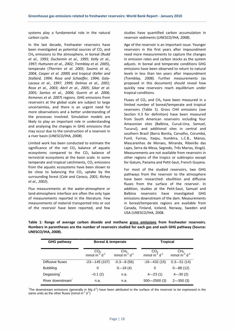
Fluxes of CO2 and CH4 have been measured in a limited number of boreal/temperate and tropical reservoirs (Table 1). Gross CH4 emissions (see Section II.3 for definition) have been measured from South American reservoirs including four Amazonian sites (Balbina, Curuá-Una, Samuel, Tucuruí), and additional sites in central and southern Brazil (Barra Bonita, Carvalho, Corumbá, Funil, Furnas, Itaipu, Itumbira, L.C.B., Manso, Mascarenhas de Moraes, Miranda, Ribeirão das Lajes, Serra da Mesa, Segredo, Três Marias, Xingó). Measurements are not available from reservoirs in other regions of the tropics or subtropics except for Gatum, Panama and Petit-Saut, French Guyana.
For most of the studied reservoirs, two GHG pathways from the reservoir to the atmosphere have been researched: ebullition and diffusive fluxes from the surface of the reservoir. In addition, studies at the Petit-Saut, Samuel and Balbina reservoirs have investigated GHG emissions downstream of the dam. Measurements in boreal/temperate regions are available from Canada, Finland, Iceland, Norway, Sweden and USA (UNESCO/IHA, 2008.
Table 1: Range of average carbon dioxide and methane gross emissions from freshwater reservoirs. Numbers in parentheses are the number of reservoirs studied for each gas and each GHG pathway (Source: UNESCO/IHA, 2008).
GHG pathway Boreal & temperate Tropical
CO2 CH4 CO2 CH4
mmol m-2 d-1 mmol m-2 d-1 mmol m-2 d-1 mmol m-2 d-1
Diffusive fluxes -23—145 (107) -0.3—8 (56) -19—432 (15) 0.3—51 (14)
Bubbling 0 0—18 (4) 0 0—88 (12)
Degassing* ∼0.1 (2) n.a. 4—23 (1) 4—30 (2)
River downstream* n.a. n.a. 500—2500 (3) 2—350 (3)
*The downstream emissions (generally in Mg d-1) have been attributed to the surface of the reservoir to be expressed in the same units as the other fluxes (mmol m-2 d-1)
Greenhouse gas emissions related to freshwater reservoirs: World Bank Report - January 2010
Page | 19
II.2. Key Processes and Parameters The identification of key processes and parameters leads to a better understanding of the mechanisms controlling GHG emissions associated with reservoirs. The following sections describe the key aspects of significant GHG emissions (UNESCO/IHA, 2008).
II.2.1. Carbon Cycle in a Natural Catchment
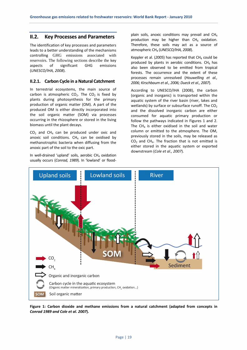
In terrestrial ecosystems, the main source of carbon is atmospheric CO2. The CO2 is fixed by plants during photosynthesis for the primary production of organic matter (OM). A part of the produced OM is either directly incorporated into the soil organic matter (SOM) via processes occurring in the rhizosphere or stored in the living biomass until the plant decays.
CO2 and CH4 can be produced under oxic and anoxic soil conditions. CH4 can be oxidised by methanotrophic bacteria when diffusing from the anoxic part of the soil to the oxic part.
In well-drained ‘upland’ soils, aerobic CH4 oxidation usually occurs (Conrad, 1989). In ‘lowland’ or flood-
plain soils, anoxic conditions may prevail and CH4 production may be higher than CH4 oxidation. Therefore, these soils may act as a source of atmospheric CH4 (UNESCO/IHA, 2008).
Keppler et al. (2005) has reported that CH4 could be produced by plants in aerobic conditions. CH4 has also been observed to be emitted from tropical forests. The occurrence and the extent of these processes remain unresolved (Houwelling et al., 2006; Kirschbaum et al., 2006; Dueck et al., 2007).
According to UNESCO/IHA (2008), the carbon (organic and inorganic) is transported within the aquatic system of the river basin (river, lakes and wetlands) by surface or subsurface runoff. The CO2 and the dissolved inorganic carbon are either consumed for aquatic primary production or follow the pathways indicated in Figures 1 and 2. The CH4 is either oxidised in the soil and water column or emitted to the atmosphere. The OM, previously stored in the soils, may be released as CO2 and CH4. The fraction that is not emitted is either stored in the aquatic system or exported downstream (Cole et al., 2007).
Figure 1: Carbon dioxide and methane emissions from a natural catchment (adapted from concepts in Conrad 1989 and Cole et al. 2007).

Greenhouse gas emissions related to freshwater reservoirs: World Bank Report - January 2010
Page | 20
Figure 2: General concept for all units in a GHG emission study (UNESCO/IHA, 2008)
II.2.2. Pathways in Reservoirs
According to UNESCO/IHA (2008), the source of carbon for the CO2 and CH4 is derived from:
• OM imported from the catchment; • OM produced in the reservoir; • decomposition of OM in plants and soils
flooded by the reservoir.
CO2 is produced in oxic and anoxic conditions in the water column, and in the flooded soils and sediments of the reservoir and is consumed by aquatic primary producers in the euphotic zone of the reservoir. CH4 is produced under anaerobic
conditions, primarily in the sediments; a portion will be oxidised to CO2 by methanotrophic bacteria in the water and sediments under aerobic conditions (Figure 3). Pathways for CH4 and CO2
emissions to the atmosphere from reservoirs include: (1) bubble fluxes (ebullition) from the shallow water; (2) diffusive fluxes from the water surface of the reservoir; (3) diffusion through plant stems; (4) degassing just downstream of the reservoir outlet(s); and (5) increased diffusive fluxes along the river course downstream (Figure 3).
Figure 3: Carbon dioxide and methane pathways in a freshwater reservoir with an anoxic hypolimnion. For reservoirs with a well-oxygenated water column, methane emissions through pathways (2), (4) and (5) are reduced.
Greenhouse gas emissions related to freshwater reservoirs: World Bank Report - January 2010
Page | 21
II.2.3. N2O-Main Processes and Pathways
N2O is produced by both natural processes and human-related activities. Primary human-related sources of N2O are agricultural soil management, animal-manure management, sewage treatment, mobile and stationary combustion of fossil fuel, adipic acid production and nitric acid production. N2O is also produced naturally from a wide variety of biological sources in soil and water, particularly microbial action in wet tropical forests (USEPA, 2009).
N2O is produced in soils by both nitrification and denitrification reactions. Nitrification is an aerobic microbial process that converts ammonium (NH4
+) to nitrate (NO3
-) in the presence of oxygen. During denitrification, nitrates are transformed into nitrogen (N2). Denitrification requires anoxic conditions, but denitrifying bacteria are facultative anaerobes (Schlesinger, 1997; Hahn et al., 2000).
The higher N2O emission from tropical conditions could reflect the influence of temperature on nitrification and denitrification reactions, as well as nitrogen availability, which is greater in tropical than in boreal and temperate forests (Sitaula and Bakken, 1993; Stange et al., 2000; Clein et al., 2002).
There are still significant uncertainties about the contribution of the individual sources to atmospheric N2O. Aquatic systems are considered to be significant, but not the dominant sources of atmospheric N2O (IPCC, 1990). According to Mengis et al. (1997), N2O concentrations seem to be strongly correlated with O2 concentrations in lakes. In oxic waters below the mixed surface layer, N2O concentrations usually increase with decreasing O2 concentrations. N2O is produced in oxic epilimnia, in oxic hypolimnia and at oxic-anoxic boundaries, either in the water or at the sediment-water interface. It is consumed, however, in completely anoxic layers. Anoxic water layers were therefore N2O undersaturated. All studied lakes were sources for atmospheric N2O, including those with anoxic, N2O undersaturated hypolimnia. However, compared to agriculture, lakes seem not to contribute significantly to atmospheric N2O emissions (Mengis et al., 1997).
Very few studies have measured N2O fluxes in wetlands, for the simple reason that the water-saturated and anoxic soils typical of these systems offer particularly unfavourable conditions for N2O production. The nitrification rate is quite low in these systems because of very low oxygen content, pH and nitrogen availability (Bridgham et
al., 2001). As for denitrification, it is often limited by the lack of nitrates, a direct consequence of slow nitrification rates (Regina et al., 1996).
II.2.4. Key Processes
UNESCO/IHA (2008) identified the following aspects of GHG emissions.
Key processes influencing emission of GHGs to the atmosphere include the following:
1. Processes supplying organic carbon to the reservoir or its sediments:
a. inputs of OM via groundwater, streams, transfer channels, tunnels rivers (controlled by the discharge rate and the concentrations of OM in the catchment);
b. net primary productivity of aquatic macrophytes, periphyton and phytoplankton growing in or on the water or in the drawdown zone around the reservoir, depending on the supply of nutrients and light;
c. entrainment of terrestrial OM in living plants, litter and soils during impoundment;
d. erosion of soil in the reservoir shore zone (adding OM to the reservoir and water bodies).
2. Processes producing conditions conducive to the production of GHG compounds:
a. decomposition of flooded OM and the various types of OM entering the system, depending on the organisms present, temperature, dissolved oxygen and nutrients;
b. photo-oxidation of dissolved organic carbon (DOC) (Soumis et al., 2007);
c. aerobic oxidation of CH4; d. nitrification and de-nitrification.
3. Processes influencing the distribution of GHG compounds within the reservoir:
a. mixing and transport processes that can lead to the movement of CO2 and CH4 to the surface;
b. withdrawal via spillways and outlets; c. CH4 oxidation within the water or
sediments, depending on the physical stratification, dissolved oxygen, inhibition by light, nutrient levels and temperature;
d. primary production in the euphotic zone of the reservoir water column that consumes CO2 and depends mainly on light and nutrient availability.

Greenhouse gas emissions related to freshwater reservoirs: World Bank Report - January 2010
Page | 22
4. Pathways for the GHG compounds to move between the reservoir and downstream river, and the atmosphere:
a. ebullition (bubbling); b. diffusive gas exchange between the
atmosphere and the reservoir or downstream river;
c. degassing immediately after water passes through turbines and in spillways;
d. transport via aquatic plant stems.
II.2.5. Key Parameters
The identification of key parameters controlling the emission processes can help to predict the behaviour or the vulnerability of a reservoir to elevated GHG emissions.
The key parameters that control the rates of GHG emissions can be categorised as:
Primary parameters – Creating GHG stock
Parameters that modulate the rates of biological processes such as OM production, respiration, methanogenesis and CH4 oxidation:
a. concentrations of dissolved oxygen; b. water temperature; c. OM storage, concentrations and C/N, C/P and
N/P ratios in water and in sediments; d. supply of nutrients; e. light (absence of turbidity); f. biomass of plants, algae, bacteria and animals
in the reservoir and in drawdown zone; g. sediment load; h. stratification of the reservoir body.
Secondary parameters – Releasing GHG stock
Parameters that modulate gas exchange between the atmosphere and the reservoir or downstream river:
i. wind speed and direction; j. reservoir shape; k. c. rainfall; l. d. water current speeds; m. e. water temperatures; n. f. water depth and changes in water depth; o. g. reductions in hydrostatic pressure as
water is released through low level outlets; p. h. increased turbulence downstream of the
dam associated with ancillary structures, e.g. spillways and weirs.
Most of these parameters and processes must be placed in a geographic and temporal context and need to be expressed on an areal basis. Therefore, it is necessary to have accurate information on the
areal extent of the upland catchment and its land cover and land uses, the temporally varying areal extent of aquatic habitats within the reservoir and downstream river, and the bathymetry of the reservoir. Information on the terrestrial carbon stocks present in the area before impoundment and on the net emissions of GHG’s from the original ecosystem is also necessary.
II.3. The Importance of Considering Net Emissions Net GHG emissions from man-made freshwater reservoirs are defined here as the GHG impact from the creation of these reservoirs. As net GHG emissions cannot be measured directly, it is necessary to estimate their value by assessing gross GHG emissions in the whole affected area, comparing the values for pre- and post-impoundment conditions.
II.3.1. Definition of Net Emissions
To define the magnitude of GHG fluxes for a given reservoir, it is necessary to assess and calculate both gross and net GHG emissions. According to Varfalvy (2005), gross emissions are those measured at the water-air surface, while net reservoir emissions are gross emissions minus pre-impoundment natural emissions (both terrestrial and aquatic ecosystems) at the whole basin level, including upstream, downstream and estuary. Also, emissions due to the above-water decay of trees killed in the reservoir, and where the water table is elevated along the shoreline, have to be accounted for, as well as emissions from concrete, steel, fuel, and others during the construction phase (even when they are not considered to be important for the whole life cycle of the reservoir). However, emissions associated with land use change (including deforestation, agricultural practices, and urbanisation) have to be approached with care, as they are not always a direct consequence of the dam construction.
Consequently, to quantify the net GHG emissions from a reservoir, it is necessary to study emissions before, during and after the construction of the reservoir. The concept adopted in the present document is that true net GHG emissions are obtained by the difference between pre- and post-reservoir emissions from the whole river basin. Because emissions from the construction phase also have to be considered, a methodology for that will be included in future editions of these

Greenhouse gas emissions related to freshwater reservoirs: World Bank Report - January 2010
Page | 23
Guidelines. The study period of emissions should be calculated as 100 years (UNFCCC; IPCC, 2006).
Despite the scarcity of data in the scientific literature on net GHG assessments from freshwater reservoirs, the results presented on the Petit Saut reservoir by Delmas et al. (2001) and estimates made using stable isotope data for the Robert-Bourassa reservoir (Tremblay et al., 2005) suggest that net GHG emissions can be about 25% to 50% less than gross GHG emissions, on a 100 year basis.
The importance of reliable estimates of net GHG emissions from freshwater reservoirs stresses the need for pre- and post-impoundment assessments, including the role of carbon and nutrient loading from the catchment, from natural and unrelated human activities.
II.3.2. Measurement of Gross Emissions
Meteorological instrumentation is routinely used to measure and record wind speed and direction, air temperature, rainfall, and incoming solar radiation. For measurements within reservoirs, thermistors, current meters, lagrangian GPS drifters and oxygen sensors are available. Concentrations of dissolved and particulate OM and nutrients are determined from laboratory analyses on samples collected from the reservoir, from inflow from the catchment and from the downstream river. Hydrological measurements of discharge and water depth are performed with current meters and pressure transducers or stage gauges (UNESCO/IHA, 2008).
Carbon loading occurs through internal inputs from the primary production of flooded soil and plant biomass, and through external loading from rivers, streams, and subsurface inflow. Measurement of primary productivity requires sequential biomass measurements of woody and herbaceous vegetation growing in the reservoir, and of uptake of dissolved inorganic carbon or evolution of oxygen by algae. The biomass of macrophytes growing in the reservoir is determined by direct sampling. Carbon included in the flooded soils and in the plant biomass can be measured directly or estimated using databases such as those at the Carbon Dioxide Information Analysis Center (CDIAC). External loads are the product of water discharge rate and the concentration of dissolved and particulate organic carbon (UNESCO/IHA, 2008).
CH4 and CO2 production rates during the mineralisation of these different pools of OM can be measured by incubation in anoxic conditions. In
natural lake sediments, the degradation rates of OM and the resulting CO2 and CH4 benthic fluxes can be obtained by vertical profiles in sediment pore waters or from benthic chamber experiments. The sampling of OM in the flooded and interstitial water can be difficult due to the presence of plant and tree material, precluding the use of box cores and benthic chambers. If this is the case, an in vitro approach can be used. Samples of soils and vegetation similar to those which were flooded are retrieved from the river basin and are incubated with water in anoxic conditions. CO2 and CH4 potential production rates are then followed over time. Measurements of CO2 production under aerobic conditions are also required for the estimation of heterotrophic respiration in the epilimnion of the reservoir and in the river downstream of the dam (UNESCO/IHA, 2008).
In aquatic ecosystems, aerobic CH4 oxidation is an important factor controlling CH4 fluxes to the atmosphere. This process has a significant impact on the balance between CH4 and CO2 emissions. The extent of this process is determined by the incubation of samples from the reservoir epilimnion and the river downstream (UNESCO/IHA, 2008).
II.3.3. Change in Storage in the Reservoir
Most reservoirs act as sediment traps, and by accumulating carbon in the sediments they can trap a significant amount of carbon. To derive a correct estimate of the amount of trapped carbon it must be recognised that part of the sediment that is trapped in the reservoir may previously have been carried to the ocean and deposited in marine sediments. Sediments can also provide anoxic conditions leading to CH4 production. The total flux of carbon between the reservoir sediments and the atmosphere through the water body must be assessed. If possible, these fluxes should be measured. They can also be calculated as the difference between measurements of carbon input and output. Such calculations must be done with careful attention to the primary production in the reservoir and internal carbon turnover, as this can contribute significantly to the understanding of both sequestration in the sediments and carbon output (UNESCO/IHA, 2008).
II.3.4. Output from the Reservoir
According to UNESCO/IHA (2008), diffusive CO2 and CH4 fluxes at the air-water interface of the reservoir, and the river below a reservoir outlet, can be determined using floating chambers. It can

Greenhouse gas emissions related to freshwater reservoirs: World Bank Report - January 2010
Page | 24
also be calculated, based on the partial pressure gradient at the air-water interface and an exchange coefficient that depends on wind speed, water current speed, rainfall, and temperature gradients at the air-water interface. CH4 fluxes through the vegetation and CO2 exchanges by plants can be measured with transparent or dark chambers. CH4 bubble fluxes from the reservoir are determined using inverted funnels coupled to gas collectors initially filled with water. Bubble fluxes mainly occur in shallow parts of reservoirs where the hydrostatic pressure is not sufficiently high to dissolve CH4 in the interstitial water. Since ebullition is episodic, it can be difficult to quantify it accurately. However, this disadvantage can be overcome by the use of appropriate measurement methods. It is important to extend sampling over long periods (days, weeks) in order to quantify it accurately. The inverted-funnel method can provide good accuracy due to the physical dependence of bubble-carried fluxes on depth. The funnels collect only the gas carried by bubbles because the gas concentration increase due to diffusion is too low when compared with the gas concentration inside bubbles. Thereafter an ensemble of funnels placed at the same depth can provide good sampling of random bubbles because of the enlargement of the collection area and subsequent integration of the samples.
Degassing downstream of the dam has been estimated as the difference between the gas concentration up- and downstream of the reservoir outlet, multiplied by the outlet’s discharge. If available, the gas concentrations should be sampled from ports within the conduits leading to the outlets. The surface and the vertical profiles of CH4 and CO2 concentrations can be determined by the headspace method followed by gas chromatographic analysis.
In addition to downstream degassing of CO2 and CH4, dissolved and particulate organic carbon and dissolved CO2 and CH4 are discharged through the dam and transported away by the river. This output has been calculated as the product of the water discharge rate and the concentration of dissolved gases and of particulate and dissolved OM. However, for this calculation, CO2 and CH4
emissions, CO2 production through river respiration of the OM produced in the reservoir, as well as CH4 oxidation to CO2 have to be considered in relation to the pre-impoundment conditions. This is necessary to properly quantify the atmospheric emissions through this pathway and the export of OM downstream of the reservoir.
II.3.5. Pre-Impoundment Measurements
This section provides guidance on the parameters that need to be considered and on when to measure or to estimate the conditions of the catchment in the pre-impoundment state. The main concepts and equipment available for measuring these parameters are described in Chapter IV (Methods and Equipment).
If the impoundment is already in place, literature and/or measurements at reference sites may be useful. When using reference sites, measurements should be made in the catchment at representative sites for all relevant land- and water-uses with a sufficiently precise time resolution to reveal seasonal changes.
Year-to-year variations should be covered by sampling over several years, and comparable locations should be used for pre- and post-impoundment measurements.
The measurements should represent the whole catchment, including contributing land areas, the upstream river system and the reach downstream of the reservoir. Measurements must cover seasonal variations in GHG status of reservoirs, including climate, rainfall, runoff, biomass production, biomass degradation, land-use operation or other important factors impacting on the carbon and hydrological cycle.
High resolution topographic maps of the headwater catchments and aquatic systems are critical. All significant terrestrial and aquatic habitats should be mapped and their area and distribution recorded in a geographic information system (GIS). Aerial photography and/or satellite imagery should be used and the resulting maps validated with field observations. These data will serve as the foundation for calculations of GHG emissions and carbon budgets.
This mapping and the definition of both terrestrial and aquatic habitats (percentage of surface area cover), forms the basis of the subsequent characterisation of these habitats in terms of GHG emissions and carbon budget. The sampling effort must take into consideration the variation in regional climate (wet season, dry season, transition period, winter, summer), the area covered by each type of habitat with the number of samples reflecting the natural variability of the parameter measured and the technique used.
In some reservoirs, emission downstream of the outlet can be an important component of the annual budget. GHG emissions must be monitored carefully
Greenhouse gas emissions related to freshwater reservoirs: World Bank Report - January 2010
Page | 25
along the part of the river that will be situated downstream of the future outlet(s), to provide a clear reference state for this part of the river.
GHG emissions on a given pre-impoundment site are ideally assessed in three steps:
• Determine the spatial variability of parameters, which are likely to influence GHG emissions, e.g., ecosystem type, the soil carbon (and nitrogen) content, and the soil moisture.
• Determine GHG emissions in each vegetation type under a range of climatic conditions.
• Extrapolate the experimentally measured fluxes to the scale of the area to be impounded. This is done by using the parameterisation obtained in the different ecosystems and environmental conditions. If part of the studied area has not been sampled, parameterisations published in the literature might be used. Mapping of the fluxes at the scale of the studied area can be done by coupling the parameterisations with the forcing parameters (ecosystem, temperature, soil moisture…) measured in-situ or deduced by remote sensing. The spatial scaling-up needs to be performed in contrasting climate conditions, if applicable.
• Finally, GHG emissions need to be converted to CO2-equivalent emissions by using the GWP of CH4 and N2O.
II.3.5.1. Catchment/Reservoir - Terrestrial
Pre-impoundment inputs from the contributing areas should be determined before reservoir construction, but may be measured after the construction of a reservoir if the post-impoundment upstream catchment has not been changed from the pre-impoundment conditions.
Measurements of the following parameters are relevant:
• Carbon loading from the catchment OM concentrations and runoff; litterfall that enters the flowing water; sediment transport.
• Water-quality and physical parameters.
II.3.5.2. Catchment/Reservoir - Aquatic
The following elements should be addressed:
• Carbon storage in sediments. • GHG emissions. • Carbon transport (DOC, dissolved organic
carbon (DIC), total organic carbon (TOC))
OM concentrations and C/N, C/P and N/P ratios in particulate and dissolved material.
• Physical parameters current speeds in rivers and streams; surface temperatures; stability of density stratification in the water; water depth and changes in water depth; residence time of water in the
freshwater system.
II.3.5.3. Downstream of the Reservoir Site
The following elements should be addressed:
• Carbon transport (DOC, DIC, TOC). • Carbon storage in sediments. • Physical parameters
current speeds in rivers and streams; surface temperatures; water depth and changes in water depth.
II.3.5.4. Assessment of Carbon Stock
GHG production after impoundment is proportional to the amount of decomposable biomass stock. Thus, the evaluation of the carbon stock present in the area to be flooded by the reservoir is a critical measurement, along with carbon loading from the catchment.
Biomass and Soil Organic Carbon (SOC)
Two types of biomass can be distinguished and both should be determined: the aboveground biomass (including living and dead biomass) and the belowground biomass (roots). The SOC includes both living organisms and detritus and should also be quantified. The maps of terrestrial habitats should be used to quantify the biomass and SOC.
Determining terrestrial biomass is a time consuming process. If no literature values are available, the aboveground biomass is assessed by taking samples of a known area of each type of vegetation where each vegetation layer is weighed. Below ground biomass is assessed by weighing all fine roots and estimating total roots using a root-to-shoot ratio. Wet biomass data are transformed into dry quantities and carbon content, and then extrapolated to the total inundated area.
SOC measurements can be made by sampling each soil type. Sampling cores should be 30 cm deep and be divided in three strata. Chemical analysis is used to quantify organic carbon content. Soil density is also assessed. Additional analyses on N, P and Fe increase the level of information on soil chemistry.

Greenhouse gas emissions related to freshwater reservoirs: World Bank Report - January 2010
Page | 26
Assessment of carbon transport in streams
POC, DOC and DIC should be measured at representative stages of the hydrographs of the streams. When coupled with discharge calculations, these measurements permit determination of carbon transport.
II.3.6. Post-Impoundment Measurements
This section provides guidance on the parameters that need to be considered after impoundment and on when to measure or to estimate the conditions of the catchment.
Measurements should be made in the catchment and the reservoir at representative sites with sufficient temporal resolution to cover seasonal changes. Except for measurements in the reservoir and for downstream degassing, post-impoundment measurements should be similar to pre-impoundment measurements (see previous section). The same locations should be used for pre- and post-impoundment measurements, whenever possible.
As with pre-impoundment, the measurements should be able to represent the whole catchment, including headwater areas, the river system and the reach downstream of the reservoir. Again, measurements must be made at sufficient frequency to cover seasonal variations in GHG status of freshwater reservoirs, including climate, rainfall, runoff, biomass production, biomass degradation, nutrient loading, land-use operation or other important factors impacting the carbon and hydrological cycle.
II.3.6.1. Catchment
As for pre-impoundment conditions (both terrestrial and aquatic), measurements of carbon loading from the catchment and physical and water-quality parameters should be made.
II.3.6.2. In the Reservoir
The following elements should be addressed:
• Carbon storage, including sediments and water column.
• GHG emissions. • Physical parameters that characterise
hydrological and hydrodynamical conditions.
Special attention should be paid to the drawdown zone, where emissions may be higher due to re-growth of vegetation when water levels are low, leading to their decomposition after re-flooding.
II.3.6.3. Downstream of the Reservoir Site
The river system downstream of the planned (or existing) reservoir must be investigated to determine changes in carbon transport, carbon storage or GHG emissions between pre- and post-impoundment. Measurement sites should include all the outlets of the reservoir and the downstream river channel.
It is important to assess the change in nutrient delivery and primary productivity in the coastal zone, as changes in the nutrient content of the water can reduce primary productivity (and carbon sequestration in sediments) in the estuary. Nutrient transport is an important element in the process. Its overall impact on the whole cycle is worthy of further research.
II.4. Standardisation of Units In a modelling framework, amounts of chemical substances (for concentrations, fluxes, biogeochemical reaction rates, etc.) must be expressed in moles for stoichiometric calculations. Fluxes of CO2 and CH4 can be expressed in grams of carbon per square metre per day (g C m-2 d-1). All other measurements must be expressed using the International System of Units (SI).
III. Spatial and temporal variability This section describes how seasonal changes in climate, hydropower operations and carbon load may impact the spatial and temporal variations.
When designing a measurement campaign to capture the net GHG emissions from a reservoir in a river basin, it is important to analyse the potential spatial and temporal variability in possible GHG emissions. The analysis should take into account how seasonal changes in climate, reservoir operations and carbon load may impact the temporal variability. Considerations of vegetation and land use (pre- and post-impoundment), hydrological and water-quality issues, other anthropogenic activities should be included when designing the spatial sampling. Practical issues like accessibility, safety and other indirect implications must also be considered.
Greenhouse gas emissions related to freshwater reservoirs: World Bank Report - January 2010
Page | 27
To obtain an accurate estimate of the atmospheric emissions from a reservoir, the seasonal variation of the fluxes by the whole reservoir system must be studied (including the reservoir, the degassing and the river downstream). As shown at the Petit Saut and Balbina reservoirs, atmospheric emissions vary by more than one order of magnitude within a year, because of the seasonal variation in organic carbon supply, thermal stratification, irregular convective mixing, water depth, and reservoir operation. A monthly data set over ten years from the Petit Saut reservoir revealed that seasonal variations of gross emissions were higher than the inter-annual variation. This shows that estimates based on just one or two surveys per year should be considered with caution.
Monthly monitoring of key parameters and CO2
and CH4 fluxes may be required to encompass the seasonal variability and provide robust mass balance measurements for the studied reservoirs. During these campaigns, measurements should span several days and include multiple sample series per day. It is important to stress that the main goal is to obtain reliable results that encompass seasonal variations throughout the year. A careful analysis of the hydrology, including precipitation, temperature and past operation of the reservoir could provide some important information on the temporal resolution required. A case by case analysis of the environmental conditions of each reservoir may be able to justify less frequent measurements (UNESCO/IHA, 2008).
The number of sampling stations is a compromise between budget, human resources and detailed objectives. The number of sampling points and the sampling frequency depend on the observed heterogeneity of the system and the desired resolution. Fixed sampling intervals are easier to analyse, but more frequent sampling during periods of greater variations allow more precision for the estimates of time-dependent variables.
More details are provided in the Field Manual and in the Calculation Manual.
III.1. Where to Measure According to the UNESCO/IHA (2008), the monitoring of reservoirs should be compartmentalised to reflect the distinct regions and predominant processes occurring in each of these regions. Different types of sampling stations may need to be chosen for long-term monitoring:
• stations on the upstream reach, and other points of inflow;
• stations located along the longitudinal axis of the reservoir;
• stations located in vegetated and non-vegetated littoral zones of the reservoir;
• stations located in embayments in the reservoir (where they exist);
• stations close to the reservoir outlets (normally close to the dam site, but varying from reservoir to reservoir) and from water passageways in order to understand the mixing of the water column in the reservoir;
• stations in the river downstream of the reservoir outlets.
Straskraba and Tundisi (1999) suggest two different sampling protocols: a simpler set of procedures for small reservoirs and a more comprehensive sampling for other types of reservoir. The simpler procedure includes only one sampling point in the reservoir, with samples being collected at maximum stratification and during the period of complete homogenisation. The more comprehensive procedure includes sampling collections at the main upstream tributary, in the main reservoir body, and downstream. A larger number of sampling points is necessary for bigger reservoirs, especially those with complex shapes and many tributaries. The sampling in the main body of the reservoir should be performed at several depths at deeper locations, usually close to the dam. Reservoir depth plus thermal and chemical stratification will define the number of sampling points (and spacing) in the water column. Samples systematically collected at the same depth are easier to analyse, but important additional information can be obtained if water is sampled at depths where important changes are observed. Surface water should be sampled at 20 to 30 cm depth, to avoid influence from particles at the water surface. Bottom water should be sampled at 1 to 2 m from the bottom of the reservoir. The depth sampling interval should not be greater than 10 m for stratified water bodies. The sampling frequency should be at least monthly.
As sediments accumulate and integrate carbon storage over time, sediment samples do not need to be taken with a high temporal resolution. However, the spatial resolution of sediment samples needs to be more detailed. Measurements of carbon stock and carbon stock change in the sediments should be carried out in different parts of the reservoir, covering the variation in pre-impoundment land-use/ vegetation as well as circulation, inflow and deposition heterogeneities.
Greenhouse gas emissions related to freshwater reservoirs: World Bank Report - January 2010
Page | 28
Recommendations
Depending on the age of the reservoir, the complexity of the site, and the resources available, a minimum and an optimum number of measurements are suggested:
• Minimum - Three stations; (1) at the main point of inflow into the reservoir, (2) at a representative point in the reservoir, preferably close to the reservoir outlet, (3) downstream of the reservoir outlet. This approach may lead to significant uncertainty in the data obtained; however, if low gross emissions are observed, it is unlikely that a comprehensive measurement campaign is required.
• Optimum - Determine spatial variability in detail during the first year using a large number of stations to capture the heterogeneity of the reservoir. The number depends on the size and physical characteristics of the reservoir but must include the main inflow channel(s) and the sides or the bays of the reservoir. In subsequent years the number of stations can be reduced to a representative set capturing the main characteristics.
Emissions and concentrations must be studied along the river course until CO2 and CH4 partial pressures reach the natural background levels. The number of sampling stations must be determined depending on the length of the river course impacted by the dam
When there is a low level outlet, degassing should be followed downstream with emissions studied along the river course until CO2 and CH4 partial pressure reach the natural background levels. The number of sampling stations must be determined depending on the length of the river course impacted by the reservoir.
Measurements within outlet conduits (at relief valves for example) can reduce the need for measurements at inlets.
The drawdown zone can be an important source of emissions. It is suggested that regular measurements are made when the drawdown area is greater than a specified threshold (for example: 10% of the total flooded area).
Measurements at the spillway can be dangerous. It is suggested that samples are collected as close as possible to the sill and always above it.
III.2. When to Measure According to UNESCO/IHA (2008), the seasonal variation of the fluxes of the whole reservoir system (including reservoir and the river downstream) must be studied to allow an accurate estimation of the emissions from a reservoir. Emissions may vary by more than one order of magnitude within a year because of the seasonal variations of organic carbon supply, age, thermal stratification, irregular convective mixing, depth, and reservoir operation.
Recommendations
Temporal resolution: Age of the reservoir is an important issue. Younger reservoirs need more frequent measurements compared to mature reservoirs.
At least a monthly monitoring of key parameters and GHG fluxes is likely to be required to encompass the seasonal variability and provide robust mass balance measurements.
Minimum - where seasonality is important, at least four measurement campaigns per year are recommended: in the tropics, one in the dry season, one in the wet season, and the other two to capture the changes between them; in cold regions, two in winter (if ice-cover occurs, one before freezing and one after ice-breaking) and two in the summer.
Optimum – automated systems to provide continuous measurements of CO2, CH4, water temperature and dissolved oxygen may provide the most useful information (Demarty et al., 2009).
The short-term dynamics of GHG emissions can also be important in tropical reservoirs. Recent field studies at Manso Reservoir, in Brazil (Assireu, 2009), indicate that semidiurnal stratification processes lead to a recommendation that at least one measurement is made during the day and one during the night in tropical reservoirs (especially during periods of reservoir stratification).
Where possible, pre-impoundment conditions should also be monitored for at least one year.
Duration: One year was identified as the minimum period for monitoring. However, previous research has indicated significant inter-annual variation; therefore, at least two years are recommended for mature reservoirs. For new reservoirs, if high gross emissions are observed, longer periods (up to 10 years) may be necessary to account for emission reduction over the lifetime of the reservoir.

Greenhouse gas emissions related to freshwater reservoirs: World Bank Report - January 2010
Page | 29
IV. Methods and equipment This section presents the main concepts in measuring GHG emissions, carbon mass flow (TOC, DOC, DIC, POC), carbon storage in sediments, and physical and water quality parameters.
Descriptions of the (standardised) equipment and designs are presented in the Field Manual.
IV.1. Procedures for Measuring GHG Emissions What to Measure
The measurement should include all three GHG gases: CO2, CH4 and N2O.
These gases are emitted from both natural aquatic and terrestrial ecosystems, as well from anthropogenic sources.
According to UNESCO/IHA (2008), previous studies indicated that the emissions of CO2 and CH4 may be relevant to global inventories of GHG exchanges.
CO2 emissions are potentially similar at the basin level (pre- and post-impoundment), but may be influenced in time and space by the creation of a reservoir. CO2 is likely to account for more than 80% of the GHG emissions from a reservoir.
CH4 is the most important component to be evaluated, due to its high global warming potential (21 to 25 times stronger than CO2, over 100 years, per molar unit). CH4 emissions may also be due to the conditions prevailing after the construction of the reservoirs, which were not present in natural conditions. CH4 emissions should be accounted for over the life expectancy of the reservoir.
There is not enough knowledge on N2O emissions from freshwater reservoirs to predict its magnitude, although it can be significant in terrestrial systems. The few published studies report very low N2O emissions in boreal ecosystems and there are no conclusive results for tropical reservoirs. A preliminary analysis of N2O emissions from tropical reservoirs (Guérin et al., 2008) indicates that N2O emissions can be significant, beside the fact that net emissions are much less than gross emissions. N2O emissions can usually be measured at
limited additional cost and these measurements are recommended until more certainty is gained.
How to Measure
These comments and recommendations refer to both pre- and post-impoundment conditions.
In the case of pre-impoundment conditions, both terrestrial and aquatic systems can be present, and the use of literature data and reference sites is suggested when measurements are unavailable. A review of relevant literature sources for emission rates from different vegetation types should be included in future editions of these Guidelines.
As a rule, measurements should be taken at the same reference points for both pre- and post-impoundment studies.
The following items describe the suggested equipment and procedures to be used for estimating GHG emissions for terrestrial systems, surface flux, bubbling and downstream emissions.
IV.1.1. Terrestrial Systems The most commonly used equipment for estimating GHG emissions in terrestrial systems are chambers, soil core incubators and eddy covariance towers, as described below.
a. Chambers
Chambers are commonly used to measure the emission of many trace gases from soil. The method involves placing an open-bottom chamber over a small area of soil surface and measuring the gas emitted into the chamber. The trapping arrangement may be by passive (static, closed) systems or active (dynamic, flowing) systems.
At the air-soil interface, GHG fluxes are measured using a static chamber equipped with a butyl rubber stopper that allows gas sampling with a syringe and needle followed by gas chromatography analysis. If the gas is analysed with an IRGA, the chamber has two openings. The chamber is installed on a collar inserted into the soil or the sediment at least 1 hour prior to measurement (but longer times should generally be allowed due to root damage at insertion). The sealing of the chamber on the frame is insured by a slot filled with water.

Greenhouse gas emissions related to freshwater reservoirs: World Bank Report - January 2010
Page | 30
The advantages () and constraints () regarding chambers include:
simplicity and ease in fabrication and operation;
when the chamber sampling area is a small fraction of the total emitting area, the measured flux could be highly variable due to soil spatial heterogeneity;
the large effect on the within-chamber environment created by the static chambers may be reduced by appropriately designed and operated dynamic chambers;
the presence of the chamber can change the environmental properties (such as soil
temperature and the wind profile near the soil surface) of the sampled area;
the air flowing through the dynamic chamber may change the pressure gradient between the soil-gas phase and the chamber interior;
appropriate design and use can minimise the bias of underestimation or overestimation of the actual flux;
micro climate (temperature, humidity, and pressure) inside the chamber different from the natural surrounding environment.
b. Incubators (Soil Core Sampling)
Soil emissions can be estimated by the soil incubation method. Two variants of the method can be used: air incubation, which provides an estimation of emissions in terrestrial environments, or water incubation, which provides an estimation of emissions in flooded environments.
The incubation method is used to estimate GHG emissions from specific soil types under predefinedconditions. Soil samples are collected from the study area and taken to the laboratorywhere they are prepared according to the type of incubation to be performed, and then placed in incubators under controlled temperature and/or moisture conditions. Temperature-controlled rooms or incubators are necessary for this test. GHG emissions are measured by putting the incubated soil sample in a sealed container from which air samples are drawn over a given period of time. Samples are analyzed on a gas chromatograph for CO2, CH4 and N2O concentration, and flux is calculated as the change in concentration over time.
The advantages () and constraints () regarding incubation of soil cores include:
less expensive;
allows collection of data with good spatial resolution;
homogenisation and incubation processes can affect emission rates;
field calibration may be necessary.
Incubation of soil cores can be an adequate method for studying processes occurring in the soils or sediments (potential production or oxidation). However, this approach cannot be used for the determination of fluxes.
Inclusion of soil core incubation measurements is promising but the method needs to be studied further and compared to more intensive monitoring.
c. Eddy Covariance Towers
The eddy covariance technique measures vertical fluxes within turbulent atmospheric boundary layers. Tower-mounted instruments measure the vertical wind and the concentrations of gas many times per second. From the product of these it is possible to calculate the net flux of the gas between the atmosphere and an area upwind of the tower.
The advantages () and constraints () regarding eddy covariance towers include:
extremely expensive (but this must be considered in relation to manpower needed for other data collection systems): high towers may be needed over land and stable platforms are needed over water (high towers are not needed over water but it is best to have a stable platform, a fixed rig rather than a buoy);
the data processing is mathematically complex, and requires significant care;
intense data interpretation is necessary;
extensively used;
well-tested for terrestrial systems;
less developed and tested over water (although it has been used over lakes successfully);
gap filling often needed to obtain annual seasonal budgets;

Greenhouse gas emissions related to freshwater reservoirs: World Bank Report - January 2010
Page | 31
wind direction dependent;
continuous data over long periods;
large spatial coverage (several hectares);
footprints can be separated on basis of wind direction and speed;
require large homogeneous footprint. However, it depends on scale of heterogeneity.. This can be an advantage if it is necessary to integrate small scale heterogeneity.
d. Other Alternatives to Estimate Emissions
• Land-use maps and satellite images combined with literature values
• Literature data must be used for canopy calculations of emission rates.
Recommendation: Use literature data and reference sites when measurements are unavailable. A review of literature sources for emission rates from different vegetation types will be included in a future revision of these Guidelines.
IV.1.2. Aquatic Systems
IV.1.2.1. Diffusive Surface Flux Between Water and the Atmosphere
The source of carbon for the CO2 and CH4 is derived from:
• OM imported from the catchment; • OM produced in the reservoir; • decomposition of OM in plants and soils
flooded by the reservoir.
Diffusive CO2 and CH4 fluxes at the air-water
interface of the reservoir can be determined using floating chambers or eddy covariance towers. In the river downstream floating chambers can be used. Alternatively, fluxes can be calculated based on the partial pressure gradient at the air-water interface and an exchange coefficient that depends on wind speed, water current velocity, rainfall, and temperature gradients at the air-water interface, as used in the thin boundary layer (TBL) diffusive process model.
e. Surface Floating Chambers
The floating chamber method is a cheap and convenient method to measure direct diffusive fluxes at the surface of aquatic ecosystems. This method consists of enclosing air in a chamber that floats at the surface of the water (
Figure 4). Fluxes are then calculated according to the change of the concentration of the gas in the chamber (e.g. Abril et al. 2005, Guérin et al. 2007, Tremblay and Bastien 2009).
Diffusive fluxes depend on the concentration gradient between the surface microlayer and the atmosphere, and physical parameters such as wind speed and rainfall (e.g., Borges et al., 2004; Guérin et al., 2007). Artificial turbulence can be created by the chamber itself due to friction between the edges of the chamber and the water. When the chamber walls do not extend below the water surface, the chamber drifts above the water surface which can generate gas fluxes up to five times higher in comparison to chambers with wall extensions into the water (Matthews et al., 2003). This becomes important at low wind speed (~1 m s−1) (Matthews et al., 2003). Thus, floating chambers must have walls extending below the waterline (Figure 4).
Figure 4: Sketch of a floating chamber used to measure diffusive fluxes at the air-water interface of lakes, reservoirs, rivers and estuaries.

Greenhouse gas emissions related to freshwater reservoirs: World Bank Report - January 2010
Page | 32
In turbulent environments, the chamber can rock back and forth and bob up and down increasing the turbulence at the air-water interface. The chamber can be stabilised by weights attached to the bottom of the chamber skirt. It is important to stress that generally it is not necessary to weight the base of the chamber, but then it cannot be used if strong waves are likely.
The solubility of gases in water depends on pressure and temperature. When the pressure
increases, the solubility increases and vice versa. A vent must be installed on the top of a floating
chamber in order to equilibrate the air pressure within the chamber with the atmospheric pressure
before starting the measurements (
Figure 4). In order to limit variation of temperature inside the chamber, the enclosure must be covered with reflective material.
Good Use of a Floating Chamber
As discussed by Kremer et al. (2003b), a chamber that moves relative to the surface water would disrupt the aqueous boundary layer and artificially enhance gas exchange. If fluxes are not measured while floating freely with water movements this leads to a significant overestimation of the fluxes, since turbulence is artificially enhanced by the friction between the chamber walls and the water. Thus, measurements must be performed while drifting with the water at lake and river surfaces. However, in environments with low water currents, but high wind, it is preferable to anchor the chamber to avoid its moving in the wind, but in environments with high currents, drifting with the water mass is necessary (Frankignoulle et al., 1996).
The advantages () and constraints () with regard to surface floating chambers include:
inexpensive and can be transported and deployed rapidly;
easy and precise measurements;
can be connected to real-time measurement systems;
provides only a point measurement in both space and time;
in the presence of currents, all measurements have to be made while drifting with the water. Measurements on a drifting boat can be difficult on rapid waters (rocky, fast and diverse sites), so that exaggerated results can be obtained when there is a water current under a fixed chamber;
no standard design;
effect of wind speed on measured fluxes.
f. Eddy Covariance Towers
This method is already described under Section V.1.1, as it has been most widely used for terrestrial systems.
The technique is fine but current land-based insrtuments probably need better ruggedising for water use. It can be used as a gap-filling method. It will give added value if there are enough resources and an adequate area.
See terrestrial systems for more details.
g. Thin Boundary Layer (TBL) Diffusive Process Model
The TBL method calculates flux using semi-empirical equations. Although a lot of literature exists on this subject, the mechanisms that drive the process remain poorly understood and consequently predictions have large uncertainty. For example, widely used predictive models of the gas transfer process commonly differ by factors of three or more, and contain poorly understood non-linearities as noted by Banerjee and MacIntyre (2004). This translates to uncertainties of at least 300% in recent attempts to calculate a net oceanic CO2 uptake (Takahashi et al., 2002). Such uncertainty is due to the highly variable nature of correlating factors, e.g., wind, waves, surfactants, thermal convection or stratification, wave breaking, and upwelling. The local parameters necessary for the calculations are the concentration of the GHG in air and in the water, the wind speed and the temperature of the water.
The advantages () and constraints () with regard to TBL include:
very quick method: one site can be sampled in less than 5 minutes;
relationships are site-specific;
samples can be kept for months, when poisoned and stored in correct conditions (in the dark and bottom up in order that the gas phase only has contact with the glass);
unstable water samples have to be analysed rapidly;
can be converted in gas concentration using solubility equation (for CH4 and CO2) and pH (for CO2);
time series are easy to obtain;

Greenhouse gas emissions related to freshwater reservoirs: World Bank Report - January 2010
Page | 33
theoretical equations are not validated at low and high wind speeds.
Recommendation:
Use floating chambers connected to a real-time measurement system (if wind and weather conditions allow). This system should be used both in pre- and post-impoundment studies. If real-time measurements are not feasible, measurement campaigns with floating chambers must be done in accordance with spatial and temporal resolution requirements. In the future, TBL might be more frequently used, but the approach still needs to be tested more extensively.
IV.1.2.2. Bubbling (or Ebullition)
The gases generated in the reservoir sediment are initially dissolved in the interstitial water. The less soluble gases, such as CH4, aggregate as bubbles that can grow until the point of being liberated and migrate to the water surface. At deeper depths, bubbles dissolve in the water on their way to the atmosphere. Also, shallow waters, with high oxygen concentration can be a CH4 sink, as the bacteria in these waters can oxidise CH4 to CO2.
Bubble fluxes mainly occur in shallow parts of reservoirs where the hydrostatic pressure is not sufficiently high to dissolve CH4 in the interstitial water. Because ebullition is an intermittent process it is important to extend the collection time over several days. This process can be important in regions where peatland is impounded. Ebullition is known to be an important pathway for CH4 emission in many peatlands (Christensen et al., 2003). It can be important in warm and shallow water with OM, but it is only relevant in waters up to 10 m depth (or, according to conservative criteria, up to 20-30 m depth). This implies that the bathymetry of the reservoir has to be considered when extrapolating the measurements, as only shallow zones need to be taken into consideration.
No bubbling occurs in the drawdown zone of the reservoir, because water level fluctuation coupled with wave action results in the organic sediments being completely eroded and the OM is no longer present.
Bubble collectors installed below wind-wave influence can be used to integrate bubble emission over time and are cheap and easy to operate. The ebullition can therefore be integrated over the whole season. Open floating dynamic chambers have been used to measure bubble emission (Ramos et al., 2006). Acoustic techniques have also
been used to quantify bubbles (Ostrovsky, 2003; McGinnis et al., 2006; Ostrovsky et al., 2008).
In the most frequently used method for measuring bubbling, the ascending bubbles are captured by inverted funnels that are coupled to gas collectors initially filled with water.
Samples are collected using a set of funnel collectors (e.g., cones of synthetic sheet on an aluminum framework, with a diameter of 70 cm and coupled to gas collection bottles). If the environment is believed to emit small amounts of bubbles, large bubble collectors should be installed for longer periods of time to maximize the possible collection of the bubbles.
In most cases, the funnels are placed along transects from the shallows to the deepest regions (Figure 5). Spatial resolution must be decided on the basis of reservoir size and bathymetry and soil/sediment composition.
The funnels are submersed and all air is removed to avoid contamination by atmospheric air. Then the collecting bottles, full of water, are coupled to the funnel.
The choice of the sampling site and the arrangement of funnels are determined by parameters such as the density of the flooded vegetation, the number of years since the reservoir was filled, depth, presence of semisubmersed vegetation, and geographic region of the reservoir.
The collection period can extend from 24 hours to several days, weeks or the whole season.
Samples can be collected in between and the volume in the collector can be recorded. The collection bottles are hermetically sealed while still underwater and collected for later laboratory analysis. (Figure 6 and.)
Figure 5: Set of Funnels Installed near Emerged Trunk

Greenhouse gas emissions related to freshwater reservoirs: World Bank Report - January 2010
Page | 34
Figure 6: Collection Bottles
IV.1.2.3. Downstream Emissions
Downstream emissions are those observed after the reservoir outlets (turbines, spillways, low level outlets, etc.). They are composed of degassing and diffusive fluxes, and their influence can range from
few tens of metres up to 50 km downstream of the dam. Studies show that there can be important emission rates close to the outlets, these reduce gradually as the distance from the dam increases. The effect of the reservoir induced emissions of CH4 have been identified at 40 km (Petit Saut) and 30 km (Balbina) in the downstream river.
Figure 7: Gasometers to Transport the Samples to the Laboratory.
Figure 8: Schematics of downstream GHG emission patterns and suggested measurement points
IV.1.2.3.1. Degassing
Degassing is defined as emission which happens on discharge from low level outlets, including turbine tailwater (induced by dramatic pressure change). A wide variation in the importance of degassing has been reported (1% to 90% of total emissions), and its magnitude is influenced by dam design.
Degassing of water passing through spillways and turbines has been estimated on the basis of supersaturation of gasses in the reservoir water body and its equilibrium concentration. (IPCC GPG for LULUCF 2003).
Degassing downstream of the dam has been estimated as the difference between the gas concentration up- and downstream of the power plant multiplied by the outlet discharge. If possible, the gas concentrations should be sampled from ports within the conduits leading to the outlets. The surface and the vertical profiles of CH4 and CO2 concentrations can be determined by the headspace method (see Section IV.1.2.4) followed by gas chromatographic analysis.
For an accurate determination of the degassing, samples representing water entering the turbines have to be taken directly in the turbines or at the

Greenhouse gas emissions related to freshwater reservoirs: World Bank Report - January 2010
Page | 35
entrance of the inlet to the powerhouse. When this is not possible, the degassing could be evaluated from the average GHG concentration calculated from vertical profiles of concentration in the reservoir. The concentration in spilled water must be determined from samples of water discharged by the spillway. The concentration of gas in water being discharged through the dam is the average of the concentration in water entering the spillway and the turbines weighted by the discharge of each water pathway. Downstream water samples must be taken away from the zone of turbulence just downstream of the dam.
IV.1.2.3.2. Downstream Diffusive Fluxes
In addition to downstream degassing of CO2 and CH4, dissolved and particulate organic carbon and dissolved CO2 and CH4 are discharged through the dam and transported downstream. This output has been calculated as the product of the water discharge rate and the concentration of dissolved gases, DOC and POC. However, to properly quantify the atmospheric emissions by this pathway and the export of OM downstream of the dam it is necessary to include calculations of: the out-gassing of CO2 and CH4, the production of CO2 by the respiration in the river of the OM produced in the reservoir, and the oxidation of CH4 to CO2.
The presence of currents and rapidly flowing water can make it difficult and dangerous to measure these fluxes. These factors have to be taken into account when planning measurement campaigns. In most cases, the best available method for calculating downstream diffusive fluxes is through an equation of gas concentrations, obtaining the data at the appropriate depths in the water above and below the dam.
It is also important to take into account flux contributions from the catchment in the downstream section (tributaries, direct runoff).
Recommendations
Measurements should be taken at the entry point of the outlet (spillway, turbine, low level outlet).
Measurements should be made in conduits whenever it is possible (or as close as possible to the intake) combined with a concentration measurement downstream of the dam. A specific sampling technique will need to be designed for each individual outlet.
Spillway emission has to be included.
Diffusive fluxes and carbon transport from rivers below dams or at the outlet of the powerhouse
have to be measured. The fast flowing water is likely to make floating chambers inaccurate, but, concentration measurements can be used instead, as described in Section II.3.
A simple and conservative approach would be to measure GHG concentrations at the intake of the spillway or in the conduit and at an appropriate distance downstream where dissolved gas levels can be assumed to have returned to natural levels. In this method, the difference in measured values can be considered as the downstream emissions.
IV.1.2.4. CO2, CH4 and N2O Concentrations
For CO2, CH4 and N2O concentrations, surface water is sampled with a custom sampler that limits gas exchange, such as the one designed by Abril et al. (2007). The sampler is a polyethylene bottle, the bottom of which has been removed. A hole has been made in the cap, which is connected to a Tygon tube. The sampler is gently submerged and maintained for a few seconds below the water surface with the open part facing in the direction of the water current. When the sampler is retrieved, water flows through the Tygon tube and is transferred to serum glass bottles. A flow through at least three bottle volumes of bubble-free water is allowed, and bottles are immediately capped without air bubbles, using a butyl rubber stopper which is secured with aluminium crimps. Only the water that had no contact with air is retained in the bottles and bubbles are excluded. For water sampled in deeper parts of the reservoir, the tubing from the peristaltic pump is used in the same way as the tubing from the custom sampler. It is important to stress that, if a peristaltic pump is used to draw water from depth, degassing can occur. Hence, for deep reservoirs, a sampler that maintains the pressure at the depth of collection is required.
In the laboratory, a headspace (~15 mL for a 30 mL sample) is created in the duplicate serum bottles by injecting N2 through the stopper, maintaining the bottle bottom-up while simultaneously expelling the same volume of water through a second needle. All bottles are weighed empty, and before and after the creation of the headspace in order to determine gravimetrically the volume of gas and water. After equilibrating the CH4 and the CO2 between the water and the headspace by vigourous shaking, the sample is left to equilibrate at ambient temperature (25 °C) for more than one hour. The concentrations in the headspace are then measured (in duplicate for each depth) using

Greenhouse gas emissions related to freshwater reservoirs: World Bank Report - January 2010
Page | 36
a Gas Chromatograph with a Flame Ionisation Detector (GC-FID) for CH4 and with a thermal conductivity detector (GC-TCD) for CO2. Gas concentrations in the water are calculated from partial pressures in the headspace using the solubilities given by Weiss (1974) for CO2, Yamamoto et al. (1976) for CH4 and Wanninkhof (1992) for N2O. For CO2, as described by Hope et al. (1995), this method is the most appropriate for acid, low ionic strength, organic rich waters as is the case at PSR, Balbina and Samuel Reservoirs.
As release of gases from the storage of dissolved gas in the water body is one of the pathways of GHG emission (Bastviken et al., 2004) it is important to keep track of that storage. The size of the storage can be affected by upwelling in a stratified reservoir (Effler et al., 2004). High wind speed can also cause degassing of the water body. As floating chambers cannot be operated in high wind speed conditions, diffusive fluxes are underestimated during these degassing events. Regular measurements of gas concentration profiles in reservoirs could therefore be an important contribution towards measurements of diffusive emission especially in windy conditions.
IV.2. Carbon Mass Flow and Carbon Storage in Sediments
What to Measure
Carbon can be in particulate or dissolved form and part of the dissolved carbon can be in the form of mostly bicarbonate ion. Dissolved organic components are, in part, humic and fulvic acids, although other forms, such as urea and sugars, can also be present (Matvienko, 200-). The forms to be measured are: Total Organic Carbon (TOC), Dissolved Organic Carbon (DOC), Dissolved Inorganic Carbon (DIC), and Particulate Organic Carbon (POC). Carbon loss to sediments should also be evaluated.
How to Measure
The detailed methods for measurement and analysis of TOC, DOC, DIC and POC are described in USEPA (1997; 2001), APHA (1998), Matvienko (2000), and other sources.
Total Organic Carbon (TOC), Dissolved Organic Carbon (DOC) and Dissolved Inorganic Carbon (DIC) can be estimated by microanalytical methods using infrared spectrometry.
Particulate Organic Carbon (POC) can be quantified using a POC analyser that combusts the sample and determines the CO2. Inorganic carbon must be removed by acid treatment prior to this procedure.
The storage of OM in reservoir sediments is very difficult to quantify and as yet there is no satisfactory method to deal with this term, even though it may be significant in systems with naturally turbid waters or in eutrophic systems with high algal biomass.
Sediments in reservoirs are a mixture of post-impoundment settled material and the pre-impoundment soil. Sediments in reservoirs generally show a lot of patchiness and spatial heterogeneity and the presence of dead trees increases the mesoscale (metric) heterogeneity and usually restricts the use of classical box corers. A single sediment core is never representative of an entire reservoir with a large surface area. Furthermore, in addition to the fact that cores may not be representative, sedimentation rates cannot be quantified using classical methods.
In principle, indirect estimation of organic carbon sedimentation and storage in reservoirs should be preferred. However, accumulated data from studies show that sedimentation traps already provide estimates of permanent carbon sedimentation. Data from Brazil and Finland show that of the fresh carbon settling daily, 89% is cycled back to the water column as CO2, CH4 and potentially labile DOC. In tropical reservoirs, sediments are acidic and silica can be used as a tracer for permanent carbon sedimentation. According to field measurements, tropical reservoirs bury 9.3 times more carbon than they emit as CH4. Conversely, the permanent carbon sedimentation rate in tropical reservoirs is 268 million times greater than the carbon storage in tropical soils (Sikar et al., 2009).
IV.3. Water Quality and Physical Parameters
The main parameters to be estimated are:
• air temperature; • water temperature; • soil temperature; • water pH; • dissolved oxygen in water; • water depth; • wind speed; • wind direction;

Greenhouse gas emissions related to freshwater reservoirs: World Bank Report - January 2010
Page | 37
• mean annual rainfall; • residence time; • current speeds in rivers and streams; • concentration of OM; • concentration of nitrogen; • concentration of phosphorus; • concentration of iron; • conductivity.
It is recommended that well established water quality standards and criteria are used: such as those described by ISO (ISO 5667-1:2006, ISO 5667-3:2003, ISO 5667-4:1987, ISO 5667-6:2005, ISO 5667-12:1995 ISO 5667-14:1998 ISO 5667-16:1998, ISO 5667-17:2008, ISO 5667-20:2008), EPA-Queensland, Australia, ABNT 9897 (Brazil), USEPA, DEFRA-UK, CONAMA-Brazil, and other international, national and local standards.
V. Data analysis The data analysis will be presented in the Calculation Manual, describing how to calculate
net emission from the creation of a reservoir in a river basin. For each reservoir to be measured, it is necessary to go through several steps in the data analysis. Figure 9 illustrates this:
Figure 9 – General schematics for Data Analysis

Greenhouse gas emissions related to freshwater reservoirs: World Bank Report - January 2010
Page | 38
This section will include:
• calculations of GHG and emission rates from field measurements
• calculations of emission rates from gas samples • calculations of dissolved GHG from
water samples • calculations of GHG from bubble collectors • calculations of TOC, DOC, POC etc from water
samples, sediment samples; • quality assurance and quality control ; • calculations and extrapolation from point
samples to areal units (spatial extrapolation and interpolation);
• calculations and extrapolation from point and area values to time series (temporal extrapolation and interpolation);
• calculations of net emissions from gross pre- and post-impoundment data;
• comparisons of different methodologies (including UNFCCC criteria), identifying which is more applicable to each different situation;
• evaluation of uncertainties.
VI. Updating these Guidelines These Guidelines are intended to be a living and dynamic document, and will be periodically updated.
The UNESCO/IHA GHG Research Project includes in its schedule a series of workshops where these Guidelines will be discussed and updated, as shown in Table 2.
Work schedule
(quarters of each fiscal year to 31 March)
2008-2009 2009-2010 2010-2011 Year to 31.03.2009 Year to 31.03.2010 Year to 31.03.2011
APR JUN
JUL SEP
OCT DEC
JAN MAR
APR JUN
JUL SEP
OCT DEC
JAN MAR
APR JUN
JUL SEP
OCT DEC
JAN MAR
Workshop 01
WS-1
Guidelines Version 1
Guide lines V1
Workshop 02
WS-2
Workshop 03
WS-3
wwGuidelines Version 2
Guide lines V2
Workshop 04
WS-4
Workshop 05
WS-5
Guidelines Version 3
Guide lines V3
Table 2: UNESCO/IHA RESEARCH PROJECT Schedule

Greenhouse gas emissions related to freshwater reservoirs: World Bank Report - January 2010
Page | 39
VII. References ABNT 9897 (1987) Planejamento de amostragem
de efluentes líquidos e corpos receptores. NBR.9897. Rio de Janeiro: ABNT.
Abril, G., M.V. Commarieu, and F. Guérin (2007) Enhanced methane oxidation in an estuarine turbidity maximum, Limnology and Oceanography, 52(1): 470–475.
Abril, G., F. Guérin, S. Richard, R. Delmas, C. Galy-Lacaux, P. Gosse, A. Tremblay, L. Varfalvy, M. A. dos Santos and B. Matvienko (2005) Carbon dioxide and methane emissions and the carbon budget of a 10-years old tropical reservoir (Petit-Saut, French Guiana). Global Biogeochem. Cycles 19: GB 4007, doi:10.1029/2005GB002457.
Abril G., S. Richard and F. Guérin (2006) In situ measurements of dissolved gases (CO2 and CH4) in a wide range of concentrations in a tropical reservoir using an equilibrator. Sci. Tot. Environ. 354: 246-25 1.
APHA (1998) Standard methods for the examination of water and waste water. 20 ed. Washington: APHA.
Assiran, A. (2009). Personal communication.
Banerjee, S., and S. MacIntyre (2004) The air-water interface: Turbulence and scalar exchange, in Advances in Coastal and Ocean Engineering, edited by P. L. F. Liu, pp. 181-237, World Sci., Hackensack, N. J.
Bastviken, D., Cole, J., Pace, M., and Tranvik, L. (2004) Methane emissions from lakes: Dependence of lake characteristics, two regional assessments, and a global estimate, Glob. Biogeochem. Cycle, 18, Gb4009.
Borges, A. V., Delille, B., Schiettecatte, L.-S., Gazeau, F., Abril, G. and Frankignoulle, M. (2004) Gas transfer velocities of CO2 in three European estuaries (Randers Fjord, Scheldt and Thames). Limnology and Oceanography, 49: 1630-1641.
Borges, A. V., J.P. Vanderborght, L.-S. Schiettecatte, F. Gazeau, S. Ferron-Smith, B. Delille and M. Frankignoulle (2004) Variability of the gas transfer velocity of CO2 in a macrotidal estuary (the Scheldt). Estuaries, 27: 593-603.
Bridgham S.D., Updegraff K., Pastor J. (2001) A Comparison of Nutrient Availability Indices
Along Ombrotrophic- Minerotrophic Gradient in Minnesota Wetlands. Soil Sci Soc Am J 65: 259-269.
Casper, P., S.C. Maberly, G.H. Hall and P.J. Finlay (2000) Fluxes of methane and carbon dioxide from a small productive lake to the atmosphere. Biogeochemistry 49: 1-19.
Chanton, J.P. and C.S. Martens (1988) Seasonal variations in the isotopic composition and rate of methane bubble flux from a tidal freshwater estuary. Global Biogeochem. Cycles 2: 289–298. Chanton, J.P., C.S. Martens and C.A.Kelley (1989) Gas transport from methane-saturated tidal freshwater and wetland sediments. Limnol. Oceanogr. 34: 807–819.
Chanton, J.P., G.J. Whiting, W. Showers and P. Crill (1992) Methane flux from Peltandra virginica -stable isotope tracing and chamber effects. Global Biogeochem. Cycles 6: 15–33.
Christensen, T. R., Panikov, N., Mastepanov, M., Joabsson, A., Stewart, A., Oquist, M., Sommerkorn, M., Reynaud, S., and Svensson, B. (2003) Biotic controls on CO2 and CH4 exchange in wetlands - a closed environment study, Biogeochemistry, 64: 337-354.
Clein J.S., McGuire A.D., Zhang X. et al. (2002) Historical and Projected Carbon Balance of Mature Black Spruce Ecosystems across North America: The Role of Carbon-Nitrogen Interactions. Plant and Soil 242: 15-32.
Cole, J.J. and N.F. Caraco (2001) Carbon in catchments: connecting terrestrial carbon losses with aquatic metabolism. Mar. Freshwater Res. 52: 101-110.
Cole, J.J., Y.T. Praire, N.F. Caraco, W.H. McDowell, L.J. Tranvik, R.R. Striegl, C.M. Duarte, P. Kortelainen, J.A. Downing, J. Middleburg and J.M. Melack (2007) Plumbing the global carbon cycle: Integrating inland waters into the terrestrial carbon budget. Ecosystems doi: 10. 1007/s10021-006-9013-8.
Conrad, R. (1989) Control of methane production in terrestrial ecosystems. Pages 39-58. In M.O. Andrea and D.S. Schimel (eds.) Exchange of Trace Gases between Terrestrial Ecosystems and the Atmosphere. J.Wiley & Sons.
Dannenberg S., J. Wulder and R. Conrad (1997) Agitation of anoxic paddy soil slurries a effects the performance of the methanogenic microbial community. FEMS Microbiology Ecology. 22: 257-263.
Greenhouse gas emissions related to freshwater reservoirs: World Bank Report - January 2010
Page | 40
Demarty,, M, J. Bastien, A. Tremblay et R. Gill (2009) Use of automated systems to measure greenhouse gas emissions from boreal reservoirs in Manitoba and Québec, Canada. Submitted to Environmental Science and Technology.
Delmas R., C. Galy-Lacaux and S. Richard (2001) Emissions of greenhouse gases from the tropical hydroelectric reservoir of Petit Saut (French Guiana) compared with emissions from thermal alternatives. Global Biogeochem. Cycles, 15: 993-1003.
Duchemin, E., M. Lucotte, R. Camuel and A. Chamberland (1995) Production of the greenhouse gases CH4 and CO2 by hydroelectric reservoirs in the boreal region, Global Biogeochem. Cycles 9: 529-540.
Dueck, T.A., R. de Visser, H. Poorter, S. Persijn, A. Gorissen, W. de Visser, A. Schapendonk, J. Verhagen, J. Snel, F.J.M. Harren, A.K.Y. Ngai, F. Verstappen, H. Bouwmeester, L.A.C.J. Voesenek and A. van der Werf (2007) No evidence for substantial aerobic methane emission by terrestrial plants: A 13C-labelling approach. New Phytol. 75: 29-35.
Dumestre, J.-F., J. Guézennec, C. Galy-Lacaux, R. Delmas, S. Richard, and L. Labroue (1999) Influence of light intensity on methanotrophic bacterial activity in Petit-Saut reservoir, French Guiana. Appl. Env. Microbiol., 65: 534-539.
Effler, S. W., Wagner, B. A., O'Donnell, S. M., Matthews, D. A., O'Donnell, D. M., Gelda, R. K., Matthews, C. M., and Cowen, E. A. (2004) An upwelling event at Onondaga Lake, NY: characterization, impact and recurrence, Hydrobiologia, 511: 185-199.
EPA-Queensland, Australia (1994) Water quality sampling manual: for use in testing for compliance with the Environmental Protection Act 1994.
Fearnside, P.M. (1995) Hydroelectric dams in the Brazilian Amazon as sources of 'greenhouse' gases. Environ. Conserv. 22: 7-19.
Fearnside, P.M. (2002) Greenhouse gas emissions from a hydroelectric reservoir (Brazil’s Tucuruí dam) and the energy policy implication. Water Air Soil Pollut. 133: 69-96.
Frankignoulle, M., Bourge, I. and Wollast, R. (1996) Atmospheric CO2 fluxes in a highly polluted estuary (The Scheldt). Limnol. Oceanogr., 41: 365-369.
Galy-Lacaux, C., R. Delmas, C. Jambert, J. F. Dumestre, L. Labroue, S. Richard, and P. Gosse (1997) Gaseous emissions and oxygen consumption in hydroelectric dams: A case study in French Guiana. Global Biogeochem. Cycles 11: 471-483.
Galy-Lacaux, C., R. Delmas, G. Kouadio, S. Richard, and P. Gosse (1999) Long term greenhouse gas emission from a hydroelectric reservoir in tropical forest regions. Global Biogeochem. Cycles 13: 503-5 17.
Glaser, P.H., J.P. Chanton, D.O. Rosenberry and others (2004), Surface deformations as indicators of deep ebullition fluxes in a large northern peatland. Global Biogeochem. Cycles 18: 1-15. Guérin, F., G. Abril, S. Richard, B. Burban, C. Reynouard, P. Seyler and R. Delmas (2006) Methane and carbon dioxide emissions from tropical reservoirs: significance of downstream rivers.
Geophys. Res. Let., 33: L21407, doi:10.1029 /2006GL027929.
Guérin F., G. Abril, D. Serça, C. Delon, S. Richard, R. Delmas, A. Tremblay and L. Varfalvy (2007) Gas transfer velocities of CO2 and CH4 in a tropical reservoir and its river downstream, J. Mar. Syst. 66: 161-172.
Guérin F. and G. Abril (2007) Significance of pelagic aerobic methane oxidation in the methane and carbon budget of a tropical reservoir. J. Geophys. Res. 112: G03006, doi: 10.1 029/2006JG000393.
Guérin F., Abril G., Tremblay A. and Delmas R. (2008) Nitrous oxide emissions from tropical hydroelectric reservoirs. Geophysical Research Letters 35, doi:10.1029 /2007GL033057.
Hahn M., Gartner K., Zechmeister-Boltenstern S. (2000) Greenhouse Gas Emissions (N2O, CO2, CH4) from Three Different Soils Near Vienna (Austria) with Different Water and Nitrogen Regimes. Die Bodenkultur 51(2): 115-125.
Harrits, S.M. and R.S. Hanson (1980) Stratification of aerobic methane-oxidizing organisms in Lake Mendota, Madison, Wisconsin. Limnol. Oceanogr. 25: 412-421.
Houweling, S., T. Röckmann, I. Aben and others (2006) Atmospheric constraints on global emissions of methane from plants. Geophys. Res. Let. 33: doi: 10. 1029/2006GL026 162.

Greenhouse gas emissions related to freshwater reservoirs: World Bank Report - January 2010
Page | 41
Huttunen, J. T., Lappalainen, K. M., Saarijarvi, E., Vaisanen, T., and Martikainen, P. J. (2001) A novel sediment gas sampler and a subsurface gas collector used for measurement of the ebullition of methane and carbon dioxide from a eutrophied lake, Science of the Total Environment, 266: 153-158.
Huttunen, J.T., T.S. Väisänen, M. Heikkikinen, S. Hellsten, H. Nykänen, O. Nenonen and P.J. Martikainen (2002) Fluxes of CH4, CO2, and N2O in hydroelectric reservoirs Lokka and Porttipahta in the northern boreal zone in Finland. Global Biogeochem. Cycle. 16: 1–17.
IPCC (2001) Third Assessment Report, Climate Change 2001. Houghton J.T., Ding Y., Griggs D.J., Noguer M., Van der Linden P.J., Dai X., Maskell K., Johnson C.A., Published by IGES, Japan.
IPCC (2006) IPCC Guidelines for National Greenhouse Gas Inventories. Prepared by the National Greenhouse Gas Inventories Programme. Eggleston H.S., Buendia L., Miwa K., Ngara T. and Tanabe K. (eds). Published by IGES, Japan.
IPCC (2008) Climate Change 2007 Synthesis Report. Pachauri R.K., Reisinger A., Geneva, Switzerland.
ISO 5667-1:2006 (2006) Water quality -- Sampling -- Part 1: Guidance on the design of sampling programmes and sampling techniques.
ISO 5667-3:2003 (2006) Water quality -- Sampling -- Part 3: Guidance on the preservation and handling of water samples.
ISO 5667-4:1987 (1987) Water quality -- Sampling -- Part 4: Guidance on sampling from lakes, natural and man-made.
ISO 5667-6:2005 (2005) Water quality -- Sampling -- Part 6: Guidance on sampling of rivers and streams.
ISO 5667-12:1995 (1995) Water quality -- Sampling -- Part 12: Guidance on sampling of bottom sediments.
ISO 5667-14:1998 (1998) Water quality -- Sampling -- Part 14: Guidance on quality assurance of environmental water sampling and handling.
ISO 5667-16:1998 (1998) Water quality -- Sampling -- Part 16: Guidance on biotesting of samples.
ISO 5667-17:2008 (2008) Water quality -- Sampling -- Part 17: Guidance on sampling of bulk suspended solids.
ISO 5667-20:2008 (2008) Water quality -- Sampling -- Part 20: Guidance on the use of sampling
data for decision making -- Compliance with thresholds and classification systems.
Jähne, B., Munnich, K. O., Bosinger, R., Dutzi, A., Huber, W. and Libner, P. (1987) On parameters influencing air-water exchange. Journal of Geophysical Research, 92: 1937–1949.
Joyce J. and P.W. Jewel (2003) Physical controls on methane ebullition from reservoirs and lakes. Environ Engineer Geoscience 9: 167-178.
Keller M. and Stallard R.F. (1994) Methane emissions by bubbling from Gatum Lake, Panama. Journal of Geophysical Research 99: 8307-8319.
Kelly C.A., J.W. Rudd and others (1997) Increases in fluxes of greenhouse gases and methyl mercury following flooding of an experimental reservoir. Env. Sci. Technol. 31: 1334-1344.
Kemenes, A., B.R. Forsberg, and J.M. Melack (2007) Methane release below a tropical hydroelectric dam. Geophys. Res. Let. 34: L12809, doi:10.1029/2007GL029479.
Keppler, F., J.T.G. Hamilton, M. Brass and T. Röckmann (2006) Methane emissions from terrestrial plants under aerobic conditions. Nature 439: 187-191.
Kirschbaum, M.U.F., D. Bruhn, D.M. Etheridge, J.R. Evans, G.D. Farquhar, R.M. Gifford, K.I. Paul and A.J. Winters (2006) A comment on the quantitative significance of aerobic methane release by plants. Funct. Plant Biol. 33: 52 1–530.
Kremer, J. N., Nixon, S. W., Buckley, B., Roques, P. (2003) Technical note: Conditions for using the floating chamber method to estimate air-water gas exchange. Estuaries 26: 985-990.
Lidstrom, M. E. and L. Somers (1984) Seasonal study of methane oxidation in Lake Washington, Appl. Environ. Microbiol. 47: 1255-1260.
Martens, C.S. and J.V. Klump (1980) Biogeochemical cycling in an organic rich coastal marine basin. 1. Methane sediment-water exchange processes. Geochim. Cosmochim. Acta 44: 471-490.
McGinnis, D.F., J. Greinert, Y. Artemov, S.E. Beaubien and A. Wüest (2006) Fate of rising methane bubbles in stratified waters: How much methane reaches the atmosphere? J. Geophys. Res.- Oceans, 111, C9, C09007.
Matthews, C. J. D., Saint-Louis, V. L. and Hesslein, R. H. (2003) Comparison of three techniques used to measure diffusive gas exchange from

Greenhouse gas emissions related to freshwater reservoirs: World Bank Report - January 2010
Page | 42
sheltered aquatic surfaces. Environ. Sc. Technol., 37: 772–780.
Matvienko, B. (2000) The carbon cycle in hydroelectric reservoirs and the greenhouse effect. In: Rosa, L.P., Santos, M.A., Tundisi, J.G. (2000). Greenhose gas emissoins from hydropower reservoirs and water quality. Rio de Janeiro: COPPE/UFRJ, Brazil, 136 p.
McGinnis,D.F.;Greinert,J.;Artemov,Y.;Beaubien, S.E.; and Wuest, A. (2006) Fate of rising methane bubbles in stratified waters: How much methane reaches the atmosphere? Journal of Geophysical Research, VOL. 111, C09007.
Mengis M., Gächter R., Wehrli B. (1997) Sources and Sinks of Nitrous Oxide (N2O) in Deep Lakes. Biochemistry 38: 281-301.
Óskarsson, H., and Guðmundsson, J. (2008) Gróðurhúsaáhrif uppistöðulóna; Rannsóknir við Gilsárlón 2003-2006, LandsvirkjunLV-2008/028, 14.
Ostrovsky, I. (2003) Methane bubbles in lake Kinneret: quantification and temporal and spatial heterogeneity. Limnology and Oceanography, vol. 48, N.3.
Ostrovsky, I.; McGinnis, D. F.; Lapidus, L.; and Eckert, W. (2008) Quantifying gas ebullition with echosounder: the role of methane transport by bubbles in a medium-sized lake. Limnol. Oceanogr.: Methods 6: 105–118.
Pelletier, L., M. Garneau et A. Tremblay (2009) CO2 and CH4 Ecosystems Exchange from Peatlands: Eastmain-1 Hydroelectric Project, Québec, Canada. Verh. Internat. Verein. Limnol. Vol 30, Part 6, p. 862-865.
Ramos, F. M., I. B. T. Lima, R. R. Rosa, E. A. Mazzi, J. C. Carvalho, M. Rasera, J. Ometto, A. T. Assireu and J. L. Stech (2006) "Extreme event dynamics in methane ebullition fluxes from tropical reservoirs." Geophysical Research Letters 33(21).
Regina K., Nykänen H., Silvola J., Martikainen P.J., (1996) Fluxes of Nitrous Oxide from Boreal Peatlands as Affected by Peatland Type, Water Table Level and Nitrification Capacity. Biogeochemistry 35: 401-418.
Richey, J.E., J,M. Melack, A.K. Aufdenkampe, V.M. Ballester and L.L. Hess (2002) Outgassing from Amazonian rivers and wetland as a large tropical source of atmospheric CO2. Nature 416: 617- 620.
Roehm C. and A. Tremblay (2006) Role of turbines in the carbon dioxide emissions from two
boreal reservoirs, Québec, Canada. J. Geophys. Res. 111, doi: 10. 1029/2006JD007292.
Rosa, L.P. and R. Schaeffer (1994) Greenhouse gas emissions from hydroeletric reservoirs. Ambio 23: 164-165.
Rosa L. P., M.A.dos Santos, B. Matvienko, E. Sikar, R.S.M. Lourenço and C.F. Menezes (2003). Biogenic gas production from major Amazon reservoirs, Brazil. Hydrol. Process. 17: 1443- 1450.
Rudd, J. W., R.D. Hamilton and N.E.R. Campbell (1974) Measurements of microbial oxidation of methane in lake water. Limnol. Oceanogr., 19: 519-524.
Rudd, J.W.M., R. Harris, C.A. Kelly and R.E. Hecky (1993) Are hydroelectric reservoirs significant sources of greenhouse gases? Ambio 22: 246-248.
Santos, M.A. dos, L.P. Rosa, B. Sikar, E. Sikar and E. D. dos Santos (2006) Gross greenhouse gas emissions from hydro-power reservoir compared to thermo-power plants. Energy Policy 34: 481-488.
Schlesinger W.H. (1997) Biogeochemistry: An Analysis of Global Change. 2nd ed Academic Press, San Diego, California.
Scranton, M.I., P. Crill, M.A. DeAngelis, P.L. Donaghay and J.M. Sieburth (1993) The importance of episodic events in controlling the flux of methane from an anoxic basin. Global Biogeochem. Cycles 7: 491–507.
Sikar, E., M.A. Santos, B. Matvienko, M.B. Silva, C.H. Rocha, E. Santos, A.P. Bentes Junior and L. P. Rosa (2005) Greenhouse gases and initial findings on the carbon circulation in two reservoirs and their watersheds. Verh. Internat. Verein.Limnol. 29: 573-576.
Sikar, E., B. Matvienko, M.A. Santos, L.P. Rosa, M.B. Silva, E.O. Santos, C.H.E.D. Rocha and A.P.Bentes Jr. (2009) Tropical reservoirs are bigger carbon sinks than soils. Verh. Internat. Verein. Limnol. 30: 838-840
Sitaula B.K., Bakken L.R. (1993) N2O Release from Spruce Forest Soil, Relation with Nitrification, CH4 Uptake, Temperature, Moisture and Fertilisation. Soil Biol Biochem 25:1415-1421.
Smith, L.K., W.M. Lewis Jr, J.P. Chanton et al. (2000) Methane emissions from the Orinoco River floodplain, Venezuela. Biogeochemistry 51: 113–140.

Greenhouse gas emissions related to freshwater reservoirs: World Bank Report - January 2010
Page | 43
Soumis, N., Lucotte, M., Larose, C., Veillette, F., and Canuel, R. (2007) Photomineralization in a boreal hydroelectric reservoir: a comparison with natural aquatic ecosystems, Biogeochemistry, 86, 123-135, 10.1007/ s10533-007-9141-z.
Soumis, N., E. Duchemin, R. Canuel and M. Lucotte (2004) Greenhouse gas emissions from reservoirs of the western United States. Global Biogeochem. Cycles 18: doi: 10. 1029/2003GB002 197.
Stange F., Butterbach-Pahl K., Papen H., Zechmeister-Boltenstern S., Li C., Aber J. (2000) A Process-Oriented Model of N2O and NO Emissions from Forest Soils. 2nd Sensitivity Analysis and Validation. J Geophys Res 105(D4): 4385-4398.
Straskraba, M. and Tundisi, J.G (1999) Reservoir Water Quality Management. In: UNEP/ILEC Guidelines of lake management. V.9. Japan: ILEC International lake environment Committee.
Takahashi, T., et al. (2002) Global sea-air CO2 flux based on climatological surface ocean pCO2, and seasonal biological and temperature effects, Deep-Sea Res., Part II, 49(9-10): 1601-1622.
Therrien, J., A. Tremblay and R. Jacques (2005) CO2 emissions from semi-arid reservoirs and natural aquatic ecosystems. Pages 233-250. In Tremblay, A., L. Varfalvy, C. Roehm and M. Garneau (eds.). Greenhouse Gas Emissions: Fluxes and Processes, Hydroelectric Reservoirs and Natural Environments. Environmental Science Series, Springer, New York.
Tremblay, A. and J. Bastien (2009) Greenhouse Gases Fluxes from a New Reservoir and Natural Water Bodies in Québec, Canada. Verh. Internat. Verein. Limnol. Vol 30, Part 6, p. 866-869.
Tremblay, L. Varfalvy, C. Roehm and M. Garneau, (eds.) (2005) Greenhouse Gas Emissions: Fluxes and Processes, Hydroelectric Reservoirs and Natural Environments. Environmental Science Series, Springer, New York, 732 pages.
Tucci, C., et al., UNESCO/IHA; April 2008. Scoping Paper: Assessment of the GHG Status of Freshwater Reservoirs; 28p. IHP/GHG-WG/3.
UNESCO (2006) First Workshop on Greenhouse Status of Freshwater Reservoirs, Paris, France, 2006. Statement by workshop participants. 13p. IHP/GHG-WG/1.
UNESCO (2007) Second Workshop on Greenhouse Status of Freshwater Reservoirs, Iguaçu, Brazil, 2007. Final report and bibliography: statement of participants. 23p.
UNFCCC: Global Warming Potentials: http://unfccc.int/ghg_data/items/3825.php
USEPA (U.S. Environmental Protection Agency) (1997) Volunteer stream monitoring: a methods manual. Office of water (4503F) – EPA 841-B97-003. United States.
USEPA (U.S. Environmental Protection Agency) (2001) Managing lakes and reservoirs. 3 ed. Office of water– EPA 841-B01-006. Washington, United States.
USEPA (U.S. Environmental Protection Agency) (2009) Nitrous Oxide. Sources and Emissions. Retrieved 28 September 2009 from http://www.epa.gov/nitrousoxide/sources.html
Valfarvy, L. (2005) potential contribution of hydro reservoirs to global warming: what is the real issue? Pages 7-23. In Santos, M.A. and Pinguelli Rosa, L. (eds.) Global warming and hydroelectric reservoirs. COPPE/UFRJ, Eletrobrás, Rio de Janeiro, 197 pages.
Walter, B.P. and M. Heimann (2000) A process-based, climate-sensitive model to derive methane emissions from natural wetlands: Application to five wetland sites, sensitivity to model parameters, and climate. Global Biogeochem. Cycles 14: 745-765.
Wanninkhof, R. (1992) Relationship between gas exchange and wind speed over the ocean. Journal of Geophysical Research, 97: 7373–7382.
Ward B., R. Wanninkhof, W.R. McGillis, A.T. Jessup, M.D. DeGrandpre, J.E. Hare and J.B. Edson (2005) Biases in the air-sea flux of CO2 resulting from ocean surface temperature gradient. J. Geophys. Res. doi: 10.1029/ 2003JC001800.
Weiss, R.F. (1974) Carbon dioxide in water and seawater: the solubility of a non-ideal gas. Mar. Chem. 2: 203–215.
Weiss RF. (1976) Carbon dioxide in water and seawater: the solubility of a non-ideal gas. Mar. Chem. 2: 203 – 15.
Yamamoto S, J.B. Alcauskas and T.E. Crozier (1976) Solubility of methane in distilled water and seawater. J. Chem. Eng. Data. 21: 78 – 80.

Greenhouse gas emissions related to freshwater reservoirs: World Bank Report - January 2010
Page | 44

Deliverable 2
Preliminary GHG Assessment Tool
January 2010

Greenhouse gas emissions related to freshwater reservoirs: World Bank Report - January 2010
Page | 46
Acknowledgement This deliverable was developed under the UNESCO/IHA Project – GHG Status of Freshwater Reservoirs Research Project (the UNESCO/IHA GHG Research Project), hosted by the International Hydropower Association (IHA), in collaboration with the International Hydrological Programme (IHP) of UNESCO and benefitted from the collaboration of numerous research institutions and scientists composing the UNESCO/IHA GHG Research Project Peer Review Group (the UNESCO/IHA Forum).
We would like to express our sincere appreciation of the work carried out by all experts who took part in the UNESCO/IHA Workshops, and acknowledge the very large number of constructive comments received.
Particularly, we would like to acknowledge the following experts, for their collaboration to this specific document:
Document track:
Drafted by Joel A. Goldenfum
Comments from members of the Panel of Experts (Field Measurement): Michael Fink, Jürgen Schuol, Richard Taylor.
Scientific proof reading: Dr. John Gash.
Greenhouse gas emissions related to freshwater reservoirs: World Bank Report - January 2010
Page | 47
Summary World Bank Contract 7150219
Deliverable 2: Preliminary GHG Assessment Tool
This document was developed for the World Bank by the International Hydropower Association (IHA) under the World Bank Contract 7150219, to fulfil the requirements for Deliverable 2 of the contract terms: a first and simplified model for analysis of net GHG (greenhouse gas) emissions from freshwater reservoirs.
Present scientific knowledge does not allow the development of a model capable of directly estimating net GHG emissions (i.e., the GHG impact from the creation of a freshwater reservoir). This deliverable is therefore developed as a Risk Assessment Tool for Reservoir Vulnerability to Gross GHG Emissions (the Risk Assessment Tool). It is intended to provide a first estimate of the likelihood of existing or future reservoirs, becoming emitters of GHG emissions and is a first step towards the evaluation of the net GHG emissions. The identification of high vulnerability to gross GHG emissions should be taken as a warning of the need for further studies of the site, with detailed field monitoring to determine the net GHG emissions of the reservoir.
The Risk Assessment Tool is a first, simple model targeted at project developers, reservoir owners/operators/convenors or government regulators, to allow a quick assessment of a potential site and to assess its vulnerability of to gross GHG emissions, in the absence of site-specific data. It can also be applied as a tool for designing reservoir field campaigns, with view to sampling representative field data.
Due to the high level of uncertainty observed in the available data, the Risk Assessment Tool described here is presented as a prototype — a first example of this simple model. It was developed on the basis of theoretical knowledge obtained from the available information on key parameters and processes.
The Risk Assessment Tool applies decision trees to allow the relatively quick assessment of the vulnerability of a reservoir to gross GHG emissions as “low”, “medium” or “high”, using information obtained from key variables, such as: carbon and nutrient load, water temperature, wind speed and direction, rainfall, soil type, land use, and reservoir characteristics (residence time, presence of low level outlets, stratification of the reservoir body, reservoir shape, water depth, reservoir age, drawdown zone exposure, and biomass in the reservoir and in the drawdown zone).
Decision trees to assess the vulnerability of hydropower reservoir sites to gross methane (CH4) and nitrous oxide (N2O) emissions are presented as the main elements in assessing the risks of GHG emissions. The vulnerability of a site to carbon dioxide (CO2) emission is not included in the model because CO2 emissions are potentially similar at the basin level, for pre- and post-impoundment conditions, although they may be influenced in time and space by the creation of a reservoir.
It is important to stress that the results from the present study have to be interpreted with caution, as the complexity of the processes and limitations in the data result in substantial uncertainties. As more information becomes available, and more indicators are included, the risk assessment tool will be improved. It will be updated as experience is gained in its application and the needs of users.

Greenhouse gas emissions related to freshwater reservoirs: World Bank Report - January 2010
Page | 48
Table of contents
1. Introduction .................................................................................................................... 49
2. Which GHG species should be considered for the vulnerability risk assessment analysis ............................ 49
3. Technical approach for the risk assessment of the vulnerability to GHG emission ....................................................51
4. Risk assessment of the vulnerability to CH4 emission ..................................................................................................................................... 53
4.1. CH4 - Main processes and pathways ..................................................................................................... 53
4.2. Factors affecting CH4 production in reservoirs: ..................................................................................... 54
4.3. Decision Tree Analysis – Assessing of the vulnerability of a site to CH4 emission ................................... 55
5. Risk assessment of the vulnerability to N2O emission ..................................................................................................................................... 58
5.1. N2O - Main processes and pathways .................................................................................................... 58
5.2. Factors affecting N2O production in reservoirs: .................................................................................... 58
5.3. Decision Tree Analysis – Assessing of the vulnerability of a site to N2O emission .................................. 59
6. References ......................................................................................................................... 62

Greenhouse gas emissions related to freshwater reservoirs: World Bank Report - January 2010
Page | 49
1. Introduction The Risk Assessment Tool for Reservoir Vulnerability to Gross GHG Emissions (the Risk Assessment Tool) uses information on key parameters to assess the vulnerability of a reservoir to gross GHG emissions. It uses decision trees to allow the relatively quick assessment of this vulnerability as “low”, “medium” or “high”. It is intended for project developers, reservoir owners/operators/convenors or government regulators, allowing them to make a quick assessment of a potential site and to analyse, in the absence of site-specific data, the vulnerability of a reservoir to gross GHG emissions. It can also be applied as a tool for the design of reservoir field campaigns, with view to collecting representative field data.
Limiting climate change has become one of the most important objectives for strategic sustainable development. The issue of the GHG status, or carbon footprint, of freshwater reservoirs (i.e., the net GHG emissions: defined as the change in GHG emissions due to the creation of a reservoir) is an important feature of climate change discussions. This creates a strong demand for new methods to assess the GHG status of reservoirs. However, there are still many uncertainties related to such assessments, including: lack of standard measurement techniques used in the reservoirs; limited reliable information from different sources; lack of standard tools for assessing the net GHG gas emissions from existing and planned reservoirs.
More research is needed to derive accurate estimates of the net GHG impact of freshwater reservoirs. The GHG Status of Freshwater Reservoirs Research Project, hosted by the International Hydropower Association (IHA), in collaboration with the International Hydrological Programme (IHP) of UNESCO, aims to improve understanding of the impact of reservoirs on ecosystem GHG emissions, obtaining a better comprehension of the processes involved and helping to fill gaps in the knowledge.
There is an urgent need for quantitative assessment of the GHG status of unmonitored reservoirs and potential new reservoir sites. However, the lack of accurate reliable data , does not give us the confidence to develop either predictive models or a even simple equation that would be capable of estimating reservoir GHG emissions with sufficient accuracy. Nevertheless,
as a first step simple tools can be developed and usefully applied.
Due to these data limitations, the Risk Assessment Tool described here is presented as a prototype,— as the first version of this simple model. It was developed from the available information on key parameters and processes and based on theoretical knowledge and expert opinion. Although limited, such a model can be useful in deriving a first estimate of the vulnerability of an existing or future reservoir to gross GHG emissions. As more information becomes available, and more indicators are included, the risk assessment tool will be improved. It will be updated as experience is gained in its application and the needs of users.
It cannot be emphasised enough that this is only a first step for the evaluation of the net GHG emissions. High gross GHG emissions do not necessarily imply high net GHG emissions; they are rather a warning of the need for further studies of the site, with detailed field monitoring to determine the net GHG emissions of the reservoir.
It is important to stress that the results from the present study have to be interpreted with caution, as they are subject to several uncertainties, resulting from the simple representation of complex processes and limitations in the data.
2. Which GHG species should be considered for the vulnerability risk assessment analysis The three identified GHG species are: carbon dioxide (CO2), methane (CH4) and nitrous oxide (N2O). These gases are both emitted and absorbed by natural aquatic and terrestrial ecosystems as well being emitted from anthropogenic sources.
According to UNESCO/IHA (2009), CO2 is a natural component of the carbon cycle, often accounting for more than 80% of the GHG emissions. Although these emissions may be influenced in time and space by the creation of a reservoir, CO2 emissions are potentially similar at the basin level, pre- and post-impoundment. For this reason, the vulnerability of a site to CO2 emission will not be included in this Risk Assessment Tool.

Greenhouse gas emissions related to freshwater reservoirs: World Bank Report - January 2010
Page | 50
Non-CO2 greenhouse gases are significant contributors to climate change. According to US EPA (2009a), approximately 30% of the human-induced greenhouse effect can be attributed to
the non-CO2 greenhouse gases. Figure 1 shows the global contribution of human-related greenhouse gas emissions to the enhanced greenhouse gas effect since preindustrial times.
Figure 1 - Contribution of anthropogenic emissions of GHG to the enhanced GHG effect from preindustrial to present (in Watts/m2).
Source: IPCC (2001), apud US EPA (2009a)
CH4 is the most important component to be evaluated, due to its high global warming potential (21 to 25 times stronger than CO2, over 100 years, per molar unit). CH4 emissions can also result from the conditions prevailing after the construction of the reservoirs — conditions which were not present under the previous land use. CH4 emissions should therefore be included when assessing the life expectancy of the reservoir (UNESCO/IHA, 2009).
There is not enough knowledge on N2O emissions in freshwater reservoirs, although it is known to be significant in terrestrial ecosystems. The few published studies report very low N2O emissions in boreal aquatic ecosystems, but there are no conclusive results for tropical reservoirs (UNESCO/IHA, 2009). However, preliminary analysis of N2O emissions from tropical reservoirs (Guérin et al., 2008) indicates that N2O emissions can be significant, notwithstanding the fact that net emissions are much less than gross emissions. It should be noted that the global warming potential of N2O is 310 stronger than CO2 (UNFCCC, 2009) over a 100 year time horizon
Based on the arguments, this Risk Assessment Tool presents decision trees to assess the vulnerability
of hydropower reservoir sites to both gross CH4 and N2O emissions. The main factors in assessing the risk of the vulnerability to emission are presented, including main processes and pathways. A more detailed decision tree analysis to assess the vulnerability to N2O emission will be included in further versions of this document, when more information becomes available.
CO2 69.6%
CH4 22.9%
N20 7.1%
High-GWP Gases 0.4%

Greenhouse gas emissions related to freshwater reservoirs: World Bank Report - January 2010
Page | 51
3. Technical approach for the risk assessment of the vulnerability to GHG emission This analysis is done as a three-step process:
1) Capacity of the system to provide carbon and nutrients to the reservoir.
2) Capacity of the reservoir to store GHG.
3) Capacity of the reservoir to release GHG.
The first step estimates the potential supply of organic carbon and nutrients, by evaluating the capacity of the contributing areas (upstream catchment) to deliver these to the reservoir. This evaluation is done by assessing the carbon and nutrient stock in the catchment, and also by verifying if the available carbon and nutrients are labile. If the stock of carbon and nutrient in the catchment is small, the carbon load will be small, and the site will have a low vulnerability to gross GHG emissions; the risk assessment analysis is then complete. Otherwise, it is necessary to determine if the available carbon and nutrient is labile. If the carbon and nutrient are available in the catchment, but they are not labile, the supply of organic carbon and nutrients to the reservoir will be small. Consequently, the site vulnerability to gross GHG emissions is considered to be low to medium, and the risk assessment analysis is complete. If not, it is necessary to proceed to the second step.
The second step has the objective of evaluating whether the necessary conditions for storing GHG are present. The parameters that modulate the rates of the biological processes creating a stock, are identified by UNESCO/IHA (2009), as Primary parameters. If there is an adequate supply of carbon and nutrients, but the reservoir does not have the conditions needed to convert this supply to GHGs, there can be no GHG emission from the reservoir; consequently, the site is likely to present a low-to-medium vulnerability to gross GHG emissions, and the risk assessment analysis is complete. Otherwise, the GHGs will be available dissolved in the water of the reservoir, and it is necessary to proceed to the third step, to evaluate if the vulnerability to gross GHG emissions is medium or high.
The third step identifies whether the reservoir has the necessary conditions to release the available stock of GHG from the water into the atmosphere. The parameters that modulate gas exchange between the atmosphere and the reservoir or downstream river, allowing the release of GHGs, are identified at UNESCO/IHA (2009), as Secondary parameters. If the GHGs are available in the reservoir, and the reservoir has the capacity to release them, the vulnerability to gross GHG emissions is high, and there is the need to assess the vulnerability to net GHG emissions; otherwise, the site is likely to present medium vulnerability to gross GHG emissions (and there is a possible need to assess the vulnerability to net GHG emissions).
The decision tree also has the option of “no information available” directing the decision in the same direction as “false”, i.e. remaining on the high vulnerability track.
As this analysis is based on information from key parameters (e.g. residence time, water temperature, biomass, and others), it is important to define “high,” “medium” and “low” levels for these parameters. The decisive factor for these definitions is the quantity of GHG (in CO2 equivalent) which a certain key parameter causes. Thus, the occurrence of a key parameter cannot be defined as “high”, “medium” or “low” by its total value, but must rather be defined by the amount of GHG emissions in CO2-equivalent caused by its presence. As the available data still do not allow a proper estimation of these limits, the analysis has been done in a qualitative way. When more information becomes available, future versions of this document can include more precise definitions of the “high,” “medium” and “low” levels for the key parameters..
Detailed descriptions of the methodology for risk assessment of the vulnerability to emission of CH4 and N2O are presented in Sections 4 and 5, respectively. Each one of these sections includes:
• the description of the main processes and pathways of that specific GHG species;
• identification of the factors affecting the emissions; and
• a simplified decision tree analysis for assessing of the vulnerability of a site to GHG emissions, based on the three-step process described above.
Figure 2 summarises this three-step analysis process.

Greenhouse gas emissions related to freshwater reservoirs: World Bank Report - January 2010
Page | 52
Figure 2 – Three-step analysis for the risk assessment of the vulnerability to gross GHG emission
Step three:
Analysis of the capacity of the reservoir to release the
available stock
Catchment characteristics
Low carbon and nutrient
stock?
Non-labile carbon and nutrient?
Low capacity to create
GHG stock?
Low capacity to release
GHG stock?
Reservoir Conditions – Primary Parameters
Reservoir Conditions – Secondary Parameters
Low vulnerability to gross GHG emissions
END OF ANALYSIS
Low to medium vulnerability to gross GHG emissions
END OF ANALYSIS
Low to medium vulnerability to gross GHG emissions
END OF ANALYSIS
Low to medium vulnerability to gross GHG emissions
POSSIBLE NEED TO ASSESS VULNERABILITY TO NET GHG EMISSIONS
Step two:
Analysis of the capacity of the reservoir to create
stock
Step one:
Analysis of the capacity of the system (upstream catchment) to provide
carbon and nutrients to the reservoir
True
True
True
True
False or No information available
False or No information available
False or No information available
False or No information available
High vulnerability to gross GHG emissions
NEED TO ASSESS VULNERABILITY TO NET GHG EMISSIONS

Greenhouse gas emissions related to freshwater reservoirs: World Bank Report - January 2010
Page | 53
4. Risk assessment of the vulnerability to CH4 emission Methane emissions are of importance, because reservoirs may create the conditions under which CH4 could be produced and the global warming potential of CH4 is 21 times stronger than CO2 (UNFCCC, 2009) over a 100 year time horizon.
4.1. CH4 - Main processes and pathways In terrestrial ecosystems, the main source of carbon is atmospheric CO2. The CO2 is fixed by
plants during photosynthesis for the primary production of organic matter (OM). A part of the OM produced is either directly incorporated in the soil organic matter (SOM) through processes occurring in the rhizosphere or stored in the living biomass until the plant decays.
According to UNESCO/IHA (2008), the carbon (organic and inorganic) is transported within the aquatic system of the river basin (river, lakes and wetlands) by surface or subsurface runoff. The CO2 and the dissolved inorganic carbon are either consumed for aquatic primary production or follow the pathways indicated in Figure 3. The CH4 is either oxidised in the soil and water column or emitted to the atmosphere. The OM, previously stored in the soils, may be released as CO2 and CH4. The fraction that is not emitted is either stored in the aquatic system or exported downstream (Cole et al., 2007).
Figure 3 - Carbon dioxide and methane emissions from a natural watershed (adapted from concepts in Conrad, 1989 and Cole et al., 2007).
According to UNESCO/IHA (2008), the source of carbon for the CH4 in the reservoirs is derived from:
• Organic Matter (OM) imported from the catchment;
• OM produced in the reservoir; • decomposition of OM in plants and soils
flooded by the reservoir.
CH4 is produced under anaerobic conditions, primarily in the sediments; a portion will be oxidised to CO2 by methanotrophic bacteria in the water and sediments under aerobic conditions. Pathways for CH4 and CO2 emissions to the atmosphere from reservoirs include: (1) bubble fluxes (ebullition) from shallow water; (2) diffusive fluxes from the water surface of the reservoir; (3) diffusion through plant stems; (4) degassing just

Greenhouse gas emissions related to freshwater reservoirs: World Bank Report - January 2010
Page | 54
downstream of the reservoir outlet(s); and (5) increased diffusive fluxes along the downstream
reach of the river (Figure 4).
Figure 4 - Carbon dioxide and methane pathways in a freshwater reservoir with an anoxic hypolimnion (for reservoirs with a well-oxygenated water column, methane emissions through pathways (2), (4) and (5) are reduced).
The emission or uptake of methane by an ecosystem depends on the balance between CH4 production and oxidation, and the transport mode of CH4 from the deep anoxic layer to the atmosphere (Fiedler and Sommer, 2000). In the absence of oxygen, methanogenic bacteria produce CH4 by acetate fermentation of CO2 or CO2 reduction (Schlesinger, 1997). Part of the CH4 produced in the anoxic zone can be oxidised by methanotrophic bacteria when it transits upwards through the upper oxygenated layer in contact with the atmosphere. An important quantity of CH4 produced in reservoirs would be oxidised before even reaching the atmosphere (Happell and Chanton, 1993).
The transport mode of CH4 influences the CH4 flux as it determines the amount of CH4 that will be oxidised. In contrast to the CH4 transported by diffusion, the CH4 emitted by bubbling or transported through plant stems avoids the oxidative zone, and can thus result in greater CH4 emission.
4.2. Factors affecting CH4 production in reservoirs: The following factors are taken into consideration for the decision tree analysis:
Site characteristics:
• carbon and nutrient load; • water temperature; • wind speed and direction; • rainfall; • soil and land use.
Reservoir characteristics:
• Design residence time; presence of low level outlets (reductions
in hydrostatic pressure as water is released through low level outlets);
increased turbulence downstream of the dam associated with ancillary structures, e.g., spillways and weirs;
stratification of the reservoir body (likelihood);
reservoir shape (shoreline/surface ratio); water depth; biomass of plants, algae, bacteria and
animals in the reservoir and in drawdown zone;
reservoir age
• Operation drawdown zone exposure (changes in
water depth)

Greenhouse gas emissions related to freshwater reservoirs: World Bank Report - January 2010
Page | 55
4.3. Decision Tree Analysis–Assessing of the vulnerability of a site to CH4 emission
Table 1 – Assessing of the vulnerability of a site to CH4 emission: Factors for evaluation of carbon and nutrient availability and lability
Factor Possible effects Condition
Soil type in the catchment: Soil Organic Matter (SOM) Soil Organic Carbon (SOC)
SOM describes the organic constituents in the soil; SOC refers to the organic carbon occurring in the soil in SOM. Bigger SOC amounts in the soil mean bigger carbon availability.
If Low SOM Low SOC
Low carbon and nutrient stock in the catchment
Land use in the catchment Agricultural, urban, industrial and other human activities can increase carbon and nutrients availability in the contributing area.
If Low anthropogenic activity (pristine conditions)*
Low carbon and nutrient stock in the catchment
Biomass in the future reservoir and drawdown zone areas
The decomposition of OM in plants and soils flooded by the reservoir is source of carbon for the CH4 in the reservoirs.
If Small amount of biomass
Low carbon and nutrient stock
Agricultural practices
More intensive techniques imply greater organic matter concentrations and larger amounts of N, P and Fe in water and in sediments.
If Less intensive practices
Low carbon and nutrient stock in the catchment
Less intensive, low-tillage techniques lead to reduction of erosive processes, with consequent less labile carbon and nutrients
If Less intensive practices
Less labile carbon and nutrient in the catchment
Rainfall Intense rainfall can contribute to increase labile carbon and nutrients.
If Low intensity rainfall
Less labile carbon and nutrient in the catchment
* Observe that the pristine characteristics can change after the reservoir is created
Step one: analysis of the capacity of the system to provide carbon and nutrients to the reservoir
Catchment characteristics
Low carbon and nutrient
stock?
Non-labile carbon and
nutrient
Low vulnerability to gross CH4 emissions
END OF ANALYSIS
Low to medium vulnerability to gross CH4 emissions
END OF ANALYSIS
True
True
False OR no information available
False OR no information available
GO TO STEP TWO

Greenhouse gas emissions related to freshwater reservoirs: World Bank Report - January 2010
Page | 56
Table 2 – Assessing of the vulnerability of a site to CH4 emission: Factors for evaluation of the capacity of the reservoir to create stock
Factor Possible effects Condition
Residence Time Longer residence times increase the opportunity for physical, chemical and biological interactions.
If Small Residence Time
Low capacity to create stock
Water temperature High water temperatures can increase speed and intensity of chemical and biological processes.
If Low water temperature
Low capacity to release stock
Stratification of the reservoir body
Physical stratification creates anoxic conditions, favourable for the creation of CH4 stock.
If Small possibility of stratification
Low capacity to create stock
Drawdown zone exposure
Emissions from the drawdown zone may be higher due to re-growth of vegetation when water levels are low, leading to their decomposition after re-flooding, depending on the supply of nutrient and light.
If Small extend of drawdown zone exposure
Low capacity to create stock
Reservoir age
Young reservoirs are more likely to produce CH4, due to the presence of recently inundated labile carbon and nutrients.
If Mature reservoir
Low capacity to create stock
Reservoir Conditions – Primary Parameters
Step two: analysis of the capacity of the reservoir to create stock
Reservoir conditions – primary parameters
Low capacity to create
CH4 stock?
Low to medium vulnerability to gross
CH4 emissions
END OF ANALYSIS
True
False OR no information available
GO TO STEP THREE
Carbon and Nutrient Load
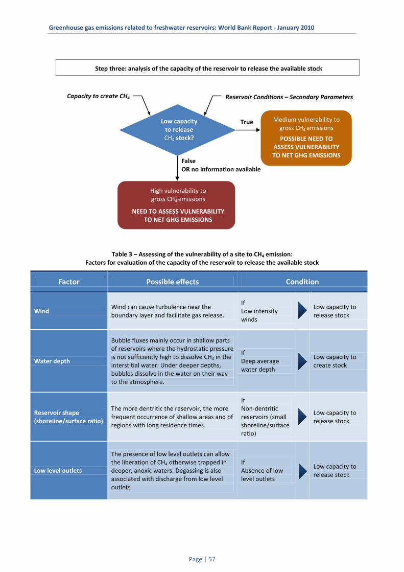
Greenhouse gas emissions related to freshwater reservoirs: World Bank Report - January 2010
Page | 57
Table 3 – Assessing of the vulnerability of a site to CH4 emission: Factors for evaluation of the capacity of the reservoir to release the available stock
Factor Possible effects Condition
Wind Wind can cause turbulence near the boundary layer and facilitate gas release.
If Low intensity winds
Low capacity to release stock
Water depth
Bubble fluxes mainly occur in shallow parts of reservoirs where the hydrostatic pressure is not sufficiently high to dissolve CH4 in the interstitial water. Under deeper depths, bubbles dissolve in the water on their way to the atmosphere.
If Deep average water depth
Low capacity to create stock
Reservoir shape (shoreline/surface ratio)
The more dentritic the reservoir, the more frequent occurrence of shallow areas and of regions with long residence times.
If Non-dentritic reservoirs (small shoreline/surface ratio)
Low capacity to release stock
Low level outlets
The presence of low level outlets can allow the liberation of CH4 otherwise trapped in deeper, anoxic waters. Degassing is also associated with discharge from low level outlets
If Absence of low level outlets
Low capacity to release stock
Capacity to create CH4
Step three: analysis of the capacity of the reservoir to release the available stock
Reservoir Conditions – Secondary Parameters
Low capacity to release CH4 stock?
Medium vulnerability to gross CH4 emissions
POSSIBLE NEED TO ASSESS VULNERABILITY TO NET GHG EMISSIONS
True
False OR no information available
High vulnerability to gross CH4 emissions
NEED TO ASSESS VULNERABILITY TO NET GHG EMISSIONS

Greenhouse gas emissions related to freshwater reservoirs: World Bank Report - January 2010
Page | 58
5. Risk assessment of the vulnerability to N2O emission There is insufficient knowledge on N2O emissions from reservoirs to evaluate their importance; however, it should be noted that the global warming potential of N2O is 310 stronger than CO2 (UNFCCC, 2009) over a 100 year time horizon.
5.1. N2O - Main processes and pathways N2O is produced by both natural processes and human-related activities. Primary human-related sources of N2O are agricultural soil management, animal-manure management, sewage treatment, mobile and stationary combustion of fossil fuel, adipic acid production and nitric acid production. N2O is also produced naturally from a wide variety of biological sources in soil and water, particularly microbial action in wet tropical forests (US EPA, 2009b).
N2O is produced in soils by both nitrification and denitrification reactions. Nitrification is an aerobic microbial process that converts ammonium (NH4+) to nitrate (NO3-) in the presence of oxygen. During denitrification, nitrates are transformed into nitrogen (N2). Denitrification requires anoxic conditions, but denitrifying bacteria are facultative anaerobes (Schlesinger, 1997; Hahn et al., 2000).
The higher N2O emission from tropical conditions could reflect the influence of temperature on nitrification and denitrification reactions, as well as nitrogen availability, which is greater in tropical than in boreal and temperate forests (Sitaula and Bakken, 1993; Stange et al., 2000; Clein et al., 2002).
There are still significant uncertainties about the contribution of the individual sources to atmospheric N2O. Aquatic systems are considered to be significant, but not the dominant sources of
atmospheric N2O (IPCC, 1990). According to Mengis et al. (1997), N2O concentrations seem to be strongly correlated with O2 concentrations in lakes. In oxic waters below the mixed surface layer, N2O concentrations usually increase with decreasing O2 concentrations. N2O is produced in oxic epilimnia, in oxic hypolimnia and at oxic-anoxic boundaries, either in the water or at the sediment-water interface. It is consumed, however, in completely anoxic layers. Anoxic water layers were therefore N2O undersaturated. All studied lakes were sources for atmospheric N2O, including those with anoxic, N2O undersaturated hypolimnia. However, compared to agriculture, lakes seem not to contribute significantly to atmospheric N2O emissions (Mengis et al., 1997).
Very few studies have measured N2O fluxes in wetlands, for the simple reason that the water-saturated and anoxic soils typical of these systems offer particularly unfavourable conditions for N2O production. The nitrification rate is quite low in these systems because of very low oxygen content, pH and nitrogen availability (Bridgham et al., 2001). As for denitrification, it is often limited by the lack of nitrates, a direct consequence of slow nitrification rates (Regina et al., 1996).
5.2. Factors affecting N2O production in reservoirs: The following factors are taken into consideration in the decision tree analysis:
Site characteristics:
• rainfall; • water temperature; • soil type; • agricultural practices (no-till or reduced tillage).
Reservoir characteristics:
• operation drawdown zone exposure (changes in
water depth).

Greenhouse gas emissions related to freshwater reservoirs: World Bank Report - January 2010
Page | 59
5.3. Decision Tree Analysis – Assessing of the vulnerability of a site to N2O emission
Table 4 – Assessing of the vulnerability of a site to N2O emission: Factors for evaluation of Carbon and Nutrient availability and lability
Factor Possible effects Condition
Soil type in the catchment: nitrogen availability
N2O is produced in soils by both nitrification and denitrification reactions, depending on the presence of ammonium (NH4
+) or nitrates (NO3-).
If Low ammonium Low nitrates
Low nitrogen stock in the catchment
Land use in the catchment
Agricultural, urban, industrial and other human activities can increase nitrogen availability in the contributing area. Primary human-related sources of N2O are agricultural soil management, animal-manure management, sewage treatment, mobile and stationary combustion of fossil fuel, adipic acid production and nitric acid production
If Low anthropogenic activity (pristine conditions)*
Low nitrogen stock in the catchment
Temperature Temperature influences nitrification and denitrification reactions.
If Low temperatures
Less labile nitrogen in the catchment
Agricultural practices
Heavy utilisation of synthetic nitrogen fertilizers in crop production typically results in significantly more N2O emissions from agricultural soils.
If Less utilisation of synthetic nitrogen fertilizers
Low nitrogen stock in the catchment
Less intensive, low-tillage techniques lead to reduction of erosive processes, with consequent less labile nitrogen
If Less intensive practices
Less labile nitrogen in the catchment
Rainfall Intense rainfall can contribute to increase labile carbon and nutrients.
If Low intensity rainfall
Less labile nitrogen in the catchment
* Observe that the pristine characteristics can change after the reservoir is created
Step one: analysis of the capacity of the system to provide load to the reservoir
Catchment characteristics
Low nitrogen stock?
Non-labile Nitrogen 2
Low vulnerability to gross N2O emissions
END OF ANALYSIS
Low to medium vulnerability to gross N2O emissions
END OF ANALYSIS
True
True
False OR no information available
False OR no information available
GO TO STEP TWO

Greenhouse gas emissions related to freshwater reservoirs: World Bank Report - January 2010
Page | 60
Table 5 – Assessing of the vulnerability of a site to N2O emission: Factors for evaluation of the capacity of the reservoir to create stock
Factor Possible effects Condition
Drawdown zone exposure
The capacity to create N2O stock is mainly related to reservoir operational routines. There is reduced N2O production under anoxic conditions. The main factor to cause stock creation in the reservoir is associated with drawdown zone exposure, in response to changes in water depth, allowing conditions for nitrification processes. This process is more intense when the period of soil exposure is longer. Seasonal emptying of the reservoir will allow more opportunity for stock creation than weekly or daily variations
If Small extend of drawdown zone exposure
Low capacity to create stock
If Short periods (weekly variations) of drawdown zone exposure
Low capacity to create stock
Nitrogen Load
Step two: analysis of the capacity of the reservoir to create stock
Reservoir conditions – Primary Parameters
Low capacity to create
N2O stock?
Low to medium vulnerability to gross
N2O emissions
END OF ANALYSIS
True
False OR no information available
GO TO STEP THREE

Greenhouse gas emissions related to freshwater reservoirs: World Bank Report - January 2010
Page | 61
Table 6 – Assessing of the vulnerability of a site to N2O emission: Factors for evaluation of the capacity of the reservoir to release the available stock
Factor Possible effects Condition
Drawdown zone exposure
Similarly to the creation of the stock, its release is also associated with reservoir operation, due to drawdown zone exposure. This process is more intense when the period of soil exposure is longer.
If Small extend of drawdown zone exposure
Low capacity to release stock
If Short periods of drawdown zone exposure
Low capacity to release stock
Capacity to create N2O stock
Step three: analysis of the capacity of the reservoir to release the available stock
Low capacity to release N2O stock?
Reservoir Conditions – Secondary Parameters
Medium vulnerability to gross N2O emissions
POSSIBLE NEED TO ASSESS VULNERABILITY TO NET GHG EMISSIONS
True
False or No information available
High vulnerability to gross N2O emissions
NEED TO ASSESS VULNERABILITY TO NET GHG EMISSIONS
Capacity to create N2O stock

Greenhouse gas emissions related to freshwater reservoirs: World Bank Report - January 2010
Page | 62
References Bridgham S.D., Updegraff K., Pastor J. (2001) A
Comparison of Nutrient Availability Indices Along Ombrotrophic- Minerotrophic Gradient in Minnesota Wetlands. Soil Sci Soc Am J 65: 259-269.
Clein J.S., McGuire A.D., Zhang X. et al. (2002) Historical and Projected Carbon Balance of Mature Black Spruce Ecosystems across North America: The Role of Carbon-Nitrogen Interactions. Plant and Soil 242: 15-32.
Cole, J.J., Y.T. Praire, N.F. Caraco, W.H. McDowell, L.J. Tranvik, R.R. Striegl, C.M. Duarte, P. Kortelainen, J.A. Downing, J. Middleburg and J.M. Melack (2007) Plumbing the global carbon cycle: Integrating inland waters into the terrestrial carbon budget. Ecosystems: 10. 1007/s10021-006-9013-8.
Conrad, R. (1989) Control of methane production in terrestrial ecosystems. Pages 39-58. In M.O. Andrea and D.S. Schimel (eds.) Exchange of Trace Gases between Terrestrial Ecosystems and the Atmosphere. J.Wiley & Sons.
Fiedler S., Sommer M. (2000) Methane Emissions, Groundwater Levels, and Redox Potentials of Common Wetland Soils in a Temperature-Humid Climate. Glob Biogeochem Cycles 14(4): 1081-1093.
Guérin F., Abril G., Tremblay A. and Delmas R. (2008) Nitrous oxide emissions from tropical hydroelectric reservoirs. Geophysical Research Letters 35, doi:10.1029/2007GL033057.
Hahn M., Gartner K., Zechmeister-Boltenstern S. (2000) Greenhouse Gas Emissions (N2O, CO2, CH4) from Three Different Soils Near Vienna (Austria) with Different Water and Nitrogen Regimes. Die Bodenkultur 51(2): 115-125.
Happell J.D., Chanton J.P. (1993) Carbon Remineralization in a North Florida Swamp Forest: Effects of Water Level in the Pathways and Rates of Soil Organic Matter Decomposition. Glob Biogeochem Cycles 7(3):475-490.
IPCC (2001) Third Assessment Report, Climate Change 2001. Houghton J.T., Ding Y., Griggs D.J., Noguer M., Van der Linden P.J., Dai X., Maskell K., Johnson C.A., Published by IGES, Japan.
IPCC (1990) Climate Change. Cambridge, pp. XXI and 25-26.
Mengis M., Gächter R., Wehrli B. (1997) Sources and Sinks of Nitrous Oxide (N2O) in Deep Lakes. Biochemistry 38: 281-301.
Regina K., Nykänen H., Silvola J., Martikainen P.J., (1996) Fluxes of Nitrous Oxide from Boreal Peatlands as Affected by Peatland Type, Water Table Level and Nitrification Capacity. Biogeochemistry 35: 401-418.
Schlesinger W.H. (1997) Biogeochemistry: An Analysis of Global Change. 2nd ed Academic Press, San Diego, California.
Sitaula B.K., Bakken L.R. (1993) N2O Release from Spruce Forest Soil, Relation with Nitrification, CH4 Uptake, Temperature, Moisture and Fertilisation. Soil Biol Biochem 25: 1415-1421.
Stange F., Butterbach-Pahl K., Papen H., Zechmeister-Boltenstern S., Li C., Aber J. (2000) A Process-Oriented Model of N2O and NO Emissions from Forest Soils. 2nd Sensitivity Analysis and Validation. J Geophys Res 105(D4): 4385-4398.
TUCCI, C., et al., UNESCO/IHA; April 2008. Assessment of the GHG Status of Freshwater Reservoirs.
UNESCO/IHA (2009) Measurement Specification Guidance for Evaluating the GHG Status of Man-Made Freshwater Reservoirs. Edition 1, 4 June 2009.
UNFCCC (2009) Global Warming Potentials. Retrieved 28 September from: http://unfccc.int/ghg_data/items/3825.php
U.S. Environmental Protection Agency (EPA) (2009a) Climate Change. Climate Economics. International Analyses. Retrieved 28 September 2009 from: http://www.epa.gov/climatechange/economics/international.html
U.S. Environmental Protection Agency (EPA) (2009b) Nitrous Oxide. Sources and Emissions. Retrieved 28 September 2009 from: http://www.epa.gov/nitrousoxide/sources.html

Deliverable 3
Proposal for CDM Methodology Revision
January 2010

Greenhouse gas emissions related to freshwater reservoirs: World Bank Report - January 2010
Page | 64
Greenhouse gas emissions related to freshwater reservoirs: World Bank Report - January 2010
Page | 65
Summary
World Bank Contract 7150219
Deliverable 3: Proposal for CDM Methodology Revision
This document, comprising two parts - a Field Manual and a Calculation Manual - was developed for the World Bank by the International Hydropower Association (IHA) under the World Bank Contract 7150219, to fulfil the requirements for Deliverable 3 of the contract terms: Proposal containing clarifications or revisions to a new Clean Development Mechanism methodology.
The Clean Development Mechanism Executive Board (CDM EB) has ruled that reservoir-storage hydropower projects must meet specified power density (installed power generation capacity divided by the flooded surface area) thresholds in order to avoid risks associated with scientific uncertainty concerning GHG emissions from reservoirs. At present, the criterion is that hydroelectric power plants with power densities less than or equal to 4 W/m2 cannot receive CDM support. This criterion effectively excludes reservoir storage hydropower from the CDM. An exception to this is any project that can demonstrate GHG emissions from the reservoir would be negligible.
The Field Manual and the Calculation Manual were developed based on the concepts developed in the Guidelines presented as Deliverable 1 of the present World Bank Contract (Guidelines for net GHG measurements aiming at international standardisation and objective measurements that will ease comparison, transferability and global use of data). These manuals describe what, when, where and how to measure the relevant key parameters, and how to estimate the net GHG emissions (the GHG impact from the creation of freshwater reservoirs) from these measurements.
The Field Manual provides instructions on the field methods and equipment necessary to estimate GHG emissions, under pre- and post-impoundment conditions. It gives qualified technicians and scientists a protocol to make GHG emission measurements in the field. More specifically, the Field Manual includes instructions on how to conduct GHG measurements in terrestrial (forest, grass and peatland) and aquatic (wetland, lake, river and reservoir) ecosystems in terms of GHG emissions, and carbon and nitrogen stocks.
The Calculation Manual details the standard procedures that are needed to calculate net GHG emissions resulting from the creation of a reservoir in a river basin. This manual is designed to be used with the data obtained from the procedures described in the companion Field Manual.
The Field Manual and the Calculation Manual are proposed as the basis for a new CDM “tool” referenced in a revised “Approved Consolidated Methodology 002” (ACM002) or a “new methodology”. It is proposed that these manuals should provide the means to measure and calculate net GHG emissions of reservoir-storage hydropower projects currently excluded from the CDM.
This combined tool or methodology will allow a clear approach to calculating emissions from reservoirs and will include options for a standardised approach to measurement and calculation in the face of natural variability and data uncertainty. It will enable reservoir hydropower projects with low net GHG emissions to qualify for the CDM.
The Calculation Manual is in an early draft stage: this version constitutes a Framework and Annotated List of Contents, describing the proposed format, objectives, elements to be considered, and general structure. When complete this pair of documents will provide a new methodology for testing the suitability of reservoir-storage hydropower projects for support under the CDM. Further refinement will be progressed through the UNESCO/IHA GHG Research Project.

Greenhouse gas emissions related to freshwater reservoirs: World Bank Report - January 2010
Page | 66

Greenhouse gas emissions related to freshwater reservoirs: World Bank Report - January 2010
Page | 67
Deliverable 3a
Proposal for CDM Methodology Revision
Part A – Field Manual
January 2010

Greenhouse gas emissions related to freshwater reservoirs: World Bank Report - January 2010
Page | 68
Acknowledgements This deliverable was developed under the UNESCO/IHA Project – GHG Status of Freshwater Reservoirs Research Project (the UNESCO/IHA GHG Research Project), hosted by the International Hydropower Association (IHA), in collaboration with the International Hydrological Programme (IHP) of UNESCO and benefitted from the collaboration of numerous research institutions and scientists composing the UNESCO/IHA GHG Research Project Peer Review Group (the UNESCO/IHA Forum).
We would like to express our sincere appreciation of the work carried out by all experts who took part in the UNESCO/IHA Workshops, and acknowledge the very large number of constructive comments received.
Particularly, we would like to acknowledge the following experts, for their collaboration to this specific document: Julie Bastien, Pierre-David Beaudry, Marie-Claude Bonneville, Robin Bourgeois, Maud Demarty, Stéphane Descloux, Michael Fink, Michelle Garneau, Joel Goldenfum, Renée Gravel, Atle Harby, Stéphane Lorrain, Luc Pelletier, Michel Simoneau, Ian Strachan, Richard Taylor, Paul Toulouse, Alain Tremblay, Carlos Tucci.
Scientific proof reading: Dr.John Gash.

Greenhouse gas emissions related to freshwater reservoirs: World Bank Report - January 2010
Page | 69
Table of contents
1 Introduction ........................................................................................................................ 72
1.1 Context .............................................................................................................................................................. 72
1.2 Objectives ......................................................................................................................................................... 72
2 Sampling considerations ................................................................................ 72
2.1 Steps and principles in planning field surveys .................................................................................................. 72
2.2 Spatial resolution of sampling stations ........................................................................................................... 113
2.2.1 Horizontal resolution .......................................................................................................................... 80 2.2.1.1 Terrestrial ecosystems ...................................................................................................... 80
2.2.1.2 Aquatic ecosystems .......................................................................................................... 80 2.2.1.3 Drawdown zone ................................................................................................................ 81
2.2.2 Vertical resolution .............................................................................................................................. 81
2.2.2.1 Terrestrial ecosystems ...................................................................................................... 81 2.2.2.2 Aquatic ecosystems .......................................................................................................... 82
2.3 Temporal resolution of sampling ...................................................................................................................... 82
2.3.1 Terrestrial ecosystems ........................................................................................................................ 82 2.3.2 Aquatic ecosystems ............................................................................................................................ 82
2.4 Considerations for young and mature reservoirs ............................................................................................. 83
3 Terrestrial system methodologies .................................................. 83
3.1 GHG emissions .................................................................................................................................................. 83
3.1.1 Soil emissions – Soil incubation .......................................................................................................... 84 3.1.1.1 Soil collection .................................................................................................................... 84
3.1.1.2 Soil preparation ................................................................................................................ 84 3.1.1.3 Air incubation ................................................................................................................... 84
3.1.1.4 Water incubation .............................................................................................................. 85
3.1.2 Soil/low-vegetation emissions ............................................................................................................ 85
3.1.2.1 Chamber technique .......................................................................................................... 85 3.1.2.2 Eddy covariance tripods .................................................................................................... 89
3.1.3 Land cover emissions .......................................................................................................................... 89 3.1.3.1 Indirect net ecosystem production (NEP) measurements ................................................ 89
3.1.3.2 Direct net ecosystem exchange (NEE) measurements – Eddy covariance towers ............................................................................................................................... 91
3.2 Carbon stock ..................................................................................................................................................... 93
3.2.1 Aboveground carbon pools ................................................................................................................ 93 3.2.1.1 Biomass in trees ................................................................................................................ 93
3.2.1.2 Biomass in shrubs ............................................................................................................. 95 3.2.1.3 Biomass in grasslands and peatlands ............................................................................... 97
3.2.1.4 Dead organic matter in peatlands and grasslands ............................................................ 97
3.2.1.5 Dead organic matter in forests ......................................................................................... 97
3.2.2 Belowground carbon and nitrogen pools ........................................................................................... 98 3.2.2.1 Carbon and nitrogen in forest floors ................................................................................ 98

Greenhouse gas emissions related to freshwater reservoirs: World Bank Report - January 2010
Page | 70
3.2.2.2 Carbon and nitrogen in mineral soil ……………………………………………………………………………………………………98
3.2.2.3 Carbon in roots ............................................................................................................... 100 3.2.2.4 Dissolved organic carbon ................................................................................................ 100
3.2.3 Mass-to-carbon conversion .............................................................................................................. 100
3.2.4 Total terrestrial biomass ................................................................................................................... 101
4 Aquatic system methodologies ........................................................ 101
4.1 GHG emissions ................................................................................................................................................ 101
4.1.1 Diffusive surface flux ........................................................................................................................ 102 4.1.1.1 Floating chambers .......................................................................................................... 102
4.1.1.2 Eddy covariance towers .................................................................................................. 104 4.1.1.3 Thin boundary layer (TBL) ............................................................................................... 105
4.1.2 Bubbling – Measurements using funnels ......................................................................................... 110
4.1.2.1 Funnel design .................................................................................................................. 110 4.1.2.2 Collecting gas from funnels ............................................................................................ 111
4.1.2.3 Calculating bubbling fluxes ............................................................................................. 111
4.1.3 Downstream emissions .................................................................................................................... 113
4.1.3.1 Degassing ........................................................................................................................ 113 4.1.3.2 Fluxes in the downstream aquatic system ..................................................................... 114
4.2 Carbon stock ................................................................................................................................................... 114
4.2.1 Carbon availability in water column / transport............................................................................... 114 4.2.1.1 Dissolved organic matter (DOM) .................................................................................... 114 4.2.1.2 Total organic carbon (TOC) ............................................................................................. 115
4.2.1.3 Dissolved organic carbon (DOC) ..................................................................................... 115
4.2.1.4 Dissolved inorganic carbon (DIC) .................................................................................... 115 4.2.1.5 C:N:P ratio ....................................................................................................................... 115
4.2.1.6 Origin of organic matter – ∂13C analysis ......................................................................... 116
4.2.1.7 Collection of samples in the water column .................................................................... 116
4.2.1.8 Calculation of carbon transport ...................................................................................... 117 4.2.2 Carbon storage in sediments ............................................................................................................ 118
4.2.3 Determining total, organic and inorganic carbon (TC, TOC and TIC) ................................................ 119
5 Gas analysers and gas measurement technologies ................................................................................................................................... 120
5.1 Gas chromatography (GC) analysis ................................................................................................................. 120
5.2 Infrared gas analysers (IRGAs) ........................................................................................................................ 120
5.3 Automated systems ........................................................................................................................................ 120
6 Ancillary measurements .............................................................................. 121
6.1 Water quality .................................................................................................................................................. 121
6.1.1 Dissolved oxygen .............................................................................................................................. 122 6.1.2 Biological oxygen demand ................................................................................................................ 122
6.1.3 Chlorophyll a..................................................................................................................................... 122 6.1.4 Nitrogen and phosphorus ................................................................................................................. 122

Greenhouse gas emissions related to freshwater reservoirs: World Bank Report - January 2010
Page | 71
6.1.4.1 Ammonia nitrogen .......................................................................................................... 122 6.1.4.2 Total Kjeldahl nitrogen.................................................................................................... 123
6.1.4.3 Nitrites and nitrates ........................................................................................................ 123
6.1.4.4 Total phosphorus and orthophosphates ........................................................................ 123
6.1.5 Water colour ..................................................................................................................................... 123 6.1.6 Water transparency .......................................................................................................................... 123
6.1.7 Turbidity ........................................................................................................................................... 123 6.1.8 Suspended solids .............................................................................................................................. 124
6.1.9 Conductivity ...................................................................................................................................... 124 6.1.10 pH ..................................................................................................................................................... 124 6.1.11 Alkalinity ........................................................................................................................................... 124
6.2 Physical water variables .................................................................................................................................. 124
6.2.1 Water level ....................................................................................................................................... 124
6.2.2 Sediment discharge .......................................................................................................................... 124 6.2.3 Residence time ................................................................................................................................. 124 6.2.4 Wave height ...................................................................................................................................... 125
6.3 Climatic conditions .......................................................................................................................................... 125
6.3.1 Air temperature ................................................................................................................................ 125 6.3.2 Relative humidity .............................................................................................................................. 125
6.3.3 Wind direction .................................................................................................................................. 125 6.3.4 Precipitation ..................................................................................................................................... 125
6.3.5 Atmospheric GHG concentrations .................................................................................................... 125
7 Quality assurance and quality control ................................... 126
7.1 General considerations ................................................................................................................................... 126
7.2 Instruments ..................................................................................................................................................... 127
8 References ........................................................................................................................... 128
9 Appendices………………………………………………………………………………………………………………………135

Greenhouse gas emissions related to freshwater reservoirs: World Bank Report - January 2010
Page | 72
1 Introduction
1.1 Context Although not specifically targeted, reservoirs are considered to be potential GHG sources and are of major concern to the power industry. At present, there is worldwide debate concerning the role of freshwater reservoirs and their contribution to atmospheric GHG emissions. Most studies of reservoirs indicate that GHG emissions can significantly vary (up to two orders of magnitude), from one reservoir to another, or even in the same reservoir for samples collected at different times of the year. Studies have been conducted primarily in Canada, Finland, Brazil, French Guiana and Laos.
Until now, there has been no worldwide standard procedure proposed for measuring GHG emissions from reservoirs and there is a lack of information on relevant ecosystems around the world. The UNESCO/IHA project has drafted a scoping paper (Tucci, C., 2008) covering the state of the art in 2008, and a document providing measurement specification guidance for GHG measurements (UNESCO/IHA, 2009). Complementing that document, this Field Manual presents succinct instructions for field methods and equipment needed to estimate net GHG emissions from all types of man-made reservoirs.
The approach (Section 2) to estimating the net GHG emission rate from reservoirs requires a comparison of pre-impoundment and post-impoundment fluxes from aquatic and terrestrial components. Variables to be measured and instruments for estimating terrestrial (Section 3) and aquatic (Section 4) emissions are presented. Also, gas analysers are briefly reviewed (Section 5), ancillary variables are listed and standard protocols are given as example (Section 6). Finally, general quality assurance and quality control (QA/QC) items are presented (Section 7). Specific QA/QC items are included within the specific method when required.
1.2 Objectives The main objective of this Field Manual is to provide objective and clear instructions on field methods and the equipment necessary to estimate GHG emissions, through field measurements of pre- and post-impoundment conditions, allowing qualified technicians and scientists to be able to
make field GHG emission measurements in freshwater reservoirs. More specifically, the Field Manual includes instructions on how to conduct GHG measurements in terrestrial (forest and peatland) and aquatic (wetland, lake, river and reservoir) ecosystems in terms of GHG emissions and carbon and nitrogen stocks.
This Field Manual may be updated to include new methodologies or instruments.
2 Sampling Considerations
Figures 2.1 and 2.2 present factors to be considered when developing a sampling plan, including station selection, spatial and temporal resolution, and monitoring. Details are given in the sections below. Figures 2.3 and 2.4 provide a summary of aquatic and terrestrial variables, associated methodologies, and advantages and constraints of those methodologies.
2.1 Steps and principles in planning field suveys
The following items should be considered when planning field surveys (ASTM, 1997; UNFCCC, 2009; Appendix 1 – Draft General Guidelines on Sampling and Surveys):
A. Scoping the project
• Describe the scope, approach to sampling and justification for it at an early stage.
• Specify objectives, site boundaries (Figure 2.5) and other scoping variables.
• Field campaigns should be planned by skilled personnel knowing the field and understanding the regional features affecting the project.
B. Literature/data review
• Collect existing pertinent data and information about the study site. Consult the literature and historical
records, and interview experts and government officials.
Consult topographic, geological, soil, vegetation and land use maps, aerial photographs and satellite images.

Greenhouse gas emissions related to freshwater reservoirs: World Bank Report - January 2010
Page | 73
Determine site history (changes in land use).
For terrestrial ecosystems, important variables include vegetation type, age of stand, soil type and regional climate.
For aquatic ecosystems, important variables include sediment type, present water level, changes in water level, water flows, depth, and reservoir operating procedures.
• Perform site reconnaissance to check the accuracy of available information and to identify site characteristics requiring further investigation.
C. Developing a sampling plan
• The purpose of sampling is to obtain reliable, unbiased estimates of the mean or total value of key variables. Reliability can be expressed in terms of the probability that the sample value falls within a specified interval around the population value.
• The accuracy of a sample-based estimate increases directly with sample size. Prior to taking a sample, the size required to achieve a given accuracy must be determined.
• The choice of sample type depends on several factors, including the types of information to be collected through sampling, known characteristics of the population, and the cost of information gathering. The sampling approaches include simple
random, systematic, stratified random, cluster and multi-stage sampling.
As the area covered by the reservoir and its watershed can be very large and influenced by land use, climate, geology, soil and reservoir characteristics, stratified sampling should be preferred over other sampling approaches whenever possible, i.e., whenever grouping variables are available. This approach consists of grouping cases into fairly homogeneous subpopulations and sampling each population independently. Stratification can increase efficiency through a gain in precision for a given sample size, and can ensure that estimates are made with equal accuracy within the various strata.
• Develop one or more conceptual models of the site based on existing information. Prepare maps of the study site.
• Develop a detailed site investigation and sampling plan. Review avai lable regional and
local in formation .
Interpret aerial photographs and other remote sensing data.
Select appropriate methods for collecting location data (latitude, longitude and altitude).
• Every project is site-specific and thus should have its own spatial and temporal planning for measurements.
• Spatial and temporal resolutions are linked, and a balanced approach is required in considering both. For example, if greater spatial than temporal variation is expected in a specific instance, more stations may be visited less frequently. If the opposite is true, a few representative stations may be visited more often or measurements may be taken continuously. The budget and resources available may influence planning.
• It is necessary to compartmentalise measurements in space and time to obtain representative measurements and to take into account any zones with high emissions but having a small surface area (or small number of occurrences over time).
• As a general principle, flow-proportional sampling should be applied, i.e., more measurements should be performed in compartments (or at times) of higher expected flux. For example, an area (or period of day) with 50% of the expected flux should be covered by 50% of the measurements.
• The same principles should be applied for pre- and post-impoundment measurements, for different systems (aquatic, terrestrial, downstream, upstream, etc.) and for different variables (GHG concentrations and fluxes, physical, chemical and biological variables, etc.).
• The spatial and temporal resolution must be subject to cost-benefit analysis and may be modified for budgetary reasons.
• Reference sites must be identified in both the aquatic and terrestrial ecosystems to ensure that normal variations due to climate or changes in land use are taken into account and not seen as reservoir effects. Reference sites may also be used to estimate net emissions when measurements begin after reservoir impoundment.
• Replicate measurements must be used in the field to account for the variation within the method (for example, three diffusive fluxes may be measured with the chamber method). Replicate analysis can also be performed to account for the variation within the analysis

Greenhouse gas emissions related to freshwater reservoirs: World Bank Report - January 2010
Page | 74
method (for example, three subsamples may be analysed by gas chromatography).
D. Field surveys
• Perform field reconnaissance and on-site investigation.
• Obtain representative samples and measurements for variables identified and selected.
• Collect field samples and take measurements.
E. Data analysis and sampling plan optimisation
• Analyse field and laboratory data. • Assess spatial resolution of selected variables.
Horizontal (surface): Upstream of the river/reservoir (in both the river and catchment), in the river/reservoir (in the river channel and drawdown zone), and downstream of the river/reservoir (in both aquatic and terrestrial systems)
Vertical (depth)
• Assess temporal resolution of selected variables potentially affecting GHG emissions. Diurnal – Light intensity, primary
production and respiration rate Seasonal – Wet and dry season, ice cover,
snowmelt and seasonal mixing of water Annual – Climatic conditions (precipitation,
runoff, temperature, etc.) and reservoir operating mode (water level)
• Refine the sampling plan based on the analysis of results. This is an iterative process whose length depends on the complexity of the study site and budgetary constraints. The results and analysis from an initial comprehensive survey will help determine hot spots, so continuous or seasonal measurements may be taken at a smaller number of representative sampling stations.
• Resolution must be an integral part of both planning and evaluation, using an adaptive measurement design (i.e., revising the resolution after analysing the initial data).

Greenhouse gas emissions related to freshwater reservoirs: World Bank Report - January 2010
Page | 75
Figure 2.1 — Scope of GHG monitoring program for reservoirs

Greenhouse gas emissions related to freshwater reservoirs: World Bank Report - January 2010
Page | 76
Figure 2.2 — Spatial and temporal resolution of sampling plan

Greenhouse gas emissions related to freshwater reservoirs: World Bank Report - January 2010
Page | 77
Figure 2.3 —Aquatic and terrestrial systems methodologies

Greenhouse gas emissions related to freshwater reservoirs: World Bank Report - January 2010
Page | 78
Figure 2.4.1 — Aquatic systems methodologies – pros and cons

Greenhouse gas emissions related to freshwater reservoirs: World Bank Report - January 2010
Page | 79
Figure 2.4.2 — Terrestrial systems methodologies – pros and cons
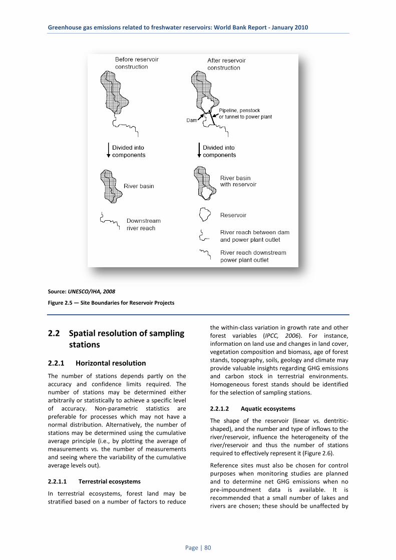
Greenhouse gas emissions related to freshwater reservoirs: World Bank Report - January 2010
Page | 80
Source: UNESCO/IHA, 2008
Figure 2.5 — Site Boundaries for Reservoir Projects
2.2 Spatial resolution of sampling stations
2.2.1 Horizontal resolution
The number of stations depends partly on the accuracy and confidence limits required. The number of stations may be determined either arbitrarily or statistically to achieve a specific level of accuracy. Non-parametric statistics are preferable for processes which may not have a normal distribution. Alternatively, the number of stations may be determined using the cumulative average principle (i.e., by plotting the average of measurements vs. the number of measurements and seeing where the variability of the cumulative average levels out).
2.2.1.1 Terrestrial ecosystems
In terrestrial ecosystems, forest land may be stratified based on a number of factors to reduce
the within-class variation in growth rate and other forest variables (IPCC, 2006). For instance, information on land use and changes in land cover, vegetation composition and biomass, age of forest stands, topography, soils, geology and climate may provide valuable insights regarding GHG emissions and carbon stock in terrestrial environments. Homogeneous forest stands should be identified for the selection of sampling stations.
2.2.1.2 Aquatic ecosystems
The shape of the reservoir (linear vs. dentritic-shaped), and the number and type of inflows to the river/reservoir, influence the heterogeneity of the river/reservoir and thus the number of stations required to effectively represent it (Figure 2.6).
Reference sites must also be chosen for control purposes when monitoring studies are planned and to determine net GHG emissions when no pre-impoundment data is available. It is recommended that a small number of lakes and rivers are chosen; these should be unaffected by

Greenhouse gas emissions related to freshwater reservoirs: World Bank Report - January 2010
Page | 81
anthropogenic water level fluctuations and located near the reservoir.
It is mandatory to have at least one representative station upstream, one within and one downstream of the river/reservoir so inflows and outflows to the river/reservoir can be monitored before and after impoundment.
Diffusion is expected to occur over the entire surface of the reservoir; whereas, bubbling is more likely to occur in the area where the depth is between 1 to 10m. The horizontal resolution at a sampling station will thus vary, depending upon the GHG emission pathway being measured or estimated.
2.2.1.3 Drawdown zone
All aquatic stations should be classified as being either in the drawdown zone or in the permanently flooded water body, because GHG emissions differ between these zones due to the presence/absence of vegetation. A representative station should be identified in each category. The period when the drawdown zone is flooded should be identified so that stations there can be identified as terrestrial or aquatic, and so that all seasons (with their varying water levels) are sampled equally. Diffusion and bubbling emissions can be expected to occur in the drawdown zone.
Figure 2.6 — Reservoir types
2.2.2 Vertical resolution
2.2.2.1 Terrestrial ecosystems
In terrestrial ecosystems, flux measurement systems determine the vertical resolution. Chambers and incubators measure emissions at
the soil-atmosphere interface while eddy covariance (EC) systems measure fluxes through the atmosphere above the land cover. Ideally, measurement from both strata (above the soil and above the land cover) should be taken, but this is usually not feasible.
Greenhouse gas emissions related to freshwater reservoirs: World Bank Report - January 2010
Page | 82
Carbon stock values may be estimated or measured at various levels: aboveground biomass from trees, shrubs and low vegetation, as well as belowground biomass from soil and roots. Carbon in soil should be measured at incremental depths up to 50 cm (e.g., 0–10 cm, 20–30 cm and 40–50 cm).
2.2.2.2 Aquatic ecosystems
In aquatic ecosystems, diffusive water-air interface GHG flux measurements/estimates are conducted at the water surface only using the floating chamber method or the thin boundary layer (TBL) method.
It is important to measure GHG concentrations at a number of depths near the water intake for degassing estimates (reservoirs only) and at other representative stations in the river/reservoir to determine the impact of water mixing in regions where this phenomenon occurs (boreal and temperate regions).
Water samples for carbon stock measurements should be collected at several depths to represent the entire water column.
Depth profiling of certain physico-chemical variables should be performed at a minimum number of stations to determine whether stratification occurs.
2.3 Temporal resolution of sampling Pre-impoundment inputs from the contributing areas should be determined prior to reservoir construction but may be measured after construction if the post-impoundment upstream catchment has not been changed from the pre-impoundment conditions or if reference sites nearby can be used. This will have an impact on net emission calculations (Figure 2.1: purple boxes). Temporal resolution must be established based on several criteria or sampling constraints as described below.
• Practicability. It is probably more practical to cover temporal variability by taking continuous measurements at a smaller number of measurement points, and to visit more points on a seasonal basis both to determine spatial variability and to validate the continuous measurements.
• Temporal variability at the study site. For example, young reservoirs are expected to vary more than mature reservoirs.
Continuous measurements should thus be favoured over field surveys in young reservoirs, at least during the initial years following impoundment.
• Spatial variability across the study site. Continuous measurements cannot be conducted at a large number of stations because of maintenance and cost constraints. Therefore, if the study site is homogeneous, continuous measurement can be conducted at a few selected representative stations.
When field surveys are the only option left, timing is important and must capture temporal (diurnal, seasonal and annual) variability. In each case, the extent of variation must be assessed, and then the sampling interval adjusted based on a cost-benefit analysis.
Annual variation is affected by study site age, climate (e.g., El Niño and climate change), land-use changes, extreme events (e.g., fires) and disease/pest outbreaks. Fires and disease/pest outbreaks will affect the terrestrial ecosystem directly, but also affect the aquatic ecosystem indirectly through leakage effects.
Seasonal variation is affected by seasons, hydrology/precipitation and drought. The number of field surveys per year will depend on seasonal variations specific to each region. In general, there should be from two (wet and dry seasons) to four (winter, spring, summer and autumn).
Nycthermal variation is affected by light intensity and temperature.
2.3.1 Terrestrial ecosystems
Emissions and carbon stocks (primary production and decomposition) from terrestrial ecosystems will vary with light intensity and temperature. Extreme event such as insect outbreak, fire, and drought can affect the terrestrial ecosystem dynamics, and subsequently the aquatic one via run-off. Both soil and land cover GHG flux measurements may be automated to provide continuous monitoring. If that is not possible, diurnal, seasonal and annual variations must be determined by a set number of field campaigns.
2.3.2 Aquatic ecosystems
Depending on the age of the reservoir, complexity of the site and available resources, a different frequency of measurements may be used at each site. The short-term dynamics of GHG emissions may be important and it may be necessary to consider semi-diurnal stratification processes in

Greenhouse gas emissions related to freshwater reservoirs: World Bank Report - January 2010
Page | 83
order to provide more accurate gas measurements. Ideally, variables should be measured automatically at fixed intervals (e.g., every three hours) during the day to account for diurnal variations. If that is not possible, nycthemeral variations (time of day and night) should be determined and a correction factor then applied to measurements.
Younger reservoirs require more frequent measurements than mature reservoirs during the initial years of monitoring. If there are major seasonal variations, at least four measurement campaigns per year are necessary, but monthly monitoring of key variables and GHG fluxes is likely to be required to capture seasonal variations and to provide robust mass balance measurements. Key variations in climatic and local conditions should be recorded in order to determine the sampling frequency and strategy.
The seasonal variation of the fluxes of the entire reservoir system (including the reservoir and river downstream) must be studied to accurately estimate reservoir emissions. Emissions may vary by more than one order of magnitude in the course of the year due to seasonal variations in organic carbon supply, age, thermal stratification, irregular convective mixing, depth and reservoir operations. Also, significant interannual variations have been observed. Statistical analysis should be applied to determine whether monitoring results in successive years are similar. If this is the case, future monitoring can be less frequent. If not, annual monitoring should continue until a steady state is reached. New reservoirs with high gross emissions may require longer periods of emission measurements than mature reservoirs.
2.4 Considerations for young and mature reservoirs
Young reservoirs are more prone to spatial variation due to their heterogeneous flooded area (vegetation and soil types). For example, flooded peatlands usually emit more than flooded lakes, rivers or forests in the first year following impoundment (Blais et al., 2007). This variation disappears as the reservoir ages (Bastien and Côté, 2007). Hence, more spatially distributed stations are necessary to account for spatial variability in young reservoirs. More frequent field surveys are also necessary to account for the initial increase and decrease in emissions following impoundment. Measurements in older reservoirs are not critical in that if, for any reason,
monitoring cannot be performed one year, it can the next with no major loss in information. This is not true for young reservoirs. Priority should always be given to monitoring young reservoirs first, and then older reservoirs.
The period of high initial GHG emissions characteristic of young reservoirs will vary in length (one to five years or more) depending on the quantity and type (lability and carbon content) of flooded vegetation and soil.
UNFCCC (2007; Appendix 1 – Proposed new baseline and monitoring methodologies for estimating GHG emissions from the Bumbuna Hydroelectric Project, Sierra Leone, CDM-NM00121) provides guidance on sampling approaches for reservoirs.
3 Terrestrial System Methodologies
The terrestrial component includes forests, peatlands, marshes and swamps. Marshes, swamps and peatland pools or ponds are at the limit between the terrestrial and aquatic ecosystems. The drawdown zone of reservoirs may be considered as a terrestrial or aquatic ecosystem depending on the water level. Marshes, swamps, peatland pools or ponds, and the drawdown zone of reservoirs may be studied and analysed using both terrestrial and aquatic variables and methodologies.
Measurement methods are discussed below under two separate headings: GHG emissions and carbon stock. GHG emissions in the terrestrial environment represent fluxes between the atmosphere and soils/low vegetation, and between the atmosphere and land cover. GHG emission methodologies use direct flux measurements. On the other hand, carbon stock variables are used to understand changes, and sometimes to estimate GHG emissions (indirect flux).
3.1 GHG emissions GHG emissions in terrestrial environments are dominated by CO2, CH4 and N2O. CO2 fluxes are expressed by the net ecosystem exchange (NEE) of CO2, which represents the balance between CO2 uptake through photosynthesis and release through respiration at a given moment in time.

Greenhouse gas emissions related to freshwater reservoirs: World Bank Report - January 2010
Page | 84
Net ecosystem productivity (NEP) represents the annual carbon stock change for a specific location, and includes CH4 fluxes, loss of carbon from forest fires and insect outbreaks, as well as dissolved organic carbon (DOC) export.
3.1.1 Soil emissions – Soil incubation
Soil emissions can be estimated by the soil incubation method. Two variants of the method can be used: air incubation, which provides an estimation of emissions in terrestrial environments, or water incubation, which provides an estimation of emissions in flooded environments.
The incubation method is used to estimate GHG emissions from specific soil types under predefined conditions. Soil samples are collected from the study area and taken to the laboratory where they are prepared according to the type of incubation to be performed, and then placed in incubators under controlled temperature and/or moisture conditions. Temperature-controlled rooms or incubators are necessary for this test. GHG emissions are measured by putting the incubated soil sample in a sealed container from which air samples are drawn over a given period of time. Samples are analysed on a gas chromatograph for CO2, CH4 and N2O concentration, and flux is calculated as the change in concentration over time.
3.1.1.1 Soil collection
A number of methods may be used to collect soil samples. The method selected depends on the type of soil (e.g., forest soil or peat) and on specific soil characteristics (e.g., grain size and root biomass). The number of samples and type of soils to be collected depends on the study area.
There are two methods for collecting soil samples in forest ecosystems: the square template and soil core methods. Generally, after removing the plant layer, the organic layer sample is collected using a knife and square template. The template, made of wood plastic or metal, is placed on the forest floor and the organic layer is sliced free using the knife inside the template. In mineral soil, a steel pipe or soil core (Figure 3.1) of known diameter (e.g., 5 cm) is driven into the soil to a known depth (e.g., 20 cm). In peat, samples are collected using a box corer (Figure 3.2), which allows simultaneous collection of both oxic and anoxic peat. The collected samples are placed in a sealed container, labelled and taken to the lab where they are kept in a refrigerator or a cold room at 4°C until preparation for incubation.
Source: Macaulay Soils
Figure 3.1 — Soil Cores
3.1.1.2 Soil preparation
Forest soil samples require preparation before incubation but this should be kept to a minimum to prevent unwanted mineralisation before incubation. For each layer collected, all soil sample replicates from the same sampling site are mixed together to obtain one sample per sample plot. Organic and mineral soil samples are sieved to remove roots, bark and stones, and to make the material homogeneous (Paré et al., 2006). Live sphagnum, wood debris and roots must be removed from peat samples.
Source: Macaulay Soils
Figure 3.2 — Box Corer
3.1.1.3 Air incubation
The air incubation method may be used to measure the release of GHGs through soil decomposition prior to reservoir impoundment. Temperature and moisture conditions during incubation should be representative of field conditions where samples were collected.

Greenhouse gas emissions related to freshwater reservoirs: World Bank Report - January 2010
Page | 85
A predetermined amount of soil (volume and weight) is placed in a container with a plastic mesh bottom. Paré et al. (2006) used 25 g of organic soil and 100 g of mineral soil in 150-ml containers. Soil samples are moistened until saturated and left to drain for 24 hours. The containers are then placed in an incubator or growth chamber under predefined temperature and moisture conditions.
GHG emissions may be measured 48 hours after the soil samples have been placed in the incubator. Measurements are made by taking the plastic container and its soil sample and placing it in a glass container with a metal lid (Masson jar) fitted with a septum. Once the glass jar is closed, gas samples are drawn from the headspace through the septum using a syringe fitted with a needle. Samples are analysed on a gas chromatograph. Flux is calculated as the change in concentration over time.
3.1.1.4 Water incubation
This type of incubation simulates soil flooded after reservoir impoundment and is used to measure potential GHG emissions. Temperature and oxygen level during incubation should be representative of reservoir conditions.
A predetermined amount of soil (volume and weight) is placed in a container. Thérien and Morrison (2005) used cylindrical quartz containers 300 mm in diameter and 300 mm in height for incubation. The container lid must be equipped with a septum for collecting gases and a tube connected to an O2 cylinder to oxygenate the water column and thus simulate oxic conditions. For anoxic tests, O2 must be flushed from the water and headspace of the container with nitrogen (N).
At the beginning of the test, the container is filled with a known volume of water from the river or lake to be dammed, leaving a headspace for gas to accumulate. It is important to monitor the water temperature, oxygen level and pH during the test. Flux can be calculated by measuring gas concentrations in the headspace and regressing them over the incubation time.
3.1.2 Soil/low-vegetation emissions
3.1.2.1 Chamber technique
The chamber technique is the most commonly used method of measuring gas exchange between soil/low vegetation and the atmosphere. Basically, the method consists in placing an open-bottom chamber on the soil surface and measuring the
change in GHG concentration over time (Weishampel and Kolka, 2008).
Different chamber designs (steady-state and non-steady-state) may be used to measure fluxes from soil and vegetation. This section will focus on non-steady-state (NSS) chamber design since most measurements from forest soils, agricultural systems and peatlands presented in the literature use this type of chamber. There are also many advantages in using this design: it is easy to build, the deployment time for flux measurements is shorter and low exchange rates may be measured.
Chamber shape and size, and material used will vary depending on the type of measurement to be made, height of vegetation and expected flux rates. The chamber design should be optimised for study site characteristics. If the chamber is too large, the rate of change in gas concentration will be small, and deployment time longer. If the chamber is too small, it may not be suitable for all heights of vegetation and the smaller area covered by the chamber may not adequately capture the spatial variability. Site accessibility and equipment transportation constraints must also be taken into account: larger chambers can be difficult to carry around.
Flux measurements of CO2, CH4 and N2O can be performed over a period ranging from 2 to 90 minutes or more. The flux measurement period must be established based on the chamber volume and the intensity of the respective fluxes. Low fluxes will require a longer measurement period in order to reach a good resolution. In the case of CO2 (NEE) measurements, flux rate should be looked at carefully before deciding on the length of measurement periods. When measuring photosynthesis by surface vegetation, CO2 concentration inside the chamber generally decreases over time. If the measurement period is too long, vegetation in the chamber is stressed because of the low CO2 concentration in the chamber. This can result in a variation in flux rate over time compared to the initial rate when beginning measurements. The flux measurement period should cover only the initial stage since vegetation is then under conditions closer to those in nature.
Ideally, measurement chambers should be fitted with a mixing fan to ensure adequate mixing of gases inside the chamber. Computer fans connected to a small battery outside the chamber are generally used. The size and number of fans should be a function of the volume and shape of the chamber. Tests should be performed before making final design decisions. The air displacement

Greenhouse gas emissions related to freshwater reservoirs: World Bank Report - January 2010
Page | 86
produced by the fan is also very important. It should approximate conditions in the environment where the measurements are to be made since wind speed may affect the rate of diffusion between the soil and chamber headspace. It is also an important factor when measuring net ecosystem exchange. Plant stomata tend to close when wind speed exceeds a certain level, and excessive wind speed can therefore alter CO2 absorption by the vegetation (de Langre, 2008).
Chamber flux measurements should be made using specially designed sampling collars or frames (Figure 3.3) permanently installed in the soil where the measurements are to be made. Installing such frames in the soil prior to measurements (from 1 hour beforehand in dry, bare sandy soil to several weeks in advance when roots need to grow back; Rochette and Bertrand, 2006) will minimize effects from disturbing the soil and damaging roots. The frames may be made of plastic or metal, and their shape will depend on the chamber design. Frames must have a groove in which the chamber can be fitted. When filled with water, this groove prevents air leakage between the chamber headspace and the atmosphere. It is also possible to use a rubber gasket and a fastener to clamp the chamber to the frame and ensure an airtight seal. It is important to avoid putting weight on the chamber even though that would help achieve an airtight seal. Pressure on the soil surface may induce the release of soil gases.
Source: Université du Québec à Montréal (UQAM)
Figure 3.3 — Plastic Collar Used for GHG Flux Measurements in Forests and Peatlands
Net ecosystem exchange (NEE) of CO2
NEE from low vegetation can be measured using clear NSS chambers (Figure 3.4). Measurement chambers are made of clear acrylic glass to allow light to enter, and therefore photosynthesis to occur. This type of chamber must be fitted with a cooling system to prevent the temperature inside from increasing (Table 3.1). Temperature increase inside the chamber could affect plant dynamics and related fluxes. Conditions inside the chamber should be kept as close as possible to ambient conditions at the time of measurement. Time of deployment should also be taken into consideration as it may be more difficult to control temperature over a long deployment time. NEE is measured by installing the chamber on the collar for a pre-defined period and by measuring CO2 concentration regularly over that period.
Source: Université du Québec à Montréal (UQAM)
Figure 3.4 — Clear Chamber for NEE Measurements
NEE measurements are made under different light intensities or levels of photosynthetically active radiation (PAR), which will affect flux magnitude and direction. Under clear blue skies, vegetation should be absorbing carbon dioxide, and therefore CO2 concentration in the chamber should be decreasing over the measurement period. At night, the system should be releasing CO2. Measurements are more difficult to make in the dark. To obtain CO2 measurements under different light levels, shrouds can be installed on the chamber to block part or all of the incoming light (Figure 3.5). These shrouds are made of mosquito netting. One or two layers of netting should block

Greenhouse gas emissions related to freshwater reservoirs: World Bank Report - January 2010
Page | 87
respectively 50% and 75% of the incoming PAR. A dark shrouds made with opaque fabric are used to measure dark respiration (PAR = 0). Measurements under different light levels (no shroud, 50% shroud, 25% shroud and dark shroud) should be made every time the site is visited for NEE measurements. The relationship between NEE and PAR can be obtained by regression of the NEE
flux value with the corresponding PAR measured inside the chamber at the time of measurement. The result obtained is an NEE-PAR or light response curve. The equation for this curve may later be used to model the fluxes over a longer period of time if continuous measurement of PAR is recorded.
Table 3.1 — List of Material for NEE (CO2) Measurements
Component Description
Chamber Transparent thermoplastic – acrylic glass
Frames or collars Plastic (e.g., machined blue plastic sewage pipes, see Figure 3.3) or metal
Fan Computer fan
In/out ports (air) Swedge lock fittings
Polyvinyl chloride tubing 1/8" (3 mm) ID (Fisher 14-169-7A)
In/out ports (water-cooling system) Brass Swagelok tube fitting, Bulkhead Union, 1/8" OD tube
Cooling system Coiled copper tubing, 1/16" (1.5 mm) ID, 1/8" (3 mm) OD (Cole-Parmer WU-34671-00)
Rule 500 Gph (2000 l/hr) bilge pump
Small cooler for water and ice
Infrared gas analyser for CO2 EGM-4 Environmental Gas Monitor for CO2
(PP Systems International, Inc., Massachusetts, USA)
PAR sensor PAR sensor (PP Systems International, Inc., Massachusetts, USA)
Source: Université du Québec à Montréal (UQAM)
Figure 3.5 — Chamber for NEE measurements covered with a shroud
CH4 and N2O fluxes
Chambers for CH4 and N2O flux measurements are generally made of acrylic plastic. Chambers must be opaque. Open-bottom 18-L water bottles have been used in various studies (Figure3.6). The chambers are covered with tin foil or thermal aluminium foil bubble insulation to prevent temperature increase inside (Table 3.2).
In order not to disturb the release of gases by inducing pressure on the soil near the chamber, it is recommended that wooden planks are installed in the area of the sampling sites. Samples may also be taken from the chambers through a 2-m tube with a 3-way stopcock attached to the chamber. If the chamber is not equipped with a fan, the air in the chamber headspace can be mixed prior to sampling using a 60-ml syringe. This would also ensure that the air in the 2-m tube is representative of that in the chamber headspace. The air samples may be collected in crimped pre-evacuated glass vials and analysed later on a gas chromatograph.
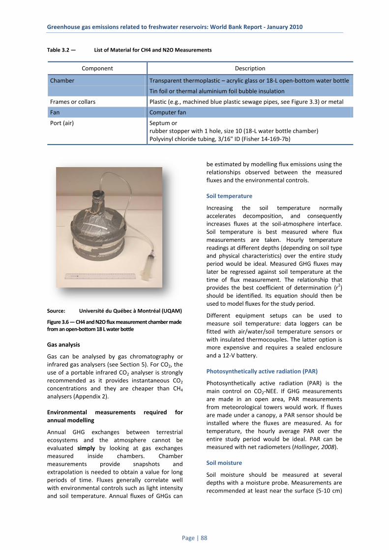
Greenhouse gas emissions related to freshwater reservoirs: World Bank Report - January 2010
Page | 88
Table 3.2 — List of Material for CH4 and N2O Measurements
Component Description
Chamber Transparent thermoplastic – acrylic glass or 18-L open-bottom water bottle
Tin foil or thermal aluminium foil bubble insulation
Frames or collars Plastic (e.g., machined blue plastic sewage pipes, see Figure 3.3) or metal
Fan Computer fan
Port (air) Septum or rubber stopper with 1 hole, size 10 (18-L water bottle chamber) Polyvinyl chloride tubing, 3/16" ID (Fisher 14-169-7b)
Source: Université du Québec à Montréal (UQAM)
Figure 3.6 — CH4 and N2O flux measurement chamber made from an open-bottom 18 L water bottle
Gas analysis
Gas can be analysed by gas chromatography or infrared gas analysers (see Section 5). For CO2, the use of a portable infrared CO2 analyser is strongly recommended as it provides instantaneous CO2 concentrations and they are cheaper than CH4 analysers (Appendix 2).
Environmental measurements required for annual modelling
Annual GHG exchanges between terrestrial ecosystems and the atmosphere cannot be evaluated simply by looking at gas exchanges measured inside chambers. Chamber measurements provide snapshots and extrapolation is needed to obtain a value for long periods of time. Fluxes generally correlate well with environmental controls such as light intensity and soil temperature. Annual fluxes of GHGs can
be estimated by modelling flux emissions using the relationships observed between the measured fluxes and the environmental controls.
Soil temperature
Increasing the soil temperature normally accelerates decomposition, and consequently increases fluxes at the soil-atmosphere interface. Soil temperature is best measured where flux measurements are taken. Hourly temperature readings at different depths (depending on soil type and physical characteristics) over the entire study period would be ideal. Measured GHG fluxes may later be regressed against soil temperature at the time of flux measurement. The relationship that provides the best coefficient of determination (r2) should be identified. Its equation should then be used to model fluxes for the study period.
Different equipment setups can be used to measure soil temperature: data loggers can be fitted with air/water/soil temperature sensors or with insulated thermocouples. The latter option is more expensive and requires a sealed enclosure and a 12-V battery.
Photosynthetically active radiation (PAR)
Photosynthetically active radiation (PAR) is the main control on CO2-NEE. If GHG measurements are made in an open area, PAR measurements from meteorological towers would work. If fluxes are made under a canopy, a PAR sensor should be installed where the fluxes are measured. As for temperature, the hourly average PAR over the entire study period would be ideal. PAR can be measured with net radiometers (Hollinger, 2008).
Soil moisture
Soil moisture should be measured at several depths with a moisture probe. Measurements are recommended at least near the surface (5-10 cm)

Greenhouse gas emissions related to freshwater reservoirs: World Bank Report - January 2010
Page | 89
and at mid-profile (50 cm) depths (Hollinger, 2008). A lot of moisture probes include integral temperature sensors (Hollinger, 2008).
3.1.2.2 Eddy covariance tripods
Eddy covariance measurements can be performed using tripods installed in low vegetation areas such as grasslands or peatlands. Eddy covariance is treated in Section 3.1.3.2 on direct measurements from land cover.
3.1.3 Land cover emissions
Indirect measurements of land cover emissions are based on net ecosystem production (NEP) estimates using measurements of the most important biological processes, while direct measurements of land cover emissions are based on net ecosystem exchange (NEE) estimates using eddy covariance or micrometeorology. NEP and NEE are equivalent terms that refer to the balance between uptake and release. However, NEP values usually have a positive sign to refer to accumulation of carbon by the system (the biologist’s standpoint) while NEE values usually have a negative sign to refer to absorption of carbon from the atmosphere (the meteorologist’s standpoint).
3.1.3.1 Indirect net ecosystem production (NEP) measurements
Indirect NEP estimation requires many types of measurements to cover all biological processes involved and is thus fraught with possible manipulation errors. Furthermore, it is practically impossible to measure all biological processes involved. Direct measurement of NEE should thus be preferred over indirect measurement, unless NEP (NPP and decomposition) values are available in the literature. Regardless of this, a good review of measurement methods for forest carbon monitoring is given in Field Measurements for Forest Carbon Monitoring (Hoover, 2008). The main processes to monitor and the names of frequently used methods are given below for information purposes without expanding on each.
Determining net primary production (NPP)
NPP estimates may be obtained from the literature or from a combination of measurements and allometric equations.
Available data from literature
NPP data from various vegetation types can be obtained from the literature (mainly governmental or national sources). For example, the Oak Ridge
National Laboratory’s Distributed Active Archive Center (ORNL DAAC) gives free access to NPP measurements from various sites around the world: http://daac.ornl.gov/NPP/npp_home.html
IPCC (2003) also presents aboveground NPP (ANPP) by climate zone. NPP values from the literature may be used to estimate NEP, but information must then be obtained for heterotrophic respiration or decomposition (see below).
Biometric measurements
NPP can be expressed as the sum of increments in live plant mass and dead plant mass, and increment lost to herbivory:
HDLNPP ++=
where L is the increment in live plant mass, D is the increment in dead plant mass, and H is the increment lost to herbivory (Curtis et al., 2002).
Increment in live plant mass L: Annual wood increment can be estimated by measuring the change in diameter at breast height (DBH) using band dendrometers (Curtis et al., 2002). The average annual increment in aboveground biomass by broad category and for all continents is also available from IPCC (2003).
Increment in dead plant mass D: Annual production of fine litter (leaves, flowers, fruits, etc.), or litterfall, can be estimated by using baskets placed on the forest floor. Baskets are emptied periodically, and their contents are dried and weighed (Curtis et al., 2002; Bernier et al., 2008). Branchfall can be estimated by a combination of fine litterfall traps, forest floor branchfall traps and line transects for coarse woody debris (Bernier et al., 2008).
Increment lost to herbivory H: Loss of leaf carbon to herbivores is estimated by collecting leaves prior to abscission and comparing their remaining area to that of undamaged leaves of the same size (Curtis et al., 2002).
Determining heterotrophic respiration (Rh) or decomposition
Decomposition should be measured/estimated in three compartments: dead wood, litter and soil. Soil decomposition is the main contributor to Rh (Curtis et al., 2002).
Decomposition of down dead wood
Key factors affecting decomposition of dead wood are moisture, wood quality (density and chemistry), size (diameter and length), and

Greenhouse gas emissions related to freshwater reservoirs: World Bank Report - January 2010
Page | 90
position (contact with the ground) (Scott and Brown, 2008). The most common methods for measuring the decomposition of dead wood are based on chronosequences of dead-wood samples, the time series approach and measurements of rates of dead-wood respiration across a range of decay classes (Scott and Brown, 2008).
Litter decomposition
Litter decomposition rates are controlled by four main factors: temperature, moisture, litter quality and faunal community structure (Karberg et al., 2008). Methods of estimating litter decomposition employ mass balance, litter-bags, tethered leaves and the cohort layered screen approach (Karberg et al., 2008).
Soil decomposition
Soil decomposition (respiration by heterotrophs) is equal to total soil respiration minus root respiration (respiration by autotrophs). There are five main source of CO2 efflux from soil (total soil respiration): root respiration, rhizomicrobial respiration, decomposition of plant residues, the priming effect induced by root exudation or by addition of plant residues, and basal respiration by microbial decomposition of soil organic matter
(Kuzyakov, 2006). Kuzyakov (2006) summarises the methods for partitioning total CO2 efflux from soil into root-derived CO2 and soil organic matter (SOC)-derived CO2 (Figure 3.7). Other methods are then required to distinguish root-derived CO2 as being either root respiration or rhizomicrobial respiration (Kuzyakov, 2006). For both, isotopic and non-isotopic methods can be used (Kuzyakov, 2006). A review of approaches to estimating respiration by autotrophic and heterotrophic organisms in soil is also given by Kuzyakov and Larionova (2005).
Total soil respiration can be quantified using closed-system chambers, open-system chambers and flux gradient sensors (Bradford and Ryan, 2008). Closed-system chambers are commercially available for soil CO2 efflux measurements. However, there must be some means of separating root respiration from total soil respiration (see Kuzyakov, 2006, and Kuzyakov and Larionova, 2005), such as with models incorporating soil temperature and moisture (Tang et al., 2005) or by performing direct measurements of rhizosphere respiration (root and rhizomicrobial respiration) with potted plants in the laboratory or with a field root respiration chamber (Kutsch et al., 2001)
Source: Kuzyakov, 2006 Figure 3.7 — Source of CO2 Efflux from Soil

Greenhouse gas emissions related to freshwater reservoirs: World Bank Report - January 2010
Page | 91
Calculating net ecosystem production (NEP)
NEP is the difference between NPP and Rh:
)( SLWD RhRhRhNPPNEP ++−= −
Where RhD-W is heterotrophic respiration from dead wood, RhL is heterotrophic respiration from litter, and RhS is heterotrophic respiration from soil.
3.1.3.2 Direct net ecosystem exchange (NEE) measurements – Eddy covariance towers
Direct NEE measurements are made using micrometeorological techniques. These techniques can provide direct, continuous, large-spatial-scale measurements of NEE. The current standard in ecosystem-scale trace gas measurement is eddy covariance (EC). A global network of tower flux stations has arisen in the past few decades and continues to expand into more remote regions and less accessible ecosystems.
The eddy covariance method is the only flux measurement technique that allows direct measurement of the net ecosystem exchange (NEE) of CO2, i.e., the net vertical flux of CO2 over a given ecosystem (Baldocchi, 2003). Atmospheric scientists typically use the meteorological sign convention, where negative NEE values represent a net uptake of CO2 by the ecosystem, and positive values indicate a net release into the atmosphere. NEE relies on the movement of the atmosphere where individual turbulent eddies transport different scalars (CO2, H2O) away from and towards the surface. The net ecosystem exchange can be decomposed into the sum of a turbulent component, a storage component and an advective component.
In the atmosphere, turbulence occurs across a frequency spectrum. In order to measure the rapid fluctuations in concentrations and wind speeds, fast-response sensors are used and measurements are commonly recorded at 10 or 20 Hz (i.e., ten or twenty measurements per second). Measurements are then averaged, typically over a 30-minute period, which captures all turbulent fluctuations (operating at frequencies of less than 30 minutes), while excluding the influence of longer time scale phenomena (weather patterns). Using the high-frequency data, the turbulent vertical flux of CO2 (Fc), for instance, is obtained by the covariance between the instantaneous departure (w’) from the mean vertical wind speed with the instantaneous departure (C’) from the mean gas concentration as
CwFc ′′= ρ
where ρ is air density and the overbar indicates a time average.
The storage flux (Fs), i.e., the rate of change in storage of CO2 in the column of air below the instrumentation height, can be calculated based on Morgenstern et al. (2004) as
Fs = hm ρ a (Δ S c / Δt)
where hm is the measurement height, ρ a is the
mean molar density of dry air, and S c is the mean
CO2 mole mixing ratio. Δ S c is the difference between Sc of the subsequent and previous half-hours.
The use of eddy covariance relies on several assumptions to ensure that what is measured adequately represents the surface of interest: the tower must be installed over a flat, uniform surface so that the average vertical wind speed is zero and flow divergence or convergence is negligible (thus making it possible to ignore the advective component, which is difficult to measure); the flow is fully turbulent so that transport is by turbulent eddies; the upwind edge of the surface of interest is sufficiently far away for the boundary layer to have fully adjusted to the surface of interest; and the position of the tower represents the ecosystem of interest for most of the prevailing wind directions.
Use and applications
The main instruments used in EC are the three-dimensional sonic anemometer, which measures wind speed along three axes (the mean flow direction, perpendicular to the mean flow, and vertically), and an infrared gas analyser (both open-path and closed-path IRGAs can be used), which measures the concentration of CO2 and water vapour. A fast-response thermocouple is often added for the measurement of sensible heat flux. Instrumentation has now also become available for fast-response measurement of methane concentration. A fast-response data logger is used to operate the system control and data handling programs. Fluxes are typically calculated in real time and are saved along with the raw high-frequency data on 1- or 2-GB compact flash cards. Depending on the application and sampling frequency, autonomous readings for up to one month are possible.

Greenhouse gas emissions related to freshwater reservoirs: World Bank Report - January 2010
Page | 92
EC instruments are mounted on the top of tripods (e.g., in peatlands) or on tall towers (e.g., in forests), and oriented toward the dominant wind direction. These systems are supplemented by standard meteorological instrumentation, including short- and long-wave radiative inputs and outputs, temperature, humidity, precipitation, and wind speed and direction. Several good reviews of eddy covariance methods, instrumentation and assumptions have been published (e.g., Goulden et al., 1996; Lee et al., 2004; Moncreiff et al., 1996; Pattey et al., 2006).
The main advantage of the EC method is that it provides continuous, spatially averaged measurement of the net vertical exchange of carbon, energy and water between the atmosphere and a surface, with minimal disturbance to the environment. The source area or flux footprint (i.e., the area upwind of the tower that is contributing to the measured fluxes), can be hundreds of square metres in size depending on instrumentation height, surface roughness and thermal stability. Schmid (1994; 2002) gives good definitions and approaches for calculating source areas. Data sets enable interpretation and comparison of GHG emission patterns on multiple time scales (hourly, seasonally or annually). EC can also provide winter emissions, which are often lacking with other techniques.
Such systems have been used successfully in remote field settings. Typically, power is supplied through deep-cycle marine 12-V batteries that are trickle-charged by a bank of solar cells or a wind generator system. When properly designed and insulated, such power systems run continuously year round, even through harsh northern winters. Where the power supply is an issue, the open-path IRGA is preferred because it does not require a pump and therefore power requirements are much lower. The open-path IRGA is limited in its use to periods without precipitation as the lens must be clear of physical obstruction. Where mains power is available, a closed-path IRGA can provide better all-weather data coverage. A cell modem can be used to communicate remotely with the logger. While transfer of the high-frequency data is not yet practical, this remote system check can be useful in timing the deployment of personnel to the field location.
Data processing for EC
With the EC technique, users must perform additional steps as part of the flux calculations, e.g., axis rotation, de-spiking, detrending and density corrections. Subsequent data processing includes thorough quality control and gap filling. Since the EC technique relies on turbulent
mixing of the air, one EC limitation is that it does not give good measurements during periods of low or intermittent turbulence, such as typically occur during calm nights. Data quality control must be performed to meticulously identify periods when data is not reliable. Such techniques often use a turbulence threshold criterion (e.g., friction velocity) for accepting data. Following quality control and after rejection of data due to instrument malfunction and maintenance, it is common that gaps occur in the data sets. Such gaps may, however, be filled using internationally accepted approaches based on models representing basic ecosystem processes (e.g., Falge et al., 2001). Since ecosystem respiration (ER) is mainly driven by temperature, an exponential relationship between night time NEE and soil temperature is commonly used to model ER for periods when gross ecosystem productivity (GEP) is assumed to be zero, i.e., at night and in the winter. This respiration model is also used to model day time respiration. Knowing that NEE = ER – GEP, it is possible to estimate GEP for the growing season. In terrestrial ecosystems, photosynthetic CO2 uptake is mostly controlled by photosynthetically active radiation (PAR). The “measured” GEP values are thus used to build a hyperbolic relationship between GEP and PAR, which allows the modelling of GEP when NEE is missing. The NEE time series can then be reconstructed by subtracting modelled GEP from ER for missing periods. This is why it is essential to continuously monitor meteorological variables. Such ancillary variables are also useful in examining the dominant factors controlling GHG fluxes in response to changes in environmental conditions.
In order to optimise the use of the EC technique, basic scientific knowledge of the physical properties of the atmosphere is required, along with some statistical background. The processing of EC data is quite complex and requires a significant amount of programming before the flux data can be used in a meaningful way. Most scientists using this technique use in-house scripts (e.g., Matlab) to perform the different processing steps. The use of this technique also requires regular calibration of the IRGA and maintenance of the systems. Significant person-hours are therefore required both in the field and for processing the data.

Greenhouse gas emissions related to freshwater reservoirs: World Bank Report - January 2010
Page | 93
3.2 Carbon stock The evaluation of the carbon stock present in the area to be flooded by the reservoir, and in reference terrestrial sites, is a critical measurement as it can be used as an indicator of future reservoir GHG emissions; GHG emissions are proportional to the content of organic matter flooded.
Biomass includes aboveground and belowground biomass. This living biomass consumes and produces CO2 by photosynthesis and respiration, respectively. Biomass gains include total biomass growth from the aboveground and belowground biomass. Losses are caused by decomposition, harvesting, burning or natural disturbances such as insects and diseases. Carbon stock also includes dead organic matter and carbon and nitrogen in forest floor and soils. Dead organic matter comprises dead wood and litter. Carbon from this carbon pool is emitted over years to decades as dead organic matter decomposes. Decay rates vary between climates and regions.
A good review of measurement methods for forest carbon monitoring is given in Field Measurements for Forest Carbon Monitoring (Hoover, 2008). The sections below outline the compartments where carbon stock should be measured and mention existing methods. Alternatively, values from the literature can be used to roughly estimate carbon stock from terrestrial environments if empirical data or pre-impoundment measurements are lacking, or to check the order of magnitude of measurements. For example, IPCC (2006) gives information on:
• Average aboveground forest biomass by domain, ecological zone and continent (Chapter 4)
• The ratio of belowground biomass to aboveground biomass for forests (Chapter 4)
• Average total grassland biomass (above- and belowground) by climate zone (Chapter 6)
Carbon stock from every compartment should be summed to determine the global carbon stock from the terrestrial ecosystem.
3.2.1 Aboveground carbon pools
Aboveground carbon pools include biomass in trees, shrubs, grasslands and peatlands, and dead organic matter in forests, peatlands and grasslands. The sections below present specific methods for estimating biomass from each type of vegetation and for estimating dead organic matter above ground.
3.2.1.1 Biomass in trees
Biomass in trees can be estimated based either on allometric equations using widely accepted forestry variables or on satellite imagery.
Allometric equations and biometric measurements
Aboveground biomass in live and standing dead trees can be estimated by allometric equations relating DBH to bole, branch and stump biomass (Curtis, 2008; Curtis et al., 2002). The total aboveground dry mass of an individual live tree i of species x can be estimated with a typical allometric equation of the form:
bxixi aDM =ˆ
where Dxi is diameter at breast height (1.37 m), and a and b are parameters obtained from species-specific fitted curves (Curtis, 2008). Plot-level aboveground mass, Mp, can be summed for n individuals of m species:
∑∑= =
=n
i
m
xxip MM
1 1
ˆ
There are two important points to consider when using allometric equations to estimate biomass (Curtis, 2008):
• Correction factors should be used if allometric parameters a and b were derived from logarithmic regressions. Those corrections factors are usually published along with allometric parameters a and b.
• Selection of the more species- and site-specific equations is critical. Species-specific and general hardwood equations are available in the literature for some parts of the world (Ter-Mikaelian and Korzukhin, 1997; Jenkins et al., 2003).
A snag is a standing dead tree with an angle of lean of 45° or less from the vertical (Curtis, 2008). Those leaning more than 45° are treated as dead organic matter (see Section 3.2.1.5). If the snag is not broken, it can be estimated from the living tree allometric equation as described above. Otherwise, the remaining bole wood volume must be estimated by measuring the snag height (H) with a clinometer, and the area at its base (Ab) and top (At) (Curtis, 2008). At can be measured from remains found on the ground or estimated visually. Two volume equations can be used, depending on whether the snag volume is estimated as a cone or paraboloid form (Curtis, 2008):
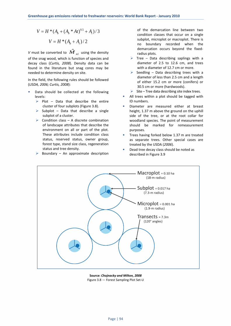
Greenhouse gas emissions related to freshwater reservoirs: World Bank Report - January 2010
Page | 94
3/))*((* 5.0tbb AAtAAHV ++=
2/)(* tb AAHV +=
V must be converted to xiM̂ using the density
of the snag wood, which is function of species and decay class (Curtis, 2008). Density data can be found in the literature but snag cores may be needed to determine density on site.
In the field, the following rules should be followed (USDA, 2006; Curtis, 2008):
• Data should be collected at the following levels: Plot – Data that describe the entire
cluster of four subplots (Figure 3.8). Subplot – Data that describe a single
subplot of a cluster. Condition class – A discrete combination
of landscape attributes that describe the environment on all or part of the plot. These attributes include condition class status, reserved status, owner group, forest type, stand size class, regeneration status and tree density.
Boundary – An approximate description
of the demarcation line between two condition classes that occur on a single subplot, microplot or macroplot. There is no boundary recorded when the demarcation occurs beyond the fixed-radius plots.
Tree – Data describing saplings with a diameter of 2.5 to 12.6 cm, and trees with a diameter of 12.7 cm or more.
Seedling – Data describing trees with a diameter of less than 2.5 cm and a length of either 15.2 cm or more (conifers) or 30.5 cm or more (hardwoods).
Site – Tree data describing site index trees. • All trees within a plot should be tagged with
ID numbers. • Diameter are measured either at breast
height, 1.37 m above the ground on the uphill side of the tree, or at the root collar for woodland species. The point of measurement should be marked for remeasurement purposes.
• Trees having forked below 1.37 m are treated as separate trees. Other special cases are treated by the USDA (2006).
• Dead tree decay class should be noted as described in Figure 3.9
Source: Chojnacky and Milton, 2008 Figure 3.8 — Forest Sampling Plot Set-U

Greenhouse gas emissions related to freshwater reservoirs: World Bank Report - January 2010
Page | 95
* Characteristics are for Douglas-fir. Dead trees of other species may vary somewhat. Use this only as a guide Source: USDA, 2006
Figure 3.9 — Tree Decay Class
Handbooks on forest ecosystems and forest mensuration may be consulted for more details on allometric equations and biometric measurements. The USDA National Core Field Guide (Appendix 1 – Forest Inventory and Analysis National Core Field Guide. Volume 1, Field Data Collection Procedures for Phase 2 Plots) gives valuable information on field data collection.
Satellite imagery
Spatial and temporal variations in aboveground biomass can be derived from satellite remote sensing data. First, a field-based relationship between the normalised difference vegetation index (NDVI) and aboveground biomass must be established. Based on this relationship, available satellite imagery can then be used to extrapolate biomass to a larger area of similar vegetation. Spectral measurements in each quadrat are sampled with a field spectroradiometer. The NDVI is computed from red and NIR reflectance (Kobayashi and Kato, 2007).
3.2.1.2 Biomass in shrubs
A shrub is a woody plant that generally has multiple basal stems growing from the same root system. For this reason, specific biomass methods exist for shrubs, as described in Chojnacky and Milton (2008). Existing methods are described briefly below. In each method, shrub cover or
basal area is measured in the field, and biomass is estimated from those measurements (Chojnacky and Milton, 2008).
Transect intercept cover sampling
The point intercept method records shrub vegetation that intercept a pole perpendicular to a transect at specified sampling intervals (Chojnacky and Milton, 2008; Figure 3.10):
• Establish transects from the subplot centre (Figure 3.8).
• Offset shrub-measurement transects from deadwood transects to minimize site disturbance.
• At each sample point along the transect, record the highest intersection of vegetation hitting the pole. Alternatively, the highest intersection among height classes can be recorded for greater detail.
• Vegetation hits can be recorded at species or species group level, depending on the detail desired.
Decay class stage
(code)
Limbs and branches
Top % Bark
Remaining Sapwood presence
and condition* Heartwood condition*
1 All present Pointed 100 Intact; sound, incipient decay,
hard, original color Sound, hard, original color
2 Few limbs, no fine branches
May be broken
Variable Sloughing; advanced decay, fibrous,
firm to soft, light brown
Sound at base, incipient decay in outer edge of upper bole, hard,
light to reddish brown
3 Limb stubs only Broken Variable Sloughing; fibrous, soft, light
to reddish brown
Incipient decay at base, advanced decay throughout upper bole,
fibrous, hard to firm, reddish brown
4 Few or no stubs Broken Variable Sloughing; cubical, soft, reddish
to dark brown
Advanced decay at base, sloughing from upper bole, fibrous to cubical,
soft, dark reddish brown
5 None Broken Variable Gone
Sloughing, cubical, soft, dark brown, OR fibrous, very soft, dark
reddish, brown, encased in hardened shell

Greenhouse gas emissions related to freshwater reservoirs: World Bank Report - January 2010
Page | 96
Source: Chojnacky and Milton, 2008
Figure 3.10 — Shrub Point-Intercept Method
Percent shrub cover is calculated by summing the number of sample points where vegetation intersects, or hits, the pole and dividing by the total number of points sampled:
NP
er ijkN
ijk ∑
=
=1100cov
where jkercov
is the percent shrub cover for
height j of species or species group k and ijkP = 1 if
foliage intercepts sample pole at point i for height
layer j of species k and ijkP = 0 otherwise. N is the
total number of points sampled in layer j for all transects on the plot. An equation to convert shrub cover to biomass must then be constructed. Only a few equations exist in the literature.
The line-intercept method is a variant of the previous method that records vegetation cover by measuring the length (horizontal distance) of shrub cover that intersects the transect (Chojnacky and Milton, 2008; Figure 3.11).
Visual cover sampling
Visual cover can be estimated visually to the nearest percent or within predetermined cover classes (1%–5%, 6%–10%, 11%–20%, 21%–40%, 41%–60%, 61%–80% and 81%–100%). Visual cover estimates can be performed within identified (flagged) microplot boundaries using percentage area guides for aiding visual estimation. It is useful to divide the microplot into four quadrants, estimate each of them separately and then average the results (Chojnacky and Milton, 2008). Two or more persons can make independent estimates in order to reduce subjectivity. A variant of this method adapted for small shrubs consists in performing visual cover estimation in small quadrats (1 m2 or smaller) spaced along transects
radiating from each subplot (Chojnacky and Milton, 2008).
Source: Chojnacky and Milton, 2008
Figure 3.11 — Shrub Line-Intercept Method
Diameter measurements
In this method, the basal diameter of each shrub in a microplot is measured at the root collar (Chojnacky and Milton, 2008). A minimum diameter should be set to simplify measurements. Shrub stems not included because of their small diameter might be included in herbaceous cover measurements, or just ignored, given their small incremental value (little carbon content for the
field effort required). Total basal area ( kY ) for
species k (m2/ha) can be computed as follow:
∑=
=kS
i mp
ikk A
drcY1
2
000,40π
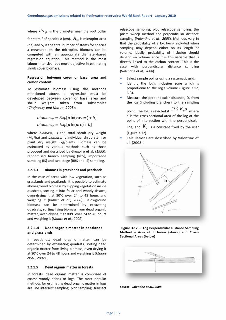
Greenhouse gas emissions related to freshwater reservoirs: World Bank Report - January 2010
Page | 97
where ikdrc is the diameter near the root collar
for stem i of species k (cm), mpA is microplot area
(ha) and Sk is the total number of stems for species k measured on the microplot. Biomass can be computed with an appropriate diameter-based regression equation. This method is the most labour-intensive, but more objective in estimating shrub cover biomass.
Regression between cover or basal area and carbon content
To estimate biomass using the methods mentioned above, a regression must be developed between cover or basal area and shrub weights taken from subsamples (Chojnacky and Milton, 2008):
])ln([])ln(cov[
bdrcaExpbiomassberaExpbiomass
P
T
+=+=
where biomassT is the total shrub dry weight (Mg/ha) and biomassP is individual shrub stem or plant dry weight (kg/plant). Biomass can be estimated by various methods such as those proposed and described by Gregoire et al. (1995): randomised branch sampling (RBS), importance sampling (IS) and two-stage (RBS and IS) sampling.
3.2.1.3 Biomass in grasslands and peatlands
In the case of areas with low vegetation, such as grasslands and peatlands, it is possible to estimate aboveground biomass by clipping vegetation inside quadrats, sorting it into foliar and woody tissues, oven-drying it at 80°C over 24 to 48 hours and weighing it (Bubier et al., 2006). Belowground biomass can be determined by excavating quadrats, sorting living biomass from dead organic matter, oven-drying it at 80°C over 24 to 48 hours and weighing it (Moore et al., 2002).
3.2.1.4 Dead organic matter in peatlands and grasslands
In peatlands, dead organic matter can be determined by excavating quadrats, sorting dead organic matter from living biomass, oven-drying it at 80°C over 24 to 48 hours and weighing it (Moore et al., 2002).
3.2.1.5 Dead organic matter in forests
In forests, dead organic matter is comprised of coarse woody debris or logs. The most popular methods for estimating dead organic matter in logs are line intersect sampling, plot sampling, transect
relascope sampling, plot relascope sampling, the prism sweep method and perpendicular distance sampling (Valentine et al., 2008). Methods vary in that the probability of a log being included when sampling may depend either on its length or volume. Ideally, probability of inclusion should depend on volume since it is this variable that is directly linked to the carbon content. This is the case with perpendicular distance sampling (Valentine et al., 2008):
• Select sample points using a systematic grid. • Identify the log’s inclusion zone which is
proportional to the log’s volume (Figure 3.12, left).
• Measure the perpendicular distance, D, from the log (including branches) to the sampling
point. The log is selected if aKD v≤ where a is the cross-sectional area of the log at the point of intersection with the perpendicular
line, and vK is a constant fixed by the user
(Figure 3.12). • Calculations are described by Valentine et
al. (2008).
Figure 3.12 — Log Perpendicular Distance Sampling Method – Area of Inclusion (above) and Cross-Sectional Areas (below)
Source: Valentine et al., 2008

Greenhouse gas emissions related to freshwater reservoirs: World Bank Report - January 2010
Page | 98
3.2.2 Below-ground carbon and nitrogen pools
Below-ground carbon and nitrogen pools include the forest floor (organic horizons), the mineral soil carbon content (mineral horizons), and root biomass (Burton and Pregitzer, 2008). Soil carbon stocks are one of the largest carbon pools in forest and wildland ecosystems (Burton and Pregitzer, 2008). Coarse root biomass can also be a large pool with typical values of around 20% to 30% of the aboveground carbon content in wood (Burton and Pregitzer, 2008).
Soil classification may be required to identify the type of horizons likely to be found in the project area. Classification typically distinguishes the organic (L, F, H) and mineral (A, B, C) horizons. Soils are a mixture of organic and inorganic constituents that are in solid, gaseous and aqueous states. The soil lies below the litter and has a smaller particle size. Organic soils (peat and muck) have a minimum of 12% to 20% of organic matter by mass, whereas all other soils are considered mineral soils (IPCC, 2006).
3.2.2.1 Carbon and nitrogen in forest floors
Forest floors can be sampled using 30- x 30-cm frames, separating material from each organic horizons, drying at 70°C for 48 hours, weighing, grinding, and analysing for elemental carbon (Burton and Pregitzer, 2008).
3.2.2.2 Carbon and nitrogen in mineral soil
Mineral soil carbon content can be obtained using volumetric pits or core sampling to a depth of at least 30 cm for annual vegetation, and 60 cm or more for perennial vegetation (Ellert et al., 2008; Burton and Pregitzer, 2008). Beneath 70 cm, additional samples for soil carbon and nitrogen analysis may be obtained using soil augers (Burton and Pregitzer, 2008). As a general rule samples should be collect to a depth of 50 cm and taken at incremental depths (for example: 0-10 cm, 20-30 cm and 40-50 cm).
A. QA/QC procedures should include the following steps (Burton and Pregitzer, 2008; MDDEP, 2008):
• Wash and brush sampling instruments, e.g., shovel, corer, auger or tube (Figure 3.13), with water, acetone, hexane and again with acetone, in that order, to prevent contamination of soil samples. Washing should be performed between each sampling site and each depth increment.
Washing liquids should be recovered and disposed of in an appropriate place. Instruments may be wrapped in aluminium foil between washing and sampling.
• Perform mineral soil carbon content sampling first and then forest floor sampling at the same sites to avoid mixing litter or organic horizons with the mineral horizons.
• Perform pit widening between depth increments (Figure 3.14).
• Mix samples from each depth separately to obtain a homogeneous mixture. If the soil contains large particles (> 2 mm), it should be sieved to collect only the fine portion, which is more subject to bacterial degradation.
• Fill glass bottles (250 ml) with soil using a spoon or spatula. Do not leave any free space. The laboratory usually supplies pre-washed glass bottles.
• Take 10% of the samples in duplicate. • Keep samples at 4°C in the dark before analysis. • Send samples to a specialised lab.
Alternatively, soil samples may be prepared and analysed using a TIC/TOC analyser as described in Section 4.2.3.
Figure 3.13 — Auger (above) and Tube (following page) for Soil Sampling

Greenhouse gas emissions related to freshwater reservoirs: World Bank Report - January 2010
Page | 99
Source: MDDEP, 2008
Source: Burton and Pregitzer 2008
Figure 3.14 — Pit Widening between Soil Depth Increment Sampling
B. Determine sample volume using the water method or foam method. The water method consists of placing a plastic bag in the core hole and recording the volume of water
required to fill the hole. The volume determination using the foam method involves the following steps:
Insert markers at each depth increment (pit widening should not have been performed).
Fill the entire core hole with polyurethane foam, place a cardboard and weight to seal the surface, and wait eight hours to let the foam expand and fill irregularities.
In the laboratory, foam casts are cut into segments corresponding to depth increments and sprayed with water-resistant clear-gloss urethane to create a waterproof seal.
The volume for each depth increment is determined by water displacement.
C. Separate the stone and soil fractions, and determine their density in order to ensure accurate estimates of carbon stock per unit area (Burton and Pregitzer, 2008; Figure 3.15).
D. The volume of stones is determined by their mass (MSt > 10 mm and 2–10 mm) divided by
their density (DSt): StStSt DMV /= .
The bulk density (DB) is determined by the total dry mass of all material (stones, organic material, soil < 2 mm, coarse roots and fine roots) in the depth increment divided by the total volume of the depth increment: TTB VMD /= .
The volume of the fine fraction (VF, < 2 mm) is equal to the total volume minus the volume of the stone fraction and the volume of the coarse-root fraction (VCR, > 10 mm in diameter):
CRStTF VVVV −−= .
The fine fraction density ( FD ) is
determined by the mass of the fine fraction ( FM ) divided by its volume:
FFF VMD /= .
Total carbon stock is obtained by adding the carbon stock (SC) of each depth increment sampled. Calculation of carbon stock for each depth increment is equal to:
T
OMOMFSFSIC V
MCMCTS )]()[( ×+××=
where IT is the thickness of the depth
increment, FSC is the carbon
concentration of material passing the

Greenhouse gas emissions related to freshwater reservoirs: World Bank Report - January 2010
Page | 100
2-mm screen, OMC is the carbon
concentration of organic material > 2 mm (other than coarse roots > 10 mm
in diameter), FSM is the mass of
material passing the 2-mm screen, OMM
is the mass of organic material > 2 mm and TV is the total volume of the depth
increment. The C:N ratio for each soil fraction should
be determined and used as an indicator of biological availability.
Figure 3.14 – Mineral Soil Sampling
3.2.2.3 Carbon in roots
Destructive methods exist for measuring carbon stored in root, but are labour-intensive. Belowground biomass can be derived from allometric equations relating DBH to woody root mass (Burton and Pregitzer, 2008). For most tree species, only general relationships are available, in which belowground wood mass is set at a fixed fraction of aboveground wood mass (Curtis et al., 2002). Alternatively, carbon concentration of all coarse roots may be assumed to be the same as coarse roots sampled within the soil pits (Burton and Pregitzer, 2008; see Section 3.2.2.2).
3.2.2.4 Dissolved organic carbon
Lysimeters are used to collect samples in unsaturated soils, while wells and piezometers are used where water tables are present (Kolka et al., 2008). Lysimeters can be installed between the
organic and mineral horizons to determine the flux of carbon between the two, and in or below the mineral horizon to determine the quantity of carbon leaving the ecosystem (Kolka et al., 2008). Filtration using a pore size of 0.45 μm is necessary to retrieve particulate organic carbon (Kolka et al., 2008). See Section 4.2.3 for elemental C analysis.
DOC fluxes can be estimated by multiplying DOC concentration by the water flux. At the watershed level, flow can be measured at a weir or flume (Kolka et al., 2008).
3.2.3 Mass-to-carbon conversion
The relation between biomass and carbon is species-specific and tissue-specific: the carbon content of woody mass varies across constituent tissues, such as bark, sapwood and hardwood, depending on tree species (Curtis, 2008). A bioassay should be performed to determine the

Greenhouse gas emissions related to freshwater reservoirs: World Bank Report - January 2010
Page | 101
actual relation between biomass and carbon. As a rule of thumb, the carbon content equals 50% of the biomass weight (Valentine et al., 2008). Some species-specific relations of biomass to carbon content are presented in Chapter 4 of IPCC (2006).
3.2.4 Total terrestrial biomass
Biomass measured or estimated from the aboveground (Section 3.2.1) and belowground (Section 3.2.2) pools should be summed to gauge the total terrestrial carbon stock. The DOC fraction (Section 3.2.2.4) of the total carbon stock is important to determine leakage of carbon between terrestrial and aquatic ecosystems.
4 Aquatic System Methodologies
Similarly to terrestrial ecosystems, aquatic ecosystems in the study site must be characterised before undertaking GHG measurements in order to understand spatial and temporal variations. For instance, information on bathymetry, flow conditions, sediment and changes in water level may provide valuable insights regarding GHG emissions and carbon stock in aquatic environments.
Measurement methods are discussed separately below for GHG emissions and carbon stock. GHG emissions in the aquatic environment represent fluxes between the atmosphere and water surface (diffusive flux) and bubbling from the sediment to the water surface. In reservoirs, a third emission pathway is possible at weirs, dams and spillways, where the rapid change in pressure favours degassing of less soluble gases. Carbon stock variables are used to understand changes in GHG emissions and may also be used as a proxy to estimate GHG emissions.
The International Organization for Standardization (ISO) provides guidance on sampling from lakes, natural and man-made, and on the design of sampling programmes and sampling techniques in aquatic systems (Appendix 1).
4.1 GHG emissions CO2, CH4 and N2O are three predominant GHGs emitted naturally by aquatic systems, the first two being the most important.
CO2 and CH4 gas concentrations in water can be influenced by several factors, including:
• mixing regime (for example, in boreal ecosystems, autumn and spring turnover transport the water enriched in dissolved gases from the bottom to the top of the water column);
• abundance of algae and plants, and their photosynthetic rates;
• quantity of organic matter entering the system and its decomposition rate in the water column and sediment (CH4 is produced in anoxic sediment by fermentation; Wang et al., 1996);
• water residence time, which affects dissolved organic matter availability;
• dissolved oxygen content, which affects the rate of CH4 consumption by methanotrophic bacteria (Wang et al., 1996).
N2O is an intermediate by-product of two microbiological processes — nitrification (aerobic process) and denitrification (anaerobic process) — which occur mainly at the sediment/water interface but could also take place in organic-matter-rich water columns. Although N2O has a global warming potential (GWP) 310 times greater than CO2 (UNFCCC, 2009), N2O fluxes are probably negligible in the overall GHG budget (which includes all three gases) as measured in boreal reservoirs and in one Brazilian reservoir (Table 4.1). Furthermore, Delmas et al. (2004) have shown that N2O fluxes varied little throughout the Petit Saut reservoir system (upstream of the impoundment, within the reservoir and downstream of the reservoir). This lack of variation indicates some kind of an equilibrium condition.
Higher N2O emissions may occur if there is a significant input of organic or inorganic nitrogen from the basin, e.g., input from such anthropogenic activities as land-use change, waste-water treatment or fertilizer application in the watershed (IPCC, 2006). It is important to note that in this case the emissions are not the result of reservoir creation but of external anthropogenic activities.
The sampling protocols for measuring N2O will be added to future versions of the Field Manual once more knowledge is achieved.

Greenhouse gas emissions related to freshwater reservoirs: World Bank Report - January 2010
Page | 102
Table 4.1 — N2O fluxes in boreal and tropical reservoirs and their importance in the overall budget
Reservoir Sampling
year
N2O (mg N2O/m2/d) % of total GHG emissions in
CO2eq Source
mean SD
Eastmain 1, Canada 2006 0.09 0.43 < 1% Tremblay and Bastien, 2009
Eastmain 1, Canada 2007 -0.02 0.44 < 1% Tremblay and Bastien, 2009
Experimental Lakes Area (ELA), Canada
2000 0.0012 0.0002 < 1% Hendzel et al., 2005
Experimental Lakes Area (ELA), Canada
2001 -0.0030 0.0006 < 1% Hendzel et al., 2005
Serra da Mesa, Brazil 2004 0.08 0.52 3% Sikar et al., 2005
4.1.1 Diffusive surface flux
4.1.1.1 Floating chambers
The floating chamber method is a cheap and convenient method to measure direct diffusive fluxes at the surface of aquatic ecosystems. This method consists of enclosing air in a chamber that floats at the surface of the water (Figure 4.1). Fluxes are then calculated according to the change of the concentration of the gas in the chamber (Abril et al. 2005, Guérin et al. 2007, Tremblay and Bastien 2009).
Diffusive fluxes depend on the concentration gradient between the surface microlayer and the atmosphere and physical variables such as wind speed and rainfall (Borges et al., 2004 a and b; Guérin et al., 2007). Artificial turbulence can be created by the chamber itself due to friction between the edges of the chamber and the water. When the chamber walls do not extend below the water surface, the chamber drifts creating turbulence which can generate gas fluxes up to five times higher in comparison to chambers with wall extensions into the water (Matthews et al., 2003). This becomes important at low wind speed (~1 m s−1) (Matthews et al., 2003). Thus, floating chambers must have walls extending below the waterline (Figure 4.1). In turbulent environments, the chamber can rock back and forth and bob up and down increasing the turbulence at the air-water interface. The chamber can be stabilised by weights attached to the bottom of the chamber skirt. It is important to stress that generally it is not necessary to weight the base of the chambers but then it cannot be used if strong waves are likely. The solubility of gases in water depends on pressure and temperature. When the pressure
increases, the solubility increases and vice versa. A vent must be installed on the top of the floating chamber in order to equilibrate the air pressure within the chamber with the atmospheric pressure before starting the measurements (Figures 4.1 and 4.2). In order to limit variation of temperature inside the chamber, the enclosure must be covered with reflective material. Typical dimensions and characteristics are as follows:
• height above the water surface while floating: 15 cm;
• chamber walls must extend 2-4 up to 15 cm below the water surface depending on the instability at the site caused by wind, waves, etc;
• minimum surface: 0.2 m² ; • volume: 20 L; • weight of the weights must be adapted: 500-
1000 g in order to adjust the penetration of the chamber walls.
As discussed by Kremer et al. (2003), a chamber that moves relative to the surface water would disrupt the aqueous boundary layer and artificially enhance gas exchange. If fluxes are not measured while floating freely with water movements this leads to a significant overestimation of the fluxes since turbulence is artificially enhanced by the friction between the chamber walls and the water. Thus, measurements must be performed while drifting with water at lake and river surfaces. However, in environments with low water current, but high wind, it is preferable to anchor the chamber to avoid its movement due to the wind, but in environments with high currents, drifting with water masses is necessary (Frankignoulle et al. 1996).

Greenhouse gas emissions related to freshwater reservoirs: World Bank Report - January 2010
Page | 103
Source: UNESCO/IHA, 2009 Figure 4.1 — Sketch of a Chamber Design used to Measure Diffusive Surface Flux
Source: Environnement Illimité Inc. Source : SINTEF
Figure 4.2 — Example of Chamber Design
GHG concentration in the chamber can be measured in two ways, either in-line (continuous) using portable gas analysers, or by taking air samples (non-continuous) for gas chromatography analysis in the laboratory. In the continuous approach, concentrations are measured in the field
over a given period of time (seven minutes). In the chromatograph approach, grab samples of air are collected using a series of syringes, thus providing fewer points on the curve of gas concentration over time. Gas samples are analysed by specialised laboratories. The continuous approach may better capture the relation between gas concentration and time, but is probably more expensive due to the cost of the instrument. A brief description of both methods is presented below.
Continuous approach
• Air in the chamber is sampled from the top of the floating chamber.
• Two openings for the connection of the gas analysers have to be built: air is pumped via the tubing (outlet) through the analytical instrumentation in a loop that returns to the chamber (inlet). The air flow is determined by the instrument specification and should be constant. A diaphragm pump can be used.
• A desiccant (magnesium perchlorate) is placed at the outlet of the floating chamber and in front of each instrument to prevent condensation in the tubing and damage to certain instruments (see the specifications for each instrument).
• Measurements are made over a period of seven minutes.
• Air is analysed with a portable instrument. • Data is collected with either a data logger or
portable computer. All readings (various intervals) are plotted on a graph of gas concentration as a function of time.

Greenhouse gas emissions related to freshwater reservoirs: World Bank Report - January 2010
Page | 104
Non-continuous approach
• With this approach, there is only one chamber outlet. The chamber can be equipped with a septum (pre-boiled butyl rubber or Viton) in order to take samples inside the chamber with a syringe equipped with needles.
• Air samples must be taken from the chamber after mixing the chamber air volume by pumping with a syringe.
• A typical syringe will have a sample volume of 60 ml and a two-way valve.
• Gas samples collected may be analysed for CH4 and CO2 using a gas chromatograph (see Section 5.1). Details on the use of this instrument are given by Keller and Stallard (1994) and by Weiss (1981).
• At least four gas samples (each replicated) should be collected for the regression between time and gas concentration.
Flux calculation
The flux is obtained by calculating the slope of the regression line using the following equation:
Where F1 is a conversion factor from ppm to mg m-3 for standard temperature and pressure (STP):
C])T[(273.13K*.mole8.3144J.K][*].[*].[].[. 1-1-
13
+=
−− KPaAtmPmolegeightMolecularWppmGasConcmmgGasConc
and where F2 is a conversion factor of seconds into days (24 hr * 60 min * 60 s = 86400 s d-1)
The correction for temperature and pressure is assumed to be done automatically by the instruments (Lambert and Fréchette, 2005) when using the continuous approach and IRGA. In this case, standard temperature and pressure (STP) values should be used. Otherwise, when using the non-continuous approach and gas chromatography analysis, pressure and temperature corrections have to be made manually by using the measured value in the F1 conversion factor.
Atmospheric pressure
WMO (2008) – No. 8, Part I - Chapter 3: The atmospheric pressure on a given surface is the force per unit area exerted by virtue of the weight of the atmosphere above. For meteorological purposes, atmospheric pressure is generally measured with electronic barometers, mercury barometers, aneroid barometers or hypsometers.
Water temperature
See Section 4.1.1.3.
4.1.1.2 Eddy covariance towers
Micrometeorological methods can be used to determine the turbulent diffusion of trace gases over water surfaces. The eddy covariance method is
described in detail in Section 3.1.3.2, as it has been used extensively in terrestrial ecosystems. Current research is extending its use to aquatic systems.
The use of the EC technique for measuring GHG fluxes in aquatic systems is similar to the use for terrestrial systems. However, a few additional factors must be considered. Over a large body of water, the flux tower containing the instrumentation should be installed on a stable platform. A small island can be used but in that case all data corresponding to wind directions originating from the island must be discarded to avoid contamination of the fluxes from non-water sources. If small bodies of water are to be studied, the effect of nearby non-water surfaces may be significant as the turbulence over heterogeneous ecosystems may influence the measured fluxes (e.g., Vesala et al., 2006). EC also provides fluxes of latent and sensible heat directly, which may be interesting for studies on energy and water budgets in aquatic systems.
Gap filling of missing NEE data is more complex for aquatic systems since, unlike terrestrial ecosystems, there are no standard protocols. It must be realised that the EC technique measures the flux at the water-air interface. This is unlikely to be the original source of the gas flux itself. Currently, the best way to estimate NEE for missing periods of EC measurements may be based on site-specific
][][*2*1*].[]..[ 2
3112
mfaceChamberSurmumeChamberVolFFsppmSlopedmmgFlux
−−− =
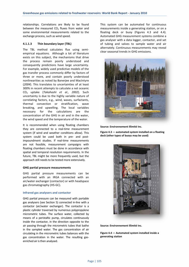
Greenhouse gas emissions related to freshwater reservoirs: World Bank Report - January 2010
Page | 105
relationships. Correlations are likely to be found between the measured CO2 fluxes from water and some environmental measurements related to the exchange process, such as wind speed.
4.1.1.3 Thin boundary layer (TBL)
The TBL method calculates flux using semi-empirical equations. Although a lot of literature exists on this subject, the mechanisms that drive the process remain poorly understood and consequently predictions have large uncertainty. For example, widely used predictive models of the gas transfer process commonly differ by factors of three or more, and contain poorly understood nonlinearities as noted by Banerjee and MacIntyre (2004). This translates to uncertainties of at least 300% in recent attempts to calculate a net oceanic CO2 uptake (Takahashi et al., 2002). Such uncertainty is due to the highly variable nature of correlating factors, e.g., wind, waves, surfactants, thermal convection or stratification, wave breaking, and upwelling. The local variables necessary for the calculations are the concentration of the GHG in air and in the water, the wind speed and the temperature of the water.
It is recommended when using floating chambers they are connected to a real-time measurement system (if wind and weather conditions allow). This system could be used both in pre- and post- impoundment studies. If real-time measurements are not feasible, measurement campaigns with floating chambers must be done in accordance with spatial and temporal resolution requirements. In the future, TBL might be more frequently used, but the approach still needs to be tested more extensively.
GHG partial pressure measurements
GHG partial pressure measurements can be performed with an IRGA connected with an air/water exchanger (contactor) or with headspace gas chromatography (HS-GC).
Infrared gas analysers and contactor
GHG partial pressure can be measured with portable gas analysers (see Section 5) connected in-line with a contactor (air/water exchanger). The contactor is a plastic cylinder traversed by numerous polypropylene micrometric tubes. The surface water, collected by means of a peristaltic pump, circulates continuously inside the contactor, in the direction opposite to the air passing through the micrometric tubes that bathe in the sampled water. The gas concentration of air circulating in the micrometric tubes balances with the gas concentration in the water. The resulting gas-enriched air is then analysed.
This system can be automated for continuous measurements inside a generating station, or on a floating deck or buoy (Figures 4.3 and 4.4). Automated GHG measurement systems combine a gas analyser with a data logger, contactor, and set of tubing and valves to sample water and air alternately. Continuous measurements may reveal clear seasonal trends in GHG emissions.
Source: Environnement Illimité Inc.
Figure 4.3 — automated system installed on a floating deck (other types of buoys may be used)
Source: Environnement Illimité Inc.
Figure 4.4 — Automated system installed inside a generating station
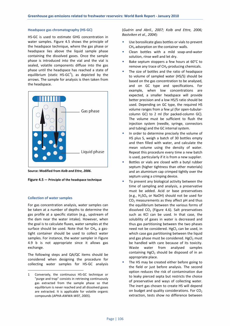
Greenhouse gas emissions related to freshwater reservoirs: World Bank Report - January 2010
Page | 106
Headspace gas chromatography (HS-GC)
HS-GC is used to estimate GHG concentration in water samples. Figure 4.5 shows the principle of the headspace technique, where the gas phase or headspace lies above the liquid sample phase containing the dissolved gases. Once the sample phase is introduced into the vial and the vial is sealed, volatile components diffuse into the gas phase until the headspace has reached a state of equilibrium (static HS-GC1
), as depicted by the arrows. The sample for analysis is then taken from the headspace.
Source: Modified from Kolb and Ettre, 2006.
Figure 4.5 — Principle of the headspace technique
Collection of water samples
For gas concentration analysis, water samples can be taken at a number of depths to determine the gas profile at a specific station (e.g., upstream of the dam near the water intake). However, when the goal is to calculate fluxes, water samples at the surface should be used. Note that for CH4, a gas-tight container should be used to collect water samples. For instance, the water sampler in Figure 4.9 b is not appropriate since it allows gas exchange.
The following steps and QA/QC items should be considered when designing the procedure for collecting water samples for HS-GC analysis
1 Conversely, the continuous HS-GC technique or
"purge and trap" consists in retrieving continuously gas extracted from the sample phase so that equilibrium is never reached and all dissolved gases are extracted. It is applicable for volatile organic compounds (APHA-AWWA-WEF, 2005).
(Guérin and Abril., 2007; Kolb and Ettre, 2006; Bastviken et al., 2004):
• Use borosilicate glass bottles or vials to prevent CH4 adsorption on the container walls.
• Clean bottles with a mild soap-and-water solution, rinse well and let dry.
• Bake septum stoppers a few hours at 60°C to remove any trace of CH4-producing chemicals.
• The size of bottles and the ratio of headspace to volume of sampled water (HS/S) should be based on the gas concentration to be analysed, and on GC type and specifications. For example, when low concentrations are expected, a smaller headspace will provide better precision and a low HS/S ratio should be used. Depending on GC type, the required HS volume ranges from a few μl (for open-tubular-column GC) to 2 ml (for packed-column GC). The volume must be sufficient to flush the injection system (needle, syringe, connectors and tubing) and the GC internal system.
• In order to determine precisely the volume of HS plus S, weigh a batch of 30 bottles empty and then filled with water, and calculate the mean volume using the density of water. Repeat this procedure every time a new batch is used, particularly if it is from a new supplier.
• Bottles or vials are closed with a butyl rubber septum (higher tightness than other materials) and an aluminium cap crimped tightly over the septum using a crimping device.
• To prevent any biological activity between the time of sampling and analysis, a preservative must be added. Acid or base preservatives (e.g., H2SO4 or NaOH) should not be used for CO2 measurements as they affect pH and thus the equilibrium between the various forms of dissolved CO2 (Figure 4.6). Salt preservatives such as KCl can be used. In that case, the solubility of gases in water is decreased and thus gas partitioning between the two phases need not be considered. HgCl2 can be used, in which case gas partitioning between the liquid and gas phase must be considered. HgCl2 must be handled with care because of its toxicity. Waste water from analysed samples containing HgCl2 should be disposed of in an appropriate place.
• The HS may be created either before going to the field or just before analysis. The second option reduces the risk of contamination due to leaky pierced septa but restricts the choice of preservative and ways of collecting water. The inert gas chosen to create HS will depend on budget and quality considerations. For CO2 extraction, tests show no difference between

Greenhouse gas emissions related to freshwater reservoirs: World Bank Report - January 2010
Page | 107
nitrogen and argon, but argon would be more suitable for CH4 extraction (Lambert and Fréchette, 2005). Helium is more expensive but is suitable for CO2 and CH4 extraction. The use of glass instead of plastic syringes reduces the risk of leaks, but increases the cost.
Creating HS before going to the field
• In the lab, use a solid preservative such as KCl (use a sufficient quantity to reach saturation).
• Install the septum and an aluminium cap with a crimping device.
• Weigh the bottles with preservative, septum and aluminium cap.
• Evacuate bottles thoroughly using a good electrical vacuum pump (note that no vacuum is perfect; a small amount of air always remains).
• Collect a certain amount of inert gas (based on the desired HS/S ratio) using a syringe and needle, and insert the needle into the septum of the sample bottle.
• In the field, collect water samples by inserting a needle through the septum in the water. Keep the bottle in the water until it is full (less HS). The remaining HS should have nearly the same volume as the inert gas inserted.
• Note the water temperature and atmospheric pressure for partitioning of gas between the water and gas phase during calculations.
• Place the bottles upside down to reduce leaks from the pierced septum.
• Store in a cool, dark place (e.g., in a cooler).
Creating HS just before analysis
• In the field, fill bottles completely with sampled water taking care not to produce any gas bubbles.
• Install the septum and an aluminium cap with a crimping device.
• Insert a liquid preservative using a syringe and needle (inserted so it is near the bottom of the bottle). Evacuate surplus water using a second needle (inserted near the surface so that the preservative is not evacuated). The amount of liquid preservative should be small enough not to affect significantly the water sample volume. KCl solution must not be used since it would significantly dilute the sampled water.
• Note the water temperature and atmospheric pressure for partitioning of gas between the water and gas phase during calculations.
• Store in a cool, dark place (e.g., in a cooler) until processed in the lab.
• In the lab, weigh filled bottles. • Collect a certain amount of inert gas (based on
the desired HS/S ratio) using a syringe (glass is better than plastic to prevent leakage) and needle, and insert the needle into the septum of the water sample, held upside down. Insert a second needle to evacuate surplus water.
• Reweigh the bottle. The volume of HS and S are calculated based on the difference in weight between the completely filled bottle and the bottle with HS.
• Store the bottle upside down to prevent leakage from the pierced septum.
HS-GC analysis
HS-GC theory and practice are covered by many reference manuals (e.g., Kolb and Ettre 2006). Specialised laboratories or universities can perform HS-GC analysis. The sample preparation steps to perform are as follows (for details, see Kampbell and Vandegrift, 1998):
• Calibrate the gas chromatographer with the gas standard.
• Let the samples reach room temperature. • Shake the samples on a rotary shaker for
five minutes. • Inject the samples into the gas chromatographer.
Source: Wetzel, 2001
Figure 4.6 — CO2 dissolved forms
Correction of HS-GC results for partitioning between the water and gas phase
Results from HS-GC analyses of water samples must be corrected for the HS/S partitioning of gases unless a salt preservative is used. Salt preservatives such as KCl decrease gas solubility and gases are thus mostly found in the HS. The difference between the gas partial pressure in water (pGas) and gas partial pressure measured by HS-GC are a function of gas solubility (K0), gas partial pressure in the HS before equilibrium

Greenhouse gas emissions related to freshwater reservoirs: World Bank Report - January 2010
Page | 108
(pInitial: correspond to the inert gas plus a certain amount of air not evacuated) and after equilibrium
(pFinal: correspond to a mixture of gases), molar volume (Vm) and HS/S ratio:
Sample
m
InitialFinalemEquilibriuFinal
KV
ppS
HSKppGas
0
0 ))(*)(()*( −+
=
where K0 Sample is gas solubility at the sampling temperature; K0 Equilibrium is gas solubility at the equilibrium temperature, just before analysis. Partitions of CO2 and CH4 are calculated using:
))100T(*0.0050578+)
100T(*0.025888-(0.027766*S
+)100Tln(*22.294+)
T100(*90.5069+-58.0931)(ln
2KK
K
K20 =COK
)100T(*6.1698-)
100Tln(*65.2553
)100/(T155.5756+-115.6477)(ln KK
K40 +=CHK
where TK is the temperature in degrees Kelvin, K0(CO2) is CO2 solubility in mole.L-1.atm-1 (Weiss, 1974), S is the salinity in parts per thousands and K0(CH4) is the CH4 solubility in molar fraction.atm-1 (Lide, 2007). Solubility in
molar fraction.atm-1 is multiply by
)weight]molecular [water g/mole 18.0153
density][water g/L 000,1( to obtain a solubility in mole.L-1.atm-1.
The molar volume is calculated using:
)325.101(*)15.273(*082057.0*1P
TP
nRTV Km +==
where n is the number of moles, R is the perfect gas constant (in L.atm.K-1.mol-1), P is the atmospheric pressure (in atmospheres), TK is the temperature in Kelvin and T is the temperature in degrees Celsius
.
Wind speed measurements
Wind speed can be measured on site with a portable anemometer or at a nearby meteorological station.
WMO (2008) – No. 8, Part I - Chapter 5: Wind speed should be reported to a resolution of 0.5 m s–1 or in knots (0.515 m s–1) to the nearest unit, and should represent, for synoptic reports, an average over 10 min. Surface wind is usually measured by a wind vane and cup or propeller anemometer. For nearly all applications, it is necessary to measure the averages of wind speed and direction. Many applications also need gustiness data. A wind-measuring system, therefore, consists not only of a sensor, but also of a processing and recording
system. Simple hand-held anemometers, if they are used, should be set up and read in accordance with the maker’s instructions.
Water temperature
APHA-AWWA-WEF (2005) – Standard Methods 2550: Laboratory and other non-depth temperature measurements should normally be made with any good mercury-filled Celsius thermometer. As a minimum, the thermometer should have a scale marked for every 0.1°C. Depth temperature measurements required for limnological studies may be measured with a reversing thermometer, thermophone, or thermistor. The thermistor is most convenient and accurate; however, higher cost may preclude its Us.

Greenhouse gas emissions related to freshwater reservoirs: World Bank Report - January 2010
Page | 109
Flux calculations
Diffusive flux of gas across the thin boundary layer (TBL) can be calculated from the following equation:
)( airwaterx CCkFlux −= MacIntyre et al., 1995
Where Flux is expressed in mmol of CO2 or µmol CH4 m-2 d-1.
Cair is the concentration of gas in the air
Cwater is the concentration of gas in the water (obtained by the product of gas partial pressure (pGas) times the gas solubility (K0) at a given temperature) obtained with:
][*].atmL.[ ]L.mole[ -1-10
-1 atmpGasmoleKCwater µµ = Morel, 1982; Anderson, 2002
))100T(*0.0050578+)
100T(*0.025888-(0.027766*S
+)100Tln(*22.294+)
T100(*90.5069+-58.0931)(ln
2KK
K
K20 =COK
Weiss, 1974
where K0 (CO2) is the solubility of CO2 in water expressed in mole L-1 atm-1, TK is the temperature in Kelvin, and S is the salinity in parts per thousands. Hence, in freshwater systems, only the first part of the equation is necessary as S = 0.
)100T(*6.1698-)
100Tln(*65.2553
)100/(T155.5756+-115.6477)(ln KK
K40 +=CHK Lide, 2007
where K0 (CH4) is the solubility of CH4 in mole fraction atm-1 and TK is the temperature in Kelvin. Multiply by
)g/mole 18.0153g/L 1000( to obtain a solubility in mole L-1 atm-1.
and with:
xx
Sckk −= )600
(600
where kx is the gas exchange coefficient expressed in cm h-1, x is equal to 0.66 for wind speed ≤ 3 m s-1 and is equal to 0.5 for wind speed > 3 m s-1, and Sc is the Schmidt number for CO2 or CH4 which is dependent on temperature (t):
32
2 04132.04527.3118.11-1911.1)( tttCOSc −+= Wanninkhof, 1992
32
4 039061.02902.3114.28-1897.8)( tttCHSc −+= Wanninkhof, 1992
and:
)215.0(07.2 7.110600 Uk ×+= Cole and Caraco, 1998
64.1
10600 45.0 Uk ×= MacIntyre et al., 1995
)228.0(68.1 2.210600 Uk ×+= Crusius and Wanninkhof, 2003
where k600 is the gas exchange coefficient expressed in cm h-1 normalised for CO2 at 20ºC in fresh water with a Schmidt number of 600. Various k600 equations exist in the literature and were developed for specific study sites or region.
and: 110 22.1 UU ×=

Greenhouse gas emissions related to freshwater reservoirs: World Bank Report - January 2010
Page | 110
where U1 is the wind speed at the water surface and U10 is the frictionless wind speed at 10 m expressed in m s-1 (Crusius and Wanninkhof, 2003).
The resulting final number should be multiplied by 0.24 or
)1000
110000124
cm 10001L( 2
2
3 molemmole
mcm
dh
µ××× to obtain a flux in mmole m-2 d-1. Then, multiply by
44.0098 g mole-1 to obtain a flux in mg CO2 m-2 d-1 or multiply by 16.04276 g mole-1 to obtain a flux in mg CH4 m
-2 d-1
4.1.2 Bubbling – Measurements using funnels
The gases generated in the reservoir sediment are initially dissolved in the interstitial water. The less soluble gases, such as the CH4, aggregate as bubbles that can grow until the point of being liberated and migrate to the water surface. Under deeper depths, bubbles dissolve in the water on their way to the atmosphere. Also, shallow waters, with high oxygen concentration can be a CH4 sink, as the bacteria in these waters can oxidise CH4 to CO2. Bubble fluxes mainly occur in shallow parts of reservoirs where the hydrostatic pressure is not sufficiently high to dissolve CH4 in the interstitial water. Due to discontinuity of ebullition it is important to extend the collection time over days. This process can be important in regions where peatland is impounded. Ebullition is known to be an important pathway for CH4 emissions in many peatlands (Christensen et al., 2003). It can be important in warm and shallow water with OM, but it is only relevant in waters up to 10 m depth (or, according to conservative criteria, up to 20-30 m depth). This implies that the bathymetry of the reservoir has to be considered when extrapolating the measurements, as only shallow zones need to be taken into consideration. No bubbling occurs in the drawdown zone of the reservoir, because water level fluctuation coupled with wave action, results in the organic sediments being completely eroded away and the OM is no longer present.
Open floating dynamic chambers have been used to measure bubble emission (Ramos et al., 2006). Ebullition and diffusive fluxes can be estimated separately using the distribution and variance in apparent piston velocities (k600) from various fluxes obtained from floating chambers (Bastviken et al., 2004). Acoustic techniques have also been used to quantify bubbles (Ostrovsky, 2003; McGinnis et al. 2006; Ostrovsky et al., 2008). The most frequently used methods for measuring bubbling employ inverted funnels coupled to gas collectors initially filled with water, which capture the ascending
bubbles. Bubble collectors installed below wind-wave influence can be used to integrate bubble emission over time and are cheap and easy to operate.
Samples are collected using a set of funnel collectors. If the environment is believed to emit small amounts of bubbles, large bubble collectors should be installed for longer periods of time to maximize potential bubble collection. In most cases, the funnels are placed along transects from the shallows to the deepest regions. The funnels are submersed and all air is removed to avoid contamination by atmospheric air. The collecting bottles, full of water, are then coupled to the funnels. The choice of sampling site and the arrangement of funnels are determined by variables such as the density of flooded vegetation, number of years since impoundment, depth, presence of semi-submerged vegetation, soil/sediment composition and geographic region of the reservoir. The water flow should be near zero and the bottom slope should be less than 20 deg. in order for the system to remain stable over a long period of time.
4.1.2.1 Funnel design
Below is the list of materials required to build funnels. This list is given as an example; other designs may be used. However, it is important to realise, that the material chosen for the funnel and gas-collection bottle will affect the sampling interval. CH4 can diffuse through plastic so, if that material is used, the sampling interval must not exceed 24 hours. Gas can be sampled over longer intervals if a glass bottle is used.
Example of materials required to build funnels for windy conditions (large waves):
• 1 aluminium ring, 1 m diameter • PVC canvas • 6 steel wires (clothes line), 1.2 m long • 2 steel rings, 40 mm • 12 cable screws • 1 lead weight, 2.5 kg

Greenhouse gas emissions related to freshwater reservoirs: World Bank Report - January 2010
Page | 111
• 2 eye bolts, 50 mm • 4 repair links • 1 plumbing collar • 1 swivel • ABS tubing and fittings, 50 mm • syringe with 2-way valve, 150 ml • 1 toilet check valve • 1 bungee cord, 1 m long • 1 buoy, 300 mm diameter • 1 anchor • rope
The PVC canvas is sewed into a funnel shape and fixed onto the aluminium ring. The ABS tubing and fittings are tied to the small end of the funnel using the collar. The syringe fits perfectly into the tube thread and the check valve is use as a gasket. The fittings are arranged so that the syringe is always protected and easy to install or retrieve. The funnel is installed mouth down and is held in place by six steel wires. The top wires are tied to the buoy with a bungee cord and secured with a rope. A lead weight is attached to the end of the bottom wires to keep the funnel upright in the water. A swivel is installed between the lead weight and the anchor line to prevent the system from twisting. This design absorbs the effect of waves on the buoy, but must be used in water at least 3 m deep because of its length (Figure 4.7).
A simpler system for areas where very high bubbling is expected or with little or no wind and wave action consists of a simple funnel with a septum at the narrow end. The gas is thus stored inside the funnel rather than in a syringe (small volume). This design is shorter and can be installed in shallower, calm areas (no wind and waves). The angle of the funnel may be adjusted in either design, depending on water turbulence and waves. Larger angles can be used in calm waters.
4.1.2.2 Collecting gas from funnels
The collection period may last from 24 hours to several days, weeks or the whole season, with intermittent sampling. If a syringe is used to collect gas, the volume of gas collected should be noted before introducing gas into subsample vials or gasometers. If a funnel with a septum is used, all of the gas should be retrieved and the total volume noted. The collection bottles must be hermetically sealed while still under water and are collected for later laboratory analysis.
If a portable GC analyser is used, gas samples can be collected with plastic syringes and analysed the same day. If analyses are expected to be made more than 12 hours after collection, gas samples should be collected in evacuated borosilicate vials or with a gasometer. Borosilicate vials are much cheaper to use but contamination may occur during handling due to needles and though perforated septa. One way to reduced contamination is to introduce a small quantity of saturated saltwater in the evacuated vial and store the vial upside down.
4.1.2.3 Calculating bubbling fluxes
Gas concentration, sampling interval and funnel area are required to compute bubbling fluxes. Gas concentration in ppm measured with GC can be converted into concentration in mg m-3. If the sampling interval is 12 hours or less, atmospheric pressure (AtmP) and water temperature (T) can be measured and used in the concentration conversion calculation. For longer sampling intervals, mean water temperature and atmospheric pressure can be used. If the atmospheric pressure was not recorded, a standard atmospheric pressure of 101.325 kPa can be used.
C])T[(273.13K*.mole8.3144J.K][*].[*].[].[. 1-1-
13
+=
−− KPaAtmPmolegeightMolecularWppmGasConcmmgGasConc
Bubbling fluxes can be calculated using:
][*][][.*]..[]..[ 2
3312
daystervalSamplingInmFunnelAreamCollectedGasVolmmgGasConcdmmguxesBubblingFl
−−− =
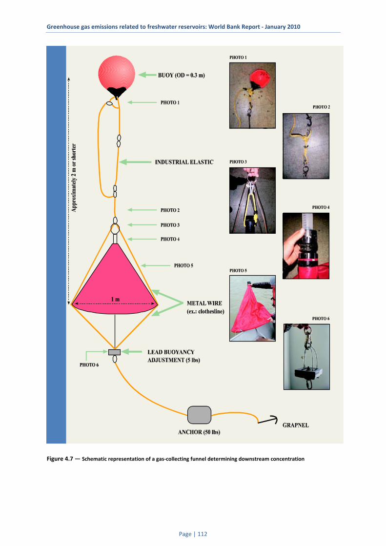
Greenhouse gas emissions related to freshwater reservoirs: World Bank Report - January 2010
Page | 112
Figure 4.7 — Schematic representation of a gas-collecting funnel determining downstream concentration

Greenhouse gas emissions related to freshwater reservoirs: World Bank Report - January 2010
Page | 113
4.1.3 Downstream emissions
Downstream emissions are those observed below reservoir outlets (turbines, spillways, low-level outlets, etc.). They are composed of degassing and diffusive fluxes, and their influence may range from a few tens of metres up to 50 km downstream in the river (Abril et al., 2005).
4.1.3.1 Degassing
Degassing is defined as an emission which happens on discharge from low level outlets, including turbine tailwater (induced by dramatic pressure change). A wide variation in the importance of degassing has been reported (1% to 90% of total emissions), and it is influenced by dam design. Degassing downstream of a dam and spillway can be estimated by the difference between the gas concentration upstream (or in the turbine) and downstream of the power plant multiplied by the outlet discharge (see below for calculation).
Determining upstream concentration at or near the water intake
To accurately determine degassing, samples of water entering the turbines must be taken directly at the turbines or at the powerhouse intake. If possible, the gas concentrations should be sampled from ports within the conduits leading to the outlets. If that is not feasible, degassing may be evaluated from the average GHG concentration across vertical profiles in the reservoir if there is no stratification, or by the concentration at the depth of the water intake if there is stratification.
Water profiling of temperature, oxygen and dissolved gas should be performed upstream of the dam to determine whether there is stratification of the water column near the intake. Temperature and oxygen profiles are easy and cheap to measure and help detect any stratification. Once those profiles are measured, gas partial pressure profiles can be obtained using in situ sensors or by collecting water samples at various depths. If water samples are collected, CH4 and CO2 concentrations can be determined by the headspace method followed by gas chromatography analysis (see Section 4.1.1.3 – Gas partial pressure measurements – Headspace gas chromatography).The concentration in water after passing through the turbine and spillway can be determined in water samples taken outside the area of turbulence just downstream of the dam. Water sample GHG concentrations can be determined by the headspace method followed by gas
chromatography analysis (see Section 4.1.1.3 – Gas partial pressure measurements – Headpsace gas chromatography).
Determining water discharge
WMO (1994) – No. 168, Chapter 11: River discharge, which is expressed as volume per unit time, is the rate at which water flows through a cross-section. Discharge at a given time can be measured by several methods, the choice of which depends on the conditions encountered at a particular site. A number of approaches are outlined below.
• Measurement of discharge by current meters: general steps include selection of sites, measurement of cross-sections, measurement of velocity, and computation of discharge.
• Measurement of discharge by the float method: general steps include selection of sections, selection and installation of floats, measuring procedure, computation of velocity, and computation of discharge.
• Measurement of discharge by dilution methods: general steps include selection of site, tracers and detection equipment, and computation of discharge.
• Measurement of corresponding stage: stage and corresponding time are noted at intervals to identify segments of total discharge with time and stage.
• Computations of discharge by indirect methods: the peak discharge may be determined after the flood has subsided by computations that combine well-established hydraulic principles with field observations of channel conditions and flood profiles. All of the methods involve the simultaneous solution of continuity-of-mass and energy equations. Such computations may be made for reaches of a river channel, through roadway culverts and bridge openings, and over dams and highway embankments. Although the hydraulic formulae differ for each type of waterway, all of the methods involve the following factors: geometry and physical characteristics of
the channel and boundary conditions of the reach used;
water surface elevations at the time of peak stage to define the cross-sectional areas and the head difference between two significant points;
hydraulic factors, such as roughness coef-ficients based on physical characteristics.

Greenhouse gas emissions related to freshwater reservoirs: World Bank Report - January 2010
Page | 114
• Measurement of discharge under difficult conditions: such conditions include unstable channels, mountain streams, or measurement of unsteady flow.
• Non-traditional methods of stream gauging: moving-boat method, ultrasonic (acoustic) method, electromagnetic method.
Calculating degassing
The degassing flux ( gDegasFlux sin ) is calculated as follow:
))][](([))][](([sin SdownsSUpSTdownsTUpTgDegas QGasGasQGasGasFlux ×−+×−=
where UpTGas][ is the gas (CH4 or CO2) concentration upstream of the generating station (turbines) expressed
in mg/m3, downsTGas][ is the gas concentration downstream of the generating station, TQ is the turbine
flow and ,][ UpSGas ,][ downsSGas and SQ are equivalent terms for the spillway.
The flow should be for the same time period as gas concentration measurements. The best-case scenario would entail continuous gas concentration measurements (e.g., every three hours), averaging concentrations for each day and calculating using the mean daily flow (turbine and spillway). If the operating mode (peaking) is expected to vary on an hourly basis, it may then be useful to calculate degassing fluxes for every hour. The gas concentration sampling interval should thus be determined on the basis of the operating mode.
4.1.3.2 Fluxes in the downstream aquatic system
Diffusive and bubbling fluxes should be measured in the aquatic system downstream of the (proposed or existing) dam up to a maximum distance of 50 km. This distance may vary from site to site and must be assessed for each project. Comparison of emissions in the aquatic system downstream of the dam before and after impoundment will indicate whether leakage from the reservoir affects the downstream ecosystem. The methods described in Section 4.1.1 and 4.1.2 can be used.
4.2 Carbon stock Carbon content in water should be measured at representative stages in stream hydrographs and, when combined with discharge calculations, allow carbon transport to be determined. Carbon stock in the water column and in sediment should be determined as described below.
4.2.1 Carbon availability in water column / transport
Carbon present in the water column is subject to transport downstream from the reservoir. The evaluation of the carbon stock present in the area to
be flooded by the reservoir is a critical measurement, as it can be used as an indicator of future reservoir GHG emissions, GHG emissions being proportional to the content in organic matter flooded.
Most lakes are supersaturated in CO2 (Del Giorgio et al., 1999), and thus generally emit CO2 to the atmosphere. CO2 saturation is linked to the dissolved organic carbon (DOC) concentration (Bird and Prairie, 2003). DOC is degraded by various processes including biological degradation and photo-oxidation into dissolved inorganic carbon (DIC).
Organic matter is composed of particulate and dissolved organic carbon (POC, DOC) and organic compounds containing sulphur (S), nitrogen (N) and phosphorus (P). Carbon (C) in a water body can be in particulate or dissolved form, and can be organic and inorganic. Below is a description of the processes producing DOM, TOC, DOC, TIC and DIC.
4.2.1.1 Dissolved organic matter (DOM)
DOM can be of autochthonous or allochthonous origin. Autochthonous DOM in aquatic ecosystems is produced by photosynthesis (Häder, 1997), extracellular release and exudation mechanisms, or by the degradation of plankton and macrophytes (e.g., mortality, grazing, biodegradation, photodegradation) (Obernosterer et al., 1999). Allochthonous DOM, by contrast,

Greenhouse gas emissions related to freshwater reservoirs: World Bank Report - January 2010
Page | 115
originates from terrestrial input from the catchment (Hessen, 2002). The proportion of allochthonous and autochthonous DOM is influenced by the degree of aquatic productivity, precipitation, terrestrial inputs and elevation (Williamson et al., 1996).
The majority (> 50%) of freshwater DOM (Corin et al., 1996; Ertel 1990; Herndl et al., 1997; Wetzel et al., 1995; Davies-Colley and Vant, 1987; Reche et al., 1999; Moran and Hodson, 1990) is composed of dissolved humic substances (DHS). Dissolved humic substances are dark coloured, acidic and composed primarily of aromatic molecules (Gastonguay et al., 1995) originating from terrestrial plant material.
4.2.1.2 Total organic carbon (TOC)
TOC is the quantity of carbon present in the organic matter which is dissolved (DOC) or suspended (POC) in water.
4.2.1.3 Dissolved organic carbon (DOC)
Decomposition of DOC is ten times greater than that of POC and is, additionally, accelerated by photolysis and its subsequent bioavailability, contributing to the efflux of CO2 to the atmosphere (Wetzel et al., 1995).
4.2.1.4 Dissolved inorganic carbon (DIC)
DIC is also referred to as total inorganic carbon (TIC). DIC represents the total of the three CO2 aqueous forms: HCO3
-, CO32- and free CO2. The
equilibrium between these three CO2 forms depends on pH. DOC is transformed into DIC by
photo-oxidation (Ertel, 1990; Petterson et al., 1997; Dahlen et al., 1996; Vodacek et al., 1997) and micro-organism respiration (Cole, 1999).
The origin of DOM influences the formation of DIC. Lakes with high primary production (high chlorophyll concentrations and high concentration of autochthonous DOM) produce less DIC (Bertilsson and Tranvik 2000). Therefore, DOC will be more easily mineralised into DIC in humic oligotrophic lakes than in eutrophic lakes with high algal productivity and where photosynthesis rates are high (carbon acquisition).
DIC production at the sediment/water interface is influenced by the water oxygen-content, which affects the rate of methane consumption by methanotrophic bacteria producing CO2.
4.2.1.5 C:N:P ratio
Elemental chemical composition of planktonic particulate organic matter reflects the planktonic structure as well as biochemical processes (Table 4.2). Phosphorus (P), and to a lesser extent nitrogen (N), are limiting elements for freshwater plant productivity. Limitation in these elements can lead to alteration in cell content and to the C:N ratio. The carbon content of organic matter is on average at least an order of magnitude greater than that of nitrogen (N). The C:N ratio for allochthonous DOM varies from 45:1 to 50:1 and for autochthonous DOM it is 12:1 (Wetzel 2001). The majority of N is proteinaceous in the plankton.
Table 4.2 — Type of organic matter and C:N:P ratio
Source: Wetzel, 2001.
Determination of the trophic state (autotroph vs. heterotroph) of a water body can be based on its content in total nitrogen (TN) and total phosphorus (TP; Figure 4.8). Primary productivity,
phytoplankton density and biomass, chlorophyll a, dominant phytoplankton, light extinction coefficient, TOC and total inorganic solids are other characteristics of trophic status (Wetzel, 2001).
Type of organic matter C:N:P ratioAllochthonous DOM C:N varies from 45:1 to 50:1Autochthonous DOM C:N ~ 12:1
Streams, shallow lakes, reservoirs with short residence times C:P < 350 N:P < 26
Streams, shallow lakes, reservoirs with residence times > 6 months C:P > 400 N:P > 30
Tropical lakes high C:N

Greenhouse gas emissions related to freshwater reservoirs: World Bank Report - January 2010
Page | 116
Data are shown as an example. Graph based on Wetzel’s (2001) relationship of lake productivity to N and P concentrations.
Figure 4.8 — Trophic state determination based on TN and TP
4.2.1.6 Origin of organic matter – ∂13C analysis
The origin of organic matter can be assessed by ∂13C analysis (Hélie, 2004). There are three isotopes of carbon: 12C, 13C and 14C (in order of importance). Plants use two types of atmospheric carbon during photosynthesis: 12C and 13C. Various 12C:13C ratios are founded in plants depending on plant types (C3 vs. C4: mainly grass and sedge families). If terrestrial plants use air CO2, which has a mean ∂ 13C value of -8‰, aquatic plants use dissolved CO2, which has more variable ∂ 13C. The use of ∂ 13C-OM signatures to identify aquatic against terrestrial production is largely site specific. However, in most cases it provides a relatively sensitive indicator of their ratio in riverine OM fluxes (Rau, 1978; Barth, 1998).
4.2.1.7 Collection of samples in the water column
In order to estimate the carbon stock in the water column, water samples must be collected from various depth increments using a water sampler (Figure 4.9). Types of samples include (WMO, 1994):
• Grab samples. These are used to characterise water quality at a particular time, location and depth. Grab samplers may be categorised into those appropriate for non-volatile constituents and those suitable for dissolved gases. Van Dorn bottles, Kemmerer samplers and (diaphragm, peristaltic or rotary) pumps may be used for DOC sampling.
• Composite samples. These are obtained by mixing several discrete samples of equal volume. Composite samples provide average water quality conditions over the time of sampling. It is more economical since fewer samples are required. There are two types of composite samples: sequential (i.e., at a regular time interval) andflow-proportional.
Source: Somer, 1992 –above; WMO, 1994 –following page
Figure 4.9 — Water sampler-integrator
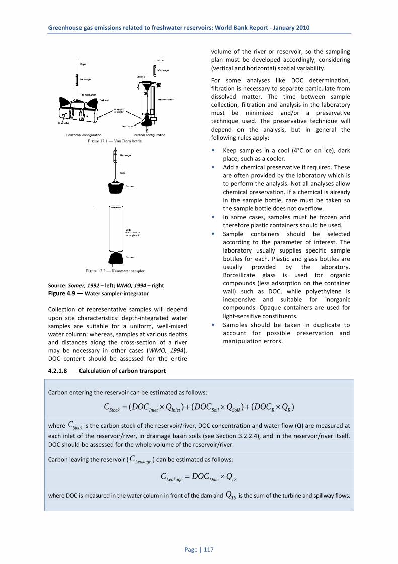
Greenhouse gas emissions related to freshwater reservoirs: World Bank Report - January 2010
Page | 117
Source: Somer, 1992 – left; WMO, 1994 – right Figure 4.9 — Water sampler-integrator
Collection of representative samples will depend upon site characteristics: depth-integrated water samples are suitable for a uniform, well-mixed water column; whereas, samples at various depths and distances along the cross-section of a river may be necessary in other cases (WMO, 1994). DOC content should be assessed for the entire
volume of the river or reservoir, so the sampling plan must be developed accordingly, considering (vertical and horizontal) spatial variability.
For some analyses like DOC determination, filtration is necessary to separate particulate from dissolved matter. The time between sample collection, filtration and analysis in the laboratory must be minimized and/or a preservative technique used. The preservative technique will depend on the analysis, but in general the following rules apply:
• Keep samples in a cool (4°C or on ice), dark place, such as a cooler.
• Add a chemical preservative if required. These are often provided by the laboratory which is to perform the analysis. Not all analyses allow chemical preservation. If a chemical is already in the sample bottle, care must be taken so the sample bottle does not overflow.
• In some cases, samples must be frozen and therefore plastic containers should be used.
• Sample containers should be selected according to the parameter of interest. The laboratory usually supplies specific sample bottles for each. Plastic and glass bottles are usually provided by the laboratory. Borosilicate glass is used for organic compounds (less adsorption on the container wall) such as DOC, while polyethylene is inexpensive and suitable for inorganic compounds. Opaque containers are used for light-sensitive constituents.
• Samples should be taken in duplicate to account for possible preservation and manipulation errors.
4.2.1.8 Calculation of carbon transport
Carbon entering the reservoir can be estimated as follows:
)()()( RRSoilSoilInletInletStock QDOCQDOCQDOCC ×+×+×=
where StockC is the carbon stock of the reservoir/river, DOC concentration and water flow (Q) are measured at
each inlet of the reservoir/river, in drainage basin soils (see Section 3.2.2.4), and in the reservoir/river itself. DOC should be assessed for the whole volume of the reservoir/river.
Carbon leaving the reservoir ( LeakageC ) can be estimated as follows:
TSDamLeakage QDOCC ×=
where DOC is measured in the water column in front of the dam and TSQ is the sum of the turbine and spillway flows.
Greenhouse gas emissions related to freshwater reservoirs: World Bank Report - January 2010
Page | 118
4.2.2 Carbon storage in sediments
Methane (CH4) and nitrous oxide (N2O) are produced by bacteria living in the sediments: anaerobic methanogenic bacteria, and nitrifying and denitrifying bacteria, respectively (Eriksson III et al., 2000; Schmidt and Conrad, 1993; Svensson, 1998; Bastien, 2005).
POC is the dominant source of organic matter in sediments; some DOC may be incorporated into the sediments by adsorption on clays and carbonate (Dean, 1999) or by flocculation with other particulates in the water column (Simon et al., 2002; Wetzel, 2003). This carbon is stored in three main components of lake sediments: organic matter, autogenic carbonate minerals and non-carbonate mineral detritus (Dean, 1974; Wetzel, 1975). Sediment is made up of a complex mixture of lipids, carbohydrates, proteins and other biochemicals contained in the tissues of living benthic micro-organisms, and the detritus of organisms formerly living in the lake and its catchment (Meyers and Ishiwatari, 1993).
Bacterial activity, carbon oxidation (degradation process), bioturbation and resuspension of sediment that occur at the water/sediment interface (active layer) affect the carbon storage estimation in sediment surface layers (Meyers and Ishiwatari, 1993).
Once buried below the zone of bioturbation, organic matter is subject to further bacterial degradation, often resulting in methanogenesis. Only less reactive forms of organic matter accumulate in the sediments. Under that “active zone,” most of the sediment carbon is permanently buried and not involved in the biogeochemical processes (Sobek et al., 2006).
Carbon in sediment is mainly found in the form of particulate organic carbon (POC). The International Organization for Standardization (ISO) provides guidance on sampling of bottom sediments (Appendix 1 – International Organization for Standardization, Guidance and Sampling Procedures, ISO 5667-12:1995). Sediment samples can also be collected as described in Environnement Canada (2002 a and b; Appendix 1 – Sediment Sampling Guide for Dredging and Marine Engineering Projects in the St. Lawrence River. Volumes 1 and 2). The choice of sampling method must consider hoisting equipment
available, physical constraints of the environment (e.g., bathymetry, currents and waves), the penetration depth required, sample integrity, the type of material used to make the sampler (plastic should not be used for organic analyses) and the sample volume required (Environment Canada, 2002 a and b; Figure 4.10).
Sediments
• Grab samplers. Samplers equipped with a set of jaws and suitable for high-volume sampling of homogenous sediment. Grab sampler types include Ekman, Ponar, Van Veen, Shipek, Smith-McIntyre and US BM54 samplers.
• Corers. Tubes sunk into the sediment by various means to obtain a core of known length. Corers usually make it possible to characterise the entire depth of sediment and to obtain unmixed sediment samples. Corer types include: Hand/mechanical corers – deployed by a
diver or a rod (piston) Gravity corers – open-barrel or piston-
/cable-operated Vibratory corers
• Subsampling of cores or grab sampling must be carried out for subsequent laboratory analysis.
• Pore water fills the interstices between sediment particles. In general, concentrations of different substances tend to reach an equilibrium between pore water and sediment (Environment Canada, 2002 b). Pore water can be used to assess the mobility of carbon from the sediment into the water column. However, pore water extraction methods usually affect DOC content. Direct methods dialysis. (may be used to extract
dissolved gas); direct suction.
Indirect methods centrifuging, squeezing.
Detailed sampling methods, sample acceptability criteria, sample manipulation and conservation methods are described in Appendix 1 – Sediment Sampling Guide for Dredging and Marine Engineering Projects in the St. Lawrence River. Volume 2, Field Operations Manual.
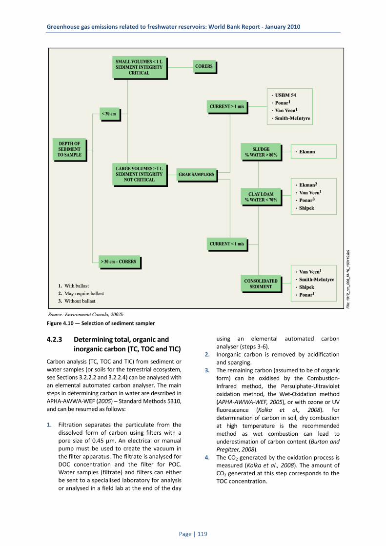
Greenhouse gas emissions related to freshwater reservoirs: World Bank Report - January 2010
Page | 119
Figure 4.10 — Selection of sediment sampler
4.2.3 Determining total, organic and inorganic carbon (TC, TOC and TIC)
Carbon analysis (TC, TOC and TIC) from sediment or water samples (or soils for the terrestrial ecosystem, see Sections 3.2.2.2 and 3.2.2.4) can be analysed with an elemental automated carbon analyser. The main steps in determining carbon in water are described in APHA-AWWA-WEF (2005) – Standard Methods 5310, and can be resumed as follows:
1. Filtration separates the particulate from the dissolved form of carbon using filters with a pore size of 0.45 μm. An electrical or manual pump must be used to create the vacuum in the filter apparatus. The filtrate is analysed for DOC concentration and the filter for POC. Water samples (filtrate) and filters can either be sent to a specialised laboratory for analysis or analysed in a field lab at the end of the day
using an elemental automated carbon analyser (steps 3-6).
2. Inorganic carbon is removed by acidification and sparging.
3. The remaining carbon (assumed to be of organic form) can be oxidised by the Combustion-Infrared method, the Persulphate-Ultraviolet oxidation method, the Wet-Oxidation method (APHA-AWWA-WEF, 2005), or with ozone or UV fluorescence (Kolka et al., 2008). For determination of carbon in soil, dry combustion at high temperature is the recommended method as wet combustion can lead to underestimation of carbon content (Burton and Pregitzer, 2008).
4. The CO2 generated by the oxidation process is measured (Kolka et al., 2008). The amount of CO2 generated at this step corresponds to the TOC concentration.

Greenhouse gas emissions related to freshwater reservoirs: World Bank Report - January 2010
Page | 120
5. Total carbon (TC) generated at steps 2 (inorganic – TIC) and step 4 (organic – TOC) is recorded by the analyser.
6. TIC concentration is determined by the difference between TC and TOC.
QA/QC items:
• Many kinds of filters may be used but it is important that they do not release any DOC during filtration (Kolka et al., 2008). Filtration for DOC is carried out with a glass-fibre filter (to reduce adsorption of DOC on the filter) or with a metal membrane during or immediately after sample collection (WMO, 1994).
• The filter and filter apparatus should be washed with the sample water by discarding the first 200 ml of filtrate.
• All traces of acid must be removed from the samples by complete drying to avoid interference with the analyser’s infrared detector.
5 Gas analysers and gas measurement technologies
5.1 Gas chromatography (GC) analysis
Gas chromatography can be used to analyse dissolved gas in water using the headspace technique as briefly describe in Section 4.1.1.3 or simply for analysing gas in air samples such as those collected from the soil/low vegetation chamber method (Section 3.1.2.1) or from the aquatic diffusive surface flux chamber method (Section 4.1.1.1). CH4 is analysed with a GC equipped with a flame ionisation detector (GC-FID), CO2 with a thermal conductivity detector (GC-TCD), and N2O with an electron capture detector (GC-ECD). General gas chromatography principles and techniques are described in handbooks such as those by McNair and Miller (2009) and Willard et al. (1988).
5.2 Infrared gas analysers (IRGAs) All such analysers have two main components: a light source and a detector. Open-path analysers have an open path between the detector and light source; whereas in closed-path systems, the light
source and detector are enclosed in a sample chamber or light tube .
Key features for good measurements are pressure and temperature compensation (Hashmonay and Crosson, 2009). Some instruments measure pressure and temperature, and automatically compensate for variations in those variables, while others do not.
The gas analysers or technologies listed below can be used for measurements in both terrestrial and aquatic systems. Appendix 2 lists a number of suppliers and cost estimates. Figure 2.4 presents advantages and constraints of the various technologies. Analyser techniques depend on light source type (mid- to near-infrared) and how the light spectrum is treated (position of filter, mirror types and numbers).
• Non-dispersive infrared (NDIR): The term “non-dispersive” refers to the fact that all of the light passes through the gas sample and is filtered just before the detector.
• Fourier-transformed infrared (FTIR): Measurements of electromagnetic or other types of radiation.
• Tunable diode laser spectroscopy (TDLS): Uses a tunable (adjustable) diode laser source that emits in the mid-infrared spectral region (between 3 and 30 µm).
• Cavity ring down spectroscopy (CRDS): A typical CRDS setup consists of a laser that is used to illuminate an optical cavity, which in its simplest form consists of two highly reflective mirrors.
5.3 Automated systems Automated systems combine a measuring instrument with a programmed data logger to sample at fixed intervals. Continuous measurements may clearly reveal seasonal trends in GHG and ancillary variables. This type of system should be used to the extent possible for both terrestrial and aquatic GHG variable monitoring.
For example, in aquatic ecosystems, continuous measurement of gas partial pressure highlights the importance of seasonal and annual variations (Figure 5.1) and thus on GHG emissions. In boreal reservoirs, the use of automated systems have clearly shown 1) a significant increase of pCO2 under the ice cover, 2) a decrease in pCO2 in spring corresponding to the ice-melting period, and 3) lowest pCO2 in late spring or summer, depending of the ecosystem (Demarty et al., 2009).

Greenhouse gas emissions related to freshwater reservoirs: World Bank Report - January 2010
Page | 121
Source: Hydro-Québec and Environnement Illimité Inc.
Figure 5.1 — pCO2 data collected using a CO2 Analyser and a datalogger at Eastmain-1 Reservoir
6 Ancillary measurements
Certain ancillary variables are not necessary for any GHG measurements and calculations yet represent precious information for a comprehensive
understanding of the trends in GHG emissions. Some of these variables are listed below. Various standard measurement protocols exist from national and international agencies. The International Organization for Standardization (ISO) provides protocols for many of the variables presented below and elsewhere in the manual such as pH, conductivity and TOC (Appendix 1). Other equally good standards may exist elsewhere. Table 6.1 presents a summary of ancillary variables and their role.
Table 6.1 — Summary of ancillary variables and their role
Type Ancillary variable Indication / impactWater quality Dissolved oxygen Indicator of productivity and metabolic state
Biological oxygen demand Indicator of secondary productionChlorophyll a Indicator of primary production and trophic state
Nitrogen and phosphorus Indicator of productivity and trophic stateAmmonia nitrogen (NH3) Indicator of agriculture or urban run-off
Total Kjedahl nitrogen Indicator of productivity and trophic stateNitrites (NO2
- ) and nitrates (NO3- ) Indicator of secondary production (nitrifiers)
Total phosphorus and orthophosphates Indicator of primary production,trophic state and agriculture or urban run-offWater color Indicator of organic carbon content
Water transparency Indicator of organic carbon contentTurbidity Indicator of particulate carbon content available for transport
Suspended solids Indicator of particulate carbon content available for transportConductivity Used to calculate pCO2 using thermodynamic equations
pH Indicator of free CO2 content and used to calculate pCO2 using thermodynamic equationsAlkalinity Used to calculate pCO2 using thermodynamic equations
Physical water variables Water level Affects the drawdown zone (aquatic vs. terrestrial)Sediment discharge Affects the particulate carbon stock
Residence time Affects sedimentation and mineralization ratesWave height Affects measurement of fluxes using a floating chamber
Air temperature Indicator of climate typeRelative humidity Indicator of climate type
Wind direction Indicator of wind speed and turbulence (fetch)Precipitation Affects the leakage of organic material from the river basin to the aquatic system
Atmospheric GHG concentrations Indicator of large scale impacts of reservoir creation

Greenhouse gas emissions related to freshwater reservoirs: World Bank Report - January 2010
Page | 122
6.1 Water quality For water quality variables, samples should be collected with a water sampler-integrator (Figure 4.9) of the photic zone (1 to 10 m). If the depth exceeds 10 m, a bottom sample should also be collected.
6.1.1 Dissolved oxygen
Dissolved oxygen (DO) is used as an indicator of the metabolism of a water body. High DO correlates with systems having high primary productivity (also called “autotrophic systems”); whereas, low DO correlates with a high respiration rate and thus systems having high secondary productivity (also called “heterotrophic systems”).
WMO (1994) – No. 168, Chapter 17: The WMO suggests that the dissolved-oxygen concentrations may be determined directly with a DO meter or by a chemical method, such as Winkler analysis.
APHA-AWWA-WEF (2005) – Standard Method 4500-O: The Winkler, or iodometric method, consists of oxidation of DO by addition of divalent manganese solution, followed by a strong alkali. The iodine obtained is then titrated with a standard solution of thiosulphate. The titration end point can be detected visually, with a starch indicator, or electrometrically, with potentiometric or dead-stop techniques. The free iodine can also be measured directly by simple absorption spectrophotometers. Also, several modifications of the iodometric method are given to minimize the effect of interfering materials.
ASTM (2005) – Standard Test D888-05: Three methods are given: titrimetric procedure – high level, instrumental probe procedure and luminescence-based sensor.
6.1.2 Biological oxygen demand
Biochemical oxygen demand (BOD) measures the amount of oxygen consumed by micro-organisms in decomposing organic matter in stream water. BOD also measures the chemical oxidation of inorganic matter.
WMO (1994) – No. 168, Chapter 17: One of the most commonly used measuring methods is the dilution method; however, manometric techniques may have advantages under certain circumstances. BOD is calculated from the measurement of volumetric dilution of the sample and the difference between the dissolved-oxygen concentrations of the sample before and after a five-day incubation period. The temperature
should be kept at 20°C during that period, and atmospheric oxygen should be kept away from the sample, which is stored in the dark to minimize the effect of photosynthetic action of green plants.
6.1.3 Chlorophyll a
Chlorophyll a is a proxy for the productivity of a water body. Associated with phosphorus or nitrogen concentration, it allows the determination of the trophic state of a water body.
APHA-AWWA-WEF (2005) – Standard Method 10200H: The sample is concentrated by centrifuging or filtering. The pigments are extracted from the plankton concentrate with aqueous acetone and the optical density (absorbance) of the extract is determined with a spectrophotometer or by fluorimetric determination.
6.1.4 Nitrogen and phosphorus
Nitrogen and phosphorus are the major nutrients limiting freshwaters primary production. Associated with chlorophyll a concentration, they allow the determination of the trophic state of a water body.
6.1.4.1 Ammonia nitrogen
APHA-AWWA-WEF (2005) – Standard Method 4500-NH3: This method applies to measurements in drinking and surface waters, and in domestic and industrial wastes. Dissolved ammonia (NH3(aq) and NH4
+) is converted to NH3(aq) by raising pH. NH3(aq) diffuses through the membrane and changes the internal solution pH that is sensed by a pH electrode. The fixed level of chloride in the internal solution is sensed by a chloride ion-selective electrode that serves as the reference electrode.
USEPA (1993) – Method 350.1 Revision 2: This method covers the determination of ammonia in drinking, ground, surface and saline water, and in domestic and industrial wastes. The sample is buffered and distilled into a solution of boric acid. Alkaline phenol and hypochlorite react with ammonia to form indophenol blue, which is proportional to the ammonia concentration. The blue colour formed is intensified with sodium nitroprusside and measured colorimetrically.
ASTM (2008) – Standard Test D1426-08: This standard is an ion-selective electrode method. It is applicable to the determination of ammonia nitrogen in reagent and effluent water. The test method is applicable to surface and industrial water, and to wastewater following distillation.

Greenhouse gas emissions related to freshwater reservoirs: World Bank Report - January 2010
Page | 123
6.1.4.2 Total Kjeldahl nitrogen
APHA-AWWA-WEF (2005) – Standard Method 4500-N org. B: Acid digestion, distillation and determination with a specific electrode. In the presence of H2SO4, potassium sulphate (K2SO4) and a cupric sulphate (CuSO4) catalyst, the amino nitrogen of many organic materials is converted to ammonium. Free ammonia also is converted to ammonium. After addition of a base, the ammonia is distilled from an alkaline medium and absorbed in boric or sulphuric acid. The ammonia may be determined colorimetrically, by an ammonia-selective electrode technique, or by titration with a standard mineral acid.
ASTM (2006) – Standard Test D3590-02: The standard contains the manual digestion/distillation method and the semi-automated colorimetric Bertholt method.
6.1.4.3 Nitrites and nitrates
APHA-AWWA-WEF (2005) – Standard Method 4500-NO3
-: NO3- is reduced almost quantitatively
to nitrite (NO2-). The NO2
- thus produced is determined by the formation of a highly coloured azo dye that is measured colorimetrically.
ASTM (2009) – Standard Test D3867-09: These test methods cover the determination of nitrite nitrogen, nitrate nitrogen, and combined nitrite-nitrate nitrogen in water and wastewater. The following two test methods are given: Test Method A – Automated cadmium reduction and Test Method B – Manual cadmium reduction. These test methods are applicable to surface, saline, waste and ground water.
USEPA (1993) – Method 353.2 Revision 2.0: This method covers the determination of nitrite alone, or nitrite and nitrate combined in drinking, ground and surface water, and in domestic and industrial wastes. A filtered sample is passed through a column containing granulated copper-cadmium to reduce nitrate to nitrite. The nitrite is treated to form a highly coloured azo dye, which is measured colorimetrically.
6.1.4.4 Total phosphorus and orthophosphates
APHA-AWWA-WEF (2005) – Standard Method 4500-P E: Phosphorus analyses entail two general procedural steps: (a) conversion of the phosphorus form of interest to dissolved orthophosphate, and (b) colorimetric determination of dissolved orthophosphate. Filtration through a membrane filter with a pore size of 0.45 m separates dissolved from suspended forms of phosphorus.
USEPA (1993) – Method 365.1 Revision 2.0: This method covers the determination of specified forms of phosphorus in drinking, ground and surface water, and in domestic and industrial wastes. The methods are based on reactions that are specific to the orthophosphate ion. The form measured depends on the prescribed pretreatment of the sample. The most commonly measured forms are total and dissolved phosphorus, and total and dissolved orthophosphate. Reaction with a reagent creates a complex that is reduced by ascorbic acid to an intensely blue-coloured complex. The colour is proportional to the phosphorus concentration and is measured automatically.
6.1.5 Water colour
The water colour is a proxy for the estimation of the organic matter concentration.
WMO (1994) – No. 168, Chapter 17: The true colour is observed after filtration or centrifuging. Colour results from the presence of metallic ions, humus and peat materials, plankton, and industrial wastes. Colour may be obtained by visually comparing standard glass colour disks with tubes filled with the sample.
6.1.6 Water transparency
WMO (1994) – No. 168, Chapter 17: Transparency of water is determined by its colour and turbidity. A measure of transparency can be obtained from the depth in metres at which a 20- to 30-cm disk, called a “Secchi disk”, usually painted in black and white quadrants, disappears when slowly lowered straight down into the water. Standard block letter on white paper is sometimes used instead of the disk.
6.1.7 Turbidity
Turbidity is an optical measurement of suspended solids, such as clay, silt, organic matter, plankton and microscopic organisms, in a water sample.
WMO (1994) – No. 168, Chapter 17: Turbidity can be measured by nephelometric methods and be expressed in nephelometric turbidity units (NTU). Nephelometric methods measure light scattering by suspended particles. Instruments of different design, however, may give different results for the same sample.
APHA-AWWA-WEF (2005) – Standard Method 2130: It was originally measured by the Jackson candle turbidimeter method, but, this method cannot measure under a turbidity of 25 Jackson Turbidity Units (JTU). Thus, for samples under that
Greenhouse gas emissions related to freshwater reservoirs: World Bank Report - January 2010
Page | 124
value, indirect secondary methods had to be used. Today, the electronic nephelometers are the preferred instruments for turbidity measurement.
6.1.8 Suspended solids
APHA-AWWA-WEF (2005) – Standard Method 2540-D: A well-mixed sample is filtered through a weighed standard glass fibre filter and the residue retained on the filter is dried to a constant weight at 103°C to 105°C. The increase in weight of the filter represents the total suspended solids.
6.1.9 Conductivity
U.S. EPA (1982) – Method 120.1: This method is applicable to drinking, surface, and saline water, domestic and industrial wastes and acid rain (atmospheric deposition). The specific conductance of a sample is measured by use of a self-contained conductivity meter, Wheatstone bridge-type, or equivalent. Samples are preferably analysed at 25°C. If not, temperature corrections are made and results reported at 25°C.
6.1.10 pH
Special care must be taken when measuring the pH of water since pH and pCO2 are tightly linked (Figure 4.6). In the field, completely fill the bottle with the water sample and close the bottle under the water surface. The bottle’s gap must be as small as possible to prevent gas from escaping when the electrode is inserted into the bottle and during pH measurement (a cap with septa maintaining a hermetic seal when inserting the electrode would be better).
APHA-AWWA-WEF (2005) – Standard Methods 4500-H+: At a given temperature the intensity of the acidic or basic character of a solution is indicated by pH or hydrogen ion activity. pH can be measured by the electrometric method. The basic principle of electrometric pH measurement is determination of the activity of the hydrogen ions by potentiometric measurement using a standard hydrogen electrode and a reference electrode.
U.S. EPA (1982) – Method 150.2: This method is applicable to drinking, surface, and saline waters, domestic and industrial wastes and acid rain (atmospheric deposition). The pH of a sample is determined electrometrically using either a glass electrode in combination with a reference potential or a combination electrode. Samples should be analysed as soon as possible after collection, preferably in the field at the time of sampling.
6.1.11 Alkalinity
APHA-AWWA-WEF (2005) – Standard Methods 2320: Alkalinity of water is its acid-neutralising capacity. It is the sum of all the titratable bases. Alkalinity of many surface waters is primarily a function of carbonate, bicarbonate, and hydroxide content; therefore it is taken as an indication of the concentration of these constituents. Measures also may include borates, phosphates, silicates, or other bases if these are present. Alkalinity depends on the end-point pH used. pH is needed to determine the inflection points from titration curves and is the rationale for titrating to fix pH end points. The titration curve is constructed by recording sample pH with a pH meter after successive small measured additions of titrant to identify inflection points and buffering capacity. For more information, refer to the complete method.
6.2 Physical water variables
6.2.1 Water level
WMO (1994) – No. 168, Chapter 10: Water level, or stage, is the elevation of the water surface of a stream, lake or other water body relative to a datum. It should be observed with a precision of one centimetre in general and of three millimetres at continuous-record gauging stations.
6.2.2 Sediment discharge
WMO (1994) – No. 168, Chapter 13: Instantaneous samples are usually taken by trap samplers consisting of a horizontal cylinder equipped with end valves, which can be closed suddenly to trap a sample at any desired time and depth. Suspended-sediment samples are usually processed and analysed in special laboratories where, after a settling time of one to two days, the water is carefully drained off and the remaining sediment is oven-dried at a temperature of about 110°C, and weighed.
6.2.3 Residence time
Residence time is a measure of the average time a substance spends within a physical system. This substance could be any particle flowing with the water. Residence time is determined by the total volume of water divided by the water flow at the outlet. Total volume may be estimated by performing a bathymetric survey and water flow is

Greenhouse gas emissions related to freshwater reservoirs: World Bank Report - January 2010
Page | 125
measured with a flow gauge. In a reservoir, the total water flow (turbine and spillway) is used.
6.2.4 Wave height
Wave height is the vertical distance between the wave crest and trough, the period is the time (in seconds) it takes two successive wave crests to pass a stationary point, and the wavelength is the distance between successive crests (USACE, 1981).
To measure wave height, the significant wave height, Hs, is commonly use. H1/3 and Hm0 are both considered good estimates of Hs. H1/3 is the average wave height of the one-third largest waves estimated during the sampling period by an experienced observer. Significant wave height, Hm0, is calculated from the wave elevation variance, which is also the zero moment, mo, of a non-directional wave spectrum in which the summation is over all frequency bands of the non-directional spectrum. An assumption for approximating significant wave height by Hm0 is that wave spectra are narrowband. This method for determining significant wave height is suitable for nearly all purposes. More explanations for measuring wave height can be found in NOAA (1996) – NDBC Technical Document 96-01, and WMO (1998) – No. 702.
6.3 Climatic conditions
6.3.1 Air temperature
WMO (2008) – No. 8, Part I - Chapter 2: Meteorological requirements for temperature measurements primarily relate to the following: (a) the air near the Earth’s surface; (b) the surface of the ground; (c) the soil at various depths; (d) the surface levels of the sea and lakes; (e) the upper air. Continuous records are desirable, especially in connection with humidity measurements. Thermometers must be shaded from the sun without restricting natural ventilation. Measurements of air temperature should be accurate to within ±0.3°C.
6.3.2 Relative humidity
WMO (2008) – No. 8, Part I - Chapter 4: Relative humidity is the ratio in percent of the observed vapour pressure to the saturation vapour pressure with respect to water at the same temperature and pressure. Humidity can be measured with a hygrometer. Particular requirements include: protection from direct solar radiation, atmospheric
contaminants, rain and wind; and avoidance of the creation of a local microclimate within the sensor housing structure or sampling device.
6.3.3 Wind direction
WMO (2008) – No. 8, Part I - Chapter 5: Wind direction is defined as the direction from which the wind blows, and is measured clockwise from geographical (“true”) north. Wind direction should be reported in degrees to the nearest 10°. Surface wind is usually measured by a wind vane, and a cup or propeller anemometer.
6.3.4 Precipitation
WMO (2008) – No. 8, Part I - Chapter 6: Precipitation is defined as the liquid or solid products of the condensation of water vapour falling from clouds or deposited from air onto the ground. It includes rain, hail, snow, dew, rime, hoar frost and fog precipitation. The total amount of precipitation which reaches the ground in a stated period is expressed in terms of the vertical depth of water (or water equivalent in the case of solid forms) to which it would cover a horizontal projection of the Earth’s surface. Daily amounts of precipitation should be read to the nearest 0.2 mm and, if feasible, to the nearest 0.1 mm; weekly or monthly amounts should be read to the nearest 1 mm. Several types of gauges can be used and are chosen to reduce potential errors, such as the effect of wind. The common observation times are hourly, three-hourly and daily, for synoptic, climatological and hydrological purposes.
6.3.5 Atmospheric GHG concentrations
Atmospheric GHG concentrations in the troposphere can be carried in aircraft to measure the large scale impacts of the creation of a reservoir. Automated instrument packages can be installed onboard passenger aircraft equipped with an advanced multi-probe inlet system (Schuck et al., 2009). GHG samples are analysed by gas chromatography. The chromatograph is calibrated using four standard cylinders of known gas mixture (Schuck et al., 2009).
Greenhouse gas emissions related to freshwater reservoirs: World Bank Report - January 2010
Page | 126
7 Quality assurance and quality control
The International Organization for Standardization (ISO) provides guidance on the preservation and handling of water samples, on quality assurance of environmental water sampling and handling, and analytical quality control for chemical and physicochemical water analysis.
7.1 General considerations A Quality Assurance/Quality Control (QA/QC) programme contributes to improve transparency, consistency, comparability, completeness, and confidence in any study programme.
A quality assurance and quality control (QA/QC) programme for the measurement of GHG emissions (diffusion, bubbling and GHG export downstream of dams), and carbon stock will include the following points: establishment of a QA/QC management plan, instrument calibration, prevention of samples contamination and deterioration to ensure good measurements, data validation (including identification of bias or systematic error, precision of data or closeness), and a posteriori analysis and report.
IPCC (2000, 2006) provides a good definition of QC/QA system for national greenhouse gas emission inventories; detailed procedures are giving in their guides Good Practice Guidance and Uncertainty Management in National Greenhouse Gas Inventories (Chapter 8), and 2006 IPCC Guidelines for National Greenhouse Gas Inventories (Volume 1, Chapter 6). The IPCC defined the terms as follow:
• Quality Control (QC) is a system of routine technical activities, to measure and control the quality of the inventory as it is being developed. QC activities include general methods such as accuracy checks on data acquisition and calculations and the use of approved standardised procedures for emission calculations, measurements, estimating uncertainties, archiving information and reporting.
• Quality Assurance (QA) activities include a planned system of review procedures conducted by personnel not directly involved
in the inventory compilation/development process. Reviews verify that data quality objectives were met, ensure that the inventory represents the best possible estimates of emissions and sinks given the current state of scientific knowledge and data available, and support the effectiveness of the QC programme.
Other documents published by International Agencies; e.g., Environment Protection Agency (U.S.A.), Regional Environmental Center (Europe), or Environment Canada (Canada), will also explained procedures of QA/QC. Each country and each study should develop its own QA/QC programme. QA/QC programmes will differ between studies based on the budget available, amount of data to be collected, type of instruments used, or other factors.
For aquatic sampling, a lot of information about QA/QC can be found in the Standard Method for the Examination of Water and Wastewater (APHA-AWWA-WEF, 2005) in Section 1020.
For meteorogical data sampling, we can refer to the Guide to Meteorological Instruments and Methods of Observation; Part III (WMO, 2008).
For hydrological data sampling: Guide to Hydro-logical Practices - Data Acquisition and Processing, Analysis, Forecasting and Other Applications; Chapter 22 (WMO, 1994).
Samples for laboratory analysis
The following items should be considered when samples are collected for laboratory analysis (field laboratory or accredited laboratory):
1) Collection: Samples must be collected and properly handled, avoiding contamination (for example by emanation of gas from the boat engine while measuring with a static chamber), losses of compounds (e.g., microbial degradation, sample drying, oxidation, volatilisation).
2) Duplicate measurements should be analysed. 3) Conservation: Follow the pre-treatment,
conservation procedures (e.g., conservation agent, temperature), and analyse delay of each variable.
4) Analysis: The right method should be identified; e.g., the method can change for the same variable depending on the concentration.
5) Internal controls from the laboratory: Different controls can be applied to ensure the reliability of the results: Field blank; use of 3 to 6 measurement standards covering the

Greenhouse gas emissions related to freshwater reservoirs: World Bank Report - January 2010
Page | 127
range of the measures to generate the standard curve; analyse method blanks regularly through the sample analyses (1 sample each 20 samples); use fortified samples (1 sample each 10 samples); analyse in triplicate some samples regularly to check the repeatability of the analyses (1 sample each 10 samples); use of control samples that are coming or from another laboratory, or of a certified organisation; measurements of samples near the detection limit.
6) Comparison of results between two different laboratories.
7) Sending ghost samples: duplicate samples that are identified differently.
7.2 Instruments 1) Testing, calibrating with standards and
intercomparison of instruments are basic steps that should be included in a QA programme.
2) The operator of the instrument must be trained and have the required competence in making the analysis.
3) Each instrument’s maintenance specifications need to be followed. As a general rule, most instruments need to be zeroed, calibrated and warmed up before use. Zeroing and calibration can be performed by the user or by the manufacturer, depending on the instrument. The warm-up period can vary greatly between instruments.

Greenhouse gas emissions related to freshwater reservoirs: World Bank Report - January 2010
Page | 128
8 References
ABRIL, G., F. GUÉRIN, S. RICHARD, R. DELMAS, C. GALY-LACAUX, P. GOSSE, A TREMBLAY, L. VARFALVY, M.A. DOS SANTOS AND B. MATVIENKO. 2005. Carbon dioxide and methane emissions and the carbon budget of a 10-year old tropical reservoir (Petit Saut, French Guiana). Global Biogeochemical Cycles, Vol. 19. GB4007, doi:10.1029/2005GB002457.
AMERICAN PUBLIC HEALTH ASSOCIATION (APHA), AMERICAN WATER WORKS ASSOCIATION
(AWWA), WATER ENVIRONMENT
FEDERATION (WEF). 2005. Standard Methods for the Examination of Water and Wastewater, 21st Edition. Edited by Andrew D. Eaton (AWWA, Chair), Lenore S. Clesceri (WEF), Eugene W. Rice (APHA), Arnold E. Greenberg (deceased, APHA). Centennial Edition.
AMERICAN SOCIETY FOR TESTING AND MATERIALS
(ASTM). 1997. ASTM Standards on Environmental Sampling. 2nd edition. Edited by RA Storer.
ANDERSON, C.B. 2002. Understanding carbonate equilibria by measuring alkalinity in experimental and natural systems. Journal of Geoscience Education. Vol. 50, No. 4, p. 389-403.
BALDOCCHI, D.D. 2003. Assessing the eddy covariance technique for evaluating carbon dioxide exchange rates of ecosystems: past, present and future. Global Change Biology, 9(4): 479-492.
BANERJEE, S., AND S. MACINTYRE. 2004 The air-water interface: Turbulence and scalar exchange, in Advances in Coastal and Ocean Engineering, edited by P. L. F. Liu, pp. 181-237, World Sci., Hackensack, N. J.
BARTH, J. A. C, J. VEIZER, AND B. MAYER. 1998. Origin of particulate organic carbon in the upper St. Lawrence: isotopic constraint, Earth Planet. Sci. Lett., 162, 111-121.
BASTIEN, J., COTE, A. AND A. TREMBLAY. 2007. Aménagement hydroélectrique de l’Eastmain-1 – Étude des flux de gaz à effet de serre – Résultats été 2007. Joint report from Environnement
Illimité inc. and Hydro-Québec Production, Direction Barrages et Environnement. 49 p. and appendices.
BASTVIKEN, D, J. COLE, M. PACE AND L. TRANVIK. 2004. Methane emissions from lakes: Dependance of lake characteristics, two regional assessments, and a global estimate. Global Biogeochemical Cycles. Vol. 18. GB4009. doi: 10.1029/2004GB002238.
BERNIER, P., P.J. HANSON AND P.S. CURTIS. 2008. Measuring litterfall and branchfall. In Field Measurements for Forest Carbon Monitoring: A Landscape-Scale Approach. Chapter 7. Ed. CM Hoover. Springer, New York. 240 p.
BLAIS, A-M, BASTIEN, J. & A. TREMBLAY. 2007. Aménagement hydroélectrique de l’Eastmain-1 – Étude des flux de gaz à effet de serre - Résultats 2006. Joint report from Environnement Illimité inc. and Hydro-Québec Production, Direction Barrages et Environnement. 80 p. and appendices.
BORGES, A. V., B. DELILLE, L.-S. SCHIETTECATTE, F. GAZEAU, G. ABRIL, AND M. FRANKIGNOULLE, M. 2004a. Gas transfer velocities of CO2 in three European estuaries (Randers Fjord, Scheldt and Thames). Limnology and Oceanography, 49:1630-1641.
BORGES, A. V., J.P. VANDERBORGHT, L.-S. SCHIETTECATTE, F. GAZEAU, S. FERRON-SMITH, B. DELILLE
AND M. FRANKIGNOULLE. 2004b. Variability of the gas transfer velocity of CO2 in a macrotidal estuary (the Scheldt). Estuaries, 27:593-603.
BRADFORD, J.B. AND M.G. RYAN. 2008. Quantifying soil respiration at landscape scales. In Field Measurements for Forest Carbon Monitoring: A Landscape-Scale Approach. Chapter 11. Ed. CM Hoover. Springer, New York. 240 p.
BUBIER, J.L., T.R. MOORE AND G. CROSBY. 2006. Fine-scale vegetation distribution in a cool temperate peatland. Canadian Journal of Botany. 84: 910-923.
BURTON, A.J. AND K.S. PREGITZER. 2008. Measuring forest floor, mineral soil, and root carbon stocks. In Field Measurements for Forest Carbon Monitoring: A Landscape-Scale Approach. Chapter

Greenhouse gas emissions related to freshwater reservoirs: World Bank Report - January 2010
Page | 129
10. Ed. CM Hoover. Springer, New York. 240 p.
CHOJNACKY, D.C. AND M. MILTON. 2008. Measuring carbon in shrubs. In Field Measurements for Forest Carbon Monitoring: A Landscape-Scale Approach. Chapter 5. Ed. CM Hoover. Springer, New York. 240 p.
CHRISTENSEN, T. R., N. PANIKOV, M. MASTEPANOV, A. JOABSSON, A. STEWART, M. OQUIST, M. SOMMERKORN, S. REYNAUD AND B. SVENSSON. 2003. Biotic controls on CO2 and CH4 exchange in wetlands - a closed environment study, Biogeochemistry, 64, 337-354.
COLE, J.J. AND N.F. CARACO. 1998. Atmospheric exchange of carbon dioxide in a low-wind oligotrophic lake measured by the addition of SF6. Limnology and Oceanography. Vol 43, No. 4. p: 647-656.
CRUSIUS, J. & R. WANNINKHOF. 2003. Gas transfer velocities measured at low wind speed over a lake. Limnology and Oceanography. Vol. 48. No. 3. p. 1010-1017.
CURTIS, P.S. 2008. Estimating aboveground carbon in live and standing dead trees. In Field Measurements for Forest Carbon Monitoring: A Landscape-Scale Approach. Chapter 4. Ed. CM Hoover. Springer, New York. 240 p.
CURTIS, P.S., P.J. HANSON, P. BOLSTAD, C. BARFORD, J.C. RANDOLPH, H.P. SCHMID AND K.B. WILSON. 2002. Biometric and eddy-covariance based estimates of annual carbon storage in five eastern North American deciduous forests. Agricultural and Forest Meteorology. 113: 3-19.
DE LANGRE, E. 2008. Effects of Wind on Plants. Annual Review of Fluid Mechanics. 40: 141-168.
DEL GIORGIO, P. A., J. J. COLE, N. F. CARACO AND R. H. PETERS. 1999. Linking planltonic biomass and metabolism to net gas fluxes in morthern temperate lakes. Ecology, 80(4): 1422-1431.
DELMAS, R., S. RICHARD, F. GUÉRIN, G. ABRIL, C. GALY-LACAUX, C. DELON, AND A. GRÉGOIRE. 2004. Long term greenhouse gas emissions from the hydroelectric reservoir of Petit Saut (French Guiana) and potential impacts. In: Greenhouse Gas
Emissions – Fluxes and Processes. A. Tremblay, L. Varfalvy, C. Roehm and M. Garneau eds., Springer, New York.
ELLERT, B.H., H.H. JANZEN, A.J. VANDENBYGAART AND E. BREMER. 2008. Measuring Change in Soil Organic Carbon Storage. Chap. 3 in Soil sampling and methods of analysis edited by M.R. Carter and E.G. Gregorich. Canadian Society of Soil Science, CRC Press.
ENVIRONMENT CANADA. 2002A. Sediment Sampling Guide for Dredging and Marine Engineering Projects in the St. Lawrence River. Volume 1, Planning Guidelines. Environment Canada, Environmental Protection Branch, Quebec Region Technological Innovation and Industrial Sectors Section. Report 101 pages.
ENVIRONMENT CANADA. 2002B. Sediment Sampling Guide for Dredging and Marine Engineering Projects in the St. Lawrence River. Volume 2, Field Operations Manual. Environment Canada, Environmental Protection Branch, Quebec Region Technological Innovation and Industrial Sectors Section. Report 103 pages.
FALGE, E., D. BALDOCCHI, R. OLSON, P. ANTHONI, M. AUBINET, C. BERNHOFER, G. BURBA, R. CEULEMANS, R. CLEMENT, H. DOLMAN, A. GRANIER, P. GROSS, T. GRUNWALD, D. HOLLINGER, N. O. JENSEN, G. KATUL, P. KERONEN, A. KOWALSKI, C. T. LAI, B. E. LAW, T. MEYERS, J. MONCRIEFF AND E. MOORS. 2001. Gap filling strategies for defensible annual sums of net ecosystem exchange. Agricultural and Forest Meteorology, 107(1), 43-69.
FORSTER, P., V. RAMASWAMY, P. ARTAXO, T. BERNTSEN, R. BETTS, D.W. FAHEY, J. HAYWOOD, J. LEAN, D.C. LOWE, G. MYHRE, J. NGANGA, R. PRINN, G. RAGA, M. SCHULZ AND R. VAN
DORLAND. 2007. Changes in Atmospheric Constituents and in Radiative Forcing. In Climate Change 2007: The Physical Science Basis. Contribution of Working Group I to the Fourth Assessment Report of the Intergovernmental Panel on Climate Change. Edited by S. Solomon, D. Qin, M. Manning, Z. Chen, M. Marquis, K.B.

Greenhouse gas emissions related to freshwater reservoirs: World Bank Report - January 2010
Page | 130
Averyt, M. Tignor and H.L. Miller. Cambridge and New York: Cambridge University Press.
FRANKIGNOULLE, M., I. BOURGE AND R. WOLLAST. 1996. Atmospheric CO2 fluxes in a highly polluted estuary (The Scheldt). Limnol. Oceanogr., 41:365-369.
GOULDEN, M.L., J.W. MUNGER, S.M. FAN, B.C. DAUBE, AND S.C. WOFSY. 1996. Measurements of carbon sequestration by long-term eddy covariance: Methods and a critical evaluation of accuracy. Global Change Biology, 2(3): 169-182
GUÉRIN, F. AND G. ABRIL. 2007. Significance of pelagic aerobic methane oxidation in the methane and carbon budget of a tropical reservoir. Journal of Geophysical Research. 112: G03006, doi: 10.1029/2006JG000393.
HELIE, J.F. 2004. Géochimie et flux de carbone organique et inorganique dans les milieux aquatiques de l’est du Canada: exemples du Saint-Laurent et du réservoir Robert-Bourassa – Approche isotopique. PhD. thesis presented to Université du Québec à Chicoutimi, January 2004.
HENDZEL, L.L., C.J.D. MATTHEWS, J.J. VENKITESWARAN, V.L. ST. LOUIS, D. BURTON, E.M. JOYCE AND
R.A. BODALY. 2005. Nitrous oxide fluxes in three experimental boreal forest reservoirs. Environmental science & technology, vol. 39, no12, pp. 4353-4360 [8 page(s) ISSN 0013-936X.
HOLLINGER, D.Y. 2008. Meteorological measurements. In Field Measurements for Forest Carbon Monitoring: A Landscape-Scale Approach. Chapter 3. Ed. CM Hoover. Springer, New York. 240 p.
HOOVER, C.M. 2008. Field Measurements for Forest Carbon Monitoring: A Landscape-Scale Approach. Springer, New York. 240 p.
HUTTUNEN, J. T., K. M. LAPPALAINEN, E. SAARIJARVI, T. VAISANEN AND P. J. MARTIKAINEN. 2001. A novel sediment gas sampler and a subsurface gas collector used for measurement of the ebullition of methane and carbon dioxide from a eutrophied lake. The Science of the Total Environment, 266 : 153-158.
INTERGOVERNMENTAL PANEL ON CLIMATE CHANGE (IPCC). 2003. Good Practive Guidance for Land-Use, Land-Use Change and Forestry. Prepared by the National Greenhouse Gas Inventories Programme. Edited by Penman J., Gytarsky M., Hiraishi T., Krug T., Kruger D., Pipatti R., Buendia L., Miwa K, Ngara T., Tanabe K. and Wagner F. Published: IGES, Japan.
INTERNATIONAL PANEL ON CLIMATE CHANGE (IPCC). 2006. 2006 IPCC Guidelines for National Greenhouse Gas Inventories. Prepared by the National Greenhouse Gas Inventories Programme. Edited by H.S. Eggleston, L. Buendia, K. Miwa, T. Ngara and K. Tanabe. Published: IGES, Japan.
JENKINS J.C., CHOJNACKY D.C., HEATH L.S., AND R.A. BIRDSEY. 2003. Comprehensive database of diameter-based biomass regressions for North American tree species. Newton Square, PA: USDA Forest Service. GTR-NE-319.
KAMPBELL, D.H. AND S.A. VANDEGRIFT. 1998. Analysis of dissolved methane, ethane, and ethylene in ground water by a standard gas chromatographic technique. Journal of Chromatographic Science 36: 253-256.
KARBERG, N.J., N.A. SCOTT AND C.P. GIARDINA. 2008. Methods for estimating litter decomposition. In Field Measurements for Forest Carbon Monitoring: A Landscape-Scale Approach. Chapter 8. Ed. C.M. Hoover. Springer, New York. 240 p.
KELLER, M. AND R.F. STALLARD. 1994. Methane emission by bubbling from Gatun Lake, Panama. Journal of Geophysical Research, Vol. 99, No D4, p: 8307-8319.
KOBASHI, H. AND T. KATO. 2007. High-resolution mapping of the seasonal changes in leaf area index and above ground biomass in Qinghai-Tibetan Plateau, China. Proceedings of the Asian Conference on Remote Sensing (ACRS).
KOLB, B. AND L.S. ETTRE. 2006. Static Headspace-Gas Chromatography, Theory and Practice. Second Edition. John Wiley & Sons. 349 p.
KOLKA R., P. WEISHAMPEL AND M. FROBERG. 2008. Measurement and importance of dissolved organic carbon. In Field

Greenhouse gas emissions related to freshwater reservoirs: World Bank Report - January 2010
Page | 131
Measurements for Forest Carbon Monitoring: A Landscape-Scale Approach. Chapter 13. Ed. CM Hoover. Springer, New York. 240 p.
KREMER, J. N., S. W. NIXON , B. BUCKLEY AND P. ROQUES. 2003. Technical note: Conditions for using the floating chamber method to estimate air-water gas exchange. Estuaries 26, 985-990.
KUTSCH, W.L, A. STAACK, J. WOTZEL, U. MIDDELHOFF AND
L. KAPPEN. 2001. Field measurements of root respiration and total soil respiration in an alder forest. New Phytologist 150: 157-168.
KUZYAKOV, Y. 2006. Sources of CO2 efflux from soil and review of partitioning methods. Soil Biology and Biochemistry 38: 425-448.
KUZYAKOV, Y. AND A.A. LARIONOVA. 2005. Root and rhizomicrobial respiration: A review of approaches to estimate respiration by autotrophic and heterotrophic organisms in soil. Journal of Plant Nutrition and Soil Science 168: 503-520.
LAMBERT, M. AND J.-L. FRÉCHETTE. 2005. Analytical techniques for measuring fluxes of CO2 and CH4 from hydroelectric reservoirs and natural water bodies. In Greenhouse Gas Emissions: Fluxes and Processes, Hydroelectric Reservoirs and Natural Environments, p. 37-60. Edited by A. Tremblay, L. Varfalvy, C. Roehm and M. Garneau. Berlin: Springer.
LEE, X., W. MASSMAN AND B. LAW. (2004). Handbook of Micrometeorology: A Guide for Surface Flux Measurement and Analysis. Springer-Verlag.
LIDE, D.R. 2007. CRC Handbook of Chemistry and Physics, 88th edition. CRC Press, New York.
MACINTYRE, S., R. WANNINKHOF AND J.P. CHANTON. 1995. Trace gas exchange across the air-water interface in freshwater and coastal marine environments. Chapter 3, p. 52 – 97. In Freshwater and coastal marine environments. P.A. Matson & Harriss (eds). Blackwell science. 394 p.
MATTHEWS, C.J.D., V.L. SAINT-LOUIS AND R.H. HESSLEIN. 2003. Comparison of three techniques used to measure diffusive gas exchange from sheltered aquatic
surfaces. Environ. Sci. Technol. 37, 772–780.
MCGINNIS, D.F., J. GREINERT, Y. ARTEMOV, S.E. BEAUBIEN
AND WUEST, A. 2006. Fate of rising methane bubbles in stratified waters: How much methane reaches the atmosphere? Journal of Geophysical Research, VOL. 111, C09007.
MCNAIR HM AND JM MILLER. 2009. Basic Gas Chromatography. 2nd edition. Published by John Wiley and Sons. 233 p.
MINISTÈRE DU DÉVELOPPEMENT DURABLE, DE
L’ENVIRONNEMENT ET DES PARCS (MDDEP). 2008. Guide d’échantillonnage à des fins d’analyses environnementales, Cahier 5, Échantillonnage des sols. Published by Centre d’expertise en analyse environnementale du Québec (CEAEQ), Québec, 59 p.
MONCRIEFF, J.B., Y. MAHLI AND R. LEUNING. 1996. 'The propagation of errors in long term measurements of land atmosphere fluxes of carbon and water', Global Change Biology, 2, 231-240
MOORE T.R., J.L. BUBIER, S.E. FROLKING, P.M. LAFLEUR
AND N.T. ROULET. 2002. Plant biomass and production and CO2 exchange in an ombrotrophic bog. Journal of Ecology. 90: 25-36.
MOREL, F.M.M. 1982. Principles of aquatic chemistry. John Wiley & Sons, New York, 446 p.
MORGENSTERN K., BLACK T.A., HUMPHREYS E.R., GRIFFIS
T.J., DREWITT G.B., CAI T, NESIC Z., SPITTLEHOUSE D.L. AND LIVINGSTON N.J. 2004. Sensitivity and uncertainty of the carbon balance of a Pacific Northwest Douglas-fir forest dung an El Niño/La Niña cycle. Agricultural and Forest Meteorology, 123: 201-219.
NOAA. 1996. Nondirectional and Directional Wave Data Analysis Procedures - NDBC Technical Document 96-01. Stennis Space Center, U.S. DEPARTMENT OF COMMERCE. Edited by Ronald Brown , U.S. DEPARTMENT OF COMMERCE, Dr. D. James Baker, National Oceanic and Atmospheric Administration, and Jerry C. McCall, National Data Buoy Center. 37pp. http://www.ndbc.noaa.gov/wavemeas.pdf
OSTROVSKY, I. 2003 Methane bubbles in lake Kinneret: quantification and temporal

Greenhouse gas emissions related to freshwater reservoirs: World Bank Report - January 2010
Page | 132
and spatial heterogeneity. Limnology and Oceanography, vol. 48, N.3.
OSTROVSKY, I.; D. F. MCGINNIS, L. LAPIDUS, AND ECKERT, W. 2008. Quantifying gas ebullition with echosounder: the role of methane transport by bubbles in a medium-sized lake. Limnolnology and Oceanography: Methods 6, 2008, 105–118.
PARÉ D., R.BOUTIN, G.R. LAROCQUE, F. RAULIER. 2006. Effect of temperature on soil organic matter decomposition in three forest biomes of eastern Canada. Canadian Journal of soil Science. 86: 247-256
PATTEY, E., G. EDWARDS, I.B. STRACHAN, R.L. DESJARDINS, S. KAHARABATA AND C. WAGNER RIDDLE. 2006. Towards standards for measuring greenhouse gas flux from agricultural fields using instrumented towers. Canadian Journal of Soil Science 86: 373-400.
RAU, G. 1978. Carbon-13 Depletion in a Subalpine Lake: Carbon Flow Implications, Science, 201, 901-902.
ROCHETTE, P. AND N. BERTRAND. 2008. Soil-Surface Gas Emissions. In Soil Sampling and Methods of Analysis, pp. 851 – 862, edited by Martin R. Carter and E. G. Gregorich, [Pinawa, Manitoba] : Canadian Society of Soil Science ; Boca Raton, FL : CRC Press, 2008.
SCHMID, H.P. 1994. Source Areas for Scalars and Scalar Fluxes. Boundary-Layer Meteorology, 67(3): 293-318.
SCHMID, H.P. 2002. Footprint modeling for vegetation atmosphere exchange studies: a review and perspective. Agricultural and Forest Meteorology, 113(1-4): 159-183.
SCHUCK, T.J., C.A.M. BRENNINKMEIJER, F. SLEMR, I. XUEREF-REMY AND A. ZAHN. 2009. Grennhouse gas analysis of air samples collected onboard the CARIBIC passenger aircraft. Atmospheric Measurement Techniques. 2: 449-464.
SCOTT, N.A. AND S. BROWN. 2008. Measuring the decomposition of down dead-wood. In Field Measurements for Forest Carbon Monitoring: A Landscape-Scale Approach. Chapter 9. Ed. CM Hoover. Springer, New York. 240 p.
SIKAR E., M.A. SANTOS, B. MATVIENKO, M.B. SILVA, C.H.E.D. ROCHA, E. SANTOS AND A.P.B.
JUNIOR. 2005. Greenhouse gases and initial findings on the carbon circulation in two reservoirs and their watersheds. Verh. Internat. Verein. Limnol. Vol. 29.
SOMER. 1992. Guide méthodologique des relevés de la qualité de l’eau. Rapport de la Société multidisciplinaire d’études et de recherchers de Montréal pour Hydro-Québec. 79 p and appendices.
SORENSON, S. 1909. Uber die Messung und die Bedeutung der Wasserstoff ionen Konzentration bei Enzymatischen Prozessen. Biochem. Z. 21:131.
STUMM, W. & J.J. MORGAN. 1996. Aquatic chemistry, an introduction emphasizing chemical equilibria in natural waters, 3nd edition. John Wiley & Sons, New York, 780 p.
TAKAHASHI, T., S.C. SUTHERLAND, C. SWEENEY, A. POISSON, N. METZL, B. TILBROOK, N. BATES, R. WANNINKHOF, R.A. FEELY, C. SABINE, J. OLAFSSON AND Y. NOJIRI. 2002. Global sea-air CO2 flux based on climatological surface ocean pCO2, and seasonal biological and temperature effects. Deep-Sea Research, Part II, 49(9-10), 1601-1622.
TANG J, Y. QI, M. XU, L. MISSON AND A.H. GOLDSTEIN. 2005. Forest thinning and soil respiration in a ponderosa pine plantation in the Sierra Nevada. Tree Physiology 25: 57-66.
TER-MIKAELIAN, M.T. AND M.D. KORZUKHIN. 1997. Biomass equations for sixty-five North American tree species. Forest Ecology and Management, 97: 1-24.
THÉRIEN, N. AND K. MORRISON. 2005. Production of GHG from the decomposition of in vitro inundated phytomass and soil. Pages 315-338 in A. Tremblay, L. Varfalvy, C. Roehm and M. Garneau (eds). Greenhouse Gas Emissions – Fluxes and Processes: Hydroelectric Reservoirs and Natural Environments. Springer, Berlin, Germany.
TREMBLAY, A. AND J. BASTIEN. 2009. Greenhouse Gases Fluxes from a New Reservoir and Natural Water Bodies in Québec, Canada. Verh. Internat. Verein. Limnol. Vol 30, Part 6, p. 866-869.

Greenhouse gas emissions related to freshwater reservoirs: World Bank Report - January 2010
Page | 133
TUCCI, C., et al., UNESCO/IHA; April 2008. Scoping Paper: Assessment of the GHG Status of Freshwater Reservoirs.
TUNDISI, J.G., M.A. SANTOS AND C.F.S. MENEZES. 2006. Tucurui Reservoir: Experience and Lessons Learned Brief. http://www.ilec.or.jp/eg/lbmi/reports/26_Tucurui_Reservoir_27February2006.pdf
UNESCO/IHA. 2009. The UNESCO/IHA Measurement Specification Guidance for Evaluating the GHG Status of Man-Made Freshwater Reservoirs. Edition 1 – June 2009.
UNITED NATIONS FRAMEWORK CONVENTION ON CLIMATE
CHANGE (UNFCCC). 2009. Draft general guidelines on sampling and surveys. EB 47 report, annex 27, CDM – Executive Board. 28 May 2009.
USACE. 1981. Low cost shore protection: A guide for engineers and contractors – Section 54. US Army Corps of Engineers. US Government Printing Office, Washington, DC, 162 pp.
VALENTINE H.T., J.H. GOVE, M.J. DUCEY, T.G. GREGOIRE
AND M.S. WILLIAMS. 2008. Estimating the carbon in coarse woody debris with perpendicular distance sampling. In Field Measurements for Forest Carbon Monitoring: A Landscape-Scale Approach. Chapter 6. Ed. CM Hoover. Springer, New York. 240 p.
VESALA T., J. HUOTARI, U. RANNICK, T. SUNI, S. SMOLANDER, A. SOGACHEV, S. LAUNIAINEN
S. AND A. OJALA. 2006. Eddy covariance measurements of carbon exchange and latent and ssenible heat fluxes over a boreal lake for a full open-water period. Journal of Geophysical Research, 111, D11101, doi: 10.1029/2005JD006365.
Wanninkhof, R., 1992. Relationship between Wind Speed and Gas Exchange Over the Ocean. Journal of Geophysical Research, Vol. 97, No. C5 (1992), p.7373-7382.
WEISHAMPEL, P. AND R. KOLKA. 2008. Measurement of methane fluxes from terrestrial landscapes using static, non-steady state enclosures. In Field Measurements for Forest Carbon Monitoring: A Landscape-Scale Approach. Chapter 12. Ed. CM Hoover. Springer, New York. 240 p.
WEISS, R.F. 1974. Carbon dioxide in water and seawater: the solubility of a non-ideal gas. Marine Chemistry 2, 203–215.
WEISS, R.F. 1981. Determinations of carbon dioxide and methane by dual catalyst flame ionisation chromatography and nitrous oxide by electron capture chromatography. Journal of Chromatographic Science. Vol. 19, p: 611-616.
WETZEL, R.G. 2001. Limnology. Lake and River Ecosystems. Third Ed. Academic Press, San Diego. xvi, 1006 pp. ISBN 0-12-744760-1.
WILLARD HH, MERRITT LL JR, DEAN JA AND FA SETTLE JR. 1988. Instrumental Methods of Analysis. 7th edition. Wadsworth Publishing Company. 895 p.
WORLD METEOROLOGICAL ORGANIZATION (WMO). 1994. Guide to Hydrological Practices. Fifth edition, WMO–No. 168, Geneva.
WORLD METEOROLOGICAL ORGANIZATION (WMO). 1998. Guide to Wave Analysis and Forecasting. Second edition, WMO–No. 702, Geneva.
WORLD METEOROLOGICAL ORGANIZATION (WMO). 2008. Guide to Meteorological Instruments and Methods of Observation. Seventh edition, WMO–No. 8, Geneva.

Greenhouse gas emissions related to freshwater reservoirs: World Bank Report - January 2010
Page | 134
Field Manual Appendix 1
Internet links to reference documents and procedures
1. Draft General Guidelines on Sampling and Surveys – United Nations Framework Convention on Climate Change, 2009
https://cdm.unfccc.int/EB/047/eb47_repan27.pdf
2. Proposed New Baseline and Monitoring Methodologies for Estimating GHG Emissions from the Bumbuna Hydroelectric Project, Sierra Leone, CDM-NM00121 – United Nations Framework Convention on Climate Change, 2007
http://cdm.unfccc.int/methodologies/PAmethodologies/publicview.html?status=pending&meth_ref=NM0121-rev
3. Forest Inventory and Analysis National Core Field Guide. Volume 1, Field Data Collection Procedures for Phase 2 Plots – United States Department of Agriculture, 2006
http://fia.fs.fed.us/library/field-guides-methods-proc/docs/2006/core_ver_3-0_10_2005.pdf
4. Sediment Sampling Guide for Dredging and Marine Engineering Projects in the St. Lawrence River. Volume 1, Planning Guidelines – Environment Canada, 2002
http://www.slv2000.qc.ec.gc.ca/bibliotheque/centre_docum/phase3/guide_sediments/Guide_vol_1_a.pdf
5. Sediment Sampling Guide for Dredging and Marine Engineering Projects in the St. Lawrence River. Volume 2, Field Operations Manual – Environment Canada, 2002
http://www.slv2000.qc.ec.gc.ca/bibliotheque/centre_docum/phase3/guide_sediments/Guide_vol_2_a.pdf
6. Good Practice Guidance for Land-Use, Land-Use Change and Forestry. International Panel on Climate Change (IPCC), 2003
http://www.ipcc-nggip.iges.or.jp/public/gpglulucf/gpglulucf_contents.html
7. 2006 IPCC Guidelines for National Greenhouse Gas Inventories. International Panel on Climate Change (IPCC), 2006
http://www.ipcc-nggip.iges.or.jp/public/2006gl/index.html
8. International Organization for Standardization, Guidance and Sampling Procedures
Water quality -- Sampling -- Part 4: Guid-ance on sampling from lakes, natural and man-made
ISO 5667-4:1987
Abstract: Presents detailed principles to be applied to the design of programmes, techniques and the handling and preservation of samples of water. The main objectives are measurements of quality characterisation, of quality control and for specific reasons. Microbiological examinations are not included.
http://www.iso.org/iso/iso_catalogue/catalogue_tc/catalogue_detail.htm?csnumber=11767
Water quality -- Sampling -- Part 1: Guid-ance on the design of sampling pro-grammes and sampling techniques
ISO 5667-1:2006
Abstract: 2006 sets out the general principles for, and provides guidance on, the design of sampling programmes and sampling techniques for all aspects of sampling of water (including waste waters, sludges, effluents and bottom deposits).
http://www.iso.org/iso/iso_catalogue/catalogue_tc/catalogue_detail.htm?csnumber=36693
Water quality -- Guidance on analytical quality control for chemical and physico-chemical water analysis
ISO/TS 13530:2009
Abstract: ISO/TS 13530:2009 is applicable to the chemical and physicochemical analysis of all types of waters. It is not intended for application to the analysis of sludges and sediments (although many of

Greenhouse gas emissions related to freshwater reservoirs: World Bank Report - January 2010
Page | 135
its general principles are applicable to such analysis) and it does not address the biological or microbiological examination of water. Whilst sampling is an important aspect, this is only briefly considered.
http://www.iso.org/iso/catalogue_detail.htm?csnumber=52910
Water quality -- Sampling -- Part 12: Guidance on sampling of bottom sediments
ISO 5667-12:1995
Abstract: Provides guidance on the sampling of sediments from rivers, streams, lakes and similar standing waters and estuaries. Sampling of industrial and sewage works sludges and ocean sediments are excluded.
http://www.iso.org/iso/iso_catalogue/catalogue_tc/catalogue_detail.htm?csnumber=11776
Water quality -- Sampling -- Part 14: Guidance on quality assurance of envi-ronmental water sampling and handling
ISO 5667-14:1998
http://www.iso.org/iso/iso_catalogue/catalogue_tc/catalogue_detail.htm?csnumber=24199
Water quality -- Sampling -- Part 3: Guid-ance on the preservation and handling of water samples
ISO/CD 5667-3
Abstract: ISO 5667-3:2003 gives general guidelines on the precautions to be taken to preserve and transport all water samples including those for biological analyses but not those intended for microbiological analysis.
These guidelines are particularly appropriate when spot or composite samples cannot be analysed on-site and have to be transported to a laboratory for analysis.
http://www.iso.org/iso/iso_catalogue/catalogue_ics/catalogue_detail_ics.htm?csnumber=33486
Water quality -- Sampling -- Part 6: Guid-ance on sampling of rivers and streams
ISO 5667-6:2005
Abstract: ISO 5667-6:2005 sets out the principles to be applied to the
design of sampling programmes, sampling techniques and the handling of water samples from rivers and streams for physical and chemical assessment.
It is not applicable to the sampling of estuarine or coastal waters and has limited applicability to microbiological sampling.
It is also not applicable to the examination of sediment, suspended solids or biota.
http://www.iso.org/iso/iso_catalogue/catalogue_tc/catalogue_detail.htm?csnumber=34815
Water quality -- Evaluation of the aerobic biodegradability of organic compounds at low concentrations -- Part 2: Continuous flow river model with attached biomass
ISO 14592-2:2002
Abstract: ISO 14592-2:2002 specifies a method for evaluating the biodegradability of organic test compounds by aerobic micro-organisms in natural waters by means of a continuous flow river model with attached biomass.
ISO 14592-2:2002 is applicable to organic test compounds present in lower concentrations than those of natural carbon substrates also present in the system. . Under these conditions, the test compounds serve as a secondary substrate and the kinetics for biodegradation would be expected to be first order (non-growth kinetics).
ISO 14592-2:2002 is applicable to organic test compounds, which under the conditions of the test and at the chosen test concentration, are water soluble, quantitatively detectable with appropriate analytical methods or available in radiolabelled form, non-volatile from aqueous solution, not significantly adsorbed, not photolyzed and not inhibitory to the microorganisms of the test system.
This test is not recommended for use as proof of ultimate biodegradability (mineralisation) which is better assessed using other standardised tests.

Greenhouse gas emissions related to freshwater reservoirs: World Bank Report - January 2010
Page | 136
http://www.iso.org/iso/catalogue_detail.htm?csnumber=24871
Water quality -- Evaluation of the aerobic biodegradability of organic compounds at low concentrations -- Part 1: Shake-flask batch test with surface water or surface water/sediment
ISO 14592-1:2002
ISO 14592-1:2002 specifies a test method for evaluating the biodegradability of organic test compounds by aerobic microorganisms in surface waters by means of a shake-flask batch test with suspended biomass. It is applicable to natural surface water, free from coarse particles to simulate a pelagic environment (pelagic test) or to surface water with suspended solids or sediments added to obtain a level of 0.1 g/l to 1 g/l dry mass (suspended sediment test) to simulate a water-to-sediment interface or a water body with resuspended sediment material.
ISO 14592-1:2002 is applicable to organic test compounds present in lower concentrations (normally below 100 micrograms per litre) than those of natural carbon substrates also present in the system. Under these conditions, the test compounds serve as a secondary substrate and the kinetics for biodegradation would be expected to be first order (non-growth kinetics).
This test method is not recommended for use as proof of ultimate biodegradation which is better assessed using other standardised tests. It is also not applicable to studies on metabolite formation and accumulation which require higher test concentrations.
http://www.iso.org/iso/catalogue_detail.htm?csnumber=24870
Water quality -- Evaluation of ultimate aerobic biodegradability of organic com-pounds in aqueous medium -- Carbon di-oxide evolution test
ISO 9439:1999
http://www.iso.org/iso/iso_catalogue/catalogue_ics/catalogue_detail_ics.htm?ics1=13&ics2=060&ics3=70&csnumber=26727
Water quality -- Evaluation of ultimate aerobic biodegradability of organic com-pounds in aqueous medium -- Method by analysis of inorganic carbon in sealed vessels (CO2 headspace test)
ISO 14593:1999
http://www.iso.org/iso/iso_catalogue/catalogue_tc/catalogue_detail.htm?csnumber=24154
Water quality -- Evaluation in an aqueous medium of the "ultimate" aerobic biode-gradability of organic compounds -- Method by analysis of dissolved organic carbon (DOC)
ISO 7827:1994
Abstract: The conditions described do not always correspond to the optimal conditions allowing the occurrence of the maximum value of biodegradation. The procedure applies to substances which are soluble at the concentration used under the test conditions, non-volatile; not significantly adsorbable on glass; not inhibitory to the test micro-organisms at the concentration chosen for the test.
http://www.iso.org/iso/iso_catalogue/catalogue_tc/catalogue_detail.htm?csnumber=2219
Determination of the ultimate aerobic biodegradability of plastic materials un-der controlled composting conditions -- Method by analysis of evolved carbon di-oxide -- Part 2: Gravimetric measurement of carbon dioxide evolved in a laboratory-scale test
ISO 14855-2:2007
Abstract: ISO 14855-2:2007 specifies a method for determining the ultimate aerobic biodegradability of plastic materials under controlled composting conditions by gravimetric measurement of the amount of carbon dioxide evolved. The method is designed to yield an optimum rate of biodegradation by adjusting the humidity, aeration and temperature of the composting vessel.

Greenhouse gas emissions related to freshwater reservoirs: World Bank Report - January 2010
Page | 137
The method applies to the following materials:
• natural and/or synthetic polymers and copolymers, and mixtures of these;
• plastic materials that contain additives such as plasticisers or colourants;
• water-soluble polymers; • materials that, under the test
conditions, do not inhibit the activity of micro-organisms present in the inoculum.
http://www.iso.org/iso/catalogue_detail.htm?csnumber=40617
Water quality -- Guidelines for the deter-mination of total organic carbon (TOC) and dissolved organic carbon (DOC)
ISO 8245:1999
http://www.iso.org/iso/catalogue_detail.htm?csnumber=29920
Water quality -- Determination of ammo-nium nitrogen -- Method by flow analysis (CFA and FIA) and spectrometric detection
ISO 11732:2005
Abstract: ISO 11732:2005 specifies methods suitable for the determination of ammonium nitrogen in various types of waters (such as ground, drinking, surface, and waste waters) in mass concentrations ranging from 0,1 mg/l to 10 mg/l (in the undiluted sample), applying either FIA or CFA. In particular cases, the range of application may be adapted by varying the operating conditions.
http://www.iso.org/iso/iso_catalogue/catalogue_tc/catalogue_detail.htm?csnumber=38924
Water quality -- Determination of nitrogen -- Part 1: Method using oxidative digestion with peroxodisulphate
ISO 11905-1:1997
http://www.iso.org/iso/catalogue_detail.htm?csnumber=2155
Water quality -- Determination of Kjeldahl nitrogen -- Method after mineralisation with selenium
ISO 5663:1984
Specifies a procedure for the determination of trivalent negative nitrogen. Organic nitrogen in the
form of azide, azine, azo, hydrazone, nitrite, nitro, nitroso, oxime or semicarbazone is not determined quantitatively. The procedure is applicable to the analysis of raw, potable and waste waters.
http://www.iso.org/iso/iso_catalogue/catalogue_tc/catalogue_detail.htm?csnumber=11756
Water quality -- Determination of selected organic nitrogen and phosphorus com-pounds -- Gas chromatographic methods
ISO 10695:2000
http://www.iso.org/iso/catalogue_detail.htm?csnumber=18783
Water quality -- Determination of nitrite nitrogen and nitrate nitrogen and the sum of both by flow analysis (CFA and FIA) and spectrometric detection
ISO 13395:1996
http://www.iso.org/iso/iso_catalogue/catalogue_tc/catalogue_detail.htm?csnumber=21870
Water quality -- Determination of nitrogen -- Part 2: Determination of bound nitrogen, after combustion and oxidation to nitrogen dioxide, chemiluminescence detection
ISO/TR 11905-2:1997
http://www.iso.org/iso/iso_catalogue/catalogue_tc/catalogue_detail.htm?csnumber=23630
Water quality -- Measurement of biochemical parameters -- Spectrometric determination of the chlorophyll a concentration
ISO 23913:2006
Abstract: ISO 23913:2006 specifies flow injection analysis (FIA) and continuous flow analysis (CFA) methods for the determination of chromium(VI) in various types of water. The method applies to the following mass concentration ranges: for FIA (20 to 200 micrograms per litre and 200 to 2 000 micrograms per litre for surface water, leachates and waste water) and for CFA (2 to 20 micrograms per litre and 20 to 200 micrograms per litre for drinking water, ground water, surface water,

Greenhouse gas emissions related to freshwater reservoirs: World Bank Report - January 2010
Page | 138
leachates and waste water). The range of application may be changed by varying the operating conditions. Seawater may be analysed by these methods with changes in sensitivity and after adaptation of the reagent and calibration solutions to the salinity of the samples.
http://www.iso.org/iso/iso_catalogue/catalogue_tc/catalogue_detail.htm?csnumber=37017
Water quality -- Determination of pH
ISO 10523:1994
Abstract: The method specified (using a pH-meter) is applicable to all types of water and waste water samples in the range from pH 3 to pH 10. The temperature, some gases and organic materials interfere with the pH-measurement. Suspended materials in the sample may cause significant errors. When measuring sewage and some surface waters, there is a particularly high risk of smearing the electrodes or contaminating the membranes and diaphragm with oil, grease or other contaminants.
http://www.iso.org/iso/catalogue_detail.htm?csnumber=18592
Water quality -- Determination of elec-trical conductivity
ISO 7888:1985
Abstract: Specifies a method for the measurement of all types of water. The quantity can be used to monitor the quality of surface waters, process waters in water supply and treatment plants, and waste waters. Interferences are given.
http://www.iso.org/iso/catalogue_detail.htm?csnumber=14838
Water quality -- Determination of turbidity
ISO 7027:1999
http://www.iso.org/iso/catalogue_detail.htm?csnumber=30123
Water quality -- Determination of dis-solved oxygen -- Iodometric method
ISO 5813:1983
Abstract: Specifies the so-called Winkler procedure modified in order to make allowance for certain
interferences. It is the reference procedure and applicable to all types of water having concentrations greater than 0.2 mg/l, up to double saturation, which are free from interfering substances.
http://www.iso.org/iso/catalogue_detail.htm?csnumber=11959
Water quality -- Determination of dissolved oxygen -- Electrochemical probe method
ISO 5814:1990
Abstract: Includes a procedure by means of an electrochemical cell which is isolated from the sample by a gas permeable membrane. Depending on the type of probe employed measurement can be made either as concentration of oxygen, percentage saturation or both. The procedure is suitable for measurements made in the field and for continuous monitoring and in the laboratory. It is the preferred procedure for highly coloured and turbid waters. It is suitable for natural, waste and saline waters.
http://www.iso.org/iso/iso_catalogue/catalogue_tc/catalogue_detail.htm?csnumber=11961
Water quality -- Examination and deter-mination of colour
ISO 7887:1994
Abstract: Cancels and replaces the first edition (1985). Specifies three methods for the examination of colour: a method for the examination of apparent colour by visually observing a water sample in a bottle; a method for the determination of the true colour of a water sample using optical apparatus; a method for the determination of the colour by visual comparison with hexachloroplatinate standard solutions. Under certain circumstances, strongly coloured water samples need to be diluted before examination or determination.
http://www.iso.org/iso/iso_catalogue/catalogue_tc/catalogue_detail.htm?csnumber=14837
Water quality -- Determination of the chemical oxygen demand index (ST-COD) -- Small-scale sealed-tube method
ISO 6060:1989

Greenhouse gas emissions related to freshwater reservoirs: World Bank Report - January 2010
Page | 139
Abstract: Method specified is applicable to water with a value between 30 mg/l and 700 mg/l. The chloride contents must not exceed 1000 mg/l. If the value exceeds 700 mg/l, the water sample is diluted. For greatest accuracy it is preferable that the value of the sample is in the range of 300 mg/l to 600 mg/l.
http://www.iso.org/iso/iso_catalogue/catalogue_tc/catalogue_detail.htm?csnumber=12260
Soil quality -- Determination of soil mi-crobial biomass -- Part 1: Substrate-induced respiration method
ISO 14240-1:1997
Abstract: Contains a method for the determination of the active aerobic, heterotrophic microbial biomass in aerated agricultural and mineral soils.
http://www.iso.org/iso/catalogue_detail.htm?csnumber=21530
Soil quality -- Determination of soil mi-crobial biomass -- Part 2: Fumigation-extraction method
ISO 14240-2:1997
Abstract: Gives a method for the determination of microbial biomass of soils by measurement of total extractable organic biomass material mainly from freshly killed microorganisms. It is also applicable to the estimation of microbial nitrogen and ninhydrin-reactive nitrogen in soil.
http://www.iso.org/iso/iso_catalogue/catalogue_tc/catalogue_detail.htm?csnumber=23951
Soil quality -- Sampling -- Part 6: Guid-ance on the collection, handling and storage of soil under aerobic conditions for the assessment of microbiological processes, biomass and diversity in the laboratory suspensions
ISO 10381-6:2009
Abstract: ISO 10381-6:2009 provides guidance on the collection, handling and storage of soil for subsequent testing under aerobic conditions in the laboratory. The recommendations in this document are not applicable to the handling of soil where anaerobic conditions are to be maintained throughout.
ISO 10381-6:2009 is mainly applicable to temperate soils. Soils collected from extreme climates (e.g. permafrost, tropical soils) may require special handling.
http://www.iso.org/iso/iso_catalogue/catalogue_tc/catalogue_detail.htm?csnumber=43691
Soil quality -- Laboratory methods for de-termination of microbial soil respiration
ISO 16072:2002
Abstract: ISO 16702:2002 describes methods for the determination of soil microbial respiration of aerobic, unsaturated soils. The methods are suitable for the determination of O2 uptake or CO2 release, either after addition of a substrate (substrate-induced respiration), or without substrate addition (basal respiration).
ISO 16702:2002 is applicable to the measurement of soil respiration in order to:
determine the microbial activity in soil (see [2]);
establish the effect of additives (nutrients, pollutants, soil improvers, etc.) on the metabolic performance of microorganisms;
determine the microbial biomass (see [3]);
determine the metabolic quotient qCO2.
http://www.iso.org/iso/catalogue_detail.htm?csnumber=32096
Soil quality -- Determination of organic and total carbon after dry combustion (elementary analysis)
ISO 10694:1995
Abstract: Specifies a method for the determination of the total carbon content in soil after dry combustion. The organic carbon content is calculated from this content after correcting for carbonates present in the sample. If carbonates are removed beforehand, the organic carbon content is measured directly. Applicable to all types of air-dried soil samples.
http://www.iso.org/iso/catalogue_detail.htm?csnumber=18782

Greenhouse gas emissions related to freshwater reservoirs: World Bank Report - January 2010
Page | 140
Soil quality -- Determination of organic carbon by sulfochromic oxidation
ISO 14235:1998
http://www.iso.org/iso/catalogue_detail.htm?csnumber=23140
Greenhouse gases -- Part 2: Specification with guidance at the project level for quantification, monitoring and reporting of greenhouse gas emission reductions or removal enhancements
ISO 14064-2:2006
Abstract: ISO 14064-2:2006 specifies principles and requirements and provides
guidance at the project level for quantification, monitoring and reporting of activities intended to cause greenhouse gas (GHG) emission reductions or removal enhancements. It includes requirements for planning a GHG project, identifying and selecting GHG sources, sinks and reservoirs relevant to the project and baseline scenario, monitoring, quantifying, documenting and reporting GHG project performance and managing data quality.
http://www.iso.org/iso/catalogue_detail?csnumber=38382

Greenhouse gas emissions related to freshwater reservoirs: World Bank Report - January 2010
Page | 141
Field Manual Appendix 2
Equipment cost estimates
Appendix 2 — Equipment cost estimates
Equipment Average Cost (USD) Remarks / models and suppliers Country and date of
estimate
Water sampler 400 - 900 Acrylic, PVC, horizontal or vertical, Wildco United States, 2009
Box corer 2,000 Eijkelkamp (55 x 500 mm) Canada, 2006
Clear terrestrial chamber 500 See Figure 3.4-3.5 and Table 3.1 Canada, 2009
Dark terrestrial chamber 500 See Figure 3.6 and Table 3.2 Canada, 2009
Aquatic floating chamber 400 Aluminum Canada, 2009
Eddy covariance system 55,000 Without tower; Campbell Scientific Canada, 2009
Tower 25,000 Expect variable and high additional costs for anchoring / foundation and annual inspection Canada, 2006
Tripod 2,000 Campbell Scientific Canada, 2007
Funnel 400 Hardware stores Canada, 2009
CO2 analyzer 6,000 EGM-4 and Ciras-SC from PP Systems, Li-840 from LICOR Biosciences United States, 2009
CH4 analyzer 25,000 Picarro, Los Gatos United States, 2009
CH4 underwater sensor 9,000 METS, semiconductor underwater sensor, Franatech Germany 2008
Multiple gas analyzer 55,000 Gasmet, Los Gatos United States, 2009
Gas chromatograph 60,000 GC, 3 detectors (TCD, FID, ECD) and automated sampler Canada, 2009

Greenhouse gas emissions related to freshwater reservoirs: World Bank Report - January 2010
Page | 142

Deliverable 3b
Proposal for CDM Methodology Revision
Part B – Calculation Manual (framework and annotated list of contents)
January 2010

Greenhouse gas emissions related to freshwater reservoirs: World Bank Report - January 2010
Page | 144
Acknowledgements This deliverable was developed under the UNESCO/IHA Project – GHG Status of Freshwater Reservoirs Research Project (the UNESCO/IHA GHG Research Project), hosted by the International Hydropower Association (IHA), in collaboration with the International Hydrological Programme (IHP) of UNESCO and benefitted from the collaboration of numerous research institutions and scientists composing the UNESCO/IHA GHG Research Project Peer Review Group (the UNESCO/IHA Forum).
We would like to express our sincere appreciation of the work carried out by all experts who took part in the UNESCO/IHA Workshops, and acknowledge the very large number of constructive comments received.
Particularly, we would like to acknowledge the following experts, for their collaboration to this specific document:
Drafted by Joel A. Goldenfum (IHA)
Comments from: Arcilan Assireu, Julie Bastien, David Bastviken, Frederic Guérin, Juergen Schuol
Scientific editing: Dr. John Gash

Greenhouse gas emissions related to freshwater reservoirs: World Bank Report - January 2010
Page | 145
Table of contents
1. Framework .............................................................................................................................. 146
1.1. Format .................................................................................................................................................. 146
1.2. Objective .............................................................................................................................................. 146
2. Proposed list of contents .............................................................................. 147
3. Annotated list of contents .......................................................................... 148
3.1. Introduction/Background ..................................................................................................................... 148
3.2. Spatial extrapolation ............................................................................................................................ 148
3.2.1. Flow chart for selection of the appropriate methodology .......................................................... 148
3.2.2. Pre- and post-impoundment conditions ..................................................................................... 149
3.3. Temporal Integration ........................................................................................................................... 149
3.3.1. Flow chart for selection of the appropriate methodology .......................................................... 149
3.3.2. Seasonal variability ...................................................................................................................... 149
3.3.3. Interannual variability ................................................................................................................. 149
3.3.4. Short-term dynamics of the GHG emissions ............................................................................... 149
3.4. Adequacy analysis of the Spatial and Temporal Resolution ................................................................ 149
3.4.1. Internal adequacy analysis .......................................................................................................... 150
3.4.2. Comparison to external references (similar studies, reference water bodies) ........................... 150
3.4.3. Changes in pre-impoundment assessments ................................................................................ 150
3.4.4. Changes in post-impoundment measuring design ...................................................................... 150
3.5. Calculation of Net Emissions ................................................................................................................ 150
3.5.1. Boundaries - direct and indirect impacts on emissions ............................................................... 150
3.5.2. Comparing pre- and post-impoundment .................................................................................... 150
3.5.3. Upscale to 100 years ................................................................................................................... 150
3.5.4. Changes in carbon stocks ............................................................................................................ 150
3.6. Evaluation of uncertainties .................................................................................................................. 151
3.6.1. Quantifying variability ................................................................................................................. 151
3.6.2. Transparency ............................................................................................................................... 151
3.6.3. Natural, intrinsic or fundamental uncertainty ............................................................................ 151
3.6.4. Technical or instrumental uncertainty - Sampling and error analysis ......................................... 151
3.6.5. Model uncertainty and error propagation .................................................................................. 152
4. References ............................................................................................................................... 153

Greenhouse gas emissions related to freshwater reservoirs: World Bank Report - January 2010
Page | 146
1. FRAMEWORK
1.1. Format The manual will be written in English. At a later state, translation into Spanish, Portuguese, French, Chinese and other languages may be considered. The manual will be appropriate for use in planning measurement campaigns to establish the net GHG emissions from freshwater reservoirs before and after their construction and in making the necessary spatial extrapolation and interpolation, time integration, and estimation of net emissions from gross pre- and post-impoundment data. The manual will contain clear photos, illustrative figures, graphs and drawings. The content of the report will be understandable by a skilled technician. A glossary and reference list will be included.
1.2. Objective The purpose of the Calculation Manual is to standardise procedures used for calculating net GHG emissions resulting from the creation of reservoirs. The Calculation Manual will be used to convert field measurements of gross GHG emission rates into estimates of net GHG emissions. It is thus a companion to the “UNESCO/IHA Field Manual for measuring GHG emissions to evaluate the GHG status of man-made freshwater reservoirs” (the Field Manual). The Calculation Manual will also include procedures on how calculate net GHG emissions resulting from the creation of a reservoir based on literature data. As the Field Manual, this manual will be included as a volume of the the Measurement Guidance. but each one of them will be a stand-alone document.
According to UNESCO/IHA (2009), “net GHG emission” is defined as the change in GHG emission caused by the creation of a reservoir in a river basin. It is the difference between pre- and post-reservoir emissions from the portion of the river basin influenced by the reservoir (both terrestrial and aquatic ecosystems) at the whole basin level, including upstream and downstream. Emissions from the construction phase also have to be estimated (even when they are not considered to be important for the whole life cycle of the reservoir), but these emissions are not covered by the Field Manual. However, the standard procedures for Life Cycle Assessments (LCA) in the construction industry will be referenced in this document, or included in other documents associated with the Measurement Guidance.
As part of the UNESCO/IHA GHG Project it is intended that this Calculation Manual will be utilised by qualified technicians and scientists to assess GHG emissions in a sample of representative sites worldwide. Feedback from this initiative will be used to improve predictive capacity of the methods described here.
This Calculation Manual will be applicable world-wide, for all climates and for reservoirs of all types and purposes, and under different reservoir conditions. The procedures will include all three GHG gases identified as being potentially relevant in the Scoping Paper (UNESCO/IHA, 2008, Assessment of the GHG status of freshwater reservoirs: scoping paper): carbon dioxide (CO2), methane (CH4) and nitrous oxide (N2O).
Each reservoir to be analysed requires several steps in the data analysis. Figure 1 illustrates this process, including the verification of adequacy of the available data and possible need to redesign the spatial and temporal resolution of the field and laboratory point measurements:

Greenhouse gas emissions related to freshwater reservoirs: World Bank Report - January 2010
Page | 147
Figure 1 – General schematic for Data Analysis
The Calculation Manual will describe the procedures necessary to evaluate the following elements: • spatial and temporal resolution; • calculation and extrapolation from point
samples to areal units (spatial extrapolation and interpolation);
• calculation and extrapolation from point and area values to time series (temporal extrapolation and interpolation);
• calculation of net emissions from gross pre- and post-impoundment data;
• evaluation of uncertainties.
Other elements may also be considered, such as: • quality assurance and quality control; • comparisons of different methodologies
(including UNFCCC criteria), identifying which is most suitable to each different situation.
The Calculation Manual assumes that the following are available: hydrological, climate, physical, chemical and biological characteristics of the reservoir (including drainage and flooded areas, topography, reservoir volume, reservoir operation, residence time and others) and calculated values of
GHG and emission rates from field measurements (such as emission rates from gas samples, dissolved GHG from water samples, GHG from bubble collectors, TOC, DOC, POC etc from water samples, sediment samples). All these should be obtained as indicated in the Field Manual.
2. PROPOSED LIST OF CONTENTS
2.1. The following structure is proposed for the document:
1. Introduction/Background
2. Spatial Extrapolation 2.1. Flow chart for selection of
adequate methodology 2.2. Pre- and post-impoundment
conditions
Pre-impoundment Post-impoundment

Greenhouse gas emissions related to freshwater reservoirs: World Bank Report - January 2010
Page | 148
3. Temporal Integration
3.1. Flow chart for selection of the appropriate methodology
3.2. Seasonal variability 3.3. Interannual variability 3.4. Short-term dynamics of the
GHG emissions
4. Adequacy Analysis of the Spatial and Temporal Resolution 4.1. Internal adequacy analysis 4.2. Comparison to external
references (similar studies, reference water bodies)
4.3. Changes in Pre-impoundment assessments
4.4. Changes in Post-impoundment measuring design
5. Calculation of Net Emissions 5.1. Boundaries - direct and
indirect impacts on emissions
5.2. Comparing pre- and post-impoundment
5.3. Upscaling to 100 years 5.4. Changes in carbon stocks
6. Evaluation of Uncertainties 6.1. Quantifying variability 6.2. Transparency 6.3. Natural, intrinsic or
fundamental uncertainty 6.4. Technical or form
uncertainty - sampling and error analysis
6.5. Model uncertainty and error propagation
3. ANNOTATED LIST OF CONTENTS
3.1. Introduction/Background This section presents the necessary information to establish the context and the objectives of the Calculation Manual. It will include information on:
• short background about GHG status of freshwater reservoirs, the UNESCO/IHA Project, scoping paper, need for data;
• measurements conducted in reservoirs, water-quality issues, land-use change etc;
• the use of data as input, calibration and validation for empirical models, process-based models;
• the use of results for assessments of existing reservoirs, planned reservoirs, carbon trading, mitigation, etc.
Reference will be made to emissions resulting from the construction of the dam; these include the use of fossil fuels by machinery and the production of building materials, such as concrete, steel, fuel, and others. Although these emissions are not considered to be important for the whole lifecycle of the reservoir, a methodology to account for construction-phase emissions has to be provided, in order to allow full lifecycle assessments (LCA). As this manual does not cover detailed LCA analysis, reference to the standard procedures for the construction industry will be included in this document.
3.2. Spatial extrapolation The number of gauging stations to be used at each site depends on the age of the reservoir, the complexity of the site, and the resources available. The decision requires an empirical indication of the spatial variability in the variable being measured. The number will depend on the size and physical characteristics of the reservoir, but must cover the main inflow channel(s), the sides or the bays of the reservoir including shallow parts, points in the reservoir close to the reservoir outlet, and sites downstream of the reservoir outlet. Each of these stations will produce information applicable to an area of influence that this specific station is representing. The best strategy is to initially deploy a large number of stations to capture the heterogeneity of the reservoir and to then determine the number required to give a representative sample that captures the main characteristics.
Currently, different methodologies are being applied to extrapolate from the point samples to areal units and to integrate all the points to estimate the emissions from the entire system. This manual will establish standard procedures to perform these estimates.
3.2.1. Flow chart for selection of the appropriate methodology
The manual will contain a flow chart with yes-no questions. This will make it easy for the user to know which methodology to apply.

Greenhouse gas emissions related to freshwater reservoirs: World Bank Report - January 2010
Page | 149
3.2.2. Pre- and post-impoundment conditions
The methodology to be proposed will assess the information regarding pre- and post-impoundment conditions.
In the case of pre-impoundment conditions, the methodology will take into consideration the catchment/reservoir terrestrial and aquatic environments, the area downstream of the reservoir site and also assessment of the carbon stock. If the impoundment has already ocurred, literature and/or measurements at reference sites must be used. When using reference sites, measurements should be made in the catchment at representative sites for all relevant land- and water-use at a sufficiently high time resolution to cover seasonal changes. In the case of post-impoundment conditions, emissions from the catchment, in the reservoir, and downstream of the reservoir site have to be estimated.
3.3. Temporal Integration Depending on the age of the reservoir, the complexity of the site, and the available resources, a different frequency of measurements can be adopted for each site. Ideally, automated measurements should be made at fixed intervals (e.g., every three hours) to account for diurnal variation. When this is not possible, alternative solutions must be applied.
Younger reservoirs in the first years after impoundment need more measurements to capture the change in GHG emission and carbon stocks as the system adjusts. Where seasonality is important, at least four measurement campaigns per year are necessary, but monthly monitoring of key parameters and GHG fluxes is likely to be required to encompass the seasonal variability and provide robust mass balance measurements.
Each of these situations encompasses different conditions of temporal resolution for data collection. It is necessary to define standard methodologies to be applied to each case, in order to ensure compatibility and comparability of the results for the temporal integration of the available data.
3.3.1. Flow chart for selection of the appropriate methodology
The manual will contain a flow chart with yes-no questions. This will make it easy for the user to know which methodology to apply.
3.3.2. Seasonal variability
The seasonal variation of the fluxes of the whole reservoir system (including the reservoir and the river downstream) must be studied to allow an accurate estimation of the emissions from a reservoir. Emissions may vary by more than one order of magnitude within a year because of the seasonal variations of organic carbon supply, thermal stratification, irregular convective mixing, depth, and reservoir operation.
3.3.3. Interannual variability
Significant interannual variation has been observed in several reservoirs. As result of these observations, at least two years of observation are recommended for mature reservoirs. For new reservoirs, if high gross emissions are observed, longer periods (up to 10 years) may be necessary to account for emission reduction as the system adjusts to a new equilibrium.
3.3.4. Short-term dynamics of the GHG emissions
Short-term dynamics of the GHG emissions can be important and it may be necessary to take into account semidiurnal stratification processes in order to provide more accurate gas measurements.
3.4. Adequacy analysis of the Spatial and Temporal Resolution
When designing the measurement campaign to capture the net GHG emissions from a reservoir in a river basin, it is important to analyse the potential spatial and temporal variability in possible GHG emissions. The analysis should take into account how seasonal changes in climate, reservoir operations and carbon load may impact the temporal variability. Considerations of vegetation and land use (pre- and post-impoundment), hydrological and water-quality issues, and other anthropogenic activities should be included. Practical issues like accessibility, safety and other indirect implications must also be considered.
The number of sampling stations is a compromise between budget, human resources and detailed objectives. The number of sampling points and the sampling frequency depend on the observed heterogeneity of the system and the desired resolution. Fixed sampling intervals are easier to analyse, but more frequent sampling during periods

Greenhouse gas emissions related to freshwater reservoirs: World Bank Report - January 2010
Page | 150
of greater variations gives better accuracy in the estimates of time-dependent variables.
The Field Manual will contain a set of methodologies to determine the number and location of gauging stations, and the frequency and duration of the measurements. These elements will allow proper planning of the measurement campaigns.
The objective of this section of the Calculation Manual is to analyse the spatial and temporal adequacy of the monitoring programme (any on-going monitoring deemed necessary) – as shown in the Figure 1 (feedback loop in the general schematic).
3.4.1. Internal adequacy analysis
• Comparison of the GHG emission data dynamics with water-quality parameter dynamics, with a view to identifying any type of relationship;
• statistical analysis of the data (analysis of data uncertainty);
• understanding the system behaviour: Physical/chemical/biological interpretation of the data (including hydraulics of the system.
3.4.2. Comparison to external references (similar studies, reference water bodies)
• Other similar studies in aquatic environments; • use of reference water bodies.
3.4.3. Changes in pre-impoundment assessments
The results from the analyses performed according to Section 3.4.1 and 3.4.2 may indicate that a new estimate of the pre-impoundment conditions will have to be made. This section will specify the criteria for improving the pre-impoundment assessments.
3.4.4. Changes in post-impoundment measuring design
The results from the analyses performed according to Sections 3.4.1 and 3.4.2 may indicate the need to change the spatial and temporal resolution of the field measurements. Another alternative is that the observed interrelationship between different measuring points and properties can allow a reduction in the number of measuring points, without significant loss of accuracy. This section will specify the criteria for redesigning the field campaigns.
3.5. Calculation of Net Emissions Net GHG emissions are understood as the change in GHG emissions caused by the creation of a reservoir. Consequently, to quantify the net GHG emissions from a reservoir, it is necessary to consider emissions from the whole river basin before, during and after the construction of the reservoir. The study period of emissions should be calculated for 100 years (IPCC, 2006).
3.5.1. Boundaries - direct and indirect impacts on emissions
Emissions resulting from modification of the hydrology upstream of the reservoir and downstream of the dam have to be included. It is necessary to define the limits for the analysis, including the contributing area upstream of the reservoir (and the input from this area upstream of the reservoir) and the affected area downstream of the reservoir.
• Direct impact on emissions: • outflow (“leakage”) from upstream reservoir =
inflow to downstream reservoir; • avoid double counting of emissions. • Indirect impacts on emissions: Water quality,
carbon load and dissolved GHG changes from upstream of the reservoir can cause ecosystem changes downstream of the reservoir.
3.5.2. Comparing pre-and post-impoundment
The change in GHG emissions caused by the creation of a reservoir will be estimated by comparing the pre- and post-impoundment conditions.
3.5.3. Upscale to 100 years
In accordance with IPCC (2006), the lifecycle assessment period for net GHG emissions is 100 years. For the purposes of this document, net lifecycle GHG emissions is taken as a proxy for the carbon footprint of the reservoir.
3.5.4. Changes in carbon stocks
To obtain a proper assessment of the carbon budget it is critical to evaluate the carbon stock present in the area affected by the reservoir. It is important to assess carbon mineralisation in sediments, especially under anoxic conditions, in order to properly assess the amount of storage and carbon sequestration caused by the reservoir.
The changes in carbon stock can be an important part of the net GHG assessment if there is long term burial of carbon in reservoir sediments. Therefore

Greenhouse gas emissions related to freshwater reservoirs: World Bank Report - January 2010
Page | 151
estimates of the total carbon stock including components in the water and sediments should be made. GHG production after impoundment is proportional to the amount of decomposable biomass stock. Thus, the evaluation of the carbon stock present in the area to be flooded by the reservoir is a critical measurement, along with carbon loading from the catchment. The calculation should take into consideration:
• Biomass and Soil Organic Carbon (SOC): Two types of biomass can be distinguished and both should be determined: the aboveground biomass (including living and dead biomass) and the belowground biomass (roots). The SOC includes both living organisms and detritus and should also be quantified. The maps of terrestrial habitats should be used to quantify the biomass and SOC. Additional analyses on N, P and Fe could increase the level of information on such issues.
• Assessment of carbon transport in streams: Particulate Organic Carbon (POC), Dissolved Organic Carbon (DOC) and Dissolved Inorganic Carbon (DIC) should be considered at representative stages of the hydrographs of the streams. When coupled with discharge calculations, these measurements allow carbon transport to be calculated.
• Consider carbon stock change over 100 years.
3.6. Evaluation of uncertainties Reservoirs vary enormously in size and shape. Quantifying processes at the entire scale of these ecosystems can be a significant challenge particularly if these processes are known to vary considerably in both space and time. GHG emissions from both natural and man-made ecosystems are the result of the net balance between the production and assimilation/ consumption of the reactive gases through a variety of mostly biological and photo-chemical processes. These characteristics imply important uncertainties in the estimation of the change in GHG emissions caused by the creation of a reservoir.
Different forms of uncertainties can be identified:
• natural, intrinsic or fundamental uncertainty – the uncertainty associated with the data, referring to natural variability;
• technical or instrumental uncertainty – the uncertainty associated with methods or techniques and that can be quantified through repeated analyses of samples and through cross-calibration of methodological procedures;
• model uncertainty and error propagation – the uncertainty associated with modelling and upscaling procedures, including parameter value estimation.
3.6.1. Quantifying variability
Quantifying variability is a key element in evaluating uncertainty. It can be done by parametric or non-parametric statistical methods to calculate variability (e.g. standard deviation, inter-quartile range). In the choice of statistical tools it is important to look at the data distribution and to choose the most appropriate statistical methods given the data. For example non-normally distributed data requires non-parametric statistics. The document will specify different methods.
3.6.2. Transparency
Clear and transparent (traceable) descriptions of variability/uncertainty calculations and motives behind various choices (e.g. statistical methods) will be introduced to allow independent evaluation of uncertainties.
3.6.3. Natural, intrinsic or fundamental uncertainty
Natural, intrinsic or fundamental uncertainty is estimated by taking a hopefully representative sample consisting of replicate samples. Uncertainty is reduced by having more replicate samples. It is important to consider at what scale (temporal or spatial) and for what process the variability/uncertainty should be quantified. For example: ebullition is more variable than diffusive flux and therefore more replicate measurements of ebullition may be required. Collecting system information can help evaluating/understanding some of the variability (e.g. outliers).
3.6.4. Technical or instrumental uncertainty - Sampling and error analysis
The uncertainty related to methods can be estimated by repeated analysis of the same sample, by intercalibration, or by comparison of different methods/techniques/protocols.
It is important to clarify specific conditions/details in the measurement protocol to minimize this uncertainty. It would be preferable to adopt a uniform protocol where procedures and sample treatments are specified and followed at all times, attempting to reduce the technical uncertainty.

Greenhouse gas emissions related to freshwater reservoirs: World Bank Report - January 2010
Page | 152
3.6.5. Model uncertainty and error propagation
In modelling and extrapolations numbers with different uncertainties are combined to produce new numbers. It is therefore important to calculate combined variability estimates when making such calculations or extrapolations. For example, the upscaling from flux per m2 to flux for the whole reservoir requires consideration of both flux uncertainty and the uncertainty in the reservoir area estimate. Extrapolation exercises should be made early in the data collection
process to identify possible problems with large uncertainty and adapt measurement procedures to reduce this uncertainty. For example, more replicates may be needed to account for error propagation during extrapolation.
A part of the method is also how the models are defined and what processes are included. To account for uncertainty caused by such choices, various model approaches can be compared. Model uncertainty can be evaluated by simple regression coefficients, validation procedures (e.g. difference between predicted versus observed), and sensitivity analyses.

Greenhouse gas emissions related to freshwater reservoirs: World Bank Report - January 2010
Page | 153
4. REFERENCES IPCC (2006). IPCC Guidelines for National Greenhouse
Gas Inventories. Prepared by the National Greenhouse Gas Inventories Programme. Eggleston H.S., Buendia L., Miwa K., Ngara T. and Tanabe K. (eds). Published by IGES, Japan.
TUCCI, C., et al., UNESCO/IHA; April 2008. Scoping Paper: Assessment of the GHG
Status of Freshwater Reservoirs (2008). 28p. IHP/GHG-WG/3.
UNESCO/IHA (2009) Measurement Specification Guidance for Evaluating the GHG Status of Man-Made Freshwater Reservoirs. Edition 1, 4 June 2009.

Greenhouse gas emissions related to freshwater reservoirs: World Bank Report - January 2010
Page | 154

Appendix 1
Glossary
January 2010

Greenhouse gas emissions related to freshwater reservoirs: World Bank Report - January 2010
Page | 156
Acknowledgements Editors:
Kristin Schumann, Project Officer, IHA
Joel A. Goldenfum, GHG Project Manager, IHA
Note: This glossary defines some specific terms as the document authors intend them to be interpreted in the context of this Guidance
Glossary Acidity
The state of having a pH value below 7.
Aerobic
Describes conditions or processes in water or sediments in which oxygen is present, such as the CH4 oxidation to CO2.
Algae
Simple rootless photosynthetic plants that grow in sunlit waters in relative proportion to the amounts of nutrients available. They can affect water quality adversely by lowering the dissolved oxygen in the water.
Alkalinity
The state of having a pH value above 7.
Altimetry
The measurement of altitude of an object or a landscape above a fixed level.
Anaerobic
Describes conditions or processes in water and sediments in which oxygen is absent and which often are a source of CH4.
Annual budget (of GHG emissions)
Balance of GHG emissions of a reservoir throughout the year. In most settings, GHG emissions vary considerably throughout the year; , it is therefore recommended that the annual budget of a given water body is based on at least one year, but better several years, of data.
Anoxic
Describes conditions in water and sediments in which oxygen is absent and which are a source of CO2 and CH4. In deep water, sediments can become anoxic due to decomposition of OM as well as due to lack of contact with oxic water currents.
Anthropogenic
Resulting from or produced by human beings.
Aquatic ecosystem (see Ecosystem)
Autotrophic CO2 respiration (see Respiration)
Basin
The entire geographical area drained by a river and its tributaries in which all surface runoff flows, through a network of streams and rivers to the same outlet.
Bathymetry
The measurement of depths and seabed contours of water bodies.
Benthic chamber (see Chamber)
Benthic flux
Discharge of gaseous substances from an ecological region at the lowest level of a water body, including the sediment surface and some subsurface layers.
Biochemical oxygen demand (BOD)
The amount of dissolved oxygen consumed by micro-organisms (bacteria) in the biochemical oxidation of inorganic and organic matter in water.
Biomass
The total mass of living organisms in a given area, volume or ecosystem at a given time; recently dead plant material is included as dead biomass. The quantity of biomass can be expressed as a dry weight or as the energy or carbon content.
Biome
A biome is a major and distinct regional element of the biosphere, typically consisting of several ecosystems (e.g. forests, rivers, ponds, swamps within a region). Biomes are characterised by typical communities of plants and animals.
Boreal climate (see also Climate)
Northern continental climate with long, very cold winters (up to six months with mean temperatures below freezing), and short, cool summers (50 to 100 frost-free days). Precipitation increases during summer months, although annual precipitation is still small.
Boundary Layer
The layer of fluid or air in the immediate vicinity of the air-water interface of a water body. It is often referred to as the turbulent or thin boundary layer since GHG fluxes in this layer can be calculated but will be subject to the variable nature of correlating factors, such as wind, waves, stratification, convection, wave breakings, and upwellings.
Box core
Instrumentation used to collect sediment profiles from the bottom of a reservoir.
Greenhouse gas emissions related to freshwater reservoirs: World Bank Report - January 2010
Page | 157
Bubbling (syn. Ebullition)
Discharge in form of bubbles of gaseous substances from a water body, which results from carbonation, evaporation or fermentation.
Catchment (see Basin)
Carbon budget
The balance of the exchanges (incomes and output) of carbon in a closed system (such as a reservoir), taking into account atmospheric exchanges, as well as inflow and discharge. To estimate the impact of a reservoir on the greenhouse effect it is crucial to compare the values to pre-impoundment conditions and to consider the net difference.
Carbon cycle
The process of carbon flow through the atmosphere, ocean, terrestrial biosphere (incl. freshwater systems) and sediments as well as its transformation processes (chemical alteration, photosynthesis, respiration, decomposition, air-sea exchange, etc.).
Carbon dioxide (CO2)
A naturally occurring GHG fixed by photosynthesis into OM and released during respiration. It is a by-product of fossil fuel combustion, biomass burning, land use changes and other industrial processes.
Carbon dioxide equivalent emission
The amount of CO2 emission that would have the same global warming potential (GWP), over a given time horizon, as an emitted amount of a GHG or a mixture of GHGs. The CO2-equivalent emission is obtained by multiplying the emissions of a GHG by its GWP for the given time horizon. For a mix of GHGs it is obtained by summing the CO2-equivalent emission of each gas.
Carbon footprint
A form of carbon calculation that considers the net emissions of CO2 and CH4 throughout the lifecycle of a reservoir equivalent to the carbon emission footprint that this reservoir is responsible for.
Carbon mass flow
Carbon in a water body can be in particulate or dissolved form and can be organic or inorganic. The forms to be measured are: Total Organic Carbon (TOC), Dissolved Organic Carbon (DOC), Dissolved Inorganic Carbon (DIC), and Particulate Organic Carbon (POC). Carbon inputs and outputs to be considered are: carbon brought in by macrophytes, carbon exchanges with groundwater, carbon lost permanently to sediment, carbon exchanged with atmosphere in
form of CO2 and CH4, and humic substance income and output.
Carbon sequestration (see Uptake)
Carbon sink
A process that removes CO2 or CH4 from another part of the carbon cycle. Shallow waters, with high oxygen concentration can be CH4 sinks, as the methanotrophic bacteria in these waters can oxidise CH4 to CO2.
Carbon stock
The quantity of carbon in a water body and its sediments.
Carbon storage (see Uptake)
Cavity Ringdown Spectrometer
Technique for performing flux measurements using pulsed lasers and highly reflective mirrors.
CH4 (see Methane)
Chamber
Instrumentation for measuring terrestrial and aquatic GHG flux. Chambers can be static or dynamic, dark or transparent. Fluxes are obtained by measuring the increase of GHG concentration within the chamber over a time period or from samples taken at regular intervals and analysed by gas chromatography. Benthic chambers are used to measure benthic fluxes from sediments at the bottom of a water body. Floating chambers are used to measure diffusive fluxes at the air-water interface. Chambers are also used to measure fluxes through macrophytes at the air-water interface and GHG fluxes from vegetation and soil.
Chemical Oxygen Demand (COD)
The amount of dissolved oxygen consumed by the chemical decomposition of organic or inorganic matter.
Climate
Climate in a narrow sense is usually defined as the average weather, or more rigorously, as the statistical description in terms of the mean and variability of relevant quantities over a period of time ranging from months to thousands or millions of years. The relevant variables are most often temperature, precipitation, and wind. As defined by the World Meteorological Organization, the period for averaging these variables is 30 years.
CO2 (see Carbon dioxide)
Conductivity
Measures the ability of a material to transmit electricity, heat, water or sound. The measurement unit is (ms/cm).

Greenhouse gas emissions related to freshwater reservoirs: World Bank Report - January 2010
Page | 158
Convection (thermal)
Vertical transport of heat by mass transfer through a fluid, caused by thermal instability (buoyancy).
Convective mixing (irregular)
Vertical mass transfer through a water body due to the occurrence of thermal convection.
Covariance (see Eddy covariance)
Current meter
An instrument used to measure the speed and direction of a current in a river or water body.
Decomposition (of Organic matter)
Chemical processes by which OM in a water body is transformed into gaseous end products. Major processes are oxidative decomposition, methanogenesis and denitrification and their end products: CO2, CH4 and N2O.
Degassing
GHG flux induced by dramatic pressure change immediately after water discharge from reservoir outlets.
Denitrification (see Nitrification)
Detritus
The remains of substances that have been destroyed or broken up.
Diffusive flux
Discharge of GHG from the air-water interface of a water body.
Dissolved inorganic carbon (DIC) (see Carbon mass flow)
Dissolved organic carbon (DOC) (see Carbon mass flow)
Dissolved Oxygen (DO)
The oxygen in a water body in its dissolved form. Dissolved oxygen influences OM decomposition processes and serves fish and other aquatic organisms for respiration. The measurement unit is mg/L.
Diurnal
Throughout the day
Downstream
Refers to the water body and areas of the basin in which the water flows after it has passed the reservoir and its outlet.
Drainage Area
The geographical area drained by a river and its tributaries.
Ebullition (see Bubbling)
Ecosystem (terrestrial and aquatic)
The interactive system formed from all living organisms and their abiotic (physical and chemical) environment within a given area. The boundaries of what could be called an ecosystem are somewhat arbitrary, depending on the focus of interest or study. In the context of this Guidance a difference is made between aquatic and terrestrial ecosystems.
Eddy covariance
An atmospheric flux measurement technique to measure vertical fluxes through the turbulent atmospheric boundary layer. Tower-mounted instruments make high frequency measurements of the vertical wind and gas concentration to yield the net flux of the gas between the atmosphere and an area upwind of the tower.
Emissions (see GHG emissions)
Epilimnion
The dense top-most layer of water in a thermally stratified water body.
Euphotic
Refers to the top layer of a water body that receives sufficient sunlight for photosynthesis.
Eutrophic
Refers to the water with a high nutrient content (either naturally or caused by pollution) resulting in high primary productivity of biomass.
Floating Chamber (see Chamber)
Flooded Area
The land area that was flooded during the impoundment of the reservoir. The size of this area can vary throughout the year and GHG emissions in the drawdown zone may occur due to regrowth of vegetation when water levels are low. It is therefore recommended that the minimum and the maximum flooded areas are measured (in km2).
Flux through macrophytes
Discharge of GHG at the air-water interface through plant stems and vegetation in water.
Gas chromatograph
A chemical analysis instrument for separation of chemicals in gaseous samples.
Geographic Information System (GIS)
System, tool or software that allows storage and analysis of spatial information and editing of data and maps.

Greenhouse gas emissions related to freshwater reservoirs: World Bank Report - January 2010
Page | 159
GHG (see Greenhouse Gas)
Global Warming Potential (GWP)
An index, based on the radiative properties of GHGs, measuring the radiative forcing of a unit mass of a given GHG in today’s atmosphere integrated over a chosen time horizon, relative to that of CO2. The GWP represents the combined effect of the differing lengths of time that these gases remain in the atmosphere and their relative effectiveness in absorbing outgoing infrared radiation. The IPCC considers the GWP of GHG within a 100-year time frame.
Greenhouse gas (GHG)
GHGs are those gaseous constituents of the atmosphere, both natural and anthropogenic, that absorb and emit radiation at specific wavelengths within the spectrum of thermal infrared radiation emitted by the Earth’s surface, the atmosphere itself, and by clouds. In the context of this Guidance, the evaluation of net emissions from water bodies includes the three GHG species CO2, CH4, and N2O.
Greenhouse gas emissions
In the context of this Guidance, GHG emissions include the GHG species CO2, CH4, and N2O. To correctly estimate the GHG footprint of a reservoir, it can be misleading to consider only the total GHGs measured at the surface of a reservoir. Net emissions must consider emissions from the ecosystem before and after creation of a reservoir.
Gross emissions
GHG emissions measured at the air-water surface of the reservoir. They alone are not representative of the GHG footprint of a reservoir since net emissions need to be considered.
Heterotrophic CO2 respiration (see Respiration)
Herbaceous
Grass-like, normally annual, non-woody plants.
Hydrological Cycle (syn. Water cycle)
The succession of stages through which water passes from the atmosphere to the earth and returns to the atmosphere: evaporation, evapotranspiration, condensation, precipitation, interception, infiltration, percolation, runoff and storage in groundwater and water bodies.
Hydrology
Science that deals with the water in the earth: occurrence, circulation, distribution, quantification, and anthropic interactions.
Hydrostatic pressure
The pressure at a point in a fluid at rest due to the weight of fluid above it.
Hypolimnion
The dense bottom layer of water in a thermally stratified water body.
Incubator
Container designed to maintain a constant temperature by the use of a thermostat.
Infrared Gas Analyser (IRGA)
An instrument used to measure trace gas concentration by determining the absorption of an emitted infrared light source through a certain air sample.
International System of Units (SI)
Measurement system derived from the metric system; based on the fundamental units: metre (m) for length, kilogram (kg) for mass, second (s) for time, ampere (A) for electric current, Kelvin (K) for thermodynamic temperature, mole (mol) for amounts of substance (from the French, Système Internationale).
In vitro
Experiment done in a glass test tube.
Lagrangian GPS drifter
Floating device moving with the current, used to investigate current speed, direction and dynamic in a water body.
Land use
Land use refers to the total set of social and economic activities undertaken in a certain area (e.g., grazing, timber extraction and conservation). The type of land use determines the evapotranspiration as well as its function as a GHG source or sink. When estimating pre-impoundment GHG emissions, the chosen reference site should have similar land uses and climate to the flooded area.
Lifecycle assessment
The estimation of the net GHG emissions of a reservoir needs to assess changes in emissions throughout the lifecycle of a reservoir. For new reservoirs, high gross emissions may be observed due to decay of impounded biomass and emissions resulting from the construction phase. These values may change as the reservoir ages.
Lifetime
A general term used for various time scales characterising the rate of processes affecting the concentration of trace gases. For new reservoirs, high gross emissions may be observed and longer measurement periods (up to 10 years) may be

Greenhouse gas emissions related to freshwater reservoirs: World Bank Report - January 2010
Page | 160
necessary to account for the emission changes over the lifetime of the reservoir.
Macrophyte
Rooted plant that grows in or near water.
Methane (CH4)
A naturally occurring GHG, a main component of natural gas, and an end-product of animal husbandry and agriculture.
Methanotrophic bacteria
Bacteria which feed on CH4 and oxidise it to CO2.
Methane (CH4) oxidation
Process, by which CH4 is oxidised to CO2 and which occurs in aerobic soils.
Methanogenesis
Production of CH4 by anaerobic bacteria and microbes present in the anoxic layers of a water body, which feed on the detritus of OM and respire CH4.
Net emissions
Change in GHG emissions caused by the creation of a reservoir. Estimates of net emissions must consider the gross emissions minus the emissions from the different ecosystems (both terrestrial and aquatic) before impoundment.
Nitrification
An aerobic process in which bacteria change the ammonia and organic nitrogen in water and decomposed matter into oxidised nitrogen (nitrate) thus increasing the likelihood of N2O emissions. Denitrification describes the conversion of nitrate into nitrite, then to N2O and finally to nitrogen gas. This process happens in the slightly anoxic upper layer of sediment.
Nitrous oxide (N2O)
A naturally occurring GHG which is produced through bacterial nitrification and denitrification processes.
N2O (see Nitrous oxide)
Organic matter (OM)
Carbon containing residues of plants and soils. OM enters reservoirs via groundwater, inflow, erosion of the littoral zones and decay of plant material in the impounded area. Decomposition of OM in water results in release of its carbon as CO2 and CH4 fluxes, in the years following impoundment increased CH4 fluxes are sometimes recorded, since decay of OM in water happens in anoxic conditions as opposed to natural decomposition of OM into CO2 in oxic conditions.
Oxic
Describes conditions in water and its sediments in which oxygen is present and which are often a source of CH4 oxidation.
Oxygen sensor
An electronic instrument to measure the oxygen content of a gas or liquid.
Partial pressure gradient
The difference in pressure exerted by a particular component of a mixture of gases. The partial pressure gradient of a trace gas across the water-air interface will determine in which direction and at what rate the gas exchange occurs.
Particulate organic carbon (POC) (see Carbon mass flow)
Periphyton
Microscopic plants and animals that are firmly attached to solid surfaces under water such as rocks, logs, pilings and other structures.
Peristaltic pump
An instrument used for pumping fluids. The fluid is contained within a flexible tube fitted inside a circular pump casing. A rotor with a number of rollers attached to the exterior compresses the flexible tube. As the rotor turns, the part of the tube under compression closes thus forcing the fluid to move through the tube.
pH
pH is a measure of the acidity of water given by its concentration of hydrogen ions (H+). pH is measured on a logarithmic scale where pH = -log10(H+). Thus, a pH decrease of 1 unit corresponds to a 10-fold increase in the concentration of H+, or acidity. Values below seven indicate acidity; values above seven indicate alkalinity.
Photo-oxidation
Oxidation of dissolved organic carbon in water to CO2 under the influence of sunlight.
Photosynthesis
Process driven by solar energy by which atmospheric CO2 is fixed by plants and algae for the primary production of OM and oxygen as a by-product.
Phytoplankton
Form of aquatic plant, which grows through photosynthesis.
Pressure Transducer
An electric or electromagnetic instrument which uses pressure to convert one type of energy or physical attribute to another for the purpose of
Greenhouse gas emissions related to freshwater reservoirs: World Bank Report - January 2010
Page | 161
facilitating measurements or of making measurements comparable.
Primary production (of organic matter)
Production of OM (growing of macrophytes and phytoplankton) from atmospheric or aquatic CO2, principally through the process of photosynthesis.
Reference site
Region or site with land use and climate similar to those of the reservoir area before impoundment, which serves to estimate pre-impoundment GHG emissions of a reservoir area.
Reservoir volume
Refers to the total water availability in the reservoir. Volume can vary throughout the year and measurements of minimum and maximum values (in m3x106) should be made.
Residence time
Average time a water molecule spends in a reservoir. Used to describe the flow rate of the water through the reservoir. Value can vary inside one reservoir.
Respiration
Heterotrophic respiration is the process whereby micro-organisms grow by converting OM to sugars;; autotrophic (or maintenance) respiration is the process through which plants and animals burn sugars to give energy. Both reactions produce CO2.
Rhizosphere
The soil region in the immediate vicinity of growing plant root.
Riparian
A riparian zone or riparian area is the interface between land and a water body.
Sequestration (See Uptake)
Shoreline length
Refers to the edge of a water body and should be measured in km. Values can vary with seasonal water variability and measurements of minimum and maximum shoreline length are recommended.
SI (see International System of Units)
Sink (see Carbon sink)
Stage gauge
Instrument which measures and monitors the depth of a water body.
Stratification
A water body can be stratified in layers of temperature, salinity or chemical compositions, which can act as barriers to water mixing.
Stoichiometric calculations
Calculation of quantitative relationships of the reactants and products in a chemical reaction.
Terrestrial ecosystem (see Ecosystem)
Thermistor
A thermometer based on a temperature-sensitive electrical resistor.
Thin Boundary Layer
Widely used predictive model of the gas transfer fluxes in the aquatic and atmospheric turbulent boundary layers at the air-water interface of water bodies. Flux measurements are obtained with floating chambers. The local parameters to consider for calculations are GHG concentration in air and water, wind speed, and water temperature.
Total organic carbon (TOC) (see Carbon mass flow)
Turbidity
The amount of solid particles that are suspended in water and that cause cloudiness, reducing the transparency of the water. Turbidity is measured in nephelometric turbidity units (NTU).
Tygon tube
Brand name for a variety of flexible tubing.
Upstream
Refers to the water body and areas of the basin through which the water passes before it reaches the reservoir and its outlet.
Uptake
Build-up of GHG concentration in vegetation, water or sediments. Determines the ability of a water body to act as a carbon sink. Uptake in sediments may be important if, without storage, these sediments would have been transported downstream, since they can provide anoxic conditions leading to CH4 production in the reservoir.
Viton
Brand of synthetic rubber commonly used for rings or septums in chemical analysis instruments.
Water cycle (see Hydrological cycle)

Greenhouse gas emissions related to freshwater reservoirs: World Bank Report - January 2010
Page | 162
Bibliography IPCC, 2007: Climate Change. Impacts, Adaptation
and Vulnerability, M. Parry, O. Canziani, J. Palutikof, P. Van der Linden, C. Hanson (Eds.), Cambridge University Press, Cambridge and New York, 79 pp.
IPCC, 2007: Climate Change 2007. The Physical Science Basis, S. Solomon, D. Qin, M. Manning, M. Marquis, K. Averyt, M.M.B. Tignor, H.L. Miller Jr., Z. Chen (Eds.), Cambridge University Press, Cambridge and New York, 129pp.
Matvienko B.: The Carbon Cycle in Hydroelectric Reservoirs and the Greenhouse Effect, in: Rosa L.P., Dos Santos M.A., Tundisi J.G. (Eds.): Greenhouse Gas Emissions from Hydropower Reservoirs. COPPE/UFRJ, Rio de Janeiro, 200-.
Tremblay A., Varfalvy L., Roehm C., Garneau M.: Greenhouse Gas emissions – Fluxes and Processes. Hydroelectric Reservoirs and Natural Environments. Springer, Berlin Heidelberg New York, 2005

Appendix 2
Background on the UNESCO/IHA GHG Project
January 2010

Greenhouse gas emissions related to freshwater reservoirs: World Bank Report - January 2010
Page | 164
Background on the UNESCO/IHA GHG Project Despite recent efforts to advance knowledge on the assessment of the GHG status of reservoirs, many uncertainties remain, such as the lack of standard measurement techniques; limited reliable information from different sources; and the lack of standard tools for assessing net GHG gas exchange from existing and planned reservoirs. Consequently, more research is needed to develop accurate estimates of the net GHG impact of freshwater reservoirs.
The existing controversy over GHG emissions from freshwater reservoirs has resulted in large hydropower projects with reservoirs currently being subject to a conservative CDM methodology. The UNFCCC board has noted that due to the current scientific uncertainties, simple criteria based on thresholds in terms of power density (less than 4 W/m2; 4 to 10 W/m2; or more than 10 W/m2), are to be used to determine the eligibility of hydropower plants to access the CDM. The criteria and thresholds have no scientific basis and effectively exclude hydropower schemes with significant water storage. The decision was taken as a precautionary measure, pending further clarification of reports in the scientific literature on GHG emissions associated with freshwater reservoirs. There is thus a clear need for a tool or transparent methodology to estimate emissions from reservoirs. Adoption of this tool/methodology will permit fair evaluation of all hydropower projects and enable large reservoir projects with low net GHG emissions to qualify for the CDM.
The UNESCO/IHA Greenhouse Gas Status of Freshwater Reservoirs Research Project (the UNESCO/IHA GHG Project), hosted by the International Hydropower Association (IHA), in collaboration with the International Hydrological Programme (IHP) of UNESCO, aims to improve understanding on the impact of reservoirs on natural GHG emissions, obtaining a better comprehension on the processes involved and helping to overcome knowledge gaps.
The UNESCO/IHA GHG Project started in August 2008. The objectives and outlines of the project were set by two scientific workshops on the Greenhouse Gas Status of Freshwater Reservoirs hosted by UNESCO (in 2006, in Paris, France and in 2007, in Foz do Iguaçu, Brazil), as part of UNESCO
IHP-VI (2002-2007), these were followed by a meeting in Paris in January 2008 that finalised the project scoping paper.
The main objectives of the project are to:
• develop, through a consensus-based, scientific approach, detailed measurement guidance for net GHG assessment; promote scientifically rigorous field measurement campaigns, and the evaluation of net emissions from a representative set of freshwater reservoirs throughout the world;
• build a standardised, credible set of data from these representative reservoirs;
• develop predictive modelling tools to assess the GHG status of unmonitored reservoirs and potential sites for new reservoirs;
• and develop tools for mitigation of GHG emissions for sites vulnerable to high net emissions.
The project has benefited from a consensus-based, scientific approach, with an intensive international initiative, involving the collaboration of numerous research institutions and scientists. All deliverables are reviewed by the UNESCO/IHA GHG Research Project Peer Review Group (the UNESCO/IHA Forum, composed of more than 160 researchers, scientists and professionals working in this field, from more than 100 institutions, including universities, research institutes, hydropower companies, sponsoring agencies, and others).
Since the project was initiated in August 2008, three workshops have been convened, under the scope of IHP-VII (2008-2013): a Workshop on Measurement Guidance in London in November 2008; the Site Selection and Database Workshop in São Paulo, Brazil, in May 2009: and the Field Measurements and Data Analysis Workshop in Montreal, Canada, in September 2009. During the IHA World Congress, in Reykjavik (June 2009), a Strategic Meeting on the UNESCO/IHA GHG Research Project and a Seminar on Hydropower and GHG Emissions also took place.
Overall, the collaboration between UNESCO and IHA, has resulted in the following initiatives:
• 2006–First International UNESCO/IHA Workshop (Paris, December 2006);
• 2007–Second International UNESCO/IHA Workshop (Iguaçu, November 2007);
• 2008–Meeting in Paris for finalisation of a Scoping Paper (January 2008);
• 2008–Scoping Paper completed by UNESCO Working Group (April 2008) ;
• 2008–UNESCO/IHA Project for an initial two-year programme (April 2008);

Greenhouse gas emissions related to freshwater reservoirs: World Bank Report - January 2010
Page | 165
• 2008 – UNESCO/IHA Measurement Specification Workshop (London, November 2008);
• 2009–UNESCO/IHA Site Selection and Database Workshop (São Paulo, May 2009);
• 2009–IHA World Congress: Strategic Meeting; Sponsors Meeting; Seminar on Hydropower and GHG Emissions (Reykjavik, June 2009);
• 2009–UNESCO/IHA Field Measurement and Data Analysis Workshop (Montreal, September/2009).
The following deliverables have already been produced:
Scoping Paper - Assessment of the GHG Status of Freshwater Reservoirs: As a result of two workshops on the Greenhouse Gas Status of Freshwater Reservoirs, the Scoping Paper was prepared as a basis for further dialogue and research on quantifying net GHG exchanges caused by the creation of a reservoir in a river basin. This paper has been a key reference document for the UNESCO/IHA Project on the GHG Status of Freshwater Reservoirs. Edition 1 –April 2008.
The UNESCO/IHA Measurement Specification Guidance for Evaluating the GHG Status of Man-Made Freshwater Reservoirs: Guidelines for GHG measurements aiming at international standard and objective measurements that will ease comparison, transferability and global use of data, for the purpose of evaluating the GHG impact from the creation of freshwater reservoirs. Edition 1 – June 2009.
The UNESCO/IHA Field Manual for Measuring GHG Emissions to Evaluate the GHG Status of Man-Made Freshwater Reservoirs: Objective and clear instructions of field methods and equipments necessary to estimate GHG emissions, under pre- and post-impoundment conditions, allowing qualified technicians and scientists to perform field GHG emission measurements. First Complete Version for submission to the UNESCO/IHA Forum – January 2010.
The UNESCO/IHA Calculation Manual for Evaluating the GHG Status of Man-Made Freshwater Reservoirs: Standard procedures on how to calculate net GHG emissions resulting from the creation of a reservoir in a river basin, to be used with measured and calculated GHG emission rates from field measurements, obtained as indicated at the Field Manual. Framework and Annotated List of Contents – December 2009.
The UNESCO/IHA Risk Assessment Tool for Reservoir Vulnerability to Gross GHG Emissions: A simple tool for reservoir selection. It uses information from key parameters to assess the
vulnerability of a reservoir to GHG emissions, and it is intended for project developers, reservoir owners or government regulators, to make a quick assessment of a potential site and to analyse, in the absence of empirical data, the vulnerability of a reservoir to gross GHG emissions. Prototype Version – December 2009.
A first version of the Measurement Specification Guidance (Measurement Specification Guidance - Edition 1 – April 2009) has been produced, establishing guidelines for GHG measurements aiming at an international approach and objective measurements that will ease comparison, transferability and global use of data. This Specification is intended to be a living and dynamic document, to be updated at least once a year. For the next version, the need for practical instruments suitable for field use and able make direct measurements of emission was identified, and two new documents are being developed:
• a Field Manual, with objective and clear instructions on field methods and the equipment necessary to estimate GHG emissions, under pre- and post-impoundment conditions, allowing qualified technicians and scientists to perform GHG emission measurements in the field;
• and a Calculation Manual, with standard procedures on how to calculate net GHG emissions resulting from the creation of a reservoir in a river basin, to be used with measured and calculated GHG emission rates from field measurements, obtained as indicated in the Field Manual.
All these volumes (plus supporting Appendices) will comprise one set of documents, which will be known as the Measurement Guidance. All volumes will be interrelated, but each one of them will be a stand-alone document:
• Measurement Guidance – Volume 1: Executive Summary;
• Measurement Guidance – Volume 2: Main Concepts and Description of Processes;
• Measurement Guidance – Volume 3: Field Manual (Field Protocols and estimation of fluxes per unit area);
• Measurement Guidance – Volume 4: Calculation Manual (Elements for net emission calculation);
• Measurement Guidance – Volume 5: Appendices (Scoping Paper, Background and Approach, Glossary).

Greenhouse gas emissions related to freshwater reservoirs: World Bank Report - January 2010
Page | 166
For more information: Dr. Joel Goldenfum, GHG Project Manager International Hydropower Association IHA Central Office Nine Sutton Court Road, Sutton London SM1 4SZ. United Kingdom Tel: +44 (0) 208 652 5295 Fax: +44 (0) 208 643 5600 Mob: +44 (0) 7525 804 935 Email: [email protected] Web: www.hydropower.org/climate_initiatives.html