Greenhouse gas emissions from global shipping, 2013-2015

Detailed methodology

By: Naya Olmer

Bryan Comer Biswajoy Roy

Xiaoli Mao Dan Rutherford

October 2017

ii

Acknowledgments

The authors thank Jen Fela and Joe Schultz for their review and support. The authors would like to acknowledge exactEarth for providing satellite Automatic Identification System data and processing support and Global Fishing Watch and IHS Fairplay for contributing vessel characteristics data. This study was funded through the generous support of the ClimateWorks Foundation.

For additional information:

International Council on Clean Transportation 1225 I Street NW, Suite 900 Washington DC 20005 USA © 2017 International Council on Clean Transportation

iii

Table of Contents 1 Introduction ........................................................................................................................... 12 Detailed methodology ........................................................................................................... 1

2.1 IHS data preprocessing .................................................................................................................12.2 AIS data preprocessing .................................................................................................................42.3 Matching AIS data with IHS data and GFW data ........................................................................72.4 Estimating ship emissions ..........................................................................................................112.5 Estimating fuel consumption ......................................................................................................212.6 Estimating CO2 and CO2-eq intensities ......................................................................................222.7 Uncertainties ...............................................................................................................................24

3 Summary .............................................................................................................................. 274 References ............................................................................................................................ 285 Appendixes .......................................................................................................................... 30

Appendix A. Ship types represented .......................................................................................................31Appendix B. Ship capacity bin by ship class ..........................................................................................33Appendix C. Auxiliary engine power demand (kW) by phase, ship class, and capacity bin ..................34Appendix D. Boiler power demand (kW) by phase, ship class, and capacity bin ...................................36Appendix E. Main engine emission factors for all pollutants except BC (g/kWh) .................................38Appendix F. Black carbon emission factors for main engines ................................................................39Appendix G. Auxiliary engine emission factors (g/kWh) .......................................................................51Appendix H. Boiler emission factors (g/kWh) ........................................................................................52Appendix I. Low load adjustment factors for main engines ...................................................................53Appendix J: Average draught ratio by ship class ....................................................................................54

iv

Tables Table 1. IMO NOx tier for ships studied ......................................................................................... 2Table 2. Missing maximum vessel speed, main engine power, and main engine rpm data for

ships by year ........................................................................................................................... 3Table 3. Vessels by engine type for ships studied .......................................................................... 4Table 4. Phase assignment decision matrix for all ship classes except liquid tankers .................... 6Table 5. Phase assignment decision matrix for liquid tankers ........................................................ 6Table 6. Assumed vessel engine state by phase. ............................................................................. 7Table 7. Types of data used ............................................................................................................ 7Table 8. How ships are assigned to international, domestic, and fishing categories .................... 10Table 9. Metrics each data type contains ...................................................................................... 11Table 10. Average speed adjustment factors for cruising and maneuvering phases, 2013–2015 17Table 11. Average hull roughness based on the age of a ship ...................................................... 17Table 12. Share of ballast and loaded voyages by ship class ........................................................ 19Table 13. Average annual draught adjustment factors (DAF) by ship class, 2013–2015 ............ 20Table 14. Carbon dioxide intensity by fuel type ........................................................................... 22Table 15. 20-year and 100-year GPW for climate pollutants ....................................................... 23 Figures Figure 1. Illustration of linear interpolation procedure ................................................................... 6Figure 2. Black carbon emission factors for 2-stroke engines by fuel type. ................................. 13Figure 3. Black carbon emission factors for 4-stroke engines by fuel type. ................................. 14

1

1 INTRODUCTION

This paper provides a detailed explanation of the methodology used by Olmer, Comer, Roy, Mao, and Rutherford (2017) in their report titled Greenhouse Gas Emissions from Global Shipping, 2013-2015.1 Using exactEarth Automatic Identification System (AIS) data and ship characteristics data from the IHS database and Global Fishing Watch (GFW), Olmer et al. (2017) estimated emissions of carbon dioxide (CO2), methane (CH4), nitrous oxide (N2O), and black carbon (BC), among other pollutants, for the years 2013, 2014, and 2015. They also reported trends in speed and CO2 and CO2-eqivalent intensity (g/dwt-nm and g/GT-nm) for ships over this period. In the sections that follow, we explain in detail the methodology used in the Olmer et al. (2017) study. 2 DETAILEDMETHODOLOGY

We used three main datasets in this study: (1) terrestrial and satellite Automatic Identification System (AIS) data from exactEarth; (2) ship characteristics data from the IHS database; and (3) ship characteristics data from Global Fishing Watch (GFW). AIS data reported the hourly location, speed, and draught for individual ships. The IHS and GFW data provided ship-specific characteristics we can use to estimate a ship’s energy demand and emissions. Each dataset includes a field for the ship’s unique identification number (IMO number) or the unique identification number of its AIS transponder (MMSI number). We used these identification numbers to match the AIS ship activity data to a unique ship in the IHS and GFW databases. 2.1 IHS data preprocessing

The IHS database contains ship characteristics for 180,530 ships as of mid-August 2016 and is continuously updated with newly built ships. The ships range from small fishing vessels to the largest cargo ships in the world. Ships that engage in international as well as domestic activities are included in the database. However, many small domestic ships are not included. For example, there are more than 165,000 ships flagged to mainland China in 2015, whereas the IHS database reports less than 6,000 (International Council on Clean Transportation [ICCT], 2017). IHS data contain a variety of fields that are useful for estimating fuel consumption and emissions from ships. Data pulled directly from or derived from the IHS database for analysis are described in the subsections that follow. 2.1.1 Ship class and capacity bin

The IHS database classifies each vessel as one of 256 unique ship types via the StatCode5 field. From the StatCode5 field, each ship was recategorized into one of the 22 ship classes according to the process used in the Third IMO GHG Study 2014 (Smith et al., 2015). Each ship is also assigned a capacity bin according to its cargo or passenger capacity. The capacity bin categories are the same as those used in the Third IMO GHG Study 2014. The combined ship class and capacity bin categorizations resulted in a total of 55 unique ship groups. Complete tables 1 The full report, as well as supplemental information, is available on the ICCT website at http://theicct.org/GHG-emissions-global-shipping-2013-2015

2

describing which ship types and capacities fall into different ship classes and capacity bins are presented in Appendix A and Appendix B. The main purpose of reclassifying each ship from its ship type to its ship class is to estimate each ship’s auxiliary engine (AE) and boiler (BO) power demand under different operating modes (cruising, maneuvering, at berth, and at anchor). 2.1.2 Engine NOx tier

Because newer marine engines are subject to more stringent NOx emission standards, a ship’s year of construction influences its NOx emissions. MARPOL Annex VI Regulation 13 defines tiered NOx emission standards based on a vessel’s year of construction, as defined in the leftmost two columns of Table 1. The percentage of the ships used in the study in each IMO NOx tier is also shown in Table 1.

Table 1. IMO NOx tier for ships studied

Tier

Year of construction

2013 2014 2015

Vessel count

Share of fleet

Vessel count

Share of fleet

Vessel count

Share of fleet

Tier 0 Pre-2000 53,414 55% 53,276 53% 50,532 51% Tier I 2000–2010 33,851 35% 34,870 35% 34,968 35% Tier II 2011–2015 9,423 10% 11,384 11% 13,630 14%

Unknown -- 274 0.3% 280 0.3% 304 0.3%

Total All 96,962 100% 99,810 100% 99,434 100% This chart represents Type 1 and Type 3 data, discussed in section 2.3 2.1.3 Main fuel type

The IHS database includes fields that indicate the types of fuel each ship uses. The fuel type for ships that operate on oil-based marine fuels—as opposed to liquefied natural gas (LNG), gas boil off, or nuclear—is categorized as residual fuel or distillate fuel. There are two fuel type fields in the IHS database: FuelType1First and FuelType2Second. FuelType1First records the lightest fuel on board (distillate is considered a lighter fuel than residual, for example); FuelType2Second records the heaviest fuel on board. A main fuel type (i.e., the type of fuel, either residual or distillate, on which the ship primarily operates) was assigned to each vessel based on the fuels specified in FuelType1First and FuelType2Second. If either fuel type is listed as residual fuel, residual fuel is recorded as its main fuel type. Because heavy fuel oil (HFO) is the most common residual fuel used in marine ships and is less expensive than distillate fuels, it is assumed that ships operating on residual fuel were operating on HFO in 2015. Ships could potentially bunker with an intermediate fuel oil (IFO) that contains some small fraction of distillate fuel, but such a fuel is more expensive than HFO and is composed predominately of HFO. If the ship carries only distillate on board, the ship is assumed to operate on distillate fuel. Additionally, all ships with a main fuel type of residual are assumed to operate on distillate fuel (0.14% sulfur) in 2013 and 2014 and 2015+ ECA distillate fuel (0.1% sulfur) in 2015 when they are operating inside emission control areas (ECAs).

3

Ships that do not operate on oil-based fuels are classified as using either LNG or nuclear. If a ship’s FuelType1First or FuelType2Second is indicated to be LNG or gas boil off, the main fuel type is assumed to be LNG. If a ship’s FuelType1First or FuelType2Second is recorded as Nuclear, the ship is assumed to operate on nuclear power. Fifty-six percent of vessels representing an estimated 21% of annual fuel use in the IHS database lacked a fuel type designation, with fuel type more available for larger ships than smaller vessels. In these cases, ships with main engine (ME) speeds of less than 600 revolutions per minute (rpm) are assigned to residual fuel, while ships with a ME speed greater than 600 rpm are assigned to distillate. If the ME rpm is missing, the average ME rpm for that ship type and capacity bin is used for that ship. If there is no valid average ME rpm by ship type and capacity bin, then the average rpm by ship class and capacity bin is used instead. 2.1.4 Speed, power, and rpm

IHS data include fields for each ship’s maximum vessel speed, ME power, and ME rpm. Where missing, these data were backfilled by considering the characteristics of similar ships. For each ship class, average maximum vessel speed, ME power, and ME rpm were calculated within each ship capacity bin. Vessels with missing data were assigned the mean value for their ship class and capacity bin. The percent of data missing is detailed in Table 2.

Table 2. Missing maximum vessel speed, main engine power, and main engine rpm data for ships

by year Parameter 2013 2014 2015 % of ships

missing max vessel speed

24.8% 24.8% 25.4%

% of ships missing ME

power

4.6% 4.6% 4.7%

% of ships missing ME rpm

16.4% 16.5% 16.4%

2.1.5 Engine type

This report applies emissions factors from the Third IMO GHG Study 2014 (Smith et al., 2015), which specifies emission factors by engine type. To match the AIS and IHS data to these emission factors, we classify each vessel into one of seven engine types: steam turbines (ST), gas turbines (GT), slow speed diesel (SSD), medium speed diesel (MSD), high speed diesel (HSD), LNG-fueled Diesel-cycle engines (LNG-Diesel), and LNG-fueled Otto-cycle engines (LNG-Otto). We classified each ship into an engine type as follows:

1. Any ship with an ST propulsion system was classified as ST. 2. Any ship with a GT propulsion system was classified as GT. 3. Remaining ships with a main fuel type of LNG have engine types assigned either LNG-

Diesel or LNG-Otto based on the following:

4

a. LNG ships with ME model numbers ending in either “GI”, “GIE” or “LGIM” were classified as LNG-Diesel

b. All other LNG-fueled ships were classified as LNG-Otto 4. Remaining ships are assumed to be motor propelled ships. For ships with valid ME rpms,

the following rules are applied: a. < 300 rpm were classified as SSD b. ≥ 300 rpm and ≤ 900 RPM were classified as MSD c. > 900 rpm were classified as HSD

5. Ships without a valid ME rpm that have 2-stroke engines were classified as SSD 6. Remaining ships were assigned an ME rpm based on the average ME rpm for the ship’s

class and capacity bin. These ships then have an engine type assigned based on the procedures in (4).

Table 3 describes the total count of vessels and percent of the global fleet (in-service vessels as of mid-2016) within each engine type class.

Table 3. Vessels by engine type for ships studied

Engine type 2013 2014 2015

Vessels Share of fleet Vessels Share of

fleet Vessels Share of fleet

SSD 26,140 20.4% 26,636 20.8% 25,888 20.1% MSD 26,163 20.4% 27,053 21.1% 26,739 21.1% HSD 44,018 34.3% 45,441 35.4% 46,099 35.4% ST 406 0.3% 403 0.3% 392 0.3% GT 91 0.1% 90 0.1% 88 0.1% LNG-Otto 137 0.1% 178 0.1% 214 0.1% LNG- Diesel 7 0.01% 9 0.01% 14 0.1% Total 96,962 100% 99,810 100% 99,434 100%

This chart represents Type 1 and Type 3 data, discussed in section 2.3. 2.2 AIS data preprocessing

Although AIS data are collected every 6 seconds, to reduce the size of the dataset and increase computational speeds, exactEarth provided hourly-aggregated AIS data for all ships with registered AIS transponders for calendar years 2013–2015. Even with hourly aggregation, there were more than 1.4 billion AIS data points in the raw dataset, representing roughly 380,000 unique vessels. AIS data cover ship movements both on the open sea and in inland waterways. Information associated with each AIS point include the following:

• MMSI number: a unique identification number associated with each AIS transmitting device

• IMO number: a unique identification number associated with each registered vessel • TIME: the timestamp associated with each AIS point, formatted as Year-Month-Date-

Hour • LAT: latitude associated with each AIS point, in decimal degrees • LON: longitude associated with each AIS point, in decimal degrees • SOG: speed-over-ground associated with each AIS point, in knots

5

• Draught: instantaneous draught associated with each AIS point, in decimeters 2.2.1 Removing invalid data

Next, we remove invalid latitude, longitude, and SOG instances in the matched dataset. We remove records with latitudes outside the normal range of -90 to 90 degrees, longitudes outside the normal range of -180 to 180, and SOGs greater than 1.5 times the maximum speed of the ships. We then replace these missing fields with interpolated values. Within the 756 million matched Type 1 records,2 0.12% had an invalid latitude, 0.54% had an invalid longitude, and 0.18% had an invalid SOG. 2.2.2 Interpolating missing AIS data points

Ships can transmit AIS signals once every six seconds, however, exactEarth pre-aggregated the AIS dataset to hourly averages. Few ships have unbroken coverage in their activity for all three years, either because the ship turned off its AIS transponder, or because its signals were not successfully picked up by a satellite. To account for activity occurring during these missing hours, we linearly interpolated the ship’s position and speed over ground, as shown in Figure 1. For example, if a ship was traveling from point A at timestamp 1 to point C at timestamp 3, but the position and speed over ground were unknown for timestamp 2, the interpolated point B would situate at the center of segment AC. The interpolated SOG is equal to the great circle distance between points A and C divided by the time elapsed between timestamp 1 and timestamp 2. Linearly interpolated positions represent 54% of total records in the inventory. For ferries, tugs, and fishing vessels, the SOG was not linearly interpolated, but taken as a random sample of all valid SOGs for each individual ship. These ship classes were treated differently for several reasons. Ferries and tugs tend to operate within small geographic regions, so although they may appear to travel very little distance, resulting in an interpolated SOG of close to 0, they may actually have travelled at higher speeds. Similarly, fishing vessels often travel in a circular path as they fish. In this case, the start and end latitude and longitude may be very similar, implying close to 0 SOG, even though these ships did travel at speeds greater than 0. For these reasons, a simple linear interpolation to fill missing SOGs for these ship classes was not appropriate. Therefore, missing SOGs for these ship classes are taken as a random sample of all valid SOGs for each individual ship.

2 Type 1, 2, and 3 data designations are described in section 2.3.

6

Figure 1. Illustration of linear interpolation procedure

2.2.2.1 Phase

While in service, a ship is operating in one of four phases: at berth, at anchor, maneuvering, or cruising. A ship’s operating phase is used to estimate AE and BO power demand, crucial information for estimating emissions from those engines. A ship’s phase is determined by its proximity to land or port and its SOG. Table 4 and Table 5 present the way these two features define the ship’s phase. The tables are split between ships that are not liquid tankers and ships that are liquid tankers. Liquid tankers represent a special case because they often are lightered offshore; thus, they can be considered at berth when berthing within 5 nautical miles from port.

Table 4. Phase assignment decision matrix for all ship classes except liquid tankers

Speed over

ground

<= 1 nm from port

<= 1 nm from coast

1–5 nm from coast

>= 5 nm from coast In a river

< 1 knots Berth Anchor Anchor Anchor Berth 1–3 knots Anchor Anchor Anchor Anchor Maneuvering 3–5 knots Maneuvering Maneuvering Maneuvering Cruising Maneuvering > 5 knots Maneuvering Cruising Cruising Cruising Cruising

Table 5. Phase assignment decision matrix for liquid tankers

Speed over

ground

<= 1 nm from port

<= 1 nm from coast

1–5 nm from port

1–5 nm from coast

>= 5 nm from coast In a river

< 1 knots Berth Anchor Berth Anchor Anchor Berth 1–3 knots Anchor Anchor Anchor Anchor Anchor Maneuvering 3–5 knots Maneuvering Maneuvering Maneuvering Maneuvering Cruising Maneuvering > 5 knots Maneuvering Cruising Cruising Cruising Cruising Cruising

Ships typically have three types of engines: MEs, mainly for propulsion purposes; AEs, normally for electricity generation; and BOs, for steam generation. The power demanded from these engines varies depending on the phase in which the ship is operating (Table 6). Main engines are turned off at berth and at anchor. Auxiliary engines are typically always on and boilers are

7

normally turned on during low load maneuvering, berthing and anchorage. While some ports offer shore-side electrical power to allow ships to switch off their AEs at berth, this analysis assumes AEs are always on at berth.

Table 6. Assumed vessel engine state by phase. Phase Main engine state Auxiliary engine state Boiler statea Berth Off On On

Anchor Off On On Maneuvering On On On

Cruising On On Off aBoiler states are not assumed to be the same for all ship classes. See Appendix D for more details

2.3 Matching AIS data with IHS data and GFW data

We estimated emissions for three types of data: Type 1, Type 2, and Type 3, as summarized in Table 7. Note that Type 1 data account for the vast majority of emissions. A detailed description of Type 1, 2, and 3 data are provided in subsections immediately following Table 7.

Table 7. Types of data used Number of ships

Data type Description 2013 2014 2015

Average share of total shipping CO2 emissions

(%), 2013–2015

Type 1 AIS data matched to a vessel in the IHS ship characteristics database 66,495 70,147 70,360 89.1%

Type 2 AIS data matched to Global Fishing Watch ship characteristics database 255,357 286,860 292,316 5.4%

Type 3 Vessels < 300 GT in the IHS database that are not matched to signals in the AIS database

30,467 29,663 29,074 5.5%

Total 352,319 386,670 391,750 100%

2.3.1 Type 1 data

Starting with the AIS data and the IHS database, we were able to identify the ships that accounted for 55% of the hourly AIS signals, which equates to 756 million data points. From those signals, we removed records that had invalid latitudes or longitudes or unreasonably high speeds over ground. Of the 756 million data points, 0.12% had an invalid latitude, 0.54% had an invalid longitude, and 0.18% had an invalid SOG. We then interpolated missing AIS signals. Few ships have unbroken coverage in their activity for all 3 years, either because the ship turned off its AIS transponder or because its signals were not successfully picked up. To account for activity occurring during these missing hours and to geospatially allocate all emissions for each ship, we linearly interpolated the ship’s position and speed over ground assuming great circle distance travel between valid AIS points. An hourly speed adjustment factor for each ship was then introduced to correct for underestimated speeds due to circuitous routing. Linearly interpolated positions represent 54% of total records in the inventory. For ferries, tugs, and fishing vessels, the SOG was not linearly interpolated, but taken as a random sample of all valid

8

SOGs for each individual ship.3 Overall, the AIS data matched to the IHS data, plus the interpolated data, are the most detailed and we have the greatest confidence in the emissions and activity estimated with this Type 1 data.

2.3.2 Type 2 data

For the remaining, unidentified AIS signals (i.e., those we could not identify in the Type 1 data), we were able to identify the type and size (GT) of the ships emitting 70% of those signals. Using that information, we assigned each ship as either international, domestic, or fishing (see Table 8 for how we assigned ships to these categories). For the other 30% of unidentified AIS signals, we assumed that the proportion of the signals that were international, domestic, or fishing was the same. This gave us a dataset of hourly activity for international, domestic, and fishing ships, which we call Type 2 data, but we needed a way to estimate the emissions from these ships. To do this, we developed hourly emission rates for similarly sized international, domestic, and fishing ships from the Type 1 data and applied those to the Type 2 data. This gave us an estimate of emissions and fuel consumption for ships that we observed in the AIS data but could not identify using the IHS database.

Specifically, we estimated Type 2 data emissions based on a statistical analysis of Type 1 data. The IHS dataset is most complete for large international ships, so it is likely Type 2 signals represent smaller domestic and fishing vessels. Thus, it is inappropriate to use the entire Type 1 dataset to estimate Type 2 vessel emissions, because larger international vessels tend to pollute more than small vessels. To determine the general size and ship class of Type 2 vessels, we used ship characteristic data provided by GFW. GFW’s ship characteristic data are aggregated from open-source registry data and include MMSI number, general type of ship, and gross tonnage. In addition, GFW classifies unidentified vessels by analyzing the vessel’s activity using a neural network. The neural network is first trained on identified vessel activity, and then classifies unidentified vessel activity based on its training dataset. We were able to assign a gross tonnage and type of ship to approximately 70% of the unmatched dataset using the GFW registry data.

After matching, we did not interpolate any missing operational hours in the Type 2 dataset due to the uncertainties surrounding this data type’s activity. Because Type 2 ships had satellite coverage of only about 8%, while Type 1 ships had satellite coverage of about 50%, we believed it was not appropriate to interpolate all the missing hours between the first and last timestamps. Additionally, Type 2 ships are most likely smaller ships operating predominantly domestically, so the nature of their movement makes it more difficult to interpolate their activity. Therefore, we use only original data points for Type 2 emissions. Had we interpolated missing activity, emissions would have increased.

We next assigned each vessel’s operational hours as international, domestic, or fishing hours based on the criteria in Table 8 using its type of ship category and gross tonnage. We assumed that the remaining 30% of the Type 2 dataset that were not matched to GFW data followed the

3 These ship classes were treated differently for several reasons. Ferries and tugs tend to operate within small geographic regions, so although they may appear to travel very little distance, resulting in an interpolated SOG of close to 0, they actually may have traveled at higher speeds. Similarly, fishing vessels often travel in a circular path as they fish. In this case, the start and end latitude and longitude may be very similar, implying close to 0 SOG, even though these ships did travel at speeds greater than 0. For these reasons, a simple linear interpolation to fill missing SOGs for these ship classes was not appropriate. Therefore, missing SOGs for these ship classes are taken as a random sample of all valid SOGs for each individual ship.

9

same proportion of international, domestic, and fishing hours as the matched data and assigned those hours to international, domestic, and fishing accordingly. To determine the annual emissions for the observed Type 2 operating hours, we generated an annual hourly emission rate based on the Type 1 data for the international, domestic, and fishing categories. However, because Type 1 data include much larger ships, we could not take a simple average annual hourly emission rate for the international, domestic, and fishing categories. To adjust for disparate gross tonnages, we calculated an interquartile gross tonnage range for the Type 2 international, domestic, and fishing vessels. We then selected Type 1 international, domestic, and fishing vessels whose gross tonnages fell into the interquartile ranges computed for the Type 2 vessels. From this selection, we generated an average annual hourly emission rate for each category (international, domestic, fishing) and year. We then multiplied the Type 2 hours with their corresponding average annual hourly emission rate to estimate total emissions from Type 2 data for each year.

To assign Type 2 emissions to specific flag states, we used the first three digits of the MMSI number, known as Maritime Identification Digits (MIDs). Countries with registered MMSI numbers have unique MIDs corresponding to their flag state. Any vessel flagged to that state has an MMSI number that begins with the flag state’s unique MIDs (International Telecommunication Union [ITU], 2017). Using the MID, we attributed Type 2 emissions to specific flag states. Vessels without recognizable MIDs were assigned as unknown flag state.

2.3.3 Type 3 data

Finally, we estimated emissions from small ships (<300 GT) that were listed as in-service in the IHS database but that we did not observe in the AIS data. We call this Type 3 data. We focused on less than 300 GT ships because ships 300 GT and larger are required to have an AIS transponder, meaning that we should have seen them in the AIS dataset and, if not, we assumed they were not in service. Ships less than 300 GT are not required to have an AIS transponder and could be operating without us seeing them in the AIS data. We assumed these vessels emitted the same average emissions per hour as ships of their ship type, which is a more specific categorization than ship class, and capacity bin in the Type 1 data. In cases where there was no valid average annual emission rate for a specific ship type and capacity bin, the average annual emission rate for the ship class and capacity bin was used instead. From these Type 1, 2, and 3 data, we estimated ship activity, emissions, and fuel consumption for ships in 2013, 2014, and 2015. The metrics we can measure using each type of data are summarized in Table 9.

10

Table 8. How ships are assigned to international, domestic, and fishing categories

Ship classes Gross tonnages

International

Passenger ferries, roll on-passenger ferries ≥ 2000 GT

Bulk carrier, chemical tanker, container, cruise, general cargo, liquefied gas tanker, oil tanker, other liquid tankers, refrigerated bulk, Ro-Ro, vehicle.

All

Domestic

Passenger ferries, roll on-passenger ferries < 2000 GT

Miscellaneous—other, offshore, service-other, service-tug, yacht

All

Fishing Miscellaneous—fishing All

11

Table 9. Metrics each data type contains

Metric Type 1 Type 2 Type 3

Number of ships ü ü ü

Gross tonnage (GT) ü ü ü

Deadweight tonnage (dwt) ü ü

Distance traveled (nm) ü

Operating hours (h) ü ü

Transport supply (dwt-nm or GT-nm) ü

Main engine power (kW) ü ü

Carbon dioxide (CO2, tonnes) ü ü ü

Black carbon (BC, tonnes) ü ü ü

Methane (CH4, tonnes) ü ü ü

Nitrous oxide (N2O, tonnes) ü ü ü

Nitrogen oxides (NOx, tonnes) ü ü ü

Sulfur oxides (SOx, tonnes) ü ü ü

Carbon monoxide (CO, tonnes) ü ü ü

Non-methane volatile organic compounds (NMVOC, tonnes) ü ü ü

Distillate fuel consumption (tonnes) ü ü

Residual fuel consumption (tonnes) ü ü

LNG fuel consumption (tonnes) ü ü

Total fuel consumption (tonnes) ü ü ü

Average cruising SOG (knots) ü

Average cruising ME load factor (%) ü

SOG-to-design-speed ratio ü

CO2 intensity (g CO2/dwt-nm or g CO2/GT-nm) ü

20-year CO2-eq intensity (g CO2-eq/dwt-nm or g CO2-eq/GT-nm) ü

100-year CO2-eq intensity (g CO2-eq/dwt-nm or g CO2-eq/GT-nm) ü 2.4 Estimating ship emissions

Emissions are influenced by a ship’s operating phase, power demand, emission factors for each pollutant, draught, and a number of external factors including hull fouling and weather. These factors are discussed next, followed by the equations used to estimate ship emissions.

12

2.4.1 Emission factors

2.4.1.1 All pollutants except black carbon

This analysis uses main engine emission factors for all other air emissions from the Third IMO GHG Study 2014 (Smith et al., 2015), with a few exceptions (Appendix E). For instance, the Third IMO GHG Study 2014 assumed that all ship engines powered by LNG were Otto cycle. Today, there are several Diesel-cycle engines powered by LNG, which have different emission factors than those with Otto cycle. Diesel-cycle engines powered by LNG are assumed to be approximately 20% more efficient than those with Otto-cycle and to have higher NOx emissions due to higher combustion temperatures; however, Diesel-cycle engines powered by LNG are assumed to have much less CH4 slip than Otto-cycle ones, owing to more complete LNG combustion with the Diesel-cycle. The Third IMO GHG Study 2014 did not estimate BC emissions. Auxiliary engine emission factors used in this study are presented in Appendix G and boiler emission factors are presented in Appendix H. The Third IMO GHG Study 2014 assumes identical emission factors for auxiliary engines and auxiliary boilers, collectively referred to as auxiliary machinery. However, boilers are typically steam turbines. As such, this study uses the same auxiliary emission factors as the Third IMO GHG Study 2014, but boiler emission factors are set to equal to steam turbine emission factors according to the Current methodologies in preparing mobile source port-related emission inventories (U.S. Environmental Protection Agency [EPA], 2009). In cases where the propulsion type is found to be steam or gas turbines, neither auxiliary engines nor auxiliary boilers are assumed to be onboard the ships, as steam and gas turbines also provide auxiliary power and heat. Regarding black carbon emission factors, auxiliary engines are assumed to perform the same as medium-speed diesel engines, and boilers are assumed to perform the same as steam turbines. Emission factors tend to increase at low loads. Low load adjustment factors from the Third IMO GHG Study 2014 were applied when estimated main engine load fell below 20% for all pollutants except BC, which is not estimated in the IMO study. In this case, BC emission factors are determined from power curves described in the previous section, which already account for changes in BC emission factors as a function of engine load. Low load adjustment factors are presented in Appendix I. 2.4.1.2 Black carbon

This analysis uses ME BC emission factors for SSD, MSD, and HSD engines estimated based on the latest marine BC testing data and BC emission factors from the literature, as introduced in this section and described in detail in Appendix F. Numerous ME BC emission factors for SSD, MSD, and HSD engines were developed for this study, representing a lower bound, a best estimate, and an upper bound for reasonable BC emission factors, based on marine BC measurement data from the University of California, Riverside; the European Association of Internal Combustion Engine Manufacturers (EUROMOT), Finland, and the literature. The evidence to date suggests that marine BC emission factors are primarily a function of engine stroke type (2-stroke or 4-stroke), fuel type (residual or distillate), and engine load (%). Figure 2 and Figure 3 show the relationship between BC emission factors (g BC/kg fuel) and engine load

13

(%) for 2-stroke engines operating on residual fuel, 2-stroke engines operating on distillate fuel, 4-stroke engines operating on residual fuel, and 4-stroke engines operating on distillate fuel. A range of BC emission factors is used in this analysis to account for uncertainty. Note that BC emission factors are higher for 4-stroke engines than for 2-stroke engines across all ME loads. Additionally, residual fuels emit more BC than distillate across ME load factors. Distillate BC emission factors are 40%–50% lower than residual for 4-stroke engines and approximately 80% lower than residual for 2-stroke engines at typical engine loads of 25% to 75%. Appendix F provides a detailed description of how these ME BC emission factors were developed.

Figure 2. Black carbon emission factors for 2-stroke engines by fuel type.

14

Figure 3. Black carbon emission factors for 4-stroke engines by fuel type.

Black carbon emission factors for other engine types (GT, ST, LNG-Otto cycle, LNG-diesel cycle) were estimated due to a lack of experimental data. Comer, Olmer, Mao, Roy, and Rutherford (2017), estimated that BC from MSDs and HSDs operating on HFO was 0.12 g/kWh. They also assumed that particulate matter (PM) from these engines operating on HFO was 1.42 g/kWh. Therefore, BC accounted for approximately 8.4% of PM emissions by mass in this case. Thus, we assume that BC emissions from GT and ST engines are equivalent to 8.4% of those engines’ PM emission factors when operating on HFO. When operating on distillate and 2015+ ECA-compliant fuel, we assume that the BC emission factors for these engines are 25% less than when operating on HFO. For LNG-Otto cycle and LNG-Diesel cycle engines, we assume that their BC emission factors are about 8.4% of these engines’ corresponding PM emission factors. The actual BC-to-PM ratio may be different, but BC emissions from these engine sources are expected to be relatively small compared to BC from SSD, MSD, and HSD engines, as LNG produces very low PM emissions (and thus low BC emissions) and LNG-Otto, LNG-Diesel, GT and ST engines combined represent less than 1% of the engines on ships in the global fleet. BC emission factors for all engines, including GT, ST, LNG-Otto, and LNG-Diesel, are presented in Appendix F.

15

2.4.2 Estimating emissions of all pollutants except black carbon

Emissions from ships come from MEs, AEs, and BOs. In the following equations, ME power demand is a function of installed ME power and ME load factor; AE and BO power demand depends on the ship class and capacity bin and the phase in which the ship is operating—cruise, maneuver, anchor, or berth. AE and BO power demand assumptions are the same as those in the Third IMO GHG Study 2014 (Smith et al., 2015), as found in Appendixes C and D. Emissions for all air pollutants except BC are estimated according to the following equation:

!",$ = ((()*

()+

,-./ ∗ LF",( ∗ !3-.4,5,6,7 + 9:.;,/,< ∗ !3:.4,5,6,7 + 9=>;,/,< ∗ !3=>4,7) ∗ 1hour)

where: i = Ship j = Pollutant t = time (operating hour, h) k = engine type l = engine tier m = fuel type p = phase (cruise, maneuvering, anchor, berth) l = fuel type !",$ = emissions (g) for ship i and pollutant j ,-./ = main engine power (kW) for ship i E3",F = main engine load factor for ship i at time t, defined by the equation below !3-.4,5,6,7 = main engine emission factor (g/kWh) for pollutant j, engine type k, engine tier l, and fuel

type m 9:.;,/,< = auxiliary engine power demand (kW) in phase p for ship i at time t !3:.4,5,6,7 = auxiliary engine emission factor (g/kWh) for pollutant j, engine type k, engine tier l, and fuel

type m 9=>;,/,< = boiler power demand (kW) in phase p for ship i at time t !3=>4,7 = boiler emission factor (g/kWh) for pollutant j and fuel type m

Load factor (LF) is a function of the SOG at time t modified by a speed adjustment factor that corrects for underestimating SOG for interpolated AIS signals, a hull fouling factor that accounts for increasing hydrodynamic resistance due to hull fouling as the ship ages and as biofouling builds up between drydock, a weather factor that accounts for increased main engine power demand when the ship encounters bad weather, and a draught adjustment factor that reduces the load factor when the ship is lightly loaded. A description of how we developed each adjustment factor can be found in the subsections immediately below the equation.

16

The equation for calculating the ME LF for a ship at any given time is as follows:

E3",( =G>H<∗G:I/,<

J7KL

M∗ N33" ∗ O( ∗ 9P3"

where

i = ship t = time (operating hour, h)

LFi,t = main engine load factor for ship i at time t SOGt = vessel speed over ground at time t SAFi,t = speed adjustment factor for ship i at time t

Vmax = maximum ship speed HFFi = hull fouling factor for ship i

Wt = weather factor at time t DAFi = draught adjustment factor for ship i

There are some instances where the ship’s speed over ground is greater than its maximum design speed. In these instances, SOG is replaced with the ship’s average SOG for that phase and the load factor is recalculated. In case of an invalid average SOG phase value of a ship, the average SOG for similar ship type, capacity bin, and phase is used. The load factor is then recalculated with the replaced SOG. If, after applying the SAF, the LF exceeds 1, the LF is assumed to be 0.98, because ships do not typically operate above 98% of maximum continuous rating (MCR). 2.4.2.1 Speed adjustment factors

Although linearly interpolating missing AIS signals allows us to estimate emissions from missing data, it simplifies the path a ship takes. Because a linear interpolation takes the most direct path between the first and last signals, it does not take into account maneuvering around coastal geography, islands, or bends in rivers. As a result, linearly interpolated SOGs tend to be lower than the SOGs actually reported, leading to underestimated emissions and activity. To rectify this discrepancy, we determine an average ratio between interpolated cruising and reported cruising speeds and between interpolated maneuvering speeds and reported maneuvering speeds for each individual ship. We call these ratios speed adjustment factors (SAF). When a ship is cruising and its SOG is interpolated, the interpolated SOG is multiplied by the ship’s cruising SAF. Similarly, when a ship is maneuvering and its SOG is interpolated, we apply its maneuvering SAF. When a ship is cruising or maneuvering and its SOG is not interpolated, we set the SAF equal to 1. Table 10 describes the average speed adjustment factors applied for the interpolated cruising and maneuvering SOGs for 2013, 2014, and 2015, showing that interpolating SOGs underestimates actual cruising and maneuvering SOGs by 7%–12% and 43%–70%, respectively; thus, SAFs are needed. Each individual ship has its own cruising and maneuvering SAF that represents the ratio of its reported SOG to its interpolated SOG in those phases.

17

Table 10. Average speed adjustment factors for cruising and maneuvering phases, 2013–2015 Year Average speed adjustment

factor, cruising Average speed adjustment

factor, maneuvering 2013 1.12 1.70 2014 1.10 1.69 2015 1.07 1.43

Because missing SOGs for ferries, tugs, and fishing vessels are backfilled by a random sample of their reported SOGs, we did not apply speed adjustment factors to these ship classes. If after applying the SAF, the LF exceeds 1, the LF is assumed to be 0.98, because ships do not typically operate above 98% of MCR. 2.4.2.2 Hull fouling factors

As a ship travels, biological growth accumulates on its hull in a process known as hull fouling. Because hull fouling reduces the smoothness of the hull, it increases the friction between the ship and the surrounding water, causing an increase in the ship’s instantaneous power demand. On average, hull fouling increased the power demanded by an individual ship by about 7%, and ranges from 2%–11% depending on the ship’s age and maintenance schedule.

The hull roughness of a ship is determined by its age and the extent of biofouling on its hull. It is measured by method Rt50, which provides an Average Hull Roughness (AHR) in Qm. The AHR for a new ship is approximately 120 Qm, with an average increase of 30Qm per year (Doulgeris, Korakianitis, Pilidis, & Tsoudis, 2012), due to biofouling. However, irrespective of drydocking, the hull surface deteriorates with age, with an increase in its AHR. Based on Townsin (2000, 2003), and Willsher (2007), Table 11 shows the variation of AHR according to the vessel’s age.

Table 11. Average hull roughness based on the age of a ship Age of ship AHR 0 – 1 year 120 μm 2 – 5 years 150 μm

6 – 10 years 200 μm 11 – 15 years 300 μm 16 – 20 years 400 μm

> 20 years 500 μm

Based on Townsin (2000, 2003), the increase in total hull resistance can be calculated as shown in the formula below:

T,=,=

− 0.02 =TXXY

=TZIZY

=

0.044 \]E

^M− \^

E

^M

ZY

18

where

T,= = increase in brake power due to hull fouling (to maintain the same speed) ,= = brake power without hull fouling TX = increase in ship resistance due to hull fouling XY = total resistance of the ship without hull fouling TZI = increase in coefficient of frictional resistance due to hull fouling ZY = coefficient of total resistance without hull fouling, which can be approximated as

0.018 x L-1/3 \^ = initial roughness of a new ship (120µm) \] = final hull roughness depending on ship’s age, based on values from Table 11, and

number of years after drydocking (assuming 5-yearly dry docking from the date of delivery, and a 30Qmannual increase in hull roughness due to biofouling).

E = length between the perpendiculars (LBP) The above formula provides a ratio of the increase in brake power due to hull resistance to the original brake power. Rearranging the terms, HFF can be estimated as follows:

Nabb3cabdef3ghicj(N33) = 1.02 + 0.044\]E

^M−

\^E

^M

×1

0.018×Em^M

2.4.2.3 Weather factors

Local weather conditions also affect power demand. High winds and waves moving against the direction of travel increase the resistive force, thereby increasing the overall power demand, while a favorable sea can assist in propulsion, significantly reducing the power demand.4

Following the lead of the Third IMO GHG Study 2014 (Smith et al., 2015), we assume an increase in power demand of 10% for coastal shipping, which we define as less than or equal to 5 nautical miles from the nearest shore, and an increase in power demand of 15% for international shipping, defined as greater than 5 nautical miles from the nearest shore.

2.4.2.4 Draught adjustment factors

The hydrodynamic resistance of a vessel depends on its wetted surface area, which is related to the vessel’s draught. Based on the admiralty coefficient and assuming a constant length (L), breadth (B), block coefficient (Cb) and seawater density (ρop), the relationship between a vessel’s power requirement and draught (t) is:

,cqrj ∝ Δ]M ∝ EuiZvwxy

]M ∝ i

z{

4 A following sea is commonly used in weather rerouting, an operational practice to reduce fuel consumption by taking advantage of favorable weather conditions.

19

Therefore, by reducing the wetted surface area of a ship, a smaller draught reduces overall power requirements of the ship. During loaded conditions, most vessels operate below their design summer load line draughts. Moreover, vessels like bulk carriers, tankers, and general cargo vessels have a well-defined ballast voyage with a significantly lesser draught than the loaded voyage, further reducing the power requirement.

Based on the above principles, this study incorporates an annual average draught correction factor for individual ships, including different loaded and ballast correction factors for the specific ship types. We assume any draught greater than 75% of the design draught is considered as loaded voyage. Draughts less than or equal to 75% of the design draught are considered ballasted voyages. Vessels with fewer than 30 reported draughts are assumed to have draught ratios equal to the average draught ratio by either ship type and capacity bin, when available, or ship class and capacity bin. The annual average draught ratios by ship class are provided in Appendix J.

Furthermore, the annual operation for ballasted ships is unequally divided between their ballast and loaded voyages. The proportion can vary due to several factors such as the cargo, market conditions, geographical location, etc. Therefore, for each ship with dedicated loaded and ballast voyages, we also calculate the annual percentage of ballast and loaded voyages. Similar to annual average draught ratio, vessels with insufficient draught data, which is to say less than 30 records, were backfilled with annual average percentage of ballast and loaded voyage by ship type and capacity bin or ship class and capacity bin. Table 12 displays the average percentage of ballast and loaded voyages by ship class.

Table 12. Share of ballast and loaded voyages by ship class

Ship class 2013 2014 2015

Ballast Loaded Ballast Loaded Ballast Loaded

Bulk carrier 57% 43% 56% 44% 56% 44%

Chemical tanker 44% 56% 44% 56% 44% 56%

General cargo 45% 55% 45% 55% 46% 54%

Liquefied gas tanker 27% 73% 27% 73% 29% 71%

Oil tanker 51% 49% 50% 50% 48% 52%

Other liquid tankers 28% 72% 30% 70% 34% 66%

Refrigerated bulk 30% 70% 29% 71% 28% 72%

Using the draught ratio and the percent of time spent in ballasted and loaded voyages, we can calculate a draught adjustment factor (DAF) for each unique ship:

9P3*vx = 9X*vx]M

20

9P3vx = 9Xv]M×,v + 9X|

]M×,|

where

9P3*vx = draught adjustment factor for non-ballasted ships

9X*vx = draught ratio for non-ballasted ships

9P3vx = draught adjustment factor for ballasted ships

9Xv = draught ratio for ballasted ships during ballast condition

9X| = draught ratio for ballasted ships during loaded condition

,v = percentage of ballast voyage annually for ballasted ships

,| = percentage of loaded voyage annually for ballasted ships.

Table 13 shows the average annual DAF by ship class.

Table 13. Average annual draught adjustment factors (DAF) by ship class, 2013–2015 Ship Class 2013 2014 2015 Bulk carrier 0.8032 0.8027 0.7982 Chemical tanker 0.8478 0.8478 0.8483 General cargo 0.8466 0.8466 0.8448 Liquefied gas tanker 0.8822 0.8822 0.8740 Oil tanker 0.8162 0.8183 0.8226 Other liquid tankers 0.8856 0.8916 0.8756 Refrigerated bulk 0.8771 0.8784 0.8777 Container 0.8761 0.8761 0.8689 Cruise 0.9866 0.9866 0.9799 Ferry pax Only 0.9322 0.9322 0.9322 Ferry ro-pax 0.9528 0.9528 0.9459 Miscellaneous - fishing 0.8973 0.8903 0.8903 Miscellaneous - others 0.6631 0.6300 0.6045 Naval ship 0.8903 0.8832 0.8761 Non-propelled 0.8328 0.8401 0.8328 Non-ship 0.7959 0.9528 0.9664 Offshore 0.8973 0.8973 0.8832 Ro-ro 0.9113 0.9113 0.9113 Service other 0.9043 0.9043 0.9043 Service tug 0.9391 0.9391 0.9253 Vehicle 0.9183 0.9113 0.9113 Yacht 0.9528 0.9528 0.9459

2.4.3 Estimating emissions of black carbon

BC emissions were estimated as a function of main engine type, main fuel type, and main engine load according to the following equation:

21

uZ" = ((()*

()+

3Z",(,-. ∗ !3-.5,7,} + 9:.;,/,< ∗ !3:.5,7 + 9=>;,/,< ∗ !3=>7) ∗ 1hour)

Where: i = Ship t = time (operating hour, h) k = engine type m = fuel type n = main engine load factor p = phase (cruise, maneuvering, anchor, berth) uZ" = black carbon emissions (g) for ship i 3Z",(,-. = main engine fuel consumption (kg) for ship i at time t, equivalent to the quotient of main

engine CO2 emissions and the CO2 intensity for the ship’s main fuel type m, as found in Table 14

!3-.5,7,} = main engine black carbon emission factor (g/kg fuel), which is a function of engine type k, fuel type m, and main engine load factor n

9:.;,/,< = auxiliary engine power demand (kW) in phase p for ship i at time t !3:.5,,7 = auxiliary engine black carbon emission factor (g/kWh) for engine type k and main fuel type

m 9=>;,/,< = boiler power demand (kW) in phase p for ship i at time t !3=>7 = boiler black carbon emission factor (g/kWh) for main fuel type m Emissions of all pollutants were calculated on a ship-by-ship basis and aggregated to the ship class level, as reported in the results section of the full report. 2.5 Estimating fuel consumption

Fuel consumption was estimated on a ship-by-ship basis based on the amount of CO2 that ship emitted and its main fuel type. Marine fuels emit varying amounts of CO2 when burned; this is called the CO2 intensity of the fuel and is reported in units of g CO2/g fuel (Table 14).

22

Table 14. Carbon dioxide intensity by fuel type

Fuel type CO2 intensity of fuel (g CO2/g fuel) Residual 3.114 Distillate 3.206

LNG 2.75 Gas boil off 2.75

Fuel consumption is calculated as follows:

3Z",~,� =ZÄ]/,~,�ZÅ��

where i = ship y = year f = fuel type FCi, y , f = fuel consumption (g) for ship i in year y for fuel type f CO2i,y,f = total CO2 emissions (g) for ship i in year y for fuel type f CIf = CO2 intensity for fuel f in g CO2/g fuel

2.6 Estimating CO2 and CO2-eq intensities

Multiple metrics have been proposed to measure the CO2 intensity of freight transport. Emissions per unit of cargo moved, in the form of grams CO2 per tonne-nautical mile or TEU-nautical mile, directly measures the emission intensity of per unit transport work. Transparent data on cargo carriage is poor, however, leading researchers to rely upon various proxies of transport work. AIS-derived instantaneous draught, which is a function of cargo and fuel carriage plus ballast, can be used to estimate cargo carriage if one makes simplifying assumptions about fuel carriage, ballasting approaches, sea conditions, etc. In this study, we are concerned predominately with absolute emissions rather than trends in cargo carriage over time, so we have adopted a somewhat simplified approach of estimating emissions per unit transport supply. Depending on the ship class, transport supply is defined as either deadweight-nautical mile travelled (dwt-nm) or gross tonnage-nautical mile travelled (GT-nm). In general, we apply the dwt-nm definition to most ship classes. However, for some ship classes, such as cruise ships, ro-pax ferries, RoRos, and pax ferries, dwt is an inappropriate metric. This is because these ship classes carry passengers or motor vehicles, which occupy larger volumes, resulting in lower deadweights. This leads to lower transport supply and disproportionately higher emission intensities in terms of deadweight. Instead, transport supply for such ship classes are calculated in terms of GT, which takes into account the molded volume of all the enclosed spaces of the ship and thus provides a better metric for comparing transport work for these ship classes.

23

The CO2 intensity (gCO2/dwt-nm or gCO2/GT-nm) and CO2-eq intensity (gCO2-eq/dwt-nm or gCO2-eq/GT-nm) were estimated as follows:

ZÄ]ÅeireÇdiÉ" = ZÄ](,"

ZgÑghdiÉ" ∗ eÖ(,"

where: ZÄ](," = CO2 emitted at time t, in grams for ship i ZgÑghdiÉ" = Capacity (dwt or GT) of ship i eÖ(," = nautical miles travelled by ship i at time t

The CO2-eq intensity is the sum of the CO2-equivalent emissions of CO2, CH4, N2O, and BC:

ZÄ]rÜÅeireÇdiÉ",á = ZÄ](," + ZNà(," ∗ âO,äãåá + ç]Ä(," ∗ âO,éè>á + uZ(," ∗ âO,=äá

ZgÑghdiÉ" ∗ eÖ(,"

where: ZÄ]rÜÅeireÇdiÉ",á = the GHG intensity of ship i over time scale q (20 or 100

years) as shown in Table 15 ZÄ](," = CO2 emissions at time t for ship i ZNà(," = CH4 emissions at time t for ship i âO,äãåá = global warming potential of CH4 over time scale q ç]Ä(," = N2O emissions at time t for ship i âO,éè>á = global warming potential of N2O over time scale q uZ(," = BC emissions at time t for ship i âO,=äá = global warming potential of BC over time scale q ZgÑghdiÉ" = capacity (dwt or GT) of ship i eÖ(," = nautical miles travelled by ship i at time t

The 20-year and 100-year GWP used in this study are outlined in the table below.

Table 15. 20-year and 100-year GPW for climate pollutants Climate pollutant 20-year GWP 100-year GWP CO2 1 1 CH4 72 25 N2O 289 298 BC 3200 900

Sources: CH4 and N2O GWP from Intergovernmental Panel on Climate Change (2008) ; BC GWP from Bond et al. (2013).

24

2.7 Uncertainties

Factors that introduce uncertainty into the results are discussed in this section.

2.7.1 Emission factors

The international maritime transportation sector is one of the least regulated transportation modes in terms of emissions. Consequently, quality data on emission factors across all engines and fuel types currently in use are generally lacking. While CO2 and other GHG emission factors are well understood, BC emission factors are less certain. Ship BC emissions can vary based on several factors, including engine load, engine age, rated power, fuel type, and time since maintenance. Emission factors used to calculate emissions from ships, including the emission factors used in this study, typically do not take these nuances into account, leading to some uncertainty in emission estimates.

2.7.2 Fuel quality

The chemical and physical properties of marine fuels vary greatly in ways that can influence their pollutant emissions. The IHS database does not indicate fuel quality beyond residual fuel, distillate fuel, LNG, etc. As a result, this report assumes that the quality of any fuel is consistent and that the emission factors for each fuel type are consistent. Given the importance of fuel quality on emissions, future work should measure emissions from various fuels and record key fuel quality characteristics, including sulfur content, aromatic content, asphaltene content, and so forth.

2.7.3 Cargo capacity utilization rate

Ships have not been filled to capacity in recent years due to oversupply of shipping services, especially in the container market, following the 2008 global financial crisis and weaker-than-expected growth in China, among other factors. This study reports ship efficiency in terms of g of CO2 or CO2-eq per dwt-nm or GT-nm. Deadweight tonnage is the design cargo capacity of the ship. If ships are not filled to full, or nearly full, capacity, ship efficiency is overstated. The actual utilization rate for individual ships in the global fleet is unknown, but is estimated to be somewhere between 50% and 70%, depending on the type of ship (MARINTEK et al, 2009). This means that the actual per-cargo-tonne-nautical-mile emissions will be higher than what this study estimates. We discuss this further in the results section, where we estimate utilization rates for some ship classes based on their draught data.

2.7.4 Missing AIS and IHS Data

Although both the AIS and IHS data sets were predominantly complete, assumptions were made where needed to fill in missing data. Within the IHS database, ship specifications such as main fuel type, fuel capacity, rated speed, rated power, and main engine rpm had missing values that had to be estimated. The backfilling process, detailed in the methodology section, assumes ships within similar classes, types, and sizes, behave similarly and have similar specifications. Vessels also were classified based on information within the IHS database in order to match ships to the correct emission factors. Emissions vary by ship specifications, so extrapolating and

25

interpolating missing fields further introduces uncertainty in the emission calculations. Future iterations of the IHS database should endeavor to fill missing data gaps to increase confidence in marine emissions inventory results. Few ships had AIS data corresponding to every hour of every year. In cases where activity was missing from the AIS dataset for specific ships, the position and speed of the ship during missing hours were linearly interpolated using the start and end points of the gap in coverage. Although this is relatively accurate for very small gaps, linearly interpolating ship locations can result in inaccuracies when the ship is operating close to shore, within a river, or the time gap is large. Because the missing locations are interpolated linearly, the ship is assumed to operate in a straight line from start to finish. However, this procedure does not consider navigational obstacles such as bends in rivers, coastal geography, or islands. Linear interpolation likely results in an underestimation of emissions, as it can result in shorter estimated distances, lower speeds, and lower power demand. Future work should strive to more accurately interpolate ship position and speed, which will improve confidence in ship emission inventories and will better reflect the geospatial distribution of ship emissions, which could have an especially large impact when analyzing the impacts of regional policies to reduce ship emissions.

2.7.5 Phase assignment

The amount of power demanded by a ship is determined by its SOG and its proximity to a port or the coast. This report assumes that ships operating at slow speeds (0–3 knots) and far from port, and not in a river, are at anchor, in which case their main engine is assumed to be turned off. However, ships may significantly reduce their speeds in the presence of environmental hazards such as sea ice, icebergs, poor visibility, or rough seas. If vessels are operating at low speeds due to environmental hazards but are not at anchor, their main engines may continue to run. For example, ice breakers moving slowly through ice may operate at low speeds, but require a large amount of power to move. Assuming vessels at slow speeds are at anchor may result in an underestimate of main engine emissions. Future work could include a sensitivity analysis to estimate the potential impacts on ship emission inventories by altering the phase assignment classification scheme.

2.7.6 Shore power

When a vessel’s phase is at-berth, the vessel is assumed to switch off its main engine, but is assumed to leave its AE, boiler, or both on to provide auxiliary power. However, some ports provide onshore electrical power so that ships can switch off their AE and boiler to reduce fuel use and emissions close to coastal communities. That said, several ports offer shoreside power only to smaller vessels such as ferries, and shoreside power may not be used even when it is available. Future work could explore the characteristics of existing shore power facilities, including the number of electrified berths, power supply, electricity source, potential air emissions, and so forth to estimate the emission impacts of using shore power. Additional work could also explore the emission impacts of expanding the use of shore power.

26

2.7.7 Hull fouling factors

The impact of hull fouling and weather conditions on a ship’s power demand is unpredictable. In the case of hull fouling, the time between drydock maintenance is not well documented, making it hard to predict the true extent of marine biological growth on a ship’s hull. Furthermore, barnacles and other invasive species are more likely to stick to ships operating at lower speeds, ships that have long periods of anchorage, and ships that operate in warmer waters. Some ships may use technologies, such as hull cathodic protection, to reduce marine growth on the hull of the ship. While these ships would have a lower hull fouling factor, it is not known which ships employ these technologies. Additional work could better quantify and estimate ship-specific hull fouling, taking these other factors into account.

2.7.8 Weather factors

Weather factors are also unpredictable and difficult to estimate. Whereas a head sea can severely impede a ship’s motion, a beam sea can retard it and a favorable (following) sea can even assist the ship motion. Such large uncertainty in wind and wave directions, together with fluctuating local weather conditions, make prediction of a weather resistance factor very complicated. Weather conditions typically are defined in terms of wind speed and wave height, which is expressed as a Beaufort Number (BN) between 0 and 12. Therefore, the effect on weather resistance on the propulsive power requirement is dependent upon the BN and the direction of the sea (head, beam or following), with as high as 200% increase in power requirement for a head sea at BN 7 (Molland, 2011). However, similar to the Third IMO GHG Study 2014 (Smith et al., 2015), we have taken a simplified approach to account for weather factors. Future studies including more comprehensive weather resistance factors based on wind speed, wave height, and wave directions can provide a better understanding of the full effect of weather conditions on ship energy use.

2.7.9 Emissions from Type 2 and Type 3 data

We estimate two sets of unmatched data: AIS data that is not matched to IHS data but can be matched to GFW data (Type 2) and IHS data that is not matched to AIS data (Type 3). We extrapolate from our matched data to estimate the emissions of these two sets of data. We reduced the uncertainty of Type 2 data emissions by classifying them into a type of ship and gross tonnage. However, the GFW ship characteristics data, which were used to classify Type 2 data, are based on open source registry data and the results of a neural network, which may have some inaccuracies. When estimating the emissions of Type 3 data, we assume the unmatched vessels have activity similar to other ships in their ship type or ship class and capacity bin. However, in reality these vessels may behave differently.

27

3 SUMMARY

This paper provides a detailed explanation of the methodology used in Greenhouse Gas Emissions from Global Shipping, 2013–2015 (Olmer et al., 2017). We explained that in Olmer et al., we used a bottom-up, activity-based model that incorporated exactEarth AIS data and ship characteristics data from the IHS database and GFW to estimate emissions, speed, and efficiency for global shipping from 2013 to 2015. We also noted the sources of model uncertainty and how future work can improve the accuracy of such models. The full report, as well as supplemental information is available on the ICCT website at http://theicct.org/GHG-emissions-global-shipping-2013-2015.

28

4 REFERENCES

Bond, T. C., Doherty, S. J., Fahey, D. W., Forster, P. M., Berntsen, T., DeAngelo, B. J., …& Zender, C. S. (2013). Bounding the role of black carbon in the climate system: A scientific assessment. Journal of Geophysical Research: Atmospheres, 118(11): 5380–5552. doi: 10.1002/jgrd.50171

Buffaloe, G.M., Lack, D.A., Williams, E.J., Coffman, D., Hayden, K.L., Lerner, B.M., Li, S.-M.,

Nuaaman, I., Massoli, P., Onasch, T.B., Quinn, P.K., and Cappa, C.D. (2014). Black carbon emissions from in-use ships: a California regional assessment. Atmos. Chem. Phys. 14:1881-1896. doi:10.5194/acp-14-1881-2014

Comer, B., Olmer, N., Mao, X., Roy, B., & Rutherford, D. (in press). Black carbon emissions

and fuel use in global shipping, 2015. Retrieved from: http://theicct.org/GHG-emissions-global-shipping-2013-2015

Comer, B., Olmer, N., Mao, X., Roy, B., & Rutherford, D. (2017). Prevalence of heavy fuel oil

and black carbon in Arctic shipping, 2015 to 2025. Retrieved from: http://www.theicct.org/2015-heavy-fuel-oil-use-and-black-carbon-emissions-from-ships-in-arctic-projections-2020-2025

Doulgeris, G., Korakianitis, T., Pilidis, P., & Tsoudis, E. (2012). Techno-economic and

environmental risk analysis for advanced marine propulsion systems. Applied Energy 99:1-12. doi: 10.1016/j.apenergy.2012.04.026

Finland. (2016). Consideration of the impact on the Arctic of emissions of black carbon from

international shipping. Submitted as PPR 4/INF.7. The International Council on Clean Transportation. (2017). Marine engine emission standards

for China’s domestic vessels. Retrieved from: http://www.theicct.org/sites/default/files/publications/China-marine-engine-emission-stds_ICCT_Policy-Update_21032017_vF.pdf

International Telecommunication Union. (2017). Table of maritime identification digits.

Retrieved from http://www.itu.int/en/ITU-R/terrestrial/fmd/Pages/mid.aspx Intergovernmental Panel on Climate Change. (2008). Climate change 2007: Synthesis report.

Contribution of working groups I, II and III to the fourth assessment report of the Intergovernmental Panel on Climate Change. Pachauri, R. K., & Reisinger, A. (Eds.). Geneva, Switzerland: IPCC. Retrieved from https://www.ipcc.ch/publications_and_data/publications_ipcc_fourth_assessment_report_synthesis_report.htm

Lauer, P. (2016). Challenges of black carbon determination for marine diesel engines. Retrieved

from: http://www.theicct.org/sites/default/files/05-

29

Challenges%20of%20Black%20Carbon%20Determination%20for%20Marine%20Diesel%20Engines%20-%20Peter%20Lauer%2C%20MAN%20Diesel%20and%20Turbo.pdf

MARINTEK et al. (2009). Second IMO GHG study 2009. Retrieved from:

http://www.imo.org/en/OurWork/Environment/PollutionPrevention/AirPollution/Documents/SecondIMOGHGStudy2009.pdf

Molland, F. (2011). Ship resistance and propulsion. Cambridge University Press. Retrieved

from: https://doi.org/10.1017/CBO9780511974113 Olmer, N., Comer, B., Roy, B., Mao, X., & Rutherford, D. (2017). Greenhouse gas emissions

from global shipping, 2013-2015. Retrieved from: http://theicct.org/GHG-emissions-global-shipping-2013-2015

Smith et al. (2015). Third IMO GHG Study 2014. Retrieved from:

http://www.imo.org/en/OurWork/Environment/PollutionPrevention/AirPollution/Documents/Third%20Greenhouse%20Gas%20Study/GHG3%20Executive%20Summary%20and%20Report.pdf.

Townsin, R. L. (2000). Workshop – Calculating the cost of marine surface roughness on ship

performance. WEGEMT School on Marine Coatings at the University of Plymouth, UK, 10-14 July, 2000.

Townsin, R. L. (2003). The ship hull fouling penalty. Biofouling 19(S1): 9-15. Retrieved from:

http://www.tandfonline.com/doi/abs/10.1080/0892701031000088535 University of California, Riverside. (2016). Black carbon measurement methods and emission

factors from ships. Retrieved from: http://www/theicct.rg/black-carbon-measurement-methods-and-emission-factors-from-ships

U.S. Environmental Protection Agency. (2009). Current methodologies in preparing mobile

source port-related emission inventories. Retrieved from: https://archive.epa.gov/sectors/web/pdf/ports-emission-inv-april09.pdf

Willsher, J. (2007). The effect of biocide free foul release systems on vessel performance.

International Paint Ltd., London U.K. Retrieved from: http://www.ship-efficiency.org/onTEAM/pdf/WILLSHER.pdf

30

5 APPENDIXES

31

Appendix A. Ship types represented

Shipclass Shiptype Shipclass Shiptype Shipclass Shiptype

Bulkcarrier

Aggregatescarrier

GeneralCargocontinued

Openhatchcargoship

Navalship

AircraftcarrierBulkcarrier Palletizedcargoship CommandvesselBulkcarrier,lakeronly Pipecarrier CorvetteBulkcarrier,self-discharging Replenishmentdrycargovessel FrigateBulkcarrier,self-discharging,laker Stonecarrier HelicoptercarrierBulkcementstorageship Yachtcarrier,semisubmersible InfantrylandingcraftBulk/causticsodacarrier(cabu)

Liquefiedgastanker

CNGtanker Landingship(docktype)Bulk/oilcarrier(obo) CO2tanker Logisticsvessel(navalRo-Rocargo)Cementcarrier Combinationgastanker(LNG/LPG) MinehunterLimestonecarrier LNGtanker TanklandingcraftOrecarrier LPGtanker Unknownfunction,naval/navalauxiliaryOre/oilcarrier LPG/chemicaltanker WeaponstrialsvesselPowdercarrier

Miscellaneous-fishing

Factorysterntrawler

Nonpropelled

Bitumentankbarge,nonpropelledRefinedsugarcarrier Fishcarrier Bulkcementbarge,nonpropelledUreacarrier Fishfactoryship Cementstoragebarge,nonpropelledWoodchipscarrier Fishfarmsupportvessel Chemicaltankbarge,nonpropelled

Chemicaltanker

Bulk/sulfuricacidcarrier Fisherypatrolvessel Coveredbulkcargobarge,nonpropelledChemicaltanker Fisheryresearchvessel Cranevessel,nonpropelledChemical/productstanker Fisherysupportvessel Deckcargopontoon,nonpropelledEdibleoiltanker Fishingvessel Deckcargopontoon,semisubmersibleLatextanker Kelpdredger Desalinationpontoon,nonpropelledMoltensulfurtanker Livefishcarrier(wellboat) Generalcargobarge,nonpropelledVegetableoiltanker Sealcatcher Hopperbarge,nonpropelledWinetanker Sterntrawler Jacketlaunchingpontoon,semi

submersible

Container

Containership(fullycellular) Trawler Linkspan/jettyContainership(fullycellular/Ro-Rofacility)

Whalecatcher LPGtankbarge,nonpropelled

Passenger/containership

Miscellaneous-other

Chemicaltanker,inlandwaterways Mechanicalliftdock

Cruise Passenger/cruise Chemical/productstanker,inlandwaterways

Mooringbuoy

Ferry-paxonly

Passengership Containership(fullycellular),inlandwaterways

Museum,stationary

Ferry-ro-pax

Passenger/landingcraft Cruiseship,inlandwaterways Pontoon(functionunknown)Passenger/Ro-Roship(vehicles) Dredging,inlandwaterways Powerstationpontoon,nonpropelledPassenger/Ro-Roship(vehicles/rail)

Exhibitionvessel Productstankbarge,nonpropelled

Generalcargo

Bargecarrier Generalcargo,inlandwaterways Restaurantvessel,stationaryDeckcargoship Incinerator SheerlegspontoonGeneralcargoship Lighthousetender Steamsupplypontoon,nonpropelledGeneralcargoship(withRo-Rofacility)

Missionship Transshipmentbarge,nonpropelled

Generalcargoship,self-discharging

Oiltanker,inlandwaterways Watertankbarge,nonpropelled

Generalcargo/passengership Otheractivities,inlandwaterways Work/maintenancepontoon,nonpropelled

Generalcargo/tanker Passengership,inlandwaterways

Non-shipstructure

AircushionvehiclepassengerHeavyloadcarrier Passenger/Ro-Roship(vehicles),

inlandwaterwaysAircushionvehiclepassenger/Ro-Ro(vehicles)

Heavyloadcarrier,semisubmersible

Pearlshellscarrier Carpark

Livestockcarrier Ro-Rocargoship,inlandwaterways FloatingdockNuclearfuelcarrier Shoppingcomplex WingingroundeffectvesselNuclearfuelcarrier(withRo-Rofacility)

Towing/pushing,inlandwaterways

32

Shipclass Shiptype Shipclass Shiptype Shipclass Shiptype

Offshore

Accommodationplatform,jackup

Service-other

Anchorhandlingtugsupply

Service-other

continued

Utilityvessel

Accommodationplatform,semisubmersible

Anchorhandlingvessel Vessel(functionunknown)

Accommodationship Backhoedredger WastedisposalvesselAccommodationvessel,stationary

Bucketladderdredger Water-injectiondredgingpontoon

Craneplatform,jackup Bucketwheelsuctiondredger Work/repairvesselCranevessel Bunkeringtanker

Service-tug

ArticulatedpushertugDivingsupportplatform,semisubmersible

Buoy&lighthousetender Pushertug

Drillingrig,jackup Buoytender TugDrillingrig,semisubmersible Cablelayer Vehicle VehiclescarrierDrillingship Crewboat

Yacht

SailtrainingshipGasprocessingvessel Crew/supplyvessel TheatrevesselMaintenanceplatform,semisubmersible

Cuttersuctiondredger Yacht

Offshoreconstructionvessel,jackup

Divingsupportvessel Yacht(sailing)

Offshoresupportvessel Dredger(unspecified)Offshoretug/supplyship Dredgingpontoon,unknown

dredgingtypePiledrivingvessel EffluentcarrierPipeburyingvessel FirefightingvesselPipelayer FPSO,oilPipelayercranevessel FSO,oilPipelayerplatform,semisubmersible

Grabdredger

Platformsupplyship GrabdredgerpontoonProductiontestingvessel GrabhopperdredgerStandbysafetyvessel Hopper,motorSupplyplatform,jackup Hopper/dredger(unspecified)Supportplatform,jackup HospitalvesselTrenchingsupportvessel IcebreakerWellstimulationvessel Icebreaker/research

Oiltanker

Asphalt/bitumentanker MiningvesselCoal/oilmixturetanker MooringvesselCrudeoiltanker PatrolvesselCrude/oilproductstanker PilotvesselProductstanker PollutioncontrolvesselShuttletanker PowerstationvesselTanker(unspecified) Researchsurveyvessel

Otherliquidtankers

Alcoholtanker SailingvesselCaprolactamtanker SalvageshipMolassestanker Search&rescuevesselReplenishmenttanker SuctiondredgerWatertanker Suctiondredgerpontoon

Refrigeratedbulk

Fruitjuicecarrier,refrigerated SuctionhopperdredgerRefrigeratedcargoship Supplytender

Ro-Ro

Container/Ro-Rocargoship TankcleaningvesselLandingcraft TrailingsuctionhopperdredgerRailvehiclescarrier TrainingshipRo-Rocargoship Transshipmentvessel

33

Appendix B. Ship capacity bin by ship class

ShipclassCapacitybin Capacity Unit Shipclass Capacitybin Capacity Unit

Bulkcarrier 1 <10,000 dwt Otherliquidtankers 1 All dwt 2 10,000-35,000 Ferry-paxonly 1 <2,000 gt 3 35,000-60,000 2 >2,000

460,000-100,000

Cruise 1 <2,000

gt

5100,000-200,000 2 2,000-10,000

6 >200,000 3 10,000-60,000 Chemicaltanker 1 <5,000 dwt 4 60,000-100,000

2 5,000-10,000 5 >100,000 3 10,000-20,000 Ferry-ro-pax 1 <2,000 gt 4 >20,000 2 >2,000

Container 1 <1,000 TEU Refrigeratedbulk 1 <2,000 dwt 2 1,000-2,000 Ro-ro 1 <5,000 gt 3 2,000-3,000 2 >5,000 4 3,000-5,000 Vehicle 1 All gt 5 5,000-8,000 Yacht 1 All gt 6 8,000-12,000 Service-tug 1 All gt

7 12,000-14,500Miscellaneous-fishing 1

All gt

8 >14,500 Offshore 1 All gt Generalcargo 1 <5,000 dwt Service-other 1 All gt

2 5,000-10,000 Miscellaneous-other 1 All gt 3 >10,000

Liquefiedgastanker

1 <50,000 m3

250,000-200,000

3 >200,000Oiltanker 1 <5,000 dwt

2 5,000-10,0003 10,000-20,0004 20,000-60,0005 60,000-80,000

680,000-120,000

7120,000-200,000

8 >200,000

34

Appendix C. Auxiliary engine power demand (kW) by phase, ship class, and capacity bin

Shipclass ShipcapacitybinCruisedeman

d

Maneuverdemand

Berthdemand

Anchordemand

Capacityunit Shipclass Shipcapacity

binCruisedemand

Maneuverdemand

Berthdemand

Anchordemand

Capacityunit

Bulkcarrier <10,000 190 310 280 190

dwt

Oiltanker <5,000 250 375 250 250

dwt

Bulkcarrier 10,000-35,000 190 310 280 190 Oiltanker 5,000-10,000 375 563 375 375

Bulkcarrier 35,000-60,000 260 420 370 260 Oiltanker 10,000-20,000 625 938 625 625

Bulkcarrier 60,000-100,000 420 680 600 420 Oiltanker 20,000-60,000 750 1,125 750 750

Bulkcarrier 100,000-200,000 420 680 600 420 Oiltanker 60,000-80,000 750 1,125 750 750

Bulkcarrier >200,000 420 680 600 420 Oiltanker 80,000-120,000 1,000 1,500 1,000 1,000

Chemicaltanker <5,000 80 110 160 80

dwt

Oiltanker120,000-200,000

1,250 1,875 1,250 1,250

Chemicaltanker 5,000-10,000 230 330 490 230 Oiltanker >200,000 1,500 2,250 1,500 1,500

Chemicaltanker 10,000-20,000 230 330 490 230 Otherliquidtankers ~ 500 750 500 500 dwt

Chemicaltanker >20,000 550 780 1,170 550 Ferry-paxonly <2,000 186 186 186 186gt

Container <1,000 300 550 340 300

TEU

Ferry-paxonly >2,000 524 524 524 524

Container 1,000-2,000 820 1,320 600 820 Cruise <2,000 450 580 450 450

gt

Container 2,000-3,000 1,230 1,800 700 1,230 Cruise 2,000-10,000 450 580 450 450

Container 3,000-5,000 1,390 2,470 940 1,390 Cruise 10,000-60,000 3,500 5,460 3,500 3,500

Container 5,000-8,000 1,420 2,600 970 1,420 Cruise 60,000-100,000 11,480 14,900 11,480 11,480

Container 8,000-12,000 1,630 2,780 1,000 1,630 Cruise >100,000 11,480 14,900 11,480 11,480

Container 12,000-14,500 1,960 3,330 1,200 1,960 Ferry-ro-pax <2,000 105 105 105 105gt

Container >14,500 2,160 3,670 1,320 2,160 Ferry-ro-pax >2,000 710 710 710 710

Generalcargo <5,000 60 90 120 ,60

dwt

Refrigeratedbulk <2,000 1,170 1,150 1,080 1,080 dwt

Generalcargo 5,000-10,000 170 250 330 170 RoRo <5,000 600 1,700 800 800gt

Generalcargo >10,000 490 730 970 490 RoRo >5,000 950 2,720 1,200 1,200

Liquefiedgastanker

<50,000 240 360 240 240

cubicmeters

Vehicle ~ 500 1,125 800 800 gt

Liquefiedgastanker

50,000-200,000 1,710 2,565 1,710 1,710 Yacht ~ 130 130 130 130 gt

Liquefiedgastanker

>200,000 1,710 2,565 1,710 1,710 Service-tug ~ 50 50 50 50 gt

Miscellaneous-

fishing ~ 200 200 200 200 gt

35

Shipclass Shipcapacitybin

Cruisedemand

Maneuverdemand

Berthdemand

Anchordemand

Capacityunit

Offshore ~ 320 320 320 320 gt

Service-other ~ 220 220 220 220 gt

Miscellaneous-

other~ 190 190 190 190 gt

36

Appendix D. Boiler power demand (kW) by phase, ship class, and capacity bin

shipclass shipcapacitybin Cruisedemand

Maneuverdemand

Berthdemand

Anchordemand

capacityunit shipclass shipcapacitybin Cruise

demandManeuverdemand

Berthdemand

Anchordemand

capacityunit

Bulkcarrier <10,000 0 50 50 50

dwt

Oiltanker <5,000 0 100 500 100

dwt

Bulkcarrier 10,000-35,000 0 50 50 50 Oiltanker 5,000-10,000 0 150 750 150

Bulkcarrier 35,000-60,000 0 100 100 100 Oiltanker 10,000-20,000 0 250 1,250 250

Bulkcarrier 60,000-100,000 0 200 200 200 Oiltanker 20,000-60,000 150 300 1,500 300

Bulkcarrier 100,000-200,000 0 200 200 200 Oiltanker 60,000-80,000 150 300 1,500 300

Bulkcarrier >200,000 0 200 200 200 Oiltanker 80,000-120,000 200 400 2,000 400

Chemicaltanker <5,000 0 125 125 125

dwt

Oiltanker 120,000-200,000 250 500 2,500 500

Chemicaltanker 5,000-10,000 0 250 250 250 Oiltanker >200,000 300 600 3,000 600

Chemicaltanker 10,000-20,000 0 250 250 250Otherliquidtankers

~ 100 200 1,000 200 dwt

Chemicaltanker >20,000 0 250 250 250 Ferry-paxonly <2,000 0 0 0 0gt

Container <1,000 0 120 120 120

TEU

Ferry-paxonly >2,000 0 0 0 0

Container 1,000-2,000 0 290 290 290 Cruise <2,000 0 250 250 250

gt

Container 2,000-3,000 0 350 350 350 Cruise 2,000-10,000 0 250 250 250

Container 3,000-5,000 0 450 450 450 Cruise 10,000-60,000 0 1,000 1,000 1,000

Container 5,000-8,000 0 450 450 450 Cruise 60,000-100,000 0 500 500 500

Container 8,000-12,000 0 520 520 520 Cruise >100,000 0 500 500 500

Container 12,000-14,500 0 630 630 630 Ferry-ro-pax <2,000 0 0 0 0gt

Container >14,500 0 700 700 700 Ferry-ro-pax >2,000 0 0 0 0

Generalcargo <5,000 0 0 0 0

dwt

Refrigeratedbulk

<2,000 0 270 270 270 dwt

Generalcargo 5,000-10,000 0 75 75 75 Ro-ro <5,000 0 200 200 200gt

Generalcargo >10,000 0 100 100 100 Ro-ro >5,000 0 300 300 300

Liquefiedgastanker

<50,000 100 200 1,000 200

cubicmeters

Vehicle ~ 0 268 268 268 gt

Liquefiedgastanker

50,000-200,000 150 300 1,500 300 Yacht ~ 0 0 0 0 gt

Liquefiedgastanker

>200,000 300 600 3,000 600 Service-tug ~ 0 0 0 0 gt

Miscellaneous-

fishing ~ 0 0 0 0 gt

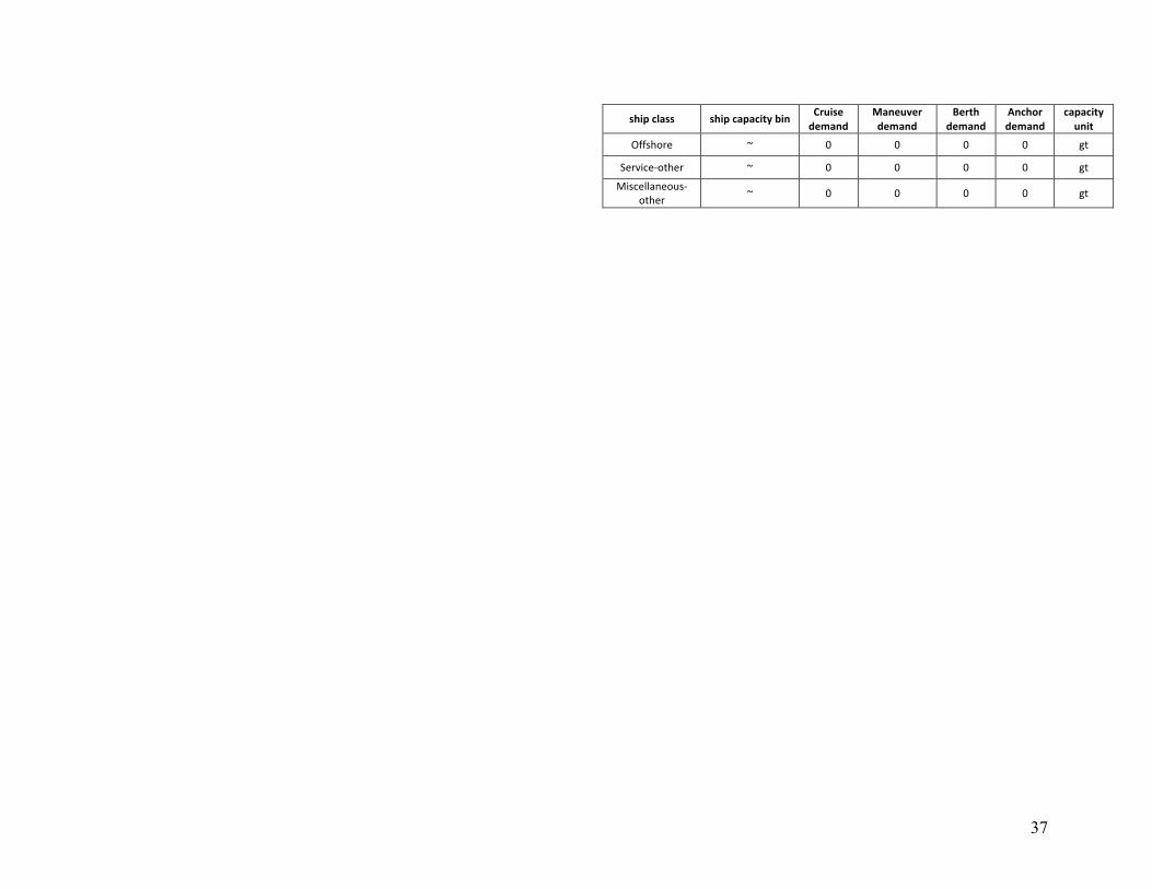
37

shipclass shipcapacitybin Cruisedemand

Maneuverdemand

Berthdemand

Anchordemand

capacityunit

Offshore ~ 0 0 0 0 gt

Service-other ~ 0 0 0 0 gt

Miscellaneous-

other~ 0 0 0 0 gt

38

Appendix E. Main engine emission factors for all pollutants except BC (g/kWh)

Pollutant Engine tier Engine type HFO (2.5% S) Distillate (0.14% S) 2015+ ECA fuel (0.1% S) LNG

CO2 All

SSD 607 593 593 -- MSD/HSD 670 658 658 --

GT/ST 950 962 962 -- LNG-Otto -- -- -- 457

LNG-diesel -- -- -- 366

NOx

Tier 0 0-130 rpm 18.10 17.01 17.01 -- >130 rpm 14.00 13.16 13.16 --

Tier I 0-130 rpm 17.00 15.98 15.98 --

130-1,999 rpm 0.94*45*rpm^(-0.2) 0.94*45*rpm^(-0.2) 0.94*45*rpm^(-0.2) -- 2,000+ rpm 9.80 9.21 9.21 --

Tier II 0-130 rpm 14.40 13.54 13.54 --

130-1,999 rpm 0.94*44*rpm^(-0.23) 0.94*44*rpm^(-0.23) 0.94*44*rpm^(-0.23) -- 2,000+ rpm 7.70 7.24 7.24 --

All

GT 6.10 5.92 5.92 -- ST 2.10 2.00 2.00 --

LNG-Otto -- -- -- 1.3 LNG-diesel -- -- -- 5

SOx

All

SSD 10.29 0.51 0.37 -- MSD/HSD 11.35 0.57 0.41 --

GT/ST 16.10 0.81 0.57 -- LNG-Otto -- -- -- 0.0027

LNG-diesel -- -- -- 0.0022

PM All

SSD 1.42 0.20 0.19 -- MSD/HSD 1.43 0.20 0.19 --

GT 0.06 0.01 0.01 -- ST 0.93 0.11 0.10 --

LNG-Otto -- -- -- 0.03 LNG-diesel -- -- -- 0.02

CO All

SSD/MSD/HSD 0.54 0.54 0.54 -- GT 0.10 0.10 0.10 -- ST 0.20 0.20 0.20 --

LNG-Otto -- -- -- 1.30 LNG-diesel -- -- -- 1.04

CH4 All

SSD/MSD/HSD 0.01 0.01 0.01 -- GT/ST 0.00 0.00 0.00 --

LNG-Otto -- -- -- 8.50 LNG-diesel -- -- -- 0.94

N2O All

SSD/MSD/HSD 0.03 0.03 0.03 --

GT/ST 0.05 0.04 0.04 -- LNG-Otto -- -- -- 0.02

LNG-diesel -- -- -- 0.01

39

Appendix F. Black carbon emission factors for main engines

The main engine BC emission factors used in this study are presented in Table F-3. These emission factors were used in a previous ICCT study, Comer et al. (in press), to develop a 2015 black carbon emissions inventory for global shipping. BC emission factors vary greatly in the literature. They are based on laboratory and onboard vessel tests measured from different sources using different methods. The BC emission factors used to compile global inventories are typically in the range of 0.18 to 1.08 g/kg fuel, with several prominent studies applying a 0.35 g BC/kg fuel emission factor for all fuel types and operating conditions. The evidence presented here suggests that a static BC emission factor fails to account for differences in engine stroke type, fuel type, and engine load. One recent comprehensive review of BC emission testing (University of California, Riverside [UCR], 2016) assessed the compiled evidence and concluded that “BC emission factors near the lower end of the 0.1 to 1.0 g/kg of fuel range found in the literature likely provide the best estimate for the more prevalent larger marine engines during at sea operation.” An approach to develop reasonable assumptions for emission factors as a function of engine stroke type, fuel type, and engine load is described herein. We based our BC emission factors on measurement data from UCR, Finland, and EUROMOT. UCR measured BC from two marine engines installed on two container ships. One engine was Tier II, the other was Tier 0 and was retrofitted with an exhaust gas cleaning system, or EGCS. Finland measured BC from one Tier 0 test marine engine in the laboratory. EUROMOT tested 35 marine engines in the lab. Five of those engines operated on residual fuels (i.e., HFO, RME, RMG), 20 operated on marine distillate fuels (i.e., MGO, DMA, DMB, DMX), six operated on ultralow-sulfur diesel (ULSD), and four operated on LNG. When developing marine BC emission factors, we focused on residual and marine distillate fuels and excluded ULSD and LNG to focus on the fuels most commonly used in international shipping. ULSD is used in some small ships, including some harbor craft, but is more expensive than marine distillate fuels such as MGO and is unlikely to be used in large oceangoing vessels. LNG is used in a very small fraction of the international fleet and LNG emits very low amounts of BC; thus, we decided to use the same LNG BC emission factor assumptions as Comer et al. (2017), as reported in Table F-3. Excluding the engines that operated on ULSD and LNG, we are left with 25 engines. BC from all but one of these engines was measured using the FSN method; the other was tested using the PAS method. We decided to exclude the BC emission factors from the engine tested using the PAS method in order maintain a consistent measurement method. Thus, we were left with 24 engines. Of these 24 engines, none were Tier 0, five were Tier I, 13 were Tier II, and six were Tier III. Altogether, we were left with results from 27 engines (24 EUROMOT + 2 UCR + 1 Finland), with 20 out of 27 (74%) Tier II or Tier III. The raw BC emission factors from the UCR, Finland, and EUROMOT tests are shown in Table F-2. The last column of Table F-2 reports emission factors in terms of g BC/kg fuel. UCR and Finland reported their BC emission factor results in both FSN units and in g/kg fuel. EUROMOT only reported in FSN units, requiring us to convert from FSN units to g/kg fuel. We did so as follows:

40

!"#$_&'(( = +" ∗ !"#$_-./

012,/ ∗ 4"56/ ∗ 78

where EFBC_mass = black carbon emission factor in mgBC/g fuel (equivalent to gBC/kg fuel) FSN = filter smoke number AF = air flow in kg/h EFBC_vol = black carbon emission factor in mgBC/m3 PME,l = main engine power at engine load l in kW SFOCl = specific fuel oil consumption at load l in g fuel/kWh DT = air density at exhaust temperature T in kg/m3 Specifically, the EFBC_vol is derived from on an equation from a presentation given by MAN,5 as follows:

!"#$_-./ =1

0.405∗ 5.23 ∗ "4@ ∗ A(C.DCEF∗GHI)

where EFBC_vol = black carbon emission factor in mgBC/m3 FSN = filter smoke number Note that the EFBC_vol assumes that the sample was taken using a heated sample line. There is a different EFBC_vol when using an unheated sample line.6 After the analysis, we discovered that one of the engines (29) used an unheated sample line. Applying the unheated EFBC_vol equation, we found that the difference between the BC EF estimates differed by only 1.7% to 6.1% when applying the heated line EFBC_vol equation. Because this small difference is unlikely to fundamentally change the results of the analysis, we decided to leave the BC EF uncorrected for engine 29 in the final report. And the SFOCl is based on Smith et al. (2015), as follows:

4"56/ = 4"56K'(L ∗ 0.405 ∗ MF − 0.71 ∗ M + 1.28 where SFOCl = specific fuel oil consumption at load l in g fuel/kWh

5 Lauer, P. (2016). Challenges of black carbon determination for marine diesel engines. Available at: http://www.theicct.org/sites/default/files/05-Challenges%20of%20Black%20Carbon%20Determination%20for%20Marine%20Diesel%20Engines%20-%20Peter%20Lauer%2C%20MAN%20Diesel%20and%20Turbo.pdf 6 EFBC_vol = (1/0.405)*4.95*FSN*e^(0.38*FSN)

41

SFOCbase = the baseline SFOC in g fuel/kWh, which is assumed to be 185 for SSD using distillate, 195 for SSD using residual, 205 for MSD using distillate, and 215 for MSD using residual

l = main engine load factor Lastly, the DT is calculated as follows:

78 =0

R ∗ S

where D = air density at exhaust temperature T in kg/m3 P = standard air pressure in kg/m/s2, equal to 101,325 Pa R = specific gas content for dry air, equal to 287.05 m2/s2/K

T = exhaust temperature in K Figure F-1 and Figure F-2 show the relationship between BC emission factor (g BC/kg fuel) and engine load (%) for 2-stroke engines operating on residual fuel or distillate fuel and for 4-stroke engines operating on residual fuel or distillate fuel, respectively. The open circles represent raw data from EUROMOT, UCR, and Finnish research. Table F-2 summarizes the data in these two figures, identifying the data source, engine type (including engine stroke type), fuel type, engine load, and measured BC emission factor. All BC emission factors in these figures and tables were measured using the FSN method with AVL 415S or AVL 415SE smoke meters.

42

Figure F-1. Raw black carbon emission factors for 2-stroke main engines using residual fuel (red) and distillate fuel (gray).

43

Figure F-2. Raw black carbon emission factors for 4-stroke main engines using residual fuel (red) and distillate fuel (gray).

The raw data suggest emission factors well below those recommended by UCR (2016) for use in global inventories. For example, as shown in Figure F-1, the best fit line to the raw data for 2-stroke engines using residual fuel indicates a BC emission factor of 0.09 g/kg fuel at 25% load and 0.06 g/kg fuel at 75% load. Emission factors for 2-stroke engines operating on distillate fuel are roughly 80% lower: 0.02 g/kg fuel at 25% load and 0.013 g/kg fuel at 75% load. Although we believe the general relationship of increasing BC emission factors with decreasing engine load is correct, the BC emission factors generated from these raw data may be biased low and therefore not representative of the global fleet, for the following reasons:

• Emissions from generally new, well-maintained engines were tested. Emissions from older in-service engines that may not be as well-maintained are expected to be higher.

• Laboratory testing was completed under steady-state conditions with constant, well-controlled engine speeds. In contrast, emissions may be higher for real marine engines under transient conditions with continually changing wind and wave conditions.

• Emissions from modern Tier II and Tier III engines do not likely represent emissions from ships in the global fleet. The raw BC emission factor curves represent emissions from six Tier III engines, 14 Tier II engines, five low-hour Tier I engines, and only two Tier 0 engines. Thus, 20 out of the 27 engines (74%) were modern Tier II or Tier III engines. Evidence presented in this report and by UCR (2016) suggests that modern, electronically controlled engines emit less BC than older engines. Given that 86% of the fleet has Tier 0 or Tier I engines (Table 1), emission factors measured from new, well-

44

maintained Tier II and Tier III engines are likely to be lower than those from engines in the global fleet.

• Variations in fuel quality can influence BC emission factors in the global fleet. In general, poorer quality fuels emit more BC than higher quality fuels. The test fuels available in Europe and North America may be of higher quality than fuels from other regions.

Reflecting these factors, the UCR (2016) report recommended BC emission factors toward the lower end of the 0.1 to 1.0 g/kg fuel range for global inventory development. We take this to mean that a representative BC emission factor for fuel consumed in diesel engine powered ships in the global fleet falls somewhere in this range. As shown in Figure F-1, 2-stroke engines operating on residual fuel accounted for the majority (71%) of fuel oil consumption in 2015. It is reasonable to limit BC emission factors to a minimum of 0.1 g/kg fuel for 2-stroke engines operating on residual fuel and to adjust the BC emission factors derived from the raw data for other engine stroke type and fuel type combinations accordingly. First, we took the best fit line for the raw BC emission factor for a 2-stroke engine operating on residual fuel, represented by the following equation: y = 0.0574*(x-0.359) Note that when x = 1, which is equivalent to 100% engine load, an emission factor of 0.0574 g BC per kg of fuel is estimated. To set the minimum BC emission factor for a 2-stroke engine operating on residual fuel to equal 0.1 g/kg fuel, the equation is modified as follows: y = 0.1*(x-0.359) Now, when x = 1, a ship using a 2-stroke engine operating on residual fuel is estimated to emit 0.1 g BC per kg fuel. The equation above defines the lower bound for BC emission factors for 2-stroke engines operating on residual fuel. This lower bound equation for the 2-stroke engine operating on residual fuel is subsequently used as a reference to set the BC emission factor curves for other engine stroke type/fuel type combinations, as described next. The equations describing the best fit to the raw data take the following form:

T = U ∗ VW where y = black carbon emission factor (g BC/kg fuel) U = coefficient; equivalent to the black carbon emission factor when engine load equals 100% x = engine load

45

b = exponent derived from the best fit power curve Original best fit equations were as follows: 2R0: y = 0.0574*(x-0.359) 2D0: y = 0.0119*(x-0.397) 4R0: y = 0.0953*(x-0.968) 4D0: y = 0.0460*(x-1.124) To maintain the relationship between the BC emission factors for 2R, 2D, 4R, and 4D, the coefficients (a) must be modified based on the new coefficient for 2R. See row 2 in Table F-1 for the new coefficients that correspond to a 2R coefficient of 0.1. The last row of Table F-1 describes the method for deriving the new coefficients based on the relationship between the original 2R, 2D, 4R, and 4D coefficients.

Table F-1. Black carbon emission factor coefficients for lower bound curves A B C D 2Ra 2D 4R 4D

1 Old coefficient 0.0574 0.0119 0.0953 0.0460

2 New coefficient 0.100 0.0207 0.1660 0.0801

Equation -- (B1/A1)*A2 (C1/A1)*A2 (D1/A1)*A2 a2R = 2-stroke engine operating on residual; 2D = 2-stroke engine operating on distillate; 4R = 4-stroke engine operating on

residual; 4D = 4-stroke engine operating on distillate

The new coefficients (Table F-1) are used to develop the lower bound emission factor equations for each engine stroke type/fuel type pair, denoted by subscript L as follows: 2RL: y = 0.1000*(x-0.359) 2DL: y = 0.0207*(x-0.397) 4RL: y = 0.1660*(x-0.968) 4DL: y = 0.0801*(x-1.124) Recognizing the uncertainty of developing BC emission factors, we developed an upper bound BC emission factor for each engine stroke type/fuel type pair. Buffaloe et al. (2014) found that on average BC emission factors doubled with one positive standard deviation from the mean across three plume intercept studies from ships at sea. The BC emission factors here are based on direct, in-stack measurements, but nearly all of the data were from laboratory tests under carefully controlled conditions, and could be biased low, as previously discussed. Thus, we believe doubling the lower bound estimates provides a reasonable range of uncertainty in actual

46

BC emissions from the in-use global fleet. Our best BC emission factor estimate is the midpoint between the lower and upper bounds at a given engine load. The lower, upper, and best estimate BC emission factor curves for 2-stroke engines operating on residual or distillate fuels are shown in Figure F-3. The same is shown for 4-stroke engines in Figure F-4.

Figure F-3. Black carbon emission factor curves for 2-stroke main engines.

Figure F-4. Black carbon emission factor curves for 4-stroke main engines.

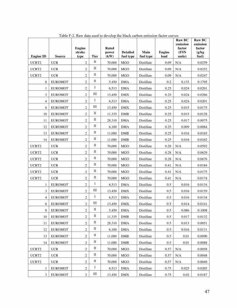
47

Table F-2. Raw data used to develop the black carbon emission factor curves

Engine ID Source

Engine stroke type Tier

Rated power (kW)

Detailed fuel type

Main fuel type

Engine load

Raw BC emission

factor (FSN units)

Raw BC emission

factor (g/kg fuel)

UCRT2 UCR 2 II 70,000 MGO Distillate 0.09 N/A 0.0259

UCRT2 UCR 2 II 70,000 MGO Distillate 0.09 N/A 0.0252

UCRT2 UCR 2 II 70,000 MGO Distillate 0.09 N/A 0.0247

8 EUROMOT 2 II 5,450 DMA Distillate 0.2 0.133 0.1795

1 EUROMOT 2 I 6,513 DMA Distillate 0.25 0.024 0.0201

3 EUROMOT 2 III 13,450 DMX Distillate 0.25 0.024 0.0266

4 EUROMOT 2 I 6,513 DMA Distillate 0.25 0.024 0.0201

6 EUROMOT 2 III 13,450 DMX Distillate 0.25 0.015 0.0175

10 EUROMOT 2 II 11,335 DMB Distillate 0.25 0.015 0.0128

11 EUROMOT 2 II 28,310 DMA Distillate 0.25 0.017 0.0075

12 EUROMOT 2 II 6,100 DMA Distillate 0.25 0.009 0.0084

13 EUROMOT 2 II 11,080 DMB Distillate 0.25 0.016 0.0165

14 EUROMOT 2 II 11,080 DMB Distillate 0.25 0.016 0.0162

UCRT2 UCR 2 II 70,000 MGO Distillate 0.28 N/A 0.0592

UCRT2 UCR 2 II 70,000 MGO Distillate 0.28 N/A 0.0629

UCRT2 UCR 2 II 70,000 MGO Distillate 0.28 N/A 0.0676

UCRT2 UCR 2 II 70,000 MGO Distillate 0.41 N/A 0.0184

UCRT2 UCR 2 II 70,000 MGO Distillate 0.41 N/A 0.0175

UCRT2 UCR 2 II 70,000 MGO Distillate 0.41 N/A 0.0174

1 EUROMOT 2 I 6,513 DMA Distillate 0.5 0.016 0.0134

3 EUROMOT 2 III 13,450 DMX Distillate 0.5 0.016 0.0159

4 EUROMOT 2 I 6,513 DMA Distillate 0.5 0.016 0.0134

6 EUROMOT 2 III 13,450 DMX Distillate 0.5 0.014 0.0141

8 EUROMOT 2 II 5,450 DMA Distillate 0.5 0.086 0.1008

10 EUROMOT 2 II 11,335 DMB Distillate 0.5 0.017 0.0132

11 EUROMOT 2 II 28,310 DMA Distillate 0.5 0.013 0.0051

12 EUROMOT 2 II 6,100 DMA Distillate 0.5 0.016 0.0131

13 EUROMOT 2 II 11,080 DMB Distillate 0.5 0.01 0.0090

14 EUROMOT 2 II 11,080 DMB Distillate 0.5 0.01 0.0088

UCRT2 UCR 2 II 70,000 MGO Distillate 0.57 N/A 0.0058

UCRT2 UCR 2 II 70,000 MGO Distillate 0.57 N/A 0.0048

UCRT2 UCR 2 II 70,000 MGO Distillate 0.57 N/A 0.0049

1 EUROMOT 2 I 6,513 DMA Distillate 0.75 0.025 0.0205

3 EUROMOT 2 III 13,450 DMX Distillate 0.75 0.02 0.0187

48

4 EUROMOT 2 I 6,513 DMA Distillate 0.75 0.025 0.0205

6 EUROMOT 2 III 13,450 DMX Distillate 0.75 0.015 0.0141

8 EUROMOT 2 II 5,450 DMA Distillate 0.75 0.036 0.0398

10 EUROMOT 2 II 11,335 DMB Distillate 0.75 0.02 0.0149

11 EUROMOT 2 II 28,310 DMA Distillate 0.75 0.013 0.0049

12 EUROMOT 2 II 6,100 DMA Distillate 0.75 0.025 0.0195

13 EUROMOT 2 II 11,080 DMB Distillate 0.75 0.013 0.0105

14 EUROMOT 2 II 11,080 DMB Distillate 0.75 0.012 0.0096

1 EUROMOT 2 I 6,513 DMA Distillate 0.85 0.015 0.0119

4 EUROMOT 2 I 6,513 DMA Distillate 0.85 0.015 0.0119

10 EUROMOT 2 II 11,335 DMB Distillate 0.85 0.023 0.0163

11 EUROMOT 2 II 28,310 DMA Distillate 0.85 0.011 0.0040

12 EUROMOT 2 II 6,100 DMA Distillate 0.85 0.016 0.0123

13 EUROMOT 2 II 11,080 DMB Distillate 0.85 0.012 0.0092

14 EUROMOT 2 II 11,080 DMB Distillate 0.85 0.014 0.0106

6 EUROMOT 2 III 13,450 DMX Distillate 0.9 0.011 0.0093

1 EUROMOT 2 I 6,513 DMA Distillate 1 0.018 0.0136

3 EUROMOT 2 III 13,450 DMX Distillate 1 0.016 0.0139

4 EUROMOT 2 I 6,513 DMA Distillate 1 0.018 0.0136

6 EUROMOT 2 III 13,450 DMX Distillate 1 0.014 0.0122

8 EUROMOT 2 II 5,450 DMA Distillate 1 0.03 0.0304

10 EUROMOT 2 II 11,335 DMB Distillate 1 0.025 0.0167

11 EUROMOT 2 II 28,310 DMA Distillate 1 0.018 0.0062

12 EUROMOT 2 II 6,100 DMA Distillate 1 0.032 0.0241

13 EUROMOT 2 II 11,080 DMB Distillate 1 0.022 0.0164

14 EUROMOT 2 II 11,080 DMB Distillate 1 0.028 0.0214

UCRT0pre UCR 2 0 16,600 HFO Residual 0.05 N/A 0.1690

15 EUROMOT 2 I 10,201 RMG Residual 0.1 0.179 0.1350

9 EUROMOT 2 I 6,509 RMG Residual 0.25 0.12 0.0977

15 EUROMOT 2 I 10,201 RMG Residual 0.25 0.132 0.1119

9 EUROMOT 2 I 6,509 RMG Residual 0.5 0.099 0.0780

15 EUROMOT 2 I 10,201 RMG Residual 0.5 0.087 0.0764

UCRT0pre UCR 2 0 16,600 HFO Residual 0.5 N/A 0.0420

9 EUROMOT 2 I 6,509 RMG Residual 0.75 0.112 0.0841

15 EUROMOT 2 I 10,201 RMG Residual 0.75 0.105 0.0882

UCRT0pre UCR 2 0 16,600 HFO Residual 0.75 N/A 0.0350

15 EUROMOT 2 I 10,201 RMG Residual 0.85 0.105 0.0848

UCRT0pre UCR 2 0 16,600 HFO Residual 0.87 N/A 0.0300

9 EUROMOT 2 I 6,509 RMG Residual 1 0.097 0.0710

49

15 EUROMOT 2 I 10,201 RMG Residual 1 0.106 0.0837

25 EUROMOT 4 III 3,960 DMA Distillate 0.1 0.76 1.4346

17 EUROMOT 4 II 10,800 DMA Distillate 0.25 0.07 0.0579

18 EUROMOT 4 II 10,800 DMA Distillate 0.25 0.1 0.0910

19 EUROMOT 4 II 10,350 DMA Distillate 0.25 0.15 0.1761

20 EUROMOT 4 II 5,000 DMA Distillate 0.25 0.13 0.1275

21 EUROMOT 4 II 6,000 DMA Distillate 0.25 0.12 0.1082

27 EUROMOT 4 III 8,000 DMA Distillate 0.25 0.216 0.2258

16 EUROMOT 4 III 7,200 DMA Distillate 0.5 0.11 0.1062

17 EUROMOT 4 II 10,800 DMA Distillate 0.5 0.05 0.0432

18 EUROMOT 4 II 10,800 DMA Distillate 0.5 0.16 0.1412

19 EUROMOT 4 II 10,350 DMA Distillate 0.5 0.07 0.0385

20 EUROMOT 4 II 5,000 DMA Distillate 0.5 0.12 0.1051

21 EUROMOT 4 II 6,000 DMA Distillate 0.5 0.13 0.1108

24 EUROMOT 4 III 3,960 DMA Distillate 0.5 0.404 0.4382

25 EUROMOT 4 III 3,960 DMA Distillate 0.5 0.226 0.2391

27 EUROMOT 4 III 8,000 DMA Distillate 0.5 0.175 0.1706

16 EUROMOT 4 III 7,200 DMA Distillate 0.75 0.07 0.0574

17 EUROMOT 4 II 10,800 DMA Distillate 0.75 0.06 0.0469

18 EUROMOT 4 II 10,800 DMA Distillate 0.75 0.18 0.1593

19 EUROMOT 4 II 10,350 DMA Distillate 0.75 0.05 0.0471

20 EUROMOT 4 II 5,000 DMA Distillate 0.75 0.07 0.0573

21 EUROMOT 4 II 6,000 DMA Distillate 0.75 0.14 0.1113

24 EUROMOT 4 III 3,960 DMA Distillate 0.75 0.264 0.2947

25 EUROMOT 4 III 3,960 DMA Distillate 0.75 0.1 0.0977

27 EUROMOT 4 III 8,000 DMA Distillate 0.75 0.079 0.0720

16 EUROMOT 4 III 7,200 DMA Distillate 0.85 0.05 0.0402

17 EUROMOT 4 II 10,800 DMA Distillate 0.85 0.04 0.0302

18 EUROMOT 4 II 10,800 DMA Distillate 0.85 0.05 0.0384

19 EUROMOT 4 II 10,350 DMA Distillate 0.85 0.03 0.0258

21 EUROMOT 4 II 6,000 DMA Distillate 0.85 0.06 0.0419

16 EUROMOT 4 III 7,200 DMA Distillate 1 0.05 0.0390

17 EUROMOT 4 II 10,800 DMA Distillate 1 0.05 0.0389

18 EUROMOT 4 II 10,800 DMA Distillate 1 0.08 0.0638

19 EUROMOT 4 II 10,350 DMA Distillate 1 0.03 0.0249

20 EUROMOT 4 II 5,000 DMA Distillate 1 0.04 0.0290

21 EUROMOT 4 II 6,000 DMA Distillate 1 0.06 0.0412

24 EUROMOT 4 III 3,960 DMA Distillate 1 0.135 0.1375

25 EUROMOT 4 III 3,960 DMA Distillate 1 0.048 0.0410

50

27 EUROMOT 4 III 8,000 DMA Distillate 1 0.056 0.0447

16 EUROMOT 4 III 7,200 DMA Distillate 1 0.07 0.0542

Finland_D Finland 4 0 1,640 MGO Distillate 0.25 N/A 0.4110

Finland_D Finland 4 0 1,640 MGO Distillate 0.25 N/A 0.3800

Finland_D Finland 4 0 1,640 MGO Distillate 0.75 N/A 0.0560

Finland_D Finland 4 0 1,640 MGO Distillate 0.75 N/A 0.0500

22 EUROMOT 4 II 3,498 HFO Residual 0.1 0.497 0.6887

23 EUROMOT 4 II 3,498 HFO Residual 0.1 0.499 0.7134

29 EUROMOT 4 I 3,480 RME Residual 0.1 1.2 1.8530

22 EUROMOT 4 II 3,498 HFO Residual 0.25 0.34 0.3107

23 EUROMOT 4 II 3,498 HFO Residual 0.25 0.32 0.2982

29 EUROMOT 4 I 3,480 RME Residual 0.25 0.35 0.3355

22 EUROMOT 4 II 3,498 HFO Residual 0.5 0.235 0.1961

23 EUROMOT 4 II 3,498 HFO Residual 0.5 0.254 0.2160

29 EUROMOT 4 I 3,480 RME Residual 0.5 0.13 0.1069

22 EUROMOT 4 II 3,498 HFO Residual 0.75 0.163 0.1252

23 EUROMOT 4 II 3,498 HFO Residual 0.75 0.163 0.1260

29 EUROMOT 4 I 3,480 RME Residual 0.75 0.14 0.1062

22 EUROMOT 4 II 3,498 HFO Residual 1 0.153 0.1076

23 EUROMOT 4 II 3,498 HFO Residual 1 0.146 0.1032

29 EUROMOT 4 I 3,480 RME Residual 1 0.15 0.1086

Finland_R Finland 4 0 1,640 HFO Residual 0.25 N/A 0.4300

Finland_R Finland 4 0 1,640 HFO Residual 0.75 N/A 0.1550

51

Table F-3. Black carbon main engine emission factors

Engine Load (%) Engine Type Unit

HFO Distillate LNG

2-stroke 4-stroke 2-stroke 4-stroke £ 5 SSD/MSD/HSD g/kg fuel 0.44

(0.29-0.59) 4.52

(3.02-6.03) 0.10

(0.07-0.14) 3.48

(2.32-4.65) --

10 SSD/MSD/HSD g/kg fuel 0.34 (0.23-0.46)

2.31 (1.54-3.08)

0.08 (0.05-0.10)

1.60 (1.07-2.13)

--

15 SSD/MSD/HSD g/kg fuel 0.30 (0.20-0.40)

1.56 (1.04-2.08)

0.07 (0.04-0.09)

1.01 (0.68-1.35)

--

20 SSD/MSD/HSD g/kg fuel 0.27 (0.18-0.36)

1.18 (0.79-1.58)

0.06 (0.04-0.08)

0.73 (0.49-0.98)

--

25 SSD/MSD/HSD g/kg fuel 0.25 (0.16-0.33)

0.95 (0.64-1.27)

0.05 (0.04-0.07)

0.57 (0.38-0.76)

--

30 SSD/MSD/HSD g/kg fuel 0.23 (0.15-0.31)

0.80 (0.53-1.06)

0.05 (0.03-0.07)

0.46 (0.31-0.62)

--

35 SSD/MSD/HSD g/kg fuel 0.22 (0.15-0.29)

0.69 (0.46-0.92)

0.05 (0.03-0.06)

0.39 (0.26-0.52)

--

40 SSD/MSD/HSD g/kg fuel 0.21 (0.14-0.28)

0.60 (0.40-0.81)

0.04 (0.03-0.06)

0.34 (0.22-0.45)

--

45 SSD/MSD/HSD g/kg fuel 0.20 (0.13-0.27)

0.54 (0.36-0.72)

0.04 (0.03-0.06)

0.29 (0.20-0.39)

--

50 SSD/MSD/HSD g/kg fuel 0.19 (0.13-0.26)

0.49 (0.32-0.65)

0.04 (0.03-0.05)

0.26 (0.17-0.35)

--

55 SSD/MSD/HSD g/kg fuel 0.19 (0.12-0.25)

0.44 (0.30-0.59)

0.04 (0.03-0.05)

0.24 (0.16-0.31)

--

60 SSD/MSD/HSD g/kg fuel 0.18 (0.12-0.24)

0.41 (0.27-0.54)

0.04 (0.03-0.05)

0.21 (0.14-0.28)

--

65 SSD/MSD/HSD g/kg fuel 0.18 (0.12-0.23)

0.38 (0.25-0.50)

0.04 (0.02-0.05)

0.19 (0.13-0.26)

--

70 SSD/MSD/HSD g/kg fuel 0.17 (0.11-0.23)

0.35 (0.23-0.47)

0.04 (0.02-0.05)

0.18 (0.12-0.24)

--

75 SSD/MSD/HSD g/kg fuel 0.17 (0.11-0.22)

0.33 (0.22-0.44)

0.03 (0.02-0.05)

0.17 (0.11-0.22)

--

80 SSD/MSD/HSD g/kg fuel 0.16 (0.11-0.22)

0.31 (0.21-0.41)

0.03 (0.02-0.05)

0.15 (0.10-0.21)

--

85 SSD/MSD/HSD g/kg fuel 0.16 (0.11-0.21)

0.29 (0.19-0.39)

0.03 (0.02-0.04)

0.14 (0.10-0.19)

--

90 SSD/MSD/HSD g/kg fuel 0.16 (0.11-0.21)

0.28 (0.18-0.37)

0.03 (0.02-0.04)

0.14 (0.09-0.18)

--

95 SSD/MSD/HSD g/kg fuel 0.15 (0.10-0.21)

0.26 (0.17-0.35)

0.03 (0.02-0.04)

0.13 (0.08-0.17)

--

100 SSD/MSD/HSD g/kg fuel 0.15 (0.10-0.21)

0.25 (0.17-0.35)

0.03 (0.02-0.04)

0.12 (0.08-0.17)

--

All ST g/kWh 0.08 0.08 0.06 0.06 -- All GT g/kWh 0.005 0.005 0.004 0.004 -- All LNG-Otto g/kWh -- -- -- -- 0.003 All LNG-Diesel g/kWh -- -- -- -- 0.002

52

Appendix G. Auxiliary engine emission factors (g/kWh)

Pollutant Engine tier Engine type HFO (2.5% S) Distillate (0.14% S) 2015+ ECA fuel (0.1% S) LNG

CO2 All

SSD/MSD/HSD 707 696 696 --

LNG-Otto -- -- -- 457

LNG-diesel -- -- -- 366

NOX

Tier 0 All rpms 14.70 13.82 13.82 --

Tier I

0-130 rpm 13.00 12.22 12.22 --

130-1,999 rpm 0.94*45*rpm^(-0.2) 0.94*45*rpm^(-0.2) 0.94*45*rpm^(-0.2) --

2,000+ rpm 13.00 12.22 12.22 --

LNG-Otto -- -- -- 1.3

LNG-Diesel -- -- -- --

Tier II

0-130 rpm 11.20 10.53 10.53 --

130-1,999 rpm 0.94*44*rpm^(-0.23) 0.94*44*rpm^(-0.23) 0.94*44*rpm^(-0.23) --

2000+ rpm 11.20 10.53 10.53 --

LNG-Otto -- -- -- 1.3

LNG-Diesel -- -- -- 5

SOX All

SSD/MSD/HSD 11.98 0.60 0.43 --

LNG-Otto -- -- -- 0.0027 LNG-Diesel -- -- -- 0.0022

PM All

SSD/MSD/HSD 1.44 0.20 0.19 --

LNG-Otto -- -- -- 0.03

LNG-Diesel -- -- -- 0.02

CO All

SSD/MSD/HSD 0.54 0.54 0.54 -- LNG-Otto -- -- -- 1.30

LNG-Diesel -- -- -- 1.04

CH4 All

SSD/MSD/HSD 0.01 0.01 0.01 --

LNG-Otto -- -- -- 8.50

LNG-Diesel -- -- -- 0.94

N2O All

SSD/MSD/HSD 0.04 0.03 0.03 --

LNG-Otto -- -- -- 0.02

LNG-Diesel -- -- -- 0.01

BC All

SSD/MSD/HSD 0.12 0.06 0.06 --

LNG-Otto -- -- -- 0.003

LNG-Diesel -- -- -- 0.002

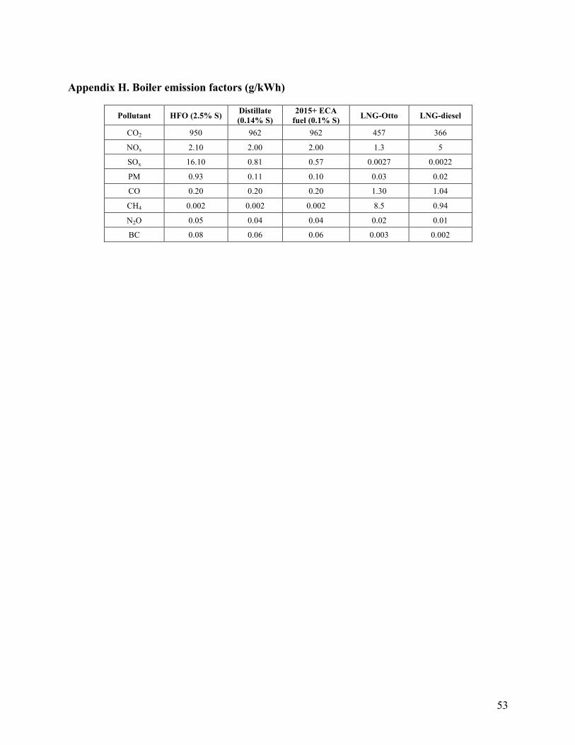
53

Appendix H. Boiler emission factors (g/kWh)

Pollutant HFO (2.5% S) Distillate (0.14% S)

2015+ ECA fuel (0.1% S) LNG-Otto LNG-diesel

CO2 950 962 962 457 366

NOx 2.10 2.00 2.00 1.3 5

SOx 16.10 0.81 0.57 0.0027 0.0022

PM 0.93 0.11 0.10 0.03 0.02

CO 0.20 0.20 0.20 1.30 1.04

CH4 0.002 0.002 0.002 8.5 0.94

N2O 0.05 0.04 0.04 0.02 0.01

BC 0.08 0.06 0.06 0.003 0.002

54

Appendix I. Low load adjustment factors for main engines

Load factor PM NOx SOx CO2 CO CH4 N2O ≤2% 7.29 4.63 1 1 9.7 21.18 4.63

3% 4.33 2.92 1 1 6.49 11.68 2.92 4% 3.09 2.21 1 1 4.86 7.71 2.21 5% 2.44 1.83 1 1 3.9 5.61 1.83 6% 2.04 1.6 1 1 3.26 4.35 1.6 7% 1.79 1.45 1 1 2.8 3.52 1.45 8% 1.61 1.35 1 1 2.45 2.95 1.35 9% 1.48 1.27 1 1 2.18 2.52 1.27

10% 1.38 1.22 1 1 1.97 2.18 1.22 11% 1.3 1.17 1 1 1.79 1.96 1.17 12% 1.24 1.14 1 1 1.64 1.76 1.14 13% 1.19 1.11 1 1 1.52 1.6 1.11 14% 1.15 1.08 1 1 1.41 1.47 1.08 15% 1.11 1.06 1 1 1.32 1.36 1.06 16% 1.08 1.05 1 1 1.24 1.26 1.05 17% 1.06 1.03 1 1 1.17 1.18 1.03 18% 1.04 1.02 1 1 1.11 1.11 1.02 19% 1.02 1.01 1 1 1.05 1.05 1.01 ≥20% 1 1 1 1 1 1 1

55

Appendix J: Average draught ratio by ship class

Ship Class 2013 2014 2015 Ballast Loaded Ballast Loaded Ballast Loaded

Ships with ballast-only voyages

Bulk carrier 0.58 0.92 0.58 0.91 0.57 0.91 Chemical tanker 0.66 0.88 0.66 0.88 0.65 0.89 General cargo 0.65 0.89 0.65 0.89 0.65 0.89 Liquefied gas tanker 0.67 0.89 0.67 0.89 0.67 0.88 Oil tanker 0.6 0.89 0.6 0.89 0.60 0.89 Other liquid tankers 0.67 0.90 0.69 0.91 0.67 0.90 Refrigerated bulk 0.69 0.88 0.69 0.88 0.68 0.88

Ships that typically do not have ballast-only voyages

Container 0.82 0.82 0.81 Cruise 0.98 0.98 0.97 Ferry pax only 0.90 0.90 0.90 Ferry ro-pax 0.93 0.93 0.92 Miscellaneous – fishing 0.85 0.84 0.84 Miscellaneous - others 0.54 0.50 0.47 Naval ship 0.84 0.83 0.82 Non-propelled 0.76 0.77 0.76 Non-Ship 0.71 0.93 0.95 Offshore 0.85 0.85 0.83 Ro-ro 0.87 0.87 0.87 Service other 0.86 0.86 0.86 Service tug 0.91 0.91 0.89 Vehicle 0.88 0.87 0.87 Yacht 0.93 0.93 0.92