GREEDY ALGORITHMS IN DATALOG

Sergio GrecoDip. Elettronica Informatica e Sistemistica

Universita della Calabria87030 Rende, Italygreco@si.deis.unical.it

Carlo ZanioloComputer Science Department

University of California at Los AngelesLos Angeles, CA 90024

zaniolo@cs.ucla.edu

Abstract

In the design of algorithms, the greedy paradigm provides a powerful toolfor solving efficiently classical computational problems, within the frame-work of procedural languages. However, expressing these algorithms withinthe declarative framework of logic-based languages has proven a difficult re-search challenge. In this paper, we extend the framework of Datalog-likelanguages to obtain simple declarative formulations for such problems, andpropose effective implementation techniques to ensure computational com-plexities comparable to those of procedural formulations. These advances areachieved through the use of the choice construct, extended with preferenceannotations to effect the selection of alternative stable-models and nonde-terministic fixpoints. We show that, with suitable storage structures, thedifferential fixpoint computation of our programs matches the complexity ofprocedural algorithms in classical search and optimization problems.

1

1 Introduction

The problem of finding efficient implementations for declarative logic-based lan-

guages represents one of the most arduous and lasting research challenges in com-

puter science. The interesting theoretical challenges posed by this problem are

made more urgent by the fact that extrema and other non-monotonic constructs

are needed to express many real-life applications, ranging from the ‘Bill of Materi-

als’ to graph-computation algorithms.

Significant progress in this area has been achieved on the semantic front, where

the introduction of the well-founded model semantics and stable-model semantics

allows us to assign a formal meaning to most, if not all, programs of practical

interest. Unfortunately, the computational problems remain largely unsolved: var-

ious approaches have been proposed to more effective computations of well-founded

models and stable models [26, 9], but these fall far short of matching the efficiency of

classical procedural solutions for say, algorithms that find shortest paths in graphs.

In general, it is known that determining whether a program has a stable model is

NP-complete [16].

Therefore, in this paper we propose a different approach: while, at the semantic

level, we strictly adhere to the formal declarative semantics of logic programs with

negation, we also allow the use of extended non-monotonic constructs with first

order semantics to facilitate the task of programmers and compilers alike. This en-

tails simple declarative formulations and nearly optimal executions for large classes

of problems that are normally solved using greedy algorithms.

Greedy algorithms [17] are those that solve a class of optimization problems,

using a control structure of a single loop, where, at each iteration some element

judged the ‘best’ at that stage is chosen and it is added to the solution. The simple

loop hints that these problems are amenable to a fixpoint computation. The choice

at each iteration calls attention to mechanisms by which nondeterministic choices

can be expressed in logic programs. This framework also provides an opportunity

of making, rather than blind choices, choices based on some heuristic criterion, such

as greedily choosing the least (or most) among the values at hand when seeking the

global minimization (or maximization) of the sum of such values. Following these

hints, this paper introduces primitives for choice and greedy selection, and shows

2

that classical greedy algorithms can be expressed using them. The paper also shows

how to translate each program with such constructs to a program which contains

only negation as nonmonotonic construct, and which defines the semantics of the

original program. Finally, several classes of programs with such constructs are de-

fined and it is shown that (i) they have stable model semantics (ii) they are easily

identifiable at compile time, and (iii) they can be optimized for efficient execution

—i.e., they yield the same complexities as those expected from greedy algorithms

in procedural programs. Thus, the approach provides a programmer with declara-

tive tools to express greedy algorithms, frees him/her from many implementation

details, yet guarantees good performance.

Previous work has shown that many nondeterministic decision problems can

be easily expressed in logic programs using the choice construct [22, 10]. In [11],

we showed that, while the semantic of choice requires the use of negation under

total stable model semantics, a stable model for these programs can be computed

in polynomial time. In fact, choice in Datalog programs stratified with respect to

negation achieves DB-PTIME completeness under genericity [1]. In this paper, we

further explore the ability of choice to express and support efficient computations,

by specializing choice with optimization heuristics expressed by the choice-least

and choice-most predicates. Then, we show that these two new built-in predicates

enable us to express easily greedy algorithms; furthermore, by using appropriate

data structures, the least-fixpoint computation of programs with choice-least and

choice-most emulate the classical greedy algorithms and matches their asymptotic

complexity.

A significant amount of excellent previous work has investigated the issue of how

to express in logic and compute efficiently greedy algorithms, and, more in general,

classical algorithms that require non-monotonic constructs. An incomplete list

include work by [23, 6, 21, 27, 7]. This line of research was often motivated by

the observation that many greedy algorithms can be viewed as optimized versions

of transitive closures. Efficient computation of transitive closures is central to

deductive database research, and the need for greedy algorithms is pervasive in

deductive database applications and in more traditional database applications such

as the Bill of Materials [29]. In this paper, we introduce a treatment for greedy

algorithms that is significant simpler and more robust than previous approaches

3

(including that of Greco, Zaniolo and Ganguly [13] where it was proposed to use

the choice together with the built-in predicates least and most); it also treats all

aspects of these algorithms, beginning from their intuitive formulation, and ending

with their optimized expression and execution.

The paper is organized as follows. In Section 2 we present basic definitions

on the syntax and semantics of Datalog. In Section 3, we introduce the notion of

choice and the stable-model declarative semantics of choice programs. In Section

4, we show how with this non-deterministic construct we can express in Datalog

algorithms such as single-source reachability and Hamiltonian path. A fixpoint-

based operational semantics for choice programs presented in Section 5, and this

semantics is then specialized with the introduction of the choice-least and choice-

most construct to force greedy selections among alternative choices. In Section

6, we show how the greedy refinement allow us to express greedy algorithms such

as Prim’s and Dijsktra’s. Finally, in Section 7, we turn to the implementation of

choice, choice-least and choice-most programs, and show that using well-known de-

ductive DB techniques, such as differential fixpoint, and suitable access structures,

such as hash tables and priority queues, we achieve optimal complexity bounds for

classical search problems.

2 Basic Notions

In this section, we summarize the basic notions of Horn Clauses logic, and its

extensions to allow negative goals.

A term is a variable, a constant, or a complex term of the form f(t1, . . . , tn),

where t1, . . . , tn are terms. An atom is a formula of the language that is of the

form p(t1, . . . , tn) where p is a predicate symbol of arity n. A literal is either an

atom (positive literal) or its negation (negative literal). A rule is a formula of the

language of the form

Q ← Q1, . . . , Qm.

where Q is a atom (head of the rule) and Q1, . . . , Qm are literals (body of the rule).

A term, atom, literal or rule is ground if it is variable free. A ground rule with

empty body is a fact. A logic program is a set of rules. A rule without negative

4

goals is called positive (a Horn clause); a program is called positive when all its

rules are positive. A DATALOG program is a positive program not containing

complex terms.

Let P be a program. Given two predicate symbols p and q in P , we say that

p directly depends on q, written p ≺ q if there exists a rule r in P such that p is

the head predicate symbol of r and q occurs in the body of r. The binary graph

representing this relation is called the dependency graph of P . The maximal strong

components of this graph will be called recursive cliques. Predicates in the same

recursive clique are mutually recursive. A rule is recursive if its head predicate

symbol is mutually recursive with some predicate symbol occurring in the body.

Given a logic program P , the Herbrand universe of P , denoted HP , is the set of

all possible ground terms recursively constructed by taking constants and function

symbols occurring in P . The Herbrand Base of P , denoted BP , is the set of all

possible ground atoms whose predicate symbols occur in P and whose arguments

are elements from the Herbrand universe. A ground instance of a rule r in P is a

rule obtained from r by replacing every variable X in r by a ground term in HP .

The set of ground instances of r is denoted by ground(r); accordingly, ground(P )

denotes⋃

r∈P ground(r). A (Herbrand) interpretation I of P is any subset of BP .

An model M of P is an interpretation that makes each ground instance of each rule

in P true (where a positive ground atom is true if and only if it belongs to M and a

negative ground atom is true if and only if it does not belong to M—total models).

A rule in ground(P ) whose body is true w.r.t. an interpretation I will also be called

fireable in I. Thus, a model for a program can be constructed by a procedure that

starts from I := ∅ and adds to I the head of a rule r ∈ ground(P ) that is firable in

I (this operation will be called firing r) until no firable rules remain. A model of

P is minimal if none of its proper subsets is a model. Each positive logic program

has a unique minimal model which defines its formal declarative semantics.

Given a program P and an interpretation M for P , we denote as groundM(P )

the program obtained from ground(P ) by

1. removing every rule having as a goals some literal ¬q with q ∈ M

2. removing all negated goals from the remaining rules.

5

Since groundM(P ) is a positive program, it has a unique minimal model. A

model M of P is said to be stable when M is also the minimum model of groundM(P )

[9]. A given program can have one or more stable (total) model, or possibly

none. Positive programs, stratified programs [4], locally stratified programs [19]

and weakly stratified programs [20] are among those that have exactly one stable

model.

Let I be an interpretation for a program P . The immediate consequence oper-

ator TP (I) is defined as the set containing the heads of each rule r ∈ ground(P )

s.t. all positive goals of r are in I, and none of the negated goals of r, is in I.

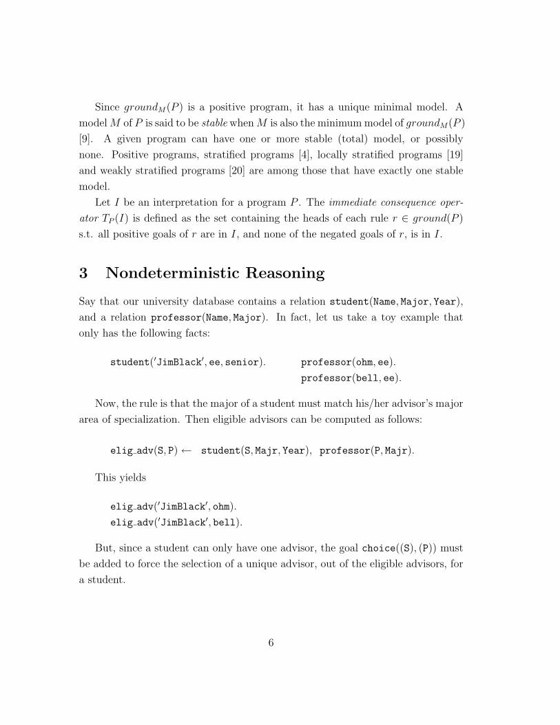
3 Nondeterministic Reasoning

Say that our university database contains a relation student(Name, Major, Year),

and a relation professor(Name, Major). In fact, let us take a toy example that

only has the following facts:

student(′JimBlack′, ee, senior). professor(ohm, ee).

professor(bell, ee).

Now, the rule is that the major of a student must match his/her advisor’s major

area of specialization. Then eligible advisors can be computed as follows:

elig adv(S, P) ← student(S, Majr, Year), professor(P, Majr).

This yields

elig adv(′JimBlack′, ohm).

elig adv(′JimBlack′, bell).

But, since a student can only have one advisor, the goal choice((S), (P)) must

be added to force the selection of a unique advisor, out of the eligible advisors, for

a student.

6

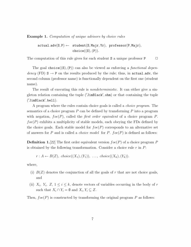
Example 1. Computation of unique advisors by choice rules

actual adv(S, P) ← student(S, Majr, Yr), professor(P, Majr),

choice((S), (P)).

The computation of this rule gives for each student S a unique professor P 2

The goal choice((S), (P)) can also be viewed as enforcing a functional depen-

dency (FD) S → P on the results produced by the rule; thus, in actual adv, the

second column (professor name) is functionally dependent on the first one (student

name).

The result of executing this rule is nondeterministic. It can either give a sin-

gleton relation containing the tuple (′JimBlack′, ohm) or that containing the tuple

(′JimBlack′, bell).

A program where the rules contain choice goals is called a choice program. The

semantics of a choice program P can be defined by transforming P into a program

with negation, foe(P ), called the first order equivalent of a choice program P .

foe(P ) exhibits a multiplicity of stable models, each obeying the FDs defined by

the choice goals. Each stable model for foe(P ) corresponds to an alternative set

of answers for P and is called a choice model for P . foe(P ) is defined as follows:

Definition 1.[22] The first order equivalent version foe(P ) of a choice program P

is obtained by the following transformation. Consider a choice rule r in P :

r : A ← B(Z), choice((X1), (Y1)), . . . , choice((Xk), (Yk)).

where,

(i) B(Z) denotes the conjunction of all the goals of r that are not choice goals,

and

(ii) Xi, Yi, Z, 1 ≤ i ≤ k, denote vectors of variables occurring in the body of r

such that Xi ∩ Yi = ∅ and Xi, Yi ⊆ Z.

Then, foe(P ) is constructed by transforming the original program P as follows:

7

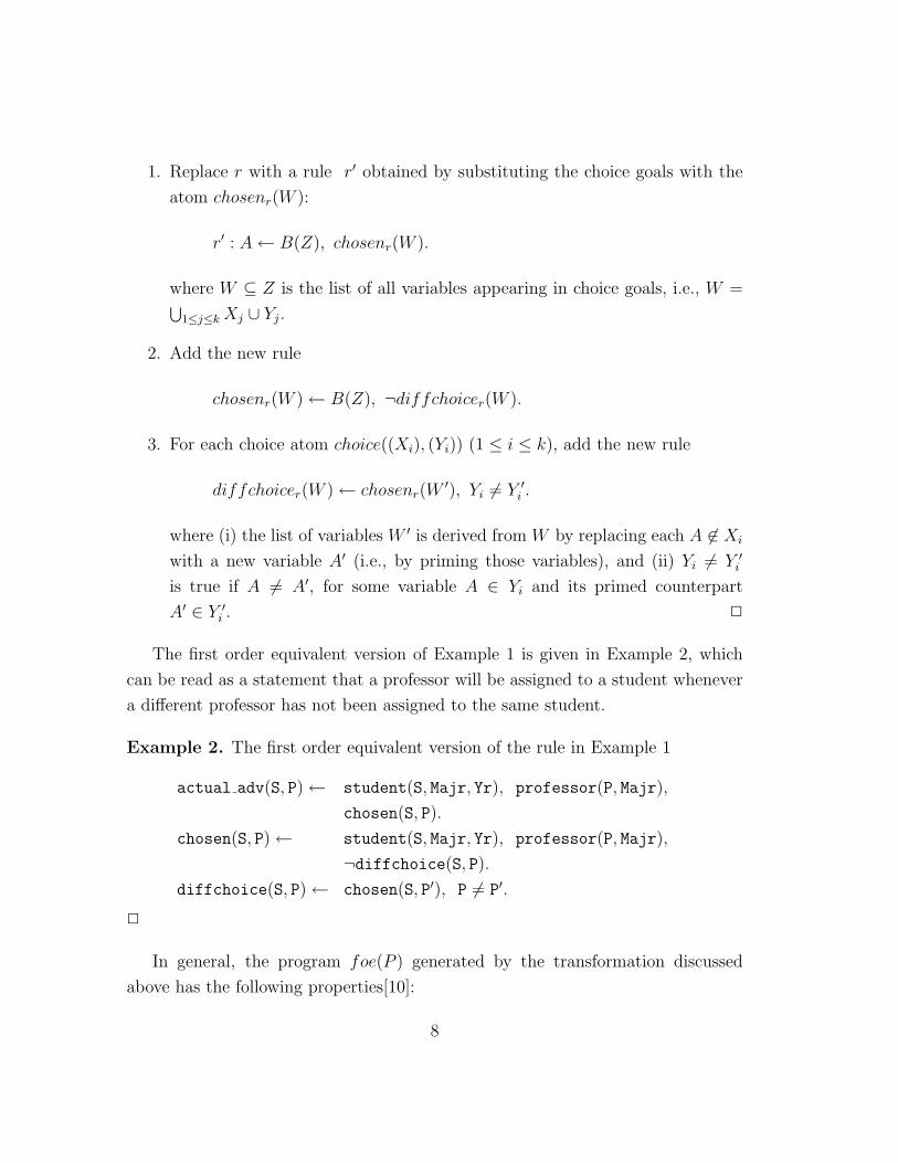
1. Replace r with a rule r′ obtained by substituting the choice goals with the

atom chosenr(W ):

r′ : A ← B(Z), chosenr(W ).

where W ⊆ Z is the list of all variables appearing in choice goals, i.e., W =⋃

1≤j≤k Xj ∪ Yj.

2. Add the new rule

chosenr(W ) ← B(Z), ¬diffchoicer(W ).

3. For each choice atom choice((Xi), (Yi)) (1 ≤ i ≤ k), add the new rule

diffchoicer(W ) ← chosenr(W′), Yi 6= Y ′

i .

where (i) the list of variables W ′ is derived from W by replacing each A 6∈ Xi

with a new variable A′ (i.e., by priming those variables), and (ii) Yi 6= Y ′i

is true if A 6= A′, for some variable A ∈ Yi and its primed counterpart

A′ ∈ Y ′i . 2

The first order equivalent version of Example 1 is given in Example 2, which

can be read as a statement that a professor will be assigned to a student whenever

a different professor has not been assigned to the same student.

Example 2. The first order equivalent version of the rule in Example 1

actual adv(S, P) ← student(S, Majr, Yr), professor(P, Majr),

chosen(S, P).

chosen(S, P) ← student(S, Majr, Yr), professor(P, Majr),

¬diffchoice(S, P).diffchoice(S, P) ← chosen(S, P′), P 6= P′.

2

In general, the program foe(P ) generated by the transformation discussed

above has the following properties[10]:

8

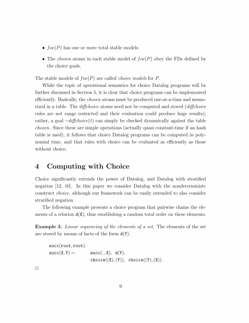
• foe(P ) has one or more total stable models.

• The chosen atoms in each stable model of foe(P ) obey the FDs defined by

the choice goals.

The stable models of foe(P ) are called choice models for P .

While the topic of operational semantics for choice Datalog programs will be

further discussed in Section 5, it is clear that choice programs can be implemented

efficiently. Basically, the chosen atoms must be produced one-at-a-time and memo-

rized in a table. The diffchoice atoms need not be computed and stored (diffchoice

rules are not range restricted and their evaluation could produce huge results);

rather, a goal ¬diffchoice(t) can simply be checked dynamically against the table

chosen. Since these are simple operations (actually quasi constant-time if an hash

table is used), it follows that choice Datalog programs can be computed in poly-

nomial time, and that rules with choice can be evaluated as efficiently as those

without choice.

4 Computing with Choice

Choice significantly extends the power of Datalog, and Datalog with stratified

negation [12, 10]. In this paper we consider Datalog with the nondeterministc

construct choice, although our framework can be easily extended to also consider

stratified negation.

The following example presents a choice program that pairwise chains the ele-

ments of a relation d(X), thus establishing a random total order on these elements.

Example 3. Linear sequencing of the elements of a set. The elements of the set

are stored by means of facts of the form d(Y).

succ(root, root).

succ(X, Y) ← succ( , X), d(Y),

choice((X), (Y)), choice((Y), (X)).

2

9

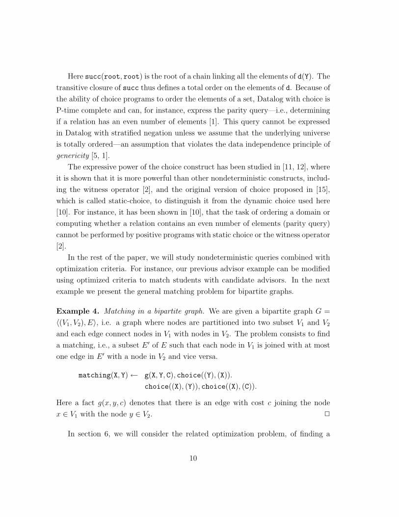
Here succ(root, root) is the root of a chain linking all the elements of d(Y). The

transitive closure of succ thus defines a total order on the elements of d. Because of

the ability of choice programs to order the elements of a set, Datalog with choice is

P-time complete and can, for instance, express the parity query—i.e., determining

if a relation has an even number of elements [1]. This query cannot be expressed

in Datalog with stratified negation unless we assume that the underlying universe

is totally ordered—an assumption that violates the data independence principle of

genericity [5, 1].

The expressive power of the choice construct has been studied in [11, 12], where

it is shown that it is more powerful than other nondeterministic constructs, includ-

ing the witness operator [2], and the original version of choice proposed in [15],

which is called static-choice, to distinguish it from the dynamic choice used here

[10]. For instance, it has been shown in [10], that the task of ordering a domain or

computing whether a relation contains an even number of elements (parity query)

cannot be performed by positive programs with static choice or the witness operator

[2].

In the rest of the paper, we will study nondeterministic queries combined with

optimization criteria. For instance, our previous advisor example can be modified

using optimized criteria to match students with candidate advisors. In the next

example we present the general matching problem for bipartite graphs.

Example 4. Matching in a bipartite graph. We are given a bipartite graph G =

〈(V1, V2), E〉, i.e. a graph where nodes are partitioned into two subset V1 and V2

and each edge connect nodes in V1 with nodes in V2. The problem consists to find

a matching, i.e., a subset E ′ of E such that each node in V1 is joined with at most

one edge in E ′ with a node in V2 and vice versa.

matching(X, Y) ← g(X, Y, C), choice((Y), (X)).

choice((X), (Y)), choice((X), (C)).

Here a fact g(x, y, c) denotes that there is an edge with cost c joining the node

x ∈ V1 with the node y ∈ V2. 2

In section 6, we will consider the related optimization problem, of finding a

10

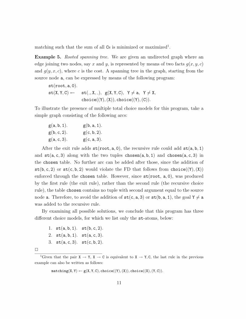
matching such that the sum of all Cs is minimized or maximized1.

Example 5. Rooted spanning tree. We are given an undirected graph where an

edge joining two nodes, say x and y, is represented by means of two facts g(x, y, c)

and g(y, x, c), where c is the cost. A spanning tree in the graph, starting from the

source node a, can be expressed by means of the following program:

st(root, a, 0).

st(X, Y, C) ← st( , X, ), g(X, Y, C), Y 6= a, Y 6= X,

choice((Y), (X)), choice((Y), (C)).

To illustrate the presence of multiple total choice models for this program, take a

simple graph consisting of the following arcs:

g(a, b, 1). g(b, a, 1).

g(b, c, 2). g(c, b, 2).

g(a, c, 3). g(c, a, 3).

After the exit rule adds st(root, a, 0), the recursive rule could add st(a, b, 1)

and st(a, c, 3) along with the two tuples chosen(a, b, 1) and chosen(a, c, 3) in

the chosen table. No further arc can be added after those, since the addition of

st(b, c, 2) or st(c, b, 2) would violate the FD that follows from choice((Y), (X))

enforced through the chosen table. However, since st(root, a, 0), was produced

by the first rule (the exit rule), rather than the second rule (the recursive choice

rule), the table chosen contains no tuple with second argument equal to the source

node a. Therefore, to avoid the addition of st(c, a, 3) or st(b, a, 1), the goal Y 6= a

was added to the recursive rule.

By examining all possible solutions, we conclude that this program has three

different choice models, for which we list only the st-atoms, below:

1. st(a, b, 1). st(b, c, 2).

2. st(a, b, 1). st(a, c, 3).

3. st(a, c, 3). st(c, b, 2).

2

1Given that the pair X → Y, X → C is equivalent to X → Y, C, the last rule in the previousexample can also be written as follows:

matching(X, Y) ← g(X, Y, C), choice((Y), (X)), choice((X), (Y, C)).

11

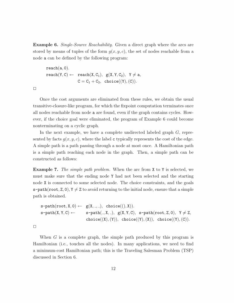
Example 6. Single-Source Reachability. Given a direct graph where the arcs are

stored by means of tuples of the form g(x, y, c), the set of nodes reachable from a

node a can be defined by the following program:

reach(a, 0).

reach(Y, C) ← reach(X, C1), g(X, Y, C2), Y 6= a,

C = C1 + C2, choice((Y), (C)).

2

Once the cost arguments are eliminated from these rules, we obtain the usual

transitive-closure-like program, for which the fixpoint computation terminates once

all nodes reachable from node a are found, even if the graph contains cycles. How-

ever, if the choice goal were eliminated, the program of Example 6 could become

nonterminating on a cyclic graph.

In the next example, we have a complete undirected labeled graph G, repre-

sented by facts g(x, y, c), where the label c typically represents the cost of the edge.

A simple path is a path passing through a node at most once. A Hamiltonian path

is a simple path reaching each node in the graph. Then, a simple path can be

constructed as follows:

Example 7. The simple path problem. When the arc from X to Y is selected, we

must make sure that the ending node Y had not been selected and the starting

node X is connected to some selected node. The choice constraints, and the goals

s-path(root, Z, 0), Y 6= Z to avoid returning to the initial node, ensure that a simple

path is obtained.

s-path(root, X, 0) ← g(X, , ), choice((), X)).

s-path(X, Y, C) ← s-path( , X, ), g(X, Y, C), s-path(root, Z, 0), Y 6= Z,

choice((X), (Y)), choice((Y), (X)), choice((Y), (C)).

2

When G is a complete graph, the simple path produced by this program is

Hamiltonian (i.e., touches all the nodes). In many applications, we need to find

a minimum-cost Hamiltonian path; this is the Traveling Salesman Problem (TSP)

discussed in Section 6.

12

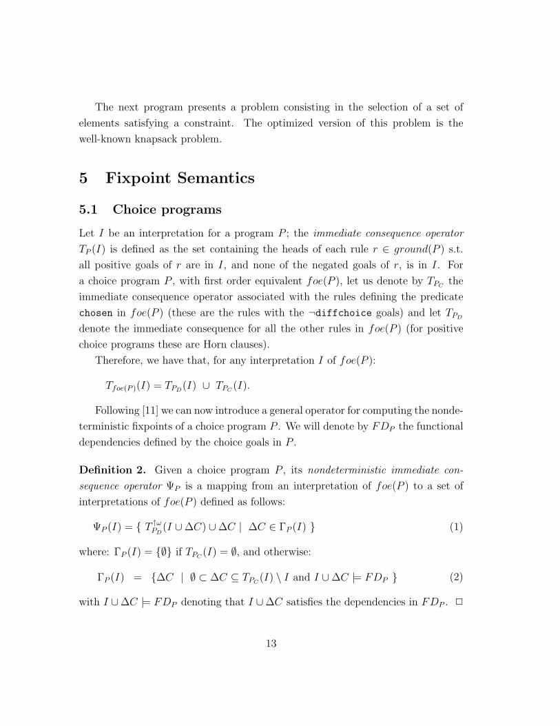
The next program presents a problem consisting in the selection of a set of

elements satisfying a constraint. The optimized version of this problem is the

well-known knapsack problem.

5 Fixpoint Semantics

5.1 Choice programs

Let I be an interpretation for a program P ; the immediate consequence operator

TP (I) is defined as the set containing the heads of each rule r ∈ ground(P ) s.t.

all positive goals of r are in I, and none of the negated goals of r, is in I. For

a choice program P , with first order equivalent foe(P ), let us denote by TPCthe

immediate consequence operator associated with the rules defining the predicate

chosen in foe(P ) (these are the rules with the ¬diffchoice goals) and let TPD

denote the immediate consequence for all the other rules in foe(P ) (for positive

choice programs these are Horn clauses).

Therefore, we have that, for any interpretation I of foe(P ):

Tfoe(P )(I) = TPD(I) ∪ TPC

(I).

Following [11] we can now introduce a general operator for computing the nonde-

terministic fixpoints of a choice program P . We will denote by FDP the functional

dependencies defined by the choice goals in P .

Definition 2. Given a choice program P , its nondeterministic immediate con-

sequence operator ΨP is a mapping from an interpretation of foe(P ) to a set of

interpretations of foe(P ) defined as follows:

ΨP (I) = { T ↑ωPD

(I ∪∆C) ∪∆C | ∆C ∈ ΓP (I) } (1)

where: ΓP (I) = {∅} if TPC(I) = ∅, and otherwise:

ΓP (I) = {∆C | ∅ ⊂ ∆C ⊆ TPC(I) \ I and I ∪∆C |= FDP } (2)

with I ∪∆C |= FDP denoting that I ∪∆C satisfies the dependencies in FDP . 2

13

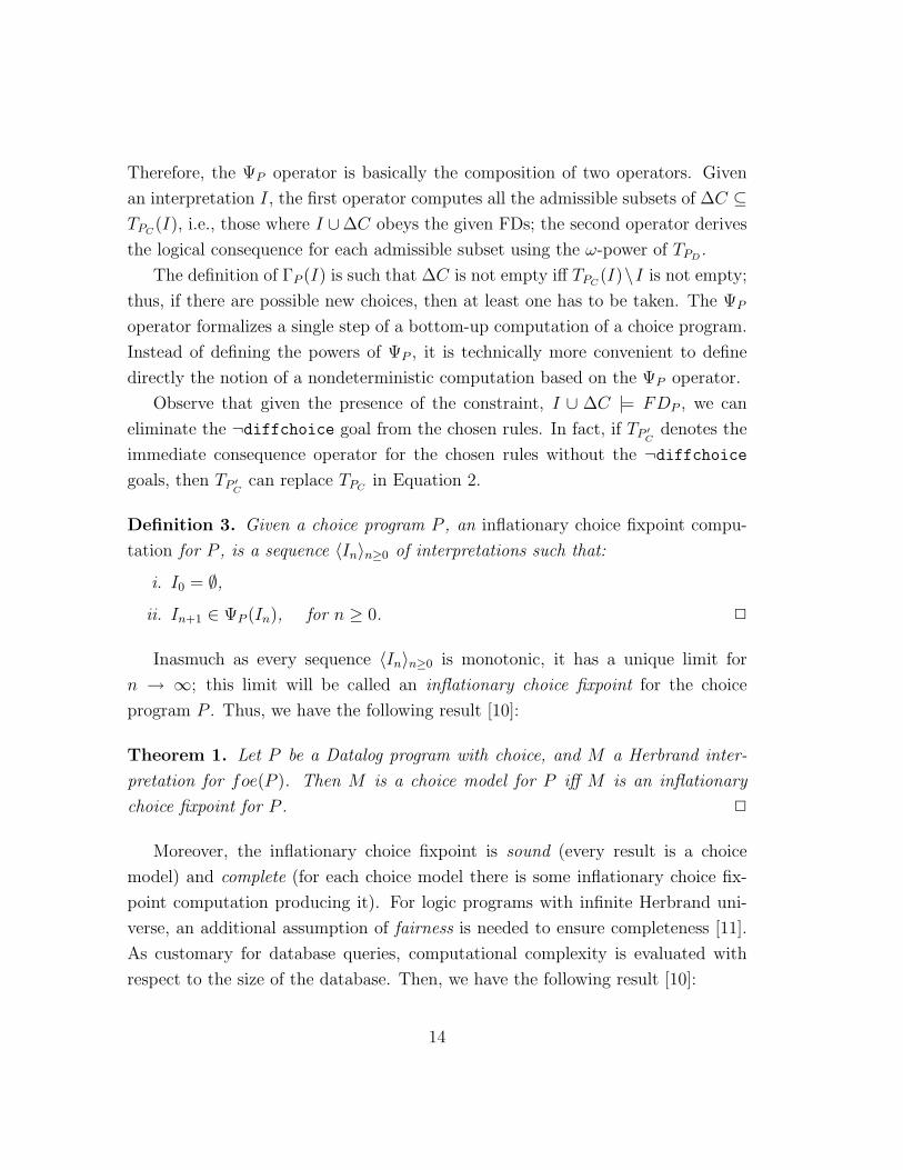
Therefore, the ΨP operator is basically the composition of two operators. Given

an interpretation I, the first operator computes all the admissible subsets of ∆C ⊆TPC

(I), i.e., those where I ∪∆C obeys the given FDs; the second operator derives

the logical consequence for each admissible subset using the ω-power of TPD.

The definition of ΓP (I) is such that ∆C is not empty iff TPC(I)\I is not empty;

thus, if there are possible new choices, then at least one has to be taken. The ΨP

operator formalizes a single step of a bottom-up computation of a choice program.

Instead of defining the powers of ΨP , it is technically more convenient to define

directly the notion of a nondeterministic computation based on the ΨP operator.

Observe that given the presence of the constraint, I ∪ ∆C |= FDP , we can

eliminate the ¬diffchoice goal from the chosen rules. In fact, if TP ′C denotes the

immediate consequence operator for the chosen rules without the ¬diffchoicegoals, then TP ′C can replace TPC

in Equation 2.

Definition 3. Given a choice program P , an inflationary choice fixpoint compu-

tation for P , is a sequence 〈In〉n≥0 of interpretations such that:

i. I0 = ∅,ii. In+1 ∈ ΨP (In), for n ≥ 0. 2

Inasmuch as every sequence 〈In〉n≥0 is monotonic, it has a unique limit for

n → ∞; this limit will be called an inflationary choice fixpoint for the choice

program P . Thus, we have the following result [10]:

Theorem 1. Let P be a Datalog program with choice, and M a Herbrand inter-

pretation for foe(P ). Then M is a choice model for P iff M is an inflationary

choice fixpoint for P . 2

Moreover, the inflationary choice fixpoint is sound (every result is a choice

model) and complete (for each choice model there is some inflationary choice fix-

point computation producing it). For logic programs with infinite Herbrand uni-

verse, an additional assumption of fairness is needed to ensure completeness [11].

As customary for database queries, computational complexity is evaluated with

respect to the size of the database. Then, we have the following result [10]:

14

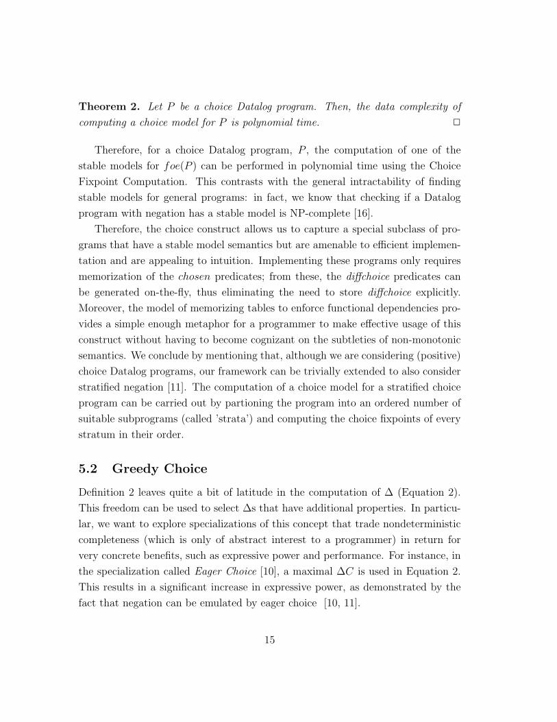
Theorem 2. Let P be a choice Datalog program. Then, the data complexity of

computing a choice model for P is polynomial time. 2

Therefore, for a choice Datalog program, P , the computation of one of the

stable models for foe(P ) can be performed in polynomial time using the Choice

Fixpoint Computation. This contrasts with the general intractability of finding

stable models for general programs: in fact, we know that checking if a Datalog

program with negation has a stable model is NP-complete [16].

Therefore, the choice construct allows us to capture a special subclass of pro-

grams that have a stable model semantics but are amenable to efficient implemen-

tation and are appealing to intuition. Implementing these programs only requires

memorization of the chosen predicates; from these, the diffchoice predicates can

be generated on-the-fly, thus eliminating the need to store diffchoice explicitly.

Moreover, the model of memorizing tables to enforce functional dependencies pro-

vides a simple enough metaphor for a programmer to make effective usage of this

construct without having to become cognizant on the subtleties of non-monotonic

semantics. We conclude by mentioning that, although we are considering (positive)

choice Datalog programs, our framework can be trivially extended to also consider

stratified negation [11]. The computation of a choice model for a stratified choice

program can be carried out by partioning the program into an ordered number of

suitable subprograms (called ’strata’) and computing the choice fixpoints of every

stratum in their order.

5.2 Greedy Choice

Definition 2 leaves quite a bit of latitude in the computation of ∆ (Equation 2).

This freedom can be used to select ∆s that have additional properties. In particu-

lar, we want to explore specializations of this concept that trade nondeterministic

completeness (which is only of abstract interest to a programmer) in return for

very concrete benefits, such as expressive power and performance. For instance, in

the specialization called Eager Choice [10], a maximal ∆C is used in Equation 2.

This results in a significant increase in expressive power, as demonstrated by the

fact that negation can be emulated by eager choice [10, 11].

15

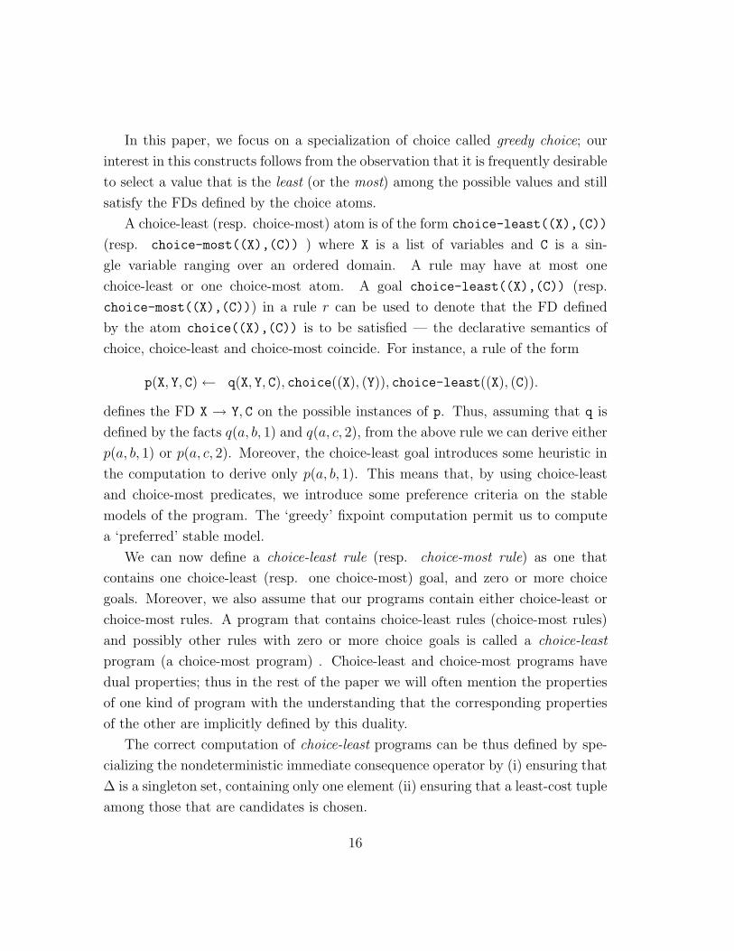
In this paper, we focus on a specialization of choice called greedy choice; our

interest in this constructs follows from the observation that it is frequently desirable

to select a value that is the least (or the most) among the possible values and still

satisfy the FDs defined by the choice atoms.

A choice-least (resp. choice-most) atom is of the form choice-least((X),(C))

(resp. choice-most((X),(C)) ) where X is a list of variables and C is a sin-

gle variable ranging over an ordered domain. A rule may have at most one

choice-least or one choice-most atom. A goal choice-least((X),(C)) (resp.

choice-most((X),(C))) in a rule r can be used to denote that the FD defined

by the atom choice((X),(C)) is to be satisfied — the declarative semantics of

choice, choice-least and choice-most coincide. For instance, a rule of the form

p(X, Y, C) ← q(X, Y, C), choice((X), (Y)), choice-least((X), (C)).

defines the FD X → Y, C on the possible instances of p. Thus, assuming that q is

defined by the facts q(a, b, 1) and q(a, c, 2), from the above rule we can derive either

p(a, b, 1) or p(a, c, 2). Moreover, the choice-least goal introduces some heuristic in

the computation to derive only p(a, b, 1). This means that, by using choice-least

and choice-most predicates, we introduce some preference criteria on the stable

models of the program. The ‘greedy’ fixpoint computation permit us to compute

a ‘preferred’ stable model.

We can now define a choice-least rule (resp. choice-most rule) as one that

contains one choice-least (resp. one choice-most) goal, and zero or more choice

goals. Moreover, we also assume that our programs contain either choice-least or

choice-most rules. A program that contains choice-least rules (choice-most rules)

and possibly other rules with zero or more choice goals is called a choice-least

program (a choice-most program) . Choice-least and choice-most programs have

dual properties; thus in the rest of the paper we will often mention the properties

of one kind of program with the understanding that the corresponding properties

of the other are implicitly defined by this duality.

The correct computation of choice-least programs can be thus defined by spe-

cializing the nondeterministic immediate consequence operator by (i) ensuring that

∆ is a singleton set, containing only one element (ii) ensuring that a least-cost tuple

among those that are candidates is chosen.

16

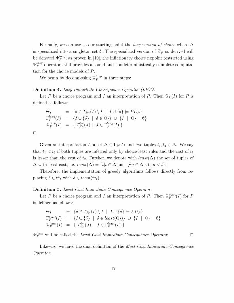
Formally, we can use as our starting point the lazy version of choice where ∆

is specialized into a singleton set δ. The specialized version of ΨP so derived will

be denoted ΨlazyP ; as proven in [10], the inflationary choice fixpoint restricted using

ΨlazyP operators still provides a sound and nondeterministically complete computa-

tion for the choice models of P .

We begin by decomposing ΨlazyP in three steps:

Definition 4. Lazy Immediate-Consequence Operator (LICO).

Let P be a choice program and I an interpretation of P . Then ΨP (I) for P is

defined as follows:

ΘI = {δ ∈ TPC(I) \ I | I ∪ {δ} |= FDP}

ΓlazyP (I) = {I ∪ {δ} | δ ∈ ΘI} ∪ {I | ΘI = ∅}

ΨlazyP (I) = { T ↑ω

PD(J) | J ∈ Γlazy

P (I) }2

Given an interpretation I, a set ∆ ∈ ΓP (I) and two tuples t1, t2 ∈ ∆. We say

that t1 < t2 if both tuples are inferred only by choice-least rules and the cost of t1

is lesser than the cost of t2. Further, we denote with least(∆) the set of tuples of

∆ with least cost, i.e. least(∆) = {t|t ∈ ∆ and 6 ∃u ∈ ∆ s.t. u < t}.Therefore, the implementation of greedy algorithms follows directly from re-

placing δ ∈ ΘI with δ ∈ least(ΘI).

Definition 5. Least-Cost Immediate-Consequence Operator.

Let P be a choice program and I an interpretation of P . Then ΨleastP (I) for P

is defined as follows:

ΘI = {δ ∈ TPC(I) \ I | I ∪ {δ} |= FDP}

ΓleastP (I) = {I ∪ {δ} | δ ∈ least(ΘI)} ∪ {I | ΘI = ∅}

ΨleastP (I) = { T ↑ω

PD(J) | J ∈ Γleast

P (I) }

ΨleastP will be called the Least-Cost Immediate-Consequence Operator. 2

Likewise, we have the dual definition of the Most-Cost Immediate-Consequence

Operator.

17

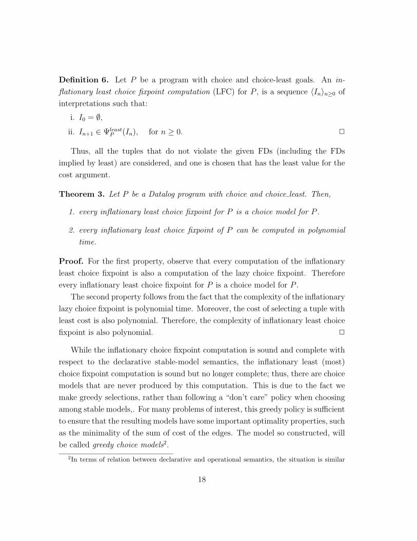
Definition 6. Let P be a program with choice and choice-least goals. An in-

flationary least choice fixpoint computation (LFC) for P , is a sequence 〈In〉n≥0 of

interpretations such that:

i. I0 = ∅,ii. In+1 ∈ Ψleast

P (In), for n ≥ 0. 2

Thus, all the tuples that do not violate the given FDs (including the FDs

implied by least) are considered, and one is chosen that has the least value for the

cost argument.

Theorem 3. Let P be a Datalog program with choice and choice least. Then,

1. every inflationary least choice fixpoint for P is a choice model for P .

2. every inflationary least choice fixpoint of P can be computed in polynomial

time.

Proof. For the first property, observe that every computation of the inflationary

least choice fixpoint is also a computation of the lazy choice fixpoint. Therefore

every inflationary least choice fixpoint for P is a choice model for P .

The second property follows from the fact that the complexity of the inflationary

lazy choice fixpoint is polynomial time. Moreover, the cost of selecting a tuple with

least cost is also polynomial. Therefore, the complexity of inflationary least choice

fixpoint is also polynomial. 2

While the inflationary choice fixpoint computation is sound and complete with

respect to the declarative stable-model semantics, the inflationary least (most)

choice fixpoint computation is sound but no longer complete; thus, there are choice

models that are never produced by this computation. This is due to the fact we

make greedy selections, rather than following a “don’t care” policy when choosing

among stable models,. For many problems of interest, this greedy policy is sufficient

to ensure that the resulting models have some important optimality properties, such

as the minimality of the sum of cost of the edges. The model so constructed, will

be called greedy choice models2.

2In terms of relation between declarative and operational semantics, the situation is similar

18

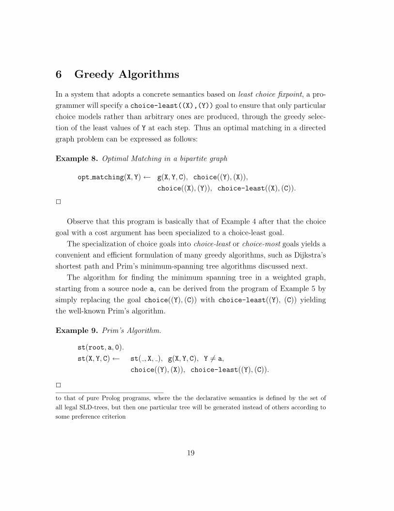
6 Greedy Algorithms

In a system that adopts a concrete semantics based on least choice fixpoint, a pro-

grammer will specify a choice-least((X),(Y)) goal to ensure that only particular

choice models rather than arbitrary ones are produced, through the greedy selec-

tion of the least values of Y at each step. Thus an optimal matching in a directed

graph problem can be expressed as follows:

Example 8. Optimal Matching in a bipartite graph

opt matching(X, Y) ← g(X, Y, C), choice((Y), (X)),

choice((X), (Y)), choice-least((X), (C)).

2

Observe that this program is basically that of Example 4 after that the choice

goal with a cost argument has been specialized to a choice-least goal.

The specialization of choice goals into choice-least or choice-most goals yields a

convenient and efficient formulation of many greedy algorithms, such as Dijkstra’s

shortest path and Prim’s minimum-spanning tree algorithms discussed next.

The algorithm for finding the minimum spanning tree in a weighted graph,

starting from a source node a, can be derived from the program of Example 5 by

simply replacing the goal choice((Y), (C)) with choice-least((Y), (C)) yielding

the well-known Prim’s algorithm.

Example 9. Prim’s Algorithm.

st(root, a, 0).

st(X, Y, C) ← st( , X, ), g(X, Y, C), Y 6= a,

choice((Y), (X)), choice-least((Y), (C)).

2

to that of pure Prolog programs, where the the declarative semantics is defined by the set ofall legal SLD-trees, but then one particular tree will be generated instead of others according tosome preference criterion

19

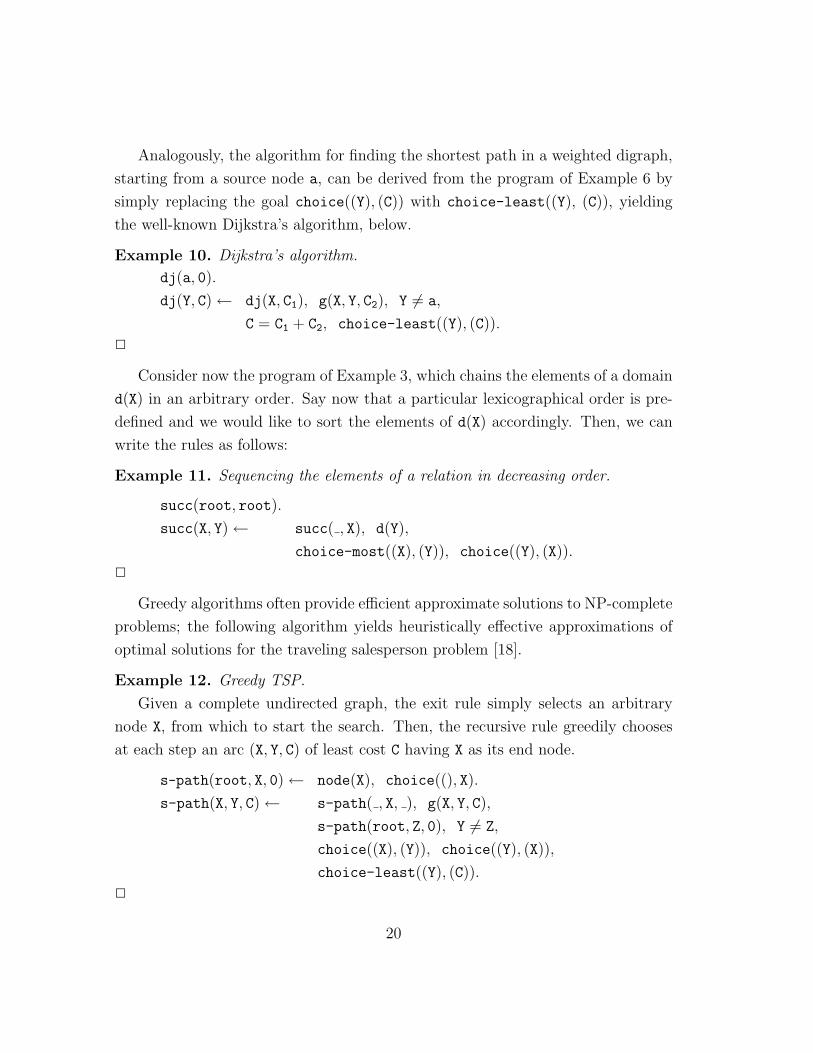
Analogously, the algorithm for finding the shortest path in a weighted digraph,

starting from a source node a, can be derived from the program of Example 6 by

simply replacing the goal choice((Y), (C)) with choice-least((Y), (C)), yielding

the well-known Dijkstra’s algorithm, below.

Example 10. Dijkstra’s algorithm.

dj(a, 0).

dj(Y, C) ← dj(X, C1), g(X, Y, C2), Y 6= a,

C = C1 + C2, choice-least((Y), (C)).

2

Consider now the program of Example 3, which chains the elements of a domain

d(X) in an arbitrary order. Say now that a particular lexicographical order is pre-

defined and we would like to sort the elements of d(X) accordingly. Then, we can

write the rules as follows:

Example 11. Sequencing the elements of a relation in decreasing order.

succ(root, root).

succ(X, Y) ← succ( , X), d(Y),

choice-most((X), (Y)), choice((Y), (X)).

2

Greedy algorithms often provide efficient approximate solutions to NP-complete

problems; the following algorithm yields heuristically effective approximations of

optimal solutions for the traveling salesperson problem [18].

Example 12. Greedy TSP.

Given a complete undirected graph, the exit rule simply selects an arbitrary

node X, from which to start the search. Then, the recursive rule greedily chooses

at each step an arc (X, Y, C) of least cost C having X as its end node.

s-path(root, X, 0) ← node(X), choice((), X).

s-path(X, Y, C) ← s-path( , X, ), g(X, Y, C),

s-path(root, Z, 0), Y 6= Z,

choice((X), (Y)), choice((Y), (X)),

choice-least((Y), (C)).

2

20

Observe that the program of Example 12 was obtained from that of Example

7 by replacing a choice goal with its choice-least counterpart.

Example 13. While we have here concentrated on graph optimization problems,

greedy algorithms are useful in a variety of other problems. For instance, in [8] we

discuss a greedy solution to the well-known knapsack problem consists in finding

a set of items whose total weight is lesser than a given value (say 100) and whose

cost is maximum. This is an NP-complete problem and, therefore, the optimal so-

lution requires an exponential time (assuming P 6= NP ); however, an approximate

solution can be found by means of a greedy computation, which selects at each

step the item with maximum value/weight ratio.

In conclusion, we have obtained a framework for deriving and expressing greedy

algorithms (such as Prim’s algorithm) characterized by conceptual simplicity, logic-

based semantics, and short and efficient programs; we can next turn to the efficient

implementation problem for our programs.

7 Implementation and Complexity

A most interesting aspect of the programs discussed in this paper is that their stable

models can be computed very efficiently. In the previous sections, we have seen

that the exponential intractability of stable models is not an issue here: our greedy

fixpoint computations are always polynomial-time in the size of the database. In

this section, we show that the same asymptotic complexity obtainable by expressing

the algorithms in procedural languages can be obtained by using comparable data

structures and taking advantage of syntactic structure of the program.

In general, the computation consists of two phases: (i) compilation and (ii)

execution. All compilation algorithms discussed here execute with time complexity

that is polynomial in the size of the programs. Moreover, we will assume, as it

is customarily done [29], that the size of the database dominates that of the pro-

gram. Thus, execution costs dominate the compilation costs, which can thus be

disregarded in the derivation of the worst case complexities. We will use compila-

tion techniques, such as the differential fixpoint computation, that are of common

21

usage in deductive database systems [29]. Also we will employ suitable storage

structures, such as hash tables to support search on keys, and priority queues to

support choice-least and choice-most goals.

We assume that our programs consist of a set of mutually recursive predicates.

General programs can be partitioned into a set of subprograms where rules in every

subprogram defines a set of mutually recursive predicates. Then, subprograms are

computed according to the topological order defined by the dependencies among

predicates, where tuples derived from the computation of a subprogram are used as

database facts in the computation of the subprograms that follow in the topological

order.

7.1 Implementation of Programs with Choice

Basically, the chosen atoms need to be memorized in a set of tables chosenr (one

for each chosenr predicate). The diffchoice atoms need not be computed and

stored; rather, a goal ¬diffchoicer(. . .) can simply be checked dynamically against

the table chosenr. We now present how programs with choice can be evaluated by

means of an example.

Example 14. Consider again Example 11

s1 : succ(root, root).

s2 : succ(X, Y) ← succ( , X), d(Y),

choice-most((X), (Y)), choice((Y), (X)).

2

According to our definitions, these rules are implemented as follows:

r1 : succ(root, root).

r2 : succ(X, Y) ← succ( , X), d(Y), chosen(X, Y).

r3 : chosen(X, Y) ← succ( , X), g(X, Y, C), ¬diffchoice(X, Y).r4 : diffchoice(X, Y) ← chosen(X, Y′), Y′ 6= Y.

r5 : diffchoice(X, Y) ← chosen(X′, Y), X′ 6= X.

22

(Strictly speaking, the chosen and diffchoice predicates should have been added

the subscript s2 for unique identification. But we dispensed with that, since there

is only one choice rule in the source program and no ambiguity can occur.) The

diffchoice rules are used to enforce the functional dependencies X → Y and Y → X

on the chosen tuples. These conditions can be enforced directly from the stored

table chosen(X, Y) by enforcing the following constraints 3:

← chosen(X, Y), chosen(X, Y′), Y′ 6= Y.

← chosen(X, Y), chosen(X′, Y), X′ 6= X.

that are equivalent to the two rules defining the predicate ¬diffchoice. Thus,

rules r4 and r5 are never executed directly, nor is any diffchoice atom ever gener-

ated or stored. Thus we can simply eliminate the diffchoice rules in the computation

of our program foe(P ) = PC ∪ PD. In addition, as previously observed, we can

eliminate the goal ¬diffchoice from the chosen rules without changing the defini-

tion of LICO (the Lazy Immediate-Consequence Operator introduced in Definition

4). Therefore, let P ′D denote PD after the elimination of the diffchoice rules, and let

P ′C denoted the rules in PC after the elimination of their negated diffchoice goals;

then, we can express our LICO computation as follows:

ΘI = {δ ∈ TP ′C (I) \ I | I ∪ {δ} |= FDP}Γlazy

P (I) = {I ∪ {δ} | δ ∈ ΘI} ∪ {I | ΘI = ∅}Ψlazy

P (I) = { T ↑ωP ′D

(J) | J ∈ ΓP (I) }

Various simplifications can be made to this formula. For program of Example

14, P ′D consists of the exit rule r1, which only needs to fired once, and of the rule

r2, where the variables in choice goals are the same as those contained in the head.

In this situation, the head predicate and the chosen predicate can be stored in the

same table and TP ′D is implemented at no additional cost as part of the computation

of chosen.

Consider now the implementation of a table chosenr. The keys for this table

are the left sides of the choice goals: X and Y for the example at hand. The data

structures needed to support search and insertion on keys are well-known. For main

3A constraint is a rule with empty head which is satisfied only if its body is false.

23

memory, we can use hash tables, where searching for a key value, and inserting or

deleting an entry can be considered constant-time operations. Chosen tuples are

stored into a table which can be accessed by means of a set of hash indexes. More

specifically, for each functional dependency X → Y there is an hash index on the

attributed specified by the variables in X.

7.2 Naive and Seminaive Implementations

For Example 14, the application of the LICO to the empty set, yields ΘI0 = ∅; then,

from the evaluation of the standard rules we get the set ΨlazyP (∅) = {p(nil, a)}.

At the next iteration, we compute ΘI1 and obtain all arcs leaving from node a.

One of these arcs is chosen and the others are discarded, as it should be since

they would otherwise violate the constraint X ↔ Y . This naive implementation

of Ψ generates no redundant computation for Example 14; similar considerations

also hold for the simple path program of Example 7. In many situations however,

tuples of ΘI computed in one iteration, also belong to ΘI in the next iteration,

and memorization is less expensive than recomputation. Symbolic differentiation

techniques similar to those used in the seminaive fixpoint computation, can be used

to implement this improvement [29], as described below.

We consider the general case, where a program can have more than one mutually

recursive choice rule and we need to use separate chosenr tables for each such rule.

For each choice rule r, we also store a table thetar with the same attributes as

chosenr. In thetar, we keep the tuples which are future candidates for the table

chosenr.

We update incrementally the content of the tables thetar as they were concrete

views, using differential techniques. In fact, Θr = θr t thetar, where thetar is the

table accumulation for the ‘old’ Θr tuples and θr is the set of ‘new’ Θr tuples

generated using the differential fixpoint techniques. Finally, ΘI in the LICO is

basically the union of the Θr for the various choice rules r.

With P ′C be the set of chosen rules in foe(P ), with the ¬diffchoice goal

removed; let Tr denote the immediate consequence operator for a rule r ∈ P ′C .

Also, P ′D will denote foe(P ) after the removal of the chosen rules and of the

diffchoice rules: thus P ′D is PD without the diffchoice rules.

24

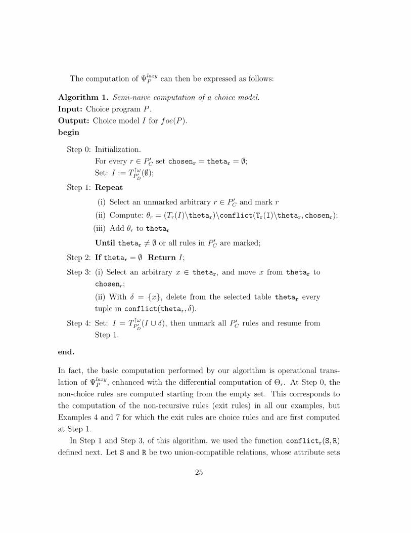
The computation of ΨlazyP can then be expressed as follows:

Algorithm 1. Semi-naive computation of a choice model.

Input: Choice program P .

Output: Choice model I for foe(P ).

begin

Step 0: Initialization.

For every r ∈ P ′C set chosenr = thetar = ∅;

Set: I := T ↑ωP ′D

(∅);Step 1: Repeat

(i) Select an unmarked arbitrary r ∈ P ′C and mark r

(ii) Compute: θr = (Tr(I)\thetar)\conflict(Tr(I)\thetar, chosenr);(iii) Add θr to thetar

Until thetar 6= ∅ or all rules in P ′C are marked;

Step 2: If thetar = ∅ Return I;

Step 3: (i) Select an arbitrary x ∈ thetar, and move x from thetar to

chosenr;

(ii) With δ = {x}, delete from the selected table thetar every

tuple in conflict(thetar, δ).

Step 4: Set: I = T ↑ωP ′D

(I ∪ δ), then unmark all P ′C rules and resume from

Step 1.

end.

In fact, the basic computation performed by our algorithm is operational trans-

lation of ΨlazyP , enhanced with the differential computation of Θr. At Step 0, the

non-choice rules are computed starting from the empty set. This corresponds to

the computation of the non-recursive rules (exit rules) in all our examples, but

Examples 4 and 7 for which the exit rules are choice rules and are first computed

at Step 1.

In Step 1 and Step 3, of this algorithm, we used the function conflictr(S, R)

defined next. Let S and R be two union-compatible relations, whose attribute sets

25

contain the left sides of the choice goals in r, i.e., the unique keys of chosenr (X

and Y for the example at hand). Then, conflictr(S, R) is the set of tuples in S

whose chosenr-key values are also contained in R.

Now, Step 1 brings up to date the content of the thetar table, while ensuring

that this does not contain any tuple conflicting with tuples in chosenr.

Symbolic differentiation techniques are used to improve the computation of

Tr(I) \ thetar in recursive rules at Step 1 (ii) [29]. This technique is particularly

simple to apply to a recursive linear rule where the symbolic differentiation yields

the same rule using, instead of the tuples of the whole predicate, the delta-tuples

computed in the last step. All our examples but Examples 7 and 12 involve linear

rule. The quadratic choice rule in Example 7 is differentiated into a pair of rules.

In all examples, the delta-tuples are as follows:

(i) The tuples produced by the exit rules at Step 0

(ii) The new tuples produced at Step 4 of the last iteration. For all our examples,

Step 4 is a trivial step where T ↑ωP ′D

(I ∪ δ) = I ∪ δ; thus δ is the new value produced

at Step 4.

Moreover, if r corresponds to a non-recursive, as the first rule in Examples 4

and 7, then this is only executed once with thetar = ∅.At Step 2, we check the termination condition, ΘI = ∅, i.e., Θr = ∅ for all r in

PC .

Step 3 (ii) eliminates from thetar all tuples that conflict with the tuple δ

(including the tuple itself).

Therefore, Algorithm 1 computes a stable model for foe(P ) since it imple-

ments a differential version of of the operator ΨlazyP , and applies this operator until

saturation.

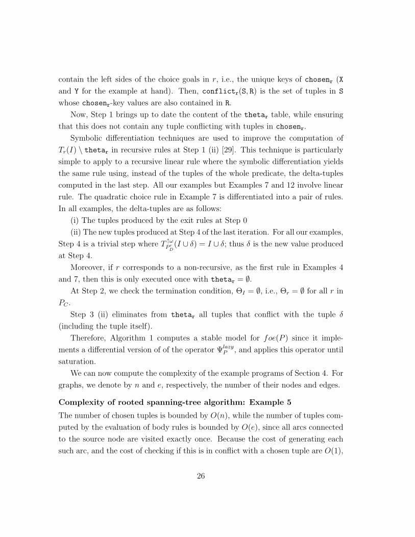
We can now compute the complexity of the example programs of Section 4. For

graphs, we denote by n and e, respectively, the number of their nodes and edges.

Complexity of rooted spanning-tree algorithm: Example 5

The number of chosen tuples is bounded by O(n), while the number of tuples com-

puted by the evaluation of body rules is bounded by O(e), since all arcs connected

to the source node are visited exactly once. Because the cost of generating each

such arc, and the cost of checking if this is in conflict with a chosen tuple are O(1),

26

the total cost is O(e).

Complexity of single-source reachability algorithm: Example 6

This case is very similar to the previous one. The size of reach is bounded by O(n),

and so is the size of the chosen and theta relations. However, in the process of

generating reach, all the edges reachable from the source node a are explored by

the algorithm exactly once. Thus the worst case complexity is O(e).

Complexity of simple path: Example 7

Again, all the edges in the graph will be visited in the worst case, yielding complex-

ity O(e), where e = n2, according to our assumption that the graph is complete.

Every arc is visited once and, therefore, the global complexity is O(e), with e = n2.

Complexity of a bipartite matching: Example 4

Initially all body tuples are inserted into the theta relation at cost O(e). The

computation terminates in O(min(n1, n2)) = O(n) steps, where n1 and n2 are,

respectively, the number of nodes in the left and right parts of the graph. At each

step, one tuple t is selected at cost O(1) and the tuples conflicting with the selected

tuple are deleted. The global cost of deleting conflicting tuples is O(e), since we

assume that each tuple is accessed in constant time. Therefore the global cost is

O(e).

Complexity of linear sequencing of the elements of a set: Example 3

If n is the cardinality of the domain d, the computation terminates in O(n) steps.

At each step, n tuples are computed, one tuple is chosen and the remaining tuples

are discarded. Therefore the complexity is O(n2).

7.3 Implementation of Choice-least/most Programs

In the presence of choice-least (or choice-most) goals, the best alternative must be

computed, rather than an arbitrary one chosen at random. Let us consider the

general case where programs could contain three different kinds of choice rules: (i)

choice-least rules that have one choice least goal, and zero or more choice goals,

(ii) choice-most rules that have one choice-most goal and zero or more choice goals,

27

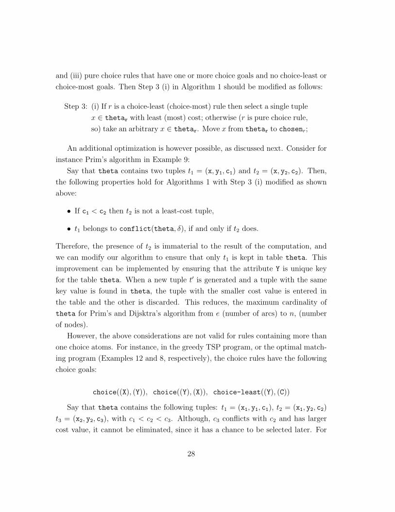
and (iii) pure choice rules that have one or more choice goals and no choice-least or

choice-most goals. Then Step 3 (i) in Algorithm 1 should be modified as follows:

Step 3: (i) If r is a choice-least (choice-most) rule then select a single tuple

x ∈ thetar with least (most) cost; otherwise (r is pure choice rule,

so) take an arbitrary x ∈ thetar. Move x from thetar to chosenr;

An additional optimization is however possible, as discussed next. Consider for

instance Prim’s algorithm in Example 9:

Say that theta contains two tuples t1 = (x, y1, c1) and t2 = (x, y2, c2). Then,

the following properties hold for Algorithms 1 with Step 3 (i) modified as shown

above:

• If c1 < c2 then t2 is not a least-cost tuple,

• t1 belongs to conflict(theta, δ), if and only if t2 does.

Therefore, the presence of t2 is immaterial to the result of the computation, and

we can modify our algorithm to ensure that only t1 is kept in table theta. This

improvement can be implemented by ensuring that the attribute Y is unique key

for the table theta. When a new tuple t′ is generated and a tuple with the same

key value is found in theta, the tuple with the smaller cost value is entered in

the table and the other is discarded. This reduces, the maximum cardinality of

theta for Prim’s and Dijsktra’s algorithm from e (number of arcs) to n, (number

of nodes).

However, the above considerations are not valid for rules containing more than

one choice atoms. For instance, in the greedy TSP program, or the optimal match-

ing program (Examples 12 and 8, respectively), the choice rules have the following

choice goals:

choice((X), (Y)), choice((Y), (X)), choice-least((Y), (C))

Say that theta contains the following tuples: t1 = (x1, y1, c1), t2 = (x1, y2, c2)

t3 = (x2, y2, c3), with c1 < c2 < c3. Although, c3 conflicts with c2 and has larger

cost value, it cannot be eliminated, since it has a chance to be selected later. For

28

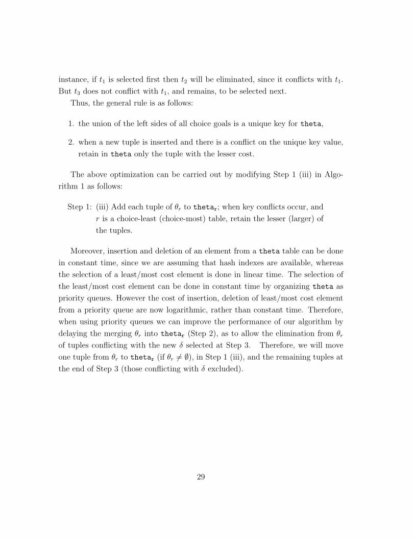
instance, if t1 is selected first then t2 will be eliminated, since it conflicts with t1.

But t3 does not conflict with t1, and remains, to be selected next.

Thus, the general rule is as follows:

1. the union of the left sides of all choice goals is a unique key for theta,

2. when a new tuple is inserted and there is a conflict on the unique key value,

retain in theta only the tuple with the lesser cost.

The above optimization can be carried out by modifying Step 1 (iii) in Algo-

rithm 1 as follows:

Step 1: (iii) Add each tuple of θr to thetar; when key conflicts occur, and

r is a choice-least (choice-most) table, retain the lesser (larger) of

the tuples.

Moreover, insertion and deletion of an element from a theta table can be done

in constant time, since we are assuming that hash indexes are available, whereas

the selection of a least/most cost element is done in linear time. The selection of

the least/most cost element can be done in constant time by organizing theta as

priority queues. However the cost of insertion, deletion of least/most cost element

from a priority queue are now logarithmic, rather than constant time. Therefore,

when using priority queues we can improve the performance of our algorithm by

delaying the merging θr into thetar (Step 2), as to allow the elimination from θr

of tuples conflicting with the new δ selected at Step 3. Therefore, we will move

one tuple from θr to thetar (if θr 6= ∅), in Step 1 (iii), and the remaining tuples at

the end of Step 3 (those conflicting with δ excluded).

29

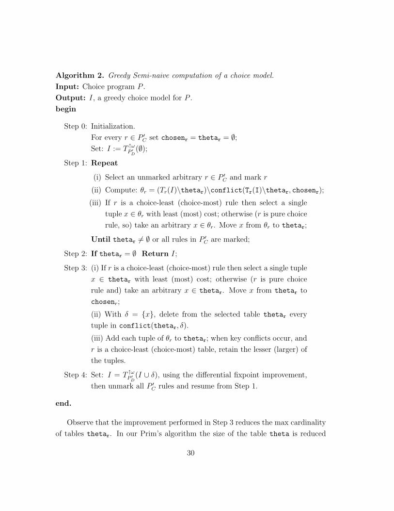
Algorithm 2. Greedy Semi-naive computation of a choice model.

Input: Choice program P .

Output: I, a greedy choice model for P .

begin

Step 0: Initialization.

For every r ∈ P ′C set chosenr = thetar = ∅;

Set: I := T ↑ωP ′D

(∅);Step 1: Repeat

(i) Select an unmarked arbitrary r ∈ P ′C and mark r

(ii) Compute: θr = (Tr(I)\thetar)\conflict(Tr(I)\thetar, chosenr);(iii) If r is a choice-least (choice-most) rule then select a single

tuple x ∈ θr with least (most) cost; otherwise (r is pure choice

rule, so) take an arbitrary x ∈ θr. Move x from θr to thetar;

Until thetar 6= ∅ or all rules in P ′C are marked;

Step 2: If thetar = ∅ Return I;

Step 3: (i) If r is a choice-least (choice-most) rule then select a single tuple

x ∈ thetar with least (most) cost; otherwise (r is pure choice

rule and) take an arbitrary x ∈ thetar. Move x from thetar to

chosenr;

(ii) With δ = {x}, delete from the selected table thetar every

tuple in conflict(thetar, δ).

(iii) Add each tuple of θr to thetar; when key conflicts occur, and

r is a choice-least (choice-most) table, retain the lesser (larger) of

the tuples.

Step 4: Set: I = T ↑ωP ′D

(I ∪ δ), using the differential fixpoint improvement,

then unmark all P ′C rules and resume from Step 1.

end.

Observe that the improvement performed in Step 3 reduces the max cardinality

of tables thetar. In our Prim’s algorithm the size of the table theta is reduced

30

from the number of edges e to the number of nodes n. This has a direct bearing

on the performance of our algorithm since the selection of a least cost tuple is

performed n times. Now, if a linear search is used to find the least-cost element

the global complexity is O(n×n). Similar considerations and complexity measures

hold for Dijsktra’s algorithm.

In some cases however, the unique key improvement just describe might be of

little or no benefit. For the TSP program and the optimal matching program,

where the combination of both end-points is the key for theta, no benefit is to

be gained since there is at most one edge between the two nodes. (In a database

environment this might follow from the declaration of unique keys in the schema,

and can thus be automatically detected by a compiler).

Next, we compute the complexity of the various algorithms, assuming that the

theta tables are supported by simple hash-based indexes, but there is no priority

queue. The complexities obtained with priority queues are discussed in the next

section.

Complexity of Prim’s Algorithm: Example 9

The computation terminates in O(n) steps. At each step, O(n) tuples are inserted

into the table theta, one least-cost tuple is moved to the table chosen and con-

flicting tuples are deleted from theta. Insertion and deletion of a tuple is done in

constant time, whereas selection of the least cost tuple is done in linear time. Since

the size of theta is bounded by O(n), the global complexity is O(n2).

Complexity of Dijkstra Algorithm: Example 10

The overall cost is O(n2) as for Prim’s algorithm.

Complexity of sorting the elements of a relation: Example 11

At each step, n candidates tuples are generated, one is chosen, and all tuples are

eliminated from theta. Here, each new X from succ is matched with every Y, even

when differential techniques are used. Therefore, the cost is O(n2).

Greedy TSP: Example 12

The number of steps is equal to n. At each step, n tuples are computed by the

evaluation of the body of the chosen rule and stored into the temporary relation

31

θ. Then, one tuple with least cost is selected (Step 1) and entered in theta all the

remaining tuples are deleted from the relation (Step 3). The cost of inserting one

tuple into the temporary relation is O(1). Therefore, the global cost is O(n2).

Optimal Matching in a directed graph: Example 8

Initially all body tuples are inserted into the theta relation at cost O(e). The

computation terminates in O(n) steps. At each step, one tuple t with least cost is

selected at cost O(e) and the tuples conflicting with the selected tuple are deleted.

The global cost of deleting conflicting tuples is O(e) (they are accessed in constant

time). Therefore the global cost is O(e× n).

7.4 Priority Queues

In many of the previous algorithms, the dominant cost is finding the least value in

the table thetar, where r is a least-choice or most-choice rule. Priority queues can

be used to reduce the overall cost.

A priority queue is a partially ordered tables where the cost of the ith element

is greater or equal than the cost of the (i div 2)th element [3]. Therefore, our table

thetar can be implemented as a list where each node having position i in the list

also contains (1) a pointer to the next element, (2) a pointer to the element with

position 2× i, and (3) a pointer to the element with position i div 2. The cost of

finding the least value is constant-time in a priority queue, the cost of adding or

deleting an element is log(m) where m is the number of the entries in the queue.

Also, in the implementation of Step 2 (ii), a linear search can be avoided by

adding one search index for each left side of a choice or choice-least goal. For

instance, for Dijkstra’s algorithm there should be a search index on X, for Prim’s

on Y . The operation of finding the least cost element in θr can be done during

the generation of the tuples at no additional cost. Then we obtain the following

complexities:

Complexity of Prim’s Algorithm: Example 9

The computation terminates in O(n) steps and the size of the priority queue is

bounded by O(n). The number of candidate tuples is bounded by O(e). Therefore,

the global cost is bounded by O(e× log n).

32

Complexity of Dijkstra Algorithm: Example 10

The overall cost is O(e× log n) as for Prim’s algorithm.

Complexity of sorting the elements of a relation: Example 11

The number of steps is equal to n. At each step, n tuples are computed, one is

stored into theta and next moved to chosen while all remaining tuples are deleted

from θ. The cost of each step is O(n) since deletion of a tuple from θ is constant

time. Therefore, the global cost is O(n2).

Greedy TSP: Example 12

Observe that thetar here contains at most one tuple. The addition of the first

tuple into an empty priority queue, thetar, and the deletion of the last tuple from

it are constant time operations. Thus the overall cost is the same as that without

a priority queue: i.e. the global cost is O(n2).

Optimal Matching in a bipartite graph: Example 8

Initially, all body tuples are inserted into the theta relation at cost O(e × log e).

The computation terminates in O(n) steps. At each step, one tuple t is selected

and all remaining tuples conflicting with t are deleted (the conflicting tuples here

are those arcs having the same node as source or end node of the arc). The

global number of extractions from the priority queue is O(e). Therefore, the global

complexity is O(e× log e).

Observe that, using a priority queues, an asymptotically optimum performance [3]

has been achieved for all problems, but that of sorting the elements of a domain,

Example 11. This problem is considered in the next section.

7.5 Discussion

A look at the structure of the program in Example 11 reveals that at the beginning

of each step a new set of (x, y) pairs is generated for theta by the two goals

succ( , X), d(Y) which define a Cartesian product. Thus, the computation can be

represented as follows:

Θ = π2succ× d

33

where succ and d are the relations containing their homonymous predicates. We

can also represent θ and theta as Cartesian products:

θ = (π2δ × d) \ chosen = π2δ × (d \ π2chosen)

Therefore, the key to obtaining an efficient implementation here consists in

storing only the second column of the theta relation, i.e.:

π2theta = d \ π2chosen

The operation of selecting a least-cost tuple from theta now reduces to that of

selecting a least-cost tuple from π2theta, which therefore should be implemented

as a priority queue.

Assuming these modifications, we can now recompute the complexity of our

Example 3, by observing that all the elements in d are added to π2theta once at

the first iteration. Then each successive iteration eliminates one element from this

set. Thus, the overall complexity is linear in the number of nodes. For Example

11, the complexity is O(n × log n) if we assume that a priority queue is kept for

π2theta Thus we obtain the optimal complexities.

No similar improvement is applicable to the other examples, where the rules

do not compute the Cartesian product of two relations. Thus, this additional

improvement could also be incorporated into a smart compiler, since it is possible

to detect from the rules whether theta is in fact the Cartesian product of its

two subprojections. However this is not the only alternative since many existing

deductive database systems provide the user with enough control to implement this,

and other differential improvements previously discussed, by coding them into the

program. For instance, the LDL++ users could use XY-stratified programs for

this purpose [28]; similar programs can be used in other systems [25].

8 Conclusion

This paper has introduced a logic-based approach for the design and implemen-

tation of greedy algorithms. In a nutshell, our design approach is as follows: (i)

formulate the all-answer solution for the problem at hand (e.g., find all the costs

34

of all paths from a source node to other nodes), (ii) use choice-induced FD con-

straints to restrict the original logic program to the non-deterministic generation

of a single answers (e.g., find a cost from the source node to each other node), and

(iii) specialize the choice goals with preference annotations to force a greedy heuris-

tics upon the generation of single answers in the choice-fixpoint algorithm (thus

computing the least-cost paths). This approach yields conceptual simplicity and

simple programs; in fact it has been observed that our programs are often similar

to the pseudo code used to express the same problem in a procedural language.

But our approach offers additional advantages, including a formal logic-based se-

mantics and a clear design method, supportable by a compiler, to achieve optimal

implementations for our greedy programs. This method is based on

• The use of chosen tables and theta tables, and of differential techniques to

support the second kind of table as a concrete view. The actual structure of

theta tables, their search keys and unique keys are determined by the choice

and choice-least goals, and the join dependencies implied by the structure of

the original rule.

• The use of priority queues for expediting the finding of extrema values.

Once these general guidelines are followed (by a user or a compiler) we obtain

an implementation that achieves the same asymptotic complexity as procedural

languages.

This paper provides a refined example of the power of Kowalski’s seminal idea:

algorithms = logic + control. Indeed, the logic-based approach here proposed covers

all aspects of greedy algorithms, including (i) their initial derivation using rules

with choice goals, (ii) their final formulation by choice-least/most goals, (iii) their

declarative stable-model semantics, (iv) their operational (fixpoint) semantics, and

finally (v) their optimal implementation by syntactically derived data structures

and indexing methods. This vertically integrated, logic-based, analysis and design

methodology represents a significant step forward with respect to previous logic-

based approaches to greedy algorithms (including those we have proposed in the

past [13, 7]).

35

Acknowledgement

The authors would like to thank D. Sacca for many hepfull discussions and sugges-

tions. The referees deserve credit for many improvements.

References

[1] Abiteboul S., R. Hull, V. Vianu. Foundations of Databases. Addison-Wesley.

1994.

[2] Abiteboul S. and V. Vianu. Datalog Extensions for Databases Queries and

Updates. In Journal of Computer and System Science, 43, pages 62–124, 1991.

[3] Aho A.V., J.E. Hopcropt J.E., and J.D. Ullman, The Design and analysis of

Computer Algorithms. Addison-Wesley, 1974.

[4] Apt K.R., H.A. Blair, and A. Walker. Towards a theory of declarative knowl-

edge. In (Minker ed.) Foundations of Deductive Databases and Logic Program-

ming, Morgan Kaufmann, 1988.

[5] Chandra A., and D. Harel, Structure and Complexity of Relational Queries,

Journal of Computer and System Sciences 25, 1, 1982, pp. 99-128.

[6] S. W. Dietrich. Shortest Path by Approximation in Logic Programs. ACM

Letters on Programming Lang. and Sys. Vol 1, No, 2, pages 119–137, June

1992.

[7] Ganguly S., S. Greco, and C. Zaniolo. Extrema Predicates in Deductive

Databases. Journal of Computer and System Science, 1995.

[8] S. Greco, and C. Zaniolo. Greedy Algorithms in Deductive Databases, UCLA

Technical Report, CSD-TR No 200002, February 2000.

[9] Gelfond M. and V. Lifschitz. The stable model semantics of logic programming.

In Proc. Fifth Intern. Conf. on Logic Programming, 1988.

[10] Giannotti F., D. Pedreschi, D. Sacca, and C. Zaniolo. Nondeterminism in

deductive databases. In Proc. 2nd DOOD Conference, 1991.

[11] Giannotti F., D. Pedreschi, C. Zaniolo, Semantics and Expressive Power of

Non-Deterministic Constructs in Deductive Databases, JCSS, to appear.

36

[12] Greco S., D. Sacca, and C. Zaniolo, DATALOG Queries with Stratified Nega-

tion and Choice: from P to DP In Proc. Fifth ICDT Conference, 81-96, 1995.

[13] Greco S., C. Zaniolo, and S. Ganguly. Greedy by Choice. In Proc. of the 11th

ACM Symp. on Principles of Database Systems, 1992.

[14] Greco S., and C. Zaniolo, Greedy Fixpoint Algorithms for Logic Programs

with Negation and Extrema. Technical Report, 1997.

[15] Krishnamurthy R. and S. Naqvi. Non-deterministic choice in Datalog. In Proc.

of the 3rd International Conf. on Data and Knowledge Bases, 1988.

[16] Marek W., M. Truszczynski. Autoepistemic Logic. Journal of ACM,

38(3):588–619, 1991.

[17] Moret B.M.E., and H.D. Shapiro. Algorithms from P to NP. Benjamin Cum-

mings, 1993.

[18] Papadimitriou C., K. Steiglitz, Combinatorial Optimization: Algorithms and

Complexity. Englewood Cliff, N.J., Prentice Hall.

[19] Przymusinski T., On the declarative and procedural semantics of stratified

deductive databases. In Minker, ed., Foundations of Deductive Databases and

Logic Programming, Morgan-Kaufman, 1988.

[20] A. Przymusinska and T. Przymusinski. Weakly Perfect Model Semantics for

Logic Programs. In Proceedings of the Fifth Intern. Conference on Logic Pro-

gramming, pages 1106–1122, 1988.

[21] K.A. Ross, and Y. Sagiv. Monotonic Aggregation in Deductive Databases. In

Proc. 11th ACM Symp. on Princ. of Database Systems, pages 127–138, 1992.

[22] Sacca D. and C. Zaniolo. Stable models and non-determinism in logic programs

with negation. Proc. Ninth ACM PODS Conference, 205–217, 1990.

[23] S. Sudarshan and R. Ramakrishnan. Aggregation and relevance in deductive

databases. In Proc. of the 17th Conference on Very Large Data Bases, 1991.

[24] Ullman J. D., Principles of Data and Knowledge-Base Systems. Vol 1 & 2,

Computer Science Press, New York, 1989.

37

[25] Vaghani J., K. Ramamohanarao, D. B. Kemp, Z. Somogyi, P. J. Stuckey, T.

S. Leask, and J. Harland. The Aditi deductive database system. The VLDB

Journal. Vol. 3(2), 245–288, 1994.

[26] Van Gelder A., K.A. Ross, and J.S. Schlipf. The well-founded semantics for

general logic programs. Journal of ACM, 38(3):620–650, 1991.

[27] Van Gelder A., Foundations of Aggregations in Deductive Databases In Proc.

of the Int. Conf. On Deductive and Object-Oriented databases, 1993.

[28] Zaniolo, C., N. Arni, K. Ong, Negation and Aggregates in Recursive Rules:

the LDL++ Approach, Proc. 3rd DOOD Conference, 1993.

[29] Zaniolo C., S. Ceri, C. Faloutsos, V.S. Subrahmanian and R. Zicari, Advanced

Database Systems, Morgan Kaufmann Publishers, 1997.

38