Gröbner Bases for Noncommutative Polynomialsamc/talks/grobner.pdfJJJNIII department of mathematics...

12

/ department of mathematics and computer scienceJJ J N I II 1/50JJ J N I II 1/50

Gröbner Bases for Noncommutative Polynomials

Arjeh M. Cohen

8 January 2007

first lecture ofThree aspects of exact computation

a tutorial atMathematics: Algorithms and Proofs (MAP)

Leiden, January 8–12, 2007

12


Outline

1. Introduction

2. Rewriting

3. Gröbner bases

4. Gröbner algorithm

5. Examples

6. Conclusion

Based on work with Dié Gijsbers

12


1. Introduction

Gröbner bases are generating sets of ideals incommutative polynomial rings k[x1, . . . , xn] that help

• solve polynomial systems of equation by triangularization

• solve linear equations over k[x1, . . . , xn] (ideal membership)

• describe quotient algebras effectively

The theory fails for non-commutative polynomial rings to a considerable extent,

but still there are things we can do.

12


Our concern

Finding Gröbner bases for finite generating sets of ideals

in noncommutative polynomial rings k〈x1, . . . , xn〉 that help

• describe quotient algebras effectively

12


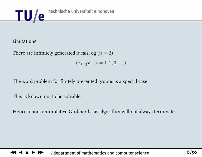
Limitations

There are infinitely generated ideals, eg (n = 2)

(x1xi2x1 : i = 1, 2, 3, . . .)

12


Limitations

There are infinitely generated ideals, eg (n = 2)

(x1xi2x1 : i = 1, 2, 3, . . .)

The word problem for finitely presented groups is a special case.

This is known not to be solvable.

Hence a noncommutative Gröbner basis algorithm will not always terminate.

12


Motivation by example

The transpositions r1 = (1, 2), r2 = (2, 3), and r3 = (3, 4) generate the symmetricgroup Σ4.

These satisfy the relations

r1r2r1 − r2r1r2 = 0

r2r3r2 − r3r2r3 = 0

r1r3 − r3r1 = 0

r21 − 1 = 0

r22 − 1 = 0

r23 − 1 = 0

In order to prove that this is a presentation of Σ4:get canonical forms for the 24 elements of Σ4 as words in r1 and r2.

12


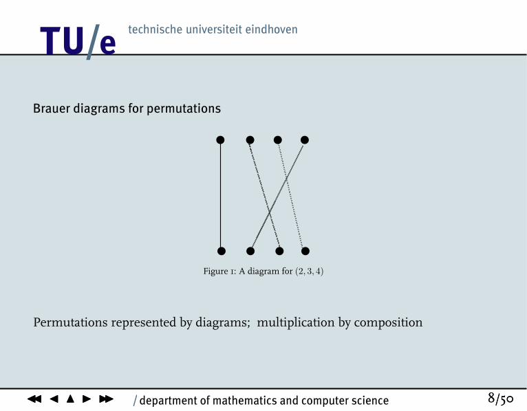
Brauer diagrams for permutations

x x x x

x x x xFigure 1: A diagram for (2, 3, 4)

Permutations represented by diagrams; multiplication by composition

12


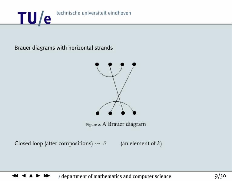
Brauer diagrams with horizontal strands

x x

x x

xx

xx

Figure 2: A Brauer diagram

Closed loop (after compositions) δ (an element of k)

12


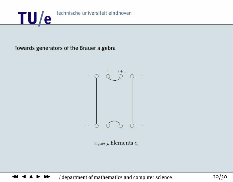
Towards generators of the Brauer algebra

hhhh

hhhh

i i + 1· · ·

· · ·· · ·

· · ·

Figure 3: Elements ei

12


Example

x x

x x

xx

xx

Figure 4: This Brauer diagram equals r2e1r3r2r3

12


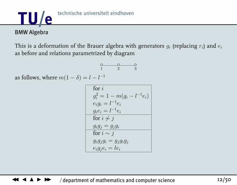
BMW Algebra

This is a deformation of the Brauer algebra with generators gi (replacing ri) and ei

as before and relations parametrized by diagram

◦1

◦2

◦3

as follows, where m(1 − δ) = l − l−1

for ig2

i = 1 −m(gi − l−1ei)eigi = l−1ei

giei = l−1ei

for i 6∼ j

gigj = gjgi

for i ∼ j

gigjgi = gjgigj

eigjei = lei

12


BMW algebra dimension

To compute the BMW algebra given by the above relations,find a Gröbner basis and compute dimension.

Input 17 polynomials (the relations) such ase1 − lm−1g2

1 − lg1 + lm−1 and g1g2g1 − g2g1g2

m = 7, l = 11. The computation took 350 msecs.

One of the 89 output polys: g1g2e3g2e1 + 7g2e3g2e1 − g2g3g2e1 + 7e3e2e1 + 49e3g2e1 +7e2e1e3 − 7g3g2e1 + 49g2e1e3 − 7g2g3e1 + 343e1e3 − 49g3e1 − 49g2e1 − 350e1

Dimension of the quotient algebra is 105 = 3 · 5 · 7.

Script done on Sun 07 Jan 2007 05:40:42 PM CET

12


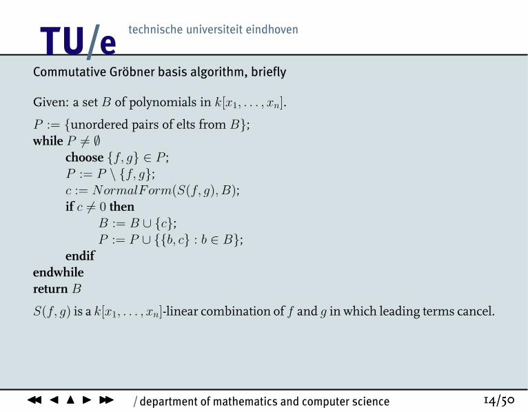
Commutative Gröbner basis algorithm, briefly

Given: a set B of polynomials in k[x1, . . . , xn].

P := {unordered pairs of elts from B};while P 6= ∅

choose {f, g} ∈ P ;P := P \ {f, g};c := NormalForm(S(f, g), B);if c 6= 0 then

B := B ∪ {c};P := P ∪ {{b, c} : b ∈ B};

endifendwhilereturn B

S(f, g) is a k[x1, . . . , xn]-linear combination of f and g in which leading terms cancel.

12


Commutative Gröbner basis algorithm, briefly

Given: a set B of polynomials in k[x1, . . . , xn].

P := {unordered pairs of elts from B};while P 6= ∅

choose {f, g} ∈ P ;P := P \ {f, g};c := NormalForm(S(f, g), B);if c 6= 0 then

B := B ∪ {c};P := P ∪ {{b, c} : b ∈ B};

endifendwhilereturn B

S(f, g) is a k[x1, . . . , xn]-linear combination of f and g in which leading terms cancel.

Termination: Ideal generated by L(B) increases and k[x1, . . . , xn] is Noetherian.

12


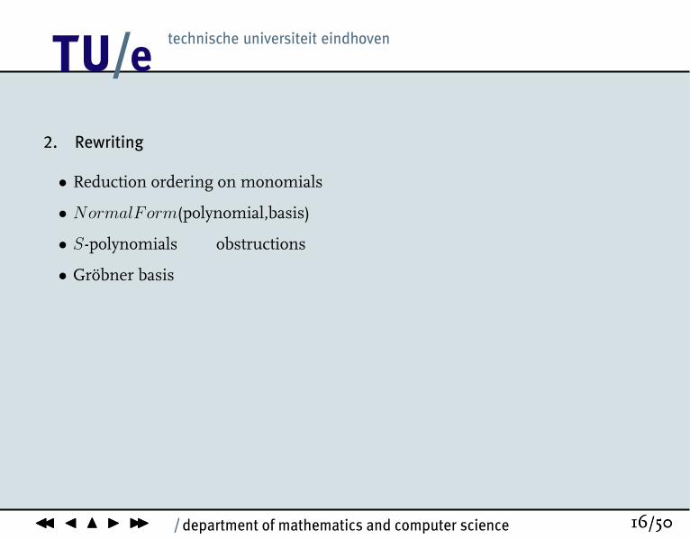
2. Rewriting

• Reduction ordering on monomials

• NormalForm(polynomial,basis)

• S-polynomials obstructions

• Gröbner basis

12


Reduction ordering

k is a field.

T is the free monoid on n generators x1, . . . , xn.

An ordering < on T is called a reduction orderingif, for all t1, t2, l, r ∈ T with t1 < t2,

1 ≤ lt1r < lt2r.

12


Examples

• lex(icographic) not a reduction orderingaj+1b < ajb conflicts with a > 1.

• deglex: total degree first, then lexicographic1 < a < b < a2 < ab < b2 < a3 < a2b < aba < ab2 < ba2 < bab < b2a < b3 < . . .

12


Reduction ordering, cont’d

Fix a reduction ordering < on T .

The reduction ordering is extensible to finite sets of monomials:A <F B iff A 6= B and ∀u ∈ A \B ∃ vv ∈ (B \ A) v > u.

deglex < is Noetherian andhence (by well known lemma) its extension <F .

12


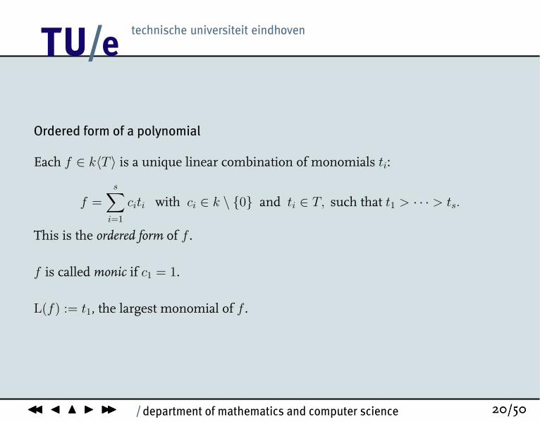
Ordered form of a polynomial

Each f ∈ k〈T 〉 is a unique linear combination of monomials ti:

f =s∑

i=1

citi with ci ∈ k \ {0} and ti ∈ T, such that t1 > · · · > ts.

This is the ordered form of f .

f is called monic if c1 = 1.

L(f) := t1, the largest monomial of f .

12


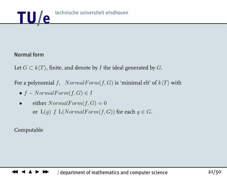
Normal form

Let G ⊂ k〈T 〉, finite, and denote by I the ideal generated by G.

For a polynomial f , NormalForm(f, G) is ‘minimal elt’ of k〈T 〉 with

• f −NormalForm(f, G) ∈ I

• either NormalForm(f, G) = 0

or L(g) 6 | L(NormalForm(f, G)) for each g ∈ G.

Computable

12


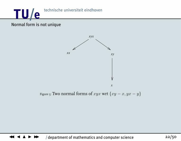
Normal form is not unique

xyx

xx xy

x

Figure 5: Two normal forms of xyx wrt {xy − x, yx − y}

12


3. Gröbner basis

A finite generating set G of an ideal I of k〈T 〉 is called a basis of I .

G is a Gröbner basis of I if

• G is a basis of I and

• NormalForm(h,G) = 0 for each h ∈ I .

12


Examples

G = [xy − x, yx − y]

NormalForm(s(1, 1, x; x, 2, 1), G) = x2 − x [xyx]

NormalForm(s(y, 1, 1; 1, 2, y), G) = y2 − y [yxy]

G ∪ [x2 − x, y2 − y] is a Gröbner basis.

12


Obstruction

Let G = (gi)1≤i≤k be a list of monic polynomials. An obstruction of G is a six-tuple

(l, i, r; λ, j, ρ)

with i, j ∈ {1, . . . , k} and l, λ, r, ρ ∈ T such that

L(gi) ≤ L(gj) and lL(gi)r = λL(gj)ρ.

S-polynomial

Given an obstruction we define the corresponding S-polynomial as

s(l, i, r; λ, j, ρ) = lgir − λgjρ.

12


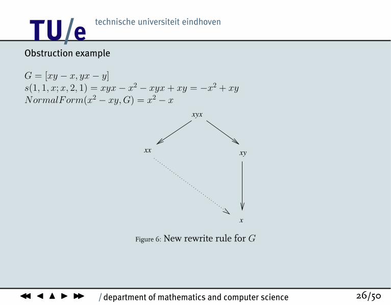
Obstruction example

G = [xy − x, yx − y]s(1, 1, x; x, 2, 1) = xyx− x2 − xyx + xy = −x2 + xy

NormalForm(x2 − xy,G) = x2 − x

xyx

xx xy

x

Figure 6: New rewrite rule for G

12


Reducing the number of obstructions

G = (gh) is a list of monic polynomials.A poly f is weak with respect to G if there are ch ∈ k and lh, rh ∈ T such that

f =∑

h

chlhghrh with lhL(gh)rh ≤ L(f).

We call an obstruction (l, i, r; λ, j, ρ) of G weak if its S-polynomial s(l, i, r; λ, j, ρ) isweak wrt G.

The S-polynomial of a weak obstruction (l, i, r; λ, j, ρ) can be written as follows withch ∈ k and lh, rh ∈ T .

s = lgir − λgjρ =∑

h

chlhghrh with lhL(gh)rh ≤ L(s) < lL(gi)r.

12


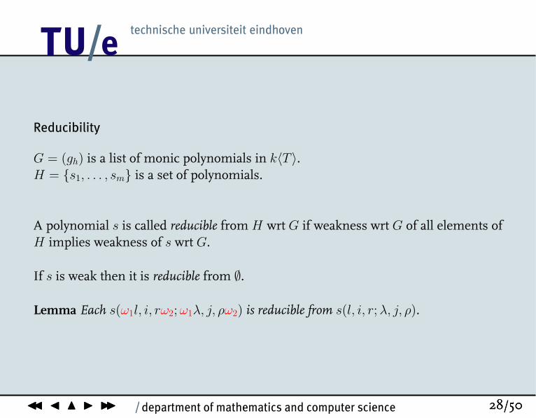
Reducibility

G = (gh) is a list of monic polynomials in k〈T 〉.H = {s1, . . . , sm} is a set of polynomials.

A polynomial s is called reducible from H wrt G if weakness wrt G of all elements ofH implies weakness of s wrt G.

If s is weak then it is reducible from ∅.

Lemma Each s(ω1l, i, rω2; ω1λ, j, ρω2) is reducible from s(l, i, r; λ, j, ρ).

12


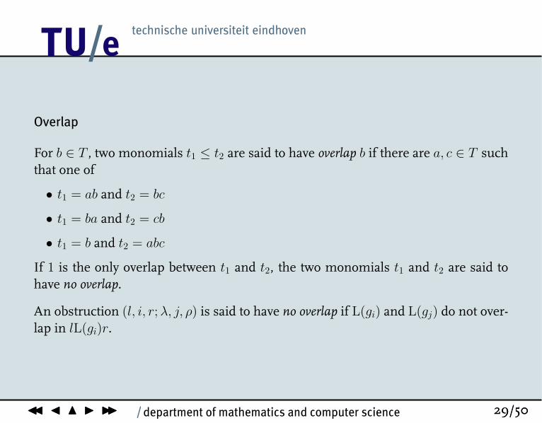
Overlap

For b ∈ T , two monomials t1 ≤ t2 are said to have overlap b if there are a, c ∈ T suchthat one of

• t1 = ab and t2 = bc

• t1 = ba and t2 = cb

• t1 = b and t2 = abc

If 1 is the only overlap between t1 and t2, the two monomials t1 and t2 are said tohave no overlap.

An obstruction (l, i, r; λ, j, ρ) is said to have no overlap if L(gi) and L(gj) do not over-lap in lL(gi)r.

12


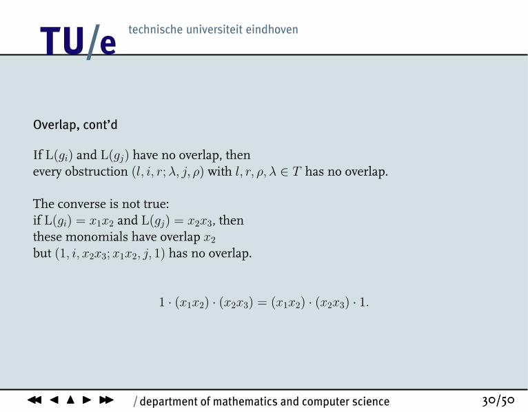
Overlap, cont’d

If L(gi) and L(gj) have no overlap, thenevery obstruction (l, i, r; λ, j, ρ) with l, r, ρ, λ ∈ T has no overlap.

The converse is not true:if L(gi) = x1x2 and L(gj) = x2x3, thenthese monomials have overlap x2

but (1, i, x2x3; x1x2, j, 1) has no overlap.

1 · (x1x2) · (x2x3) = (x1x2) · (x2x3) · 1.

12


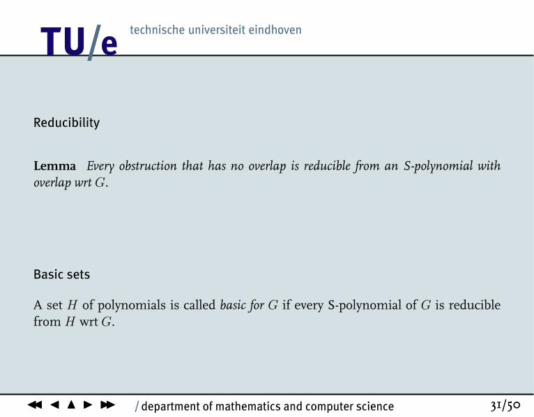
Reducibility

Lemma Every obstruction that has no overlap is reducible from an S-polynomial withoverlap wrt G.

Basic sets

A set H of polynomials is called basic for G if every S-polynomial of G is reduciblefrom H wrt G.

12


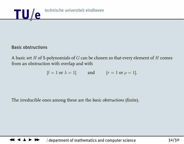
Basic obstructions

A basic set H of S-polynomials of G can be chosen so that every element of H comesfrom an obstruction with overlap and with

[l = 1 or λ = 1] and [r = 1 or ρ = 1].

The irreducible ones among these are the basic obstructions (finite).

12


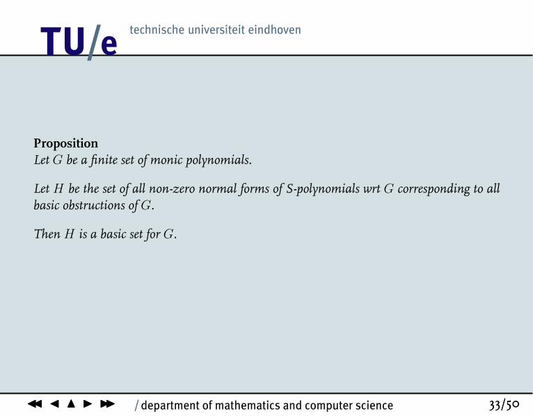
PropositionLet G be a finite set of monic polynomials.

Let H be the set of all non-zero normal forms of S-polynomials wrt G corresponding to allbasic obstructions of G.

Then H is a basic set for G.

12


Further trimming of the basic set

There are obstructions that can be removed from the list of those that need to beconsidered.

12


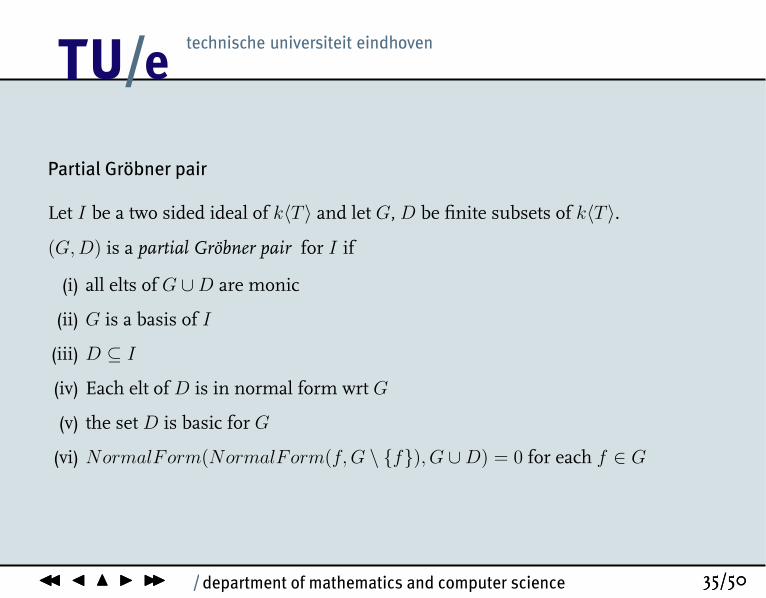
Partial Gröbner pair

Let I be a two sided ideal of k〈T 〉 and let G, D be finite subsets of k〈T 〉.

(G, D) is a partial Gröbner pair for I if

(i) all elts of G ∪D are monic

(ii) G is a basis of I

(iii) D ⊆ I

(iv) Each elt of D is in normal form wrt G

(v) the set D is basic for G

(vi) NormalForm(NormalForm(f, G \ {f}), G ∪D) = 0 for each f ∈ G

12


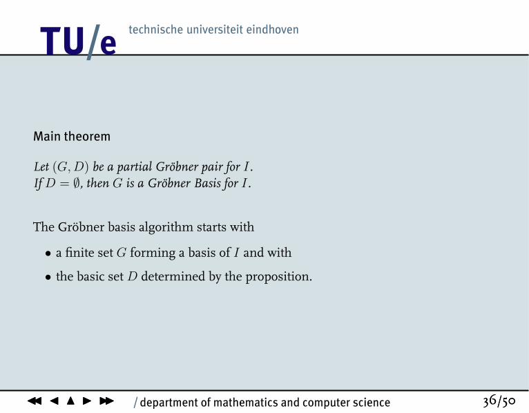
Main theorem

Let (G, D) be a partial Gröbner pair for I .If D = ∅, then G is a Gröbner Basis for I .

The Gröbner basis algorithm starts with

• a finite set G forming a basis of I and with

• the basic set D determined by the proposition.

12


4. Gröbner algorithm

Let (G, D) be a partial Gröbner pair for I . The four steps below compute a newpartial Gröbner pair (G′, D′) for I .

1. Move one polynomial f from D to G. Write G = {g1, . . . , gN−1, gN = f}.

2. Compute the basic obstructions b of G involving f . Update D with the non-zeroNormalForm(b, G ∪D). The new D is a basic set for the new G.

3. For each i ≤ N − 1 compute g′i = NormalForm(gi, G \ {gi}).If g′i = 0 remove gi from G. Otherwise, if g′i 6= gi,

(a) replace gi by g′i;

(b) compute the basic obstructions of the new G involving g′i;

(c) if NormalForm(b, G ∪D) 6= 0 for such an obstruction b, add it to D.

4. Replace each d ∈ D by NormalForm(d, (G ∪D) \ {d}.

12


Termination

Repeat the four steps until termination, if ever.

If D = ∅, then the routine terminates and G is a Gröbner basis for I .

k〈T 〉 is not Noetherian.

12


Dimensions of quotient algebras

Obtained by finding those monomials that are not contained in the order ideal ofleading terms of the Gröbner basis.

Example: Coxeter group of type W (E6) and order 51840

There exists a growth rate version.

12


5. Examples

G = [xy − x, yx − y]

NormalForm(s(1, 1, x; x, 2, 1), G) = x2 − x [xyx]

NormalForm(s(y, 1, 1; 1, 2, y), G) = y2 − y [yxy]

G ∪ [x2 − x, y2 − y] is a Gröbner basis.

12


Loading GBNP 0.9.2 (Non-commutative Gröbner bases)

G1 := [[[1,2],[1]],[1,-1]]; G2 := [[[2,1],[2]],[1,-1]];KI:=[G1,G2];

PrintNPList(KI);xy - x, yx - y

GB := SGrobnerTrace(KI); PrintNPListTrace(GB);x^2 - x, xy - x, yx - y, y^2 - y

PrintTraceList(GB);- G(1)x + G(1) + xG(2), G(1), G(2), yG(1) - G(2)y + G(2)

Script done on Wed 27 Dec 2006 02:56:18 PM CET

12


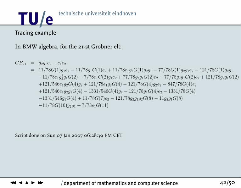
Tracing example

In BMW algebra, for the 21-st Gröbner elt:

GB21 = g2g1e2 − e1e2

= 11/78G(1)g1e2 − 11/78g1G(1)e2 + 11/78e1g2G(1)g2g1 − 77/78G(1)g2g1e2 − 121/78G(1)g2g1

−11/78e1g22g1G(2) − 7/78e1G(2)g1e2 + 77/78g2g1G(2)e2 − 77/78g2g1G(2)e2 + 121/78g2g1G(2)

+121/546e1g2G(4)g2 + 121/78e1g2G(4) − 121/78G(4)g2e2 − 847/78G(4)e2

+121/546e1g2g1G(4) − 1331/546G(4)g2 − 121/78g1G(4)e2 − 1331/78G(4)

−1331/546g1G(4) + 11/78G(7)e2 − 121/78g2g1g2G(8) − 11g2g1G(8)

−11/78G(10)g2g1 + 7/78e1G(11)

Script done on Sun 07 Jan 2007 06:28:39 PM CET

12


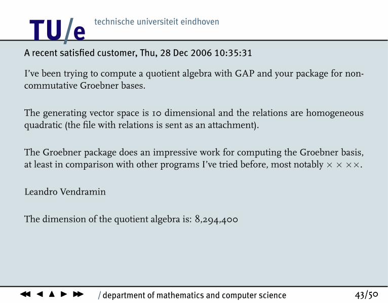
A recent satisfied customer, Thu, 28 Dec 2006 10:35:31

I’ve been trying to compute a quotient algebra with GAP and your package for non-commutative Groebner bases.

The generating vector space is 10 dimensional and the relations are homogeneousquadratic (the file with relations is sent as an attachment).

The Groebner package does an impressive work for computing the Groebner basis,at least in comparison with other programs I’ve tried before, most notably ××××.

Leandro Vendramin

The dimension of the quotient algebra is: 8,294,400

12


×××× ∈ {Bergman,Opal,Plural}\{GBNP }

12


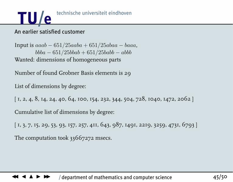
An earlier satisfied customer

Input is aaab− 651/25aaba + 651/25abaa− baaa,bbba− 651/25bbab + 651/25babb− abbb

Wanted: dimensions of homogeneous parts

Number of found Grobner Basis elements is 29

List of dimensions by degree:

[ 1, 2, 4, 8, 14, 24, 40, 64, 100, 154, 232, 344, 504, 728, 1040, 1472, 2062 ]

Cumulative list of dimensions by degree:

[ 1, 3, 7, 15, 29, 53, 93, 157, 257, 411, 643, 987, 1491, 2219, 3259, 4731, 6793 ]

The computation took 33667272 msecs.

12


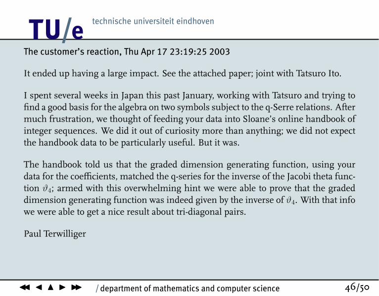
The customer’s reaction, Thu Apr 17 23:19:25 2003

It ended up having a large impact. See the attached paper; joint with Tatsuro Ito.

I spent several weeks in Japan this past January, working with Tatsuro and trying tofind a good basis for the algebra on two symbols subject to the q-Serre relations. Aftermuch frustration, we thought of feeding your data into Sloane’s online handbook ofinteger sequences. We did it out of curiosity more than anything; we did not expectthe handbook data to be particularly useful. But it was.

The handbook told us that the graded dimension generating function, using yourdata for the coefficients, matched the q-series for the inverse of the Jacobi theta func-tion ϑ4; armed with this overwhelming hint we were able to prove that the gradeddimension generating function was indeed given by the inverse of ϑ4. With that infowe were able to get a nice result about tri-diagonal pairs.

Paul Terwilliger

12


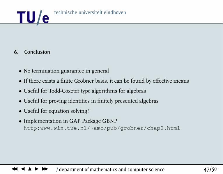
6. Conclusion

• No termination guarantee in general

• If there exists a finite Gröbner basis, it can be found by effective means

• Useful for Todd-Coxeter type algorithms for algebras

• Useful for proving identities in finitely presented algebras

• Useful for equation solving?

• Implementation in GAP Package GBNPhttp:www.win.tue.nl/~amc/pub/grobner/chap0.html

12


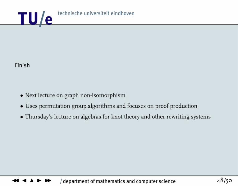
Finish

• Next lecture on graph non-isomorphism

• Uses permutation group algorithms and focuses on proof production

• Thursday’s lecture on algebras for knot theory and other rewriting systems

12


12


References

[1] A.M. Cohen & D.A.H. Gijsbers, Noncommutative Groebner basis computa-tions, GBNP, Eindhoven 2003http://www.win.tue.nl/~amc/pub/grobner/doc.html .

[2] Edward L. Green, Noncommutative Grobner bases, and projective resolutions,pp. 29-60 in "Computational Methods for Representations of groups and alge-bras (Essen 1997), Birkhauser, Basel 1999.

[3] C. Krook, Dimensionality of quotient algebras, Eindhoven (2003).

[4] S.A. Linton, On vector enumeration, Linear Algebra Appl., 192 (1993) 235–248(Computational linear algebra in algebraic and related problems (Essen, 1992)).

[5] Theo Mora, An introduction to commutative and non-commutative GröbnerBases, Theoretical Computer Science, 134 (1994) 131–173.

[6] V.A. Ufnarovskii, On the use of graphs for calculating the basis, growth andHilbert series of associative algebras, Mat. Sb., 180 (11) (1989) 1548–1560, 1584.

Gröbner Bases for Noncommutative Polynomialsamc/talks/grobner.pdfJJJNIII department of mathematics...

Documents

Transcript of Gröbner Bases for Noncommutative Polynomialsamc/talks/grobner.pdfJJJNIII department of mathematics...