Gravity Recovery and Climate...

GRACE 327-734(CSR-GR-03-01)

Gravity Recovery and Climate Experiment

Level-2 Gravity Field ProductUser Handbook

(Rev 1.0, December 1, 2003 – Draft)

Srinivas BettadpurCenter for Space Research

The University of Texas at Austin

GRACE L-2 Product User Manual CSR-GR-03-01GRACE 327-734 (v 1.0 draft) December 1, 2003 Page 1 of 17

Prepared by:

_____________________________________________Srinivas Bettadpur, UTCSRGRACE Science Operations Manager

Contact Information:Center for Space ResearchThe University of Texas at Austin3925 W. Braker Lane, Suite 200Austin, Texas 78759-5321, USAEmail: [email protected]

Reviewers:

Frank Flechtner, Deputy Science Operations ManagerGeoForschungsZentrum, Potsdam

Paul Thompson,Center for Space Research, Austin

John Wahr, Member GRACE Science TeamUniversity of Colorado, Boulder

Michael M. Watkins, GRACE Project ScientistJet Propulsion Laboratory, CA

Victor Zlotnicki, Member GRACE Science TeamJet Propulsion Laboratory, CA

Approved by:

__________________________Byron D. TapleyGRACE Principal Investigator

___________________________Christoph ReigberGRACE Co-Principal Investigator


DOCUMENT CHANGE RECORD

Issue Date Pages Change Description1.0 Dec 1, 2003 All First Version 1.0 - DRAFT


TABLE OF CONTENTS

DOCUMENT CHANGE RECORD .................................................................................................................. 2

TABLE OF CONTENTS .................................................................................................................................... 3

I BACKGROUND ........................................................................................................................................ 4

I. 1 PURPOSE OF THE HANDBOOK ..................................................................................................................... 4I. 2 GRACE MISSION........................................................................................................................................ 4I. 3 THE GEOPOTENTIAL.................................................................................................................................... 4I. 4 NORMALIZATION CONVENTIONS................................................................................................................ 5I. 5 COMPONENT VARIATIONS .......................................................................................................................... 6

II GEOPOTENTIAL ESTIMATES ............................................................................................................ 7

II. 1 INTRODUCTION........................................................................................................................................... 7II. 2 BACKGROUND GRAVITY MODELS............................................................................................................. 7

II.2.1 Mixed Resolution of Background Models .................................................................................... 8II. 3 PARAMETRIZATION OF GEOPOTENTIAL ESTIMATE................................................................................... 9

II.3.1 The Geopotential Product........................................................................................................... 11II.3.2 Epochs Associated With the Geopotential Product ................................................................... 11

II. 4 THE AVERAGE GEOPOTENTIAL ............................................................................................................... 11II.4.1 Interpreting Product Variability................................................................................................. 12

III GRACE LEVEL-2 PRODUCTS....................................................................................................... 14

III. 1 PRODUCT INDENTIFIER........................................................................................................................... 14III. 2 PRODUCT CONTENTS.............................................................................................................................. 15

III.2.1 Defining Constants................................................................................................................. 15III.2.2 Product Span and Epoch ....................................................................................................... 15III.2.3 Calibration Coefficients for Uncertainties............................................................................ 16III.2.4 Companion Documents.......................................................................................................... 16

REFERENCES................................................................................................................................................... 17


I BACKGROUND

I. 1 PURPOSE OF THE HANDBOOK

The GRACE Level-2 Gravity Field Product User Handbook provides a description of theEarth gravity field estimates provided by the Level-2 processing. In particular, therelationship of the abstract concept of the geopotential (i.e. Earth’s gravity field and itsvariations), its instantaneous and mean values, and the specific set of GRACE gravityestimates (i.e. GRACE gravity field products) is elaborated.

I. 2 GRACE MISSION

The primary objective of the GRACE mission is to obtain accurate estimates of the meanand time-variable components of the Earth’s gravity field variations, for a period of fiveyears. This objective is achieved by making continuous measurements of the change indistance between twin spacecraft, co-orbiting in ≈ 500 km altitude, near circular, polarorbit, spaced ≈ 220 km apart, using a microwave ranging system. In addition to thisrange change, the non-gravitational forces are measured on each satellite using a high-accuracy electrostatic, room-temperature accelerometer. The satellite orientation andposition (& timing) are precisely measured using twin star cameras and a GPS receiver,respectively.

Spatial and temporal variations in the Earth’s gravity field affect the orbits (ortrajectories) of the twin spacecraft differently. These differences are manifested aschanges in the distance between the spacecraft, as they orbit the Earth. This change indistance is reflected in the time-of-flight of microwave signals transmitted and receivednearly simultaneously between the two spacecraft. The change in this time of flight iscontinuously measured by tracking the phase of the microwave carrier signals. The so-called dual-one-way range change measurements can be reconstructed from these phasemeasurements. This range change (or its numerically derived derivatives), along withother mission and ancillary data, is subsequently analyzed to extract the parameters of anEarth gravity field model.

I. 3 THE GEOPOTENTIAL

The word “geopotential” in this document will refer to the exterior potential of the Earthsystem, which includes its entire solid and fluid (including oceans and atmosphere)components. Following conventional methods (Heiskanen & Moritz 1966), at a fieldpoint P, exterior to the Earth system, the potential of gravitational attraction between aunit mass and the Earth system may be represented using an infinite spherical harmonicseries. The field point P is specified by its geocentric radius r, geographic latitude

†

j , andlongitude l. If m represents the gravitational constant of the Earth, and ae represents its


mean equatorial radius (or a scale distance), then the Earth’s exterior potential (orgeopotential, as used in this document) can be represented as

†

V (r,j,l;t)=mr

+mr

ae

rÊ

Ë Á

ˆ

¯ ˜

l= 2

Nmax

Âl

P lm (sinj) C lm (t)cosl + S lm (t)sinl{ }m= 0

l

Â (1)

In this expression,

†

P lm sinj( ) are the (fully-normalized) Associated LegendrePolynomials of degree l and order m; and

†

C lm and

†

S lm are the (fully-normalized)spherical harmonic coefficients of the geopotential.

The geopotential at a fixed location is variable in time due to mass movement andexchange between the Earth system components. This is reflected by introducing theindependent variable time (t) on the left; and is implemented or realized by treating thespherical harmonic coefficients of the geopotential as time dependent. The continuum ofvariations of the geopotential is represented by theoretically continuous variation of thegeopotential coefficients.

Though the spherical harmonic expansion of the geopotential requires an infinite series ofharmonics, practicality dictates that the summation on the right be limited to a maximumdegree Nmax.

In satellite geodetic convention, the origin of the reference frame is chosen to becoincident with the center of mass of the entire Earth system, including its solidcomponent and fluid envelopes. In this convention, the potential has no terms of degreel=1 on the right hand side of Eq. 1.

I. 4 NORMALIZATION CONVENTIONS

If

†

j denotes the geographical latitude of a field point (0° at equator, 90° at the Northpole, and –90° at the South pole), and if

†

u = sinj , then the un-normalized LegendrePolynomial of degree l is defined by

†

Pl (u) =1

2l ¥ l!¥

dl

dul u2 -1( )l

The definition of the un-normalized Associated Legendre Polynomial is then

†

Plm (u) = 1- u2( )m2 dm

dum Pl (u)

If the normalization factor is defined such that


†

Nlm2 =

(2 -d0m )(2l +1)(l - m)!(l + m)!

and the Associated Legendre Polynomials are normalized by

†

P lm = NlmPlm

then, over a unit sphere S

†

P lm (sinj)cosml

sinml

Ï Ì Ó

¸ ˝ ˛

È

Î Í

˘

˚ ˙

2

SÚ dS = 4p (2)

In this convention, the relationship of the spherical harmonic coefficients to the massdistribution becomes

†

C lmS lm

Ï Ì Ó

¸ ˝ ˛

=1

(2l +1)Me

¥¢ r

ae

Ê

Ë Á

ˆ

¯ ˜

GlobalÚÚÚ

l

P lm (sin ¢ j )cosm ¢ l

sinm ¢ l

Ï Ì Ó

¸ ˝ ˛

dM (3)

where

†

¢ r ,

†

¢ j and

†

¢ l are the coordinates of the mass element dM in the integrand. Theintegration is carried out over the entire mass envelope of the Earth system, including itssolid and fluid components.

This convention is consistent with the definition of fully-normalized harmonics in NRC(1997), and textbooks such as Heiskanen and Moritz (1966), Torge (1980); as well as inearlier gravity field models such as EGM96.

I. 5 COMPONENT VARIATIONS

At several places in this document, the total geopotential, as quantified by a set of total,time-dependent spherical harmonic coefficients, is separated into its componentvariations. Each component might represent one or more parts of the total Earth system(e.g. atmospheric or oceanic variations), or might represent a specific geophysicalphenomenon (e.g. solid Earth tides).

Such separate components are used in a linearly additive manner in all of GRACE dataanalysis. In particular, if a component has for its domain only a part of the Earth system,then the coefficients for that phenomenon represent the contribution to the exteriorgeopotential from an integration carried over a limited spatial domain in Eq. 3.


II GEOPOTENTIAL ESTIMATES

II. 1 INTRODUCTION

An instantaneous measurement of biased-range, or its derivatives, from the GRACEinstruments suite, is directly related to the instantaneous position and velocity (ortrajectory) of the GRACE spacecraft. The GRACE spacecraft trajectories contain theinfluence of the total exterior geopotential (and other forces) on each GRACE satellite.In the GRACE data analysis, the mathematical model for this dependence is thedynamical equations of motion for each satellite,

†

r ˙ ̇ r A =r f A ; r ˙ ̇ r B =

r f B (4)

where the subscripts A and B denote the two GRACE satellites,

†

r r is the position vectorin an Earth-centered inertial frame; and the right hand side is the sum of gravitational andnon-gravitational accelerations acting on each satellite.

In principle, therefore, a collection of biased range measurements, over a suitable timespan, with suitable or sufficient geographical coverage, and properly corrected for non-gravitational effects, is implicitly representative of the exterior gravity field of the Earthand its variations within that time span.

In GRACE science processing, this implicit relationship is parametrized in a specificway, and estimates of the geopotential parameters are determined from this selected dataspan. These estimates represent both improvements to the existing models for the Earth’sgravitational variations as well as new information on previously un-modeled gravityvariations due to various geophysical phenomena. This concept is elaborated in thefollowing sections.

II. 2 BACKGROUND GRAVITY MODELS

In each processing of the GRACE science data, estimates are made of updates to an apriori best-known geopotential model. This a priori gravity model is a part of the so-called Background Model. This approach is used for several reasons. The iterative,linearized least squares approach to the solution of an essentially non-linear problem isbetter behaved (in the sense of convergence) if the linearized updates are small, which isassured by using comprehensive background gravity models. Furthermore, due to orbitaltrack coverage limitations, rapid variability in the gravity field cannot be well determinedfrom GRACE data, though, if neglected, it has the potential to corrupt the GRACEestimate through aliasing. Finally, some geophysical models of variability can be betterdetermined from other techniques besides GRACE, in which case it is beneficial toremove such signals from the background using the best available external knowledge.


The Background Model consists of mathematical models and the associated parametervalues, which are used along with numerical techniques to predict a best-known value forthe observable (in this case, the inter-satellite range or its derivatives). The BackgroundModel encompasses both satellite dynamics and measurements. This model may beexpected to change with the evolution of processing methods – and is described in detailin the respective Level-2 Processing Standards Documents.

Since the geopotential is parametrized as a set of spherical harmonic coefficients, let G(t)represent the value of any coefficient set at epoch t. The Background Gravity Modelvalue may then be written as

†

G*(t) = G * + ¢ G (t - t0) + dGst (t) + dGot (t) + dG pt (t) + dGa +o(t) (5)

The first term

†

G * represents the a priori best knowledge of the static (or long-term mean)geopotential. It represents most of the non-spherical gravitational forces acting on thesatellite, and in the past has been represented by models such as EGM96. It is possiblefor this to be one of the previously derived GRACE gravity field products, though it isnot required to be so.

The remaining terms in Eq. (5) represent the a priori best knowledge of the variations inthe gravity field of the Earth. The second term represents the secular variations of theharmonics; the third, fourth and fifth terms represent the solid, ocean & pole tides,respectively. The last term a combination of atmospheric and oceanic non-tidalvariability.

The background gravity model used for data processing differs from the true gravity fieldof the Earth in two ways – by errors of omission of either certain geophysical phenomenaor spatial components; and by errors of commission by having incorrect models orparameter values for certain other phenomena.

II.2.1 Mixed Resolution of Background Models

It is noted that each of the component background models has its own inherent resolutionin time and space. Thus, the secular rates are available and significant for only the lowestdegree harmonics. The body-tides and ocean-tides are semi-analytic functions – wherethe variations occur at discrete & well-known frequencies, and are calculable at anyarbitrary epoch, but have empirically determined amplitudes at variable spatialresolutions. The pole-tides have the resolution of the polar-motion time series and areevaluated at intermediate epochs by suitable interpolation. The non-tidal atmosphere andoceans have different resolution in time and space, and must be similarly interpolated atintermediate epochs. An example of the component variations over three arbitrarilyselected days is shown in Figure 1.


-5 10-10

0 100

5 10-10

1 10-9

52487 52487.5 52488 52488.5 52489 52489.5 52490

totalsolid tides (analytic)ocean tides (analytic)non-tidal atm+ocean (6hr time-series)secular change (analytic)

dC20

(t)

Time (modified Julian date)

Figure 1 Components of the background model contributions to the C20 harmonic.

II. 3 PARAMETRIZATION OF GEOPOTENTIAL ESTIMATE

The collection of background models is used in GRACE data processing to make aprediction of the observable range change (or its derivatives). The difference between theobserved and predicted values of the measurements is the residual, which exists becauseof the aforementioned errors of omission & commission, in addition to the measurementerrors and model deficiencies. The background gravity model errors may be expected tohave continuum spatio-temporal variability. An update to the background gravity modelis to be computed such that the measurement residuals are minimized in the least-squaressense – and this update may be regarded as the new gravity information available fromGRACE.

In GRACE science data processing, at the most elementary level, this update to thegeopotential is parametrized, for a selected data span, as a set of constant corrections tothe spherical harmonic coefficients of the geopotential, to a specified maximum degreeand order. Functionally, this may be represented as

†

d ˆ G (Ts) = L Yi - f G*(ti)( ),i =1,...,m{ } (6)


In this equation, the left hand side represents a set of geopotential parameters estimatedfrom a specific data span

†

Ts ; L stands for the linearized least squares problem solved toobtain this estimate, using a collection of m observation residuals within that data span.For the specific coefficient

†

C 20 , the situation is depicted pictorially in Figure 2.

-3 10-9

-2 10-9

-1 10-9

0 100

1 10-9

2 10-9

52485 52490 52495 52500 52505 52510 52515 52520

dC20 (t) - time series used for background

average of background variability ( ≈ 4.6141E-11 )the update from estimation ( ≈ 1.2414E-10 )

dC20

(t)

Time (modified Julian date)

Gaps indicate that data werenot used in estimation

Figure 2 Depiction of the background model and its update from a GRACEsolution.

In this way, the long term variability of the geopotential relative to the adoptedbackground gravity model is traced by a sequence of piece-wise constant (or comparable)spherical harmonic coefficient sets over a specific duration – generally on the order ofone month. Note in Figure 2 that not every data point within the span may have beenused for the estimation of the constant update to the geopotential – even though theestimate is said to be valid over a data span bound by its end points.

As stated before, the sequence of such GRACE derived gravity estimates represent notonly the corrections to the existing models for the Earth’s gravitational variations, butalso new information on previously un-modeled gravity variations due to variousgeophysical phenomena


II.3.1 The Geopotential Product

For several applications, it is useful to regard the estimate

†

d ˆ G (Ts) as an update orcorrection to the background static geopotential model. This is also consistent withhistorical practice in geodesy. For this reason, both

†

d ˆ G (Ts) as well as the quantity

†

˜ G (Ts) = G * + d ˆ G (Ts) (7)

are to be regarded as GRACE data products – and this distinction is clear in the productnomenclature. Either of these products represents corrections to errors of commission oromissions from the background gravity models, and represents equally the new gravityinformation available from GRACE for scientific analysis.

II.3.2 Epochs Associated With the Geopotential Product

In general, there is no single epoch that can be perfectly associated with the GRACELevel-2 gravity field product. The start and the stop times for the data span

†

Ts areprovided along with the coefficients values as a part of the Level-2 products. Theestimates for any one span may be treated as corrections to the average of the backgroundgravity model for that span. If it is necessary to associate a gravity field estimate with asingle epoch, the mid-point of the data span used in the solution may be adopted.

II. 4 THE AVERAGE GEOPOTENTIAL

As is evident from previous discussions, for the data span

†

Ts , the total geopotential isrepresented as a heterogeneous mix between the background gravity model and thegeopotential estimate update. In particular, orbital dynamics and the estimation processare necessarily non-linear, so that the changes in the background gravity models do notnecessarily connect linearly to changes in the estimated piece-wise constant updates tothe geopotential.

Nevertheless, to some approximation and particularly for small variations, it is possible torelate the averages of background gravity models and the estimate updates. Define thetime-average of the geopotential coefficients by

†

G Ts ≡1Ts

G(t )dtTs

Ú (8)


Recalling Eq. 5, over the specific data span

†

Ts , let

†

eGbgo

Ts represent the average of the

errors of omission in the background gravity model; let

†

eGbgc

Ts represent the average ofthe errors of commission in the background gravity model; and let

†

eG * represent theerrors in the background mean or static gravity field.

Then the best estimate of the geopotential update from GRACE data processing over thetime-span

†

Ts may be written as

†

d ˆ G (Ts) ª eGbgo

Ts+ eGbg

c

Ts+ eG * (9)

The expression does not use an equality operator as the two sides differ by the estimationerrors in GRACE data processing.

II.4.1 Interpreting Product Variability

Let the best estimates for two different data spans TA and TB be written as

†

d ˆ G (TA ) ª eGbgo

TA+ eGbg

c

TA+ eG *

d ˆ G (TB ) ª eGbgo

TB + eGbgc

TB + eG *(10)

This pair of equations provides a possible basis for interpretation of a sequence ofGRACE products as time variable signals in the Earth gravity field, to within thecombined errors of estimation from the two data spans.

If one assumes that the background gravity models are perfect except for errors ofomissions, (i.e. errors of commission are zero), the difference between GRACE productsfrom two different data spans is interpretable as the change in the average of the gravitysignals due to the omitted variability effects. In that case,

†

d ˆ G (TA ) -d ˆ G (TB ) = eGbgo

TA- eGbg

o

TB (11a)

If some or all of the background gravity model components are deemed imperfect (i.e.errors of both omission & commission are non-zero), then the estimate differencesadditionally reflect the change in the average of the errors of commission between thetwo data spans. In this case,

†

d ˆ G (TA ) -d ˆ G (TB ) ª eGbgc

TA- eGbg

c

TB

+ eGbgo

TB - eGbgo

TA(11b)


Note that, in general, no frequency domain filtering is done on the input backgroundmodels. Thus the GRACE estimate updates reflect the averages of the omission andcommission error signals with the complete frequency bandwidth of the phenomena.

This discussion also provides a guide if the user wishes to mimic approximately theeffects of replacing a component of the background model on the variability evident inthe GRACE products. Nominally, the estimate for any one span is an update relative tothe average of the background gravity model. The replacement background gravitymodel may not be expected to have the same average. In this case, the right-hand sidemust have an additional term that takes into account the difference of the averages of theoriginal and replacement background model over the two data spans.

The GRACE product taxonomy has been developed to accommodate the definitions andcombinations described in this section. The preceding discussion is applicable to bothforms of the product described in II.3.1.


III GRACE LEVEL-2 PRODUCTS

III. 1 PRODUCT INDENTIFIER

A GRACE Level-2 gravity field product is a set of spherical harmonic coefficients of theexterior geopotential. A product name is specified as

PID-2_dddd_YYYYDOY-YYYYDOY_sssss_mmmm_rrrr

Where

PID is 3-character product identification mnemonic-2 denotes a GRACE Level-2 productdddd is the (leading-zero-padded) number of calendar days from which data was

used in creating the product.YYYYDOY-YYYYDOY specifies the date range (in year and day-of-year format) of

the data used in creating this productsssss is an institution specific stringmmmm is a 4-character free string (e.g. used for specifying multi-satellite

solutions)rrrr is a 4-digit (leading-zero-padded) release number (0000, 0001, … )

The Product Identifier mnemonic (PID) is made up of one of the following values foreach of its 3 characters:

1st Character

= G: Geopotential coefficients

2nd Character

= S: Estimate made from only GRACE data= C: Combination estimate from GRACE and terrestrial gravity information= E: Any background model specified as a time-series= A: Average of any background model over a time period

3rd Character

= M: Estimate of the Static field.This is the quantity

†

˜ G (Ts) from Eq. 7 in Section II.3.1.(The data files for this product also contain records with the epochs &rates used to model secular changes in the background gravity model)

= U: Geopotential estimate relative to the background gravity modelThis is the quantity

†

d ˆ G (Ts) from Section II.3.1.


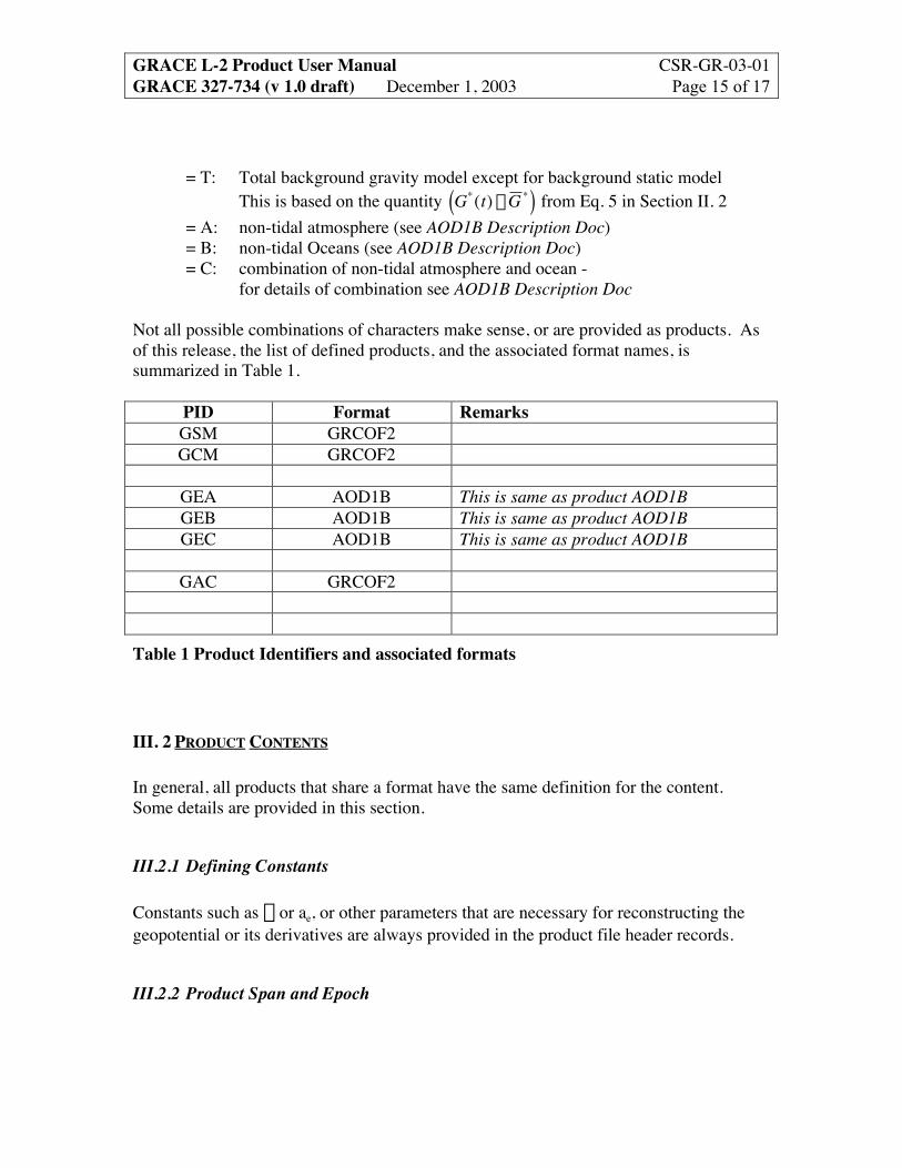
= T: Total background gravity model except for background static modelThis is based on the quantity

†

G*(t) - G *( ) from Eq. 5 in Section II. 2= A: non-tidal atmosphere (see AOD1B Description Doc)= B: non-tidal Oceans (see AOD1B Description Doc)= C: combination of non-tidal atmosphere and ocean -

for details of combination see AOD1B Description Doc

Not all possible combinations of characters make sense, or are provided as products. Asof this release, the list of defined products, and the associated format names, issummarized in Table 1.

PID Format RemarksGSM GRCOF2GCM GRCOF2

GEA AOD1B This is same as product AOD1BGEB AOD1B This is same as product AOD1BGEC AOD1B This is same as product AOD1B

GAC GRCOF2

Table 1 Product Identifiers and associated formats

III. 2 PRODUCT CONTENTS

In general, all products that share a format have the same definition for the content.Some details are provided in this section.

III.2.1 Defining Constants

Constants such as m or ae, or other parameters that are necessary for reconstructing thegeopotential or its derivatives are always provided in the product file header records.

III.2.2 Product Span and Epoch


The product name includes a range of epochs. The start date is the date of the firstobservation or data point used in the processing, and the end date is the date of the lastdata point used. The dates are tracked to at least 1-day discretization, but it is possiblefor the first or the last observation to fall at any time within that day. Finally, it is notassured that all data within the spans in the product identifier were used in the processing.

N.B. Specifically for the GSU or GCU products: Within a fixed data span, identified bythe strings in the product name, it is possible that certain selected geopotential parametersmay be solved as piece-wise constants over sub-intervals of the overall data span. In thiscircumstance, within one product, some coefficients may appear multiple times indifferent records – with a unique span of sub-epochs distinguishing such parameters.

III.2.3 Calibration Coefficients for Uncertainties

For the products GSx or GCx, a scale factor is provided such that calibrated standarddeviation = scale_factor * formal standard deviation.

III.2.4 Companion Documents

Complete specification of the background models and conventions is given in therespective Level-2 Processing Standards Documents. Each data release is associatedwith a corresponding update of this document.

The formats mentioned in Table 1 are contained in the Level-2 Formats Document.


REFERENCES

Heiskanen, W.A. and H. Moritz, Physical Geodesy, W.H. Freeman and Co., 1967.

Torge, W., Geodesy, de Gruyter, New York 1980.

National Research Council, Satellite Gravity and the Geosphere, National AcademyPress, Washington DC, 1997.

Gravity Recovery and Climate...

Documents

Transcript of Gravity Recovery and Climate...