1

EPS 122: Lecture 15 – Gravity and the mantle

Gravitational constraints

Reading: Fowler p206 – 228

EPS 122: Lecture 15 – Gravity and the mantle

Gravity anomalies

Corrected for expected variations due to

• the spheroid

• elevation above the spheroid

• Rock above sea level

Free-air anomaly:

Bouguer anomaly:

Corrected for expected variations due to

• the spheroid

• elevation above the spheroid

2

EPS 122: Lecture 15 – Gravity and the mantle

Isostatic equilibrium

Can we use gravity anomalies to tell if a region is in isostatic equilibrium?

Isostatic equilibrium means no excess mass. Does this mean no gravity anomaly?

Not quite!

Consider the figure:

• Assume isostatic equilibrium

• Bouguer anomaly will be large and negative

• Free-air anomaly: small but positive

WHY?

WHY?

EPS 122: Lecture 15 – Gravity and the mantle

Isostatic equilibrium

Uncompensated

• Large positive Free-air

• Zero Bouguer

Compensated

• Small positive Free-air

• Large negative Bouguer

…away from the edges – why?

3

EPS 122: Lecture 15 – Gravity and the mantle

Australia Topography and

bathymetry

Free-air anomaly Bouguer anomaly

EPS 122: Lecture 15 – Gravity and the mantle

Gravity anomalies

Analytical expressions for simple shapes: Buried sphere

Only the density contrast is important

Gravitational acceleration toward sphere

Gravimeters measure the vertical gravitational acceleration

Mass excess of sphere

Gravity anomaly:

4

EPS 122: Lecture 15 – Gravity and the mantle

Ambiguity An observed gravity anomaly can be explained by a variety of mass distributions at different depths

Observed gravity anomaly

Possible causal structures:

3: Deep sphere

2: Shallower elongated anomaly

1: Even shallower, more elongated structure

Ambiguity in formula for a sphere:

• Trade-off between density and radius

EPS 122: Lecture 15 – Gravity and the mantle

Mid-ocean ridge Gravity observations

Deep model has small density

contrasts

Four density models adequately satisfy the observations

Shallow models have larger density

contrasts

Small positive free-air anomaly,

large negative

bouguer anomaly: close to isostatic

equilibrium

5

EPS 122: Lecture 15 – Gravity and the mantle

Ocean trenches Gravity observations

SEASAT Gravity Map

Largest anomalies are associated with the trenches

• 10 km deep and filled with water rather than rock

• Not compensated as they are being loaded down dip

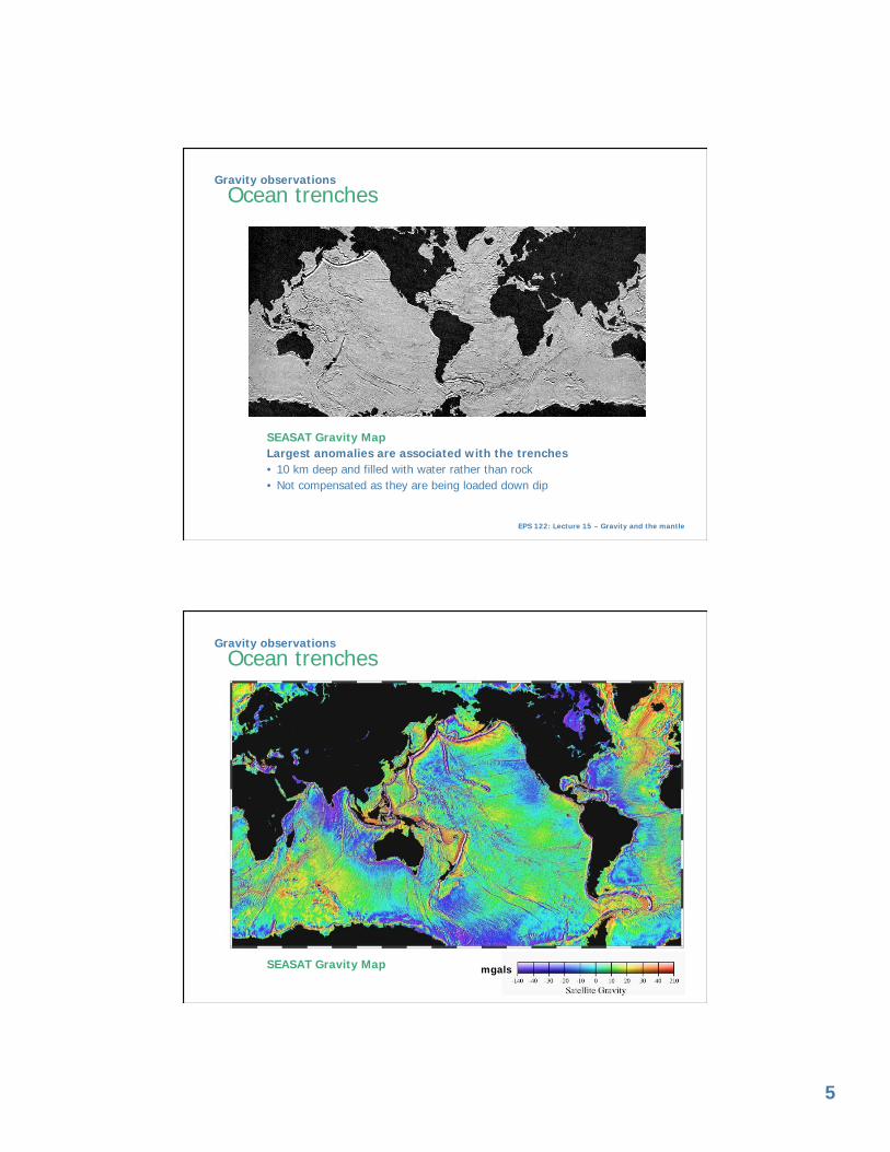
EPS 122: Lecture 15 – Gravity and the mantle

Ocean trenches Gravity observations

SEASAT Gravity Map mgals

6

EPS 122: Lecture 15 – Gravity and the mantle

Subduction profiles Across the Chile Trench

Free air edge effect

Classic low-high pair

• Low over trench

• High on ocean-ward side of the volcanic arc

Density structure – how?

60km thick Andean crust

• Believed to have been thickened from below by intrusive volcanism from slab

Gravity

Topography

Fre

e a

ir

EPS 122: Lecture 15 – Gravity and the mantle

Subduction profiles Across the Chile Trench

Free air edge effect

Gravity

Topography

Fre

e a

ir

1 km water (1000 kg/m3) g = 42 mgal

Estimate the expected gravity anomaly using infinite slab formula:

Universal gravitational constant G=6.67 x 10-11 Nm2/kg2

1 km crust (2700 kg/m3) g = 113 mgal

5 km crust vs. 5 km water: 565 mgal vs. 210 mgal

7

EPS 122: Lecture 15 – Gravity and the mantle

Subduction profiles Across the Japan Trench

Lau Basin

Japan: island arc

Low-high gravity anomaly

Down dip extension

Sea of Japan:

back arc

basin: thin crust

Mantle wedge:

• Low velocity

• High attenuation (low Q)

EPS 122: Lecture 15 – Gravity and the mantle

Geoid height anomalies

The geoid height varies with respect to the spheroid due to lateral density contrasts

At long wavelengths geoid height variations are small

implies that the Earth surface is in broad isostatic equilibrium

The mantle is not strong, it flows in response to loads

in order to achieve isostatic equilibrium

However, small scale topography may not be in isostatic equilibrium

The lithosphere is strong as can support smaller loads

8

EPS 122: Lecture 15 – Gravity and the mantle

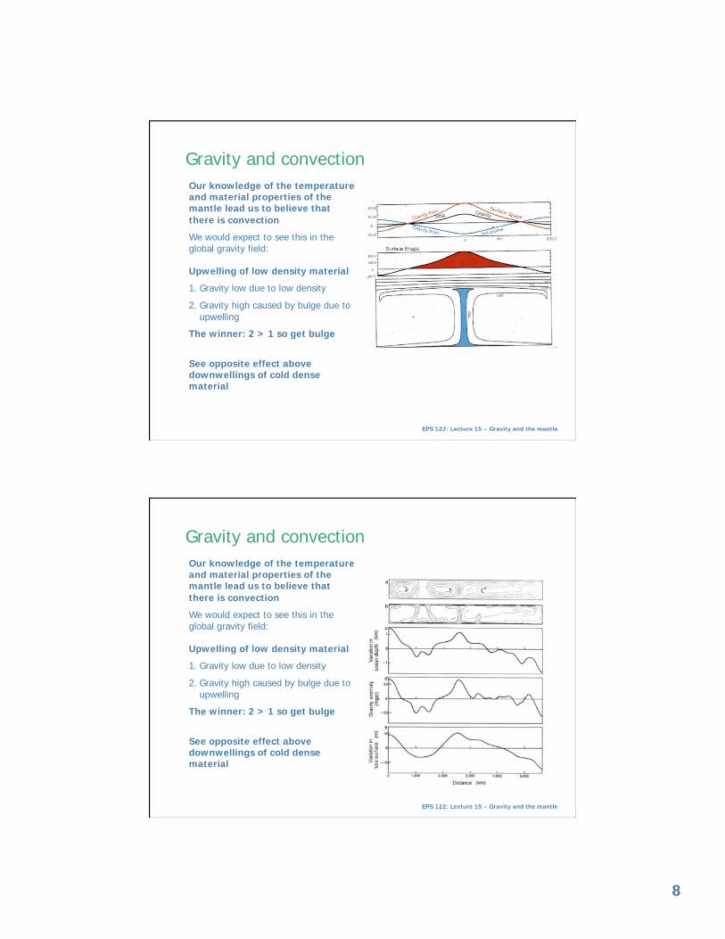
Gravity and convection

Our knowledge of the temperature and material properties of the mantle lead us to believe that

there is convection

We would expect to see this in the global gravity field:

Upwelling of low density material

1. Gravity low due to low density

2. Gravity high caused by bulge due to upwelling

The winner: 2 > 1 so get bulge

See opposite effect above downwellings of cold dense material

EPS 122: Lecture 15 – Gravity and the mantle

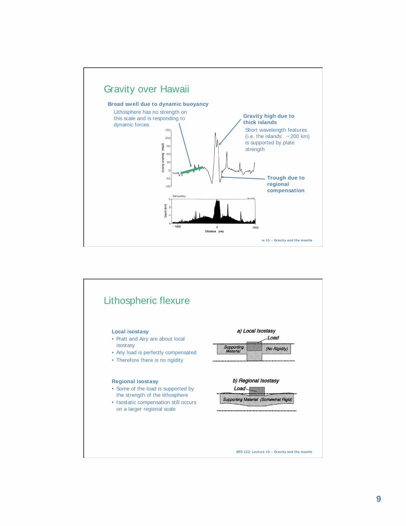
Gravity and convection

Our knowledge of the temperature and material properties of the mantle lead us to believe that

there is convection

We would expect to see this in the global gravity field:

Upwelling of low density material

1. Gravity low due to low density

2. Gravity high caused by bulge due to upwelling

The winner: 2 > 1 so get bulge

See opposite effect above downwellings of cold dense material

9

EPS 122: Lecture 15 – Gravity and the mantle

Gravity over Hawaii

Gravity high due to thick islands

Broad swell due to dynamic buoyancy

Short wavelength features (i.e. the islands: ~200 km) is supported by plate

strength

Lithosphere has no strength on this scale and is responding to dynamic forces

Trough due to regional compensation

EPS 122: Lecture 15 – Gravity and the mantle

Lithospheric flexure

Local isostasy

• Pratt and Airy are about local isostasy

• Any load is perfectly compensated

• Therefore there is no rigidity

Regional isostasy

• Some of the load is supported by the strength of the lithosphere

• Isostatic compensation still occurs

on a larger regional scale

10

EPS 122: Lecture 15 – Gravity and the mantle

The elastic plate

An elastic plate has strength and can be bent to support a load

• The flexural rigidity represents the strength of the plate and is dependent on the elastic thickness

• High flexural rigidity: small depression in response to a load and flexure on a long wavelength

• Low flexural rigidity: large depression and short wavelength response

• Peripheral (or flexural) bulge forms around the load

• Plates with no strength collapse into local isostatic equilibrium

EPS 122: Lecture 15 – Gravity and the mantle

Ocean islands Examples

Hawaii

• Volcanoes load the oceanic plate causing flexure

• By modeling the shape of the flexure we can estimate the elastic thickness of the Pacific plate

• Note: there are two effects here (1) the flexure due to the island load, and (2) the bulge due to mantle upwelling

11

EPS 122: Lecture 15 – Gravity and the mantle

The elastic plate Examples

Subduction zones

• The accretionary wedge loads the end of the plate causing it to bend

• A flexural bulge is often observed adjacent to the trench

Mariana trench

• Topography matched with elastic plate, elastic thickness 28 km

Tonga trench

• Not all subduction zones can be modeled in this way eg the Tonga trench

• Instead this topography needs an elastic plate which deforms plastically once some critical yield stress is applied

EPS 122: Lecture 15 – Gravity and the mantle

Elastic thickness of oceanic plates and their thermal evolution

By modeling the flexure of the plates in response to loads we can estimate the elastic thickness (squares)

This shows an age dependency

• The elastic thickness increases with age and corresponds to the ~450°C isotherm

• Plate strength increases with age

• This is due to the gradual cooling of oceanic lithosphere

Elastic thickness

• of oceans: 10-40 km

• of continents: typically 80-100 km

Note: this is not the lithospheric thickness

12

EPS 122: Lecture 15 – Gravity and the mantle

Isostatic rebound

The rate of deformation after a change in load is dependent on the flexural rigidity of the lithosphere and the

viscosity of the mantle

Need a load large enough which is added or removed quickly enough to observe the viscous response of the mantle

Lake Bonneville, Utah

• dried up 10,000 years ago: 300 m of water load removed

• Center of the lake has risen 65 m

• Viscosity: 1020 to 4x1019 Pa s for 250 to 75 km thick lithosphere

1. Smaller loads: ~100 km diameter

tell us about uppermost mantle viscosity

EPS 122: Lecture 15 – Gravity and the mantle

Isostatic rebound

Scandinavia

• Removal of ice sheet at the end of the last ice age 10,000 years ago:

~2.5 km if ice removed

• Current peak uplift rate is 9 mm/yr

2. Larger loads: ~1000 km diameter

tell us about upper mantle viscosities

A model that satisfies the observed deformation:

• 4x1019 Pa s asthenosphere overlaying

• 1021 Pa s mantle

13

EPS 122: Lecture 15 – Gravity and the mantle

Isostatic rebound

3. Enormous loads: thousands km diameter

tell us about upper and lower mantle viscosities

Wisconsin Ice Sheet

• Extended over Northern US and Canada, up to 3.5 km thick

• Unloading: of continent due to removal of ice sheet at the end of the last ice age 10,000 years ago

• Loading: of the ocean basins due to additional water

Mantle viscosity estimates from isostatic rebound: