Numerical solution for the anisotropic Willmore flow of

graphs

Tomas Oberhuber

Department of Mathematics, Faculty of Nuclear Sciences and Physical Engineering, CzechTechnical University in Prague, Trojanova 13, Praha 2, 120 00, Czech Republic

Abstract

The Willmore flow is well known problem from the differential geometry. It min-imizes the Willmore functional defined as integral of the mean-curvature squareover given manifold. For the graph formulation, we derive modification of theWillmore flow with anisotropic mean curvature. We define the weak solutionand we prove an energy equality. We approximate the solution numerically bythe complementary finite volume method. To show the stability, we re-formulatethe resulting scheme in terms of the finite difference method. By using simpleframework of FDM we show discrete version of the energy equality. The timediscretization is done by the method of lines and the resulting system of ODEsis solved by the Runge-Kutta-Merson solver with adaptive integration step. Wealso show experimental order of convergence as well as results of the numericalexperiments, both for several different anisotropies.

Keywords: Anisotropy, Willmore flow, curvature minimization, gradient flow,Laplace-Beltrami operator, method of lines, complementary finite volumemethod, finite difference method2000 MSC: 35K35, 35K55, 53C44, 65M12, 65M20, 74S20

1. Introduction

This article extends the isotropic Willmore flow defined by T. J. Willmore in[11]. It is a minimizer of the Willmore functional defined as

W (Γ) =

∫Γ

H2dS,

where Γ is given manifold smooth enough so that the mean curvature H can beevaluated almost everywhere on Γ. Prescribing the following normal velocity

V = 4ΓH +H3 − 2HK on Γ (t) ,

Email address: tomas.oberhuber@fjfi.cvut.cz ()URL: http://geraldine.fjfi.cvut.cz/~oberhuber ()

Preprint submitted to ??? November 4, 2018

arX

iv:1

111.

3043

v1 [

mat

h.N

A]

13

Nov

201

1

we generate class of manifolds Γ (t) so that Γ (t) minimizes the Willmore func-tional as t goes to infinity. One recognizes several formulation of the Willmoredepending of the form in which Γ (t) is expressed - the graph formulation [4, 8, 12],the level-set formulation [5, 1] or the parametric formulation [7, 1]. Also approx-imation by the phase-field model exists [6]. In this article we will study only thegraph formulation. Applications of the Willmore flow can be found in biology [3]or in image processing in image inpainting [2]. Especially in the later one, theanisotropic model can be useful.

2. Problem formulation

We assume having a manifold Γ0 described as a graph of function u0 of twovariables:

Γ0 =

[x, u0 (x)] | x ∈ Ω ⊂ R2, (1)

where Ω ≡ (0, L1)× (0, L2) is an open rectangle and we will denote ∂Ω its bound-ary. We assume having convex function γ : Rn+1\0 → R

+0 , γ = γ(p1, · · · pn,−1)

which is positive 1-homogeneous i.e. γ (λp) = |λ| γ (p). We will call γ surfaceenergy density and denote

∇pγ =(∂p1γ, · · · , ∂pnγ

),

where ∂piγ stands for partial derivatives of γ w.r.t. variable pi. We defineanisotropic mean curvature of a manifold Γ0 smooth enough induced by energydensity function γ as

Hγ (u0) = ∇ · (∇pγ (∇u0,−1)) . (2)

and the anisotropic Willmore functional as

Wγ (u0) =1

2

∫Ω

H2γ (u0)Q (u0) dx, (3)

for Q (u) =√

1 + |∇u|2. We aim to find a function u∗ minimizing (3). The

Euler-Lagrange equation for this functional takes the following form

∇ ·(Eγ (u∗)∇wγ (u∗)− 1

2

w2γ (u∗)

Q3 (u∗)∇u∗

)= 0, (4)

where we denoted

wγ (u) := Q (u)Hγ (u) ,

Eγ (u) := ∂pi∂pjγ (∇u,−1) = (∇p ⊗∇p) γ (∇u,−1) .

2

In the rest of the text we will not emphasize explicitly the dependence ofQ,Hγ, wγand Eγ on u. Multiplying (4) by the test function ϕ ∈ C∞ (Ω) and integratingover Ω we get

0 =

∫Ω

∇ ·(Eγ∇wγ −

1

2

w2γ

Q3∇u)ϕdx =

−∫∂Ω

Eγ∇wγ · νϕ+1

2

w2γ

Q3∇u · νϕdS +

∫Ω

∇ · (Eγ∇wγ)ϕ−1

2∇ ·(w2γ

Q3∇u)ϕdx.

The boundary integral over ∂Ω vanishes if we set

∂νu = 0 on ∂Ω, (5)

Eγ∇wγ · ν = 0 on ∂Ω. (6)

These relations define the Neumann boundary conditions. The Dirichlet bound-ary conditions

u = g1 on ∂Ω, (7)

wγ = g2 on ∂Ω, (8)

may be obtained in the same way but taking ϕ ∈ C∞0 (Ω). In practice, the L2-gradient flow of (3) is solve rather than (4) – see [4, 5]. The following definitioninvolves parabolic partial differential equation with unknown function u which isnow also dependent on artificial time parameter t i.e. u = u (t,x). In the samesense as in (1), a moving manifold Γ (t) is obtained.

Definition 2.1. Let Ω be a domain in R2. The anisotropic Willmore flowof graphs with the Dirichlet boundary conditions and the initial conditionu0 is a fourth order parabolic problem given by

∂tu = −Q∇ ·(Eγ∇wγ −

1

2

w2γ

Q3∇u)

on (0, T )× Ω, (9)

wγ = QHγ on (0, T )× Ω, (10)

u |t=0 = u0 on Ω, (11)

u = g1, wγ = g2 on ∂Ω. (12)

The anisotropic Willmore flow of graphs with the Neumann boundaryconditions and the initial condition u0 is a fourth order parabolic problem givenby (9)–(11) and

∂νu = 0, Eγ∇wγ · ν = 0 on ∂Ω. (13)

We also define the weak formulation:

3

Definition 2.2. Let Ω be a domain in R2. The weak solution of anisotropicWillmore flow of graphs with the Dirichlet boundary conditions

u = g1 on ∂Ω,

wγ = g2 on ∂Ω,

is a couple u,wγ : (0, T ) → H10 (Ω) which for each test function ϕ, ξ ∈ H1

0 (Ω)and a.e in (0, T ) satisfies,∫

Ω

utQϕdx =

∫Ω

(Eγ∇wγ) · ∇ϕ−1

2

w2γ

Q3∇u · ∇ϕdx a.e. in (0, T ) (14)∫

Ω

wγQξdx = −

∫Ω

∇pγ · ∇ξdx. (15)

with the initial conditionu |t=0= u0. (16)

The weak solution of anisotropic Willmore flow of graphs with homo-geneous Neumann boundary conditions

∂νu = 0 on ∂Ω,

Eγ∇w · ν = 0 on ∂Ω,

is a couple u,w : (0, T )→ H1 (Ω) which for each test function ϕ, ξ ∈ H1 (Ω) anda.e. in (0, T ) satisfies (14)-(15) and the initial condition (16).

For the proof of the numerical stability we will need the following theorem:

Theorem 2.3. For the solution u,wγ of (14)-(16) with the zero Dirichlet bound-ary conditions the following energy equality holds:∫

Ω

(∂tu)2

Qdx +

1

2

d

dt

∫Ω

H2γQdx = 0. (17)

Proof. We differentiate (15) with respect to t∫Ω

∂twγξ

Qdx−

∫Ω

wγξ∂tQ

Q2dx +

∫Ω

Eγ∇∂tu · ∇ξ = 0 for all ξ ∈ H10 (Ω) (18)

which follows from

d

dt∇pγ (∇u,−1) · ∇ξ =

d

dt

n∑i=1

∂piγ (∇u,−1) ∂piξ

=n∑

i,j=1

∂pi∂pjγ (∇u,−1) ∂t∂xju∂piξ

= Eγ∇∂tu · ∇ξ.

4

Substituting ϕ = ∂tu in (14) and ξ = wγ in (18) we have∫Ω

(∂tu)2

Qdx−

∫Ω

(Eγ∇wγ) · ∇∂tudx +

∫Ω

1

2

w2γ

Q3∇u · ∇∂tudx = 0, (19)∫

Ω

∂twγwγQ

dx−∫

Ω

w2γ∂tQ

Q2dx +

∫Ω

(Eγ∇∂tu) · ∇wγ = 0 (20)

The sum of (19) and (20) gives∫Ω

(∂tu)2

Q+∂twγwγQ

− w2γ∂tQ

Q2+

1

2

w2γ

Q3∇u · ∇∂tudx = 0.

Since ∇∂tu · ∇u = ∂tQQ, (1) turns to∫Ω

(∂tu)2

Q+∂twγwγQ

− 1

2

w2γ∂tQ

Q2dx = 0,

which is indeed what we wanted to show because

1

2

d

dtH2γQ =

1

2

d

dt

w2γ

Q=∂twγwγQ

− 1

2

w2γ∂tQ

Q2.

We will demonstrate the anisotropic Willmore flow of graphs on the following(an)isotropies:

γiso (p) :=

√1 + |p|2, (21)

γG (p,−1) :=√

1 + pTGp, (22)

γabs (P) :=3∑i=1

√√√√P 2i + εabs

3∑j=1

P 2j , (23)

where G is symmetric positive definite matrix G ∈ R2,2 and we use notationP = (p,−1). In fact, γiso represents the isotropic problem. The Wulf shapes Wof given anisotropies defined by

W =⋂|q|=1

x ∈ Rn | (x,q) ≤ γ (q) , (24)

are depicted on the Figure 1. Simple calculations show that

Hγiso = ∇ ·

∇u√1 + |∇u|2

, Eγiso =1

Q

(I− ∇u

Q⊗ ∇u

Q

), (25)

HγG = ∇ ·(G∇uγG

), EγG =

1

γG

(G− G∇u

γG⊗ G∇u

γG

). (26)

5

Figure 1: The Wulf shapes of γiso, γG and γabs from left to right.

It is difficult to express Hγabs and Eγabs in some compact form and so we onlyshow partial derivatives of γabs with respect to pi and pj for i, j = 1, 2.

γabs,pi =3∑j=1

εabspi√P 2j + εabs

∑3k=1 P

2k

+pi√

p2i + εabs

∑3j=1 P

2j

for i = 1, 2,

γabs,pipi =3∑j=1

εabs√P 2j + εabs

∑3k=1 P

2k

− ε2absp2i(

P 2j + εabs

∑3k=1 P

2k

) 32

+

1√p2i + εabs

∑3j=1 P

2j

− p2i(

p2i + εabs

∑3j=1 P

2j

) 32

for i = 1, 2,

γabs,pipj = −3∑

k=1

ε2abspipj(P 2k + εabs

∑3l=1 P

2l

) 32

−2∑

k=1

εabspipj(P 2k + εabs

∑3l=1 P

2l

) 32

.

3. Space discretization

3.1. The complementary-finite volume method

In [9] we applied the complementary-finite volume method for the space dis-cretization of the anisotropic surface-diffusion flow. In the same manner we dis-cretize even the problem from the Definition 2.1. Let h1, h2 be space steps suchthat h1 = L1

N1and h2 = L2

N2for some N1, N2 ∈ N+. We define a numerical grid,

its closure and its boundary as

ωh = (ih1, jh2) | i = 1 · · ·N1 − 1, j = 1 · · ·N2 − 1 , (27)

ωh = (ih1, jh2) | i = 0 · · ·N1, j = 0 · · ·N2 , (28)

∂ωh = ωh \ ωh. (29)

For u ∈ C(Ω)

we define its piecewise constant approximation on ω as a gridfunction uh defined as uh (ih1, jh2) := uhij := u (ih1, jh2). We also define a dual

6

(0, 0) (N1, 0)

(0, N2) (N1, N2)

vij

vi+1,jvi−1,j

vi,j+1

vi,j−1

νij,i+1j = (1, 0)νij,i−1j = (−1, 0)

νij,ij+1 = (0, 1)

νij,ij−1 = (0,−1)

a) b)

Figure 2: (a) Dual mesh for the complementary finite volumes method - dots denote ωh (27),circles denote ∂ωh (29) and solid lines stand for Vh (30). (b) Notation for νij,ij .

mesh Vh as (see the Figure 2 a))

Vh ≡vij =

[(i− 1

2

)h1,

(i+

1

2

)h1

]×[(j − 1

2

)h2,

(j +

1

2

)h2

]|

i = 1 · · ·N1 − 1, j = 1 · · ·N2 − 1

. (30)

For 0 < i < N1, 0 < j < N2, i and j fixed, consider a finite volume vij of thedual mesh Vh, denote its interior as Ωij, its boundary as Γij and let µ (Ωij) be thevolume of Ωij. We also denote all the neighboring volumes of the volume vij asNij. For all finite volumes vij of the dual mesh Vh, the boundary Γij consists offour linear segments. We denote them as Γij,ij. It means that Γij,ij is a boundaryof the finite volume vij between nodes (i, j) and (i, j). By lij,ij we denote thelength of this part of Γij. We approximate the partial derivatives of u on theboundary of the finite volume vij as (here ∂hx1

resp. ∂hx2stands for the finite

difference w.r.t. x1 resp. x2):

∂hx1uhij,i+1j =

uhi+1j − uhijh1

, ∂hx1uhij,i−1j =

uhij − uhi−1j

h1

,

∂hx2uhij,ij+1 =

uhij+1 − uhijh2

, ∂hx2uhij,ij−1 =

uhij − uhij−1

h2

,

and

∂hx2uhij,i+1j =

uhij,i+1j+1 − uhij,i+1j−1

h2

, ∂hx2uhij,i−1j =

uhij,i−1j+1 − uhij,i−1j−1

h2

,

∂hx1uhij,ij+1 =

uhij,i+1j+1 − uhij,i−1j+1

h1

, ∂hx1uij,ij−1 =

uij,i+1j−1 − uij,i−1j−1

h1

,

7

where we denote

uhij,i+1j+1 =1

4

(uhij + uhi+1j + uhij+1 + uhi+1j+1

)uhij,i+1j−1 =

1

4

(uhij + uhi+1j + uhij−1 + uhi+1j−1

)uhij,i−1j+1 =

1

4

(uhij + uhi−1j + uhij+1 + uhi−1j+1

)uhij,i−1j−1 =

1

4

(uhij + uhi−1j + uhij−1 + uhi−1j−1

).

The quantity Q on the boundary of Γij is approximated as

Qhij,i+1j =

√1 +

(∂hx1

uhij,i+1j

)2+(∂hx2

uhij,i+1j

)2,

Qhij,ij+1 =

√1 +

(∂hx1

uhij,ij+1

)2+(∂hx2

uhij,ij+1

)2,

Qhij,i−1j =

√1 +

(∂hx1

uhij,i−1j

)2+(∂hx2

uhij,i−1j

)2,

Qhij,ij−1 =

√1 +

(∂hx1

uhij,ij−1

)2+(∂hx2

uhij,ij−1

)2,

and Q inside the finite volume vij as

Qhij =

1

4

(Qhij,i+1j +Qh

ij,ij+1 +Qhij,i−1j +Qh

ij,ij−1

).

Integrating (2) over a finite volume Ωij and applying the Stokes formula we obtain∫Ωij

Hγdx =

∫Ωij

∇ · (∇pγ) dx =

∫Γij

∇pγ · νdS. (31)

where ν denotes the outer unit normal vector to the finite volume boundary Γij.We approximate the term on the left as∫

Ωij

Hγdx ≈ µ (Ωij)Hhγ,ij (32)

and the term on the right as∫Γij

∇pγ · νdS =∑

vij∈Nij

∫Γij,ij

∇pγ · νdS (33)

For the inner finite volume vij ∈ Vh, there are four different neighbors vij ∈ Nij(see the Figure 30). All the boundaries Γij,ij are linear segments and so ν = νij,ijis constant there. Moreover we assume that ∇pγ is constant along Γij,ij too. Itgives ∑

vij∈Nij

∫Γij,ij

∇pγ · νdS ≈∑

vij∈Nijlij,ij∇pγij,ij · νij,ij (34)

8

where

∇pγij,ij =(∂p1γij,ij, ∂p2γij,ij

)T=(∂p1γ

(∇uhij,ij,−1

), ∂p2γ

(∇uhij,ij,−1

))T. (35)

Putting (32) and (34) together we get

µ (Ω)Hhγ,ij =

∑vij∈Nij

lij,ij∇pγij,ijνij,ijdS, (36)

For the regular dual mesh (30) we have

Hhγ,ij =

1

h1h2

(h2∇pγij,i+1j · (1, 0)T + h1∇pγij,ij+1 · (0, 1)T

+ h2∇pγij,i−1j · (−1, 0)T + h1∇pγij,ij−1 · (0,−1)T)

=

(∂p1γij,i+1j − ∂p1γij,i−1,j

h1

+∂p2γij,ij+1 − ∂p2γij,ij−1

h2

), (37)

and the approximation of wγ = QHγ on the finite volume Ωij is

whγ,ij = QhijH

hγ,ij. (38)

We set

whγ,ij,i+1j =1

2

(whγ,ij + whγ,i+1j

), whγ,ij,ij+1 =

1

2

(whγ,ij + whγ,ij+1

), (39)

whγ,ij,i−1j =1

2

(whγ,ij + whγ,i−1j

), whγ,ij,ij−1 =

1

2

(whγ,ij + whγ,ij−1

). (40)

Integrating (9) over Ωij and applying the Stokes theorem we get∫Ωij

1

Q∂tudx = −

∫Γij

Eγ∇wγν −1

2

w2γ

Q3∂νudS (41)

where ν is the unit outer normal of the boundary Γij. The left hand side isapproximated as follows:∫

Ωij

1

Q∂tudx ≈ µ (Ωij)

Qhij

d

dtuhij = h1h2

1

Qhij

d

dtuhij, (42)

where we assume that uhij and Qhij are constant on the element vij. For the integral

on the right hand side of (41) we have

−∫

Γij

Eγ∇wγν −1

2

w2γ

Q3∂νudS ≈

−∑

vij∈Nijlij,ij

Ehγ,ij,ij∇whγ,ij,ijνij,ij −1

2

(whγ,ij,ij

)2

(Qhij,ij

)3 ∇ij,ijuhijνij,ij

. (43)

9

with the usual notation. Putting (42) and (43) together gives

d

dtuhij = − Qh

ij

µ (Ωij)

∑ij∈Nij

lij,ij

Ehγ,ij,ij∇whγ,ij,ijνij,ij −1

2

(whγ,ij,ij

)2

(Qhij,ij

)3 ∇ijijuhijνij,ij

.

In the terms of the regular dual mesh (30) we get

d

dtuhij = − Qh

ij

h1h2

[h2

(Ehγ,ij,i+1j∇whγ,ij,i+1j (1, 0)T − 1

2

(whγ,ij,i+1j

)2(Qhij,i+1j

)3 ∇uhij,i+1j (1, 0)T)

+ h1

(Ehγ,ij,ij+1∇whγ,ij,ij+1 (0, 1)T − 1

2

(whγ,ij,ij+1

)2(Qhij,ij+1

)3 ∇uhij,ij+1 (0, 1)T)

+ h2

(Ehγ,ij,i−1j∇whγ,ij,i−1j (−1, 0)T − 1

2

(whγ,ij,i−1j

)2(Qhij,i−1j

)3 ∇uhij,i−1j (−1, 0)T)

+ h1

(Ehγ,ij,ij−1∇whγ,ij,ij−1 (0,−1)T − 1

2

(whγ,ij,ij−1

)2(Qhij,ij−1

)3 ∇uhij,ij−1 (0,−1)T)]

.

where for

Ehγ,ij,ij =

(Ehγ,11,ij,ij E

hγ,12,ij,ij

Ehγ,21,ij,ij E

hγ,22,ij,ij

), (44)

we have

Ehγ,ij,i+1j = ∂p1∂p1γ(∇uhij,i+1j,−1

), Ehγ,ij,ij+1 = ∂p1∂p2γ

(∇uhij,ij+1,−1

),

Ehγ,ij,i−1j = ∂p1∂p1γ(∇uhij,i−1j,−1

), Ehγ,ij,ij−1 = ∂p1∂p2γ

(∇uhij,ij−1,−1

).

The Neumann boundary condition ∂νu = 0 on ∂Ω takes the following discreteform

if i = 1 then ν = (−1, 0) ⇒ 1

h1

(uh1,j − uh0,j

)= 0, (45)

if i = N1 − 1 then ν = (1, 0) ⇒ 1

h1

(uhN1,j

− uhN1−1,j

)= 0, (46)

if j = 1 then ν = (0,−1) ⇒ 1

h2

(uhi,1 − uhi,0

)= 0, (47)

if j = N2 − 1 then ν = (0, 1) ⇒ 1

h2

(uhi,N2

− uhi,N2−1

)= 0 (48)

10

and from (13) we get

if i = 1 then ν = (−1, 0) ⇒ Eγ,11,1j,0j∂x1whγ,1j,0j +Eγ,12,1j,0j∂x2w

hγ,1j,0j = 0,

(49)

if i = N1 − 1 then ν = (1, 0) ⇒ Eγ,11,N1−1j,N1j∂x1whγ,N1−1j,N1j

+

Eγ,12,N1−1j,N1j∂x2whγ,N1−1j,N1j

= 0, (50)

if j = 1 then ν = (0,−1) ⇒ Eγ,21,i1,i0∂x1whγ,i1,i0 +Eγ,22,i1,i0∂x2w

hγ,i1,i0 = 0,

(51)

if j = N2 − 1 then ν = (0, 1) ⇒ Eγ,21,iN2−1,iN2∂x1whγ,iN2−1.iN2

+

Eγ,22,iN2−1,iN2∂x2whγ,iN2−1,N2

= 0. (52)

3.2. The finite difference method

We will prove the discrete version of the Theorem 2.3 in very similar manneras in [8]. For this purpose we need to re-formulate the complementary finitevolume scheme by the finite difference method. We complete the numerical gridwith virtual nodes representing the finite volumes edges and we denote the newgrid by $h. We index the nodes of $h by indices i ± 1

2and j ± 1

2. We define

uhi± 1

2j± 1

2

= 12

(uhi±1,j±1 + uhij

)and denote by the uppercase a grid function with

doubled indices i.e.Uhkl = uhk

2l2

for k, l ∈ 0 · · · 2N. (53)

We introduce the finite differences as follows:

Uhf.,kl = 2

Uhk+1,l − Uh

kl

h, Uh

b.,kl = 2Uhkl − Uh

k−1,l

h,

Uh.f,kl = 2

Uhk,l+1 − Uh

kl

h, Uh

.b,kl = 2Uhkl − Uh

k,l−1

h,

Uhc.,kl =

1

2

(Uhf.,kl + Uh

b.,kl

), Uh

.c,kl =1

2

(Uh.f,kl + Uh

.b,kl

)To approximate the gradient of u we define

∇huhij =(Uhc.,2i,2j, U

h.c,2i,2j

)for i, j ∈ 1 · · ·N − 1

Note that since we define ∇huhij in terms of Uhkl we can also write ∇huh

i± 12,j± 1

2

for

i, j = 1 · · ·N − 1. The terms in (9)-(10) are approximated as follows

Qhi± 1

2,j± 1

2=

√1 +

∣∣∣∇huhi± 1

2,j± 1

2

∣∣∣2 , Qhij =

1

4

∑ζ,η∈−1,1)|ζ|+|η|=1

Qhi+ ζ

2,j+ η

2

,

Ehγ,ij = Eγ

(uhij)

, Hhγ,ij = Hγ

(uhij)

11

and the scheme has a form

duh

dt= −Qh

ij∇h ·(Ehγ,ij∇hwhγ,ij −

1

2

(whγ,ij

)2(Qhij

)3 ∇huhij

), (54)

whγ,ij = QhijH

hγ,ij (55)

Approximation of the Dirichlet boundary conditions is straightforward and theNeumann boundary conditions are handled as in (45)–(52). In what follows wedefine several discrete scalar products and we prove the discrete version of theGreen formula. Assume having f, g : ωh → R, f : ωh → R

2 and the relatedfunctions F,G : $h → R, F : $h → R

2 given by (53) we define

[F,G]PQpq =h1h2

4

P,Q∑k=p,l=q

FklGkl, (f, g)h = (F,G)h = [F,G]2N−1,2N−111 ,

(F,Gc.)c = [F,Gf.]2N−1,2N−10,1 + [F,Gb.]

2N,2N−11,1 ,

(F,G.c)c = [F,G.f ]2N−1,2N−11,0 + [F,G.b]

2N−1,2N1,1 ,(

F ,∇hG)c

=(F 1, Gc.

)c

+(F 2, G.c

)c

For the purpose of analysis, we will need the following grid version of the Greenformula

Lemma 3.1. Let uh, vh : ωh → R and Uh, V h : $h → R related to u, v by (53).Then the Green formula is valid:(

∇huh, vh)h

= −(uh,∇hvh

)c

+h1

2

(2N−1∑l=1

[(Uh

2N−1,l + Uh2N,l

)V h

2N,l −(Uh

0l + Uh1l

)V h

0l

])

+h2

2

(2N−1∑k=1

[(Uhk,2N−1 + Uh

k,2N

)V hk,2N −

(Uhk0 + Uh

k1

)V hk0

])

Proof. It is easy to see that for fixed k, l = 0, · · · 2N the following relationsholds. [

Uhb., V

h]2N−1,l

1,l= −

[U, V h

f.

]2N−1,l

0,l+h1

2

(Uh

2N−1,lVh

2N,l − Uh0lV

h0l

), (56)[

Uhf., V

h]2N−1,l

1,l= −

[U, V h

b.

]2N,l1,l

+h1

2

(Uh

2N,lVh

2N,l − Uh1lV

h0l

), (57)[

Uh.b, V

h]k,2N−1

k,1= −

[U, V h

.f

]k,2N−1

k,0+h2

2

(Uhk,2N−1V

hk,2N − Uh

k0Vhk0

)(58)[

Uh.f , V

h]k,2N−1

k,1= −

[U, V h

.b

]k,2Nk,1

+h2

2

(Uhk,2NV

hk,2N − Uh

k1Vhk0

)(59)

12

Putting together (56) with (57) resp. (58) with (59) and summing over l =1, · · · 2N − 1 resp. over k = 1, · · · 2N − 1 we obtain

(Uhc., V

h)h

= −(U, V h

c.

)c

+h1

2

2N−1∑l=1

[(Uh

2N−1,l + Uh2N,l

)V h

2N,l −(Uh

0l + Uh1l

)V h

0l

],

(Uh.c, V

h)h

= −(U, V h

.c

)c

+h2

2

2N−1∑k=1

[(Uhk,2N−1 + Uh

k,2N

)V hk,2N −

(Uhk0 + Uh

k1

)V hk0

],

which gives(∇hU, V h

)h

= −(U,∇hV

)c

+h1

2

(2N−1∑l=1

[(Uh

2N−1,l + Uh2N,l

)V h

2N,l −(Uh

0l + Uh1l

)V h

0l

])

+h2

2

(2N−1∑k=1

[(Uhk,2N−1 + Uh

k,2N

)V hk,2N −

(Uhk0 + Uh

k1

)V hk0

])

The following form of the previous Lemma 3.1 will be more convenient for us:

Lemma 3.2. Let ph, uh, vh : ωh → R and v |∂ω= 0. Then(∇h ·

(ph∇huh

), vh)h

= −(ph∇huh,∇hvh

)c. (60)

Theorem 3.3. For solution of (54)–(55) such that uh |∂ωh= 0 and whγ = 0 |∂ωhthe following energy equality holds((

uht)2,

1

Qh

)h

+d

dt

((Hhγ

)2, Qh

)h

= 0.

Proof. We start with the equation for whγ,ij (55), divide by Qhij, multiply by ξij

vanishing on ∂ωh and sum over ω.(whγQh

, ξ

)h

=(∇h ·

(γp(∇huh,−1

)), ξ)h.

The Green theorem (60) gives(whγQh

, ξ

)h

= −(∇hξ,∇p

(∇huh,−1

)). (61)

13

Taking the right hand side of (54), multiplying by a test function ϕ vanishing at∂ωh and applying the Green theorem (60) we obtain(−∇h ·

(2Eh∇hwhγ −

(whγ)2

(Qh)3∇huh

), ϕ

)h

=

(2Eh∇hwhγ −

(whγ)2

(Qh)3∇huh,∇hϕ

)c

.

(62)

Differentiating (61) with respect to t we obtain

d

dt

(whγQh

, ξ

)h

+d

dt

(∇piγ

(∇huh,−1

),∇hξ

)c

=

d

dt

(whγQh

, ξ

)h

+((∇p ⊗∇p) γ

(∇huh,−1

)∇huht ,∇hξ

)c

=

(whγ,tQh

, ξ

)h

−(Qht · whγ

(Qh)2 , ξ

)h

+(Eh∇huht ,∇hξ

)c

= 0.

After substituting ξ = whγ we obtain(whγ,tQh

, whγ

)h

−(

Qht

(Qh)2 ,(whγ)2)h

+(Eh∇huht ,∇hwhγ

)c

= 0, (63)

and a substitution ϕ = uht in (62) gives((uht)2,

1

Qh

)h

−(

2Eh∇hwhγ −(whγ)2

(Qh)3∇huh,∇huht

)c

= 0. (64)

Substituting (63) to (64) (term Eh∇hwh) we have((uht)2,

1

Qh

)h

+

(whγ,tQh

, whγ

)h

−(

Qht

(Qh)2 ,(whγ)2)h

+((whγ)2

(Qh)3 ,∇huh · ∇huht

)c

= 0. (65)

We remind that ∇huh · ∇huht = Qh ·Qht which gives((

uht)2,

1

Qh

)h

+

(whγ,tQh

, whγ

)h

−(

Qht

(Qh)2 ,(whγ)2)h

+

((whγ)2

(Qh)2 , Qht

)c

= 0.

(66)

14

It is equivalent to((uht)2,

1

Qh

)h

+

(whγ,t

(Qh)2 , whγ

)h

−(

Qht

(Qh)2 ,(whγ)2)h

+ Sh = 0, (67)

for

Sh =h2

1

4

2N−1∑i=1

(whγ,i,2NQhi,2N

)2

·Qht,i,2N +

(whγ,i0Qhi0

)2

·Qht,i0

+

h22

4

2N−1∑j=1

(whγ,2NjQh

2Nj

)2

·Qht,2Nj +

(whγ,0jQh

0j

)2

·Qht,0j

.Finally from (67) we have((

uht)2,

1

Qh

)h

+d

dt

((Hhγ

)2, Qh

)h

+ Sh = 0.

The term Sh is vanishing on ∂ω because of the zero Dirichlet boundary conditions.

4. Time discretization

The semi-discrete problem (44) is discretize in time by the method of linesin the same way as in [10]. Here, the resulting system of ODEs is solved by theRunge-Kutta-Merson solver with adaptive integration time step implemented inCUDA to run on GPU.

5. Experimental order of convergence

To our best knowledge, there is not known any analytical solution for theWillmore flow of graphs even in the isotropic case. To be able to measure the ex-perimental order of convergence we will solve a modified problem with additionalforcing term F having the following form:

∂tu = −Q∇ ·(Eγ∇wγ −

1

2

w2γ

Q3∇u)

+ F (u) on (0, T )× Ω, (68)

wγ = QHγ on (0, T )× Ω, (69)

u |t=0 = u0 on Ω, (70)

u = g, wγ = 0 on ∂Ω. (71)

Having a function ζ (x, t), we set

FW (ζ) = Q (ζ)∇ ·(

1

Q (ζ)P (ζ)∇wγ (ζ)− 1

2

w2γ (ζ)

Q3 (ζ)∇ζ)

+ ∂tζ on Ω× [0, T ] ,

wγ (ζ) = Q (ζ)Hγ (ζ) on Ω× [0, T ] .

15

As an analytical solution ζ(x, t) of (68)–(71) we chose the following function

ζ (x, y, t) := cos (πt)1

r2n(xn − rn) (yn − rn) exp

(−σ(x2 + y2

))on Ω× [0, T ],

(72)for Ω ≡ [−r, r]2. For given T , we evaluate the errors in the norms of the spacesL1 (Ω; [0, T ]), L2 (Ω; [0, T ]) and L∞ (Ω; [0, T ]) resp. their approximations

∥∥uh − Ph (ζ)∥∥h,τL1(ωh;[0,T ])

:=

N1,N2,M∑i,j,k=0

τ∣∣uhij (kτ)− ζ (−r + ih,−r + jh, kτ)

∣∣h2, (73)

∥∥uh − Ph (ζ)∥∥h,τL2(ωh;[0,T ])

:=

(N1,N2,M∑i,j,k=0

τ(uhij (kτ)− ζ (−r + ih,−r + jh, kτ)

)2h2

) 12

,

(74)∥∥uh − Ph (ζ)∥∥h,τL∞(ωh;[0,T ])

:= maxi=0,··· ,N1j=0,··· ,N2k=0,··· ,M

∣∣uhij (kτ)− ζ (−r + ih,−r + jh, kτ)∣∣ , (75)

for τ = T/M . We would like to emphasize that τ does not correspond with thetime step of the solver. The experimental order of convergence is evaluated asfollows - for two approximations uh1 and uh2 obtained by the discretization withthe space steps h1 and h2 we compute the approximation errors Errh1 and Errh2

in one norm of (73)–(75) and then we set

EOC (Errh1 , Errh2) :=log (Errh1/Errh2)

log (h1/h2). (76)

The results are presented in the Tables 1–8. The solution of (68)–(71) was ap-proximated on the domain Ω ≡ [−4, 4]2 and the time interval [0, 0.1]. The Tables1 – 2 show EOC for u and w with the isotropic setting. Both unknown functionsare approximated with the second order. The Tables 3 – 4 show anisotropy (22)where

G =

(2 00 1

). (77)

Even in this case we obtained EOC equals to 2. As we can see in the Tables 5 –6, if we set

G =

(2 11 1

), (78)

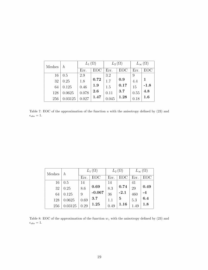
mixed partial derivatives are involved and EOC drops drops to 1 for both u andwγ. The last test is with the anisotropy given by (23) and we set εabs = 0.1.Results are presented in the Tables 7 and 8. The non-linearity is much strongerhere and it is not clear whether EOC is 1 or 2 from the Tables 7 and 8. It wouldrequire computation on finer meshes which we were not able to do because ofvery long time needed for such simulation.

16

Meshes hL1 (Ω) L2 (Ω) L∞ (Ω)

Err. EOC Err. EOC Err. EOC16 0.5 0.09 0.2 1.05

32 0.25 4.37 · 10−3 4.5 4.39 · 10−3 5.52 2.82 · 10−2 5.21

64 0.125 9.96 · 10−4 2.13 7.55 · 10−4 2.54 1.68 · 10−3 4.06

128 0.0625 2.49 · 10−4 1.99 1.89 · 10−4 1.99 4.22 · 10−4 1.99

256 0.03125 6.25 · 10−5 1.99 4.74 · 10−5 1.00 1.05 · 10−4 1.99

Table 1: EOC of the approximation of the function u with the anisotropy defined by (21).

Meshes hL1 (Ω) L2 (Ω) L∞ (Ω)

Err. EOC Err. EOC Err. EOC16 0.5 0.48 0.83 3.65

32 0.25 3.19 · 10−2 3.92 4.89 · 10−2 4.09 0.53 2.77

64 0.125 7.02 · 10−3 2.18 7.79 · 10−3 2.65 8.81 · 10−2 2.59

128 0.0625 1.76 · 10−3 1.99 1.91 · 10−3 2.02 2.1 · 10−2 2.06

256 0.03125 4.40 · 10−4 2 4.75 · 10−4 2 5.2 · 10−3 2.01

Table 2: EOC of the approximation of the function wγ with the anisotropy defined by (21).

Meshes hL1 (Ω) L2 (Ω) L∞ (Ω)

Err. EOC Err. EOC Err. EOC16 0.5 0.7 1.2 5.5

32 0.25 0.53 0.4 0.93 0.37 4.9 0.17

64 0.125 0.085 2.6 0.24 2 1.5 1.8

128 0.0625 0.0059 3.8 0.013 4.2 0.089 4

256 0.03125 0.0015 2 0.0035 1.9 0.024 1.9

Table 3: EOC of the approximation of the function u with the anisotropy defined by (22) and(77).

17

Meshes hL1 (Ω) L2 (Ω) L∞ (Ω)

Err. EOC Err. EOC Err. EOC16 0.5 3.5 7.3 41

32 0.25 3.2 0.15 7.3 0 44 -0.1

64 0.125 0.58 2.4 1.6 2.1 19 1.2

128 0.0625 0.04 3.9 0.085 4.3 0.5 5.2

256 0.03125 0.01 1.9 0.023 1.9 0.14 1.9

Table 4: EOC of the approximation of the function wγ with the anisotropy defined by (22) and(77).

Meshes hL1 (Ω) L2 (Ω) L∞ (Ω)

Err. EOC Err. EOC Err. EOC16 0.5 2.1 4 19

32 0.25 0.46 2.2 0.64 2.6 2.9 2.7

64 0.125 0.15 1.6 0.34 0.92 1.9 0.59

128 0.0625 0.06 1.3 0.16 1.1 1.1 0.74

256 0.03125 0.025 1.2 0.08 0.99 0.72 0.66

Table 5: EOC of the approximation of the function u with the anisotropy defined by (22) and(78).

Meshes hL1 (Ω) L2 (Ω) L∞ (Ω)

Err. EOC Err. EOC Err. EOC16 0.5 12 27 120

32 0.25 3.3 1.9 5 2.4 30 2

64 0.125 1.2 1.5 2.7 0.9 25 0.26

128 0.0625 0.53 1.1 1.3 0.99 13 0.92

256 0.03125 0.25 1.1 0.76 0.82 8.3 0.68

Table 6: EOC of the approximation of the function wγ with the anisotropy defined by (22) and(78).

18

Meshes hL1 (Ω) L2 (Ω) L∞ (Ω)

Err. EOC Err. EOC Err. EOC16 0.5 2.9 3.2 9

32 0.25 1.8 0.72 1.7 0.9 4.4 1

64 0.125 0.46 1.9 1.5 0.17 15 -1.8

128 0.0625 0.078 2.6 0.11 3.7 0.55 4.8

256 0.03125 0.027 1.47 0.045 1.28 0.18 1.6

Table 7: EOC of the approximation of the function u with the anisotropy defined by (23) andεabs = 1.

Meshes hL1 (Ω) L2 (Ω) L∞ (Ω)

Err. EOC Err. EOC Err. EOC16 0.5 14 14 41

32 0.25 8.6 0.69 8.3 0.74 29 0.49

64 0.125 9 -0.067 36 -2.1 460 -4

128 0.0625 0.69 3.7 1.1 5 5.3 6.4

256 0.03125 0.29 1.25 0.49 1.16 1.49 1.8

Table 8: EOC of the approximation of the function wγ with the anisotropy defined by (23) andεabs = 1.

19

6. Numerical experiments

On the Figures 3–5 we show results of qualitative analysis. The initial con-

dition is u0 = sin(

3π√x2 + y2

)on Ω ≡ [−2, 2]2 and we set the Neumann

boundary conditions ∂νϕ = Eγ∇wγ · ν = 0 on ∂Ω. The computational domainis covered by 100 × 100 meshes. The Figure 3 depicts result obtained with theanisotropy given by (22) and

G :=

(8 00 1

)(79)

on the time interval [0, 0.001] . The Figure 4 show the same anisotropy (22) butwith

G :=

(10 88 10

)(80)

on the time interval [0, 1.024 · 10−3]. And finally the Figure 5 reveals the behaviorof the anisotropy given by (23) with εabs = 0.001 on the time interval [0, 0.006].

7. Conclusion

We have presented new mathematical formulation for the anisotropic Will-more flow of graphs. We have proved energy equality for the new problem. Toapproximate the solution numerically we showed complementary finite volumebased scheme. We also show how to re-formulate the numerical scheme by thefinite difference method. This approach allowed us to prove stability of the nu-merical scheme. The computational part of the article contains experimentalorder of convergence evaluated on both studied anisotropies. We also showed fewqualitative results.

8. Acknowledgment

This work was partially supported by the grant No. SGS11/161/OHK4/3T/14of the Student Grant Agency of the Czech Technical University in Prague, Re-search Direction Project of the Ministry of Education of the Czech Republic No.MSM6840770010 and Research center of the Ministry of Education of the CzechRepublic LC06052.

20

Figure 3: Results obtained with the anisotropy given by (22) and (79) at times t = 0, t =1.6 · 10−5, t = 1.28 · 10−4 and t = 0.001 (graph of u on the left, level-lines of u on the right)

21

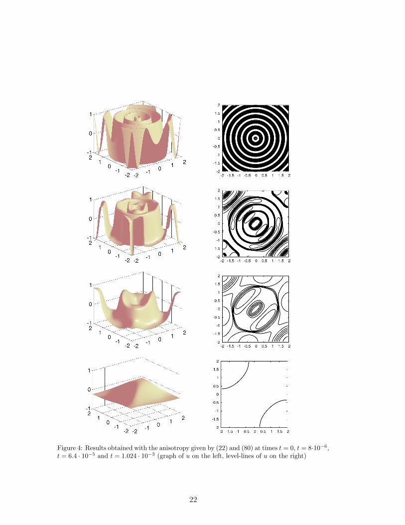
Figure 4: Results obtained with the anisotropy given by (22) and (80) at times t = 0, t = 8·10−6,t = 6.4 · 10−5 and t = 1.024 · 10−3 (graph of u on the left, level-lines of u on the right)

22

Figure 5: Results obtained with the anisotropy given by (23) and εabs − 0.1 at times t = 0,t = 5 · 10−5, t = 0.001 and t = 0.006 – not a steady state (graph of u on the left, level-lines ofu on the right)

23

References

[1] M. Benes, K. Mikula, T. Oberhuber, and D. Sevcovic, Comparison studyfor level set and direct Lagrangian methods for computing Willmore flow ofclosed plannar curves, Computing and Visualization in Science 12 (2009),307–317.

[2] M. Bertalmio, V. Caselles, G. Haro, and G. Sapiro, Handbook of mathemati-cal models in computer vision, ch. PDE-Based Image and Surface Inpainting,pp. 33–61, Springer, 2006.

[3] P.B. Canham, The minimum energy of bending as a possible explanationof biconcave shape of the human red blood cell, J.Theoret.Biol. 26 (1970),61–81.

[4] K. Deckelnick and G. Dziuk, Error estimates for the Willmore flow of graphs,Interfaces Free Bound. 8 (2006), 21–46.

[5] M. Droske and M. Rumpf, A level set formulation for Willmore flow, Inter-faces Free Bound. 6 (2004), no. 3, 361–378.

[6] Q. Du, C. Liu, R. Ryham, and X. Wang, A phase field formulation of theWillmore problem, Nonlinearity (2005), no. 18, 1249–1267.

[7] G. Dziuk, E. Kuwert, and R. Schatzle, Evolution of elastic curves in Rn:Existence and computation, SIAM J. Math. Anal. 41 (2003), no. 6, 2161–2179.

[8] T. Oberhuber, Finite difference scheme for the Willmore flow of graphs,Kybernetika 43 (2007), 855–867.

[9] , Complementary finite volume scheme for the anisotropic surfacediffusion flow, Proceedings of Algoritmy 2009 (A. Handlovicova, P. Frolkovic,K. Mikula, and D. Sevcovic, eds.), 2009, pp. 153–164.

[10] T. Oberhuber, A. Suzuki, and V. Zabka, The cuda implentation of themethod of lines for the curvature dependent flows, Kybernetika 47 (2011),251–272.

[11] T. J. Willmore, Riemannian geometry, Oxford University Press, 2002.

[12] Y. Xu and W. Shu, C., Local discontinuous galerkin method for surface dif-fusion and willmore flow of graphs, Journal of Scientific Computing (2009),375–390.

24