Graphite: Iterative Generative Modeling of Graphs · Graphite: Iterative Generative Modeling of...

Graphite: Iterative Generative Modeling of Graphs

Aditya Grover 1 Aaron Zweig 1 Stefano Ermon 1

AbstractGraphs are a fundamental abstraction for model-ing relational data. However, graphs are discreteand combinatorial in nature, and learning rep-resentations suitable for machine learning tasksposes statistical and computational challenges. Inthis work, we propose Graphite, an algorithmicframework for unsupervised learning of represen-tations over nodes in large graphs using deep la-tent variable generative models. Our model pa-rameterizes variational autoencoders (VAE) withgraph neural networks, and uses a novel iterativegraph refinement strategy inspired by low-rankapproximations for decoding. On a wide varietyof synthetic and benchmark datasets, Graphiteoutperforms competing approaches for the tasksof density estimation, link prediction, and nodeclassification. Finally, we derive a theoretical con-nection between message passing in graph neuralnetworks and mean-field variational inference.

1. IntroductionLatent variable generative modeling is an effective ap-proach for unsupervised representation learning of high-dimensional data (Loehlin, 1998). In recent years, represen-tations learned by latent variable models parameterized bydeep neural networks have shown impressive performanceon many tasks such as semi-supervised learning and struc-tured prediction (Kingma et al., 2014; Sohn et al., 2015).However, these successes have been largely restricted tospecific data modalities such as images and speech. In par-ticular, it is challenging to apply current deep generativemodels for large scale graph-structured data which arise ina wide variety of domains in physical sciences, informationsciences, and social sciences.

To effectively model the relational structure of large graphsfor deep learning, prior works have proposed to use graph

1Department of Computer Science, Stanford University, USA.Correspondence to: Aditya Grover <[email protected]>.

Proceedings of the 36 th International Conference on MachineLearning, Long Beach, California, PMLR 97, 2019. Copyright2019 by the author(s).

neural networks (Gori et al., 2005; Scarselli et al., 2009;Bruna et al., 2013). A graph neural network learns node-level representations by parameterizing an iterative messagepassing procedure between nodes and their neighbors. Thetasks which have benefited from graph neural networks, in-cluding semi-supervised learning (Kipf & Welling, 2017)and few shot learning (Garcia & Bruna, 2018), involve en-coding an input graph to a final output representation (suchas the labels associated with the nodes). The inverse prob-lem of learning to decode a hidden representation into agraph, as in the case of a latent variable generative model,is a pressing challenge that we address in this work.

We propose Graphite, a latent variable generative modelfor graphs based on variational autoencoding (Kingma &Welling, 2014). Specifically, we learn a directed model ex-pressing a joint distribution over the entries of adjacencymatrix of graphs and latent feature vectors for every node.Our framework uses graph neural networks for inference(encoding) and generation (decoding). While the encodingis straightforward and can use any existing graph neural net-work, the decoding of these latent features to reconstruct theoriginal graph is done using a multi-layer iterative procedure.The procedure starts with an initial reconstruction based onthe inferred latent features, and iteratively refines the re-constructed graph via a message passing operation. Theiterative refinement can be efficiently implemented usinggraph neural networks. In addition to the Graphite model,we also contribute to the theoretical understanding of graphneural networks by deriving equivalences between messagepassing in graph neural networks with mean-field inferencein latent variable models via kernel embeddings (Smolaet al., 2007; Dai et al., 2016), formalizing what has thus farhas been largely speculated empirically to the best of ourknowledge (Yoon et al., 2018).

In contrast to recent works focussing on generation of smallgraphs e.g., molecules (You et al., 2018; Li et al., 2018), theGraphite framework is particularly suited for representationlearning on large graphs. Such representations are useful forseveral downstream tasks. In particular, we demonstrate thatrepresentations learned via Graphite outperform competingapproaches for graph representation learning empiricallyfor the tasks of density estimation (over entire graphs), linkprediction, and semi-supervised node classification on syn-thetic and benchmark datasets.

arX

iv:1

803.

1045

9v4

[st

at.M

L]

15

May

201

9


2. PreliminariesThroughout this work, we assume that all probability distri-butions admit absolutely continuous densities on a suitablereference measure. Consider a weighted undirected graphG = (V,E) where V and E denote index sets of nodes andedges respectively. Additionally, we denote the (optional)feature matrix associated with the graph as X ∈ Rn×m foran m-dimensional signal associated with each node, for e.g.,these could refer to the user attributes in a social network.We represent the graph structure using a symmetric adja-cency matrix A ∈ Rn×n where n = |V | and the entries Aijdenote the weight of the edge between node i and j.

2.1. Weisfeiler-Lehman algorithm

The Weisfeiler-Lehman (WL) algorithm (Weisfeiler &Lehman, 1968; Douglas, 2011) is a heuristic test of graphisomorphism between any two graphs G and G′. The algo-rithm proceeds in iterations. Before the first iteration, welabel every node in G and G′ with a scalar isomorphisminvariant initialization (e.g., node degrees). That is, if Gand G′ are assumed to be isomorphic, then an isomorphisminvariant initialization is one where the matching nodesestablishing the isomorphism in G and G′ have the samelabels (a.k.a. messages). Let H(0) = [h

(l)1 , h

(l)2 , · · · , h(l)n ]T

denote the vector of initializations for the nodes in the graphat iteration l ∈ N∪0. At every iteration l > 0, we perform arelabelling of nodes inG andG′ based on a message passingupdate rule:

H(l) ← hash(AH(l−1)

)(1)

where A denotes the adjacency matrix of the correspondinggraph and hash : Rn → Rn is any suitable hash functione.g., a non-linear activation. Hence, the message for everynode is computed as a hashed sum of the messages fromthe neighboring nodes (since Aij 6= 0 only if i and j areneighbors). We repeat the process for a specified numberof iterations, or until convergence. If the label sets for thenodes in G and G′ are equal (which can be checked usingsorting in O(n log n) time), then the algorithm declares thetwo graphs G and G′ to be isomorphic.

The “k-dim” WL algorithm extends the 1-dim algorithmabove by simultaneously passing messages of length k (eachinitialized with some isomorphism invariant scheme). Apositive test for isomorphism requires equality in all k di-mensions for nodes in G and G′ after the termination ofmessage passing. This algorithmic test is a heuristic whichguarantees no false negatives but can give false positiveswherein two non-isomorphic graphs can be falsely declaredisomorphic. Empirically, the test has been shown to failon some regular graphs but gives excellent performance onreal-world graphs (Shervashidze et al., 2011).

2.2. Graph neural networks

Intuitively, the WL algorithm encodes the structure of thegraph in the form of messages at every node. Graph neuralnetworks (GNN) build on this observation and parameterizean unfolding of the iterative message passing procedurewhich we describe next.

A GNN consists of many layers, indexed by l ∈ N with eachlayer associated with an activation ηl and a dimensionalitydl. In addition to the input graph A, every layer l ∈ N ofthe GNN takes as input the activations from the previouslayer H(l−1) ∈ Rn×dl−1 , a family of linear transformationsFl : Rn×n → Rn×n, and a matrix of learnable weightparameters Wl ∈ Rdl−1×dl and optional bias parametersBl ∈ Rn×dl . Recursively, the layer wise propagation rulein a GNN is given by:

H(l) ← ηl

Bl +∑f∈Fl

f(A)H(l−1)Wl

(2)

with the base cases H(0) = X and d0 = m. Here, m is thefeature dimensionality. If there are no explicit node features,we set H(0) = In (identity) and d0 = n. Several variantsof graph neural networks have been proposed in prior work.For instance, graph convolutional networks (GCN) (Kipf& Welling, 2017) instantiate graph neural networks with apermutation equivariant propagation rule:

H(l) ← ηl

(Bl + AH(l−1)Wl

)(3)

where A = D−1/2AD−1/2 is the symmetric diagonal-ization of A given the diagonal degree matrix D (i.e.,Dii =

∑(i,j)∈E Aij), and same base cases as before. Com-

paring the above with the WL update rule in Eq. (1), wecan see that the activations for every layer in a GCN arecomputed via parameterized, scaled activations (messages)of the previous layer being propagated over the graph, withthe hash function implicitly specified using an activationfunction ηl.

Our framework is agnostic to instantiations of messagepassing rule of a graph neural network in Eq. (2), and weuse graph convolutional networks for experimental vali-dation due to the permutation equivariance property. Forbrevity, we denote the output H for the final layer of amulti-layer graph neural network with input adjacency ma-trix A, node feature matrix X, and parameters 〈W,B〉 asH = GNN〈W,B〉(A,X), with appropriate activation func-tions and linear transformations applied at each hidden layerof the network.

3. Generative Modeling via GraphiteFor generative modeling of graphs, we are interested inlearning a parameterized distribution over adjacency matri-


Figure 1. Latent variable model for Graphite. Observed evidencevariables in gray.

ces A. In this work, we restrict ourselves to modeling graphstructure only, and any additional information in the form ofnode features X is incorporated as conditioning evidence.

In Graphite, we adopt a latent variable approach for model-ing the generative process. That is, we introduce latentvariable vectors Zi ∈ Rk and evidence feature vectorsXi ∈ Rm for each node i ∈ {1, 2, · · · , n} along withan observed variable for each pair of nodes Aij ∈ R. Un-less necessary, we use a succinct representation Z ∈ Rn×k,X ∈ Rn×m, and A ∈ Rn×n for the variables henceforth.The conditional independencies between the variables canbe summarized in the directed graphical model (using platenotation) in Figure 1. We can learn the model parametersθ by maximizing the marginal likelihood of the observedadjacency matrix conditioned on X:

maxθ

log pθ(A|X) = log

∫Z

pθ(A,Z|X)dZ (4)

Here, p(Z|X) is a fixed prior distribution over the latentfeatures of every node e.g., isotropic Gaussian. If we havemultiple graphs in our dataset, we maximize the expectedlog-likelihoods over all the corresponding adjacency matri-ces. We can obtain a tractable, stochastic evidence lowerbound (ELBO) to the above objective by introducing a vari-ational posterior qφ(Z|A,X) with parameters φ:

log pθ(A|X) ≥ Eqφ(Z|A,X)

[log

pθ(A,Z|X)

qφ(Z|A,X)

](5)

The lower bound is tight when the variational posteriorqφ(Z|A,X) matches the true posterior pθ(Z|A,X) andhence maximizing the above objective optimizes for theparameters that define the best approximation to the trueposterior within the variational family (Blei et al., 2017). Wenow discuss parameterizations for specifying qφ(Z|A,X)(i.e., encoder) and pθ(A|Z,X) (i.e., decoder).

Encoding using forward message passing. Typically weuse the mean field approximation for defining the variationalfamily and hence:

qφ(Z|A,X) ≈n∏i=1

qφi(Zi|A,X) (6)

Additionally, we would like to make distributional assump-tions on each variational marginal density qφi(Zi|A,X)such that it is reparameterizable and easy-to-sample, suchthat the gradients w.r.t. φi have low variance (Kingma &Welling, 2014). In Graphite, we assume isotropic Gaussianvariational marginals with diagonal covariance. The parame-ters for the variational marginals qφi(Z|A,X) are specifiedusing a graph neural network:

µ,σ = GNNφ(A,X) (7)

where µ and σ denote the vector of means and standarddeviations for the variational marginals {qφi(Zi|A,X)}ni=1

and φ = {φi}ni=1 are the full set of variational parameters.

Decoding using reverse message passing. For specify-ing the observation model pθ(A|Z,X), we cannot directlyuse a graph neural network since we do not have an inputgraph for message passing. To sidestep this issue, we pro-pose an iterative two-step approach that alternates betweendefining an intermediate graph and then gradually refiningthis graph through message passing. Formally, given a latentmatrix Z and an input feature matrix X, we iterate over thefollowing sequence of operations:

A =ZZT

‖Z‖2+ 11T , (8)

Z∗ = GNNθ(A, [Z|X]) (9)

where the second argument to the GNN is a concatenation ofZ and X. The first step constructs an intermediate weightedgraph A ∈ Rn×n by applying an inner product of Z withitself and adding an additional constant of 1 to ensure en-tries are non-negative. And the second step performs a passthrough a parameterized graph neural network. We canrepeat the above sequence to gradually refine the featurematrix Z∗. The final distribution over graph parameters isobtained using an inner product step on Z∗ ∈ Rn×k∗ akin toEq. (8), where k∗ ∈ N is determined via the network archi-tecture. For efficient sampling, we assume the observationmodel factorizes:

pθ(A|Z,X) =

n∏i=1

n∏j=1

p(i,j)θ (Aij |Z∗). (10)

The distribution over the individual edges can be expressedas a Bernoulli or Gaussian distribution for unweighted andreal-valued edges respectively. E.g., the edge probabilitiesfor an unweighted graph are given as sigmoid(Z∗Z∗

T

).


Table 1. Mean reconstruction errors and negative log-likelihood estimates (in nats) for autoencoders and variational autoencodersrespectively on test instances from six different generative families. Lower is better.

Erdos-Renyi Ego Regular Geometric Power Law Barabasi-Albert

GAE 221.79 ± 7.58 197.3 ± 1.99 198.5 ± 4.78 514.26 ± 41.58 519.44 ± 36.30 236.29 ± 15.13Graphite-AE 195.56 ± 1.49 182.79 ± 1.45 191.41 ± 1.99 181.14 ± 4.48 201.22 ± 2.42 192.38 ± 1.61

VGAE 273.82 ± 0.07 273.76 ± 0.06 275.29 ± 0.08 274.09 ± 0.06 278.86 ± 0.12 274.4 ± 0.08Graphite-VAE 270.22 ± 0.15 270.70 ± 0.32 266.54 ± 0.12 269.71 ± 0.08 263.92 ± 0.14 268.73 ± 0.09

3.1. Scalable learning & inference in Graphite

For representation learning of large graphs, we require theencoding and decoding steps in Graphite to be computation-ally efficient. On the surface, the decoding step involvesinner products of potentially dense matrices Z, which is anO(n2k) operation. Here, k is the dimension of the per-nodelatent vectors Zi used to define A.

For any intermediate decoding step as in Eq. (8), we proposeto offset this expensive computation by using the associa-tivity property of matrix multiplications for the messagepassing step in Eq. (9). For notational brevity, consider thesimplified graph propagation rule for a GNN:

H(l) ← ηl

(AH(l−1)

)where A is defined in Eq. (8).

Instead of directly taking an inner product of Z with it-self, we note that the subsequent operation involves anothermatrix multiplication and hence, we can perform right mul-tiplication instead. If dl and dl−1 denote the size of thelayers H(l) and H(l−1) respectively, then the time complex-ity of propagation based on right multiplication is given byO(nkdl−1 + ndl−1dl).

The above trick sidesteps the quadratic n2 complexity fordecoding in the intermediate layers without any loss in sta-tistical accuracy. The final layer however still involves aninner product with respect to Z∗ between potentially densematrices. However, since the edges are generated indepen-dently, we can approximate the loss objective by performinga Monte Carlo evaluation of the reconstructed adjacencymatrix parameters in Eq. (10). By adaptively choosing thenumber of entries for Monte Carlo approximation, we cantrade-off statistical accuracy for computational budget.

4. Experimental EvaluationWe evaluate Graphite on tasks involving entire graphs,nodes, and edges. We consider two variants of our pro-posed framework: the Graphite-VAE, which corresponds toa directed latent variable model as described in Section 3 andGraphite-AE, which corresponds to an autoencoder trained

to minimize the error in reconstructing an input adjacencymatrix. For unweighted graphs (i.e., A ∈ {0, 1}n×n), thereconstruction terms in the objectives for both Graphite-VAE and Graphite-AE minimize the negative cross entropybetween the input and reconstructed adjacency matrices. Forweighted graphs, we use the mean squared error. Additionalhyperparameter details are described in Appendix B.

4.1. Reconstruction & density estimation

In the first set of tasks, we evaluate learning in Graphitebased on held-out reconstruction losses and log-likelihoodsestimated by the learned Graphite-VAE and Graphite-AEmodels respectively on a collection of graphs with varyingsizes. In direct contrast to modalities such as images, graphscannot be straightforwardly reduced to a fixed number ofvertices for input to a graph convolutional network. Onesimplifying modification taken by Bojchevski et al. (2018)is to consider only the largest connected component forevaluating and optimizing the objective, which we appealto as well. Thus by setting the dimensions of Z∗ to a maxi-mum number of vertices, Graphite can be used for inferencetasks over entire graphs with potentially smaller sizes byconsidering only the largest connected component.

We create datasets from six graph families with fixed,known generative processes: the Erdos-Renyi, ego-nets,random regular graphs, random geometric graphs, randomPower Law Tree and Barabasi-Albert. For each family, 300graph instances were sampled with each instance having10− 20 nodes and evenly split into train/validation/test in-stances. As a benchmark comparison, we compare againstthe Graph Autoencoder/Variational Graph Autoencoder(GAE/VGAE) (Kipf & Welling, 2016). The GAE/VGAEmodels consist of an encoding procedure similar to Graphite.However, the decoder has no learnable parameters and re-construction is done solely through an inner product opera-tion (such as the one in Eq. (8)).

The mean reconstruction errors and the negative log-likelihood results on a test set of instances are shown inTable 1. Both Graphite-AE and Graphite-VAE outperformAE and VGAE significantly on these tasks, indicating theusefulness of learned decoders in Graphite.


Table 2. Citation network statistics

Nodes Edges Node Features Labels

Cora 2708 5429 1433 7Citeseer 3327 4732 3703 6Pubmed 19717 44338 500 3

4.2. Link prediction

The task of link prediction is to predict whether an edgeexists between a pair of nodes (Loehlin, 1998). Even thoughGraphite learns a distribution over graphs, it can be used forpredictive tasks within a single graph. In order to do so, welearn a model for a random, connected training subgraph ofthe true graph. For validation and testing, we add a balancedset of positive and negative (false) edges to the originalgraph and evaluate the model performance based on thereconstruction probabilities assigned to the validation andtest edges (similar to denoising of the input graph). In ourexperiments, we held out a set of 5% edges for validation,10% edges for testing, and train all models on the remainingsubgraph. Additionally, the validation and testing sets alsoeach contain an equal number of non-edges.

Datasets. We compared across standard benchmark cita-tion network datasets: Cora, Citeseer, and Pubmed withpapers as nodes and citations as edges (Sen et al., 2008).The node-level features correspond to the text attributes inthe papers. The dataset statistics are summarized in Table 2.

Baselines and evaluation metrics. We evaluate perfor-mance based on the Area Under the ROC Curve (AUC) andAverage Precision (AP) metrics. We evaluated Graphite-VAE and Graphite-AE against the following baselines: Spec-tral Clustering (SC) (Tang & Liu, 2011), DeepWalk (Per-ozzi et al., 2014), node2vec (Grover & Leskovec, 2016),and GAE/VGAE (Kipf & Welling, 2016). SC, DeepWalk,and node2vec do not provide the ability to incorporate nodefeatures while learning embeddings, and hence we evaluatethem only on the featureless datasets.

Results. The AUC and AP results (along with standarderrors) are shown in Table 3 and Table 4 respectively aver-aged over 50 random train/validation/test splits. On bothmetrics, Graphite-VAE gives the best performance overall.Graphite-AE also gives good results, generally outperform-ing its closest competitor GAE.

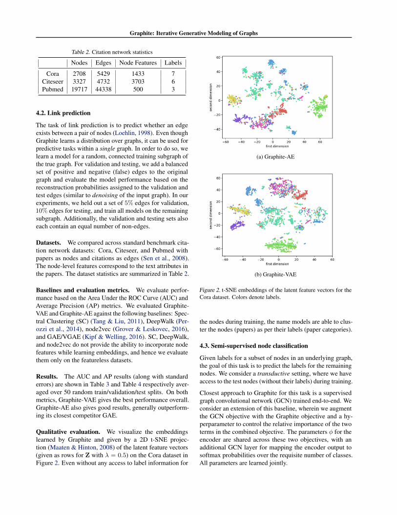
Qualitative evaluation. We visualize the embeddingslearned by Graphite and given by a 2D t-SNE projec-tion (Maaten & Hinton, 2008) of the latent feature vectors(given as rows for Z with λ = 0.5) on the Cora dataset inFigure 2. Even without any access to label information for

(a) Graphite-AE

(b) Graphite-VAE

Figure 2. t-SNE embeddings of the latent feature vectors for theCora dataset. Colors denote labels.

the nodes during training, the name models are able to clus-ter the nodes (papers) as per their labels (paper categories).

4.3. Semi-supervised node classification

Given labels for a subset of nodes in an underlying graph,the goal of this task is to predict the labels for the remainingnodes. We consider a transductive setting, where we haveaccess to the test nodes (without their labels) during training.

Closest approach to Graphite for this task is a supervisedgraph convolutional network (GCN) trained end-to-end. Weconsider an extension of this baseline, wherein we augmentthe GCN objective with the Graphite objective and a hy-perparameter to control the relative importance of the twoterms in the combined objective. The parameters φ for theencoder are shared across these two objectives, with anadditional GCN layer for mapping the encoder output tosoftmax probabilities over the requisite number of classes.All parameters are learned jointly.


Table 3. Area Under the ROC Curve (AUC) for link prediction (* denotes dataset with features). Higher is better.

Cora Citeseer Pubmed Cora* Citeseer* Pubmed*

SC 89.9 ± 0.20 91.5 ± 0.17 94.9 ± 0.04 - - -DeepWalk 85.0 ± 0.17 88.6 ± 0.15 91.5 ± 0.04 - - -node2vec 85.6 ± 0.15 89.4 ± 0.14 91.9 ± 0.04 - - -

GAE 90.2 ± 0.16 92.0 ± 0.14 92.5 ± 0.06 93.9 ± 0.11 94.9 ± 0.13 96.8 ± 0.04VGAE 90.1 ± 0.15 92.0 ± 0.17 92.3 ± 0.06 94.1 ± 0.11 96.7 ± 0.08 95.5 ± 0.13

Graphite-AE 91.0 ± 0.15 92.6 ± 0.16 94.5 ± 0.05 94.2 ± 0.13 96.2 ± 0.10 97.8 ± 0.03Graphite-VAE 91.5 ± 0.15 93.5 ± 0.13 94.6 ± 0.04 94.7 ± 0.11 97.3 ± 0.06 97.4 ± 0.04

Table 4. Average Precision (AP) scores for link prediction (* denotes dataset with features). Higher is better.

Cora Citeseer Pubmed Cora* Citeseer* Pubmed*

SC 92.8 ± 0.12 94.4 ± 0.11 96.0 ± 0.03 - - -DeepWalk 86.6 ± 0.17 90.3 ± 0.12 91.9 ± 0.05 - - -node2vec 87.5 ± 0.14 91.3 ± 0.13 92.3 ± 0.05 - - -

GAE 92.4 ± 0.12 94.0 ± 0.12 94.3 ± 0.5 94.3 ± 0.12 94.8 ± 0.15 96.8 ± 0.04VGAE 92.3 ± 0.12 94.2 ± 0.12 94.2 ± 0.04 94.6 ± 0.11 97.0 ± 0.08 95.5 ± 0.12

Graphite-AE 92.8 ± 0.13 94.1 ± 0.14 95.7 ± 0.06 94.5 ± 0.14 96.1 ± 0.12 97.7 ± 0.03Graphite-VAE 93.2 ± 0.13 95.0 ± 0.10 96.0 ± 0.03 94.9 ± 0.13 97.4 ± 0.06 97.4 ± 0.04

Table 5. Classification accuracies (* denotes dataset with features).Baseline numbers from Kipf & Welling (2017).

Cora* Citeseer* Pubmed*

SemiEmb 59.0 59.6 71.1DeepWalk 67.2 43.2 65.3

ICA 75.1 69.1 73.9Planetoid 75.7 64.7 77.2

GCN 81.5 70.3 79.0

Graphite 82.1 ± 0.06 71.0 ± 0.07 79.3 ± 0.03

Results. The classification accuracy of the semi-supervised models is given in Table 5. We find that Graphite-hybrid outperforms the competing models on all datasetsand in particular the GCN approach which is the closestbaseline. Recent work in Graph Attention Networks showsthat extending GCN by incoporating attention can boostperformance on this task (Velickovic et al., 2018). UsingGATs in place of GCNs for parameterizing Graphite couldyield similar performance boost in future work.

5. Theoretical AnalysisIn this section, we derive a theoretical connection betweenmessage passing in graph neural networks and approximateinference in related undirected graphical models.

5.1. Kernel embeddings

We first provide a brief background on kernel embeddings.A kernel defines a notion of similarity between pairs ofobjects (Scholkopf & Smola, 2002; Shawe-Taylor & Cris-tianini, 2004). Let K : Z × Z → R be the kernel functiondefined over a space of objects, say Z . With every kernelfunction K, we have an associated feature map ψ : Z → HwhereH is a potentially infinite dimensional feature space.

Kernel methods can be used to specify embeddings of dis-tributions of arbitrary objects (Smola et al., 2007; Grettonet al., 2007). Formally, we denote these functional map-pings as Tψ : P → H where P specifies the space of alldistributions on Z . These mappings, referred to as kernelembeddings of distributions, are defined as:

Tψ(p) := EZ∼p[ψ(Z)] (11)

for any p ∈ P . We are particularly interested in kernels withfeature maps ψ that define injective embeddings, i.e., for anypair of distributions p1 and p2, we have Tψ(p1) 6= Tψ(p2)if p1 6= p2. For injective embeddings, we can computefunctionals of any distribution by directly applying a cor-responding function on its embedding. Formally, for everyfunction O : P → Rd, d ∈ N and injective embedding Tψ,there exists a function Oψ : H → Rd such that:

O(p) = Oψ(Tψ(p)) ∀p ∈ P. (12)

Informally, we can see that the operator Oψ can be definedas the composition of O with the inverse of Tψ .


2 3

1

(a) Input graph with edge set E = {(1, 2), (1, 3)}.

X2 Z2 X3Z3

X1

Z1

A12

A23

A13

(b) Latent variable model G satisfying Property 1 with A12 6=0,A23 = 0,A13 6= 0.

Figure 3. Interpreting message passing in Graph Neural Networksvia Kernel Embeddings and Mean-field inference

5.2. Connections with mean-field inference

Locality preference for representational learning is a keyinductive bias for graphs. We formulate this using an (undi-rected) graphical model G over X, A, and {Z1, · · · ,Zn}.As in a GNN, we assume that X and A are observedand specify conditional independence structure in a con-ditional distribution over the latent variables, denoted asr(Z1, · · · ,Zn|A,X). We are particularly interested in mod-els that satisfy the following property.

Property 1. The edge set E defined by the adjacencymatrix A is an undirected I-map for the distributionr(Z1, · · · ,Zn|A,X).

In words, the above property implies that according to theconditional distribution over Z, any individual Zi is inde-pendent of all other Zj when conditioned on A, X, and theneighboring latent variables of node i as determined by theedge set E. See Figure 3 for an illustration.

A mean-field (MF) approximation for G approximates theconditional distribution r(Z1, · · · ,Zn|A,X) as:

r(Z1, · · · ,Zn|A,X) ≈n∏i=1

qφi(Zi|A,X) (13)

where φi denotes the set of parameters for the i-th varia-tional marginal. These parameters are optimized by mini-mizing the KL-divergence between the variational and thetrue conditional distributions:

minφ1,··· ,φn

KL

(n∏i=1

qφi (Zi|A,X)‖r(Z1, · · · ,Zn|A,X)

)(14)

Using standard variational arguments (Wainwright et al.,2008), we know that the optimal variational marginals as-sume the following functional form:

qφi(Zi|A,X) = OMFG

(Zi, {qφj}j∈N (i)

)(15)

where N (i) denotes the neighbors of Zi in G and O is afunction determined by the fixed point equations that de-pends on the potentials associated with G. Importantly, theabove functional form suggests that the optimal marginalsin mean field inference are locally consistent that they areonly a function of the neighboring marginals. An iterativealgorithm for mean-field inference is to perform messagepassing over the underlying graph until convergence. Withan appropriate initialization at l = 0, the updated marginalsat iteration l ∈ N are given as:

q(l)φi(Zi|A,X) = OMF

G

(Zi, {q(l−1)φj

}j∈N (i)

). (16)

We will sidestep deriving O, and instead use the kernelembeddings of the variational marginals to directly rea-son in the embedding space. That is, we assume we havean injective embedding for each marginal qφi given byµi = EZi∼qφi [ψ(Zi)] for some feature map ψ : Rk → Rk′

and directly use the equivalence established in Eq. (12) it-eratively. For mean-field inference via message passing asin Eq. (16), this gives us the following recursive expressionfor iteratively updating the embeddings at iteration l ∈ N:

µ(l)i = OMF

ψ,G

({µ(l−1)

j }j∈N (i)

)(17)

with an appropriate base case for µ(0)i . We then have the

following result:

Theorem 2. Let G be any undirected latent variable modelsuch that the conditional distribution r(Z1, · · · ,Zn|A,X)expressed by the model satisfies Property 1.

Then there exists a choice of ηl, Fl, Wl, and Bl such thatfor all {µ(l−1)

i }ni=1, the GNN propagation rule in Eq. (2) iscomputationally equivalent to updating {µ(l−1)

i }ni=1 via afirst order approximation of Eq. (17).

Proof. See Appendix A.

While ηl and Fl are typically fixed beforehand, the parame-ters Wl, and Bl are directly learned from data in practice.Hence we have shown that a GNN is a good model forcomputation with respect to latent variable models that at-tempt to capture inductive biases relevant to graphs, i.e.,ones where the latent feature vector for every node is condi-tionally independent from everything else given the featurevectors of its neighbors (and A, X). Note that such a graphi-cal model would satisfy Property 1 but is in general different


from the posterior specified by the one in Figure 1. Howeverif the true (but unknown) posterior on the latent variablesfor the model proposed in Figure 1 could be expressed as anequivalent model satisfying the desired property, then Theo-rem 2 indeed suggests the use of GNNs for parameterizingvariational posteriors, as we do so in the case of Graphite.

6. Discussion & Related WorkOur framework effectively marries probabilistic modelingand representation learning on graphs. We review some ofthe dominant prior works in these fields below.

Probabilistic modeling of graphs. The earliest proba-bilistic models of graphs proposed to generate graphs bycreating an edge between any pair of nodes with a constantprobability (Erdos & Renyi, 1959). Several alternatives havebeen proposed since; e.g., the small-world model generatesgraphs that exhibit local clustering (Watts & Strogatz, 1998),the Barabasi-Albert models preferential attachment whereinhigh-degree nodes are likely to form edges with newly addednodes (Barabasi & Albert, 1999), the stochastic block modelis based on inter and intra community linkages (Hollandet al., 1983) etc. We direct the interested reader to prominentsurveys on this topic (Newman, 2003; Mitzenmacher, 2004;Chakrabarti & Faloutsos, 2006).

Representation learning on graphs. For representationlearning on graphs, there are broadly three kinds of ap-proaches: matrix factorization, random walk based ap-proaches, and graph neural networks. We include a briefdiscussion on the first two kinds in Appendix C and referthe reader to Hamilton et al. (2017b) for a recent survey.

Graph neural networks, a collective term for networks thatoperate over graphs using message passing, have shown suc-cess on several downstream applications, e.g., (Duvenaudet al., 2015; Li et al., 2016; Kearnes et al., 2016; Kipf &Welling, 2017; Hamilton et al., 2017a) and the referencestherein. Gilmer et al. (2017) provides a comprehensivecharacterization of these networks in the message passingsetup. We used Graph Convolution Networks, partly to pro-vide a direct comparison with GAE/VGAE and leave theexploration of other GNN variants for future work.

Latent variable models for graphs. HierarchicalBayesian models parameterized by deep neural networkshave been recently proposed for graphs (Hu et al., 2017;Wang et al., 2017). Besides being restricted to singlegraphs, these models are limited since inference requiresrunning expensive Markov chains (Hu et al., 2017) or aretask-specific (Wang et al., 2017). Johnson (2017) andKipf et al. (2018) generate graphs as latent representationslearned directly from data. In contrast, we are interested

in modeling observed (and not latent) relational structure.Finally, there has been a fair share of recent work forgeneration of special kinds of graphs, such as parsed treesof source code (Maddison & Tarlow, 2014) and SMILESrepresentations for molecules (Olivecrona et al., 2017).

Several deep generative models for graphs have recentlybeen proposed. Amongst adversarial generation approaches,Wang et al. (2018) and Bojchevski et al. (2018) model localgraph neighborhoods and random walks on graphs respec-tively. Li et al. (2018) and You et al. (2018) model graphsas sequences and generate graphs via autoregressive pro-cedures. Adversarial and autoregressive approaches aresuccessful at generating graphs, but do not directly allowfor inferring latent variables via encoders. Latent variablegenerative models have also been proposed for generatingsmall molecular graphs (Jin et al., 2018; Samanta et al.,2018; Simonovsky & Komodakis, 2018). These methodsinvolve an expensive decoding procedure that limits scalingto large graphs. Finally, closest to our framework is theGAE/VGAE approach (Kipf & Welling, 2016) discussedin Section 4. Pan et al. (2018) extends this approach withan adversarial regularization framework but retain the innerproduct decoder. Our work proposes a novel multi-stepdecoding mechanism based on graph refinement.

7. Conclusion & Future WorkWe proposed Graphite, a scalable deep generative modelfor graphs based on variational autoencoding. The encodersand decoders in Graphite are parameterized by graph neuralnetworks that propagate information locally on a graph. Ourproposed decoder performs a multi-layer iterative decod-ing comprising of alternate inner product operations andmessage passing on the intermediate graph.

Current generative models for graphs are not permutation-invariant and are learned by feeding graphs with a fixed orheuristic ordering of nodes. This is an exciting challenge forfuture work, which could potentially be resolved by incor-porate graph representations robust to permutation invari-ances (Verma & Zhang, 2017) or modeling distributions overpermutations of node orderings via recent approaches suchas NeuralSort (Grover et al., 2019). Extending Graphitefor modeling richer graphical structure such as heteroge-neous and time-varying graphs, as well as integrating do-main knowledge within Graphite decoders for applicationsin generative design and synthesis e.g., molecules, programs,and parse trees is another interesting future direction.

Finally, our theoretical results in Section 5 suggest that aprincipled design of layerwise propagation rules in graphneural networks inspired by additional message passinginference schemes (Dai et al., 2016; Gilmer et al., 2017) isanother avenue for future research.


AcknowledgementsThis research has been supported by Siemens, a Futureof Life Institute grant, NSF grants (#1651565, #1522054,#1733686), ONR (N00014-19-1-2145), AFOSR (FA9550-19-1-0024), and an Amazon AWS Machine Learning Grant.AG is supported by a Microsoft Research Ph.D. fellowshipand a Stanford Data Science Scholarship. We would like tothank Daniel Levy for helpful comments on early drafts.

ReferencesBarabasi, A.-L. and Albert, R. Emergence of scaling in

random networks. Science, 286(5439):509–512, 1999.

Belkin, M. and Niyogi, P. Laplacian eigenmaps and spectraltechniques for embedding and clustering. In Advances inNeural Information Processing Systems, 2002.

Blei, D. M., Kucukelbir, A., and McAuliffe, J. D. Varia-tional inference: A review for statisticians. Journal ofthe American Statistical Association, 112(518):859–877,2017.

Bojchevski, A., Shchur, O., Zugner, D., and Gunnemann,S. NetGAN: Generating graphs via random walks. InInternational Conference on Machine Learning, 2018.

Bruna, J., Zaremba, W., Szlam, A., and LeCun, Y. Spectralnetworks and locally connected networks on graphs. InInternational Conference on Learning Representations,2013.

Chakrabarti, D. and Faloutsos, C. Graph mining: Laws,generators, and algorithms. ACM Computing Surveys, 38(1):2, 2006.

Dai, H., Dai, B., and Song, L. Discriminative embeddings oflatent variable models for structured data. In InternationalConference on Machine Learning, 2016.

Douglas, B. L. The Weisfeiler-Lehman method and graphisomorphism testing. arXiv preprint arXiv:1101.5211,2011.

Duvenaud, D., Maclaurin, D., Iparraguirre, J., Bombarell,R., Hirzel, T., Aspuru-Guzik, A., and Adams, R. Convo-lutional networks on graphs for learning molecular fin-gerprints. In Advances in Neural Information ProcessingSystems, 2015.

Erdos, P. and Renyi, A. On random graphs. PublicationesMathematicae (Debrecen), 6:290–297, 1959.

Garcia, V. and Bruna, J. Few-shot learning with graph neu-ral networks. In International Conference on LearningRepresentations, 2018.

Gilmer, J., Schoenholz, S., Riley, P., Vinyals, O., and Dahl,G. Neural message passing for quantum chemistry. InInternational Conference on Machine Learning, 2017.

Gori, M., Monfardini, G., and Scarselli, F. A new modelfor learning in graph domains. In International JointConference on Neural Networks, 2005.

Gretton, A., Borgwardt, K., Rasch, M., Scholkopf, B., andSmola, A. A kernel method for the two-sample-problem.In Advances in Neural Information Processing Systems,2007.

Grover, A. and Leskovec, J. node2vec: Scalable featurelearning for networks. In Knowledge Discovery and DataMining, 2016.

Grover, A., Wang, E., Zweig, A., and Ermon, S. Stochasticoptimization of sorting networks via continuous relax-ations. In International Conference on Learning Repre-sentations, 2019.

Hamilton, W., Ying, Z., and Leskovec, J. Inductive repre-sentation learning on large graphs. In Advances in NeuralInformation Processing Systems, 2017a.

Hamilton, W. L., Ying, R., and Leskovec, J. Representationlearning on graphs: Methods and applications. arXivpreprint arXiv:1709.05584, 2017b.

Holland, P. W., Laskey, K. B., and Leinhardt, S. Stochasticblockmodels: First steps. Social networks, 5(2):109–137,1983.

Hu, C., Rai, P., and Carin, L. Deep generative models forrelational data with side information. In InternationalConference on Machine Learning, 2017.

Jin, W., Barzilay, R., and Jaakkola, T. Junction tree vari-ational autoencoder for molecular graph generation. InInternatiional Conference on Machine Learning, 2018.

Johnson, D. Learning graphical state transitions. In Interna-tional Conference on Learning Representations, 2017.

Kearnes, S., McCloskey, K., Berndl, M., Pande, V., andRiley, P. Molecular graph convolutions: moving beyondfingerprints. Journal of computer-aided molecular design,30(8):595–608, 2016.

Kingma, D. P. and Welling, M. Auto-encoding variationalbayes. In International Conference on Learning Repre-sentations, 2014.

Kingma, D. P., Mohamed, S., Rezende, D. J., and Welling,M. Semi-supervised learning with deep generative mod-els. In Advances in Neural Information Processing Sys-tems, 2014.


Kipf, T., Fetaya, E., Wang, K.-C., Welling, M., and Zemel,R. Neural relational inference for interacting systems. InInternational Conference on Machine Learning, 2018.

Kipf, T. N. and Welling, M. Variational graph auto-encoders.arXiv preprint arXiv:1611.07308, 2016.

Kipf, T. N. and Welling, M. Semi-supervised classifica-tion with graph convolutional networks. In InternationalConference on Learning Representations, 2017.

Li, Y., Tarlow, D., Brockschmidt, M., and Zemel, R. Gatedgraph sequence neural networks. In International Con-ference on Learning Representations, 2016.

Li, Y., Vinyals, O., Dyer, C., Pascanu, R., and Battaglia,P. Learning deep generative models of graphs. arXivpreprint arXiv:1803.03324, 2018.

Loehlin, J. C. Latent variable models: An introduction tofactor, path, and structural analysis. Lawrence ErlbaumAssociates Publishers, 1998.

Lu, Q. and Getoor, L. Link-based classification. In Interna-tional Conference on Machine Learning, 2003.

Maaten, L. v. d. and Hinton, G. Visualizing data usingt-sne. Journal of Machine Learning Research, 9(Nov):2579–2605, 2008.

Maddison, C. and Tarlow, D. Structured generative modelsof natural source code. In International Conference onMachine Learning, 2014.

Mikolov, T., Sutskever, I., Chen, K., Corrado, G. S., andDean, J. Distributed representations of words and phrasesand their compositionality. In Advances in Neural Infor-mation Processing Systems, 2013.

Mitzenmacher, M. A brief history of generative models forpower law and lognormal distributions. Internet mathe-matics, 1(2):226–251, 2004.

Newman, M. E. The structure and function of complexnetworks. SIAM review, 45(2):167–256, 2003.

Olivecrona, M., Blaschke, T., Engkvist, O., and Chen, H.Molecular de-novo design through deep reinforcementlearning. Journal of cheminformatics, 9(1):48, 2017.

Pan, S., Hu, R., Long, G., Jiang, J., Yao, L., and Zhang, C.Adversarially regularized graph autoencoder for graphembedding. In International Joint Conference on Artifi-cial Intelligence, 2018.

Pedregosa, F., Varoquaux, G., Gramfort, A., Michel, V.,Thirion, B., Grisel, O., Blondel, M., Prettenhofer, P.,Weiss, R., Dubourg, V., et al. Scikit-learn: Machine learn-ing in python. Journal of Machine Learning Research,12(Oct):2825–2830, 2011.

Perozzi, B., Al-Rfou, R., and Skiena, S. Deepwalk: On-line learning of social representations. In KnowledgeDiscovery and Data Mining, 2014.

Samanta, B., De, A., Ganguly, N., and Gomez-Rodriguez,M. Designing random graph models using variationalautoencoders with applications to chemical design. arXivpreprint arXiv:1802.05283, 2018.

Saxena, A., Gupta, A., and Mukerjee, A. Non-linear dimen-sionality reduction by locally linear isomaps. In Advancesin Neural Information Processing Systems, 2004.

Scarselli, F., Gori, M., Tsoi, A. C., Hagenbuchner, M., andMonfardini, G. The graph neural network model. IEEETransactions on Neural Networks, 20(1):61–80, 2009.

Scholkopf, B. and Smola, A. J. Learning with kernels:Support vector machines, regularization, optimization,and beyond. MIT press, 2002.

Sen, P., Namata, G. M., Bilgic, M., Getoor, L., Gallagher, B.,and Eliassi-Rad, T. Collective classification in networkdata. AI Magazine, 29(3):93–106, 2008.

Shawe-Taylor, J. and Cristianini, N. Kernel methods forpattern analysis. Cambridge university press, 2004.

Shervashidze, N., Schweitzer, P., Leeuwen, E. J. v.,Mehlhorn, K., and Borgwardt, K. M. Weisfeiler-Lehmangraph kernels. Journal of Machine Learning Research,12(Sep):2539–2561, 2011.

Simonovsky, M. and Komodakis, N. GraphVAE: Towardsgeneration of small graphs using variational autoencoders.arXiv preprint arXiv:1802.03480, 2018.

Smola, A., Gretton, A., Song, L., and Scholkopf, B. Ahilbert space embedding for distributions. In Interna-tional Conference on Algorithmic Learning Theory, 2007.

Sohn, K., Lee, H., and Yan, X. Learning structured outputrepresentation using deep conditional generative models.In Advances in Neural Information Processing Systems,2015.

Tang, J., Qu, M., Wang, M., Zhang, M., Yan, J., and Mei,Q. Line: Large-scale information network embedding. InInternational World Wide Web Conference, 2015.

Tang, L. and Liu, H. Leveraging social media networks forclassification. Data Mining and Knowledge Discovery,23(3):447–478, 2011.

Velickovic, P., Cucurull, G., Casanova, A., Romero, A.,Lio, P., and Bengio, Y. Graph attention networks. InInternational Conference on Learning Representations,2018.


Verma, S. and Zhang, Z.-L. Hunt for the unique, stable,sparse and fast feature learning on graphs. In Advancesin Neural Information Processing Systems, 2017.

Wainwright, M. J., Jordan, M. I., et al. Graphical models,exponential families, and variational inference. Founda-tions and Trends R© in Machine Learning, 1(1–2):1–305,2008.

Wang, H., Shi, X., and Yeung, D.-Y. Relational deep learn-ing: A deep latent variable model for link prediction. InAAAI Conference on Artificial Intelligence, 2017.

Wang, H., Wang, J., Wang, J., Zhao, M., Zhang, W., Zhang,F., Xie, X., and Guo, M. GraphGAN: Graph representa-tion learning with generative adversarial nets. In Interna-tional World Wide Web Conference, 2018.

Watts, D. J. and Strogatz, S. H. Collective dynamics ofsmall-world networks. Nature, 393(6684):440, 1998.

Weisfeiler, B. and Lehman, A. A reduction of a graphto a canonical form and an algebra arising during thisreduction. Nauchno-Technicheskaya Informatsia, 2(9):12–16, 1968.

Weston, J., Ratle, F., and Collobert, R. Deep learning viasemi-supervised embedding. In International Conferenceon Machine Learning, 2008.

Yang, Z., Cohen, W. W., and Salakhutdinov, R. Revisitingsemi-supervised learning with graph embeddings. arXivpreprint arXiv:1603.08861, 2016.

Yoon, K., Liao, R., Xiong, Y., Zhang, L., Fetaya, E., Urta-sun, R., Zemel, R., and Pitkow, X. Inference in proba-bilistic graphical models by graph neural networks. arXivpreprint arXiv:1803.07710, 2018.

You, J., Ying, R., Ren, X., Hamilton, W. L., and Leskovec,J. GraphRNN: A deep generative model for graphs. InInternational Conference on Machine Learning, 2018.


Appendices

A. Proof of Theorem 2Proof. For simplicity, we state the proof for a single vari-ational marginal embedding µ(l)

i and consider that µ(l)i for

all l ∈ N ∪ 0 are unidimensional.

Let us denote N(l)i ∈ Rn to be the vector of neighboring

kernel embeddings at iteration l such that the j-th entry ofN

(l)i corresponds to µ(l)

j if j ∈ N (i) and zero otherwise.Hence, we can rewrite Eq. (17) as:

µ(l)i = Oψ,G

(N

(l−1)i

)(18)

where we have overloaded Oψ,,G to now denote a functionthat takes as argument an n-dimensional vector of marginalembeddings.

Assuming that the function Oψ,G is differentiable, a first-order Taylor expansion of Eq. (18) around the origin 0 isgiven by:

µ(l)i ≈ Oψ,G (0) +N

(l−1)i · ∇Oψ,G (0) . (19)

Since every marginal density is unidimensional, we nowconsider a GNN with a single activation per node in everylayer, i.e., H(l) ∈ Rn for all l ∈ N∪0. This also implies thatthe bias can be expressed as an n-dimensional vector, i.e.,Bl ∈ Rn and we have a single weight parameter Wl ∈ R.For a single entry of H(l), we can specify Eq. (2) component-wise as:

H(l)i = ηl

Bl,i + ∑f∈Fl

f(Ai)H(l−1)Wl

(20)

where Ai denotes the i-th row of A and is non-zero onlyfor entries corresponding to the neighbors of node i.

Now, consider the following instantiation of Eq. (20):

• ηl ← I (identity function)

• Bl,i ← Oψ,G (0)

• A family of n transformations Fl = {fl,j}nj=1 where

fl,j(Ai) =∂Oψ,G

∂µ(l−1)j

(0)Aij

• H(l−1)i ← µ

(l−1)i

• Wl ← 1.

With the above substitutions, we can equate the first orderapproximation in Eq. (18) to the GNN message passing rulein Eq. (20), thus completing the proof. With vectorizednotation and use of matrix calculus in Eqs. (18-20), thederivation above also applies to entire vectors of variationalmarginal embeddings with arbitrary dimensions.

B. Experiment SpecificationsB.1. Link prediction

We used the SC implementation from (Pedregosa et al.,2011) and public implementations for others made availableby the authors. For SC, we used a dimension size of 128.For DeepWalk and node2vec which uses a skipgram likeobjective on random walks from the graph, we used thesame dimension size and default settings used in (Perozziet al., 2014) and (Grover & Leskovec, 2016) respectively of10 random walks of length 80 per node and a context sizeof 10. For node2vec, we searched over the random walkbias parameters using a grid search in {0.25, 0.5, 1, 2, 4} asprescribed in the original work. For GAE and VGAE, weused the same architecture as VGAE and Adam optimizerwith learning rate of 0.01.

For Graphite-AE and Graphite-VAE, we used an architec-ture of 32-32 units for the encoder and 16-32-16 units forthe decoder (two rounds of iterative decoding before a fi-nal inner product). The model is trained using the Adamoptimizer (Kingma & Welling, 2014) with a learning rateof 0.01. All activations were RELUs.The dropout rate (foredges) and λ were tuned as hyperparameters on the valida-tion set to optimize the AUC, whereas traditional dropoutwas set to 0 for all datasets. Additionally, we trained everymodel for 500 iterations and used the model checkpoint withthe best validation loss for testing. Scores are reported as anaverage of 50 runs with different train/validation/test splits(with the requirement that the training graph necessarily beconnected).

For Graphite, we observed that using a form of skip connec-tions to define a linear combination of the initial embeddingZ and the final embedding Z∗ is particularly useful. Theskip connection consists of a tunable hyperparameter λ con-trolling the relative weights of the embeddings. The finalembedding of Graphite is a function of the initial embeddingZ and the last induced embedding Z∗. We consider twofunctions to aggregate them into a final embedding. That is,(1 − λ)Z + λZ∗ and Z + λZ∗/ ‖Z∗‖, which correspondto a convex combination of two embeddings, and an incre-mental update to the initial embedding in a given direction,respectively. Note that in either case, GAE and VGAEreduce to a special case of Graphite, using only a singleinner-product decoder (i.e., λ = 0). On Cora and Pubmedfinal embeddings were derived through convex combination,on Citeseer through incremental update.

Scalability. We experimented with learning VGAE andGraphite models by subsampling |E| random entries forMonte Carlo evaluation of the objective at each iteration.The corresponding AUC scores are shown in Table 6. Theresults suggest that Graphite can effectively scale to largegraphs without significant loss in accuracy. The AUC results


Table 6. AUC scores for link prediction with Monte Carlo subsam-pling during training. Higher is better.

Cora Citeseer Pubmed

VGAE 89.6 92.2 92.3Graphite 90.5 92.5 93.1

Figure 4. AUC score of VGAE and Graphite with subsamplededges on the Cora dataset.

trained with edge subsampling as we vary the subsamplingcoefficient c are shown in Figure 4.

B.2. Semi-supervised node classification

We report the baseline results for SemiEmb (Weston et al.,2008), DeepWalk (Perozzi et al., 2014), ICA (Lu & Getoor,2003) and Planetoid (Yang et al., 2016) as specified in (Kipf& Welling, 2017). GCN uses a 32-16 architecture withReLu activations and early stopping after 10 epochs with-out increasing validation accuracy. The Graphite modeluses the same architecture as in link prediction (with noedge dropout). The parameters of the posterior distribu-tions are concatenated with node features to predict the finaloutput. The parameters are learned using the Adam opti-mizer (Kingma & Welling, 2014) with a learning rate of0.01. All accuracies are taken as an average of 100 runs.

B.3. Density estimation

To accommodate for input graphs of different sizes, we learna model architecture specified for the maximum possiblenodes (i.e., 20 in this case). While feeding in smaller graphs,we simply add dummy nodes disconnected from the restof the graph. The dummy nodes have no influence on thegradient updates for the parameters affecting the latent orobserved variables involving nodes in the true graph. For the

experiments on density estimation, we pick a graph family,then train and validate on graphs sampled exclusively fromthat family. We consider graphs with nodes ranging between10 and 20 nodes belonging to the following graph families :

• Erdos-Renyi (Erdos & Renyi, 1959): each edge inde-pendently sampled with probability p = 0.5

• Ego Network: a random Erdos-Renyi graph with allnodes neighbors of one randomly chosen node

• Random Regular: uniformly random regular graphwith degree d = 4

• Random Geometric: graph induced by uniformly ran-dom points in unit square with edges between points ateuclidean distance less than r = 0.5

• Random Power Tree: Tree generated by randomlyswapping elements from a degree distribution to satisfya power law distribution for γ = 3

• Barabasi-Albert (Barabasi & Albert, 1999): Preferen-tial attachment graph generation with attachment edgecount m = 4

We use convex combinations over three successively in-duced embeddings. Scores are reported over an average of50 runs. Additionally, a two-layer neural net is applied tothe initially sampled embedding Z before being fed to theinner product decoder for GAE and VGAE, or being fed tothe iterations of Eqs. (8) and (9) for both Graphite-AE andGraphite-VAE.

C. Additional Related WorkFactorization based approaches, such as Laplacian Eigen-maps (Belkin & Niyogi, 2002) and IsoMaps (Saxena et al.,2004), operate on a matrix representation of the graph, suchas the adjacency matrix or the graph Laplacian. These ap-proaches are closely related to dimensionality reduction andcan be computationally expensive for large graphs.

Random-walk methods are based on variations of the skip-gram objective (Mikolov et al., 2013) and learn representa-tions by linearizing the graph through random walks. Thesemethods, in particular DeepWalk (Perozzi et al., 2014),LINE (Tang et al., 2015), and node2vec (Grover & Leskovec,2016), learn general-purpose unsupervised representationsthat have been shown to give excellent performance for semi-supervised node classification and link prediction. Plane-toid (Yang et al., 2016) learn representations based on asimilar objective specifically for semi-supervised node clas-sification by explicitly accounting for the available labelinformation during learning.

Graphite: Iterative Generative Modeling of Graphs · Graphite: Iterative Generative Modeling of...

Documents

Transcript of Graphite: Iterative Generative Modeling of Graphs · Graphite: Iterative Generative Modeling of...