Graphical Models for Structural Vector Autoregressions

Alessio Moneta∗

July 30, 2005

Abstract

The identification of a VAR requires differentiating between correlation and causa-

tion. This paper presents a method to deal with this problem. Graphical models, which

provide a rigorous language to analyze the statistical and logical properties of causal

relations, associate a particular set of vanishing partial correlations to every possible

causal structure. The structural form is described by a directed graph and from the

analysis of the partial correlations of the residuals the set of acceptable causal structures

is derived. This procedure is applied to an updated version of the King et al. (American

Economic Review, 81, (1991), 819) data set and it yields an orthogonalization of the

residuals consistent with the causal structure among contemporaneous variables and al-

ternative to the standard one, based on a Choleski factorization of the covariance matrix

of the residuals.

JEL classification: C32, C49, E32.

Keywords: Structural VARs, Identification, Directed Acyclic Graphs, Causality, Impulse Re-

sponse Functions.

∗Correspondence address: Laboratory of Economics and Management, Sant’Anna School of Advanced

Studies, Piazza Martiri della Liberta, 56127 Pisa, Italy; Tel.: +39-050-883591; fax: +39-050-883344; email:

amoneta@sssup.it. I am grateful to Marco Lippi and Peter Spirtes for very helpful advice and encouragement.

I also thank Valentina Corradi for providing me with an updated version of the King et al. (1991) data set. I

retain the responsibility for any errors.

1

1 Introduction

Vector autoregressive (VAR) models have been extensively used in applied macroeconomic

research since the seminal work of Sims (1980). Sims’s idea is to formulate unrestricted reduced

forms and to make inferences from them without imposing the “incredible restrictions” used

by the Cowles Commission approach. A zero-mean stationary VAR model can be written as:

Yt = A1Yt−1 + . . .+ ApYt−p + ut, (1)

where Yt = (y1t, . . . , ykt)′, ut = (u1t, . . . , ukt)

′, and A1, . . . , Ap are (k × k) matrices. The com-

ponents of ut are white noise innovation terms, E(ut) = 0, and us and ut are independent for

s 6= t. The matrix Σu = E(utu′t) is in general nondiagonal. The relations among the contem-

poraneous components of Yt, instead of appearing in the functional form (as in simultaneous

equation models), are embedded in the covariance matrix of the innovations. If one neglects,

as I do for the scope of this paper, problems of overparameterization, estimation of (1) by

OLS is straightforward and the estimates coincide with MLE (under normality of the errors)

and the SURE method introduced by Zellner (1962).

Major problems arise when discussing how to transform equation (1) in order to orthog-

onalize the matrix of the innovations and to study the evolution of the system caused by a

single innovation using impulse response functions or forecast error variance decomposition.

A way to orthogonalize the matrix of the innovations is premultiplying each member of (1) by

a matrix W such that E[Wutu′tW′] is diagonal. A typical practice is to decompose the matrix

Σu according to the Choleski factorization, so that Σu = PP ′, where P is lower-triangular, to

define a diagonal matrix D with the same diagonal as P and to multiply both sides of (1) by

W = DP−1, so that the covariance matrix of the transformed residuals turns out to be equal

to Λ = DD′, which is diagonal. A problem with this method is that W changes if the ordering

on the variables of the system changes and, in general, there are infinite matrices W for which

E[Wutu′tW′] is diagonal. The matrix W introduces relations among the contemporaneous

components of Yt in the functional form. Such relations should be consistent with the causal

structure among the variables, although causal relations among contemporaneous economic

variables have been sometimes considered a controversial issue (see e.g. Granger 1988). Never-

theless, the conventional approach has been criticized as arbitrary, since it “restricts attention

to recursive models, which (roughly speaking) occupy a set of measure zero” within the set of

linear models (Bernanke 1986, p. 55).

Thus the literature on structural VAR deals with an identification problem for many re-

spects analogous to the one considered by standard simultaneous equation models: how to

recover an economic model from a set of reduced form equations. The main difference is

that restrictions are imposed in a second stage, after estimation. The structural equation

2

considered is of the form:

ΓYt = B1Yt−1 + . . .+BpYt−p + Cvt, (2)

where vt is a (k × 1) vector of serially uncorrelated structural disturbances with mean zero

and diagonal covariance matrix Σv. The identification problem consists in finding a way to

infer the unobserved parameters in (2) from the estimated form (1), where Ai = Γ−1Bi for

i = 1, . . . , p, and ut = Γ−1Cvt. The problem is that at most k(k + 1)/2 unique, non-zero

elements can be obtained from Σu. On the other hand, there are k(k + 1) parameters in Γ

and Σv and k2 parameters to be identified in C. Even if it is assumed C = I and the diagonal

elements of Γ are normalized to 1, as it is typically done in the literature, at least k(k − 1)/2

restrictions are required to satisfy the order condition for identification.

In order to address this problem, this paper proposes a method which emphasizes the inter-

pretation of structural relations as causal relations, which historically has been maintained by

the Cowles Commission approach (see e.g. Simon 1953). A graph is associated with the causal

structure of the model and the properties of a given causal structure are obtained by analyzing

the properties of the graph. The rationale of using graphical models is to consider the statisti-

cal implications of causal relations jointly with their logical implications, in order to use data

and background knowledge in an efficient way. The idea is that causal relations, under some

general assumptions, are tied with particular sets of vanishing (partial) correlations among

the variables that constitute them. Therefore, I use tests on vanishing (partial) correlations

among the estimated residuals of a VAR to narrow the class of the possible causal structures

among the contemporaneous variables. Each causal structure implies a set of overidentifying

restrictions. This constitutes an advantage with respect to the standard recursive VAR models

identified using the Choleski factorization mentioned above, which are just-identified, because

overidentified models can be tested using a χ2 test statistic.

Many ideas of this paper have been inspired by the method discussed in Swanson and

Granger (1997). This paper is also in the spirit of Glymour and Spirtes (1988), Gilli (1992),

Dahlhaus and Eichler (2000), Reale and Tunnicliffe Wilson (2001) and Hoover (2001, chapter

7), which present or discuss different graph-based approaches to econometrics. But there

is a set of works, namely Bessler and Lee (2002), Awokuse and Bessler (2003), Bessler and

Yang (2003), Demiralp and Hoover (2003), Haigh and Bessler (2004), with which this paper is

directly concurrent. The works belonging to this group apply a graph-based search procedure

— the PC algorithm — developed by Spirtes et al. (2000, 2nd edn), and embedded in the

various versions of software Tetrad (see Scheines et al. 1994 and Spirtes et al. 1996), with

the aim of addressing the problem of identification in a Structural VAR. I also use a graph-

based search procedure derived from Spirtes et al. (2000), but this paper makes the following

advances over the previous studies.

3

First, there is an important difference in the testing procedure. This paper, like the

concurrent studies, bases the search procedure upon tests of vanishing partial correlations

among residuals. The mentioned papers, in order to test vanishing partial correlations among

the residuals, use Fisher’s z statistic, suggested by Spirtes et al. (2000, p. 94) and embedded

in the Tetrad program. The Tetrad testing procedure, however, is aimed to test vanishing

partial correlations using population partial correlations, while these studies, in the empirical

applications, use partial correlation among estimated residuals, rather than among the “true”

residuals. In practice, these studies use estimated residuals, as if they were population residuals

and the asymptotic distribution of the test statistic is left in a mystery. The test I develop in

this paper (Appendix A), based on a Wald statistic, is, on the contrary, more appropriate when

the correlations are among estimated residuals than the actual errors of the original variables.

Indeed, the test I use is based on the asymptotic distribution of the partial correlations among

the estimated residuals.

Second, there is an important difference in the search algorithm used. I make a modification

of the PC algorithm to adapt it to the peculiarities of the VAR model. Spirtes, Glymour and

Scheines, in developing the PC algorithm, were concerned with computational complexity

issues, as witnessed by the discussion in Spirtes et al. (2000, pp. 85-86). In order to avoid

a computationally unefficient search, they structure the algorithm so that the number of

conditional independence tests is bounded by a certain polynomial, which is function of the

number of variables object of investigations. The idea is that one does not need to test all the

possible independence relations, because the number of such tests increases exponentially with

the number of variables. Thus, with the PC algorithm, “it is possible to recover sparse graphs

with as many as a hundred variables” (Spirtes et al. 2000, p. 87). But one should not be much

concerned with such computational issues, when considers the case of VAR models. Indeed

VAR models of macroeconomic time series, for well known reasons related to the number

of parameters to be estimated, deals with a very limited number of variables. The typical

VAR model, indeed, is constituted by a number of variables between 4 and 7. With such a

number of variables, it is computationally feasible to perform even all the possible conditional

independence tests. I modify the algorithm (section 3.3, Table 1) allowing a larger number of

conditional independence tests than the original PC algorithm. In doing that, the algorithm

gains stability, in the sense small errors of the algorithm input (conditionally independence

tests) are likely to produce less large errors of the algorithm output (casual relationships),

with respect to the original PC algorithm.

Third, I present some graph-based results (section 3.2 and 3.3), which are complemen-

tary with respect to the Swanson and Granger’s (1997) analysis of how causally ordering

the estimated residuals from the reduced-form VAR is equivalent to causally ordering the

contemporaneous terms in the structural VAR.

4

As an illustration of the method, I present an example which uses an updated version of the

King et al. (1991) data set. The results show that this method permits the orthogonalization

of the residuals in a way consistent with the statistical properties of the data. The calculation

of the impulse response functions confirm the conclusion of King et al. (1991) that US data do

not support “the view that a single permanent shock is the dominant source of business cycle

fluctuations.” However, it should be emphasized that the solution of the identification problem

cannot depend on statistical inference alone and that a priori knowledge is essential. The more

background knowledge (in particular causal knowledge) is available, the more detailed is the

causal structure one is able to identify, as it is intuitive. An advantage of this method is that

a priori knowledge can be incorporated in an explicit and efficient way.

The rest of the paper is organized as follows. In the next section I introduce the recent

literature on graphical models for causal inference and I contextualize the method in the

macroeconometric framework. In Section 3 I present my method of identification for structural

VAR models. In Section 4 I discuss the empirical application and in Section 5 I draw some

conclusions and suggest further developments of the research.

2 Graphical models

Graphical models in econometrics have their sources in works developed in other scientific ar-

eas, like statistical physics (Gibbs 1902) and genetics (Wright 1921 and 1934). Wright founded

the so-called path analysis in the 1920s for the study of inherited properties of natural species,

but some of his ideas have inspired part of the econometric literature on structural equations

and causality (see e.g. Wold 1954 and Blalock 1971). Graphical models have been used in

multivariate statistics to describe and manipulate conditional independence relations (Whit-

taker 1990 and Lauritzen 1995). Gilli (1992) uses graphical techniques to explore the logical

implications of large-scale simultaneous equation models. In the recent years, a particular

class of graphical models — directed acyclic graphs — has been used for the identification of

causal relationships from data and for the prediction of interventions in a given system (see

Spirtes et al. 2000, Pearl 2000, Lauritzen 2001). These works refer in their applications to

social sciences in general, clinical trials and expert systems. Swanson and Granger (1997) are,

to the best of my knowledge, the first who apply such graph-based techniques to VAR models.

The idea of using graphical models in multivariate statistics is to represent random variables

by means of vertices, and probabilistic dependence between the variables by means of edges.

Under particular assumptions, the directed edges (represented by arrows) that constitute a

DAG describe causal connections. It is necessary to introduce some graph terminology. I blend

the terminology of Spirtes et al. (2000) with the terminology of Pearl (2000) and Lauritzen

(2001).

5

A graph is an ordered pair G = (V,E), where V is a nonempty set of vertices, and E is a sub-

set of the set V ×V of ordered pairs of vertices, called the edges of G. It is assumed that E con-

sists of pair of distinct vertices, so that there are no self-loops. For example, in the graph in Fig-

ure 1 we have V = V1, V2, V3, V4, V5 and E =(V1,V2),(V2,V1),(V2,V3),(V3,V4),(V4,V3),(V3,V5).

Figure 1: Graph.

V1 V2 V3 V4-

?V5

A line between V1 and V2, called an undirected edge, is drawn if both (V1, V2) and (V2, V1)

belong to E. On the contrary, if (V1, V2) belongs to E, but (V2, V1) does not belong to E,

an arrow, called a directed edge, is drawn from V1 to V2. If there is an edge (directed or

undirected) between a couple of vertices, these are said adjacent. A graph is called a directed

graph if all its edges are directed. A graph is complete if every pair of its vertices is adjacent.

A directed acyclic graph (DAG) is a directed graph which contains no cycles.1

DAGs are particularly useful to represent conditional independence relations. Given a DAG

G and a joint probability distribution P on a set of variables X =X1,X2, ... Xn, G represents

P if to each variable Xi in X is associated a vertex in G and the following condition is satisfied:

(A1) Markov Condition (Spirtes et al. 2000, p. 29).

Any vertex in G is conditionally independent of its nondescendants (excluded its parents),

given its parents, under P .2

A graphical procedure introduced by Pearl (1988) and called d-separation permits to check

if two variables (in a DAG representing a probability distribution according to the Markov

Condition) are (conditionally) independent, simply looking at the paths that connect the two

variables.

Let us define first a collider and active vertex in a path. In a DAG G a vertex X is a

collider on a path α if and only if there are two distinct edges on α both containing X and

1The notion of “cycle” is very intuitive. A path of length n from V0 to Vn is a sequence V0, . . . , Vn of

distinct vertices such that (Vi−1, Vi) ∈ E for all i = 1, . . . , n. A directed path is a path such that (Vi−1, Vi) ∈ E,

but (Vi, Vi−1) 6∈ E for all i = 1, . . . , n. A cycle is a directed path with the modification that the first and the

last vertex are identical, so that V0 = Vn.2The notion of “parent” and “ancestor” is also very intuitive. If there is a directe edge from a vertex V1 to

a vertex V2, V1 is called the parent of V2. Given a directed graph, the set of vertices Vi such that there is a

directed path from Vj to Vi is the set of the descendants of Vj .

6

both directed on X. For example, if in the graph it appears the configuration X −→ Y ←− Z,

Y is said a collider on the path X, Y, Z. In a DAG G a vertex X is active on a path β relative

to a set of vertices Z of G if and only if: (i) X is not a collider on β and X 6∈ Z; or (ii) X is

a collider on β and X or a descendant of X is in Z. A path β is active relative to Z if and

only if every vertex on β is active relative to Z.

The definition of d-separation is the following. In a DAG G two vertices X and Y are

d-separated by Z if and only if there is no active path between X and Y relative to Z. X and

Y are d-connected by Z if and only X and Y are not d-separated by Z.

Directed acyclic graphs and, more in general, graphical models form a rigorous language

in which causal concepts can be discussed and analyzed. There have been applications of

graphical models to causal inference both in experimental data and in observational data

framework. The first type of application is concerned with the prediction of the effect of

interventions in a given system (see e.g. Lauritzen 2001). The focus of this paper is on the

second type of application, for the observational nature of economic data. In this framework a

directed acyclic graph is interpreted as a causal structure which has generated the data V with

a probability distribution P (V ). A directed acyclic graph interpreted as a causal structure is

called causal graph (or causal DAG). In a causal graph a directed edge pointing from a vertex

X to Y represents a direct cause from X to Y .

The search for causal structure is based on two assumptions. The first one is the Causal

Markov Condition, which is the Markov condition stated above, with the difference that the

DAG is given a causal interpretation. The second one is the following.

(A2) Faithfulness Condition (Spirtes et al. 2000, p. 31).

Let G be a causal graph with vertex set V and P be a probability distribution over the vertices

in V such that G and P satisfy the Causal Markov Condition. G and P satisfy the Faithfulness

Condition if and only if every conditional independence relation true in P is entailed by the

Causal Markov Condition applied to G.

Causal Markov and Faithfulness Condition together entail a reciprocal implication between

the causal graph G that (it is assumed) has generated the data and the joint distribution P

of a set X of random variable, whose realizations constitute the data. The constraint-based

approach to causal discovery takes place in a framework in which the conditional independence

relations among the variables are known, whereas the causal graph G is unknown. Both

assumptions A1 and A2 should be taken with caution, because, although in general statistical

models for social sciences with a causal significance satisfy these conditions (Spirtes et al.

2000, p. 29), there are still several environments where such conditions are violated.

A first issue that could be seen as controversial is whether such a causal structure that

7

has generated the data exists, although there are many environments, as in macroeconomics,

where the assumption that it exists can be taken at least as a good approximation. It may be

useful to regard Causal Markov Condition as containing the two following claims (Hausman

and Woodward, 1999, p. 524). Given a set V = X1, . . . , Xn of random variables generated

by a causal structure: (i) if Xi and Xj are probabilistically dependent, then either Xi causes

Xj or Xj causes Xi or Xi and Xj are effects of some common cause Xh; (ii) for every variable

Xi in V it holds that, conditional on its direct causes, Xi is independent of every other variable

in V except its effects.

There are environments where one should expect these conditions to be violated. Causal

Markov Condition does not hold if relevant variables to the causal structure are not included

in V , if probabilistic dependencies are drawn from nonhomogenous populations, if variables

are not properly distinct from one another or if one is in environments (for example in quan-

tum mechanical experiments) where causality cannot assumed to be local in time and space.

However, in all the environments where one can exclude “nonsense correlations” and assume

temporally and spatially local causality, one can think the Causal Markov Condition to be

satisfied. In macroeconomics Causal Markov Condition should be assumed with caution, for

the use of time series data and the problem of aggregation (see Hoover 2001, pp. 167-168).

The Faithfulness Condition claims that P (V ) embodies only independencies that can be

represented in a causal graph, excluding independencies that are sensitive to particular values

of the parameters and vanish when such parameters are slightly modified. Pearl (2000, p.48 and

p.63) calls this assumption stability, because it corresponds to assume that the relationships

among variables generated by a causal structure remains invariant or stable when the system

is subjected to external influence. In economics this concept recalls the characterization of

causal relations as invariant under interventions by Simon (1953) and Frisch and Haavelmo’s

concept of “autonomy” or “structural invariance” (see Aldrich 1989).

Based on Causal Markov and Faithfulness Condition, Spirtes et al. (2000) provide some al-

gorithms (operationalized in a computer program called Tetrad) that from tests on conditional

independence relationships identify the causal graph, which usually is not a unique DAG, but

a class of Markov equivalent DAGs, i.e. DAGs that have the same set of d-separation rela-

tions. Variants of these algorithms are given for environments where the possibility of latent

variables is allowed (Spirtes et al. 2000, chapter 6). Richardson and Spirtes (1999) extend the

procedure to situations involving cycles and feedbacks.

In this work, Causal Markov and Faithfulness Condition will be taken as working assump-

tions. In fact, before applying this method, specification issues such latent variables, aggre-

gation and structural breaks should be emphasized. In other words, the statistical techniques

are being presented work in a correct way, as long as they are based on sound background

knowledge, besides the data.

8

3 Recovering the structural model

In this section I present a method to identify a VAR using graphical models. A causal graph is

associated to the unobserved structural model and the problem of identification is studied as

a problem of searching a directed acyclic graph from vanishing partial correlations. The next

subsection shows how to associate a DAG to a structural model. Subsection 3.2 presents a

result about the relations holding between vanishing partial correlations among residuals and

vanishing partial correlations among contemporaneous variables in a VAR model. Subsection

3.3 applies this and more graph theory results to develop a search algorithm to derive a set of

DAGs, which represents the acceptable causal structures among contemporaneous variables,

from vanishing partial correlations among the VAR residuals. Subsection 3.4 summarizes

the method. Vanishing partial correlations among residuals are tested according a Wald test

procedure described in Appendix A.

3.1 Causal graph for the structural model

Following Bernanke (1986), let us suppose that a (k × 1) vector of macroeconomic variables

Yt = (y1t, . . . , ykt)′ is governed by a structural model:

Yt =

p∑

i=0

BiYt−i + Cvt, (3)

where the vector of the “structural disturbances” vt = (v1t, . . . , vkt)′ is serially uncorrelated

and E(vtv′t) = Σv is a diagonal matrix. The Bi (i = 0, . . . , p) are (k × k) matrices. It is

assumed that the equation (3) represents a causal structure which has generated the data.

Such causal structure can be represented by a causal DAG, whose vertices are the elements of

Yt, . . . , Yt−p.

Notice that since it is assumed that the causal structure is representable by means of a

DAG, feedbacks are excluded. This is the same as assuming that if the (i, j) element of B0

is different from zero, then the (j, i) element of B0 must be equal to zero. The extension to

mixed graphs in which undirected edges are allowed among contemporaneous variables (while

edges among lagged variables remain directed) is left to further research (see Moneta 2004).

I assume here that C = Ik, so that the relations among the contemporaneous components

of Yt are embedded only in the matrix B0. It is possible to generalize by allowing C 6= Ik, and

adapting the algorithm given here to a more complex pattern. However, assuming C = Ik

does not impede a structural shock vit to affect simultaneously components of Yt besides yit.

This assumption means only that, for example, vit affects yjt through the effect of yit on yjt

and not directly. In many contexts the two situations are observationally equivalent.

9

Although the entire structural model can be represented by a DAG, the focus here is the

subgraph3 induced on the contemporaneous variables y1t, . . . , ykt. This subgraph is tied to

the matrix B0, in the sense that there is a directed edge pointing from yit to yjt if and only

if the element corresponding to the jth row and the ith column of B0 is different from zero.

Recovering the matrix B0 is sufficient to recover the structural model because it permits to

impose the right transformation on the estimated reduced form.

The method proposed here is consistent with the structural VAR approach and starts by

estimating the reduced form:

Yt =

p∑

i=1

AiYt−i + ut, (4)

where Ai = (I − B0)−1Bi, for i = 1, . . . , p. The vector ut = (I − B0)−1vt is a serially

uncorrelated vector of disturbances. It holds that:

ut = B0ut + vt (5)

Then, from the estimate of the covariance matrix of ut (Σu), it is possible to test all the possible

vanishing partial correlations among the elements of ut. Such tests are used to constrain the

possible causal relationships among the contemporaneous variables. The next subsections

illustrate this procedure. For convenience, I assume the vector of the error terms ut to be

normally distributed. However, the testing and search procedure can be extended to non-

Gaussian processes (see footnote 5 below).

3.2 Partial correlations among residuals

The correlation coefficient and the partial correlation coefficient are measures of dependence

between variates. For a clear definition of partial correlation see Anderson (1958, p. 34). Let

X = (x1, . . . , xp)′ be a vector of random variables and let us denote by ρ(xi, xj|xq+1, . . . , xp)

or by ρij.q+1,...,p the partial correlation between xi and xj given xq+1, . . . , xp. Then it holds

that:

ρij.q+1,...,p =ρij.q+2,...,p − ρi(q+1).q+2,...,p ρj(q+1).q+2,...,p√

1− ρ2i(q+1).q+2,...,p

√1− ρ2

j(q+1).q+2,...,p

(6)

(see Anderson 1958, p. 35).

I want to show that partial correlations among the residuals ut in (4) are tied to partial

correlations among the contemporaneous components of Yt.

Proposition 3.1. Let u1t, . . . , ukt be the residuals of k OLS regressions of y1t, . . . , ykt on

3The graph GA = (A,EA) is called a subgraph of G = (V,E) if A ⊆ V and EA ⊆ E ∩ (A × A). Besides, if

EA = E ∩ (A×A), GA is called the subgraph of G induced on the vertex set A.

10

the same vector Jt−1 = (y1(t−1), . . . , yk(t−1), ... , y1(t−p), . . . , yk(t−p)). Let uit and ujt (i 6= j) be

any two distinct elements of u1t, . . . , ukt, Ut any subset of u1t, . . . , ukt \ uit, ujt and Ytthe corresponding subset of y1t, . . . , ykt \ yit, yjt, so that ugt is in Ut iff ygt is in Yt, for

g = 1, . . . , k. Then it holds that:

ρ(uit, ujt|Ut) = ρ(yit, yjt|Yt, Jt−1).

Proof of Proposition 3.1. It follows by well known orthogonal properties of linear least

squares residuals (see e.g. Whittaker 1990, pp. 125-132).4

To test vanishing partial correlations among residuals I apply a procedure illustrated in

Appendix A.

If one considers only multivariate normal distributions, vanishing partial correlations and

conditional independence relationships are equivalent. Therefore, if one considers a DAG with

set of vertices X = X1, . . . , Xn and a normal probability distribution P (X) that satisfy

Markov and Faithfulness condition, it holds that: ρ(Xi, Xj|X(h)) = 0 if and only if Xi is

independent from Xj given X (h) if and only if Xi and Xj are d-separated by X (h), where X (h)

is any subset of X\Xi, Xj and i 6= j.5

3.3 Searching for the causal graph among contemporaneous vari-

ables

In this subsection an algorithm to identify the causal graph among the contemporaneous

variables is presented. In real applications the output of the algorithm is an unique DAG only

in rare cases. The algorithm allows to narrow significantly the set of possible DAGs and the

output obtained is usually a pattern of DAGs. Therefore, some background knowledge may

be necessary to select the appropriate DAG from this pattern.

Proposition 3.1 implies that testing a vanishing partial correlation coefficient between uit

and ujt given some other components uqt, . . . , upt is equivalent to test a vanishing partial

correlation coefficient between yit and yjt given some other components yqt, . . . , ypt and Jt−1.

Therefore, from tests on partial correlations among the components of ut it is possible to ob-

tain d-separation relations for the graphical causal model representing the structural equation

(3). The next proposition proves that the d-separation relations that obtained correspond

to all the possible d-separation relations among the contemporaneous variables for the graph

4The proof is available from the author on request.5However, some results of Spirtes et al. (2000, p. 47) show that assuming the Faithfulness Condition for

linear systems is equivalent to assume that in a graph G the vertices A and B are d-separated given a subset

C of the vertices of G if and only if ρ(A,B|C) = 0, without any normality assumption.

11

induced on the contemporaneous variables y1t, . . . , ykt alone.

Proposition 3.2. Let us call G the causal DAG representing equation (3) and GYt the sub-

graph of G induced on y1t, . . . , ykt. Let Jt−1 and Yt be the same as in Proposition 3.1. yit and

yjt are d-separated by Yt and Jt−1 in G, if and only if yit and yjt are d-separated by Yt in GYt.

Proof of Proposition 3.2. See Appendix B.

The next proposition shows that d-connection (d-separation) relations entail some restric-

tions on the graph in terms of adjacencies among the vertices and directions of the edges. The

aim is to justify the procedures given by the search algorithm below.

Proposition 3.3. GYt is defined as in Proposition 3.2. Let us assume P (X) to be a probability

distribution over the variables X that form GYt, such that < GYt, P (X) > satisfies Markov and

Faithfulness Condition. Then: (i) for all distinct vertices yit and yjt of GYt, yit and yjt are ad-

jacent in G if and only if yit and yjt are d-connected in GYt conditional on every set of vertices

of GYt that does not include yit and yjt; and (ii) for all vertices yht, yit and yjt such that yht is

adjacent to yit and yit is adjacent to yjt, but yht and yjt are not adjacent, yht −→ yit ←− yjt

is a subgraph of GYt if and only if yht, yjt are d-connected in GYt conditional on every set of

vertices of GYt containing yit but not yht or yjt.

Proof of Proposition 3.3. This proposition is a particular case of a theorem proved in

Spirtes et al. (2000, theorem 3.4, p. 47) and in Verma and Pearl (1990).

The goal of the algorithm described in Table 1 is to obtain a (possibly narrow) class of

DAGs, which contains the causal structure among the contemporaneous variables GYt. The

algorithm starts from a complete undirected graph C among the k components of Yt (in which

every vertex is connected with everything else) and uses d-separation relations to eliminate

and direct as many edges as it is possible.

The modifications, anticipated in the Introduction, I made to the PC algorithm of Spirtes

et. al. (2000, pp. 84-85) are the following. The first important difference is the definition of

Sepset (step A of the algorithm). I define Sepset (yht, yit) at the beginning, and once for all,

as the set of sets of vertices S so that yht and yit are d-separated by S. On the contrary, in

Spirtes et al. (2000, p. 84) Sepset is defined in the step B of the algorithm and contains only

one set of vertices S so that yht and yit are d-separated by S.

Indeed, if I were using the original formulation of the PC algorithm the middle part of step

B would have been written as: “...and if yht and yit are d-separated by S in GYt delete edge

12

Table 1: Search algorithm (adapted from the PC Algorithm of Spirtes et al. 2000,

pp. 84-85: in bold character the modifications).

A.)

Form the complete undirected graph C on the vertex set y1t, . . . , ykt. Let Adjacen-

cies(C, yit) be the set of vertices adjacent to yit in C and let Sepset (yht, yit) be the

set of sets of vertices S so that yht and yit are d-separated given S;

B.)

n = 0

repeat :

repeat :

select an ordered pairs of variables yht and yit that are adjacent

in C such that Adjacencies(C, yht)\yit has cardinality greater

than or equal to n, and a subset S of Adjacencies(C, yht)\yitof cardinality n, and if yht and yit are d-separated given S in GYtdelete edge yht — yit from C;

until all ordered pairs of adjacent variables yht and yit such that

Adjacencies(C, yht)\yit has cardinality greater than or equal to n and

all subsets S of Adjacencies(C, yht) \yit of cardinality n have been

tested for d-separation;

n = n + 1;

until for each ordered pair of adjacent variables yht, yit, Adjacencies(C, yht)\yit is of cardinality less than n;

C.)

for each triple of vertices yht, yit, yjt such that the pair yht, yit and the pair yit, yjt

are each adjacent in C but the pair yht, yjt is not adjacent in C, orient yht — yit

— yjt as yht −→ yit ←− yjt if and only if yit does not belong to any set of

Sepset(yht, yjt);

D.)

repeat :

if yat −→ ybt, ybt and yct are adjacent, yat and yct are not adjacent and

ybt belongs to every set of Sepset(yat, yct), then orient ybt — yct as

ybt −→ yct;

if there is a directed path from yat to ybt, and an edge between yat and

ybt, then orient yat — ybt as yat −→ ybt;

until no more edges can be oriented.

13

yht — yit from C and record S in Sepset(yht, yit) and Sepset(yit, yht).”

The second change I made with respect to the PC algorithm is at the end of step C. My

formulation: “... orient yht — yit — yjt as yht −→ yit ←− yjt if and only if yit does not belong

to any set of Sepset(yht, yjt).” Following the original PC algorithm I would have written: “...

orient yht — yit — yjt as yht −→ yit ←− yjt if and only if yit is not in Sepset(yht, yjt).”

The third change is in step D. My formulation: “...and ybt belongs to every set of Sepset

(yat, yct), then orient ybt — yct as ybt −→ yct.” The original PC algorithm formulation would

be: “...and there is no arrowhead at ybt, then orient ybt — yct as ybt −→ yct.”

These modifications of the original formulation of the PC algorithm have simply one goal:

providing more stability to the algorithm task of directing edges. The original PC algorithm is

very efficient from a computational point of view, since it minimizes the number of conditional

indipendence relations to be tested, but it is quite unstable, in the sense that small errors of

input can produce large errors of output (wrong direction of edges). It works very well when

the number of variables is high and the vanishing partial correlations are “faithful,” that is

generated by the causal structure. But, as the empirical application will show, in the case

of contemporaneous causal structure in a VAR model, it is likely to have a small number of

vanishing partial correlations which are “unfaithful,” that is unrelated to the causal structure.

This may be due to the problem of temporal aggregation, latent variables or feedbacks. In

this case one has to be very cautious in the task of directing edges.

Suppose, for example, that the unobserved causal structure is described by the DAG in

Figure 2.

Figure 2

y1t

R

y2t y3t-

y4t

Suppose also that the results of the tests on vanishing partial correlation say that all the

d-separation relations are the following: y1t and y3t are d-separated by y2t; y1t and y3t are

d-separated by y4t; y2t and y4t are d-separated by y1t, y3t. Then, the d-separation between

y1t and y3t given y2t is wrong, due to an error in the vanishing partial correlation test, or to

the presence of an unfaithful vanishing partial correlation. Suppose that one uses the original

PC algorithm to infer the causal DAG and that the algorithm selects in the step B the pair

of variables y1t and y3t and S = y2t. Then, the algorithm would correctly delete the edge

between y1t and y3t and record S in Sepset(y1t, y3t). But in the step C it would wrongly orient

y1t — y4t — y3t as y1t −→ y4t←− y3t, since y4t was not recorded in Sepset(y1t, y3t). In step D

the algorithm would not produce any orientation.

14

In this example, my version of the algorithm would not produce any orientation in step C

and D, leaving this task to background knowledge or to simply rules of thumbs such as: in

y1t and y3t cannot be any collider, so it has to be either in y2t or y4t, but looking at all the

d-separation relations, it seems to be more likely that the collider is in y2t, etc.

Thus, the ultimate reason in changing the algorithm is that in VAR models there is no

computational constraint in testing a large set of vanishing partial correlation. In the case of

six time series variables, for example, one may look even at all the possible vanishing partial

correlation tests. The criterion of orienting edges is more severe in the version of the algorithm

I propose, because errors in conditional independence tests are always possible.

3.4 Summary of the search procedure

The search procedure for identifying the graph of the structural model can be summarized as

follows:

Step 1: Estimate a VAR and perform the usual diagnostic checking of the Box-Jenkins

methodology. Testing hypothesis on structural change is particularly important to assume the

Faithfulness Condition.

Step 2: Estimate the covariance matrix of the residuals from the reduced form.

Step 3: Test all the possible vanishing partial correlations among the residuals (according to

the procedure described in Appendix A) and list the consequent d-separation sets among the

contemporaneous variables.

Step 4: Apply the Search Algorithm (plus background knowledge) described in Table 1 to

such d-separation sets in order to determine the causal structure among the contemporaneous

variables.

4 Empirical application

The procedure to recover the structural model, which is represented by a causal graph, from

a VAR has been developed so far for stationary data. In this section I show how this proce-

dure can be extended to nonstationary time series, for the particular case in which data are

cointegrated, i.e. there are some linear combinations of the time series which are stationary.

Finally, an empirical example with macroeconomic data is discussed.

4.1 The case of cointegrated data

Suppose Yt is a Gaussian k-dimensional VAR(p) process, whose components y1t, . . . , ykt are

I(1), and suppose there are r linearly independent (k × 1) vectors ci such that c′iYt ∼ I(0) ,

15

for i = 1, . . . , r. In this case, it is well known that it is possible to reparameterize the model

in level

Yt = A1Yt−1 + . . .+ ApYt−p + ut (7)

as

∆Yt = D1∆Yt−1 + . . .+Dp−1∆Yt−p+1 − ΠYt−p + ut, (8)

where Di = −(Ik−A1− . . .−Ai), for i = 1, . . . , p− 1 and Π = Ik−A1− . . .−Ap. The (k×k)

matrix Π has rank r and thus Π can be written as HC with H and C ′ of dimension (k × r)and of rank r. C ≡ [c1, . . . , cr]

′ is called the cointegrating matrix.

Is is also well known (see Lutkepohl 1991, pp. 356-358) that, if C, H and D are the

maximum likelihood estimator of C, H, according to Johansen’s (1988, 1991) approach, then

the asymptotic distribution of Σu, that is the maximum likelihood estimator of the covariance

matrix of ut, is: √Tvech(Σu − Σu)

d−→ N(0, 2D+k (Σu ⊗ Σu)D

+′k ), (9)

where D+′k ≡ (D′kDk)

−1D′k and Dk is the duplication matrix. Confronting equation (9) with

equation (12) in Appendix A, it turns out that the asymptotic distribution of Σu is the same

as in the case of a stationary VAR model.

Thus, the application of the method described sofar to cointegrated data is straightforward.

The model can, in this case, be estimated as an error correction model using Johansen’s

(1988, 1991) approach, and then, since the asymptotic distribution of Σu is the same as in the

stationary case, one can apply the testing procedure described in Appendix A to obtain the

set of vanishing partial correlations among the residuals.

The results obtained in the last section hold also for nonstationary time series. Thus,

vanishing partial correlations among residuals are equivalent to d-separation relations among

contemporaneous variables and the search algorithm of Table 1 is applicable.

4.2 Results

The method discussed is applied to an updated version of the data set used by King et al.

(1991). The data are six quarterly U.S. macro variables for the period 1947:2 to 1994:1 (188

observations): C denotes the real 1987 per capita consumption expenditures (in logarithms); I

denotes the real 1987 per capita investment (in logarithms); M denotes the real balances, the

logarithm of per capita M2 minus the logarithm of the implicit price deflator; Y denotes the

real 1987 per capita “private” gross national product (total GNP less real total government

purchases of goods and services, in logarithms); R denotes the nominal interest rate, 3-month

U.S. Treasury bill rate; ∆P denotes the price inflation, log of the implicit price deflator at the

time t minus log of the implicit price deflator at the time t-1.

16

The model is estimated in the ECM formulation of equation (8), where Yt =(Ct, It,

Mt, Yt, Rt, ∆Pt), with the addition of an intercept term ν. In accordance with the model

and estimation of King et al. (1991), eight lags of the first differences are used and three

cointegrating relationships are imposed. The cointegrating relationships are between Ct and

Yt, between It and Yt and among Mt, Yt and Rt. The maximum likelihood estimation of the

matrix of variance and covariance among the error terms turns out to be:

Σu =

322 557 103 298 8418 −663

557 2942 416 958 37101 5368

103 416 4896 11 −5152 −77904

298 958 11 631 16688 18496

8418 37101 −5152 16688 3156879 84176

−663 5368 −77904 18496 84176 26282024

× 10−7.

Using the test procedure described in Appendix A, all the possible (partial) correlations among

the error terms uCt, uIt, uMt, uYt, uRt, u∆Pt, which determine a class of d-separation relations

among contemporaneous variables, are estimated. In Table 2 d-separation relations between

each couple of contemporaneous variables are shown.

Applying the search algorithm described in Table 1 to d-separation relations among the

error terms tested at 0.05 level of significance, the pattern of DAGs shown in Figure 3 is

obtained, where C, I,M, Y, R,∆P correspond to y1t, y2t, y3t, y4t, y5t, y6t respectively.

R I Y M ∆P

C

Figure 3: Output of the search algorithm.

The set of DAGs for this pattern consists of 24 elements, which are all testable, because

they imply overidentifying constraints. I exclude from this pattern the DAGs which contain

one or both of the following configurations: R → I ← Y and R → I ← C. This is motivated

by the fact that I is contained in several d-separation sets of both < C R > and < Y R >

(see Table 2). The number of DAGs ruled out is 8, thus there are 16 DAGs left. This exclusion

is also supported by likelihood ratio tests on the overidentifying constraints that this set of

DAGs implies. Indeed the 8 models excluded are rejected, while the other 16 models are not

17

Table 2: d-separation relations.

Sepset(1) Sepset(2) Sepset(3) Sepset(4)

C I

∅ I, Y I, R I, Y,R I, Y,R,∆PC M Y R I,∆P Y,R I, R,∆P I, Y,∆P

∆P I Y,∆P R,∆P Y,R,∆PC Y

I I,M I, Y I,M, Y I,M,∆P I,M, Y,∆PC R Y I,∆P M,Y Y,∆P I, Y,∆P M,Y,∆P

∅ I,M I, Y I,M, Y I,M,R I,M, Y,RC ∆P I M I, R M,Y I, Y,R

Y R M,R Y,R M,Y,R∅ C, Y C,R C, Y,R C, Y,∆P C, Y,R,∆P

I M C Y C,∆P C,R,∆PR ∆P Y,∆P R,∆P Y,R,∆P

I Y

I R

∅ C,M C, Y C,M, Y C,M,R C,M, Y,RI ∆P C M C,R M,Y M,Y,R C, Y,R

Y R M,R Y,R∅ C, I C,R C, I,R C, I,∆P C, Y,R,∆P

M Y C I C,∆P I, R C,R,∆P I, R,∆PR ∆P I,∆P R,∆P∅ C C, I C, Y C,∆P C, I, Y C, I,∆P C, I, Y,∆P

M R I Y ∆P I, Y I,∆P Y,∆P C, Y,∆P I, Y,∆PM ∆P

Y R C, I I,M C, I,M C, I,∆P C, I,M,∆PI,M,∆P

Y ∆P ∅ M R∅ C C, I C,M C, Y C, I,M C, I, Y C, I,M, Y

R ∆P IM Y I,M I, Y M,Y C,M, Y I,M, Y

Notes: C, I,M, Y,R,∆P correspond to y1t, y2t, y3t, y4t, y5t, y6t. For each couple of error terms, the

Table shows the separation sets of cardinality 1,2,3,4. D-separation relations are derived by Wald tests on

vanishing (partial) correlations at 0.05 level of significance (for the testing procedure see Appendix A).

18

rejected6. Among these models, two are consistent with the conjecture that interest rate and

investment are leading indicator for output, and money is a leading indicator for inflation,

which correspond to the graphs shown in Figure 4.

(i)

R - I - Y M - ∆P

?C

R

(ii)

R - I - Y M - ∆P6

CR

Figure 4. (i) Causal graph for model 1. (ii) Causal graph for model 3.

I proceed to estimate the model associated with graph (i) of Figure 4, which I call model

1, and to calculate the impulse response functions associated with it. Then I explore the

sensitivity of the results to changes in the specifications of the model. It should be noted,

however, that not all the d-separation relations that were found to hold in the data, are implied

by the 16 DAGs output of the search procedure. In particular, C and R were found to be

d-separated by the sets Y , Y,M, Y,∆P, Y,M,∆P according to a Wald test of 0.05

level of significance (see Table 2). I interpret this deficiency as deriving by the presence of

some “unfaithful” partial correlations, i.e. vanishing partial correlations which are not tied to

the causal structure generating the data and could be connected with some misspecification

of the model.

From each of the two graphical causal model among the error terms it is possible to derive

the zeros in the matrix B0 of equations (5). The matrix B0 corresponding to model 1 of Figure

4 is:

6These results are available from the author on request.

19

Table 3: Estimation of model 1

Log Likelihood 3371.3585

Log Likelihood Unrestricted 3380.5104

Chi-Squared(10) 18.3038

Significance Level 0.0500

Coefficient Estimate Standard Error T-Statistic Significance level

b1 0.0706 0.0266 -2.6491 0.0080

b2 0.3650 0.0589 -6.1897 0.0000

b3 0.0117 0.0021 -5.3460 0.0000

b4 0.3257 0.0259 -12.5531 0.0000

b5 -15.9090 5.4233 2.9334 0.0033

Notes: The header displays the log likelihood of the estimated model 1, and the log likelihood of an

unrestricted model. The likelihood ratio test for the overidentifying restrictions is based on a χ2 with degrees

of freedom equal to the number of overidentifying restrictions. The estimation is performed using the BFGS

method in RATS (for details see Doan (2000)).

B0 =

0 b1 0 b2 0 0

0 0 0 0 b3 0

0 0 0 0 0 0

0 b4 0 0 0 0

0 0 0 0 0 0

0 0 b5 0 0 0

.

The results of the maximum likelihood estimates of the nonzero coefficients of B0, using

the RATS procedure illustrated in Doan (2000, p. 295), are shown in Table 3.

The impulse response functions are calculated considering the system in levels. The forecast

error of the h-step forecast of Yt is:

Yt+h − Yt(h) = ut+h + Φ1ut+h−1 + . . .+ Φh−1ut+1. (10)

The Φi are obtained by the Ai recursively by:

Φi =i∑

j=1

Φi−jAj, i = 1, 2, . . .

with Φ0 = Ik. Since vt = (I − B0)ut, equation (10) can be rewritten as

Yt+h − Yt(h) = Θ0vt+h + Θ1vt+h−1 + . . . + Θh−1vt+1, (11)

20

-1.5-1

-0.50

0.51

1.52

2.5

0 3 6 9 12 15 18 21 24 27lags

Responses of C to C

-1.5-1

-0.50

0.51

1.52

2.5

0 3 6 9 12 15 18 21 24 27lags

Responses of I to C

-1.5-1

-0.50

0.51

1.52

2.5

0 3 6 9 12 15 18 21 24 27lags

Responses of Y to C

Figure 5: Responses of consumption, investment and output to one-standard-deviation shock

in consumption

where Θi = Φi(I − B0)−1. The element (j, k) of Θi represents the response of the variable

yj to a unit shock in the variable yk, i periods ago. The response to one standard deviation

innovation is obtained by multiplying the element (j, k) of Θi by the standard deviation of

the k-th element of vt. Since the variables are I(1), as i goes to infinity the responses do not

necessarily taper off as in a stable system. Figures 5-10 describe the responses of the three

real flow variables (C,I,Y ) for lags 0− 26, calculated using model 1.

Figure 5 shows the responses to one-standard-deviation percent impulse in the consumption

shock. The estimated standard deviation of consumption shock is 0.0042 per quarter. The

response of consumption to consumption shock is constantly positive. Investment responds

slightly negatively over the first few quarters, then increases and ends up having a slightly

positive permanent response. The response of output is slightly positive initially, then it ends

up being permanently positive in a similar way to the response of consumption.

Figure 6 shows the responses of the variables to one-standard-deviation percent impulse in

the investment shock. The estimated standard deviation of investment shock is 0.0159. The

response of consumption is positive over the first 6-9 quarters, then turns out to be negligible.

Investment, on the other hand, shows a large positive response for the first 6-9 quarters, then

turns negative after the 12th quarter and eventually shows a positive response. The response

of output is considerably positive over the first 10 quarters, then is negligible.

Figure 7 is the most relevant for the study of the effects of monetary shocks. The figure

shows the response of the real flow variables to one-standard-deviation percent impulse in the

real balance shock. The estimated standard deviation of this shock is 0.0222. The real balance

shock has largely positive and permanent effects on all flow real variables, but over the first

three years the effects are smaller than in the long-run. Consumption has a negligible positive

response in the first three years, then the response increases. Investment has also a slightly

positive response in the first 5 quarters. Then, for the next 7 quarters, the response turns

21

-1.5-1

-0.50

0.51

1.52

2.5

0 3 6 9 12 15 18 21 24 27lags

Responses of C to I

-1.5-1

-0.50

0.51

1.52

2.5

0 3 6 9 12 15 18 21 24 27lags

Responses of I to I

-1.5-1

-0.50

0.51

1.52

2.5

0 3 6 9 12 15 18 21 24 27lags

Responses of Y to I

Figure 6: Responses of consumption, investment, and output to one-standard-deviation shock

in investment

-1.5-1

-0.50

0.51

1.52

2.5

0 3 6 9 12 15 18 21 24 27lags

Responses of C to M

-1.5-1

-0.50

0.51

1.52

2.5

0 3 6 9 12 15 18 21 24 27lags

Responses of I to M

-1.5-1

-0.50

0.51

1.52

2.5

0 3 6 9 12 15 18 21 24 27lags

Responses of Y to M

Figure 7: Responses of consumption, investment, and output to one-standard-deviation shock

in real balances

out to be negative. Eventually the response is largely positive. The response of output is

very similar to the consumption one: negligible for the first three years, then increasing and

eventually largely positive.

Figure 8 shows the responses of the variables to one-standard-deviation percent impulse

in the output shock. The estimated standard deviation of output shock is 0.0057. The

response of consumption is not very large and is quite constant over time. Investment responds

considerably around the fourth quarter, but around the 10th quarter the response is negative.

Eventually the response is positive. Output has a quite large response in the short-run, then

the response decreases and is eventually slightly positive.

Figure 9 shows the responses to one-standard-deviation percent impulse in the interest rate

shock. The estimated standard deviation of interest rate shock is 0.5634. The responses of

consumption, investment and output are similar: positive in the first quarters, negative in the

second and third year, eventually positive. The response of investment is particularly large in

22

-1.5-1

-0.50

0.51

1.52

2.5

0 3 6 9 12 15 18 21 24 27lags

Responses of C to Y

-1.5-1

-0.50

0.51

1.52

2.5

0 3 6 9 12 15 18 21 24 27lags

Responses of I to Y

-1.5-1

-0.50

0.51

1.52

2.5

0 3 6 9 12 15 18 21 24 27lags

Responses of Y to Y

Figure 8: Responses of consumption, investment, and output to one-standard-deviation shock

in output

-1.5-1

-0.50

0.51

1.52

2.5

0 3 6 9 12 15 18 21 24 27lags

Responses of C to R

-1.5-1

-0.50

0.51

1.52

2.5

0 3 6 9 12 15 18 21 24 27lags

Responses of I to R

-1.5-1

-0.50

0.51

1.52

2.5

0 3 6 9 12 15 18 21 24 27lags

Responses of Y to R

Figure 9: Responses of consumption, investment, and output, to one-standard-deviation shock

in interest rate

the long-run.

Figure 10 shows the responses to one-standard-deviation percent impulse in the inflation

shock. The estimated standard deviation of interest rate shock is 1.5869. The eventual

effect of an inflationary shock to consumption, investment and output is negligibly negative.

Consumption is moving down in the second year after the shock. The response of investment

is particularly negative in the second and third year, but the shock does not have permanent

effects. The response of output is slightly positive in the first year, but it ends up having an

almost negligible negative effect.

Some qualitative features of the impulse response functions carry over into all the other 15

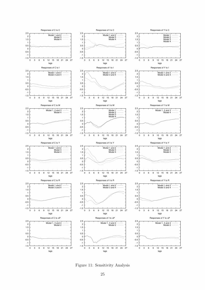
specifications output of the search procedure. I focus the sensitivity analysis on the models in

which interest rate precedes investment and output. I call model 2 the model which is equal

to model 1, except that the relation between real balances and inflation is inverted (we have

M ← ∆P ), I call model 3 the model, which corresponds to graph (ii) of Figure 4 and I call

23

-1.5-1

-0.50

0.51

1.52

2.5

0 3 6 9 12 15 18 21 24 27lags

Responses of C to DP

-1.5-1

-0.50

0.51

1.52

2.5

0 3 6 9 12 15 18 21 24 27lags

Responses of I to DP

-1.5-1

-0.50

0.51

1.52

2.5

0 3 6 9 12 15 18 21 24 27lags

Responses of Y to DP

Figure 10: Responses of consumption, investment, and output to one-standard-deviation shock

in inflation

model 4 which is equal to model 3, except that the relation between real balances and inflation

is M ← ∆P . Figure 11 shows the impulse response functions calculated for the four models.

There are no relevant differences between the impulse response functions derived by model 1

and 2, except for minor differences in the response of I to the real balance shock and in the

responses of C, I and Y to the inflation shock.

The impulse response functions calculated using model 3 present some relevant differences

with respect to the response functions calculated using the other models. The responses of

C to I using model 3 have a shape similar to the responses using 1, except that the former

are much lower than the latter: model 3 yields responses of C to I negative in the long-run.

The same evidence holds for the responses of Y to I. These differences make model 1 more

consistent with broadly accepted stylized facts. There are also quantitative differences as far

as responses of I to Y and R are concerned. In particular the responses of I to R are negative

for the first three years.

Model 4 yields responses which also present some important differences with respect to the

other models. The shape of the responses of I and Y to consumption shocks are quite different

from the shape of the responses derived from the other models. The responses of C to output

shock are almost null (while in the other models result slightly positive), the responses of I

and Y to output shock are also mostly below the other responses. In the other cases, the

responses of model 4 are very similar to the responses of model 3.

The results presented here confirm somewhat the analysis of King et al. (1991), according

to which postwar US macroeconomic data do not support the key implication of the standard

real business cycle model, that permanent productivity shocks are the dominant source of

economic fluctuations. Indeed monetary shocks and interest rate shocks seem to play a role

not inferior to the one played by shocks associated with consumption, investment and output.

The present analysis is different from the one of King et al. (1991), because these authors

24

-1.5-1

-0.5 0

0.5 1

1.5 2

2.5

27 24 21 18 15 12 9 6 3 0lags

Responses of C to C

Model 1 and 2Model 3Model 4

-1.5-1

-0.5 0

0.5 1

1.5 2

2.5

27 24 21 18 15 12 9 6 3 0lags

Responses of I to C

Model 1 and 2Model 3Model 4

-1.5-1

-0.5 0

0.5 1

1.5 2

2.5

27 24 21 18 15 12 9 6 3 0lags

Responses of Y to C

Model 1Model 2Model 3Model 4

-1.5-1

-0.5 0

0.5 1

1.5 2

2.5

27 24 21 18 15 12 9 6 3 0lags

Responses of C to I

Model 1 and 2Model 3 and 4

-1.5-1

-0.5 0

0.5 1

1.5 2

2.5

27 24 21 18 15 12 9 6 3 0lags

Responses of I to I

Model 1 and 2Model 3 and 4

-1.5-1

-0.5 0

0.5 1

1.5 2

2.5

27 24 21 18 15 12 9 6 3 0lags

Responses of Y to I

Model 1 and 2Model 3 and 4

-1.5-1

-0.5 0

0.5 1

1.5 2

2.5

27 24 21 18 15 12 9 6 3 0lags

Responses of C to M

Model 1, 2 and 3Model 4

-1.5-1

-0.5 0

0.5 1

1.5 2

2.5

27 24 21 18 15 12 9 6 3 0lags

Responses of I to M

Model 1Model 2Model 3Model 4

-1.5-1

-0.5 0

0.5 1

1.5 2

2.5

27 24 21 18 15 12 9 6 3 0lags

Responses of Y to M

Model 1, 2 and 3Model 4

-1.5-1

-0.5 0

0.5 1

1.5 2

2.5

27 24 21 18 15 12 9 6 3 0lags

Responses of C to Y

Model 1 and 2Model 3Model 4

-1.5-1

-0.5 0

0.5 1

1.5 2

2.5

27 24 21 18 15 12 9 6 3 0lags

Responses of I to Y

Model 1 and 2Model 3Model 4

-1.5-1

-0.5 0

0.5 1

1.5 2

2.5

27 24 21 18 15 12 9 6 3 0lags

Responses of Y to Y

Model 1 and 2Model 3Model 4

-1.5-1

-0.5 0

0.5 1

1.5 2

2.5

27 24 21 18 15 12 9 6 3 0lags

Responses of C to R

Model 1 and 2Model 3 and 4

-1.5-1

-0.5 0

0.5 1

1.5 2

2.5

27 24 21 18 15 12 9 6 3 0lags

Responses of I to R

Model 1 and 2Model 3 and 4

-1.5-1

-0.5 0

0.5 1

1.5 2

2.5

27 24 21 18 15 12 9 6 3 0lags

Responses of Y to R

Model 1 and 2Model 3 and 4

-1.5-1

-0.5 0

0.5 1

1.5 2

2.5

27 24 21 18 15 12 9 6 3 0lags

Responses of C to ∆P

Model 1, 3 and 4Model 2

-1.5-1

-0.5 0

0.5 1

1.5 2

2.5

27 24 21 18 15 12 9 6 3 0lags

Responses of I to ∆P

Model 1, 3 and 4Model 2

-1.5-1

-0.5 0

0.5 1

1.5 2

2.5

27 24 21 18 15 12 9 6 3 0lags

Responses of Y to ∆P

Model 1, 3 and 4Model 2

Figure 11: Sensitivity Analysis

25

impose long-run restrictions in order to obtain three permanent shocks (associated with the

common stochastic trends) and three transitory shocks (associated with the cointegrating

relationships)7. In my analysis each of the six shocks (each of them associated with a particular

variable) has, at least theoretically, permanent effects. Thus, it is possible to distinguish

among the three real flow variables shocks. Among C, I and Y shocks, the shock associated

with investment seems to play the largest role in the short-run. In the long-run a larger role

is played by shocks associated with consumption and output. An interesting result of the

present analysis is the major role played by the monetary shock, as I interpret the shock

associated with M . In the medium-run the effect is non-monotonic, but the permanent effect

is largely positive. This result is consistent with the the claim that monetary shocks, not

only productivity shocks, are the sources of macroeconomic fluctuations. An important role

is also played by the shock associated with the interest rate. Here the responses are much

more fluctuating than the case of M shock: positive in the short-run, considerably negative

in the medium-run and positive in the long-run. The effect of this shock on investment is

particularly large in the short and in the long-run. Thus an important source of economic

fluctuations is associated with this shock, in accordance with the results of King et al. (1991).

But, as these authors point out, it is somewhat difficult to interpret this shock with standard

macroeconomic models. It is also confirmed the small role played by inflation on output in

the long-run. Although it has a larger role in explaining investment movements, this result

seems at odds with a monetarist perspective.8

The sensitivity analysis can be straightforwardly extended to the other 12 models in which

interest rate does not causally precede investment and output. I do not report these results

here, which do not change the substance of the main conclusions9. However, let us emphasize

that the main advantage of using this method consists in dealing with a reasonably limited

7For a criticism of the use of long-run restrictions to identify a VAR, see Faust and Leeper (1997).8It may also be useful to compare the impulse responses functions obtained in this analysis with the impulse

responses functions obtained by King et al. (1991). (See Figure 4 in King et al. (1991, p. 834)). In the six

variables model, these authors study the effect of three permanent shock: balanced-growth shock, inflation

shock, and real interest rate shock. The shape of the responses of C, I and Y to the balanced growth shock

does not present significant similarities with the responses to the consumption, investment or output shock of

the present analysis, except for the fact that the responses tend to be positive in both analyses. Perhaps in my

analysis it emerges even with more evidence the fact that shocks related to real variables are not significantly

more important than shocks related to nominal variables. The responses of Y and C to the inflation shock in

the analysis of King et al. are very similar to the responses obtained in my analysis, while the response of I to

the same shock is very different: mostly positive in the analysis of King et al, mostly negative in my analysis.

There also some similarities in the shape of the responses of C, I and Y to the real (nominal in my analysis)

interest shock between the analysis of King et al. and my analysis, but the responses are quite different in

quantitative terms.9Results on the other specifications are available from the author on request.

26

number of models in the sensitivity analysis. Furthermore, the class of models output of my

search procedure is a class of overidentified models that can be tested.

5 Conclusions

In this paper a method to identify the causal structure related to a VAR has been proposed.

Particular emphasis has been posed on the causal structure among contemporaneous vari-

ables, which explains the correlations and the partial correlations among the residuals. The

identification of the causal structure among the contemporaneous variables has permitted an

orthogonalization of the residuals, which is alternative to the common practice, which uses the

Choleski factorization and has been often criticized as arbitrary. The method of identification

proposed is based on a graphical search algorithm, which has as inputs tests on vanishing

partial correlations among the residuals. Although the method is apparently data-driven,

the more background knowledge is incorporated, the more detailed is the causal structure

identified. Also the reliability of the latter depends on the reliability of the former. One of

the claimed advantage of this method is to give to background knowledge an explicit causal

form. In the empirical example considered, prior economic knowledge was essential to select

the appropriate model, but since the number of acceptable models was reasonably low, it was

possible to assess the robustness of the results to different causal restrictions.

This method will result much improved if the possibility of latent variables and the pos-

sibility of feedbacks and cycles (among contemporaneous variables) will be taken into con-

sideration. Such possibilities should be addressed jointly with the problem of aggregation.

Directions for further research may consider these issues.

Appendix A: Testing vanishing partial correlations among

residuals

In this appendix I provide a procedure to test the null hypotheses of vanishing correlations

and vanishing partial correlations among the residuals. Tests are based on asymptotic results.

Let us write the VAR which is estimated in a more compact form, denoting X ′t = [Y ′t−1,

...,Y ′t−p], which has dimension (1× kp) and Π′ = [A1, . . . , Ap], which has dimension (k × kp).It is possible to write: Yt = Π′Xt + ut. The maximum likelihood estimate of Π turns out to

be given by

Π′ =

[T∑

t=1

YtX′t

][T∑

t=1

XtX′t

]−1

.

27

Moreover, the ith row of Π′ is

π′i =

[T∑

t=1

yitX′t

][T∑

t=1

XtX′t

]−1

,

which coincides with the estimated coefficient vector from an OLS regression of yit on Xt

(Hamilton 1994, p. 293). The maximum likelihood estimate of the matrix of variance and co-

variance among the error terms Σu turns out to be Σu = (1/T )∑T

t=1 utu′t, where ut = Yt−Π′Xt.

Therefore the maximum likelihood estimate of the covariance between uit and ujt is given by

the (i, j) element of Σu: σij = (1/T )∑T

t=1 uitujt.

Proposition A.1 (Hamilton 1994, p. 301). Let Yt = A1Yt−1 + A2Yt−2 + . . . + ApYt−p + ut

where ut ∼ i.i.d. N(0,Σu) and where roots of |Ik − A1z − A2z2 − . . .− Apzp| = 0 lie outside

the unit circle. Let Σu be the maximum likelihood estimate of Σu. Then

√T [vech(Σu)− vech(Σu)]

d−→ N(0, Ω), (12)

where Ω = 2D+k (Σu ⊗ Σu)(D+

k )′, D+′k ≡ (D′kDk)

−1D′k and Dk is the duplication matrix.

Therefore, to test the null hypothesis that ρ(uit, ujt) = 0, I use the Wald statistic:

T (σij)2

σiiσjj + σ2ij

≈ χ2(1).

The Wald statistic for testing vanishing partial correlations is obtained by means of the delta

method.

Proposition A.2 (delta method, see e.g. Lehmann-Casella, 1998, p. 61). Let XT be

a (r × 1) sequence of vector-valued random-variables (indexed by the sample size T ). If

[√T (X1T − θ1), . . . ,

√T (XrT − θr)]

d−→ N(0,Σ) and h1, . . . , hr are r real-valued functions

of θ = (θ1, . . . , θr), hi : Rr → R, defined and continuously differentiable in a neighborhood

ω of the parameter point θ and such that the matrix B = ||∂hi/∂θj|| of partial derivatives is

nonsingular in ω, then:

[√T [h1(XT )− h1(θ)], . . . ,

√T [hr(XT )− hr(θ)]] d−→ N(0, BΣB′).

For example, for k = 4, suppose one wants to test ρ(u1, u3|u2) = 0. First, notice that

ρ(u1, u3|u2) = 0 if and only if σ22σ13 − σ12σ23 = 0 (see definition of partial correlation in

Anderson 1958, p. 34), where σij is the (i, j) element of Σu. Let us define a function g :

Rk(k+1)/2 → R, such that g(vech(Σu)) = σ22σ13 − σ12σ23. Thus,

∇g′ = (0, −σ23, σ22, 0, σ13, −σ12, 0, 0, 0, 0).

28

Proposition A.2 implies that:

√T [(σ22σ13 − σ12σ23) − (σ22σ13 − σ12σ23)]

d−→ N(0,∇g′Ω∇g).

The Wald test of the null hypothesis ρ(u1, u3|u2) = 0 is given by:

T (σ22σ13 − σ12σ23)2

∇g′Ω∇g ≈ χ2(1).

Suppose now I want to test the null hypothesis ρ(u1, u4|u2, u3) = 0, which implies σ22σ33σ14−σ33σ12σ24−σ14σ

223−σ22σ13σ34 +σ13σ23σ24 +σ12σ23σ34 = 0. I define g(vech(Σu)) = σ22σ33σ14−

σ33σ12σ24 − σ14σ223 − σ22σ13σ34 + σ13σ23σ24 + σ12σ23σ34. Thus,

∇g =

0

−σ33σ24 + σ23σ34

−σ22σ34 + σ23σ24

σ22σ33 − σ223

σ33σ14 − σ13σ34

−2σ14σ23 + σ13σ24 + σ12σ34

−σ12σ33 + σ13σ23

σ22σ14 − σ12σ24

−σ22σ13 + σ12σ23

0

.

Let us call τ14.23=(σ22σ33σ14 − σ33σ12σ24 − σ14σ223 − σ22σ13σ34 + σ13σ23σ24 + σ12σ23σ34) and

τ14.23 = (σ22σ33σ14 − σ33σ12σ24 − σ14σ223 − σ22σ13σ34 + σ13σ23σ24 + σ12σ23σ34). Proposition A.2

implies that: √T [τ14.23 − τ14.23]

d−→ N(0,∇g′Ω∇g).

The Wald test of the null hypothesis ρ(u1, u4|u2, u3) = 0 is given by:

T (τ14.23)2

∇g′Ω∇g ≈ χ2(1).

Tests for higher order correlations follow analogously.

Appendix B: Proof of Proposition 3.2

(i) Suppose yit and yjt are d-separated by Jt−1 and Yt in G. If there is a path in G between

yit and yjt that contains only components of Yt (and possibly of ut), such path is not active.

Then any path in GYt between yit and yjt is not active. Then yit and yjt are d-separated by

Yt in GYt.(ii) Suppose yit and yjt are d-separated by Yt in GYt . Then, if there is an active path between

29

yit and yjt in G, such path must contain a component of Jt−1 which is not a collider, since there

are no directed edge from any component of Yt pointing to any component of Jt−1. Therefore

such path is not active relative to Jt−1 in G and yit and yjt are d-separated by Jt−1 and Yt in

G.

References

Aldrich, J., 1989, Autonomy, Oxford Economic Papers, 41, 15-34.

Anderson, T.W., 1958, An Introduction to Multivariate Statistical Analysis, New York: Wiley.

Awokuse, T.O., and D.A. Bessler, 2003, Vector Autoregressions, Policy Analysis, and Directed

Acyclic Graphs: an Application to the U.S. Economy, Journal of Applied Economics, 6 (1),

1-24.

Bernanke, B.S., 1986, Alternative Explanations of the Money-Income Correlation, Carnegie-

Rochester Conference Series on Public Policy, 25, 49-100.

Bessler, D.A., and S. Lee, 2002, Money and prices: US data 1869-1914 (a study with directed

graphs), Empirical Economics, 27 (3), 427-446.

Bessler, D.A., and J. Yang, 2003, The Structure of Interdependence in International Stock

Markets, Journal of International Money and Finance, 22 (2), 261-287.

Blalock, H., 1971, Causal Models in the Social Sciences, Chicago: Aldine-Atherton.

Dahlhaus R., and M. Eichler, 2000, Causality and Graphical Models for Time Series, in P.

Green, N. Hjort, and S. Richardson (eds.), Highly Structured Stochastic Systems, Oxford:

Oxford University Press.

Demiralp, S. and K.D. Hoover, 2003, Searching for the Causal Structure of a Vector Autore-

gression, Oxford Bulletin of Economics and Statistics, 65, 745-767.

Doan, T.A., 2000, RATS Version 5, User’s Guide, Evanston, IL: Estima.

Faust, J. and E.M. Leeper, 1997, When Do Long-Run Identifying Restrictions Give Reliable

Results?, Journal of Business and Economic Statistics, 15 (3), 345-353.

Gibbs, W., 1902, Elementary Principles of Statistical Mechanics, New Haven: Yale University

Press.

Gilli, M., 1992, Causal Ordering and Beyond, International Economic Review, 33 (4), 957-971.

30

Glymour, C. and P. Spirtes, 1988, Latent Variables, Causal Models and Overidentifying Con-

straints, Journal of Econometrics, 39 (1), 175-198.

Granger, C.W.J., 1988, Some recent developments in a concept of causality, Journal of Econo-

metrics, 39 (1), 199-211.

Haigh, M., and D.A. Bessler, 2004, Causality and Price Discovery: An Application of Directed

Acyclic Graphs, Journal of Business, 77 (4), 1099-1121.

Hamilton, J., 1994, Time Series Analysis, Princeton: Princeton University Press.

Hausman, D.M. and J. Woodward, 1999, Independence, Invariance and the Causal Markov

Condition, British Journal of Philosophy of Science, 50, 521-583.

Hoover, K.D., 2001, Causality in Macroeconomics, Cambridge: Cambridge University Press.

Johansen, S., 1988, Statistical Analysis of Cointegrating Vectors, Journal of Economic Dy-

namics and Control, 12, 231-254.

Johansen, S., 1991, Estimation and hypothesis testing of cointegrating vectors in Gaussian

vector autoregressive models, Econometrica, 59 (6), 1551-1580.

King, R.G., C.I. Plosser, J.H. Stock, and M.W. Watson, 1991, Stochastic trends and economic

fluctuations, The American Economic Review, 81(4), 819-840.

Lauritzen, S.L., 1995, Graphical Models, Oxford: Clarendon Press.

Lauritzen, S.L., 2001, Causal inference from graphical models, in: E. Barndorff-Nielsen, D.R.

Cox, and C. Kluppelberg, eds., Complex Stochastic Systems, London: CRC Press.

Lehmann, E. L. and G. Casella, 1998, Theory of point estimation, New York: Springer Verlag.

Lutkepohl, H., 1991, Introduction to Multiple Time Series Analysis, Berlin and Heidelberg:

Springer Verlag.

Moneta, A., 2004, Identification of Monetary Policy Shocks: A Graphical Causal Approach,

Notas Economicas, 20.

Pearl, J., 1988, Probabilistic Reasoning in Intelligent Systems, San Francisco: Morgan Kauf-

mann.

Pearl, J., 2000, Causality: Models, Reasoning and Inference. Cambridge: Cambridge Univer-

sity Press.

31

Reale, M., and G. Tunnicliffe Wilson, 2001, Identification of vector AR models with recursive

structural errors using conditional independence graphs, Statistical Methods and Applica-

tions, 10 (1), 49-65.

Richardson, T. and P. Spirtes, 1999, Automated Discovery of Linear Feedback Models, in: C.

Glymour and G.F. Cooper, eds., Computation, Causation and Discovery, Menlo Park, CA:

AAAI Press and The MIT Press.

Scheines, R., P. Spirtes, C. Glymour and C. Meek, 1994, TETRAD 2: User’s Manual and

Software, New Jersey: Lawrence Erlbaum Associates, Inc.

Simon, H., 1953, Causal ordering and identifiability, in: W.C. Hood and T.C. Koopmans, eds.,

Studies in Econometric Methods, pp. 49-74. New York: Wiley.

Sims, C.A., 1980, Macroeconomics and Reality, Econometrica, 48, 1-47.

Spirtes, P., C. Glymour and R. Scheines, 2000, Causation, Prediction, and Search, 2nd edn,

Cambridge MA: The MIT Press.

Spirtes, P., R. Scheines, C. Meek, T. Richardson, C. Glymour, H. Hoi-

jtink and A. Boomsma (1996) TETRAD 3: Tools for Causal Modeling, at

http://www.phil.cmu.edu/tetrad/tet3/master.htm.

Swanson, N.R. and C.W.J. Granger, 1997, Impulse Response Function Based on a Causal

Approach to Residual Orthogonalization in Vector Autoregressions, Journal of the American

Statistical Association, 92(437), 357-367.

Verma, T., and J. Pearl, 1990, Equivalence and synthesis of causal models, Proceedings of the

Sixth Conference on Uncertainty in AI, Mountain View CA: Association for Uncertainty in

AI.

Whittaker, J., 1990, Graphical models in applied multivariate statistics, Chichester: Wiley.

Wold, H.O.A., 1954, Causality and econometrics, Econometrica, 62 (2), 162-177.

Wright, S., 1921, Correlation and causation, Journal of Agricultural Research, 20, 557-585.

Wright, S., 1934, The Method of Path Coefficients, Annals of Mathematical Statistics, 5 (3),

161-215.

Zellner, A., 1962, An Efficient Method of Estimating Seemingly Unrelated Regressions and

Tests for Aggregation Bias, Journal of the American Statistical Association, 57 (298), 348-

368.

32