Graphical Data and Data Graphics - Department of …paul/Talks/gddgVienna.pdf · Paul Murrell...

Paul Murrell Graphical Data and Data Graphics

Graphical Data and Data Graphics

Paul Murrell

The University of Auckland

July 12 2007


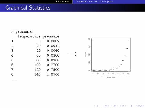
Graphical Statistics

> pressuretemperature pressure

1 0 0.00022 20 0.00123 40 0.00604 60 0.03005 80 0.09006 100 0.27007 120 0.75008 140 1.8500...

→● ● ● ● ● ● ● ● ● ● ●

●●

●

●

●

●

●

●

0 50 100 150 200 250 300 350

020

040

060

080

0

temperature

pres

sure


Statistical Graphics

> pressuretemperature pressure

1 0 0.00022 20 0.00123 40 0.00604 60 0.03005 80 0.09006 100 0.27007 120 0.75008 140 1.8500...

→● ● ● ● ● ● ● ● ● ● ●

●●

●

●

●

●

●

●

temperature

pres

sure

0 50 100 150 200 250 300 350

020

040

060

080

0


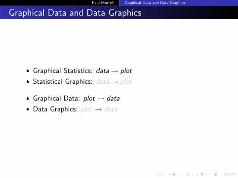
Graphical Data and Data Graphics

� Graphical Statistics: data→ plot

� Statistical Graphics: data→ plot

� Graphical Data: plot → data

� Data Graphics: plot → data


Graphical Formats

Raster

pixmap packageEBimage package

Vector

1

2 3

4 56

7 8

910

1112

1314

1516

1

2 3 45

67

grImport package


The grImport Package

PostScript[file]

PostScriptTrace()

ghostscript

RGML[file]

readPicture() "Picture"[R object]

grid.picture()

grid.symbols()


The PostScript Bezier Tiger

%!PS-Adobe-2.0 EPSF-1.2

%%Creator: Adobe Illustrator(TM)

%%For: OpenWindows Version 2

%%Title: tiger.eps

...

.8 setgray

clippath fill

-110 -300 translate

1.1 dup scale

0 g

0 G

0 i

0 J

0 j

0.172 w

10 M

[]0 d

0 0 0 0 k

...


Converting the Tiger to Data

PostScriptTrace("tiger.ps")

tiger <-readPicture("tiger.ps.xml")


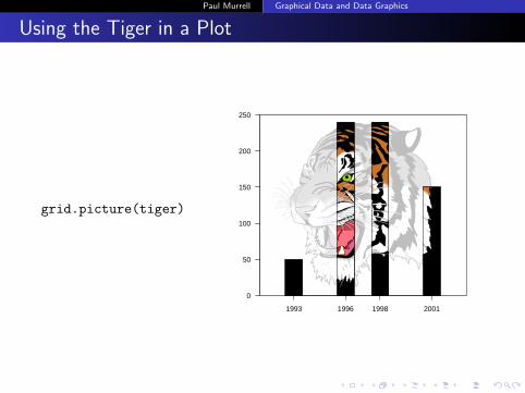
Using the Tiger in a Plot

grid.picture(tiger)

1993 1996 1998 2001

0

50

100

150

200

250

Estimated Population (max.) of Bengal Tigers(in Bhutan)

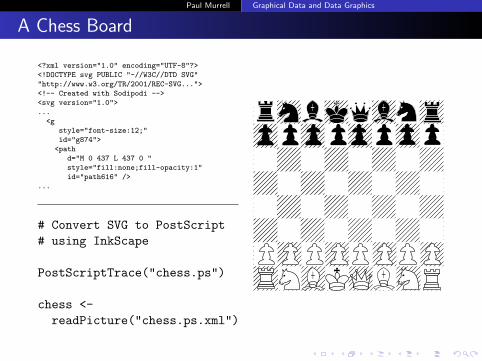
A Chess Board

<?xml version="1.0" encoding="UTF-8"?>

<!DOCTYPE svg PUBLIC "-//W3C//DTD SVG"

"http://www.w3.org/TR/2001/REC-SVG...">



<svg version="1.0">

...

<g

style="font-size:12;"

id="g874">

<path

d="M 0 437 L 437 0 "

style="fill:none;fill-opacity:1"

id="path616" />

...

# Convert SVG to PostScript# using InkScape

PostScriptTrace("chess.ps")

chess <-readPicture("chess.ps.xml")


The Paths in the Chess Board

picturePaths(chess[125:136])

1 2 3

4 5 6

7 8 9

10 11 12


A Chess Piece as a Plotting Symbols

The number of moves required to complete chess games fordifferent opening gambits. From the career of Louis Charles MaheDe La Bourdonnais (circa 1830).

grid.symbols(chess[205:206],x=games$num.moves,y=1:ngames,"native",size=unit(0.5, "cm"))

20 40 60 80

07 C51 Evans Gambit

Match C51 Evans Gambit

London m 18 C33 King's Gambit Accepted

03 D20 Queen's Gambit Accepted

London B21 Sicilian, 2.f4 and 2.d4

09 C38 King's Gambit Accepted

London A03 Bird's Opening

11 C51 Evans Gambit


London D20 Queen's Gambit Accepted

13 C51 Evans Gambit


03 C51 Evans Gambit

London C51 Evans Gambit



18 B30 Sicilian

07 C51 Evans Gambit

04 D20 Queen's Gambit Accepted

London C53 Giuoco Piano

06 B21 Sicilian, 2.f4 and 2.d4

London m1 C23 Bishop's Opening


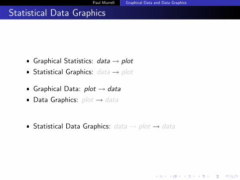
Statistical Data Graphics

� Graphical Statistics: data→ plot

� Statistical Graphics: data→ plot

� Graphical Data: plot → data

� Data Graphics: plot → data

� Statistical Data Graphics: data→ plot → data


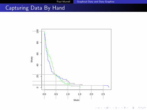
Capturing Data By Hand

0.0 0.5 1.0 1.5 2.0 2.5

020

4060

8010

0

bluex

blue

y


Capturing Data By Hand


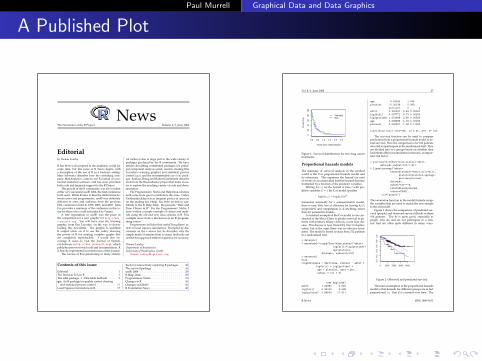
A Published Plot

NewsThe Newsletter of the R Project Volume 4/1, June 2004

Editorialby Thomas Lumley

R has been well accepted in the academic world forsome time, but this issue of R News begins witha description of the use of R in a business setting.Marc Schwartz describes how his consulting com-pany, MedAnalytics, came to use R instead of com-mercial statistical software, and has since providedboth code and financial support to the R Project.

The growth of the R community was also evidentat the very successful useR! 2004, the first conferencefor R users. While R aims to blur the distinctions be-tween users and programmers, useR! was definitelydifferent in aims and audience from the previousDSC conferences held in 1999, 2001, and 2003. JohnFox provides a summary of the conference in this is-sue for those who could not make it to Vienna.

A free registration to useR! was the prize inthe competition for a new graphic for http://www.

r-project.org. You will have seen the winninggraphic, from Eric Lecoutre, on the way to down-loading this newsletter. The graphic is uneditedR output (click on it to see the code), showingthe power of R for creating complex graphs thatare completely reproducible. I would also en-courage R users to visit the Journal of Statisti-cal Software (http:///www.jstatsoft.org), whichpublishes peer-reviewed code and documentation. Ris heavily represented in recent issues of the journal.

The success of R in penetrating so many statisti-

cal niches is due in large part to the wide variety ofpackages produced by the R community. We havearticles describing contributed packages for princi-pal component analysis (ade4, used in creating EricLecoutre’s winning graphic) and statistical processcontrol (qcc) and the recommended survival pack-age. Jianhua Zhang and Robert Gentlement describetools from the Bioconductor project that make it eas-ier to explore the resulting variety of code and docu-mentation.

The Programmers’ Niche and Help Desk columnsboth come from guest contributors this time. GaborGrothendieck,known as frequent poster of answerson the mailing list r-help, has been invited to con-tribute to the R Help Desk. He presents “Date andTime Classes in R”. For the Programmers’ Niche, Ihave written a simple example of classes and meth-ods using the old and new class systems in R. Thisexample arose from a discussion at an R program-ming course.

Programmers will also find useful Doug Bates’ ar-ticle on least squares calculations. Prompted by dis-cussions on the r-devel list, he describes why thesimple matrix formulae from so many textbooks arenot the best approach either for speed or for accuracy.

Thomas LumleyDepartment of BiostatisticsUniversity of Washington, Seattle

[email protected]

Contents of this issue:

Editorial . . . . . . . . . . . . . . . . . . . . . . 1The Decision To Use R . . . . . . . . . . . . . . 2The ade4 package - I : One-table methods . . . 5qcc: An R package for quality control charting

and statistical process control . . . . . . . . . 11Least Squares Calculations in R . . . . . . . . . 17

Tools for interactively exploring R packages . . 20The survival package . . . . . . . . . . . . . . . 26useR! 2004 . . . . . . . . . . . . . . . . . . . . . 28R Help Desk . . . . . . . . . . . . . . . . . . . . 29Programmers’ Niche . . . . . . . . . . . . . . . 33Changes in R . . . . . . . . . . . . . . . . . . . . 36Changes on CRAN . . . . . . . . . . . . . . . . 41R Foundation News . . . . . . . . . . . . . . . . 46

Vol. 4/1, June 2004 27

0.0 0.5 1.0 1.5 2.0 2.5

020

4060

8010

0

Years since randomisation

% s

urvi

ving

StandardNew

Figure 1: Survival distributions for two lung cancertreatments

Proportional hazards models

The mainstay of survival analysis in the medicalworld is the Cox proportional hazards model andits extensions. This expresses the hazard (or rate)of events as an unspecified baseline hazard functionmultiplied by a function of the predictor variables.

Writing h(t; z) for the hazard at time t with pre-dictor variables Z = z the Cox model specifies

log h(t, z) = log h0(t)eβz.

Somewhat unusually for a semiparametric model,there is very little loss of efficiency by leaving h0(t)unspecified, and computation is, if anything, easierthan for parametric models.

A standard example of the Cox model is one con-structed at the Mayo Clinic to predict survival in pa-tients with primary biliary cirrhosis, a rare liver dis-ease. This disease is now treated by liver transplan-tation, but at the same there was no effective treat-ment. The model is based on data from 312 patientsin a randomised trial.

> data(pbc)

> mayomodel<-coxph(Surv(time,status)~edtrt+

log(bili)+log(protime)+

age+platelet,

data=pbc, subset=trt>0)

> mayomodel

Call:

coxph(formula = Surv(time, status) ~ edtrt +

log(bili) + log(protime) +

age + platelet, data = pbc,

subset = trt > 0)

coef exp(coef)

edtrt 1.02980 2.800

log(bili) 0.95100 2.588

log(protime) 2.88544 17.911

age 0.03544 1.036

platelet -0.00128 0.999

se(coef) z p

edtrt 0.300321 3.43 0.00061

log(bili) 0.097771 9.73 0.00000

log(protime) 1.031908 2.80 0.00520

age 0.008489 4.18 0.00003

platelet 0.000927 -1.38 0.17000

Likelihood ratio test=185 on 5 df, p=0 n= 312

The survexp function can be used to comparepredictions from a proportional hazards model to ac-tual survival. Here the comparison is for 106 patientswho did not participate in the randomised trial. Theyare divided into two groups based on whether theyhad edema (fluid accumulation in tissues), an impor-tant risk factor.

> plot(survfit(Surv(time,status)~edtrt,

data=pbc,subset=trt==-9))

> lines(survexp(~edtrt+

ratetable(edtrt=edtrt,bili=bili,

platelet=platelet,age=age,

protime=protime),

data=pbc,

subset=trt==-9,

ratetable=mayomodel,

cohort=TRUE),

col="purple")

The ratetable function in the model formula wrapsthe variables that are used to match the new sampleto the old model.

Figure 2 shows the comparison of predicted sur-vival (purple) and observed survival (black) in these106 patients. The fit is quite good, especially aspeople who do and do not participate in a clin-ical trial are often quite different in many ways.

0 1000 2000 3000 4000

0.0

0.2

0.4

0.6

0.8

1.0

Figure 2: Observed and predicted survival

The main assumption of the proportional hazardsmodel is that hazards for different groups are in factproportional, i.e. that β is constant over time. The

R News ISSN 1609-3631


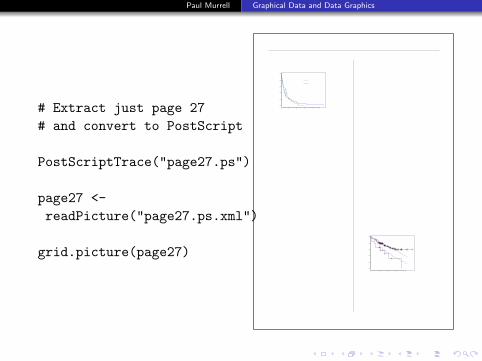
# Extract just page 27# and convert to PostScript

PostScriptTrace("page27.ps")

page27 <-readPicture("page27.ps.xml")

grid.picture(page27)


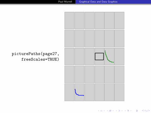
picturePaths(page27,freeScales=TRUE)


> grid.picture(page27[c(3:16, 17, 26)], gp=gpar(lex=.3))


> picturePaths(page27[c(3:16, 17, 26)])

3 4 5 6

7 8 9 10

11 12 13 14

15 16 17 18


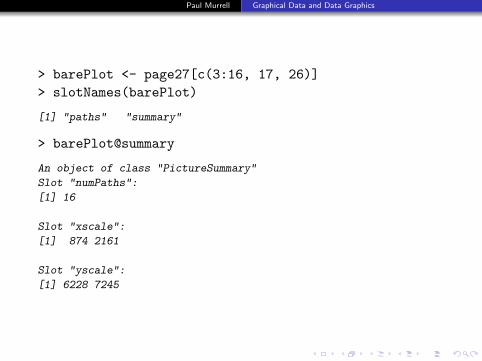
> barePlot <- page27[c(3:16, 17, 26)]> slotNames(barePlot)

[1] "paths" "summary"

> barePlot@summary

An object of class "PictureSummary"

Slot "numPaths":

[1] 16

Slot "xscale":

[1] 874 2161

Slot "yscale":

[1] 6228 7245


> class(barePlot@paths)

[1] "list"

> barePlot@paths[[1]]

An object of class "PictureStroke"

Slot "x":

move line

919 919

Slot "y":

move line

6273 6228

Slot "rgb":

[1] "#000000"

Slot "lwd":

[1] 6.23

Paul Murrell Graphical Data and Data GraphicsVol. 4/1, June 2004 27

0.0 0.5 1.0 1.5 2.0 2.5

020

4060

8010

0

Years since randomisation

% s

urvi

ving

StandardNew

Figure 1: Survival distributions for two lung cancertreatments

Proportional hazards models

The mainstay of survival analysis in the medicalworld is the Cox proportional hazards model andits extensions. This expresses the hazard (or rate)of events as an unspecified baseline hazard functionmultiplied by a function of the predictor variables.

Writing h(t; z) for the hazard at time t with pre-dictor variables Z = z the Cox model specifies

log h(t, z) = log h0(t)eβz.

Somewhat unusually for a semiparametric model,there is very little loss of efficiency by leaving h0(t)unspecified, and computation is, if anything, easierthan for parametric models.

A standard example of the Cox model is one con-structed at the Mayo Clinic to predict survival in pa-tients with primary biliary cirrhosis, a rare liver dis-ease. This disease is now treated by liver transplan-tation, but at the same there was no effective treat-ment. The model is based on data from 312 patientsin a randomised trial.

> data(pbc)

> mayomodel<-coxph(Surv(time,status)~edtrt+

log(bili)+log(protime)+

age+platelet,

data=pbc, subset=trt>0)

> mayomodel

Call:

coxph(formula = Surv(time, status) ~ edtrt +

log(bili) + log(protime) +

age + platelet, data = pbc,

subset = trt > 0)

coef exp(coef)

edtrt 1.02980 2.800

log(bili) 0.95100 2.588

log(protime) 2.88544 17.911

age 0.03544 1.036

platelet -0.00128 0.999

se(coef) z p

edtrt 0.300321 3.43 0.00061

log(bili) 0.097771 9.73 0.00000

log(protime) 1.031908 2.80 0.00520

age 0.008489 4.18 0.00003

platelet 0.000927 -1.38 0.17000

Likelihood ratio test=185 on 5 df, p=0 n= 312

The survexp function can be used to comparepredictions from a proportional hazards model to ac-tual survival. Here the comparison is for 106 patientswho did not participate in the randomised trial. Theyare divided into two groups based on whether theyhad edema (fluid accumulation in tissues), an impor-tant risk factor.

> plot(survfit(Surv(time,status)~edtrt,

data=pbc,subset=trt==-9))

> lines(survexp(~edtrt+

ratetable(edtrt=edtrt,bili=bili,

platelet=platelet,age=age,

protime=protime),

data=pbc,

subset=trt==-9,

ratetable=mayomodel,

cohort=TRUE),

col="purple")

The ratetable function in the model formula wrapsthe variables that are used to match the new sampleto the old model.

Figure 2 shows the comparison of predicted sur-vival (purple) and observed survival (black) in these106 patients. The fit is quite good, especially aspeople who do and do not participate in a clin-ical trial are often quite different in many ways.

0 1000 2000 3000 4000

0.0

0.2

0.4

0.6

0.8

1.0

Figure 2: Observed and predicted survival

The main assumption of the proportional hazardsmodel is that hazards for different groups are in factproportional, i.e. that β is constant over time. The

R News ISSN 1609-3631


3 4 5 6

7 8 9 10

11 12 13 14

15 16 17 18


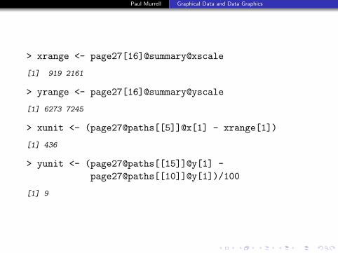
> xrange <- page27[16]@summary@xscale

[1] 919 2161

> yrange <- page27[16]@summary@yscale

[1] 6273 7245

> xunit <- (page27@paths[[5]]@x[1] - xrange[1])

[1] 436

> yunit <- (page27@paths[[15]]@y[1] -page27@paths[[10]]@y[1])/100

[1] 9


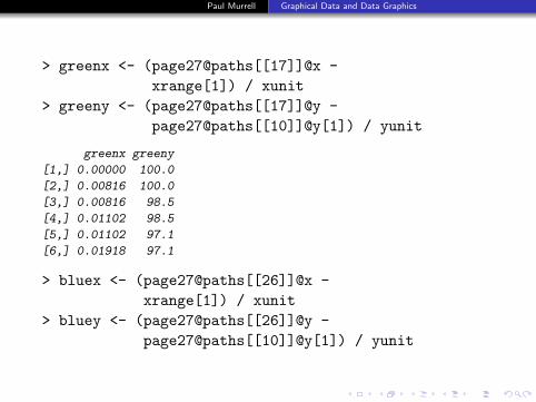
> greenx <- (page27@paths[[17]]@x -xrange[1]) / xunit

> greeny <- (page27@paths[[17]]@y -page27@paths[[10]]@y[1]) / yunit

greenx greeny

[1,] 0.00000 100.0

[2,] 0.00816 100.0

[3,] 0.00816 98.5

[4,] 0.01102 98.5

[5,] 0.01102 97.1

[6,] 0.01918 97.1

> bluex <- (page27@paths[[26]]@x -xrange[1]) / xunit

> bluey <- (page27@paths[[26]]@y -page27@paths[[10]]@y[1]) / yunit


> bluedupes <- duplicated(bluex)> bluecurve <- data.frame(x=bluex,

y=bluey)[!bluedupes, ]

x y

1 0.00000 100.0

2 0.00270 100.0

4 0.00543 97.1

6 0.01918 95.6

8 0.02188 92.6

10 0.03563 89.7

> greendupes <- duplicated(greenx)> greencurve <- data.frame(x=greenx,

y=greeny)[!greendupes, ]


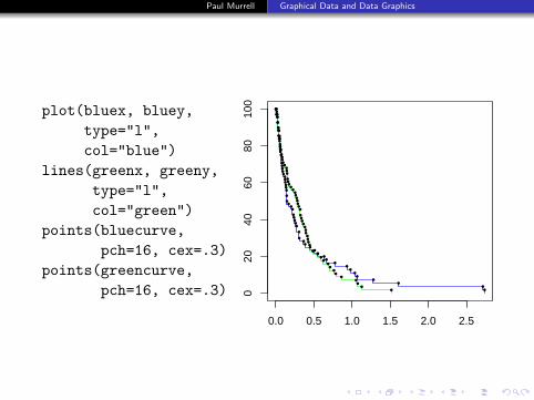
plot(bluex, bluey,type="l",col="blue")

lines(greenx, greeny,type="l",col="green")

points(bluecurve,pch=16, cex=.3)

points(greencurve,pch=16, cex=.3)

0.0 0.5 1.0 1.5 2.0 2.5

020

4060

8010

0

●●

●

●

●

●

●

●

●

●

●

●

●

●

●

●

●

●

●

●

●

●

●

●

●

●

●

●

●

●

●

●

●

●

●

●

●

●

●

●

●

●

●

●

●

●

●

●

●

●

●

●

●●

●

●

●

●

●

●

●

●

●

●

●

●

●

●

●

●

●

●

●

●

●

●

●

●

●

●

●

●

●

●

●

●

●

●

●

●

●

●

●

●

●

●

●

●

●

●

●

●

●

●

●

●

●

●

●

●


Problems

� Many articles, especially old ones where the plot is the onlydata available, contain bitmap images.

� Many articles, and their images, are fiercely guarded bydraconian copyright protections.

� Human intervention is still required.


Acknowledgements

� The tiger image is part of the ghostscript distribution; the tiger data are fromhttp://www.globaltiger.org/population.htm.

� The greyscale version of the tiger used the colorspace package by Ross Ihaka.

� The chess board image (by Jose Hevia) is from the Open Clip Art Libraryhttp://openclipart.org/clipart//recreation/games/chess/chess_game_01.svg

� The chess data are from chessgames.comhttp://www.chessgames.com/perl/chess.pl?page=1&pid=31596

� R News is a publication of the R Foundation for Statistical Computing. Thearticle used is The survival Package by Thomas Lumley R News, 4(1), pp.26–28.

� The application for measuring survival curves was suggested by Dan Jackson.

Graphical Data and Data Graphics - Department of …paul/Talks/gddgVienna.pdf · Paul Murrell...

Documents

Transcript of Graphical Data and Data Graphics - Department of …paul/Talks/gddgVienna.pdf · Paul Murrell...