Graphic Objects figure axes 2D-plot 3D-plot axis labels title GUI objects pushbutton toggle edit...

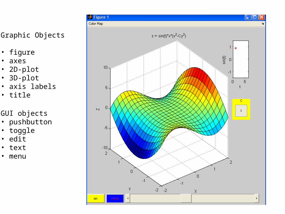
Graphic Objects

• figure• axes• 2D-plot• 3D-plot• axis labels• title

GUI objects• pushbutton• toggle• edit• text• menu

Continuing with our GUI project

Sliders

Sliders provide an easy way to gradually change values between a given range.

Three ways to move the slider

Sliders

The user has three possible way to change the position of the slider

1.Click the arrow buttons => small value changes

2.Click the trough => large value changes

3.Click and drag the slider => depends on user

The default changes are 1% and 10%

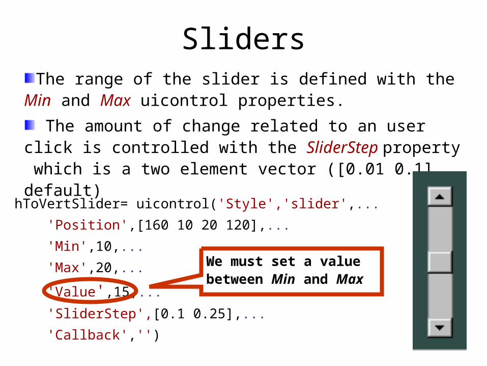
SlidersThe range of the slider is defined with the Min and

Max uicontrol properties.

The amount of change related to an user click is controlled with the SliderStep property which is a two element vector ([0.01 0.1] default)

hToVertSlider= uicontrol('Style','slider',...

'Position',[160 10 20 120],...

'Min',10,...

'Max',20,...

'Value',15,... 'SliderStep',[0.1 0.25],...

'Callback','')

We must set a value between Min and Max

Sliders

Given the setting from Min, Max and SliderStep the amount of change to the current Value are as follow:

For an arrow click:

Value = Value + SliderStep(1) * (Max – Min)

16 = 15 + 0.1 * (20 - 10)

For a trough click:

Value = Value + SliderStep(2) * (Max – Min)

17.5 = 15 + 0.25 * (20 - 10)

Step V– the speed slider

uicontrol('style' ,'slider',.... 'position',[130 10 450 30],... 'tag' ,'speedSlider',... 'max' ,pi/2,... 'min' ,0.01,... 'value' ,pi/4);

Step V– the speed slider

uicontrol('style' ,'slider',.... 'position',[130 10 450 30],... 'tag' ,'speedSlider',... 'max' ,pi/2,... 'min' ,0.01,... 'value' ,pi/4);

What about the callback?

Text and editable text Static texts are commonly used to give

instructions or to display other controllers values (such as sliders)

…’Style’,’text’,…

Static text can not execute callbacks.

Editable texts gets string input from the GUI user.

When the user enters the edit field and change its content, only the String property is affected.

Editable text can execute callbacks

Step VI – the text frame

uicontrol('style' ,'text',... 'string' ,'C',... 'tag' ,'C_title',... 'position' ,[490 290 60 70],... 'backgroundColor','y');

What about the callback?

Step VII – the edit window

uicontrol('style' ,'edit',... 'string' ,'1',... 'value' ,1,... 'tag' ,'C',... 'position',[500 300 40 40],... 'callback', {@getC});

function getC(calling_button, eventData) s = get(calling_button,'string'); set(calling_button,'value',str2double(s));end

Radio Buttons

Radio buttons are similar to checkboxes but designed to specify options that are mutually exclusive like in multiple-choice questions

hToRadio1 = uicontrol('Style', 'radio',...

'Position',[20 300 120 20],...

'String','Option1',...

'Callback', {@turnOffTheOtherButtons},...

'Value',1)

Selected

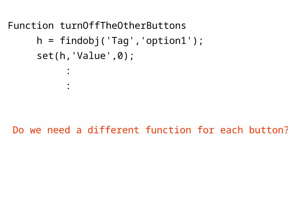
Function turnOffTheOtherButtons

h = findobj('Tag','option1');

set(h,'Value',0);

:

:

Do we need a different function for each button?

Step VIII – the radio buttons

uicontrol('style' ,'radio',... 'string' ,'surf',... 'callback', {@plotTypeButtons},... 'tag' ,'plot_type',... 'position',[490 250 80 30],... 'value' ,1,... 'userdata',1);

uicontrol('style' ,'radio',... 'string' ,'contour3',... 'callback', {@plotTypeButtons},... 'tag' ,'plot_type',... 'position',[490 220 80 30],... 'value' ,0,... 'userdata',0);

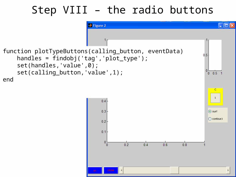
Step VIII – the radio buttons

function plotTypeButtons(calling_button, eventData) handles = findobj('tag','plot_type'); set(handles,'value',0); set(calling_button,'value',1);end

Step IX - Now lets use itfunction run(main_axes, small_axes) onOff = findobj('tag','onOff'); speedSlider = findobj('tag','speedSlider'); C_window = findobj('tag','C'); close_button = findobj('tag','close'); type_handels = findobj('tag','plot_type');

Step IX - Now lets use itfunction run(main_axes, small_axes) onOff = findobj('tag','onOff'); speedSlider = findobj('tag','speedSlider'); C_window = findobj('tag','C'); close_button = findobj('tag','close'); type_handles = findobj('tag','plot_type');

How does type_handles differ from the other handles?

kill = get(close_button,'userData'); [x y] = meshgrid(-2:0.2:2); t = 0.001; while (~kill) on = get(onOff,'userData'); C = get(C_window,'value'); speed = get(speedSlider,'value'); kill = get(close_button,'userData');

activeB = findobj(type_handels,'value',1); plotType = get(activeB,'userdata');

if (on) draw(x,y,main_axes,small_axes,t,C,plot_type); t = t + speed; if (t >= 2*pi) t = 0.0001; end end pause(0.1); end

kill = get(close_button,'userData'); [x y] = meshgrid(-2:0.2:2); t = 0.001; while (~kill) on = get(onOff,'userData'); C = get(C_window,'value'); speed = get(speedSlider,'value'); kill = get(close_button,'userData');

activeB = findobj(type_handels,'value',1); plotType = get(activeB,'userdata');

if (on) draw(x,y,main_axes,small_axes,t,C,plot_type); t = t + speed; if (t >= 2*pi) t = 0.0001; end end pause(0.1); end fig = findobj('tag','the_figure'); close(fig);end

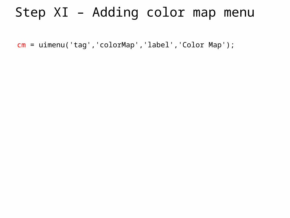
cm = uimenu('tag','colorMap','label','Color Map');

Step XI – Adding color map menu

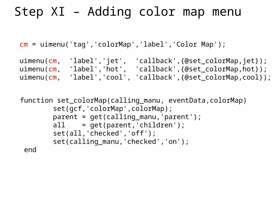
cm = uimenu('tag','colorMap','label','Color Map'); uimenu(cm, 'label','jet', ‘callback',{@set_colorMap,jet});uimenu(cm, 'label','hot', 'callback',{@set_colorMap,hot});uimenu(cm, 'label','cool', 'callback',{@set_colorMap,cool});

Step XI – Adding color map menu

function set_colorMap(calling_manu, eventData,colorMap) set(gcf,'colorMap',colorMap); parent = get(calling_manu,'parent'); all = get(parent,'children'); set(all,'checked','off'); set(calling_manu,'checked','on'); end

hToCheckBox =

uicontrol('Style', 'checkbox',...

'Position',[20 450 120 20],...

'String','Check Box example‘, ...

‘Callback’,’’)

Checkboxes allow the user to turn on/off a number of independent options

Note: the position is measured in pixels from the left-bottom corner of the figure

Checkboxes

26

Basics of Linear Algebra

start with two examples:

In 1st : We do not need Linear AlgebraIn 2nd : Linear Algebra is needed

27

Consider a species where N represents number of individuals. This species reproduces with a very simple rule: in any generation t (t = 0,1,2,....), the population changes its size by a factor of R.

Hence, at t+1 size of population isN(t+1) = R N(t).

Question: if we start with a population of size N(0), what will be its size after t generations?

28

gen=[1 2 3 4 5 6 7 8 9 10];

N0=100; %initial condition for populations

n1=N0; R1=1.1; %Params for population 1n2=N0; R2=0.9; %Params for population 2

for t=1:10 % numerical computation P1(t) = n1; n1 = n1*R1; %change pop 1 P2(t) = n2; n2 = n2*R2; %change pop 2 end

plot(gen,P1,'or:',gen,P2,'^b-');

Numerical computation (for two possible values of R)-

29

if R>1, the population grows to infinity. if R<1 it decays to 0.

P1

P2

30

In this case, there is an analytical solution

Back to Question: if we start with a population of size N(0), what will be its size after t generations?

In our case, the answer is trivial – no need for numerical computation:

For every t N(t+1) = RN(t)

Hence-N(t) = Rt N(0).

In our example-N1(10) = 1.110 * 100 = 2.59 *100 = 259 N2(10) = 0.910 * 100 = 0.35 *100 = 35

31

Simple problems have

analytical solutions

Complex problems can be solved only with

numerical computations

32

Reproduction-

1) age=0 (from birth to the age of 1) does not reproduce 2) age=1 yields 2 offsprings 3) age=2 yields 1.5 offsprings

Survival-

4) 40% of age 0 survive to next generation 5) 30% of age 1 survive to next generation6) 10% age 2 survive to next generation7) No females of age 3 survive.

For example, consider a species in which parameters are age-dependent.

33

Here the answer is more complex, because the system is defined by several equations, not only one:

Let Ni denote the number of individuals of age i.

N0(t+1) = 2N1(t)+1.5N2(t)N1(t+1) = 0.4N0(t)N2(t+1) = 0.3N1(t)N3(t+1) = 0.1N2(t)

N(t+1) = N0(t+1)+N1(t+1)+N2(t+1)+N3(t+1)

We may want to ask a questions like: what will be N(T)

We may want to ask additional questions like: when will the fraction of newborn stay constant, i.e:

Find t such that N0(t)/N(t) = N0(t+1)/N(t+1)?

34

To solve this problem, we need techniques from Linear Algebra.

Start by reviewing important concepts in Linear Algebra.

Will come back to this problem later, after learning some Linear Algebra

35

Matrix addition/substraction

Suppose A=[ai,j] and B=[bi,j] are two m x n matrices. ThenC=A+B is an m x n matrix where ci,j = ai,j+bi,j

for 1 im, 1j n

Example-

30

42

3011

1302

31

10

01

32

C

BA

36

Matrix addition/substraction

Example with 3 matrices-

60

41

330011

013102

30

01

31

10

01

32

CBA

CBA

37

Matrix Multiplication-

Suppose A=[ai,k] is an m by l matrix and B =[bk,j] is

an l by n matrix.

Then: C=A B is an m by n matrix with:

l

kkjikji bac

1,

mi 1

nj 1

In other words, in matrix C an element at place i,j is the result of multiplying the elements of row i in A by the elements of column j in B, and sum them up.

This is small L in Italics

38

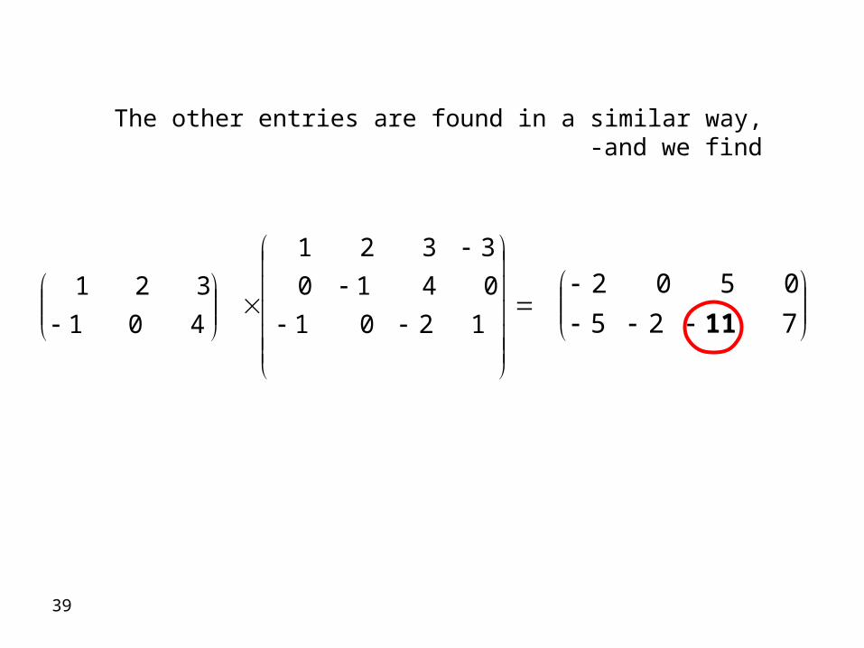
Example-

1201

0410

3321

401

321BA

BAC The multiplication is valid, because the number of columns in A is equal to the number of rows in B.

24232221

14131211

cccc

ccccC

The result is a matrix with 2 rows (number of rows in A) and 4 columns (number of columns in B).

To find any element cij, we multiply the elements of the ith row in A by the elements of the jth column of B, and sum them-

11803)2)(4()4)(0()3)(1(23 c

Second row elements in A

Third column elements in B

39

1201

0410

3321

401

321

The other entries are found in a similar way, and we find-

725

0502

11

40

In Matrix multiplication, the order is important ! in other words, AB BA:

Example:

112

0

1

1

AB

000

112

112

AB

41


Example:

112

0

1

1

AB

000

112

112

AB

42


Example where we reverse order of multiplication:

0

1

1

112 BA

000

112

112

AB

1)0)(1()1)(1()1)(2( BA

)from previous slide(

43

Check that you did it right


an l by n matrix.


l

kkjikji bac

1,

mi 1

nj 1

Test 1: Rows of first matrix = columns in second matrix

Test 1

44

Check that you did it right


an l by n matrix.


l

kkjikji bac

1,

mi 1

nj 1

Test 2

Test 1: Columns of first matrix = rows in second matrixTest 2: dimensions of resulting matrix are the rows of first and columns of second

45

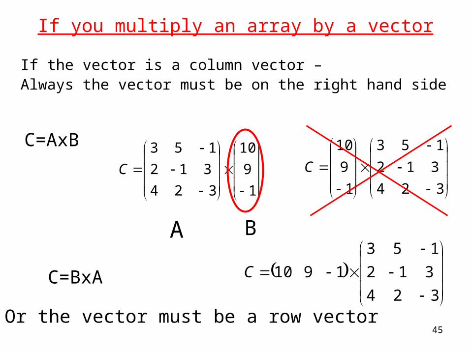
If you multiply an array by a vector

If the vector is a column vector – Always the vector must be on the right hand side

1

9

10

324

312

153

C

C=AxB

A B

324

312

153

1

9

10

C

324

312

153

1910C

Or the vector must be a row vector

C=BxA

46

Writing a system of linear equations in matrix form

nnnnnn

nn

nn

bxaxaxa

bxaxaxa

bxaxaxa

...

................................................

...

...

2211

22222121

11212111

Consider the following system of n equations with n variables xi, i=1..n.

It is convenient to represent this system of equations in matrix form:

nnnnnn

n

n

b

b

b

x

x

x

aaa

aaa

aaa

....

....

..............................

....

....

2

1

2

1

21

22221

11211

CoefficientMatrix

Vector of variables

Vector of Right Hand Side (RHS)Values

Matrix MultiplicationOperator

47

The system above can be also written in short :

bxA

CoefficientMatrix

Vector of variables

Vector of Right Hand Side (RHS)Values

Matrix MultiplicationOperator

bxA Or simply-

48

Power of Matrices

timesnAAA

AAA

n

..

2

Note- A must be a square matrix !!! Otherwise multiplication is undefined

So far – Linear Algebra. Let’s move back to MATLAB

49

Summary of what you know about Matrices in MatLab

1) A matrix is entered row-wise, with consecutive elements of a row separated by a space or a comma A=[ 1 2 3 ] A=[ 1, 2, 3 ]

2) Rows are separated by semicolons or carriage returns. B= [ 1 2 3 4 5 6 ]

3) Entire matrix must be enclosed within square brackets A=[ 1 2 3 ] 4) A single element of the matrix is accessed by specifying its index(ices), in round brackets. B(2,3)=6

5) Vector - a special case of a matrix. Can be column vector, or row vector

6) Scalar is a single element. It does not need brackets.

7) A null matrix is a matrix with no elements. It is defined by empty brackets []

50

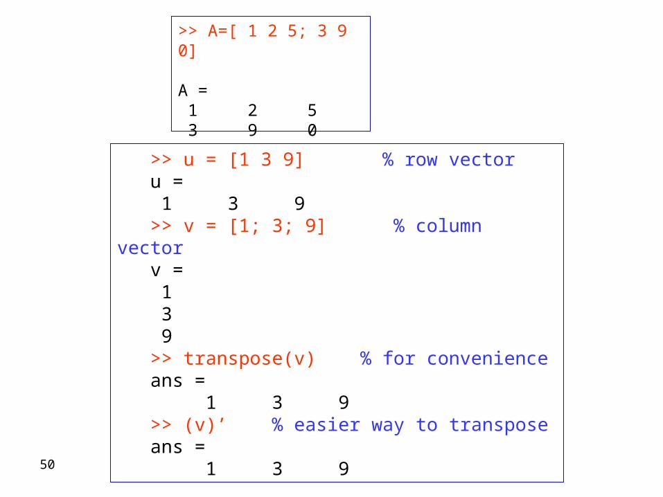
>> A=[ 1 2 5; 3 9 0]

A = 1 2 5 3 9 0

>> u = [1 3 9] % row vectoru = 1 3 9>> v = [1; 3; 9] % column vectorv = 1 3 9>> transpose(v) % for convenienceans = 1 3 9>> (v)’ % easier way to transposeans = 1 3 9

51

Matrix Transposition.

In this operation, rows and columns are interchanged:

654

321A

For example, if

Then-

6

5

4

3

2

1

'A

A convenient operation: When writing text, easier to write a column as row vector (takes less space).

52

>> A=[3 5 -1; 2 -1 3; 4 2 -3]; B=[1 2 3]

>> C=A*B??? Error using ==> *Inner matrix dimensions

must agree.

>> B=[1; 2; 3]>> C=A*B

>> (C)’ 10 9 -1

Matrix multiplication in MatLab-

Use the * operator to multiply matrices.Do NOT use the dot operation here (reserved for element by element)Make sure dimension are correct

53

The problem and its solutions

In a system with several linear equations Ax= b, given A and b, what is the vector of variables x ?

Three main Techniques:

1. Gaussian elimination and back-substitution2. The inverse matrix 3. Matrix division { related

1

9

10

324

312

153

3

2

1

x

x

xA b

54

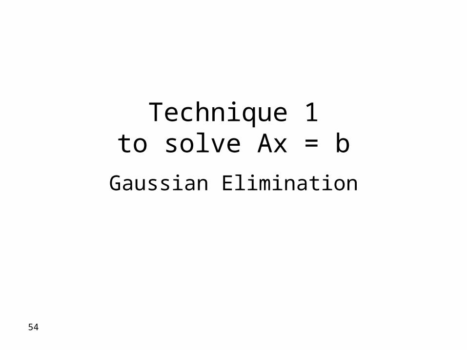
Technique 1to solve Ax = b

Gaussian Elimination

55

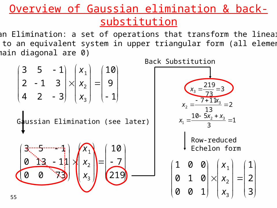
Overview of Gaussian elimination & back-substitution

1

9

10

324

312

153

3

2

1

x

x

x

219

7

10

7300

11130

153

3

2

1

x

x

x

Gaussian Elimination: a set of operations that transform the linear system to an equivalent system in upper triangular form (all elements below main diagonal are 0)

Gaussian Elimination (see later) 13

510

213

117

373

219

321

32

3

xxx

xx

x

Back Substitution

3

2

1

100

010

001

3

2

1

x

x

x

Row-reducedEchelon form

56

Needed for the Gaussian elimination:

Two basic operations can be used to transform a system oflinear equations into an equivalent system:

(1) Multiply an equation by a nonzero number(2) Adding one equation to the other

(we may need to use both operations)

Let’s remember some 8th grade algebra:

An equivalent system is a system of equations where thesolution is the same as the original system.

57

Example:

Eq. I: 3x + 2y = 8

Eq. II: 2x + 4y = 5

The solution of a system of several equations is found where the lines intersect

Solution

Multiplying Eq. I by +2, and Eq. II by -3 gives :Why did we choose these numbers? can get rid of x

Eq. I’: 6x + 4y = 16

Eq. II’: -6x - 12y = -15

Solution (where the lines intersect): same as before the operation

Solution

58

Replacing Eq. II’ by (Eq. I’+ Eq. II’) is like adding to Eq. II’ the other, Eq. I’ :

Eq. I’’: 6x + 4y = 16

Eq. II’’: -8y = 1

Solution (where the lines intersect): same as before operation

Solution

59

60

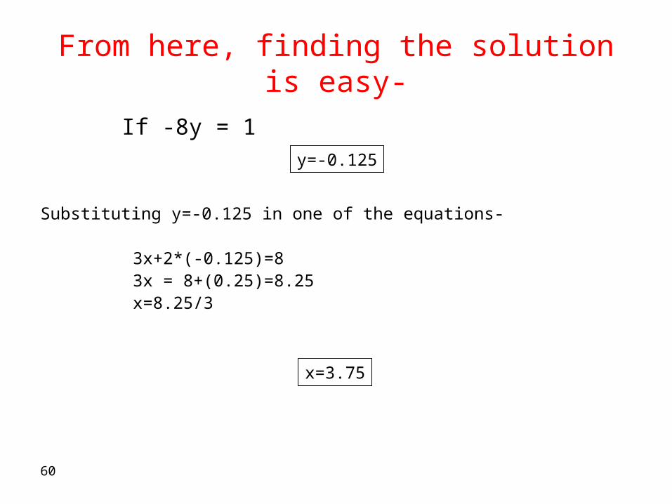
From here, finding the solution is easy-

If -8y = 1

Substituting y=-0.125 in one of the equations-

3x+2*(-0.125)=83x = 8+(0.25)=8.25x=8.25/3

y=-0.125

x=3.75

61

What did we do ?

3x + 2y = 8 Eq.I2x + 4y = 5 Eq. II

We multiplied Eq.I by +2 and Eq. II by -3:

6x + 4y = 16 Eq.I’ = Eq.I x 2-6x + -12y = -15 Eq. II’ = Eq. II x -3

We replaced Eq.II’ by (Eq.I’+ Eq. II’):

6x + 4y = 16 Eq.I’’ = Eq. I’ 0x + -8y = 1 Eq. II’’ = Eq. I’ + Eq. II’

We obtained an equivalent system of equations , where one of the Equations depended on a single variable.

From here, it was easy to find the value of this variable. Once this variable was known, it was easy to find the value of the second variable.

In Matrix Form-

We can write the original system:

5

8

42

23

y

x

By gaussian elimination, we transformed it to an equivalent system where the matrix is in upper triangular form:

1

16

80

46

y

x

By back-substitution, we produced an equivalent system where each equationdepends on a single variable (Row-reduced-echelon form)

125.0

75.2

10

01

y

x

3x + 2y = 8 2x + 4y = 5

x = 2.75 y = -0.125

63

The same procedure can be used to solve any arbitrary system of linear equations

64

Finding the solution of a linear system of equations using Gaussian Elimination in

MatLab

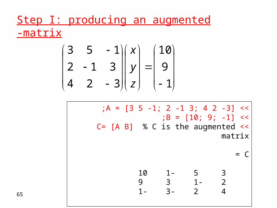
Step I: producing an augmented matrix: a matrix that consists of the Coefficient matrix, concatenated with the vector of Right hand side values.

Step II: using the function rref to produce a row-reduced echelon form of the system.

Step III: extracting the solution vector from the row-reduced echelon system

65

Step I: producing an augmented matrix-

<<A = [3 5 -1; 2 -1 3; 4 2 -3]; <<B = [10; 9; -1]; <<C= [A B] % C is the augmented matrix

C=

3 5- 1 10 2- 1 3 9 4 2- 3- 1

1

9

10

324

312

153

z

y

x

66

Step II: extracting the solution vector

>> D=rref(C) % produce a row-reduced echelon form

D =

1 0 0 1 0 1 0 2 0 0 1 3

>> x=D(:,4)‘ % extract the solution vector

x =

1 2 3

3 MATLAB code lines and we have the solution…

67

Step II: extracting the solution vector

If we had 4 equations with 3 unknowns (one equation not providing new information), we would gain nothing.Gaussian elimination would lead to same three solutions:

>> D=rref(C) % produce a row-reduced echelon form D = 1 0 0 1 0 1 0 2 0 0 1 3 0 0 0 0

68

Important point:

A system of linear equations can have no solutions, or it can have an infinite number of solutions

69

Infinitely many solutions:

Example in 2D: two equations that define the same curve

824

42

yx

yx

xy

xy

24

24

xx 2424

00

Extraction of y:

Always (for all x) true

No solutions:

Example in 2D: two equations that define parallel curves

624

42

yx

yx

xy

xy

23

24

xx 2324

34

Extraction on y:

Never true

71

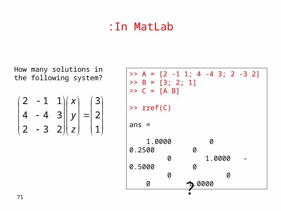
In MatLab:

>> A = [2 -1 1; 4 -4 3; 2 -3 2]>> B = [3; 2; 1]>> C = [A B]

>> rref(C)

ans =

1.0000 0 0.2500 0 0 1.0000 -0.5000 0 0 0 0 1.0000

How many solutions in the following system?

1

2

3

232

344

112

z

y

x

?

72

In MatLab:

>> A = [1 -3 1; 1 -2 3; 2 -6 2]>> B = [4; 6; 8]>> C = [A B]

>> rref(C)

ans =

1 0 7 10 0 1 2 2 0 0 0 0

How many solutions in the following system?

8

6

4

262

321

131

z

y

x

?

73

Technique 2to solve Ax = b

The inverse matrix

74

The identity matrixThe inverse matrixNon-singular and Singular matricesThe determinant

Some terminology.…

The identity matrix

An important matrix is the identity matrix, denoted by In. The identity

matrix is an nn matrix with 1s on its diagonal line and 0s elsewhere:

100

010

001

3I

Important property: if A is an m n matrix, then

AIn=ImA=A

In matrix operations, the use of the identity matrix is equivalent to the use of “1” in scalar operations.

76

The inverse matrix

Suppose that A is an n n square matrix. If there exists an n n square matrix B such that

AB = BA = In

then B is called the inverse matrix of A, and it is denoted by A-1.

Example-

22

21A

5.01

11B

10

01

5.0*221*21*2

5.0*211*21*1

5.01

11

22

21AB

10

01

2*5.022*5.01*1

2*12*12*11*1

22

21

5.01

11BA

Hence B = A-1

77

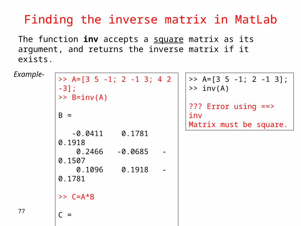
Finding the inverse matrix in MatLab

The function inv accepts a square matrix as its argument, and returns the inverse matrix if it exists.

Example->> A=[3 5 -1; 2 -1 3; 4 2 -3];>> B=inv(A)

B =

-0.0411 0.1781 0.1918 0.2466 -0.0685 -0.1507 0.1096 0.1918 -0.1781

>> C=A*B

C =

1.0000 0 0.0000 0 1.0000 0 0 0 1.0000

>> A=[3 5 -1; 2 -1 3];>> inv(A)

??? Error using ==> invMatrix must be square.

78

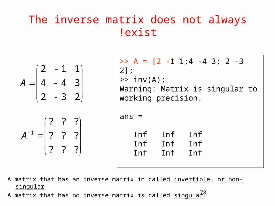
The inverse matrix does not always exist!

A matrix that has an inverse matrix in called invertible, or non-singular

A matrix that has no inverse matrix is called singular.

>> A = [2 -1 1;4 -4 3; 2 -3 2];>> inv(A);Warning: Matrix is singular to working precision.

ans =

Inf Inf Inf Inf Inf Inf Inf Inf Inf

232

344

112

A

???

???

???1A

79

Using the inverse matrix to solve a linear system

Consider the system A x = b:

if A is non-singular, we can multiply both sides, to the left, by A-1:A-1Ax = A-1b

Since A-1A=I, and since I x=x, then-

Example-x = A-1b

5

3

1

324

312

153

z

y

x

5

3

1

0.1461- 0.1573 0.0899

0.0787- 0.1461- 0.2022

0.1798 0.1910 0.0337-

5

3

1

324

312

1531

z

y

x

the inverse

80

Example-

5

3

1

324

312

153

z

y

x

5

3

1

0.1461- 0.1573 0.0899

0.0787- 0.1461- 0.2022

0.1798 0.1910 0.0337-

5

3

1

324

312

1531

z

y

x

0.1685-

0.6292-

1.4382

z

y

x

81

The determinant of a matrixAny square matrix has an associated number, which describes it (like

age isassociated with, and partially describes, a person .(

For a 2 x 2 matrix, the determinant is equal to the product of the elements on

the main diagonal minus the product of the elements on the secondary diagonal:

The determinant can be defined for any n x n matrix- However,we will not give the general formula here, since it is somewhat

complicated for n > 2 .

2221

1211

aa

aaA 21122211)det( aaaaA If Then:

The main diagonal is shown in red. The secondary diagonal is shown in blue.

82

The determinant of a matrix in MatLab

In MatLab, use the function det to find the determinant:

>> a=[2 -1 1; 4 -4 3; 2 -3 2];>> b=[3 5 1; 2 -1 3; 4 2 -3];>> fprintf(1,'%d %d',det(a),det(b))

0 89

>> A=[-1 -3; 1 -2];>> det(A)

5

83

A Matrix is invertible (non-singular) if and only if its determinant is non-zero

Take this as a fact. We will not prove this statement here.

Without explaining exactly how, the inverse matrix of matrix A can be computed by using the term 1/det(A). (see revision pages in web site for details, if you are really curious). If det(A) = 0, the term

1/det(A) is undefined, hence the inverse matrix cannot be computed.

>> b=[3 5 1; 2 -1 3; 4 2 -3];>> inv(b)

ans =

-0.0337 0.1910 0.1798 0.2022 -0.1461 -0.0787 0.0899 0.1573 -0.1461>> det(b)ans =

89

>> a=[2 -1 1; 4 -4 3; 2 -3 2];>> inv(a)Warning: Matrix is singular to working precision.

ans =

Inf Inf Inf Inf Inf Inf Inf Inf Inf>> det(a)ans =

0

84

Using the inverse matrix to solve a linear system in MatLab

<<A=[3 5 1; 2 -1 3; 4 2 -3]; <<b=[1; 3; 5];

<<x = inv(A)*b

x=

1.4382- 0.6292- 0.1685

We solved it in one line of MATLAB code…

)unless we want to test ahead of time that det(A) is not 0(

Consider the system A x = b:

85

Technique 3to solve Ax=b

Matrix Division

Matrix division:Matrix Division is equivalent to multiply by the inverse matrix. We distinguish between left division (\) and right division (/)

Left Division: A\B is equivalent to multiplying A-1 to the left of B.

A\B = A-1B

Right Division: A/B is equivalent to multiplying B-1 to the right of A.

A/B = A B-1

Hence, to solve the equation Ax = b , we left-divide both sides of the equation by A:

Ax = b A\Ax = A\b x = A\b

Matrix division to solve a linear system in MatLab

>> A=[3 5 1; 2 -1 3; 4 2 -3];>> b=[1; 3; 5];

>> x=A\b

x =

1.4382 -0.6292 -0.1685

% But not-

>> x=A/b??? Error using ==> /Matrix dimensions must agree.

>> A = [2 -1 1;4 -4 3; 2 -3 2];>> b=[1; 3; 5];>> x=A\bWarning: Matrix is singular to working precision.

x =

Inf Inf Inf

What about the cases where there is no solution?

We solved it in one line of MATLAB code, but shorter…

(unless we want to test ahead of time that det(A) is not 0 )

88

Left division is almost the same as taking the inverse of the matrix and multiplying

It is faster and more numerically stable

The Gaussian elimination method is mainly good to check your solutions…

Remember to review this lesson before next week! Lot’s of things based on it.

Graphic Objects figure axes 2D-plot 3D-plot axis labels title GUI objects pushbutton toggle edit...

Documents

Transcript of Graphic Objects figure axes 2D-plot 3D-plot axis labels title GUI objects pushbutton toggle edit...