HAL Id: hal-00825503https://hal.inria.fr/hal-00825503v2

Submitted on 12 Dec 2014

HAL is a multi-disciplinary open accessarchive for the deposit and dissemination of sci-entific research documents, whether they are pub-lished or not. The documents may come fromteaching and research institutions in France orabroad, or from public or private research centers.

L’archive ouverte pluridisciplinaire HAL, estdestinée au dépôt et à la diffusion de documentsscientifiques de niveau recherche, publiés ou non,émanant des établissements d’enseignement et derecherche français ou étrangers, des laboratoirespublics ou privés.

Graph-Theoretic Algorithms for the “Isomorphism ofPolynomials” Problem

Charles Bouillaguet, Pierre-Alain Fouque, Amandine Véber

To cite this version:Charles Bouillaguet, Pierre-Alain Fouque, Amandine Véber. Graph-Theoretic Algorithms for the“Isomorphism of Polynomials” Problem. Advances in Cryptology - 2013, May 2013, Athenes, Greece.pp.17, �10.1007/978-3-642-38348-9_13�. �hal-00825503v2�

Graph-Theoretic Algorithms for the“Isomorphism of Polynomials” Problem

Charles Bouillaguet1, Pierre-Alain Fouque2 and Amandine Veber3

1 University of Lille-1charles.bouillaguet@univ-lille1.fr

2 University of Rennes-1pierre-alain.fouque@univ-rennes1.fr

3 CMAP Lab, CNRS and Ecole Polytechniqueamandine.veber@cmap.polytechnique.fr

Abstract. We give three new algorithms to solve the “isomorphism ofpolynomial” problem, which was underlying the hardness of recoveringthe secret-key in some multivariate trapdoor one-way functions. In thisproblem, the adversary is given two quadratic functions, with the promisethat they are equal up to linear changes of coordinates. Her objective is tocompute these changes of coordinates, a task which is known to be harderthan Graph-Isomorphism. Our new algorithm build on previous work ina novel way. Exploiting the birthday paradox, we break instances of theproblem in time q2n/3 (rigorously) and qn/2 (heuristically), where qn isthe time needed to invert the quadratic trapdoor function by exhaustivesearch. These results are obtained by turning the algebraic problem intoa combinatorial one, namely that of recovering partial information onan isomorphism between two exponentially large graphs. These graphs,derived from the quadratic functions, are new tools in multivariate crypt-analysis.

1 Introduction

The notion of equivalent linear maps is a basic concept in linear algebra; twolinear functions f and g over vector spaces are equivalent if and only if there existtwo other linear bijective functions S and T such that f = T ◦g◦S. Geometricallyspeaking, this means that f and g are essentially the same function, but withcoordinates expressed in different bases. The computational problem consistingin testing the equivalence of two linear functions (given by matrices) is easy,because it is well-known that two linear maps are equivalent if and only if theyhave the same rank.

This notion of equivalent linear maps lends itself to an obvious generalization,by dropping the requirement that the functions shall be linear. Then, giventwo vector spaces U and V , of respective dimension n and m, two functionsf, g : U → V are said to be equivalent if there exist an invertible n×n matrix Sand an invertible m×m matrix T such that g = T ◦ f ◦S. Again, the geometricinterpretation of this notion is that g and f are “the same function”, up to linear

changes of coordinates. However, deciding the equivalence of two such functionsis no longer easy in general.

The case where f and g are polynomial maps is particularly relevant, notonly because it is a natural generalization of the linear case, but also because fand g admit a compact representation. It is understood that a polynomial mapf is such that each coordinate of the vector f(x) is a polynomial expression ofthe coordinates of the vector x. Testing the equivalence of two polynomial mapshas been called the “Isomorphism of Polynomials” (IP) problem by Patarin in1996 [43], and later the “Polynomial Linear Equivalence” (PLE) problem byFaugere et al. in 2006 [25].

One aspect of PLE that makes it a bit difficult to study is that dependingon the parameters (dimensions and base field of the vector spaces, degree ofthe polynomials, special restrictions, etc.), the problem can take very differentforms. We will thus focus on the case where the base field of the vector space isfinite (of size q), where polynomials are quadratic, and where their domain andcodomain are the same, i.e., where f, g : (Fq)

n → (Fq)n

are quadratic maps. Thisis the setting that appears in most cryptographic constructions. In the sequel wewill call this particular restriction the Quadratic Maps Linear Equivalence (QMLE)problem. In order to make our exposition simpler, we will furthermore assumethat q, the size of the finite field, is a power of two. The theory of quadraticforms presents itself very differently for odd characteristic and for characteristictwo, and in order not to expose two variants of each of our results, we chose themost computer-oriented setting.

The first“multivariate”cryptographic schemes relied on a somewhat heuristicconstruction to build Trapdoor One-Way Functions, whose security was basedon the hardness of QMLE. Starting with an easy-to-invert quadratic map f , onebuilds an apparently random-looking one by setting g = T ◦ f ◦ S. The ideais that the changes of coordinate would hide the structure of f that makes iteasy to invert, so that g would look random. Inverting random quadratic mapsis extremely hard, and the best options in general are exhaustive search (if q issmall), or the computation of a Groebner basis (when q is large), both techniquesbeing exponential in n. This construction backed one of the advertized goals ofmultivariate cryptography, namely the ability to encrypt or sign n-bit blockswhile offering n bits of security, as opposed to, e.g. RSA.

In this setting, g (and eventually f) is the public key, while S and T arethe secret key. When f is public, then recovering the secret-key precisely meanssolving an instance of QMLE. Several cryptosystems have been built on thisidea [10, 55, 18, 32, 15, 7], but they have all been broken [29, 24, 20, 19, 37, 29, 35,9, 28, 40, 11]. The main reason behind this fiasco is that the specific instances ofQMLE exposed by these schemes were weak because f was too special, so thatpolynomial-time and/or efficient algorithms to crack them have eventually beendesigned.

In a different direction, Patarin also proposed to use the hardness of arbi-trarily chosen instances of the PLE problem to design a public-key identificationscheme, thus potentially avoiding the aforementioned disaster. A prover, who

has generated a pair of private/public keys (PK,SK), wants to prove her iden-tity to a verifier who knows PK. In fact the prover aims to convince that sheknows SK, but without revealing any information about SK to the verifier, orto anybody else. In 1986, Goldreich, Micali and Wigderson [33] built an elegantzero-knowledge proof system for Graph Isomorphism (GI) and used it to build anidentification scheme. There, PK is a pair of isomorphic graphs, and SK is theisomorphism (a permutation of the vertices). In order for this system to be se-cure, it must be hard to solve the instance of GI formed by the public-key. Despitea large research effort, until now no algorithm has been able to solve instancesof GI in worst-case polynomial, which is certainly encouraging. However, mostinstances of GI, and in particular random instances, are extremely easy to solve.Thus, the identification scheme of [33] relied on a presumably hard problem forwhich we do not know how to generate non-trivial instances...

Patarin’s suggestion was that Graph Isomorphism could be replaced by QMLE,with the hope that random instances of the problem would then be hard, andthat key-generation would then be straightforward. There was apparently noth-ing to lose with the new problem, because it was shown to be harder than GI [44].Using random instances would in principle avoid the weak instances that hadbeen broken. The resulting QMLE-based identification scheme is not particu-larly efficient, and does not enjoy very attractive key-sizes, but it is quite simple.It also has a few interesting features compared to other identification schemesbased on NP-hard combinatorial problems such as [47–52]: most notably, it doesnot require hash functions nor commitment schemes, and it does not require theparties to share a (usually large) public common string describing an instanceof the NP-complete problem.

1.1 Related Work

The QMLE problem is reminiscent of the Even-Mansour cipher [23], which turns afixed n-bit permutation P into an n-bit block-cipher with 2n-bit key by settingEk1,k2

(x) = P (x + k1) + k2. Attacks against this construction aim to recoverthe keys while only having black-box access to E and P . One of its distinctivefeatures is that the performance of a successful adversary running in time t andsending q queries is limited by t·q ≥ 2n, under the assumption that P is a randompermutation. The known attacks match this bound [17, 22]. As mentioned above,the hardness of QMLE would allow a similar construction where a fixed andpublic quadratic permutation P is turned into a public-key encryption primitiveES,T = T ◦ P ◦ S. In this context, adversaries not only have oracle to E and P ,but know their full description.

Essentially two non-trivial algorithms have been proposed so far for QMLE:the “To-and-Fro” approach [44] on the one hand, and the “Groebner Basis” ap-proach [25] on the other hand. There are also several, more efficient algorithms forthe special case where the secret T matrix is known to be the identity matrix [31,46, 14, 36]. This sub-problem is also GI-hard, even in very restricted settings [1].The article [3] considers the particular case of testing whether two boolean func-

tions are equal modulo a permutation of their inputs. It shows that 2n/2 queriesare necessary if one only has black-box access to the boolean functions.

Back to the full QMLE problem, the “To-and-Fro” algorithm, while beingsimple, was exposed on a toy example, without pseudo-code nor detailed analyzis.We are convinced that the algorithm works when the polynomial maps f andg are bijective, but it cannot work as-is when they are not (the authors of [25]made the same observation). Note that a random polynomial map is not bijectivewith overwhelming probability. As is it given in [44], the “to-and-fro” algorithmis thus not applicable to random instances of QMLE. We found out that it isnevertheless possible to adapt the algorithm to work in the non-bijective case,but there are several ways to do so, and some are more efficient than others.Figuring that out required some work, and exposing it requires some space, sowe will not go deeper into this issue in this paper. In any case, the authorsof [44] claim that the complexity of their algorithm is of order O

(q2n)

when

q > 2 and O(23n)

when q = 2, and we agree with them. The algorithm waslater independently rediscovered under the form of a procedure to test the linearequivalence of S-boxes [12].

The “Groebner basis” algorithm, on the other hand is not heuristic, and iswell-specified. It consists in identifying coefficient-wise the equation T−1 ◦ g =f ◦ S, which relates two vectors of n quadratic forms. It is therefore equivalentto about n3 quadratic equations in the 2n2 coefficients of the unknown changesof coordinates. These equations are then solved through the computation ofa Groebner basis. The complexity of Groebner basis algorithms is notoriouslytricky to study, and the authors of [25] did not give any definitive results. How-ever, they empirically observed an important fact, namely that when f and gare inhomogeneous quadratic maps, i.e., when f and g contains non-zero linearand constant terms, then their algorithm terminated in polynomial time O

(n9).

In the homogeneous case, the authors of [25] conjectured that their algorithmis subexponential, without providing any argument nor any evidence that it isthe case. This assertion is impossible to verify in practice because the complexi-ties are too high, but our own reasoning makes us more inclined to believe thatthe algorithm is plainly exponential. Assuming that the equations form a semi-regular sequence would allow to estimate the complexity of the Groebner basiscomputation [8]; doing so results in a total complexity of O

(218n

), yet assuming

that the equations are semi-regular is probably a bit of a stretch. Establishingthe complexity of this algorithm is thus essentially an open problem.

In the sequel, we will nevertheless take for granted that inhomogeneous in-stances of QMLE are tractable and can be solved in polynomial time, using the“Groebner-based” algorithm for instance.

It must be noted that in [44], the existence of an algorithm based on thebirthday paradox and running in time O

(qn/2

)is asserted, and that this algo-

rithm is itself partially described in [45], where it is called the “combined powersattack”. This algorithm is sometimes acknowledged for in the literature (e.g.in [25]). However, it is underspecified to the point that it is impossible to imple-ment it, and some of the bits that are specified have major problems. Some of

them deterministically fail to meet their goal, and the whole construction relieson heuristic assumptions that are empirically false (sometimes provably). This“algorithm” should thus be disregarded.

1.2 Our Results

We give three algorithms to solve QMLE in the homogeneous case. All thesealgorithms work by reducing the solution of a homogeneous (hard) instance intothat of one or several inhomogeneous (easy) instances after some preprocessing.We will thus assume that we are given a (black-box) Inhomogeneous solver thatpresumably works in polynomial time, and we will count the number of inho-mogeneous queries sent to this oracle. We are well-aware that this assumptionis quite strong. The empirical success of the algorithm of [25] convinced us thatit works in polynomial-time on average, yet moving from there to “worst-casepolynomial time” seems like a leap of faith. However, this assumption eases ourexposition considerably, and in practice there does not seem to be any prob-lem (probably because the queries sent to the inhomogeneous oracle are randomenough).

Our three algorithms differ by the number of queries they send to the oracle,by the amount of computation they perform themselves, and by their successprobability.

Algo. Preprocessing Inhom. queries success prob.1 qn 12 O

(n3 · q2n/3

)q2n/3 62%

3 O(n5 · qn/2

)1 62 % only when q = 2

Algorithm 1 is deterministic, and essentially performs an exhaustive search in(Fq)

n, sending one inhomogeneous query per vector. Using the algorithm of [25]

to deal with the inhomogeneous instances, the resulting complexity isO(n9 · qn

),

which already improves on the “to-and-fro” algorithm of [44].

Algorithms 2 and 3 rely on the birthday paradox to improve on exhaustivesearch and break the qn barrier. To this end, two exponentially large isomorphicgraphs are derived from the two quadratic maps. Recovering a bit of informationon an isomorphism allows to make the problem inhomogeneous, and thus easy tosolve. The trick is that this partial information must be extracted without know-ing the full graphs, because they are too large. The construction of these graphsborrows from the differential techniques that have broken SFLASH, amongstothers.

Algorithm 2 is relatively easy to analyze and we rigorously establish its com-plexity and success probability when dealing with random instances of the prob-lem. Algorithm 3 is more efficient but more sophisticated and harder to analyze(as well as somewhat heuristic). We provide an as-rigorous-as-possible complex-ity analysis under a conjecture on random quadratic maps, and we verify exper-imentally that we are not off by too much.

Because our algorithms are exponential in n, we do not fully break Patarin’sidentification scheme (it is of no practical value anyway), even though its key-sizes should in principle be doubled. The construction of a Trapdoor One-WayFunction from QMLE outlined above has already been bludgeoned to death bycryptanalysts, and it now lies on the autopsy table. We take the role of the med-ical examiner that appears in every good police drama, only to discover that thecorpse had a fatal disease even before being brutally assaulted. We indeed believethat our algorithms condemn this generic construction of a Trapdoor One-WayFunction post-mortem, and give a theoretical reason not to try again, besides theobvious “they have all been broken” argument. Our algorithms indeed break theQMLE instance and retrieve the secret-key (asymptotically) much faster thaninverting the quadratic map by exhaustive search. This shows in passing thatthis construction can only offer n/2 bits of security, instead of the n that was itsoriginal objective.

2 A First Algorithm Based on Dehomogenization

Confronted with a homogeneous instance of QMLE, our strategy throughout thispaper is to build an inhomogeneous instance admitting the exact same solutions.This inhomogeneous instance can in turn be solved in polynomial time, andreveals the solution(s) of the original problem. The downside of this approach isthat the image of S must be known at one arbitrary point of the vector space.Indeed, if β = S · α, then:

∀x. g(x) = T · f(S · x) ⇐⇒ ∀x. g(x+ α) = T · f(S · x+ β).

Thus defining g′(x) = g(x+ α) and f ′ = f(x+ β) yields an equivalent problem,i.e., an instance that has the same solutions as the original one. In addition, thenew instance is inhomogeneous. This follows from the simple observation thatalthough x2 is a homogeneous polynomial, (x+α)2 = x2 + 2αx+α2 is not sinceit has a non-trivial linear term αx and a non-trivial constant term α2.

It follows that solving (homogeneous) instances of QMLE essentially boilsdown to finding Sα, for some known and non-zero vector α. Exhaustive searchis the first option that comes to mind, leading to Algorithm 1. This algorithmsends qn queries to the inhomogeneous solver in the worst case, and finds the so-lutions when they exist. This algorithm terminates with probability one in timeO(n9 · qn

)if the Groebner-based algorithm of [25] is used to solve the inhomoge-

neous instances. Despite being extremely simple, Algorithm 1 is asymptoticallyqn times faster than to the “to-and-fro” algorithm of [44].

This dehomogenization technique exposes a crucial asymmetry in the prob-lem: it is apparently much more critical to obtain knowledge on S than on T .This is not new: the “To-and-Fro” algorithm relies on the ability to transferknowledge of a relation β = S · α to a relation g(α) = T · f(β).

Algorithm 1 Simple algorithm based on dehomogenization.

function Exhaustive-Dehomogenization(f, g)x← random non-zero vector in (Fq)n

for all 0 6= y ∈ (Fq)n dof ′(z)← f(z + y)g′(z)← g(z + x)query IQMLE-Solver with (f ′, g′′)if solution (S, T ) found then return (S, T )

return “Not Equivalent”

3 Moving the Problem Into a Graphic World

Using the birthday paradox is a natural idea to improve on exhaustive searchalgorithms in many scenarii, with the hope to halve the exponent in the com-plexity. Here, we wish to use the birthday paradox to obtain the image of S atone point, and build a dehomogenized instance, just as we did in the previoussection. One difficulty is that we want to focus only on S, and leave T alone. Tothis end, we introduce a tool which is, to the best of our knowledge, new. Weassociate a graph Gh to any quadratic map h : (Fq)

n 7→ (Fq)n. Its vertices are

the elements of (Fq)n, and there is an edge between x, y ∈ (Fq)

nif and only if

h(x+ y) = h(x) + h(y). To some extent, Gh expresses the “linear behavior” of h(even though h is not linear) and thus we call these graphs the “linearity graphs”of the associated quadratic maps.

These graphs are natural objects associated to quadratic maps. For instance,the distinguisher of [21] to determine whether a given quadratic map f is anHFE public key can be rephrased as follows: pick a random node in Gf , andcount its neighbors. If their number exceeds a given bound (which depends onthe degree of the internal HFE polynomial), then return “random”, else return“HFE”. With the right bound on the number of neighbors, this algorithm achievessubexponential advantage.

The essential interest of linearity graphs for our purposes is that the twographs Gf and Gg are connected by the secret matrix S.

Lemma 1. If T ◦g = f ◦S then S is a graph isomorphism that sends Gf to Gg.

Proof. Indeed, if x↔ y in Gg, then by definition g(x+ y) = g(x) + g(y), and itfollows that T ◦ g(x+ y) = T ◦ g(x) + T ◦ g(y), and thus that f(S · x+ S · y) =f(S · x) + f(S · y). This in turn means that S · x ↔ S · y in Gf . It follows thatS is a graph isomorphism between Gf and Gg.

Linearity graphs thus allows a formulation of the problem where the other se-cret matrix T is no longer present. We have two (exponentially large) isomorphicgraphs Gf and Gg, and we ultimately need to recover the whole isomorphismS. However, thanks to the dehomogenization technique of the previous section,and thanks to the ease with which inhomogeneous instances can be solved, itturns out that recovering just a little bit of information on the isomorphism

is enough to find it completely. More precisely, we just need to know how theisomorphism S transforms one arbitrary vertex.

Of course, completely building these graphs is prohibitively expensive (theyhave qn vertices). It turns out that this is never necessary, because it is possibleto walk in these graphs without fully knowing them.

Walking in Linearity Graphs. The function ψ(x, y) = f(x+y)+f(x)+f(y)is a generalization of the polar form of a quadratic form to vectors thereof, incharacteristic two. It is easy to check that ψ is bilinear. Given a (non-zero) vertexx ∈ (Fq)

nin the graph, the function:

Dxf : y 7→ ψ(x, y) = f(x+ y) + f(x) + f(y)

is a familiar object in multivariate cryptology, called the Differential of f at x [27,21, 19, 29]. It is a linear function from (Fq)

nto (Fq)

n, which is then conveniently

represented by a matrix. The set of nodes adjacent to x in Gf is in fact thekernel of Dxf . Note that x always belong to ker Dxf , because x + x = 0. Themain reason we chose to focus on the case where q = 2e is that this fact is nottrue when q is not a power of two.

The matrix Dxf is easy to compute given f and x. If f is a (homogeneous)quadratic map, then it is in fact a vector of n quadratic forms, which can conve-niently be described by a collection of n matrices F1, . . . , Fn, that are interpretedas follows: Fk[i, j] is the coefficient of xixj in the k-th component of f . If tMdenotes the transpose of M , then the matrix representation of the differential off at x is given by:

Dxf =

x · (F1 + tF1) . . . x · (Fn + tFn)

.

Thus, given a vector x, finding the neighbors of x in Gf can be done intime O

(n3): computing the matrix Dxf requires n matrix-vector products, and

determining its kernel classically takes O(n3)

operations. It is thus possibleto crawl the linearity graphs by spending a polynomial number of elementaryoperations on each traversed vertex.

Structure in Linearity Graphs. Linearity graphs possess a rich structure,thanks to their algebraic origin. Recall that in Gf , two nodes x and y are adja-cent if ψ(x, y) = 0, where ψ is the symmetric bilinear map defined above. Thebilinearity of ψ induces a lot of structure in Gf . For instance, we always haveψ(x, x) = 0, and by bilinearity ψ(λx, µx) = λµψ(x, x) = 0, so that the q mul-tiples of a vector x form a clique in Gf . The set of all multiples of x are thustopologically indifferentiable (they all have the exact same neighborhood).

Furthermore, the same reasoning shows that if two vectors x and y are adja-cent in Gf , then the set of q2 linear combinations λx + µy form a clique in Gf

of size q2.

Degree Distribution. If a quadratic map f is randomly chosen (amongst thefinite number of possibilities), then the resulting linearity graph Gf follows acertain —mostly unknown— probability distribution, and any property of Gf

can be seen as a random variable. One of the most interesting properties of Gf

is the distribution of the degree (i.e., of the number of neighbors) of vertices inGf . This result is stated in terms of the probability that a random n×n matrixover Fq is invertible. We denote it by λ(n):

λ(n) =

n∏i=1

(1− 1

qi

)Lemma 2 (theorem 2 in [21]). Let x ∈ (Fq)

nbe a non-zero vector, and f :

(Fq)n → (Fq)

nbe a uniformly random quadratic map. Then Dxf is a uniformly

random matrix vanishing over x. As a consequence, the probability that Dxf hasa kernel of dimension k ≥ 1 is:

λ(n)λ(n− 1)

λ(k)λ(k − 1)λ(n− k)q−k(k−1)

Because λ(n) is a decreasing function of n that converges to a finite limitbounded away from zero, then the ratio of the λ-expressions lives in a smallinterval, independently of q, n and k, so that the probability is in fact of orderq−k(k−1). Of course, over Fq, a k-dimensional vector space contains qk elements,so that if dim ker Dxf = k, then the vertex x has qk neighbors.

Sparsity. Computing the expectation and the variance of the degree is technical,but feasible:

E [degree] = q − 1

qn−2σ2 = q2(q − 1)

(1− q2 + 1

qn+

q2

q2n

)Establishing these two expressions is somewhat technical, yet because both aresums of q-hypergeometric terms, they can be computed by “creative telescoping”thanks to the q-analog of Zeilberger’s algorithm [56]. It follows that the expectednumber of edges of Gf is essentially qn+1/2. In other terms, Gf is a very sparsegraph that has barely more edges than it has vertices.

Disconnecting Linearity Graphs. A linearity graph Gf is fully connected,because all vertices are adjacent to the “zero” vertex. This “zero” vertex is notvery interesting (since it is adjacent to every other vertex), and, as a matter offact, it even turns out to be a bit annoying. Thus, it seems that there is nothingto lose by removing it. In addition, we could also get rif of the self-loops ; theyare useless since every vertex has one.

We thus denote by G∗f the simple graph Gf in which the zero vertex hasbeen removed, and where self-edges are removed. It is interesting to note thatthe resulting graph is no longer connected, and that there are in fact very many

connected components. Indeed, if dim ker Dxf = 1, then the only neighbors of xare its multiples, and x belong to a connected component of size q−1. Lemma 2tells us that this happens with probability λ(n)/λ(1), and this converges to afinite limit bounded away from zero when n goes to infinity. Thus, a constantfraction of the vertices belong to “small” connected components of size q − 1.Working a bit on the λ functions reveals that this proportion grows like 1−1/q2.

4 Just Count Your Neighbors

It is well-know that if two graphs (V1, E1) and (V2, E2) are isomorphic, and ifρ is an isomorphism between them, then u ∈ V1 and ρ(u) ∈ V2 have the samedegree, i.e., the same number of neighbors. It follows that if u ∈ V1 and v ∈ V2do not have the same degree, then they cannot be related by ρ.

We adapt this simple idea in the context of QMLE, under the form of Al-gorithm 2. The main idea in this algorithm is to target vertices in the linearitygraphs of f and g that have a specific degree: we only look for a “right pair”y = S · x amongst vertices x, y that have a prescribed degree (chosen to opti-mise the complexity of the algorithm). The remaining of this section is devotedto establishing the properties of this algorithm, which are summarized in thefollowing theorem.

Algorithm 2 First Birthday Based Algorithm

1: function SampleSet(h)2: L← ∅3: repeat4: repeat5: x← random vertex of Gh

6: until x has q√

n/3 neighbors7: L← L ∪ {x}8: until |L| =

√2qn/3

9: return L

10: function Neighbor-Counting-QMLE(f, g)11: U ← SampleSet (f)12: V ← SampleSet (g)13: for all (x, y) ∈ U × V do14: f ′(z)← f(z + y)15: g′(z)← g(z + x)16: query IQMLE-Solver with (f ′, g′)17: if solution (S, T ) found then return (S, T )

18: return “Probably not equivalent”

Theorem 1. Algorithm 2 performs O(q2n/3

)units of computations on aver-

age, sends at most q2n/3 queries to the inhomogeneous solver, and succeeds withprobability 1− 1/e.

The helper function SampleSet returns a set of O(qn/3

)vertices of Gf

(resp. Gg), each having q√

n/3 neighbors in the graph. It follows that there areq2n/3 queries to the inhomogeneous solver, because this is the size of the cartesianproduct U × V .

It remains to establish the complexity of SampleSet, and the success prob-ability of the algorithm. As explained above, since we are looking for a “rightpair” y = S · x, it is safe to restrict our attention to vertices x, y that have aspecific degree (as long as vertices with such a degree exist in the graphs).

Lemma 2 gives us the expected number iterations of the innermost loop ofSampleSet that are required to find a random vertex with the required degree.Up to a constant factor, finding a vertex with degree qk requires qk(k−1) trials,so that finding each new random vertex requires O

(qn/3

)rank computations on

n× n matrices, hence O(n3 · qn/3

)operations.

Lemma 2 also tells us that there are on average qn−k(k−1) vertices in Gf

each having degree qk. In Algorithm 2 we look specifically at vertices of degree

q√

n/3, and we thus expect Gf to contain q2n/3 of them. Since the number ofiterations of the outermost repeat...until loop is roughly the square root of thisnumber, we do not expect more than a constant number of “extra” iterationsfinding an already-known vector x. Putting everything together, we concludethat SampleSet terminates after O

(n3q2n/3

)operations.

Now, the birthday bound tells us that U × V contains a “right pair” y = Sxwith probability greater than 63%, because both U and V contain about the

square root of the total number of vertices with degree q√

n/3 (see [53] for aprecise statement of this specific version of the birthday paradox).

Practical Results. We have implemented Algorithm 2 inside the MAGMAcomputer algebra system[13], running on one core of a 2.8 Ghz Xeon machine.As shown in Table 1, we found out that in practice it is difficult to balance thecost of building U and V on the one hand, and going through the candidate pairon the other hand, because the target degree can only take

√n integer values. We

could nevertheless verify in practice that the complexity of building the lists andthe expected number of right pairs in them is consistent with our expectations.The source code is in the public domain, and is available on the webpage ofthe first author. It uses an unpublished algorithm to solve the inhomogeneousinstances.

n q generating U and V total time logq (target degree) |U | # pairs

16 2 0s 68s 3 1 4

22 2 28s 9h45m 4 13 400

28 2 4913s 2h15m 5 8 64

Table 1. Experimental results on Algorithm 2.

5 Map Your Neighborhood

We have seen in section 3 that the linearity graphs, once deprived from the“zero”vertex, contain many small connected components. Of course, if y = Sx, thenthe connected component of x is isomorphic to the connected component of y.In this section, we describe an algorithm that builds upon this idea—instead ofjust looking at immediate neighbors, as we did in algorithm 2, we now try tolook at the whole connected component, in order to distinguish between verticesof the same degree.

Canonical Graph Labeling. Given a graph G, a Canonical Labeling algo-rithm relabels the vertices of G, thus producing a graph Canon(G), which is bydefinition isomorphic to G. The result is canonical in the sense that if G andH are isomorphic graphs, then Canon(G) = Canon(H). The canonical labelsare therefore complete invariants of the isomorphism class, and as such, com-puting a canonical labeling is necessarily harder than checking if two graphs areisomorphic. However, computing a canonical labeling can be done in averagelinear time [6], because except for an exponentially small fraction of all graphs,it can be done with a very simple linear algorithm. Deterministic algorithmsthat always succeed are subexponential, with complexity O

(exp

(√n log n

))[5].

The perhaps most well-known, and most practical algorithm dates back to 1978,and is implemented in the nauty open-source package [38]. It is known to beexponential on some specific counter-examples [39], but otherwise performs ex-ceptionally well. There are also many relevant classes of graphs where canonicallabeling is polynomial [26]: graphs of bounded degree, planar graphs, chordalgraphs, graphs of bounded treewidth, etc.

Back to our more specific problem, let us denote by Cx (resp Cy) the con-nected component of x in G∗f (resp. of y in G∗g). The key idea of the algorithmpresented in this section is that y = Sx implies Canon(Cx) = Canon(Cy). Thus,it seems that the function H : u 7→ Canon(Cu) could be used as a “hash func-tion”. In fact, in algorithm 2, we used the degree as such a “hash function”, butit was not very discriminating, because the degree does not contain enough en-tropy. We hope that H behaves as a good hash function, and that false positives,i.e., pairs (x, y) such that H(x) = H(y) but y 6= Sx, should be very rare.

One problem is that H does not distinguish between vertices of the same con-nected component. To improve it, we would need a way to single out a specificvertex in the connected component. Fortunately, most canonical labeling algo-rithm return the isomorphism (say ρ) between their argument G and Canon(G).To single a vertex x out in G, it is sufficient to send ρ(x) along with the canonicallabeling of G.

A Canonical-Labeling-Based Algorithm As discussed in section 3, G∗f con-tains many small connected components that are all isomorphic to each others,since they are all cliques of size q − 1. Therefore, if we want our “hash function”to be discriminating, we must avoid small connected components. Our “hash

function” will thus reject the vector x if there is no simple path starting from xand of length at least r. In the other direction, we cannot exclude the existenceof a giant connected component of exponential size. Therefore, we only considerthe radius-r neighborhood of the vertex x we are interested in, i.e., the set ofall vertices that can be reached from x by crossing at most r edges. This is thebasis of algorithm 3.

Algorithm 3 Canonical Labeling/Birthday Based Algorithm

1: function Hashable[r](G, x)2: Perform a Breadth-First Search in G starting from x3: return True if the BFS hits a vertex r edges away from x

4: function H[r](G, x)5: Cx ← subgraph of G formed by all vertices at most r edges away from x.6: ρ,G ← CanonicalLabeling(Cx)7: return

(G, ρ(x)

)8: function SampleHashTable(h)9: L← ∅

10: repeat11: repeat12: x← random vertex of G∗h13: until Hashable[r](G∗h, x)

14: L[H[r] (G∗h, x))

]← x

15: until |L| =√

2qn/2

16: return L

17: function Canonical-Labeling-QMLE(f, g)18: U ← SampleHashTable (f)19: V ← SampleHashTable (g)20: for all (h1 7→ x) ∈ U, (h2 7→ y) ∈ V such that h1 = h2 do21: f ′(z)← f(z + y)22: g′(z)← g(z + x)23: query IQMLE-Solver with (f ′, g′)24: if solution (S, T ) found then return (S, T )

25: return “Probably not equivalent”

Remarks on Algorithm 3. Establishing the complexity and success probabil-ity of algorithm 3 is surprisingly difficult, probably because is relies on topologicalproperties of G∗f , which is a somewhat random but very structured graph.

Algorithm 3 has been written in a generic way, independently of the actualvalue of q. However, we have only been able to discuss its properties when q = 2.We have verified that the algorithm works as we expected in this case, but thesituation when q 6= 2 is not so clear. We tend to believe that the complexity

and/or success probability degrade exponentially fast when q grows, but we fallshort of definitive conclusion.

When q = 2, the structure of G∗f seems to be richer. For instance, we alreadyalluded to the fact that the fraction of nodes whose connected component isof size only q − 1, grows like 1 − 1/q2. In addition, as we will see in the nextsection, setting q = 2 allows us to turn most more-or-less-random graphs intotrees, which are much easier to deal with.

Preliminary Analysis of Algorithm 3. When q = 2, the correctness of thealgorithm is implied by the following three heuristic statements.

Claim. i) Hashable[r](G∗f , x

)is true with probability ≈ 1/r over the random

choice of f (assuming x 6= 0).

ii) Both Hashable[r] and H[r] can be evaluated in expected time O(rn3).

iii) When restricted to elements that are Hashable[r], then H[r](G∗f , ·

)is an

εr-almost universal hash function family (indexed by f) for some ε < 1.

The notion of almost universal hash function is usually useful when the hashfunction is“less injective” than a random function. In this paper though, H[r] canbecome more injective than a random function, as soon as r becomes sufficientlylarge.

It follows from claim i that the expected number of iterations of the loop oflines 11–13 isO (r), and it follows from claim ii that finding one admissible vectorx requires O

(r2n3

)operations on average. Claim iii then guarantees that if we

choose r to be a bit larger than n, then the probability to find hash collisions canbe made smaller than 2−n, and standard birthday-type results guarantee thatthe number of expected hash collisions in the execution of SampleHashTableis constant. From this, we conclude that SampleHashTable runs in expectedtime O

(r2n3qn/2

).

It follows from the birthday paradox [53] that there is a “right pair” in U×V ,i.e., a pair (x, y) with y = Sx, with probability greater than 1 − 1/e. This isbecause (Fq)

nhas qn elements and that the sizes of both U and V are essentially

qn/2. This guarantees the success probability of the algorithm.Let us denote by N the number of bogus inhomogeneous queries, i.e., the

number of pairs x 6= y ∈ U × V with the same hash. It follows from Markov’sinequality and claim iii that P [N ≥ 1] ≤ 2qn · εr. Thus, as soon as r is asymp-totically larger than n, e.g. r = n log log n, then the probability that N ≥ 1 getsexponentially small. This concludes our preliminary analysis: algorithm 3 runsin time O

(n5qn/2

), and sends a constant number of inhomogeneous queries. It

now remains to show that our claims are valid, but we first find it reassuringto show that the practical behavior of the algorithm is very consistent with ourexpectations.

experimental results. We have implemented Algorithm 3 using the MAGMAcomputer algebra system [13], and we found out that it works well in practice,

as Table 2 shows. The experiment clearly shows that N is constant, as expected.This justify our heuristic analysis a posteriori. The implementation is in thepublic domain and is available on the webpage of the first author.

n q generating U and V finding collisions |U | N16 2 3.6 s 1s 64 6

24 2 123 s 13s 836 5

32 2 61 min 200s 11585 2

40 2 31 h 2h 165794 7

Table 2. Experimental results on Algorithm 3

6 Discussion of the Claims

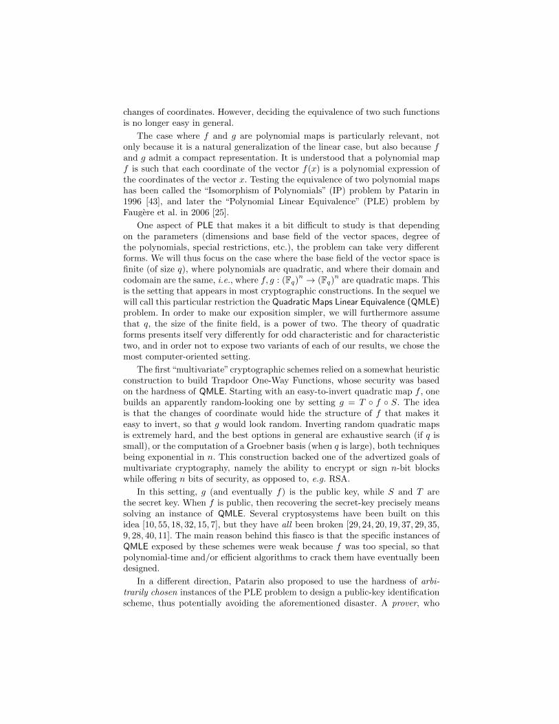
Special Structure in Linearity Graphs. Any analysis of algorithm 3 willhave to rely on the properties of linearity graphs. As argued above, the situationwhen q = 2 is somewhat different than that obtained with larger values ofq. When q = 2, the connected components of G∗f seem to enjoy a very nicestructure, as illustrated by figure 1. The origin of the triangles is that any non-isolated vertex x belong to the (q2 − 1)-clique formed by x, y and x + y (0 hasbeen removed). If it were not for these triangles, the connected components ofG∗f would be trees. While this structure is clearly visible on all the examples wecould forge, we fall short of any rigorous explanation.

x

Fig. 1. A typical moderate-size connected component of G∗f when q = 2. Self-edges arenot shown. The thick edges show a spanning tree obtained by performing a Breadth-First Search starting from x.

Conjecture 1. When r is polynomial in n, then with high probability the radius-rneighborhood of any vertex in G∗f does not contain cliques of size strictly greater

than q2− 1. In addition, every edge belongs to at most one maximal clique withhigh probability.

Back to the Trees. Fig. 1 illustrates that the connected components are closeto trees, and this analogy can easily be made rigorous when q = 2. To a vertexx in a linearity graph G∗f , we associate the unordered, unlabeled tree T [r](G∗f , x)by performing a Breadth-First Search in G∗f starting from x, and stopping redges away from x. It is well-known that any graph traversal induces a spanningtree of the graph. The tree T [r](G∗f , x) is simply the spanning tree induced bythe BFS (cf. fig. 1).

Lemma 3. If G1, G2 satisfy the properties of Conjecture 1, then:

(G1, x) isomorphic to (G2, y) ⇐⇒ ∀r. T [r](G∗1, x) isomorphic to T [r](G∗2, y)

This transformation of connected components of G∗f into trees serves severalpurposes : not only it helps understanding why our three claims hold, but is alsoallows a more efficient formulation of algorithm 3. Indeed, Hashable[r](G, x)can be evaluated by checking if T [r](G, x) has depth r. Lastly, it is well-knownthat unordered, unlabeled trees can be canonically labeled in linear time thanksto a venerable algorithm of Aho, Hopcroft and Ullman [2]. .

Random Trees From Random Linearity Graphs. When f is randomlychosen, then T [r](G∗f , x) can also be seen as a random variable. Because each

vertex of G∗f has k neighbors with some probability, then each node of T [r](G∗f , x)also has a given number of children (sometimes called “offspring” in the contextof branching processes) with some probability. Everything looks as if T [r](G∗f , x)were a random tree where the number of descendant of each node was chosen atrandom according to a given offspring distribution. The offspring distribution ofx in T [r](G∗f , x) (i.e., the root of the tree) is almost exactly the degree distributionof G∗f , which is known by lemma 2 (with the caveat that self-loops are removed).However, the offspring distribution of non-root nodes is a bit different:

`n(i) = P [a non-root node produces i offspring] =

{pn,k when i = qk − q2

0 otherwise

where

pn,k = P[dim kerDxf = k

∣∣y ∈ kerDxf]

=λ(n)λ(n− 2)

λ(k)λ(k − 2)λ(n− k)· q−k(k−2)

The expression of pn,k can be derived from a reasoning similar to that of theproof of lemma 2, which can also be found in [21]. It is also possible to compute

the expected progeny µ of each non-root node, and the variance σ2 of the offspringdistribution :

µ = 1− 1

qn−2σ2 = q2(q − 1)

(1− q2 + 1

qn+

q2

q2n

)These two expressions can be derived from the expectation and the variance ofthe degree in Gf without too much effort.

When a random tree is sampled by choosing independently the number ofchildren of each node according to a fixed law, the resulting object is called arandom Galton-Watson tree. These random trees are well-studied [4], and thiswealth of results would be extremely useful to our own purposes. Unfortunately,in T [r](G∗f , x), the number of descendant of each node is not even pairwise-independent.

We nevertheless denote by Pn the law of Galton-Watson trees with offspring

distribution `n, and by P[r]n the law of such trees conditioned to be of height at

least r. We verified in practice that the following assumption holds very well.

Heuristic Assumption: Over the random choice of f , T [r](G∗f , x) has the same

properties as Galton-Watson trees sampled according to P[r]n and truncated at

depth r.

Because µ ≤ 1, trees sampled according to Pn are finite with probabilityone [4]. In addition, the probability that a tree sampled according to Pn hasheight greater than r is equivalent to 2/(rσ2) ≈ 2/(r · q3) [4]. This justifiesclaim i.

However, it follows from this result that the expected height of trees sampledaccording to Pn is not finite; this justifies why we stop the BFS after a (finite)depth. It is also known that in trees sampled according to Pn, the expectedtotal number of nodes after h generation is h + 1 [42]. It follows that actuallyperforming the BFS requires on average O (r) matrix operations. This justifiesclaim ii.

False Positive Rate. It remains to justify claim iii, the trickiest one. Underthe heuristic assumption that T [r](G∗f , x) follows the law Pn, then claim iiiis equivalent to the following statement: the probability that two random trees

sampled according to P[r]n are isomorphic decreases exponentially fast with r.

In other word, we must determine the probability that two random trees areisomorphic. While this appears to be a natural question, it has (to the best ofour knowledge) not been treated in the literature. We could not establish therequired exponential upper-bound in general, however we proved a strong enoughbound that holds if we are allowed to reject a negligible amount of trees (i.e.,

shrinking a bit the Hashable[r] domain).We say that a tree has a unique spine decomposition if there is a unique path

starting from the root and reaching a leaf of maximal depth. We also say thata tree has a unique spine decomposition up to height k if there is a unique pathstarting from the root and reaching depth k that extends to a path reaching

nodes of maximal depth. Fig 2 shows a tree with a spine decomposition up toa certain level. Note that it is easy (and efficient) to check whether a given treehas this property. We now redefine the hashable domain by saying that x ∈ G isHashable[h,r] if and only if T [h](G, x) has depth at least h, and admits a uniquespine decomposition up to height r.

h

r

Fig. 2. A Tree of height h with a spine decomposition up height r.

Theorem 2. There exists constants c, d such that the probability that a random

tree sampled according to P[h]n has a spine decomposition up to height r is greater

than 1− c · (r/h)− c/r.

Informally speaking, this theorem means than enforcing the existence of aunique spine decomposition up to some height does not really shrink the hash-able domain. For instance, one may pick h = n log n and r = n log log n. Withthese values, trees of height h have a unique spine decomposition up to height rasymptotically almost surely.

Theorem 3. There is a constant ε ∈]0; 1[ such that if two trees sampled accord-

ing to P[h]n have a unique spine decomposition up to height r, then the probability

that they are isomorphic is upper-bounded by εr.

This justifies claim iii. Proofs of these two theorems can be found in Ap-pendix B. We conclude that modifying the definition of Hashable(G, x) to onlyaccept x if T [h](G, x) has height h and a unique spine decomposition under height

r, with h = n log n and r = n log log n is enough to make algorithm 3 work asadvertised.

References

1. Agrawal, M., Saxena, N.: Equivalence of f-algebras and cubic forms. In Durand, B.,Thomas, W., eds.: STACS. Volume 3884 of Lecture Notes in Computer Science.,Springer (2006) 115–126

2. Aho, A.V., Hopcroft, J.E., Ullman, J.D.: The Design and Analysis of ComputerAlgorithms. Addison-Wesley Publishing Company (1974)

3. Alon, N., Blais, E.: Testing boolean function isomorphism. In Serna, M.J., Shaltiel,R., Jansen, K., Rolim, J.D.P., eds.: APPROX-RANDOM. Volume 6302 of LectureNotes in Computer Science., Springer (2010) 394–405

4. Athreya, K.B., Ney, P.: Branching processes. Springer-Verlag, Berlin, New York,(1972)

5. Babai, L., Kantor, W.M., Luks, E.M.: Computational complexity and the classifi-cation of finite simple groups. In: FOCS, IEEE Computer Society (1983) 162–171

6. Babai, L., Kucera, L.: Canonical labelling of graphs in linear average time. In:FOCS, IEEE Computer Society (1979) 39–46

7. Baena, J., Clough, C., Ding, J.: Square-vinegar signature scheme. In: PQCrypto’08: Proceedings of the 2nd International Workshop on Post-Quantum Cryptogra-phy, Berlin, Heidelberg, Springer-Verlag (2008) 17–30

8. Bardet, M., Faugere, J.C., Salvy, B.: On the complexity of Grobner basis compu-tation of semi-regular overdetermined algebraic equations. In: Proc. InternationalConference on Polynomial System Solving (ICPSS). (2004) 71–75

9. Bettale, L., Faugere, J.C., Perret, L.: Cryptanalysis of the trms signature schemeof pkc’05. In Vaudenay, S., ed.: AFRICACRYPT. Volume 5023 of Lecture Notesin Computer Science., Springer (2008) 143–155

10. Billet, O., Gilbert, H.: A traceable block cipher. In Laih, C.S., ed.: ASIACRYPT.Volume 2894 of Lecture Notes in Computer Science., Springer (2003) 331–346

11. Billet, O., Macario-Rat, G.: Cryptanalysis of the square cryptosystems. In Mat-sui, M., ed.: ASIACRYPT. Volume 5912 of Lecture Notes in Computer Science.,Springer (2009) 451–468

12. Biryukov, A., Canniere, C.D., Braeken, A., Preneel, B.: A toolbox for cryptanalysis:Linear and affine equivalence algorithms. In: EUROCRYPT. (2003) 33–50

13. Bosma, W., Cannon, J.J., Playoust, C.: The Magma Algebra System I: The UserLanguage. J. Symb. Comput. 24(3/4) (1997) 235–265

14. Bouillaguet, C., Faugere, J.C., Fouque, P.A., Perret, L.: Practical cryptanalysisof the identification scheme based on the isomorphism of polynomial with onesecret problem. In Catalano, D., Fazio, N., Gennaro, R., Nicolosi, A., eds.: PublicKey Cryptography. Volume 6571 of Lecture Notes in Computer Science., Springer(2011) 473–493

15. Clough, C., Baena, J., Ding, J., Yang, B.Y., Chen, M.S.: Square, a new multivariateencryption scheme. In Fischlin, M., ed.: CT-RSA. Volume 5473 of Lecture Notesin Computer Science., Springer (2009) 252–264

16. Cramer, R., ed.: Advances in Cryptology - EUROCRYPT 2005, 24th Annual Inter-national Conference on the Theory and Applications of Cryptographic Techniques,Aarhus, Denmark, May 22-26, 2005, Proceedings. In Cramer, R., ed.: EURO-CRYPT’05. Volume 3494 of Lecture Notes in Computer Science., Springer (2005)

17. Daemen, J.: Limitations of the even-mansour construction. [34] 495–49818. Ding, J., Wolf, C., Yang, B.Y.: -invertible cycles for multivariate quadratic public

key cryptography`. In Okamoto, T., Wang, X., eds.: Public Key Cryptography.Volume 4450 of Lecture Notes in Computer Science., Springer (2007) 266–281

19. Dubois, V., Fouque, P.A., Shamir, A., Stern, J.: Practical Cryptanalysis ofSFLASH. In: CRYPTO. Volume 4622., Springer (2007) 1–12

20. Dubois, V., Fouque, P.A., Stern, J.: Cryptanalysis of SFLASH with Slightly Mod-ified Parameters. In: EUROCRYPT. Volume 4515., Springer (2007) 264–275

21. Dubois, V., Granboulan, L., Stern, J.: An efficient provable distinguisher for hfe.In Bugliesi, M., Preneel, B., Sassone, V., Wegener, I., eds.: ICALP (2). Volume4052 of Lecture Notes in Computer Science., Springer (2006) 156–167

22. Dunkelman, O., Keller, N., Shamir, A.: Minimalism in cryptography: The even-mansour scheme revisited. In Pointcheval, D., Johansson, T., eds.: EUROCRYPT.Volume 7237 of Lecture Notes in Computer Science., Springer (2012) 336–354

23. Even, S., Mansour, Y.: A construction of a cioher from a single pseudorandompermutation. [34] 210–224

24. Faugere, J.C., Joux, A., Perret, L., Treger, J.: Cryptanalysis of the hidden matrixcryptosystem. In Abdalla, M., Barreto, P.S.L.M., eds.: LATINCRYPT. Volume6212 of Lecture Notes in Computer Science., Springer (2010) 241–254

25. Faugere, J.C., Perret, L.: Polynomial Equivalence Problems: Algorithmic and The-oretical Aspects. In Vaudenay, S., ed.: EUROCRYPT. Volume 4004 of LectureNotes in Computer Science., Springer (2006) 30–47

26. Fortin, S.: The graph isomorphism problem. Technical report, University of Alberta(1996)

27. Fouque, P.A., Granboulan, L., Stern, J.: Differential cryptanalysis for multivariateschemes. [16] 341–353

28. Fouque, P.A., Macario-Rat, G., Perret, L., Stern, J.: Total break of the `-ic sig-nature scheme. In Cramer, R., ed.: Public Key Cryptography. Volume 4939 ofLecture Notes in Computer Science., Springer (2008) 1–17

29. Fouque, P.A., Macario-Rat, G., Stern, J.: Key Recovery on Hidden MonomialMultivariate Schemes. In Smart, N.P., ed.: EUROCRYPT. Volume 4965 of LectureNotes in Computer Science., Springer (2008) 19–30

30. Geiger, J.: Elementary new proofs of classical limit theorems for Galton-Watsonprocesses. J. Appl. Probab. 36(2) (1999) 301–309

31. Geiselmann, W., Meier, W., Steinwandt, R.: An Attack on the Isomorphisms ofPolynomials Problem with One Secret. Int. J. Inf. Sec. 2(1) (2003) 59–64

32. Gligoroski, D., Markovski, S., Knapskog, S.J.: Multivariate quadratic trapdoorfunctions based on multivariate quadratic quasigroups. In: Proceedings of theAmerican Conference on Applied Mathematics, Stevens Point, Wisconsin, USA,World Scientific and Engineering Academy and Society (WSEAS) (2008) 44–49

33. Goldreich, O., Micali, S., Wigderson, A.: Proofs that yield nothing but their valid-ity and a methodology of cryptographic protocol design (extended abstract). In:FOCS, IEEE (1986) 174–187

34. Imai, H., Rivest, R.L., Matsumoto, T., eds.: Advances in Cryptology - ASI-ACRYPT ’91, International Conference on the Theory and Applications of Cryp-tology, Fujiyoshida, Japan, November 11-14, 1991, Proceedings. In Imai, H., Rivest,R.L., Matsumoto, T., eds.: ASIACRYPT. Volume 739 of Lecture Notes in Com-puter Science., Springer (1993)

35. Joux, A., Kunz-Jacques, S., Muller, F., Ricordel, P.M.: Cryptanalysis of thetractable rational map cryptosystem. [54] 258–274

36. Kayal, N.: Efficient algorithms for some special cases of the polynomial equivalenceproblem. In Randall, D., ed.: SODA, SIAM (2011) 1409–1421

37. Macario-Rat, G.: Cryptanalyse de schemas multivaries et resolution du problemeIsomorphisme de Polynomes. PhD thesis, Universite Paris Diderot — Paris 7 (June2010)

38. McKay, B.: Computing automorphisms and canonical labelling of graphs. In:Lecture Notes in Mathematics. (1978) 223–232

39. Miyazaki, T.: The complexity of mckay’s canonical labelling algorithm. In Finkel-stein, L., Kantor, W.M., eds.: Groups and computation, II. Volume 28 of DIMACS:Series in Discrete Mathematics and Theoretical Computer Science., AMS and DI-MACS (1997) 239–256

40. Mohamed, M., Ding, J., Buchmann, J., Werner, F.: Algebraic attack on the mqqpublic key cryptosystem. In Garay, J., Miyaji, A., Otsuka, A., eds.: Cryptology andNetwork Security. Volume 5888 of Lecture Notes in Computer Science. SpringerBerlin / Heidelberg (2009) 392–401

41. Monagan, M.B., Geddes, K.O., Heal, K.M., Labahn, G., Vorkoetter, S.M., McCar-ron, J., DeMarco, P.: Maple 10 Programming Guide. Maplesoft, Waterloo ON,Canada (2005)

42. Pakes, A.G.: Some limit theorems for the total progeny of a branching process.Advances in Applied Probability 3(1) (1971) 176–192

43. Patarin, J.: Hidden fields equations (hfe) and isomorphisms of polynomials (ip):Two new families of asymmetric algorithms. In: EUROCRYPT. (1996) 33–48

44. Patarin, J., Goubin, L., Courtois, N.: Improved Algorithms for Isomorphisms ofPolynomials. In: EUROCRYPT. (1998) 184–200

45. Patarin, J., Goubin, L., Courtois, N.: Improved Algorithms for Isomorphisms ofPolynomials – Extended Version. available at http://minrank.org/ip6long.pdf

(1998)46. Perret, L.: A Fast Cryptanalysis of the Isomorphism of Polynomials with One

Secret Problem. [16] 354–37047. Pointcheval, D.: A new identification scheme based on the perceptrons problem.

In: EUROCRYPT. (1995) 319–32848. Sakumoto, K.: Public-key identification schemes based on multivariate cubic poly-

nomials. In Fischlin, M., Buchmann, J., Manulis, M., eds.: Public Key Cryptogra-phy. Volume 7293 of Lecture Notes in Computer Science., Springer (2012) 172–189

49. Sakumoto, K., Shirai, T., Hiwatari, H.: Public-key identification schemes based onmultivariate quadratic polynomials. In Rogaway, P., ed.: CRYPTO. Volume 6841of Lecture Notes in Computer Science., Springer (2011) 706–723

50. Shamir, A.: An efficient identification scheme based on permuted kernels (ex-tended abstract). In Brassard, G., ed.: CRYPTO. Volume 435 of Lecture Notes inComputer Science., Springer (1989) 606–609

51. Stern, J.: A new identification scheme based on syndrome decoding. In Stinson,D.R., ed.: CRYPTO. Volume 773 of Lecture Notes in Computer Science., Springer(1993) 13–21

52. Stern, J.: Designing identification schemes with keys of short size. In Desmedt,Y., ed.: CRYPTO. Volume 839 of Lecture Notes in Computer Science., Springer(1994) 164–173

53. Vaudenay, S.: A Classical Introduction to Cryptography: Applications for Com-munications Security. Springer-Verlag New York, Inc., Secaucus, NJ, USA (2005)

54. Vaudenay, S., ed.: Public Key Cryptography - PKC 2005, 8th International Work-shop on Theory and Practice in Public Key Cryptography, Les Diablerets, Switzer-

land, January 23-26, 2005, Proceedings. In Vaudenay, S., ed.: Public Key Cryp-tography. Volume 3386 of Lecture Notes in Computer Science., Springer (2005)

55. Wang, L.C., Hu, Y.H., Lai, F., yen Chou, C., Yang, B.Y.: Tractable rational mapsignature. [54] 244–257

56. Wilf, H., Zeilberger, D.: An algorithmic proof theory for hypergeometric (ordinaryand ”q”) multisum/integral identities. Inventiones Mathematicae 108 (1992) 575–633 10.1007/BF02100618.

A Expected Progeny and Variance

By definition the expected progeny is:

µ =

n∑k=2

pn,k(qk − q2

)Via an analog of lemma 2, this can be rephrased in terms of the properties of arandom linear map h. Indeed, it is shown in [21] that:

pn,k = P[dim kerDxf = k

∣∣y ∈ kerDxf]

= P[dim kerh = k

∣∣x, y ∈ kerh]

And therefore:

µ =

(n∑

k=2

P[dim kerh = k

∣∣x, y ∈ kerh]qk

)− q2

The sum is in fact the expected cardinality of the kernel of a random linear mapknown to vanish on a fixed 2-dimensional subspace:

µ = E[card kerh

∣∣x, y ∈ ker f]− q2

Thus, to establish the expression of µ, we determine the expected cardinality ofthe kernel of a random linear map h known to vanish on a fixed subspace F ofdimension s. Even though this seems to be an elementary question, we could notfind the result in the existing literature.

Lemma 4. Let h be a uniformly random endomorphism of (Fq)n

, vanishing ona subspace F of (Fq)

n, with dimF = s. Then:

E[card kerh

∣∣F ⊆ ker f]

= qs + 1− 1

qn−s

This lemma establishes the expression of µ (and we postpone its proof a littlebit). Let us now turn our attention to the variance σ2:

σ2 =

[n∑

k=2

pn,k(qk − q2

)2]− µ2

=

(n∑

k=2

pn,k · q2k)− 2q2

(n∑

k=2

pn,k · qk)

+ q4 − µ2

=

(n∑

k=2

pn,k · q2k)−

(n∑

k=2

pn,k · qk)2

Thanks to the relation between pn,k and random linear maps outlined above, wesee that σ2 is in fact exactly the variance of the cardinality of the kernel of arandom linear map known to vanish on two fixed vectors.

Lemma 5. Let h be a uniformly random endomorphism of (Fq)n

, vanishing ona subspace F of (Fq)

n, with dimF = s. Then the variance of the cardinality of

its kernel is:

qs(q − 1)

(1− qs + 1

qn+

qs

q2n

)This establishes the expression of σ2. We know give the proofs of the two lemma.

Proof (of lemma 4).

En = E[card ker f

∣∣F ⊆ ker f]

=

n∑k=s

P[dim ker f = k

∣∣F ⊆ ker f]qk

=

n∑k=s

λ(n)λ(n− s)λ(k)λ(k − s)λ(n− k)

q−k(k−s)qk

A combinatorial and/or elementary argument completely eluded us. We there-fore use the method of “creative telescoping” to establish the result by inductionon n. First, we notice that the announced results holds when n = s. Let ustherefore assume n > s. We denote by T (n, k, s) the hairy term under the sum.It is a q-hypergeometric term because if we set X = qn and Y = qk, we see thatthe two following ratios are rational functions of X and Y :

T (n+ 1, k, s)

T (n, k, s)=q2X2 − (q + qs+1)X + qs

q2X2 − qXYT (n, k + 1, s)

T (n, k, s)= qs+2 X + Y

X (qY − qs) (qY − 1)

We thus used the q-analog of Zeilberger’s algorithm [56] (as implemented inMaple [41]), and it found the nice recurrence relation:

a · T (n+ 1, k, s)− b · T (n, k, s) = g(n, k + 1, s)− g(n, k, s) (?)

where:

a = qn+1 + qn+s+1 − qs+1

b = qn+1 + qn+1+s − qs

g(n, k, s) =

(qk − qs

) (qk − 1

) (qn+s+1 − qn+s+2 − qk+s + qn+k+1 + qn+k+s+1

)q2k (qn+1 − qk)

T (n, k, s)

The point is that summing (?) over k = s, . . . , n− 1 yields:

a (En+1 − T (n+ 1, n+ 1, s)− T (n+ 1, n, s))−b (En − T (n, n, s)) = g(n, n, s)−g(n, s, s)

At this point, it is easy to find that g(n, s, s) = 0, and we check (using a computeralgebra system!) that:

g(n, n, s) + a · (T (n+ 1, n+ 1, s) + T (n+ 1, n, s)) + b · T (n, n, s) = 0

Thus, we have established that:(1 + qs − 1

qn−s

)En+1 =

(1 + qs − 1

qn+1−s

)En

Thus, if the result holds at rank n, then it also holds at rank n+ 1. ut

Proof (of lemma 5). The variance is:

Vn =

n∑k=s

(λ(n)λ(n− s)

λ(k)λ(k − s)λ(n− k)q−k(k−s)

)q2k︸ ︷︷ ︸

Un

−(qs + 1− 1

qn−s

)2

We will first demonstrate by induction on n ≥ s that:

Un = q2s + 1 + (1 + q)

(qs − 1

qn−s− 1

qn−2s

)+

1

q2n−1−2s(♣)

When n = s, we should have Un = q2n, and looking at (♣) carefully revealsthat our expression of Un simplifies to this value. Let us therefore assume n > s,and let us again denote by T (n, k, s) the hairy term under the sum. It is againa q-hypergeometric term, and running the q-analog of Zeilberger’s algorithmyields:

a · T (n+ 1, k, s)− b · T (n, k, s) = g(n, k, s)− g(n, k + 1, s) (?)

where:

a = −qn+s+2 + qs+1+2n + q1+2n + q2s+2 − q2s+n+1 − qs+1+n − q2s+2+n + q2s+2n+1 + qs+2+2n

b = −q1+2n + qn+s − qs+1+2n + qs+1+n − q2s + q2s+n+1 + q2s+n − q2s+2n+1 − qs+2+2n

g is a complicated term with a singularity when n+ 1 = k. We again notice thatg(n, s, s) = 0 and that:

a · T (n+ 1, n+ 1, s) + a · T (n+ 1, n, s)− b · T (n, n, s) = g(n, n, s)

So that summing (?) over k = s, . . . , n− 1 and exploiting the previous equationyields:

a · Un+1 = b · Un

By induction hypothesis, (♣) holds at rank n. Plugging the expression of Un intothis recurrence relation and simplifying shows that (♣) holds at rank n + 1 —please use a computer algebra system if you really want to verify this. Movingback to the expression of Vn, it is not difficult to verify that the result of thelemma holds. ut

B Isomorphism of Random Trees

For any n ≥ 3, let T be a tree sampled according to P (i.e., with offspringdistribution `), and let P[h] be the law of T conditioned to have height at leasth.

In this section, all quantities depend on n (the random tree T, the law P[h],the offspring distribution `, the height h, etc.), but we do not always make thisdependency explicitly visible by writing subscripts or superscripts, in order tomake notations less cumbersome. In addition, we also write P[h][·] instead ofP[·∣∣Height(T) ≥ h

].

We need a criterion to decide whether two conditioned trees are isomorphic ornot, and we need it to be simple enough so that we may evaluate the probabilitythat it holds. The criterion we will use is the following: two isomorphic treeswith a unique spine decomposition must have empty subtrees emanating fromthe backbone at the exact same heights. Of course, if the spine decomposition isunique up to height r, then this holds only up to height r. This will intuitivelyshow that two random trees with a unique spine decomposition up to height rare isomorphic with a probability that gets exponentially small in r. We willmake this intuition formal later, but we must first introduce some properties ofthe spine decomposition.

We decompose a conditioned tree (i.e., a tree of law P[h]) into a backbone(or spine) going from the root to height h, on which we graft a given number ofunconditioned Galton-Watson trees at each of its nodes. Looking at all nodes ofheight r, if only one of them has descendants at height h then the spine up toheight r is uniquely determined: necessarily, it is the path in the tree going fromthe root to this node (fig. 2 illustrates this).

Let us work for a moment with ordered Galton-Watson trees. That is, we alsorecord who is the descendant of each parent and offspring are ordered (so thatwe can talk about brothers to the left or to the right of an individual). In [30],Geiger shows that if we define the sequence of independent random variables(Vm, Ym) ,m ∈ N by

P [Vm = j, Ym = k] =P [Height(T) ≥ m− 1]

P [Height(T) ≥ m]·P [Height(T) < m− 1]

j−1 · `(k),

for 1 ≤ j ≤ k <∞, then Tn conditioned to have height at least h has the samelaw as the random tree constructed inductively as follows:

– The root (i.e., the first node of the spine) has Yh offspring.– To each of the Vh−1 first offspring node we graft a Galton-Watson tree with

offspring distribution ` and conditioned to have height (strictly) less thanh − 1. These Vh − 1 trees are independent of each other (and of the rest ofthe construction). These subtrees are on the left of the backbone on fig. 3.

– To each of the Yh − Vh last offspring, we graft an unconditioned Galton-Watson tree with offspring distribution ` (again, these trees are independentof each other and of the rest of the construction). These subtrees are on theright of the backbone on fig. 3.

Fig. 3. Illustration of the spine decomposition (this is Figure 1 from [30]). This showsthe Galton-Watson tree conditionned on non-extinction at generation n and n + 1respectively. GW (k) denotes a Galton-Watson tree conditioned to be extinct at gen-eration k. The subtrees to the right of the line of descent of the left-most particle areordinary Galton-Watson trees.

– The Vh-th offspring node continues the spine. It has Yh−1 offspring, thefirst Vh−1 ones are the roots of i.i.d. Galton-Watson trees conditioned tohave height less than h − 2, the last Yh−1 − Vh−1 are the roots of i.i.d.unconditioned Galton-Watson trees and the spine carries on with the Vh−1-th offspring, which has Yh−2 offspring nodes, and so on.

Observe that the marginal distribution of Ym is given by

P [Ym = y] =1− P [Height(T) < m− 1]

y

P [Height(T) ≥ m]· `(y), (1)

The spine can be seen as a“prolific” line of descent that survives up to generationh by producing a biased number of offspring, while the other individuals of thepopulation reproduce essentially according to the initial offspring distribution(we refer to [30] for an explanation of the fact that trees emanating from brothersto the left of the spine are conditioned not to have descendants at generation h).

Proof (proof of theorem 2). We show that in a tree sampled according to P[h],with high probability only one path from the root to height r extends to a pathreaching height h. Call this event A. Since this property is purely topological,then it does not matter whether the tree is ordered or not. We obtain the desiredresult by bounding from below the probability of A by the probability that alltrees emanating from the spine under height r are of height less than h− r. Theindependence of this family of trees, together with the fact (easy to check) thatfor every integer i in the interval {1, . . . , r − 1}

P[Height(T) < h− r

∣∣Height(T) < h− i]≥ P [Height(T) < h− r] ,

enables us to write

P [A] ≥r−1∏i=0

E[P [Height(T) < h− r]Yh−i−1

]≥ E

[P [Height(T) < h− r]

∑r−1i=0 Yh−i

]. (2)

Now, as n→ +∞, all the pn,k (for k ∈ {3, . . . , n}) converge to a finite limit p∞,k

, the expected progeny µ converges to 1 (recall that µ < 1 for every n), andfinally the variance σ2

n converges to q3 − q2. The last two convergences happenexponentially fast in n, therefore the same proof as that of Theorem 3.1 in [30](in which µ = 1 for all n) shows that whenever (mn)n≥1 tends to infinity at mostpolynomially, we have

limn→∞

mn · P [Height(T) ≥ mn] =2

σ2. (3)

Furthermore, we have the following lemma.

Lemma 6. There exist constants C3, C4 > 0 such that for every n ≥ 3,

P

[r−1∑i=0

Yh−i > rC3

]≤ C4

r.

We postpone the proof of Lemma 6 until the end of the proof of Theorem 2.Armed with (3) and Lemma 6, we can come back to (2) and write for every n

P [A] ≥ E[P [Height(T) < h− r]rC3 · 1{∑r−1

i=0 Yh−i≤C3r}]

≥(

1− C4

σ2h

)rC3

× P

[r−1∑i=0

Yh−i ≤ rC3

]

≥ e− rhC6

(1− C4

r

)≥ 1− r

hC7. (4)

Note that for the third inequality, use the fact that 1 − x ≥ e−2x for everyx ∈ [0, 1/2]. What (4) shows is that for every n ≥ 3, if we sample a Galton-Watson tree T according to P[h], then with probability at least 1 − C7

rh there

will be a unique spine decomposition under height r.

Proof (of lemma 6). We use Markov’s inequality (in a Chebychev-like fashion)as follows: if C3 > 0, we have for each n ≥ 3

P

[r−1∑i=0

Yh−i > rC3

]= P

[r−1∑i=0

(Yh−i − E [Yh−i]) > C3 · r −r−1∑i=0

E [Yh−i]

]

≤

E

(r−1∑i=0

(Yh−i − E [Yh−i])

)2

(C3 · r −

r−1∑i=0

E [Yh−i]

)2 . (5)

Let us show that the numerator in the right-hand side of (5) is of order r, whilethe denominator is of order r2 whenever C3 > 0 is large enough. These two pointsrely on appropriate bounds on the first two moments of all Yh−i’s (observe thatthe numerator is in fact the sum of the variances of the Yh−i’s). Indeed, recallfrom (1) that for every k ∈ {3, . . . , n},

P[Yh−i = qk − q2

]=

1− P [Height(T) < h− i− 1]qk−q2

P [Height(T) ≥ h− i]· pn,k

and these are the only possible values for Yh−i. Because 1−e−x ≤ x for all x ≥ 0,we can write for every i ≤ r − 1 :

1− P [Height(T) < h− i− 1]qk−q2 ≤ −

(qk − q2

)logP [Height(T) < h− i− 1]

≤ −(qk − q2

)logP [Height(T) < h− r − 2] .

We thus have for every such integer i

1− P [Height(T) < h− i− 1]qk−q2

(qk − q2) · P [Height(T) ≥ h− i]≤ − logP [Height(T) < h− r − 2]

P [Height(T) ≥ h].

Moreover, because λ(·) is decreasing,

λ(n)λ(n− 2)

λ(k)λ(k − 2)λ(n− k)≤ lim

n→∞

1

λ(n)=: Cq.

Combining the above, we arrive at

P[Yh−i = qk − q2

]≤ − logP [Height(T) < h− r − 2]

P [Height(T) ≥ h]· Cq ·

(qk − q2

)q−k(k−2)

for every n ≥ 3 and k ∈ {2, . . . , n}. This yields

E [Yh−i] ≤ −logP [Height(T) < h− r − 2]

P [Height(T) ≥ h]· Cq ·

n∑k=3

(qk − q2

)2q−k(k−2)

E[(Yh−i)

2]≤ − logP [Height(T) < h− r − 2]

P [Height(T) ≥ h]· Cq ·

n∑k=2

(qk − q2

)3q−k(k−2)

Now, by (3) we have

limn→∞

− logP [Height(T) < h− r − 2]

P [Height(T) ≥ h]= 1,

and furthermore,

∞∑k=3

(qk − q2

)2q−k(k−2) =: m1 <∞ and

∞∑k=3

(qk − q2

)3q−k(k−2) =: m2 <∞.

As a consequence, there exists C > 0 such that for every n ≥ 3, we have

r−1∑i=0

E [Yh−i] ≤ Cm1r,

and (using the independence of all Ym’s)

E

(r−1∑i=0

Yh−i − E [Yh−i]

)2 =

r−1∑i=0

Var (Yh−i) ≤ rC ′,

for a constant C ′ > 0 depending on m1 and m2. Choosing C3 > Cm1 and comingback to (5), we obtain the existence of C4 > 0 such that for every n ≥ 3,

P

[r−1∑i=0

Yh−i ≥ rC3

]≤ C4

r.

This completes the proof of Lemma 6. ut

Proof (proof of theorem 3). Let us use again T (from the proof of theorem 2)and its spine decomposition under the additional conditioning that all treesemanating from the spine under height r are of height smaller than h − r. Wewrite P[h][·] as a shorthand for this conditionnal probability. By construction,each brother of the i-th node of the spine (0 ≤ i ≤ r − 1) has no offspring withprobability

e := P[T = ∅

∣∣Height(T) ≤ h− r]

=P [T = ∅]

P [Height(T) ≤ h− r]=

`n(0)

P [Height(T) ≤ h− r].

(6)

Brother to the right or to the left does not matter here since the condition at thedenominator is stronger than Height(T) < h − i − 1 for our range of integersi. Let us use (6) to obtain some bounds (away from 0 and 1), uniform in n andi ≤ r− 1, for the probability that all of the Yh−i− 1 brothers of the i-th node ofthe spine have zero offspring. Because `(0) = pn,2 and using (3), the right-handside of (6) is equivalent as n→∞ to

`(0)

1− 2/(σ2 · h)'

n→∞lim

n→∞

λ(n)

λ(2)=: e ∈]0, 1[. (7)

Thus, if we denote α = P[h] [no nephews at height i], then by definition

α ≥ P[Yh−i = q3 − q2

]· (e)q

3−q2−1

Using (1) and (3),

α ≥1−

(1− 2

σ2(h− i− 1)+ o

(1h

))q3−q2

2

σ2(h− i)+ o

(1h

) · pn,2 · (e)q3−q2−1

The fraction is equal to q3 − q2 + o(1/(h)), and given the expression of pn,3 aswell as (7), the lower bound on α is equivalent to

q3 − q2

q3· e

q3−q2−1

λ(1)λ(3)·∞∏j=1

(1− 1

qj

)= eq

3−q2−1∞∏j=4

(1− 1

qj

)∈ ]0, 1[.

Likewise,

P[h][at least one nephew at height i] ≥ P[Yh−i = q3 − q2

] (1− (e)q

3−q2−1)

' (1− eq3−q2−1)

∞∏j=4

(1− 1

qj

)∈ ]0, 1[.

Hence, since these two probabilities belong to ]0, 1[ for all n ≥ 3 and i ≤ r − 1,and belong to a smaller interval of ]0, 1[ bounded away from 0 and 1 whenever

n is large enough, this provides the existence of κl, κu ∈]0, 1[ such that for everyn ≥ 3 and i ∈ {0, . . . , r − 1},

1− κl ≤ P[h][no nephews at height i] ≤ κu. (8)

Now, let T,T′ be two trees of height at least h and such that their spinedecompositions are unique under height r. For every i ∈ {0, r − 1}, let γi (resp.γ′i) be the indicator function of the event that all brothers of the i-th node of thespine have no offspring. It follows from the properties of the spine decompositionthat for every n ≥ 3, {γi, 0 ≤ i ≤ r − 1} form a family of independent randomvariables and by (8), we have

P[h][γi = 1

]≤ κu and P[h]

[γi = 0

]≤ κl.

Comparing the absence or presence of nephews of the spine in T and in T′, anddefining the constant κ = max(κl, κu) < 1, we obtain:

P[h][T = T′] ≤ κr.

ut