1

ISTANBUL TECHNICAL UNIVERSITY FACULTY OF AERONAUTICS AND ASTRONAUTICS

DESİGNİNG A 6-DOF MODEL OF A ROCKET

WİTH REALİSTİC SENSOR MODELS

GRADUATION PROJECT

Ahmet Esad DEMİR

Department of Aeronautıcal Engineering

Thesis Advisor: Prof. Dr. Name SURNAME

JANUARY 2021

ISTANBUL TECHNICAL UNIVERSITY FACULTY OF AERONAUTICS AND ASTRONAUTICS

DESİGNİNG A 6-DOF MODEL OF A ROCKET

WİTH REALİSTİC SENSOR MODELS

GRADUATION PROJECT

Ahmet Esad DEMİR

110160144

Department of Aeronautıcal Engineering

Thesis Advisor: Prof. Dr. Ramazan Yeniçeri

JANUARY 2021

Ahmet Esad DEMİR, student of ITU Faculty of Aeronautics and Astronautics student ID

110160144, successfully defended the graduation entitled “Designing A 6-Dof Model Of

A Rocket With Realistic Sensor Models”, which he prepared after fulfilling the

requirements specified in the associated legislations, before the jury whose signatures are

below.

Thesis Advisor: Prof. Dr. Ramazan Yeniçeri ..............................

İstanbul Technical University

Jury Members: Prof. Dr. İbrahim ÖZKOL .............................

İstanbul Technical University

Prof. Dr. Emre KOYUNCU ..............................

İstanbul Technical University

Date of Submission : 01 January 2021

Date of Defense : 08 January 2021

To my family,

FOREWORD

I would like to thank you my advisor Prof. Dr. Ramazan Yeniçeri for giving me to

chance to study with him in my graduation project. I would like to express my thanks to

my family and my friends for their support, patience and help.

January 2021

Ahmet Esad DEMİR

TABLE OF CONTENTS

FOREWORD ................................................................................................................... V

TABLE OF CONTENTS .............................................................................................. VI

ABBREVIATIONS ...................................................................................................... VII

LIST OF TABLES ..................................................................................................... VIII

LIST OF FIGURES ...................................................................................................... IV

SUMMARY ...................................................................................................................... V

1. INTRODUCTION .................................................................................................... 1

1.1. PURPOSE OF THESIS ............................................................................................. 2

2. MISSILE DYNAMIC SIMULATION ................................................................... 3

2.1. ASSUMPTIONS AND DEFINITIONS......................................................................... 3

2.2. MISSILE TRANSLATIONAL EQUATIONS ................................................................ 6

2.3. MISSILE ROTATIONAL EQUATIONS ...................................................................... 9

2.4. MOMENT EQUATIONS ........................................................................................ 11

2.5. COORDINATE FRAME TRANSFORMATIONS ........................................................ 14

2.5.1. Wind to Body Transformation Matrix ..................................................... 14

2.5.2. Inertial to Body Transformation Matrix ................................................... 15

3. SENSOR FUSION USING VIRTUAL SENSOR ................................................ 17

3.1. PURPOSE............................................................................................................ 17

3.2. IMU SENSOR MODEL ........................................................................................ 17

3.3. GPS SENSOR MODEL ........................................................................................ 18

3.4. IMU AND GPS MODEL FUSION ......................................................................... 18

3.5. RESULTS ............................................................................................................ 19

3.6. FUTURE WORKS ................................................................................................ 24

4. CONCLUSION AND RECOMMENDATIONS ................................................. 26

REFERENCES ............................................................................................................... 27

ABBREVIATIONS

CM : Moment coefficient due to pitch rate

VM : Total velocity of missile

S : Missile side area

𝛅 : Fin Deflections

𝒍𝒓𝒆𝒇 : Reference area (diameter of missile body)

𝜶 : Angle of attack

𝜷 : Side slip angle

𝜱 : Roll angle

𝜣 : Pitch Angle

𝜳 : Yaw angle

𝛒 : Air Density

𝑸 : Dynamic Pressure

I : Moment of İnertia

IMU : Inertial measurement unit

GPS : Global positioning system

LIST OF TABLES

TABLE 2.1 : COEFFICIENTS AND SYMBOLS .......................................................................... 3

TABLE 2.2: SIMULATION İNPUTS ........................................................................................ 4

TABLE 2.3 SIMULATION OUTPUTS ...................................................................................... 4

TABLE 3.1 MISSILE PHYSICAL PROPERTIES ...................................................................... 19

LIST OF FIGURES

FIGURE 2.1 MISSILE AXIS REPRESENTATION [2] ................................................................. 5

FIGURE 2.2 WIND AXIS SYSTEM [2] ................................................................................. 14

FIGURE 3.1 NED POSITION OF MISSILE SIMULATION ....................................................... 20

FIGURE 3.2 BODY VELOCITY OF MISSILE ......................................................................... 20

FIGURE 3.3 BODY AXES ACCELERATION OF MISSILE ....................................................... 20

FIGURE 3.4 ROLL PITCH AND YAW ANGLES ALONG THE FLIGHT ....................................... 21

FIGURE 3.5 SIMULATION AND SENSOR FUSION ALTITUDE ............................................... 22

FIGURE 3.7 SIMULATION AND SENSOR FUSION RESULTS AT EAST DIRECTION ................. 23

FIGURE 3.6 SIMULATION AND SENSOR FUSION RESULTS AT NORTH DIRECTION ............... 23

FIGURE 3.8 ESTIMATION ERRORS AT NED COORDINATES ................................................ 24

SUMMARY

Aircraft simulations play an important role in designing aircraft. Especially

increasing computational ability, increase the efficiency of aircraft simulations in

engineering. Missile simulations can give to designers a feedback with less time and low

cost. Another important point when designing a missile is controller design. Controller

include the navigation and guidance step. This study look for an answer for MATLAB

Sensor Fusion Toolbox competence in navigation parts of missile design.

As a first, six degree of freedom model of a missile is created in MATLAB

Simulink environment. 6 dynamical equations are solved numerically and results are

transformed and obtained in both inertial and body coordinate system. Right hand rule

and SI units are used along the simulation. Forces are created with respect the inputs of

motor force. Also aerodynamic forces are calculated in a loop inside of simulation. Body

and wind axis transformation are used in aerodynamic forces. Moment calculations are

also created inside of simulation. Fin deflection angles depend on flight time, center of

mass, center of pressure and aerodynamic moment coefficients are used when

calculation the moments on body. Stability and side force moments also added in to

simulation. Rigid body assumption and neglecting the cross-coupling terms in moment

equations simplify the simulation. Results in simulation compared with 6DOF block in

Simulink and perfect match obtained between simulation results and 6DOF block.

Secondly, simulation outputs are processed in virtual sensors that is created with

MATLAB Sensor Fusion Toolbox. IMU and GPS sensors are used in navigation part of

study. Sensor parameters defined and different sample rated sensor data are obtained.

After the obtaining virtual sensor data, all the orientation and position data in sensors

fused to obtain high accuracy orientation and position of missile. Results are obtained at

different IMU and GPS sensor rate to compare the sample rates effect of on estimation

accuracy.

As a result, high sample rate for IMU and at least one sample rate per second for

GPS data can create high accuracy estimation of a missile. However estimation time

very high in MATLAB. Also estimation accuracy can increase to 500 meter. To obtain

better estimation, more accurate sensors and developed estimation algorithms can be

used. Another point that, for a real time estimation for navigation of a missile, digital

circuits can be used for calculations. Therefore high accuracy position data can be

obtained in necessary time limit for missile controller.

ÖZET

Hava aracı simülasyonları bilgisayarların gelişen hesaplama gücü ile birlikte

günümüzde mühendislik uygulamalarında yaygın bir şekilde kullanılır hale gelmiştir.

Füze kontrol sistemlerinin tasarlanmasında da simülasyonlar, araştırma ve geliştirme

maliyetlerini düşürdükleri için önemli rol oynarlar. Bir füzenin kontrol edilebilmesi için

ise öncelikle füzenin konumlandırılmasının doğru bir şekilde başarılması gerekir. Bu

amaçla, doğru bir konumlandırma için farklı sensör parametreleri Kalman filtresi

yardımıyla birleştirilerek tahmin keskinliği artırılabilir. Bu çalışmada MATLAB

Simulink ortamında bir füzenin 6 serbestlik dereceli modeli oluşturulmuş ve belirlenmiş

bir uçuş yörüngesi için konum ve oryantasyon verileri elde edilmiştir. Bu veriler

MATLAB Sensor Fusion Toolbox kullanılarak, sanal sensörlerde işlenmiş ve tahmin

filtresi ile sensör verileri birleştirilmiştir. Çalışmanın sonunda simülasyondan çıkan

konum verileri, tahmin filtresinin konum verileri ile kıyaslanmıştır. Standart tahmin

filtreleri ile 500 metreye kadar varan hatalı tahminler elde edildiği görülmüştür.

1

1. INTRODUCTION

Since the computational ability become sufficient for solving differential

equations numerically, simulations become more significant at pre-design step of an

aircraft design. When designing an aircraft it is indispensable to understand the

behavior, performance and safety of aircraft [1]. Expensive production costs, prompt to

engineers making a simulation of aircraft in early design steps.

Missiles are designed as very fast and high maneuver ability aircraft because of

operational requirements. A missile simulation permit the engineers to try and observe

the behavior of missile in a controllable area. Lot of assumptions are made. However

simulation can give a comprehensive look of aircraft at different flight conditions. After

the flight simulation, engineers can take a feedback for necessary changes at aircraft.

Non-linearized mathematical model of an aircraft is a challenging problem because of

necessary calculation power. On the other hand, under the some simplification,

simulation can be done with an accuracy.

Newton’s motion laws and simplified aerodynamics expressions can be extracted

to obtain realistic mathematical model of a missile. Newton’s motion laws define an

object’s translations and rotations in space. Newton’s Equations of motion gives almost

perfect information about aircraft position and orientation. However forces and moments

that applied on missile body cannot defined easily. Aerodynamics relations are very

complex differential equations to solve during the aircraft simulations. Simplifications in

simulation are also cover aerodynamics relations because of this complexity.

Aerodynamic relations that are defined experimentally or numerical analyze, are used

when creating force and moment equations.

Missile needs a controller to fly along a desired route. To calculate the controller

outputs correctly, missile controller needs to know their position and orientation with a

limited accuracy. Accuracy of position and orientation, define the accuracy of guidance

of a missile. Defining the position and orientation of an aircraft is called as navigation.

To success real time navigation of a missile, estimation algorithms can be used. Sensor

data that come from real time sensors, include noise and disturbances. Navigations

filters use multiple sensors to make a better prediction of orientation and position of

2

aircraft. Kalman filter is used in the background of estimations. Estimation accuracy is

effected from sensor parameters and algorithms correctness.

1.1. Purpose of Thesis

The main purpose of the thesis is apprehending the simulation and navigation of

a missile by generating some codes. Simulating and navigating averagely 10 km

unguided sounding rocket is the case of this thesis. Newton’s equation of motions and

simplified aerodynamic expression is used at MATLAB Simulink to create the

simulation environment. With different missile parameters and necessary inputs,

simulation should give different position and orientation data. Simulation results are

compared with open source simulation software. After obtaining consistent flight data,

virtual sensors and navigations filters are used to make an estimation from realistic

sensor data. MATLAB Sensor Fusion Toolbox is used to obtain realistic sensor data and

estimation filters. Objective of this study is obtaining navigation result and comparing

with flight simulation to observe the ability of estimation filters in missile flights.

3

2. MISSILE DYNAMIC SIMULATION

Simulation of missile is created in MATLAB Simulink environment. As a first input and

necessary coefficient are defined. Then dynamical equations is built. After that, results

are transformed in to desired reference axis. As a first, study will define the symbols and

coefficients that used in study. After that dynamical equations and derivations are

presented. At last, transformation matrix is presented.

2.1. Assumptions and Definitions

Missile flight simulation that is created in this study, take inputs as a time dependent

matrices. Input values and related time data are created in a MATLAB script.

Before presenting the simulation, coefficients and symbols used in simulation are

defined in Table 2.1.

Table 2.1 : Coefficients and Symbols

Roll Body

Axis

Pitch Body

Axis

Yaw Body

Axis

Angular Rates P Q R

Velocity Components u v w

Aerodynamic Force components FAx FAy FAz

Aerodynamic Force Coefficients CD CY CL

Aerodynamic Moment Coefficients Cl Cm Cn

Angular Rates wx wy wz

Input values that are used in simulation and their units are shown in Table 2.2

4

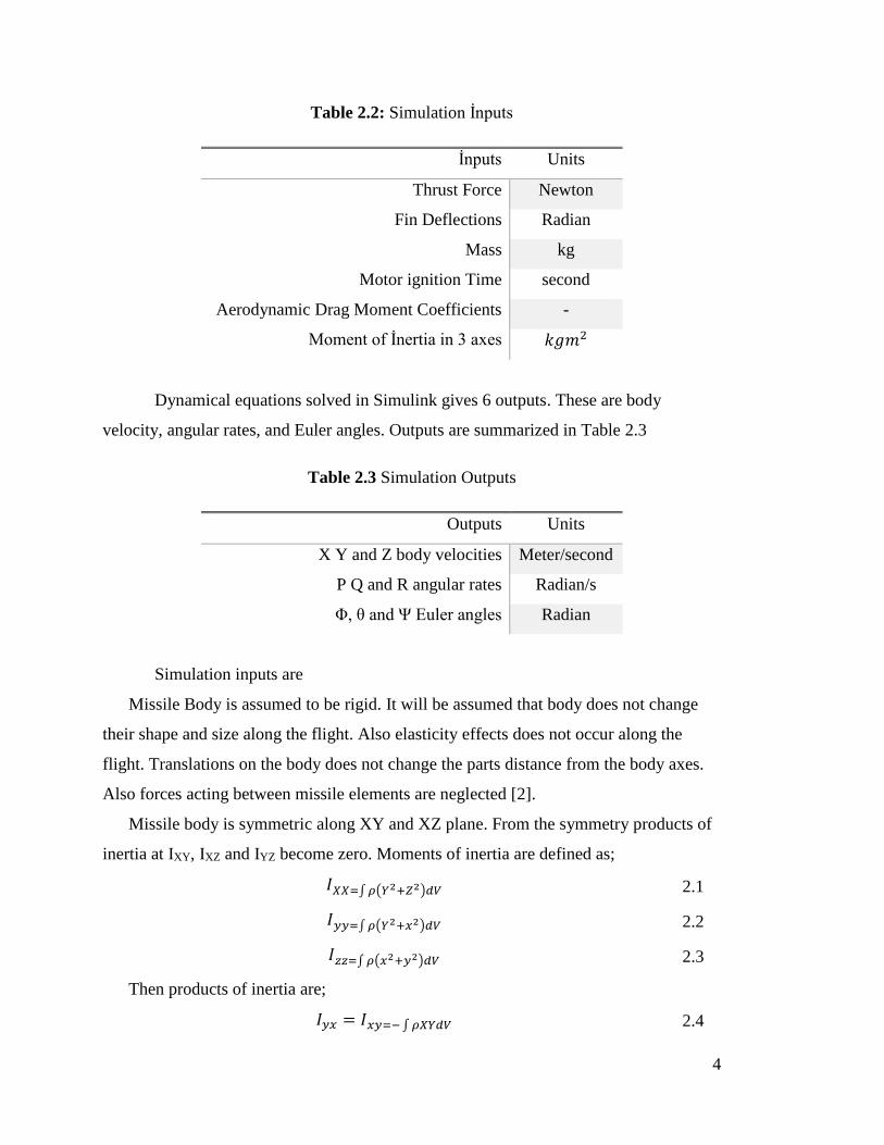
Table 2.2: Simulation İnputs

İnputs Units

Thrust Force Newton

Fin Deflections Radian

Mass kg

Motor ignition Time second

Aerodynamic Drag Moment Coefficients -

Moment of İnertia in 3 axes 𝑘𝑔𝑚2

Dynamical equations solved in Simulink gives 6 outputs. These are body

velocity, angular rates, and Euler angles. Outputs are summarized in Table 2.3

Table 2.3 Simulation Outputs

Outputs Units

X Y and Z body velocities Meter/second

P Q and R angular rates Radian/s

Φ, θ and Ψ Euler angles Radian

Simulation inputs are

Missile Body is assumed to be rigid. It will be assumed that body does not change

their shape and size along the flight. Also elasticity effects does not occur along the

flight. Translations on the body does not change the parts distance from the body axes.

Also forces acting between missile elements are neglected [2].

Missile body is symmetric along XY and XZ plane. From the symmetry products of

inertia at IXY, IXZ and IYZ become zero. Moments of inertia are defined as;

𝐼𝑋𝑋=∫ 𝜌(𝑌2+𝑍2)𝑑𝑉 2.1

𝐼𝑦𝑦=∫ 𝜌(𝑌2+𝑥2)𝑑𝑉 2.2

𝐼𝑧𝑧=∫ 𝜌(𝑥2+𝑦2)𝑑𝑉 2.3

Then products of inertia are;

𝐼𝑦𝑥 = 𝐼𝑥𝑦=− ∫ 𝜌𝑋𝑌𝑑𝑉 2.4

5

𝐼𝑥𝑧 = 𝐼𝑧𝑥=− ∫ 𝜌𝑋𝑍𝑑𝑉 2.5

𝐼𝑦𝑧 = 𝐼𝑧𝑦=− ∫ 𝜌𝑌𝑍𝑑𝑉 2.6

When integrating products of inertia, symmetry axes vanish each other and products

of inertial terms become zero [3].

Motor thrust just applied along +x axis. Missiles can be designed controllable

thrust to increase the maneuverability of missile. Thrust vectoring is not considered in

simulation model. Thrust is just applied along the x axis. Also thrust force vector is pass

from CM (center of mass).

Aerodynamic moments are applied from the CG (center of gravity).

Mass variation is assumed as linear. Initial mass, final mass and ignition time are

defined before the simulation. Algorithm create a mass matrix with respect to these 3

variable.

Figure 2.1 Missile axis Representation [2]

6

Aerodynamic cross-coupling terms are ignored. To simplify the equation, roll

motion terms inside the pitch and yaw motions are eliminated [2].

Counter clockwise is assumed as positive in both body axis and local reference

axis in simulation.

Air is incompressible during the flight. Also all aerodynamic coefficient are

assumed as constant along the flight. Missiles are generally flight over Mach 1. However

compressible aerodynamic calculations and effects are exceeds the scope of this study.

Earth is assumed as inertial reference system. Newton’s motion laws are written

in local Earth coordinate system. So rotation of earth around itself is ignored [3].

Moreover air is assumed as inviscid. No boundary layer occurs around missile body.

2.2. Missile Translational Equations

Missile movement assumed that has six degree of freedoms. 3 translational and 3

rotational degree of freedoms define the six degree of freedom. Translational and

rotational equations with respect to inertial frame can be expressed in the form;

∑ 𝐹 = 𝑚𝑎 2.7

∑ 𝑇 =𝑑

𝑑𝑡(𝑟 × 𝑚𝑉) 2.8

F is net force that is product of mass and acceleration. Net torque is T and it is derivative

of vector product of distance “r” and momentum “mV”.

Also this 2 equations can be expressed in terms of conservation of linear and

angular momentum with respect to the inertial frame. Equations become;

∑ 𝐹 =𝑑(𝑚𝑉𝑀)

𝑑𝑡 2.9

∑ 𝑀 =𝑑𝐻

𝑑𝑡 2.10

Six degree of dynamic equations can be rewritten in scalar form by using 3 force

and 3 moment. Force equations become;

7

𝐹𝑥 =𝑑(𝑚𝑢)

𝑑𝑡 𝐹𝑦 =

𝑑(𝑚𝑣)

𝑑𝑡 𝐹𝑧 =

𝑑(𝑚𝑤)

𝑑𝑡 2.11

Force components is mentioned in equation as u v and w that are respectively Vx

Vy and Vz. Moment equations also can expressed in the form;

𝐿𝑥 =𝑑𝐻𝑥

𝑑𝑡 𝐿𝑦 =

𝑑𝐻𝑦

𝑑𝑡 𝐿𝑧 =

𝑑𝐻𝑧

𝑑𝑡 2.12

L, M and N moments are called respectively, roll pitch and yaw moments. Hx Hy

and Hz are components of angular momentum. In the simulation setup, dynamical

equations are used in body frame. However equations that are mentioned in above are in

inertial frame. A vector in inertial frame can be expressed in body frame in the form;

(𝑑𝐴

𝑑𝑡)

𝑓𝑖𝑥𝑒𝑑= (

𝑑𝐴

𝑑𝑡)

𝑟𝑜𝑡𝑎𝑡𝑖𝑜𝑛𝑎𝑙+ 𝑤 × 𝐴 2.13

“A” is any vector and w is angular rates of rotational frame. So force equation can be

rewritten in body axes in the form;

(𝑑𝑉𝑀

𝑑𝑡)

𝑓𝑖𝑥𝑒𝑑= (

𝑑𝑉𝑀

𝑑𝑡)

𝑟𝑜𝑡𝑎𝑡𝑖𝑜𝑛𝑎𝑙+ 𝑤 × 𝑉𝑀 2.14

Second term in the right side of the equation is vector product of angular rates and

missile velocity. Vector product can be written as;

𝑤 × 𝑉𝑀 = (𝑖 𝑗 𝑘𝑃 𝑄 𝑅𝑢 𝑣 𝑤

) = (wQ − vR)i⃑ + (uR − wP)j⃑ + (vP − uQ)k⃑⃑ 2.15

P Q and R are respectively x y and z components of angular rates “w”. After the

implementation of rotational term in to the force equations, equations become;

∑ 𝐹𝑥 = 𝑚(�̇� + 𝑤𝑄 − 𝑣𝑅) 2.16

∑ 𝐹𝑦 = 𝑚(�̇� + 𝑢𝑅 − 𝑤𝑃) 2.17

∑ 𝐹𝑦 = 𝑚(�̇� + 𝑢𝑅 − 𝑤𝑃) 2.18

8

When this equation rewritten for derivative of u v and w;

du

dt= Rv − Qw + (

F𝑥

m) 2.19

dv

dt= Pw − Ru + (

F𝑦

m) 2.20

dw

dt= Qu − Pv + (

F𝑧

m) 2.21

Fx Fy and Fz forces are sum of thrust, drag forces, side forces and gravity force.

Thrust assumed just applied along +x direction in body frame.

Gravity acceleration is constant at inertial frame. Gravity acceleration vector at

inertial frame is;

[00

−𝑔] 2.22

Then gravity acceleration is multiplied with inertial to body acceleration matrix.

Coordinate transformation matrix will examined in following part of study. After that,

body axis gravity acceleration is obtained in the form;

𝑔 ∗ sin (𝜃)

−𝑔 ∗ sin(𝛷) ∗ cos (𝜃)

−𝑔 ∗ cos(𝛷) ∗ cos (𝜃) 2.23

These 3 terms will added to equations of translation respectively. So body acceleration

equations become;

du

dt= Rv − Qw + (

Thrust

m) + 𝑔sin (𝜃) 2.24

dv

dt= Pw − Ru + (

F𝑦

m) − 𝑔 sin(𝛷)cos (𝜃) 2.25

dw

dt= Qu − Pv + (

F𝑧

m) − 𝑔 cos(𝛷) cos (𝜃) 2.26

Aerodynamic force equations is built to add translational equations. Aerodynamic forces

expression is;

9

𝐴𝑒𝑟𝑜𝑑𝑦𝑛𝑎𝑚𝑖𝑐 𝑓𝑜𝑟𝑐𝑒 =1

2𝜌𝑉𝑚

2𝑆𝐶𝐷 2.27

ρ is air density, CD is drag coefficient, and S in reference area that is related with

calculated force side area. However this equation is written in wind axis frame. When

missile in maneuver situation, wind axis and body axis does not coincide. So drag force

equations should be written in body frame. To obtain body axis drag forces, forces will

multiplied with wind to body transformation matrix. Related transformation matrix

expressed as;

[

cos(𝛼) cos (𝛽) − cos(𝛼) sin (𝛽) −sin(𝛼)sin (𝛽) cos (𝛽) 0

sin(𝛼) cos(𝛽) − sin(𝛼) sin (𝛽) cos (𝛼)] 2.28

α is angle of attack and β is sideslip angle in this matrix representation. Transformation

matrix is expressed with “T”. Aerodynamic forces in related axis will be symbolized

with FAx FAy and FAz so body aerodynamic forces are;

𝐹𝐴𝑏= [𝑇𝑤

𝑏] × 𝐹𝐴𝑤 2.29

After adding the aerodynamic forces, translational equations can be expressed in this

from;

du

dt= Rv − Qw + (

Thrust

m) − g ∗ sin(θ) −

F𝐴𝑥

m 2.30

dv

dt= Pw − Ru + g ∗ cos(θ) ∗ sin(Φ) −

F𝐴𝑦

m 2.31

dw

dt= Qu − Pv + g ∗ cos(θ) ∗ cos(Φ) −

F𝐴𝑧

m 2.32

2.3. Missile Rotational Equations

Rotational equations generalized equations in inertial frame is expressed in the form;

∑ 𝑀 =𝑑𝐻

𝑑𝑡 2.33

10

Angular momentum H is expressed as;

�⃑⃑⃑� = 𝐼�⃑⃑⃑� 2.34

I is inertia matrix and w is angular velocity of body. İnertia matrix is written in matrix

form as;

𝐼 = [

𝐼𝑥𝑥 𝐼𝑥𝑦 𝐼𝑥𝑧

𝐼𝑦𝑥 𝐼𝑦𝑦 𝐼𝑦𝑧

𝐼𝑧𝑥 𝐼𝑧𝑦 𝐼𝑧𝑧

] 2.35

Angular momentum expression is also expressed in body frame. So equation should be

expressed in terms of inertial frame to add the body frame rotation inside to calculation.

(𝑑𝐻

𝑑𝑡)

𝑓𝑖𝑥𝑒𝑑= (

𝑑𝐻

𝑑𝑡)

𝑟𝑜𝑡𝑎𝑡𝑖𝑜𝑛𝑎𝑙+ 𝑤 × 𝐻 2.36

Vector product in second term of equation is;

𝑤 × 𝐻 = (

𝑖 𝑗 𝑘𝑃 𝑄 𝑅

𝐻𝑥 𝐻𝑦 𝐻𝑧

) = (𝐻𝑧Q − 𝐻𝑦R)i⃑ + (𝐻𝑥R − 𝐻𝑧P)j⃑ + (𝐻𝑦P − 𝐻𝑥Q)k⃑⃑ 2.37

Angular momentum H is expressed as cross product of ınertia matrix and angular

velocity. Derivative of angular momentum expression can be expanded as;

𝐼 × �̇� = [

𝐼𝑥𝑥 𝐼𝑥𝑦 𝐼𝑥𝑧

𝐼𝑦𝑥 𝐼𝑦𝑦 𝐼𝑦𝑧

𝐼𝑧𝑥 𝐼𝑧𝑦 𝐼𝑧𝑧

] [�̇��̇�

�̇�

] 2.38

Equation 2.38 also equals to;

= (𝐼𝑥𝑥�̇� + 𝐼𝑥𝑦�̇� + 𝐼𝑧𝑧�̇�)𝚤 + (𝐼𝑦𝑥�̇� + 𝐼𝑦𝑦�̇� + 𝐼𝑦𝑧�̇�)𝑗 + (𝐼𝑧𝑥�̇� + 𝐼𝑧𝑦�̇� + 𝐼𝑧𝑧�̇�)�⃑⃑� 2.39

In this study simulated aircrafts are assumed that they are symmetric along the xy

yz and xz plane. Inertia matrix become a diagonal matrix and expression simplified in

the form;

𝐻 = 𝐼 × 𝑤 = (𝐼𝑥𝑥�̇�)𝚤 + (𝐼𝑦𝑦�̇�)𝑗 + (𝐼𝑧𝑧�̇�)�⃑⃑� 2.40

Angular momentum is rewritten in the equation 1.9 as;

𝑤 × 𝐻 = (𝐼𝑧𝑧𝑅Q − 𝐼𝑦𝑦𝑄R)i⃑ + ((𝐼𝑥𝑥𝑃R − 𝐼𝑧𝑧𝑅P)j⃑ + (𝐼𝑦𝑦𝑄P − (𝐼𝑥𝑥𝑃Q)k⃑⃑ 2.41

11

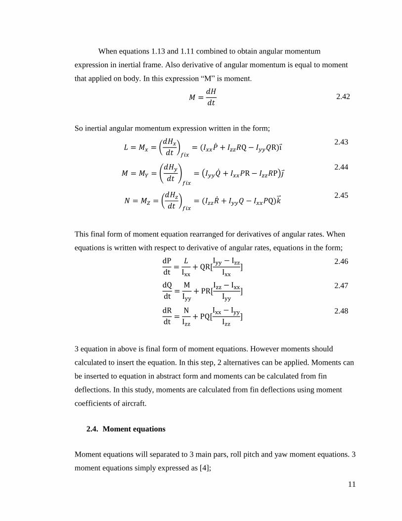
When equations 1.13 and 1.11 combined to obtain angular momentum

expression in inertial frame. Also derivative of angular momentum is equal to moment

that applied on body. In this expression “M” is moment.

𝑀 =𝑑𝐻

𝑑𝑡 2.42

So inertial angular momentum expression written in the form;

𝐿 = 𝑀𝑥 = (𝑑𝐻𝑥

𝑑𝑡)

𝑓𝑖𝑥= (𝐼𝑥𝑥�̇� + 𝐼𝑧𝑧𝑅Q − 𝐼𝑦𝑦𝑄R)i⃑

2.43

𝑀 = 𝑀𝑌 = (𝑑𝐻𝑦

𝑑𝑡)

𝑓𝑖𝑥

= (𝐼𝑦𝑦�̇� + 𝐼𝑥𝑥𝑃R − 𝐼𝑧𝑧𝑅P)𝑗 2.44

𝑁 = 𝑀𝑍 = (𝑑𝐻𝑧

𝑑𝑡)

𝑓𝑖𝑥= (𝐼𝑧𝑧�̇� + 𝐼𝑦𝑦𝑄 − 𝐼𝑥𝑥𝑃Q)�⃑⃑�

2.45

This final form of moment equation rearranged for derivatives of angular rates. When

equations is written with respect to derivative of angular rates, equations in the form;

dP

dt=

𝐿

Ixx+ QR[

Iyy − Izz

Ixx]

2.46

dQ

dt=

M

Iyy+ PR[

Izz − Ixx

Iyy]

2.47

dR

dt=

N

Izz+ PQ[

Ixx − Iyy

Izz]

2.48

3 equation in above is final form of moment equations. However moments should

calculated to insert the equation. In this step, 2 alternatives can be applied. Moments can

be inserted to equation in abstract form and moments can be calculated from fin

deflections. In this study, moments are calculated from fin deflections using moment

coefficients of aircraft.

2.4. Moment equations

Moment equations will separated to 3 main pars, roll pitch and yaw moment equations. 3

moment equations simply expressed as [4];

12

𝑀𝐴𝑦= 𝐿 = 𝐿𝑠𝑡𝑎𝑏𝑖𝑙𝑖𝑡𝑦 + 𝐹𝐴𝑌

(𝑧𝑐𝑔 − 𝑧𝑐𝑝) − 𝐹𝐴𝑍(𝑦𝑐𝑔 − 𝑦𝑐𝑝) 2.49

𝑀𝐴𝑦= 𝑀 = 𝑀𝑠𝑡𝑎𝑏𝑖𝑙𝑖𝑡𝑦 − 𝐹𝐴𝑌

(𝑧𝑐𝑔 − 𝑧𝑐𝑝) + 𝐹𝐴𝑍(𝑥𝑐𝑔 − 𝑥𝑐𝑝) 2.50

𝑀𝐴𝑧= 𝑁 = 𝑁𝑠𝑡𝑎𝑏𝑖𝑙𝑖𝑡𝑦 + 𝐹𝐴𝑌

(𝑦𝑐𝑔 − 𝑦𝑐𝑝) − 𝐹𝐴𝑍(𝑥𝑐𝑔 − 𝑥𝑐𝑝) 2.51

These equations consist of 3 parts. First term include the fin deflections stability

and moment coefficients. Second and third terms are become effective when missile

center of pressure (CP) and center of mass (CM) is placed different coordinates in

related axes.

To calculate the L M and N axes stability moments, terms should be derive from

the aerodynamic coefficients. In the definition of roll, pitch and yaw moment, δ wil be

used for control surface deflection. Roll, pitch and yaw control surface deflections will

be symbolized as δr δp and δy. Stability coefficients are functions of different flight

parameters. Moment and drag coefficients can be determined experimentally or

numerically with complex algorithms. Moment coefficients are function of;

𝐶 = 𝐶(𝛼, 𝛽, �̇�, �̇�, 𝑀𝑛, δ𝑟 , δ𝑝, 𝛿𝑦, 𝑢, 𝑣, 𝑤, 𝑝, 𝑞, 𝑟) 2.52

Calculation of aerodynamic coefficients is not covered in this study. Coefficients are

founded from related works to use in calculation. Stability moment equations is

expressed as [4];

𝐿𝑠𝑡𝑎𝑏𝑖𝑙𝑖𝑡𝑦 = 𝑄𝑆𝑑𝐶𝑙 2.53

𝑀𝑠𝑡𝑎𝑏𝑖𝑙𝑖𝑡𝑦 = 𝑄𝑆𝑑𝐶𝑚 2.54

𝑁𝑠𝑡𝑎𝑏𝑖𝑙𝑖𝑡𝑦 = 𝑄𝑆𝑑𝐶𝑛 2.55

S is reference area of missile in related plane. d is reference length and generally

used as body diameter of missile. 𝑄 is dynamic pressure that is also used in drag

calculations.

Related aerodynamic moment coefficients that include the damping terms are

modeled as [4];

𝐶𝑙 = 𝐶𝑙𝛿𝛿𝑟 + (

𝑑

2𝑉𝑀)𝐶𝑙𝑃

𝑃 2.56

13

𝐶𝑚 = 𝐶𝑚𝛼𝛼 + 𝐶𝑚𝛿

𝛿𝑝 + (𝑑

2𝑉𝑀) (𝐶𝑚𝑞

+ 𝐶𝑚�̇�) 𝑞

2.57

𝐶𝑛 = 𝐶𝑛𝛽𝛽 + 𝐶𝑛𝛿

𝛿𝑦 + (𝑑

2𝑉𝑀) (𝐶𝑛𝑟

+ 𝐶𝑛�̇�) 𝑟

2.58

𝛿𝑟 is fin deflection for roll movement, 𝛿𝑝 fin deflection for pitch angle and 𝛿𝑦 fin

deflection for yaw maneuver. Study does not aim to concern with aerodynamic

coefficients. Because of the fact 𝐶𝑚�̇�and 𝐶𝑛�̇�

coefficients are combined with 𝐶𝑚𝑞

and 𝐶𝑛𝑟. Rearranged equations simplify the simulation to obtain stable missile.

Expressed moment coefficient are placed to the moment equation and equation

becomes in the form of;

𝐿𝑠𝑡𝑎𝑏𝑖𝑙𝑖𝑡𝑦 = 𝑄𝑆𝑑 [𝐶𝑙𝛿𝛿𝑟 + (

𝑑

2𝑉𝑀)𝐶𝑙𝑃

𝑃] 2.59

𝑀𝑠𝑡𝑎𝑏𝑖𝑙𝑖𝑡𝑦 = 𝑄𝑆𝑑 [𝐶𝑚𝛼𝛼 + 𝐶𝑚𝛿

𝛿𝑝 + (𝑑

2𝑉𝑀) (𝐶𝑚𝑞

+ 𝐶𝑚�̇�) 𝑄]

2.60

𝑁𝑠𝑡𝑎𝑏𝑖𝑙𝑖𝑡𝑦 = 𝑄𝑆𝑑 [𝐶𝑛𝛽𝛽 + 𝐶𝑛𝛿

𝛿𝑦 + (𝑑

2𝑉𝑀) (𝐶𝑛𝑟

+ 𝐶𝑛�̇�) 𝑅]

2.61

Moment equations placed in the angular rates equation and final from of angular

rates equation written as;

dP

dt=

𝑄𝑆𝑑 [𝐶𝑙𝛿𝛿𝑟 + (

𝑑2𝑉𝑀

)𝐶𝑙𝑃𝑃]

Ixx+ QR [

Iyy − Izz

Ixx]

2.62

dQ

dt=

𝑄𝑆𝑑 [𝐶𝑚𝛼𝛼 + 𝐶𝑚𝛿

𝛿𝑝 + (𝑑

2𝑉𝑀) (𝐶𝑚𝑞

+ 𝐶𝑚�̇�) 𝑄]

Iyy+ PR [

Izz − Ixx

Iyy]

2.63

dR

dt=

𝑄𝑆𝑑 [𝐶𝑛𝛽𝛽 + 𝐶𝑛𝛿

𝛿𝑦 + (𝑑

2𝑉𝑀) (𝐶𝑛𝑟

+ 𝐶𝑛�̇�) 𝑅]

Izz+ PQ [

Ixx − Iyy

Izz]

2.64

Now considering the 3 translation equations that eq x,x and 3 rotational equation

on above we obtain six equations for our six degree of freedom simulation. As it is clear

that these six equations are highly nonlinear. However solving these six equations

numerically gives body velocity and body angular rates of simulated missile.

14

2.5. Coordinate Frame Transformations

Dynamical equations that are used in simulation is built in body frame. However

some terms in the equations is easier to define in other reference systems these are

aerodynamic forces and gravity acceleration. After the defining these terms, it converted

in to the body frame to insert to dynamical equations derived in previous chapters.

2.5.1. Wind to Body Transformation Matrix

In maneuvering condition, aerodynamic side forces occur on the body of missile.

Aerodynamic forces equations are written in wind axis system. Difference between the

wind axis and body axis is created with angle of attack (α) and side slip angle (β).

Transformation matrix can be created with help of this 2 angle. 3 body axis is written in

the form of wind axis components. Components of body axis on wind axis shown at

Figure 2.2 .

Figure 2.2 Wind Axis System [2]

15

Using current angle of attack and side slip angle at every time step in simulation,

wind to body axis transformation matrix created as;

[

cos(𝛼) cos (𝛽) − cos(𝛼) sin (𝛽) −sin(𝛼)sin (𝛽) cos (𝛽) 0

sin(𝛼) cos(𝛽) − sin(𝛼) sin (𝛽) cos (𝛼)] 2.65

2.5.2. Inertial to Body Transformation Matrix

Gravity acceleration is constant and in the direction of –z direction in inertial

frame. So it should be transformed in to the body frame to insert into translational

equation. Using Euler angles, inertial to body transformation matrix expressed as;

[

cos(𝜃) cos (𝛹) cos(𝜃) sin (𝛹) −sin (𝜃)

sin(𝛷) sin(𝜃) cos(𝛹) − cos(𝛷) sin (𝛹) sin(𝛷) sin(𝜃)sin (𝛹) + cos(𝛷) cos (𝛹) sin(𝛷) cos (𝜃)

cos(𝛷) sin(𝜃) cos(𝛹) + sin(𝛷) sin (𝛹) cos(𝛷) sin(𝜃) sin(𝛹) − sin (𝛷)𝑐𝑜𝑠(𝛹) cos(𝛷) cos (𝜃)

] 2.66

Roll angle is expressed with psi “Φ”. Pitch angle is symbolized with theta (θ) and

yaw is shown with psi (Ψ). Building the transformation matrix is not considered in this

study. However angles show the difference between the inertial and body axes. Then

transformation matrix created considering the projection of transformed vectors.

Body to inertial transformation matrix is used to obtain inertial displacement of

missile and it is equal to inverse of inertial to body matrix. Transformation matrices are

orthogonal. So transpose of inertial to body matrix gives inverse transformation matrix.

Transformation applied to body axes data and simulation result obtained in any desired

reference frame.

Transformation matrix changes with roll, pitch and yaw angle at every time step.

To obtain current transformation matrix, roll pitch and yaw angles should be obtained in

every time step in simulation. Derivative form of Euler angles Roll Pitch and Yaw

respectively [3].

𝑑𝛷

𝑑𝑡= 𝑃 + (

𝑑𝛹

𝑑𝑡) ∗ 𝑠𝑖𝑛𝜃

2.67

𝑑𝜃

𝑑𝑡= 𝑄 ∗ 𝑐𝑜𝑠𝛷 − 𝑅 ∗ 𝑠𝑖𝑛𝛷

2.68

16

𝑑𝛹

𝑑𝑡= (𝑄 ∗ 𝑠𝑖𝑛𝛷 + 𝑅 ∗ 𝑐𝑜𝑠𝛷)/𝑐𝑜𝑠𝜃

2.69

Equations 2.67, 2.68 and 2.69 are also solved numerically along the simulation

to obtain current Euler angles. Using Euler angles transformation matrix are updated at

every time step. However at +90 degree and -90 degree pitch angles, yaw angles become

infinite because of the zero division. To negotiate this problem, different kind of

algorithms can be used. Also different kind of rotation parameters can be used to

measure the rotations such as quaternions or Rodrigues parameters. In this study,

simulation is built with Euler angles. Simulation is tested under the limited pitch angle

conditions.

17

3. SENSOR FUSION USING VIRTUAL SENSOR

3.1. Purpose

Simulation results are flawless. However real data obtained from missiles

includes noise and resolution limits. Using MATLAB Sensor Fusion Toolbox, simulated

model data are processed to obtain realistic sensor data. A missile model needs a

controller for guidance and navigation. Study looks an answer for what Sensor Fusion

Toolbox is sufficient or not for navigation part of a missile design. In this study İMU

(Inertial Measurement Unit) and GPS sensor will be used. İMU sensor includes

accelerometer, gyroscope and magnetometer sensors. İMU and GPS sensor data are

fused to make a better prediction of orientation and position of missile. Estimated

positions and orientations compared with non-fused sensor data and simulated model

data. Estimation performance are compared.

3.2. IMU Sensor Model

IMU sensor created in MATLAB is include accelerometer, gyroscope and

magnetometer. IMU sensor parameters can be configured. IMU sensor input are given in

local coordinate system. Inputs are orientation, angular velocity and local to body

rotation matrix. Outputs of IMU sensor are accelerometer readings, gyroscope readings

and magnetometer readings in 3 dimensions. Units of input parameter are meter over

Second Square for acceleration data and radian per second for gyroscope data.

Magnetometer data are in unit of micro Tesla. [5]

An important point while using IMU sensor object, sensor object adds

gravitational acceleration on input data. Simulation data that obtained in this study also

include the gravitational acceleration. Before the analyzing data, additional gravitational

acceleration should be subtracted from related axis. NED (North-East-Down) axis is

used in sensors. So related axis is z axis.

18

3.3. GPS Sensor Model

GPS sensor object models data input to obtain realistic GPS sensor data.

Horizontal and vertical position accuracy, velocity accuracy decay factor and sample

rate parameters are defined before using the object. GPS sensor inputs are position and

velocity in local navigation coordinate system. Units of inputs are respectively meter and

meter over second. Outputs of GPS sensor are position, velocity, ground speed and

course data. Ground speed data is magnitude of horizontal velocity. Course data is

direction of groundspeed vector. Position data are given in Latitude-Longitude and

Altitude (LLA) coordinate system. Also reference location is determined before using

GPS sensor object, because distances are change in LLA coordinate system with respect

to reference location. [5]

3.4. IMU and GPS Model Fusion

Missiles are very fast aircrafts and estimation of position and orientation is an

important process for guidance of missile. To obtain better estimation of position and

orientation of aircraft, different sensor’s data are used together. MATLAB Sensor

Fusion Toolbox include estimation filters to process the sensor data. In this study,

insfilterMARG object that is included in Sensor Fusion Toolbox is used to fuse sensor

data. InsfilterMARG object use Extended Kalman filter to make a prediction and

correction.

Extended Kalman filter use 22 state to make a prediction. These are respectively,

4 quaternions, 3 positions, 3 velocity, 3 gyroscope bias, 3 accelerometer bias, 3

geomagnetic field vector and 3 magnetometer biases. 22 state are used to create a

position estimation. Mathematical background of Extended Kalman filter is not covered

in this study.

3 object function are used in position and orientation estimation. First function

predict states using acceleration and gyroscope data. Second function fuse GPS data.

Then third function fuse magnetometer data. Accelerometer and gyroscope frequencies

are much higher than GPS and Magnetometer readings. GPS sensor sample rate is used

19

as sample per second. At every second, estimations are made by using only IMU data.

After 1 second, states are updated with GPS and magnetometer measurements.

3.5. Results

İn this study six degree of freedom of a missile model and realistic sensor navigation

results are computed and presented. Missile simulation results compared with MATLAB

6DOF block. Therefore correctness of dynamical equations are checked. NED axes

positions and orientation data are compared. 15 km altitude sounding rocket is simulated

for navigation study.

Simulated missile physical properties are summarized in Table 3.1

Table 3.1 Missile Physical Properties

Missile Physical Properties Property Unit

Missile Length 3 Meter

Missile Diameter 0.15 Meter

Missile Center of pressure 2.39 Meter

Mass at initial 33 Kg

Mass after burnout 15 Kg

Motor Thrust 600 Newton

Missile center of gravity is change with time depend with motor burn time. It is assumed

that motor ignition and mass decreasing is linear along the motor burn. During the

simulation to obtain lateral displacement, 0.4 radian fin deflection is applied along 2.5

second. Fin deflection is started at 20 second on simulation. Position in NED

coordinates, Euler angles in Radians and body velocity that are obtained from simulation

are shown in Figure 3.1 NED Position of Missile Simulation Position and velocity unit is

used as meter.

20

Figure 3.1 NED Position of Missile Simulation

Body axes velocity of missile is shown in Figure 3.2.

Figure 3.3 Body Axes Acceleration of Missile

Figure 3.2 Body Velocity of Missile

21

Body axes acceleration of missile during simulation are shown in Figure 3.3

Roll pitch and yaw Euler angles are shown in Figure 3.4. Figure 3.1, 3.2 and 3.3

shows that missile gives clear response to fin deflections. Missile aerodynamic stability

is enough at experienced fin deflection. Maximum acceleration is 20 m/s along the

flight. Exact match is obtained at result between simulation and MATLAB Simulink

6DOF block. After the simulation, simulated data are processed in virtual sensor.

Euler angles figure shows that after the apogee, missile is turning their around

during the free fall. Also we can observe that after the fin deflection at second 20, yaw

angles pull back with a small angle. Because of the main velocity vector is in the altitude

direction at 20 second, it is an expected result. After obtaining missile simulation results,

next step is sensor simulation results.

As a first sensor parameters are defined. After setup the parameters, sensor

fusion algorithm estimate the position and orientation of aircraft. Accelerometer,

gyroscope, magnetometer and GPS data are used to obtain missile flight estimation.

Missile flight simulation and sensor estimation altitude data are shown in Figure 3.5.

Figure 3.4 Roll pitch and Yaw angles along the flight

22

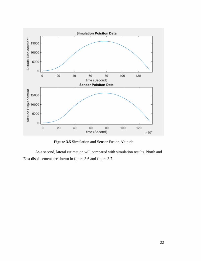
Figure 3.5 Simulation and Sensor Fusion Altitude

As a second, lateral estimation will compared with simulation results. North and

East displacement are shown in figure 3.6 and figure 3.7.

23

Figure 3.7 Simulation and Sensor Fusion results at North direction

Figure 3.6 Simulation and Sensor Fusion Results at East direction

24

It is an important point that East direction displacement fluctuations are

expected. Because of there is no displacement at east direction on the simulation, sensor

estimation fluctuations shown more clear than altitude and North directions.

After the calculation, it is observed that sensor estimations accuracy is changes

up to 500 meters at large displacement coordinates. Difference between the simulation

and sensor estimations in NED coordinate system is shown in figure 3.8

3.6. Future Works

Results of this study shows that MATLAB Sensor Fusion Toolbox

algorithms can be used for estimation of sounding rockets controller design.

However accuracy of estimations should be considered with respect to operation

Figure 3.8 Estimation errors at NED coordinates

25

requirements. High maneuvers conditions and different sensor parameter results

are not considered in this study. As a future work extended Kalman filter states

can be applied without using MATLAB functions to decrease the computational

time.

Extended Kalman filters are used for state estimation using states

matrices and previous data. In this study, state matrix created using the relation

of sensor parameters between them. Relations are written in matrix from. All the

sensor parameters and noise parameters are used in this matrix to predict the next

data at each time step. For example cruise missiles use this to prediction to find

their position and orientation in real time. So controller can decide the necessary

control input. Therefore improving the estimation algorithm play an important

role on navigation and guidance of missiles.

26

4. CONCLUSION AND RECOMMENDATIONS

Six degree of freedom simulation of a missile and realistic sensor navigation results

are presented in this study. MATLAB sensor Fusion Toolbox is used to create realistic

sensor data. Also an estimation filter that is presented in Sensor Fusion Toolbox is used

to fuse obtained sensor data. Missile flight simulation is created in MATLAB Simulink.

Fundamental mathematical blocks are used for calculations. Three translational

equations and three rotational equations are used to calculate missile body in every time

step. Thrust force, current mass, and fin deflections are inputs of simulation. Position

and orientation with respect to local coordinate system, angular rates are output of

simulation. Motor initial and final mass are defined before simulation. Also missile

body, nosecone and fin side areas are used to calculate center of pressure of missile.

Moment and forces are calculated in body frame. Moment equations include 8 moment

coefficients. Three of them used to calculate the fin deflections effect at three rotational

axes. Other three set of moment coefficients are used to define angular rate effects on

moments. Last two moment coefficients are used calculate to pitch and yaw angle

effects on moments. After simulation results are compared with MATLAB 6DOF block.

Almost perfect match is obtained between simulation results and 6DOF block results.

Secondly, obtained results from simulation environment, processed in

MATLAB Sensor Fusion Toolbox using virtual sensors. Virtual sensors take necessary

data and add noise and disturbances to create a realistic sensor data. When creating

realistic data, use sensor parameters that are defined before process. İn this study IMU

and GPS sensors are used to create sensor data. After that, an estimation filters are used

to obtain more accurate position and orientation data. Estimation filters are tried under

different sensor sample rates and results are presented. It is observed that increasing

IMU sample rate gives better estimation despite low sample rate GPS data. Altitude

estimation with Sensor Fusion Toolbox gives relatively high accuracy data with respect

the horizontal axes estimations.

In conclusion, creating a simulation environment and using navigation estimation

for missiles are examined in this study. Sensor estimations for missile flight are fused

using MATLAB algorithms and accuracy results are presented.

27

REFERENCES

[1] S. Steinkellner, "Aircraft Vehicle Systems Modeling and," Linköpıng Studies In

Science And Tecnology, p. 3, June 2011.

[2] G. M. Sıourıs, "Aerodynamic Forces and Coefficients," in Missile Guidance and

Control Systems, New York, Springer, 2004.

[3] P. N. Jenkins, "Missile Dynamics Equations for Guidance," US Army Missile

Laboratory, Redstone Arsenal, 1984.

[4] S. S. Wibowo, "Full envelope six-degree of freedom simulation of tactical missile,"

in AIP Publishing, 2020.

[5] The MathWorks Inc., "MathWorks Documentation," The MathWorks Inc.,

[Online]. Available: https://www.mathworks.com/help/nav/ref/gpssensor-system-

object.html. [Accessed 24 01 2021].