Master thesis Dimitry Brons, s1460447

Graduation assignment IEM: Maintenance Planning at Twente Milieu.

Supervisor: Dr. E. Topan

Second supervisor: Dr. I. Seyran Topan

Company supervisor: R. de Kruijff

Version: 07/10/19

Preface This thesis marks the end of my life as an Industrial Engineering and Management student at

the University of Twente. During the past years I have learned more than I could ever imagine

when entering the university as a freshman in 2013.

I want to thank Twente Milieu and especially Ruben de Kruijff for the opportunity and the

freedom they gave me to conduct this research on maintenance management of underground

bins. My gratitude also goes to my colleagues Remco, Ewald and Annika who were always

there to answer my questions about Twente Milieu and underground bin management.

Secondly, I want to thank my university supervisors Engin and Ipek Topan who always

managed to find time to guide me in the right direction and give me valuable feedback to

continue my research.

Thirdly, I would like to express my sincere gratitude to my parents and Robin and Quirine for

always making me feel more than welcome back home in Ermelo and supporting me

unconditionally. Due to them every weekend I could spend in Ermelo was enjoyable and gave

me the motivation to finish my studies in Enschede.

And lastly I want thank everyone who made studying in Enschede such a great pleasure. De

Eetclub, Darshana and Linda for all joyful moments spent together, all my Arriba teammates

during the past seasons for so many good games and practices and all other people at Arriba

who made my time at Arriba unforgettable.

Dimitry Brons, Enschede, October 2019

Management summary The public grounds management department of Twente Milieu maintains the underground

bins in Twente by correctively repairing bins that fail due to several reasons. There are two

types of corrective repair, (i) first line maintenance for failures in the electronics or above the

ground and (ii) second line maintenance for failures in the mechanics of the bin for which the

bin has to be lifted out the pit. Besides the corrective repairs, Twente Milieu hires an external

company to carry out preventive maintenance to each underground bin twice a year.

Preventive maintenance contains the washing, lubrication and inspection of the underground

bin on the bin site.

Twente Milieu has the desire to insource preventive maintenance. This research seeks to add

a preventive maintenance policy to the current corrective maintenance policy for maintaining

underground bins. The introduction of preventive maintenance gives the opportunity to

employ the mechanics at Startpunt, the name of the workshop in Borne.

The introduction of preventive maintenance at Startpunt has other projected advantages over

the current situation. Firstly, money that is paid to an external company is invested in their

own mechanics, who are educated at the same time. Secondly, the quality of the maintenance

improves since the bins are maintained in a workshop instead of on the street. Thirdly, after

the outsourced preventive maintenance Twente Milieu receives an inspection report which

might lead to corrective repairs. Therefore, second line mechanics need to go to the bin site

and carry out the repair, which requires extra movements. The number of these movements

can be decreased by carrying out preventive maintenance at Startpunt and repair all errors at

the same time.

From the current situation analysis we concluded that a lot of bins are visited at least once a

year for corrective repair by either the first line or the second line mechanics. A visit can be

used to repair the bin correctively and simultaneously as an opportunity to carry out

preventive maintenance.

By conducting a literature review on maintenance management we found out that the failure

distribution is an indicator of the effectiveness of preventive maintenance. There are two

failure distributions that are commonly used in maintenance management; the exponential

distribution for random failures and the Weibull distribution for wear out failures. Based on

the failure distribution, the optimal preventive maintenance can be determined. To

incorporate decisions based on events, we decided to carry out a discrete event simulation

study as well.

To differentiate between maintenance methods, we consider four policies. (i) Corrective

repair at the bin site, (ii) corrective replacement of a broken bin by a repaired bin from stock,

(iii) age-based preventive replacement of an active bin by a repaired bin and (iv) opportunistic

maintenance when a bin breaks down. Opportunistic maintenance in this case means using

the opportunity of a failure of one bin, to give preventive maintenance to another bin that is

active in the neighbourhood.

The failure distribution for underground bins is determinant for an effective preventive

maintenance policy. To find the failure distribution we carried out a data analysis on the failure

data. By looking at the time between failures of an underground bin, we found out that there

are two relevant failure distributions. The failure distribution for first line failures which is

exponentially distribution and the failure distribution for second line failures which is Weibull

distributed with a value of β larger than 1. For this reason we concluded that preventive

maintenance will only be effective for second line mechanics, consequently we leave the first

line mechanics out of the scope for this research.

The failure distribution is the main input of the cost function maintenance planning model.

The cost function shows that the effectiveness of an age-based preventive maintenance policy

is strongly dependent on the costs for corrective and preventive maintenance.

The next step in this research is the incorporation of costs for downtime, making decisions

based on events and opportunistic maintenance. We decided to carry out a discrete event

simulation study to see what gains we can get from using the ability to respond to failures

according to maintenance policies.

To optimize the maintenance policy we considered three input variables; (i) the weekly

capacity of Startpunt, (ii) the preventive maintenance interval and (iii) a threshold of a number

of days before bins are allowed to be repaired at Startpunt. The preventive maintenance

threshold in the simulation study is introduced to determine a minimum time a bin has to be

on the street before it is allowed to get preventive maintenance at Startpunt again. Failures

before this threshold time are repaired on bin site. The results of the simulation study are

measured in total costs for the maintenance strategy, the average downtime of bins and the

number of maintenance actions by second line mechanics.

The simulation study shows that a shorter preventive maintenance interval leads to lower

costs and a lower downtime, but to a lot of variability in the times bins are on the street. The

variability is a measure to determine the average number of days between two instances of

preventive maintenance intervals at Startpunt and the variance of this average. A higher

preventive maintenance threshold contributes to the higher variability as well. The higher

threshold leads to bins that are allowed to go to Startpunt earlier, which increases the

deviation in the average time between two preventive maintenance instances. The increased

variability is a negative consequence of such a strategy.

The desire to decrease the variability leads to an investigation on using a preventive

maintenance interval of 365 days instead of 240 days. The goal is to have an average time

between two preventive maintenance instances at Startpunt of around 365 days with a

smaller variance. Using longer preventive maintenance results in costs that are higher than in

the previous scenario, but leads to lower variability in the time between two preventive

maintenance instances. The main advantage of the decreased variability is that the average

time on the street of all bins is about the same, which makes it easier to stick to a maintenance

planning, since the preventive maintenance planning becomes less responsive to failures

occurring all through the municipality.

From the results of the simulation study based on the Hengelo case, we advise Twente milieu

to start insourcing preventive maintenance activities to Startpunt on the bins in the

municipality Hengelo with a preventive maintenance interval of one year and apply a

preventive maintenance threshold of 90 days. These settings lead to improvement regarding

costs, reduction of downtime and reduction of second line maintenance actions, compared to

the current situation with outsourced preventive maintenance. In the near future, this process

can be started by hiring the transportation truck and figuring out the capacity of Startpunt and

how many bins can be transported on one day. This information can be used to assess the

possibilities to scale up this maintenance policy to the underground bins in Enschede and the

rest of Twente.

vi

Index Preface ......................................................................................................................................................ii

Management summary ........................................................................................................................... iii

Terminology ............................................................................................................................................. ix

List of Figures ............................................................................................................................................ x

List of Tables ............................................................................................................................................ xi

1. Introduction ..................................................................................................................................... 1

1.1 Twente Milieu .......................................................................................................................... 1

1.2 Research motivation ................................................................................................................ 1

1.3 Research goal .......................................................................................................................... 2

1.4 Scope ....................................................................................................................................... 2

1.5 Research questions.................................................................................................................. 3

2. Current situation and desired situation .......................................................................................... 5

2.1 Waste collection ...................................................................................................................... 5

2.1.1 Differentiated fees .......................................................................................................... 5

2.1.2 Public bins ........................................................................................................................ 5

2.1.3 Composition of an underground bin ............................................................................... 6

2.2 Maintenance methods ............................................................................................................ 8

2.2.1 Information systems ........................................................................................................ 8

2.2.2 Corrective maintenance .................................................................................................. 9

2.2.3 Consequences of downtime .......................................................................................... 10

2.2.4 Preventive maintenance................................................................................................ 11

2.3 Maintenance in numbers ...................................................................................................... 11

2.4 Desired Situation ................................................................................................................... 13

2.4.1 Advantages of the desired situation ............................................................................. 14

2.4.2 Constraints of the desired situations ............................................................................ 14

2.5 Washing, lubrication and inspection at Startpunt ................................................................ 16

2.6 Case Hengelo ......................................................................................................................... 17

2.7 Conclusions ............................................................................................................................ 18

3. Literature review on maintenance methods ................................................................................. 19

3.1 Maintenance methods .......................................................................................................... 19

3.1.1 Preventive maintenance concepts ................................................................................ 19

Time-based maintenance .............................................................................................................. 20

Usage-based maintenance ............................................................................................................ 20

Usage-severity-based maintenance .............................................................................................. 20

vii

Condition-based maintenance ...................................................................................................... 21

3.2 Failure distributions ............................................................................................................... 21

Exponential distribution ................................................................................................................ 22

Weibull distribution ....................................................................................................................... 22

Chi square test ............................................................................................................................... 23

3.3 Opportunistic maintenance ................................................................................................... 24

3.4 Discrete event simulation ...................................................................................................... 24

Advantage of a simulation study over real-life experiments ........................................................ 25

Advantages of a simulation study over other modelling approaches ........................................... 25

Disadvantages of a simulation study ............................................................................................. 25

3.5 Conceptual model ................................................................................................................. 26

3.6 Experimentation .................................................................................................................... 26

Warm-up period ............................................................................................................................ 26

Number of replications .................................................................................................................. 27

3.7 Relevance to this research .................................................................................................... 28

4. Modelling approach ...................................................................................................................... 29

4.1 Maintenance methods .......................................................................................................... 29

4.2 Research outline .................................................................................................................... 30

4.3 Age-based maintenance ........................................................................................................ 31

4.4 Discrete event simulation ...................................................................................................... 31

4.4.1 Opportunistic maintenance in the simulation model ................................................... 32

4.4.2 Conceptual model ......................................................................................................... 32

4.4.3 Assumptions, simplifications and verification ...................................................................... 37

4.5 Conclusions of the modelling approach ................................................................................ 38

5. Numerical analysis ......................................................................................................................... 39

5.1 Failure data ............................................................................................................................ 39

5.1.1 Method of data gathering ............................................................................................. 39

5.1.2 Life time distributions .................................................................................................... 40

5.1.3 Discussion on data analysis ........................................................................................... 43

5.2 Numerical analysis for time-based preventive maintenance ................................................ 43

5.2.1 Costs for preventive and corrective maintenance ........................................................ 43

5.2.2 Discussion on maintenance interval .............................................................................. 45

5.3 Numerical analysis for discrete event simulation ................................................................. 47

5.3.1 KPI’s ............................................................................................................................... 47

5.3.2 Warm-up period ............................................................................................................ 48

5.3.3 Input variables and hypotheses .................................................................................... 49

viii

5.3.4 Experimental design ...................................................................................................... 50

5.3.5 Results ........................................................................................................................... 50

5.4 Validation .............................................................................................................................. 56

5.5 Sensitivity analysis ................................................................................................................. 56

5.6 Conclusions of the numerical analysis .................................................................................. 58

6. Conclusions and recommendations .............................................................................................. 60

6.1 Conclusions ............................................................................................................................ 60

6.2 Recommendations for Implementation ................................................................................ 61

6.3 Recommendations for further research ................................................................................ 62

6.4 Contribution to literature and practice ................................................................................. 63

References ............................................................................................................................................. 64

Appendix A Flowchart conceptual model ......................................................................................... 65

Appendix B Decision chart maintenance engineer ........................................................................... 66

Appendix C Table of the Chi-square test .......................................................................................... 67

Appendix D Simulation results with maintenance interval of 365 days ........................................... 68

ix

Terminology AWRS System that communicates about the status of underground bins. For example, about

how full the bin is, which is measured by the number of bags dropped into the bin, the

level of the battery and the number of times it has been opened and by who.

KCC System used by the customer service to communicate civilian complaints about

underground bins to the maintenance department.

Wincar System to keep track of the maintenance history of the underground bins. Work orders

for all activities are booked in this system.

Webfleet System to keep track of all trucks driving around. The TomTom route planner is part of

this system which is present in every Twente Milieu truck.

Diftar Differentiated fees for customers to dispose their waste. Based on the principle: “user

pays”. If one disposes more waste, he must pay more disposal fees.

BOR Public ground management; this department of Twente Milieu is responsible for the

management of all public grounds in the municipalities.

MU Moving unit, term in simulation model for a unit that moves through the system.

KPI Key performance indicator.

Startpunt Name of the workshop in Borne, where working and education is combined.

BWaste Manufacturer of underground bins, company who carries out washing and lubrication

in current situation and supplier of electronics for card readers and AWRS.

x

List of Figures Figure 1 Underground bin ....................................................................................................................... 6

Figure 2 Smart box with card reader ....................................................................................................... 7

Figure 3, Current process for corrective maintenance ......................................................................... 10

Figure 4 Illegal disposal of garbage bags ............................................................................................... 11

Figure 5 Maintenance activities per year .............................................................................................. 13

Figure 6 Histogram of the numbers of visits per underground bin per year ........................................ 13

Figure 7, Process of bin replacement for preventive maintenance at Startpunt.................................. 15

Figure 8 Desired process of washing, lubrication and inspection at Startpunt .................................... 17

Figure 9 Bathtub curve .......................................................................................................................... 20

Figure 10 Time based vs usage based life time distribution ................................................................. 21

Figure 11 Types of maintenance ........................................................................................................... 30

Figure 12 Black box model of the discrete event simulation study ...................................................... 34

Figure 13 explanation of threshold for preventive maintenance ......................................................... 35

Figure 14 Histogram of times to failure of first line failures ................................................................. 41

Figure 15 Histogram of times to failure of second line failures ............................................................ 41

Figure 16 cost function G(T) .................................................................................................................. 45

Figure 17, Dashboard of the discrete event simulation model ............................................................. 47

Figure 18 MSER output .......................................................................................................................... 48

Figure 19 Results of the second simulation run .................................................................................... 52

Figure 20 Average time on the street against preventive maintenance interval ................................. 53

Figure 21 Average time on the street against capacity at Startpunt. ................................................... 54

Figure 22 Results of the sensitivity analysis based on different cost parameters ................................ 57

xi

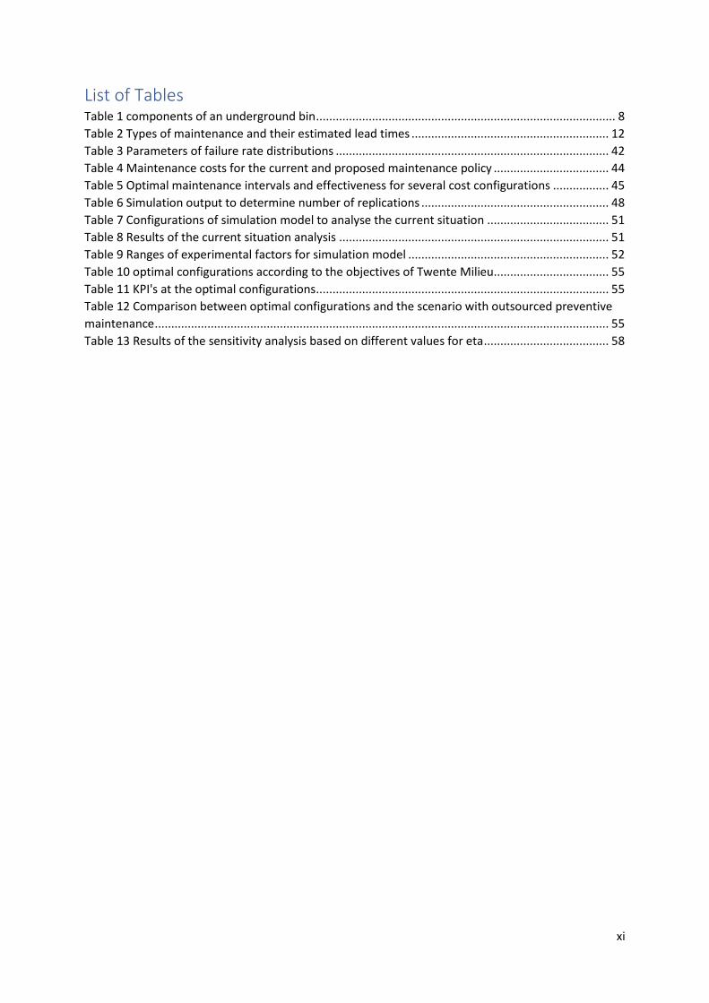
List of Tables Table 1 components of an underground bin ........................................................................................... 8

Table 2 Types of maintenance and their estimated lead times ............................................................ 12

Table 3 Parameters of failure rate distributions ................................................................................... 42

Table 4 Maintenance costs for the current and proposed maintenance policy ................................... 44

Table 5 Optimal maintenance intervals and effectiveness for several cost configurations ................. 45

Table 6 Simulation output to determine number of replications ......................................................... 48

Table 7 Configurations of simulation model to analyse the current situation ..................................... 51

Table 8 Results of the current situation analysis .................................................................................. 51

Table 9 Ranges of experimental factors for simulation model ............................................................. 52

Table 10 optimal configurations according to the objectives of Twente Milieu................................... 55

Table 11 KPI's at the optimal configurations ......................................................................................... 55

Table 12 Comparison between optimal configurations and the scenario with outsourced preventive

maintenance .......................................................................................................................................... 55

Table 13 Results of the sensitivity analysis based on different values for eta ...................................... 58

1

1. Introduction In this report, we execute a research on maintenance management of the underground bins at

Twente Milieu. Section 1.1 introduces the company Twente Milieu. Section 1.2 gives reasons

why this research is carried out at Twente Milieu. Chapter 1.3 defines the goal of the research.

Section 1.4 explains the scope of this research. Section 1.5 states the research questions.

1.1 Twente Milieu Twente Milieu collects the waste of the citizens in eight municipalities in Twente. Besides this,

Twente Milieu is responsible for managing public grounds such as greenery in towns,

preventing slippery roads and maintaining the sewage system. Besides these responsibilities

on public grounds, the company owns five workshops to carry out maintenance activities on

their trucks, machinery and public bins. These workshops are located in Enschede, Hengelo,

Almelo, Oldenzaal and Borne.

The company was founded in 1997 when the waste collectors of Enschede, Almelo, Hengelo

and Oldenzaal started working together to collect the waste. For a short period of time, the

company was a mixed owned company with 35% of the shares were sold to a private company.

In 2005 the municipalities got all shares back and Twente Milieu became a government

company with their shares divided over eight municipalities in Twente. This means that

Twente Milieu is commissioned by the municipalities and follows the waste and public

grounds policy of the different municipalities.

The managing team on public grounds (BOR) is responsible for the maintenance of the public

bins around the municipalities of Twente Milieu. The management of the underground bins is

divided over three divisions. The placing department who is responsible for placing the

underground bins in the street. This job includes digging a pit, transporting and installing the

bin and assuring the street is repaired by an external company. The maintenance department

is responsible for the coordination and execution of the maintenance teams on the street

throughout the day. The workshop department is responsible for assembling new

underground bins and repairing underground bins in one of the workshops of Twente Milieu.

These repairs include mainly painting and welding, which cannot be carried out at the bin

location.

1.2 Research motivation The main maintenance activities of Twente Milieu are mainly in response to notifications by

customers or waste collectors and are therefore corrective. For preventive maintenance

Twente Milieu has a service contract with a company called BWaste which performs

preventive maintenance actions (washing, inspection and lubrication) on every underground

bin twice a year.

The current contract for preventive maintenance results in poor insights in the state of the

underground bins. Besides this, the preventive maintenance is carried out at the bin location,

and could possibly be done more thoroughly by insourcing the preventive maintenance

activities. The BOR department has the desire to insource the preventive maintenance

activities. The start of this process is scheduled in 2019 with a pilot by insourcing preventive

2

maintenance on the underground bins in the municipality Hengelo. In this pilot, all

underground bins are considered.

The three main reasons for Twente Milieu to insource preventive maintenance are as follows.

In the first place to extend the life cycle of the underground bins by carrying out the preventive

maintenance activities more thoroughly at workshops. In the second place, to give Twente

Milieu better opportunities to keep track of the status of their assets. The third reason is that

the amount of jobs for the employees at Startpunt is decreasing. In order to generate work

for these employees, a social project of labour and education can continue which has great

social value for Twente Milieu.

This research seeks to optimize the preventive maintenance process to be insourced by

Twente Milieu. Preventive maintenance includes washing, lubricating and inspecting the

underground bins at called Startpunt. Chapter 2 elaborates on this process.

1.3 Research goal The goal of the research is to optimize the preventive maintenance process for underground

bins at Twente Milieu by designing a maintenance model for Twente Milieu that includes

corrective and preventive maintenance. The maintenance model should include a new

process of preventive maintenance (washing, lubrication and inspection at Startpunt) and

insourcing preventive maintenance needs to fit within the available capacity of Startpunt. In

order to reach this goal, there are two sub goals, firstly to identify all relevant processes in the

new situation after insourcing preventive maintenance, and secondly, to identify the relevant

costs, constraints, failure distributions and opportunities. The findings of the two sub goals

are combined into a maintenance planning of the underground bins in the municipalities of

Twente.

1.4 Scope Although Twente Milieu works in many different fields in order to manage the public grounds

of the municipalities in Twente, this research focusses on the maintenance activities carried

out at the public bin locations and at Startpunt. Only Startpunt is considered, since this

workshop plays a key role in the maintenance of underground bins.

The scope of this research is the tactical level of the maintenance planning. During this

research, some assumptions may be used about actions that not have been realized by Twente

Milieu yet but are likely to happen in (near) future. Furthermore, routing is not in the scope

of this research, so estimations about driving time between undergrounds will be rough.

In the past, Twente Milieu has had different suppliers for underground bins, due to the

obligation to have public tenders. These different suppliers deliver different types of

underground bins with different frameworks. Since the lifetime of an underground bin is

longer than the time between these tenders, various types of bins are used. Not all bins are

yet suitable for the proposed way of maintenance, so this research focusses only on the

suitable bins of which the number is likely to rise in the future, which increases the practical

use of this research.

3

1.5 Research questions The main research question is: How can Twente Milieu optimize the preventive maintenance

process of washing, lubricating and inspection of their underground bins?

To answer the main research question, the following sub questions are defined:

1. What is the current situation concerning corrective and preventive maintenance?

i. What are the current processes at Twente Milieu?

ii. What is the current approach for corrective maintenance?

iii. What is the current approach for preventive maintenance?

iv. What data is available to analyse the current situation?

v. How to use this data to measure current performance?

Section 2.1 to 2.3 describe the current situation at Twente Milieu and give a brief description

of waste collection in general, an explanation of the process of corrective maintenance, and

an overview of the current preventive maintenance strategy. The sub questions concern the

performance of the current maintenance strategies, both preventive and corrective.

2. How does the desired situation for Twente Milieu look like?

i. What are the objectives of desired situation?

ii. What are the constraints on the desired situation?

iii. How is the desired situation influenced by the constraints by Twente Milieu?

Section 2.4 and 2.5 and describe the desired situation by Twente Milieu, namely to carry out

the preventive maintenance by themselves. This requires insight into the opportunities and

constraints of the desired situation.

3. Which methods can be found in literature about maintenance optimization and which

are applicable to the case at Twente Milieu?

i. What is the advantage of preventive maintenance?

ii. What kind of preventive maintenance policies exist?

iii. How can failure distributions be characterized?

iv. What is opportunistic maintenance?

v. How can discrete event simulation be used in this research?

Chapter 3 provides an overview of ideas and existing solutions in the literature. The results of

this literature study can be used as a basis to design a solution for the research problem stated

in chapter 1.

4

4. What approaches can we use to model and optimize the maintenance policy of Twente

Milieu?

i. What maintenance methods should we incorporate in the maintenance

model?

ii. What does a maintenance planning model for age-based maintenance look

like?

iii. What is the conceptual model for a discrete event simulation study for

optimizing maintenance at Twente Milieu?

Chapter 4 builds on the ideas found in literature and presented in chapter 3. These ideas are

used to develop an analytical maintenance planning model and a discrete event simulation

model. Chapter 4 describes four maintenance (section 4.1) methods and how the

maintenance methods are incorporated in the age-based maintenance planning model

(section 4.3) and the discrete event simulation model (section 4.4).

5. What maintenance strategy optimizes maintenance in such a way that it fits within the

capacity of Startpunt and includes more variability?

i. What is the failure distribution that can be used in the proposed maintenance

models?

ii. What are the numerical results of using a time-based preventive maintenance

strategy?

iii. What are the results of the discrete event simulation study to implement the

proposed maintenance methods at Twente Milieu?

Chapter 5 gives a numerical analysis on the two models described in chapter 4. The

parameters for the failure distribution must be determined before analysing the model

(section 5.1). Section 5.2 uses the failure distribution to show the use of working with a

preventive maintenance interval. Section 5.3 extends the study with a discrete event

simulation model, to analyse the variability in the proposed maintenance policy.

Chapter 6 states the main conclusions of this research and provides recommendations to

Twente Milieu.

5

2. Current situation and desired situation Chapter 2 describes the context of the research at Twente Milieu. Section 2.1 explains the way

of collecting waste in the municipalities in Twente and we elaborate more on the main assets

of this research, the public bins. Section 2.2 elaborates on the current maintenance methods

and policy. Section 2.3 quantifies the current corrective maintenance strategy. Section 2.4

gives insight in how the desired situation for Twente Milieu looks like. We zoom into the

process at Startpunt in section 2.5. Section 2.6 describes why we use Hengelo as a case study.

Section 2.7 explains the conclusions that we can draw from the current and desired situation.

2.1 Waste collection The waste collection in the municipalities served by Twente Milieu is done by different means

and according to different policies in the municipalities. In the following sections the main way

of waste collection will be discussed.

In order to dispose their waste, inhabitants of the municipalities fill three large bins (240 L),

with residual waste, with paper waste and with bio waste. These bins are put along the streets

on a biweekly basis. On these collection days, truck drivers from Twente Milieu empty the

bins. The civilians pay a standardized fee for each time their residual waste bin is emptied,

whereas the bio waste and paper waste bins are emptied for free.

These three bins are still used by a part of the inhabitants and Twente Milieu still collects the

waste in these bins. However, the waste collection is shifting towards public underground bins

located everywhere throughout the municipality, where inhabitants drop their waste in bags

of 30 L.

2.1.1 Differentiated fees

Over the last two decades, more municipalities started to use differentiated fees (Diftar) for

the collected waste. Consequently civilians have an incentive to reduce their waste and

separate residuals better, thus lowering waste deposit costs. Over the years this strategy has

contributed to a better separation of waste streams by civilians with a reduction in residual

waste of 25% from 2016 to 2017 (Gemeente Enschede, 2019). The separation of public waste

streams leads to partly filled bins along the roads or bins that are offered less frequently along

the roads. In the future, Twente Milieu aims at collecting all waste via public bins, and thus

abolishing the 240 L private bins.

2.1.2 Public bins

To give inhabitants the opportunity to dispose their separated waste streams such as glass

and textile, public bins are installed at several places in the municipalities. The disposal of

waste via these underground bins is free. Inhabitants still pay for the disposal of residual waste

against a fee of €0,84 per bag of 30 L. Since the separation of waste streams leads to smaller

amounts of residual waste, civilians start to dispose their residual waste more and more often

in public bins where they pay per bag of residual waste they offer (Gemeente Enschede, 2019)

instead of using their 240 L bin. These underground bins are widely available in the

municipalities so all citizens have the opportunity to dispose their waste close to their home.

6

The municipalities do not have enough room in the infrastructure to have all bins above the

ground so technologies have been developed to store the waste under streets and sidewalks

in underground bins. In figure 1 we can see such an underground bin, which has a small area

above the surface and a rather large (3-5 cubic meters) underground storage.

Twente Milieu has installed over 2500 underground bins in eight municipalities in the region

of Twente (Twente Milieu, 2015). These underground bins are available to the citizens with a

registered municipal environmental card. The containers are meant to collect paper, glass,

residual, textile and packages to stimulate a secure separation of waste.

2.1.3 Composition of an underground bin

This section describes the underground bin and explains which components need

maintenance. The underground bin has a black part above the ground and grey container are

underground (Figure 1). On top of the bin, a carrying shaft is attached to the hull.

The black hull with an input slot that can be opened for waste streams with free disposal e.g.

textile and glass. Besides, these slots can also be covered by a grey trommel as shown in figure

1, which allows the user to dispose just one bag of 30 L when it opens.

Inside the hull, an electric lock makes sure the trommel can only be opened once per card that

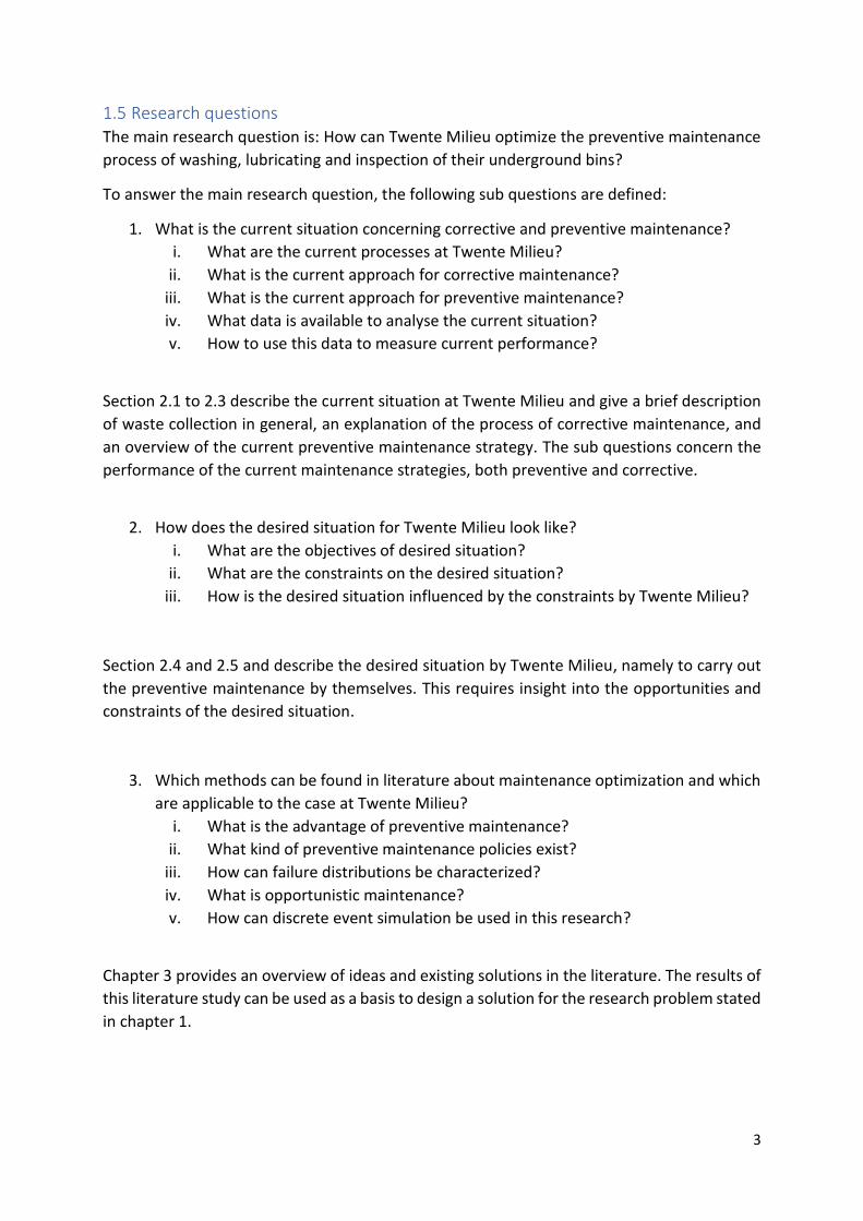
is presented. There is also an electronic device with a card reader (figure 2), a memory and a

data connection with the server. This smart box is used to register each bag dropped, open

the lock when a valid card is presented and send daily the data to the server. The software

that is used by this smart box is called Administrative Waste Registration System (AWRS).

Figure 1 Underground bin

7

Outside the hull, a carrying shaft is attached to chains inside the bin. A crane pulls up the

underground bin by using the carrying shaft and then opens the bottom of the bin above a

waste truck. Table 1 summarizes the relevant components.

Administrative Waste Registration System (AWRS) AWRS is the remote monitoring system that communicates the status of the underground bin

to Twente Milieu. In the first place, it registers the number of garbage bags dropped in a bin,

so it knows how full an underground bin is at any time. How full it is, is given as a percentage

of the maximum number of bags in can take namely: 𝐹𝑢𝑙𝑙𝑛𝑒𝑠𝑠 = 𝑁𝑢𝑚𝑏𝑒𝑟 𝑜𝑓 𝑑𝑟𝑜𝑝𝑝𝑒𝑑 𝑏𝑎𝑔𝑠

𝑀𝑎𝑥𝑖𝑚𝑢𝑚 𝑛𝑢𝑚𝑏𝑒𝑟 𝑜𝑓 𝑏𝑎𝑔𝑠∗

100%. Secondly it sends a report with the current battery statuses every night, so a dead

battery can be quickly identified as a possible cause for problems. The AWRS also registers

who opened the bin for the last time to drop a garbage bag. AWRS is also used to verify if

problems have been resolved. For example, if one user makes a notification of a stuck bin, and

another resolves the problem howsoever Twente Milieu knows the problem has been

resolved since more garbage droppings have occurred after the first stuck notification.

Figure 2 Smart box with card reader

8

Table 1 components of an underground bin

List of components Function

Hull Part of the bin that is above the ground. The hull contains an input slot for waste in the size suitable for the waste stream.

Smart box

The card reader that communicates with the server. After reading a presented valid card, it makes sure the lock opens and the trommel can make one rotation to take in one bag. The smart box registers the card number of the customer in order to make him pay to Twente Milieu. It can also read if a card is valid and stay closed for an invalid card. Lastly, every night, the smart box sends its data to a server so the maintenance department can read the data.

Trommel The trommel closes the input slot of paid waste streams. The trommel is large enough to carry one 30 L garbage bag.

Lock The lock can be opened by the smart box in order to make the trommel rotate once. This means that the trommel opens, the customer can drop one bag and the trommel closes again.

Battery The battery is attached inside of the hull in order to give power to the lock and the smart box. When the battery is dead, it is replaced by a new one. Every night a battery status is sent to the server by the smart box.

Carrying shaft On top of the bin, there is a carrying shaft so a crane can pull the underground bin out of the pit and empty it in the garbage truck.

Chains The chains are attached to the carrying shaft and make sure the bottom of the underground bin can open to drop the waste into the garbage truck.

2.2 Maintenance methods This section describes the information systems at Twente Milieu which are used for

underground bin management. Secondly, the maintenance methods for the underground bins

are described. There are two types of maintenance activities applied to underground bins:

corrective maintenance which is carried out by mechanics of Twente Milieu and preventive

maintenance which is outsourced to a company called BWaste.

2.2.1 Information systems

Real-time data is used to manage the maintenance. The main advantage of this is that the

maintenance department decides upfront whether it is necessary to send mechanics to the

underground bin or that the problem is caused by a customer because of a wrong or outdated

card, for example. In the latter case, the failure is not in the bin itself, so the maintenance

team is not necessary. The customer service and the customer with the failing card should

seek for a solution together. This aspect is not taken into account in this research.

Customer contact centre (KCC) Customer contact centre (KCC) is the information system by which the customer service communicates a civilian complaint or notification to the maintenance department. The maintenance department uses their other systems to check if there is a real problem and how to fit the underground bin in the maintenance schedule. Wincar Wincar is the information system where Twente Milieu registers the working hours of the

mechanics on the road and at the workshops. In addition, a history of all maintenance actions

to underground bins is registered in Wincar.

9

Routing programs There are several programs used for routing purposes: Webfleet, TomTom, AWRS, and

Garmin. Twente Milieu uses Webfleet including TomTom to keep track of their trucks during

the day and to give the mechanics the possibility to navigate to a location. All bin locations are

connected in AWRS and TomTom. In addition, a Garmin tool is used to optimize routes via

multiple locations.

2.2.2 Corrective maintenance

Corrective maintenance is carried out by Twente Milieu in response to civilian complaints,

notifications or waste collectors or digital warnings. Corrective maintenance can be above or

below the ground and is carried out by two different departments called first line (above the

ground) and second line (underground). These departments have their own car or truck, which

is their working space.

Both lines drive all working days around in the municipalities and, they carry out (i) planned

jobs which occurred overnight or the day before and (ii) respond to problems that occur during

the day at one or more of the bins. The second line can lift the underground bin out of the

ground by means of a crane and solve any problems with the pit or the frame of the bin. A

frequently occurring problems for the second line are broken frames or a smelly air around

the bins, because of the dirty pit. The first line can only solve problems concerning the

electronics or the outside hull of the bins. Their main tasks are the replacement of batteries,

card readers and locks. Besides this, they repair bins where garbage bags got stuck due to

various causes.

The maintenance department plans corrective maintenance as immediate as possible to

reduce downtime as much as possible. However, in most cases the corrective maintenance is

postponed a few hours, which gives time to check AWRS to look into the bin data. The bin

data check concerns what has happened to the underground bin in the time span between

the failure notification and the moment the mechanics leave. They check when the bin has

opened correctly for the last time, the last time it registered a customer card and how full the

bin is. By this data, the maintenance department assesses the type of failure and send the

right mechanics (first or second line).

If it is clear that no check is needed, the failure is sent to the first or second line immediately,

which can go to the bin and repair immediately. This practice is a response to many

unnecessary maintenance trips in the past and facilitated by the availability of real-time data

from smart card readers.

The flowchart in figure 3 shows the corrective maintenance process and which departments

are responsible for what part. This flowchart shows how Twente Milieu executes corrective

repairs on a daily basis.

10

Figure 3, Current process for corrective maintenance

2.2.3 Consequences of downtime

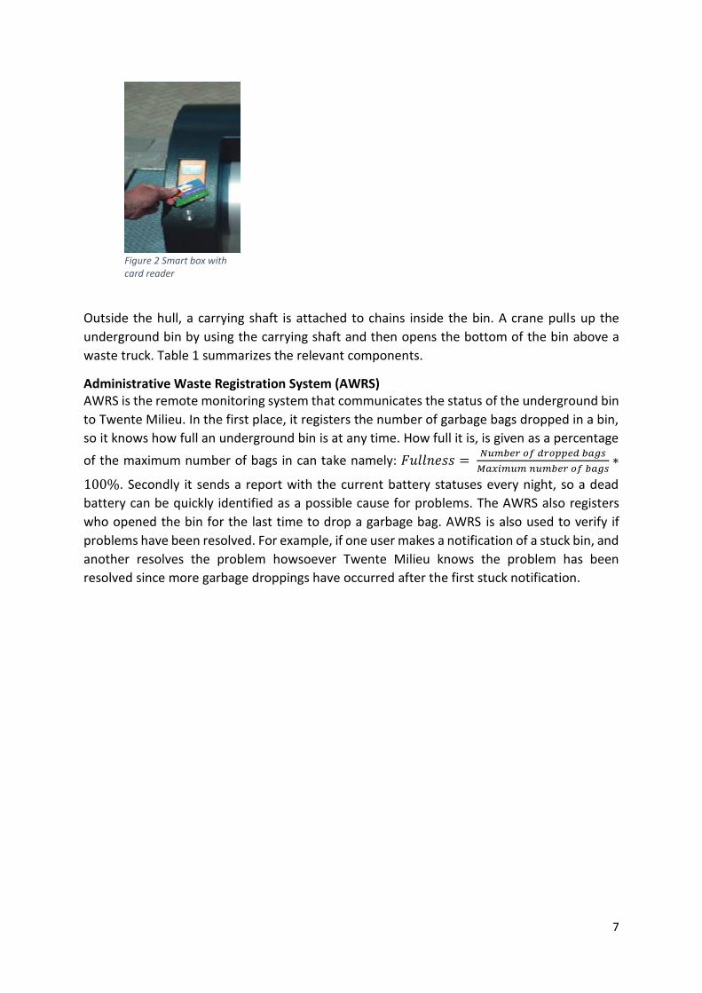
It is important to keep downtime of underground bins as short as possible. Downtime is

defined as the time where customers cannot dispose their waste in an underground bin. Too

much downtime results in negative experiences for customers, neighbourhood inhabitants

and lost revenues for Twente Milieu. With non-functioning bins, frequently people do not take

their garbage back home but leave their garbage around the underground bin and do not pay

for disposing waste and create a mess on public grounds as displayed in figure 4. For these

reasons, it is important that failures are adequately resolved by both the first line and second

line mechanics.

11

Figure 4 Illegal disposal of garbage bags

2.2.4 Preventive maintenance

As mentioned before, Twente Milieu has a service contract with BWaste who cleans the

underground bins twice a year. Bin are cleaned at location with a high-pressure cleaner and

by lubricating the bins with penetrating oil. , BWaste also cleans the pit to minimize smelly airs

around the bins. Twente Milieu receives an inspection report about this preventive

maintenance including the status of the underground bin. Twente Milieu pays BWaste €42,50

per container per year to carry out the described preventive maintenance activities.

The result of the activities by BWaste is a list of small issues or deficits for every bin cleaned

by BWaste. These issues are in most cases resolved by second line mechanics of Twente

Milieu, who can just like BWaste carry the bin out of the pit and repair minor issues.

2.3 Maintenance in numbers This section seeks to quantify the current situation in terms of corrective and preventive

maintenance by assessing how many work orders on corrective repairs are fulfilled by first-

and second-line mechanics in a year. The data is obtained from Wincar (Twente Milieu, 2015),

the internal work order system of Twente Milieu. For each task related to a public bin the

mechanics make a work order with a specification of the maintenance carried out.

Five kinds of corrective maintenance activities are taken into account and specification follows

of the kind of failure, its cause and the specific maintenance activity:

Corrective repairs: Maintenance after customer notification. These failures are mainly input

slots that get stuck by the insertion of too large garbage bags. These maintenance actions

normally do not take very long.

Vandalism maintenance: Maintenance that occurs from vandalism, for example, graffiti or

demolishment of the input slots. These maintenance actions usually take somewhat longer

because metals might need repair or the underground bin needs some paint or thorough

washing with a high-pressure cleaner.

External digital maintenance: This includes all maintenance on the electronic parts of the

underground bin. The electronic parts are the card reader and the battery which gives power

to the lock and input slot. It is considered external since the costs for these repairs are paid by

BWaste instead of Twente Milieu. The lead time for this kind of repairs depends on the age of

12

the underground bin. For some bins, just a few screws are enough to carry out the

maintenance, while for other bins, the whole electronic system needs to be unscrewed.

External corrective repairs: All repairs of non-electronic parts of the underground bins. These

maintenance actions have different lead times.

Internal damage: This category is corrective repairs carried out on failures caused by the

material handling by Twente Milieu workers. These failures are most often in the larger part

of the underground bin, for example in the shaft to which the crane connects. Dents due to

collisions between the crane and the underground bin is another example of internal damage.

These damages often concern the metal frames or shaft and usually, the lead times for repair

is long.

Table 2 Types of maintenance and their estimated lead times

Type of maintenance Operator Repair lead time

Corrective maintenance First or second line differs for line and job

Vandalism maintenance First or second line about 0.5 hour

External digital maintenance First line about 0.25 hour

External corrective maintenance Second line Over 2 hours

Internal damage Second line Long

Table 2 summarizes the maintenance methods, with the operating lines and estimated lead

times. The rough estimations are based on the bookings for maintenance methods that

include a large variety of jobs and execution times.

The number of corrective maintenance carried out has increased over the past years (Figure

5 and 6). This is due to two trends. The first trend is the increased number of underground

bins in the streets and more municipalities being served by Twente Milieu. The second trend

is the fact that internal damages are being monitored more securely, so there is more data

available on what kinds of maintenance have been carried out.

An interesting mark in figure 5 is that large corrective maintenance activities which are

internal damages and vandalism. These failures occur about 500 times per year as shown in

figure 5.

13

Figure 5 Maintenance activities per year

Figure 6 shows the frequency of visits per underground bin per year. The bins that are never

visited are not shown, because this would generate an unbalanced dataset. Over 1600

underground bins are visited for corrective maintenance at least once in 2018, this is the sum

of the bins that are visited once, twice, three times etc. These visits for corrective maintenance

give opportunities for inspection or preventive maintenance. In addition, there is an

opportunity for a full preventive maintenance treatment of washing, lubricating and

inspection instead of activating the first- or second-line truck for corrective maintenance.

Figure 6 Histogram of the numbers of visits per underground bin per year

2.4 Desired Situation This section explains the desired situation by Twente Milieu. The desired situation concerns

the carrying out of preventive maintenance at the workshops of Twente Milieu, including

washing, lubricating and inspecting the bin. The starting point for preventive maintenance is

that every underground bin is regularly brought in a workshop.

0

1000

2000

3000

4000

5000

6000

2015 2016 2017 2018

Number of maintenance activities per year

External corrective maintenance

Vandalism

Internal damage

External digital maintenance

Corrective maintenance

0

100

200

300

400

500

600

1 2 3 4 5 6 7 8 9 10 11 12 13 14

2015 2016 2017 2018

14

Startpunt in Borne is the chosen workshop, primarily because this workshop has a social

importance. Twente Milieu seeks to employ people with a distance to the labour marked in

combination with technical schooling at the ROC school in Hengelo. By insourcing the

preventive maintenance, money spent on washing, lubrication and inspection of the

underground bins are invested in Twente Milieu labour instead of external labour.

In the current situation, Twente Milieu uses Startpunt only to assemble underground bins. The

underground bins are delivered as raw materials and the mechanics assemble them to

complete underground bins. However, the number of assembly jobs is decreasing, so using

the workshop space and mechanics to carry out preventive maintenance is an opportunity to

generate work for Startpunt.

Besides preventive maintenance at the workshop, the container might need to be more

frequently washed on the street. This depends on the wishes of the municipality where the

underground bins are located.

2.4.1 Advantages of the desired situation

In the end situation, each underground bin in a municipality in the service area of Twente

Milieu can be replaced by any other washed, lubricated and inspected underground bin from

the stock at Startpunt. During a replacement, the framework in the ground and the pit must

be cleaned as well, which job is done BWaste during their washing round in the current

situation.

An additional advantage of carrying out preventive maintenance at Startpunt instead of at bin

location is the improved quality of preventive maintenance. According to the estimations of

mechanics, the underground bins are as good as new after they are treated at Startpunt. This

is better than in the current situation since the on-site preventive maintenance is not as

thorough as it could be at Startpunt.

2.4.2 Constraints of the desired situations

The most important constraint is the working capacity of Startpunt. Since the employees are

being taught and still going to school, the working hours are restricted to school hours and

holidays. In addition, the capacity is influenced by the number of newly arriving employees

who need more instructions at the beginning of their period of employment and can work

more independently and faster towards the end of their employment period.

Another constraint to the current situation is that not all frameworks of the underground bins

are the same. This means that not all containers are interchangeable as described in the

advantages in section 2.3.1. It is unsure when all frameworks will be uniform and a way should

be found to deal with this problem.

It is also necessary that a bin for a certain waste stream is replaced by a bin of the same waste

stream. So another constraint for the desired situation is that there are sufficient bins of all

waste streams in stock to replace bins in the street that need washing, lubrication and

inspection.

15

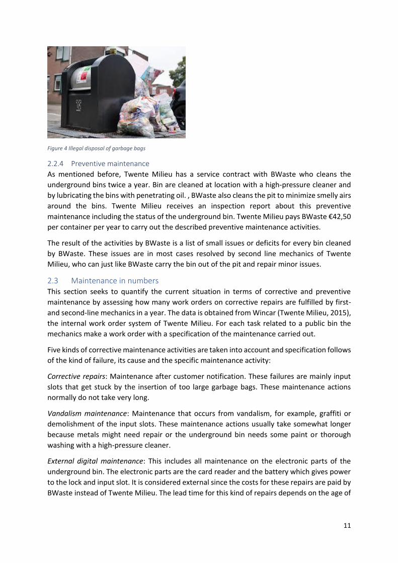
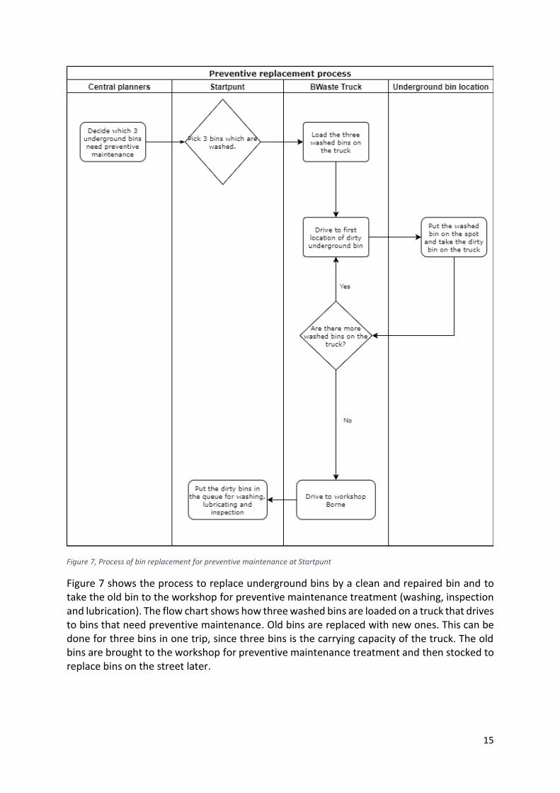
Figure 7, Process of bin replacement for preventive maintenance at Startpunt

Figure 7 shows the process to replace underground bins by a clean and repaired bin and to take the old bin to the workshop for preventive maintenance treatment (washing, inspection and lubrication). The flow chart shows how three washed bins are loaded on a truck that drives to bins that need preventive maintenance. Old bins are replaced with new ones. This can be done for three bins in one trip, since three bins is the carrying capacity of the truck. The old bins are brought to the workshop for preventive maintenance treatment and then stocked to replace bins on the street later.

16

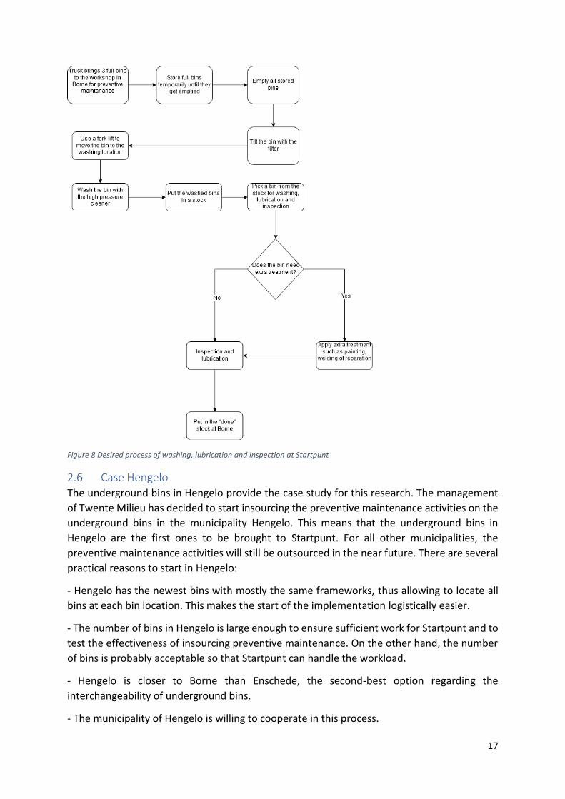
2.5 Washing, lubrication and inspection at Startpunt Chapter 1 mentioned the great social value of Startpunt. This section elaborates on this social

value and explains the preventive maintenance actions in the form of washing, lubrication and

inspection which are going to be carried out by the employees of Startpunt. Insourcing the

process of washing, lubrication and inspection to Borne is a way to ensure that there is enough

work at Startpunt to warrant capacity for the working and learning environment.

At Startpunt employees work from October up to and including July for four days a week. The

fifth day is reserved for theoretic and practical schooling. The area of the workshop is designed

in such a way that there is enough space to store the underground bins. The underground bins

come (partly) filled with garbage from the street in batches of at most three bins because of

the truck capacity. The bins arrive only on days that the truck is hired, this day we label

transportation day. Theoretically the truck can be hired any working day, but this would

involve high costs because of daily payment for truck rent.

The bins must be emptied from garbage before they treatment at the workshop. Emptying a

bin is done with a crane and a garbage truck which is open on top. After bins are emptied, the

crane puts them on a tilting frame, because the bins can only be moved horizontally with a

forklift.

There is a special part of the terrain reserved for washing with a high-pressure cleaner.

Washing a bin is one of the least time-consuming activities of the process. The capacity of the

wash area in bins per hour is much larger than the capacity of the rest of the process. After

washing bins are stored and it is assessed which treatments are needed. Some bins might be

in a very good state and need only penetrating oil, while other bins might need a new layer of

paint or need to be welded.

After the additional treatment, bins are lubricated with penetrating oil and a final inspection

follows. Bins are inspected by using a checklist and then brought to the done bin’s storage.

From this storage, bins can be taken immediately to put on the streets. Figure 8 shows a

flowchart of the process described above.

17

Figure 8 Desired process of washing, lubrication and inspection at Startpunt

2.6 Case Hengelo The underground bins in Hengelo provide the case study for this research. The management

of Twente Milieu has decided to start insourcing the preventive maintenance activities on the

underground bins in the municipality Hengelo. This means that the underground bins in

Hengelo are the first ones to be brought to Startpunt. For all other municipalities, the

preventive maintenance activities will still be outsourced in the near future. There are several

practical reasons to start in Hengelo:

- Hengelo has the newest bins with mostly the same frameworks, thus allowing to locate all

bins at each bin location. This makes the start of the implementation logistically easier.

- The number of bins in Hengelo is large enough to ensure sufficient work for Startpunt and to

test the effectiveness of insourcing preventive maintenance. On the other hand, the number

of bins is probably acceptable so that Startpunt can handle the workload.

- Hengelo is closer to Borne than Enschede, the second-best option regarding the

interchangeability of underground bins.

- The municipality of Hengelo is willing to cooperate in this process.

18

2.7 Conclusions The first conclusion is that the current method of preventive maintenance has too many black

box features for Twente Milieu. An external company is hired to clean the underground bins

and reports on issues with underground bins lack sufficient detail. Secondly, all corrective

repairs carried out by Twente Milieu themselves, so the technical knowledge is available.

Thirdly, there is a project at Startpunt to facilitate the educational process of the employees

to instruct them how to wash, lubricate and inspect the underground bins. This possibly results

in better maintenance compared to the preventive maintenance by BWaste.

Our quantitative assessment of the corrective maintenance actions leads to the following

conclusions. Corrective maintenance actions take so long or have such a large impact on the

state of the underground bin that it is possibly better to get the bin inside and carry out the

preventive maintenance (washing, lubricating and inspection). This additionally saves

corrective maintenance trips to underground bin locations.

Twente Milieu has proposed the desired situation for the preventive maintenance, so in

section 2.4 and 2.5 elaborate on the requirements for the desired situation. The advantages

of insourcing preventive maintenance relate to a higher quality of the underground bins and

to the efficiency gains in the overall process.

The main constraint for the idea to interchange bins at pit location is the type of framework

and the concerned types of waste streams. Availability of several types of bins in stock is

required. The second constraint concerns the working capacity of Startpunt. Section 2.5

presented the necessary steps in the process of washing, lubricating and inspection.

The next chapter provides a review of literature topics useful for the transition from the

current to the desired situation. From the ideas in literature, a model is designed to optimize

the maintenance policy at Twente Milieu.

19

3. Literature review on maintenance methods This chapter reviews literature on maintenance optimization and the role of simulation studies.

Section 3.1 elaborates on different maintenance strategies that can be applied. Section 3.2

explains what theoretical distributions are used to model maintenance activities. Section 3.3

introduces the concept of opportunistic maintenance. The sections 3.4 to 3.6 elaborate on

discrete event simulation. The advantages, conceptual model and experimental design are

discussed. At the end of the chapter, section 3.7 summarizes the findings in literature that are

relevant to this research.

3.1 Maintenance methods Many industries depend on the availability of high-value capital assets to provide services

(Driessen, Aarts, Houtum, Rustenburg, & Huisman, 2010). Downtime of these assets results

in, amongst others, revenues, customer dissatisfaction and public safety hazards. The

consequences of downtime are costly. In the case of underground bins, the three mentioned

consequences occur for Twente Milieu. Because the capital assets are essential to the

operational processes of Twente Milieu, downtime needs to be minimized. The downtime is

divided into two parts, diagnosis and maintenance time and delay caused by unavailable

resources for diagnosis and maintenance (Driessen, Aarts, Houtum, Rustenburg, & Huisman,

2010). The availability of spare parts directly influences the possibility of delay for preventive

and corrective maintenance.

Driessen considers an asset base where the demand for maintenance activities is large enough

to guarantee a constant demand over time (Driessen, Aarts, Houtum, Rustenburg, & Huisman,

2010). This corresponds with the desired situation at Twente Milieu, where all underground

bins in Twente should be timely maintained, which can be considered a constant demand.

Maintenance is carried out according to a planning that distinguishes three types of

maintenance:

Preventive maintenance is conducted in order to prevent failure in the future. This

maintenance is usually planned in advance and is conducted in a time frame planned in

advance, although rescheduling is possible. Inspection is an additional part of preventive

maintenance but might also be conducted separately.

Corrective maintenance is conducted after a failure has occurred. This means that this type of

maintenance is usually unplanned, since occurring failures are unforeseen. The time that

elapses between the failure and the moment the asset is repaired is downtime. For Twente

Milieu, this is the time where the mentioned drawbacks of downtime occur.

Modificative maintenance is conducted to improve the performance of capital assets. This

maintenance can be planned to fit other maintenance schedules so that the necessary

resources are available. Modificative maintenance is outside the scope of this research and

not discussed in detail.

3.1.1 Preventive maintenance concepts

This section we describe several concepts to determine the interval between two preventive

maintenance actions. In literature we found four concepts which we will elaborate on since

20

they might be applicable to the desired situation at Twente Milieu. These concepts are time-

based, usage-based, usage-severity-based and condition-based maintenance.

Time-based maintenance

Time-based maintenance is also called periodic based maintenance. This is a traditional way

of maintenance where the end of life of an asset is estimated. A periodic replacement or

preventive maintenance is planned

after a predetermined period of

time (T) or corrective maintenance

is carried out after a failure of the

unit. The state of the unit is

considered to be as good as new

after corrective or preventive

maintenance. Using such a

replacement strategy implies the

assumption that the failure rate is

predictable (Ahmad & Kamaruddin,

2012). This assumption is based on the bathtub curve as presented in figure 9. In this bathtub

curve we can see that in the beginning of the lifetime, the failure rate decreases until it has a

failure rate that is constant until the wear out starts at the end of the operating lifetime.

The cost function that comes with a time-based maintenance policy per cycle is split up in two

types of costs. Firstly, the costs for corrective maintenance Cc when the unit breaks down.

Secondly, the costs for preventive maintenance Cp when the unit reaches time T, where Cp <

Cc. The cost function is:

𝑔(𝑇) =𝐶𝑐∗𝐹(𝑇)+(1−𝐹(𝑇))∗𝐶𝑝

∫ (1−𝐹(𝑡))𝑑𝑡𝑇

0

(1)

Where F is the life time distribution of the unit. Minimizing this function leads to an optimal

period until maintenance (T*).

Usage-based maintenance

Applying usage-based maintenance reduces conservatism which characterizes time-based

maintenance. With usage-based maintenance the scheduling of maintenance activities and

intervals is based on the actual usage of the system (Tinga, 2010). However, measuring

operating hours as usage might not be accurate because of varying impact on life consumption

during operating hours. For this reason, a more sophisticated usage-based method, which is

called usage-severity-based maintenance (Tinga, 2010) is additionally considered.

Usage-severity-based maintenance

To make distinction between the different usage hours, the variation in use indicators need

to be monitored. This can be done by parameters such as power settings, rotational speed or

other performance indicators (Tinga, 2010). In addition, the relation between the usage and

the life consumption must be known. Monitoring usage reduces uncertainty and consequently

the variability in the lifetime distribution. Figure 10 shows how the lifetime distribution

Figure 9 Bathtub curve

21

changes and the service time increases when including failure probabilities in the planning of

maintenance.

Condition-based maintenance

A fourth maintenance strategy is the condition-based maintenance (CBM). CBM was

introduced to maximize the effectiveness of preventive maintenance (Ahmad & Kamaruddin,

2012). The difference compared to time-based maintenance is that the lifetime is measured

in its operation condition instead of in years. This operation condition can be monitored by

certain parameters such as vibration, temperature and contaminants (Ahmad & Kamaruddin,

2012). The most important part of CBM is, periodically or continuously, monitoring the

condition of the asset (Ahmad & Kamaruddin, 2012). Mostly, failures in assets are preceded

by signs or indications that such a failure will occur (Bloch & Geitner, 1983).

3.2 Failure distributions Maintenance planning requires insight in failure distributions. Failure distributions in

reliability studies are only for t > 0, hence instead of a normal distribution, with t going from

-∞ to ∞ , the three most commonly used distributions used for corrective planning are

Exponential E(λ), Weibull (β, λ) and Gamma (k, λ) (Gertsbakh, 2000).

In the theoretical distribution, T is the first time to failure given that a system starts operating

at time t = 0 (Heijden M. v., 2018). Then a cumulative probability distribution is F(t) = P(T≤t)

and the probability density function is the derivative of the cumulative probability distribution

namely f(t) = F’(t). Next, a survival function (R(t)) is given by �̅�(𝑡) which is 1 - F(t). To conclude,

the failure rate function z(t) is given by 𝑧(𝑡) = 𝑓(𝑡)

𝑅(𝑡) . The failure rate can be interpreted as

proneness to failure at time t (Heijden M. v., 2018).

Figure 10 Time based vs usage based life time distribution

22

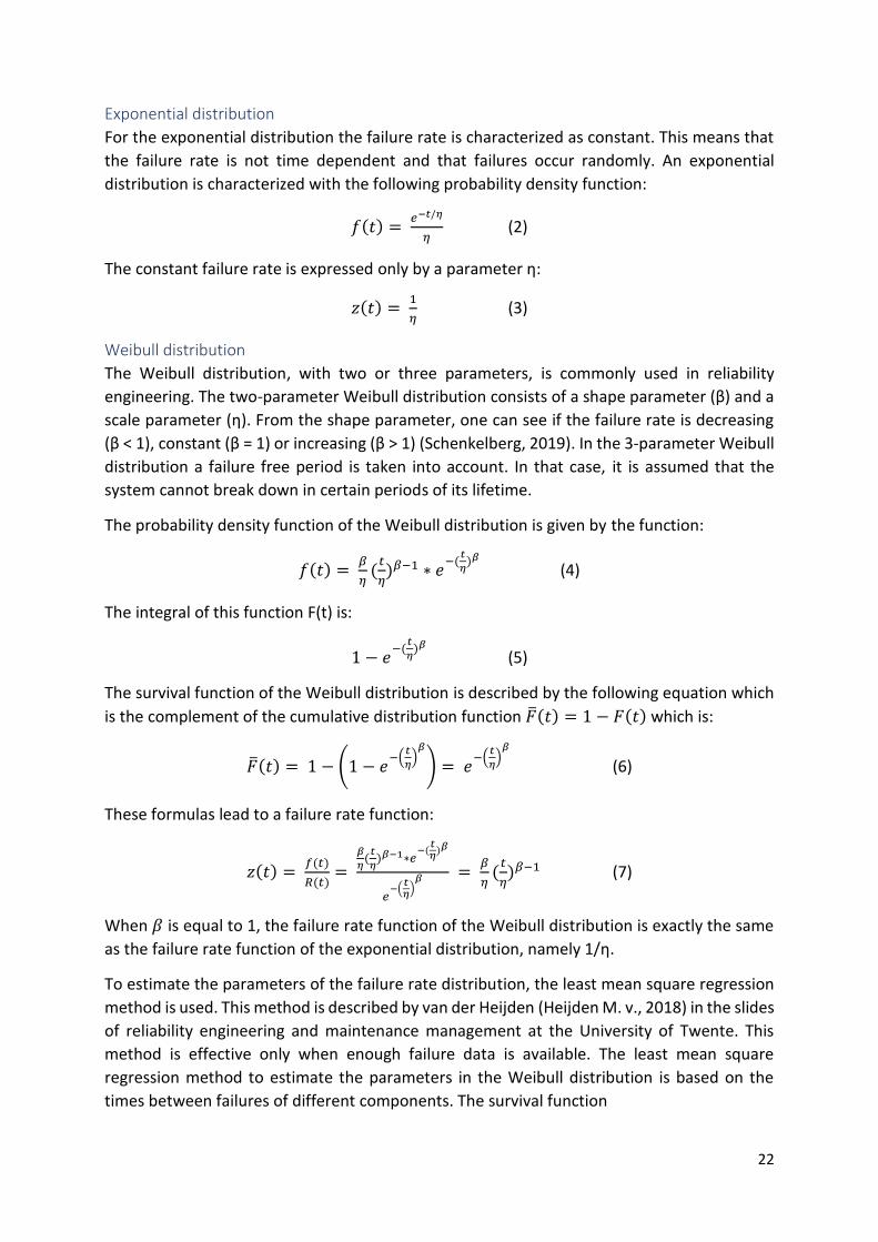
Exponential distribution

For the exponential distribution the failure rate is characterized as constant. This means that

the failure rate is not time dependent and that failures occur randomly. An exponential

distribution is characterized with the following probability density function:

𝑓(𝑡) = 𝑒−𝑡/𝜂

𝜂 (2)

The constant failure rate is expressed only by a parameter η:

𝑧(𝑡) = 1

𝜂 (3)

Weibull distribution

The Weibull distribution, with two or three parameters, is commonly used in reliability

engineering. The two-parameter Weibull distribution consists of a shape parameter (β) and a

scale parameter (η). From the shape parameter, one can see if the failure rate is decreasing

(β < 1), constant (β = 1) or increasing (β > 1) (Schenkelberg, 2019). In the 3-parameter Weibull

distribution a failure free period is taken into account. In that case, it is assumed that the

system cannot break down in certain periods of its lifetime.

The probability density function of the Weibull distribution is given by the function:

𝑓(𝑡) = 𝛽

𝜂(

𝑡

𝜂)𝛽−1 ∗ 𝑒

−(𝑡

𝜂)𝛽

(4)

The integral of this function F(t) is:

1 − 𝑒−(

𝑡

𝜂)𝛽

(5)

The survival function of the Weibull distribution is described by the following equation which

is the complement of the cumulative distribution function �̅�(𝑡) = 1 − 𝐹(𝑡) which is:

�̅�(𝑡) = 1 − (1 − 𝑒−(

𝑡

𝜂)

𝛽

) = 𝑒−(

𝑡

𝜂)

𝛽

(6)

These formulas lead to a failure rate function:

𝑧(𝑡) = 𝑓(𝑡)

𝑅(𝑡)=

𝛽

𝜂(

𝑡

𝜂)𝛽−1∗𝑒

−(𝑡𝜂

)𝛽

𝑒−(

𝑡𝜂

)𝛽 =

𝛽

𝜂(

𝑡

𝜂)𝛽−1 (7)

When 𝛽 is equal to 1, the failure rate function of the Weibull distribution is exactly the same

as the failure rate function of the exponential distribution, namely 1/η.

To estimate the parameters of the failure rate distribution, the least mean square regression

method is used. This method is described by van der Heijden (Heijden M. v., 2018) in the slides

of reliability engineering and maintenance management at the University of Twente. This

method is effective only when enough failure data is available. The least mean square

regression method to estimate the parameters in the Weibull distribution is based on the

times between failures of different components. The survival function

23

�̅�(𝑡) = 𝑒−(

𝑡

𝜂)

𝛽

(8)

can be rewritten as:

𝐿𝑛 (𝐿𝑛 (1

𝐹(𝑡))) = 𝛽(ln(𝑡) − ln(𝜂)) (9)

By applying linear regression with the dependent variables y(t) on the left-hand side and ln(t)

equals x(t) on the right-hand side, we can find the slope and the intercept with the y-axis. The

slope of the regression line is parameter β and the intercept with the y-axis (C) can be used to

calculate η by the following formula:

𝜂 = 𝑒−𝐶/𝛽 (10)

The goodness of fit is quantified by the coefficient of determination (R2) (Kvalseth, 1985). In a

linear regression model, the value of R2 is always be between 0 and 1. If the value is 0, there

is no better fit than a line through the mean of all points. This means that Y cannot be

predicted by X. On the other hand, when the value of R2 is exactly 1, all data points lie on the

curve and knowing the value of X, gives the value of Y automatically (GraphPad Software,

1995). So, the closer the value of R2 to 1, the better the fit of the linear regression model.

The estimations for the parameter β are important for maintenance planning. The value of β

indicates the cost effectiveness of preventive maintenance with β equal to or smaller than 1

indicating that preventive maintenance is not cost effective, and with β larger than 1 pointing

to a situation that the asset wears out over time and it is cost effective to carry out preventive

maintenance. (Abernethy, 2004). This is only true for cases where the costs for corrective

maintenance are higher than the costs for preventive maintenance.

Chi square test

The Chi-square test of independence is one of the most useful statistical techniques for testing

hypotheses with nominal variables (McHugh, 2015). The Chi-square test is used to find

whether the observed value differ significantly from expected value (Statistics Solutions,

2019). The term goodness of fit is a measure how a theoretical distribution fits an empirical

distribution. The sample data is divided over a certain amount of intervals. The number of data

points from the data set that belong to one interval is compared to the theoretical expected

number of data points in the according interval.

The Chi-square test does not only provide information on significance but can also tell which

categories are accountable for the difference. Secondly the variables should be mutually

exclusive and independent from each other.

The null hypothesis for the Chi-square goodness of fit test assumes that there is no significant

difference between the observed and the expected value. The alternative hypothesis is that

there is a significant difference between the observed and expected value (Statistics Solutions,

2019). The Chi-square value is the sum of the squared difference of the expected and the

observed number per category:

𝜒2 = (𝑂−𝐸)2

𝐸 (11)

24

Where O is the observed number in one category and E is the expected number in the same

category.

This formula is applied to every category of the data set and the sum of these values is the

total value of the Chi-squares:

∑ 𝜒2 (12)

This value is compared to a table value in order to test the null hypothesis. In case the Chi-

square value is higher than the table value, the null-hypothesis is rejected, thus concluding

that there is a significant difference between the empirical distribution and the theoretical

distribution. However, when the Chi-square value is smaller than the table value, the

conclusion is that there is no significant difference between the empirical and the theoretical

distribution.

The selection of table values depends on the degrees of freedom and the level of significance.

The degrees of freedom are dependent on the number of rows and columns in the table. The

number of rows is equal to the number of categories. The number of columns is equal to the

number of distributions you are comparing (Statistics Solutions, 2019). To conclude, the

number of degrees of freedom is (# of rows - 1)(# of columns - 1). A typical value for the level

of significance is 0.05.

3.3 Opportunistic maintenance Most conventional maintenance strategies are purely corrective or time-scheduled (Thomas,

Levrat, & Iung, 2008). Thomas suggests to move from a more traditional maintenance towards

condition based maintenance where maintenance is only carried out when a certain level of

deterioration occurs (Thomas, Levrat, & Iung, 2008). Anticipation allows to carry out

maintenance not only in response to a failure but also for opportunistic reasons. The key for

opportunistic maintenance is to answer the following questions: When to carry out a

maintenance action? What components should benefit from a preventive maintenance

action? What components should benefit first? (Thomas, Levrat, & Iung, 2008).

Initially, opportunistic maintenance, was considered as an opportunity if preventive

maintenance can be combined with corrective maintenance in order to make the set-up costs

decrease. (Thomas, Levrat, & Iung, 2008). In later studies by Radner and Jorgenson,

opportunistic maintenance was considered to be to opportunity to replace non-monitored

components in combination with the monitored components (Radnar & Jorgensen, 1963).

The aim of these policies is to minimize for example set up costs or production losses. From

this we define an opportunity as a period during which maintenance can be carried out

without loss or negative impact on production.

3.4 Discrete event simulation In this section we will look into the literature of a very common simulation study approach,

namely discrete event simulation.

Discrete event simulation is used for modelling queuing systems. Entities flow between

activities that are separated by queues. These queues appear when entities flow into the

25

queue faster with a higher rate than they flow out of the queue (Robinson, Simulation the

Practice of Model Development and Use, 2014).

Advantage of a simulation study over real-life experiments

Stewart Robinson describes the advantages of a simulation study over experimenting in a real

system. Although some points that are raised by Robinson seem straightforward, it is good to

emphasize the main advantages of a simulation study: (Robinson, Simulation the Practice of

Model Development and Use, 2014).

Costs. It can be costly to set up experiments in a real system. This would interrupt day-to-day

activities if one wants to try new things.

Time. It will be very time-consuming to change the experimental factors in a real system.

Besides, it will take a lot of time until the effects of the experimental factors will be reflected

in the real system. The results of a simulation study can be obtained in a timespan of minutes

to hours.

Control of the experimental conditions. In a real system, it is hard to compare experiments.

The most obvious reason is that some real life situations only occur once, so an experiment

can only be executed once. But there are also other factors that cannot be controlled in real

systems, which makes it hard to look at the effect of other parameters.

The real system does not exist. If the real system does not exist yet, it is better to build a

simulation model first to conduct experiments on beforehand, instead of building a series of

alternative real systems.

Fostering creativity. In a simulation study, out of the box ideas can be tested and improved in

an environment that is free of risk.

Advantages of a simulation study over other modelling approaches

Besides the advantages of a simulation study over real system experiments, Robinson points

out two advantages of simulation studies over other modelling approaches (Robinson,

Simulation the Practice of Model Development and Use, 2014).

Variability. The main advantage of a simulation study is that it is capable of perfectly modelling

variability in a system. If a system is subject to a significant level of variability, a simulation

study makes it possible to predict the performance of a system and the influence of the

experimental factors. Robinson illustrates this with an example of failing machines which are

analytically taken into account by averaging the failures with the process times, but can be

modelled much more detailed with a simulation study (Robinson, Simulation the Practice of

Model Development and Use, 2014).

Transparency. In order to show the results to a manager, a set of mathematical equations in

a spreadsheet might not be easy to understand or believe the results. A simulation study is

appealing since it is more intuitive to understand.

Disadvantages of a simulation study

Stewart Robinson also describes some disadvantages of a simulation study, which are good to

mention to give the simulation study a broader context.

26

Expensive. Simulation software is usually expensive and the price can even get higher when

external consultants have to be hired to develop the simulation model.

Data hungry. In order to create a simulation model that is a good representation of the real

system, a lot of data is needed. It might be the case that the data is not directly available and

must be processed first.

Requires expertise. Conducting a simulation study demands more than just programming

skills. The modeller should also have skills in conceptual modelling, statistics and validation.

This expertise is not always available at the company.

Over confidence. There is a danger that all the results that a simulation study shows are

considered to be right. When interpreting the results of a model, one should take into account

underlying simplifications and assumptions.

3.5 Conceptual model Before we start building a simulation model, we must design a conceptual model. The

conceptual model is defined as a non-software-specific description of the computer

simulation model that includes the objectives, inputs, outputs, content, assumption and

simplifications of the model (Robinson, Brooks, Kotiadis, & Zee, 2010).

- Following this definition, we will make a conceptual model that describes the

simulated model of the maintenance strategy for underground bins at Twente Milieu.

The main reasons for making a conceptual model according to Robinson et al are

(Robinson, Brooks, Kotiadis, & Zee, 2010) are i) to minimize incompleteness; ii) to

warrant the credibility of the model, iii) to provide a basis for the validation and

verification of the model; and iv) act as independent verification if that is required.

In his book “Simulation, the practice of model development” Stewart Robinson gives a

framework for the development of the conceptual model (Robinson, Simulation the Practice

of Model Development and Use, 2014). This framework consists of the following five key

activities: i) understanding the problem, ii) determining the modelling and project objectives,

iii) identifying the model outputs, iv) identifying the model inputs, and v) determining the

content (scope, assumptions and simplifications).

3.6 Experimentation Reliable experiments require an adequate the set-up. This section explains two important

factors of a simulation study, namely the warm-up period and the number of replications.

Warm-up period

A simulation model defines experiments for which input values can be altered. The result of

every simulation will give the KPI’s related to the input values of that experiment. In this way,

the influence of different input variables parameters on the costs for the maintenance

strategy is assessed. For carrying out the experiments, a warm-up period and a run length for

the simulation study are required.

The warm-up period is a way to deal with the initialization bias of a simulation model

(Robinson, Simulation the Practice of Model Development and Use, 2014). The warm-up

27

period should be long enough to ensure that the model is in a realistic condition before

extracting results and drawing conclusions. The bias comes from the fact that the simulation

model starts with an empty system with commonly unrealistic conditions. According to

Robinson, there are two main ways to determine the warm-up period, namely the graphical

method and the marginal standard error rule (MSER).

Robinson describes the MSER method to determine the warm-up period for experiments. The

aim of the MSER is to minimize the width of the confidence interval of the mean of the

simulation output after the initial transient data (Robinson, Simulation the Practice of Model

Development and Use, 2014).

The MSER method uses the following formula to determine the number of days after which

the warm-up period ends:

𝑀𝑆𝐸𝑅(𝑑) = 1

(𝑚−𝑑)2∑ (𝑌𝑖 − �̅�(𝑚, 𝑑))

2𝑚𝑖=𝑑+1 (13)

Where d is the proposed warm-up period, m is the number of observations in the simulation

output data and �̅�(𝑚, 𝑑) is the mean of the observations from 𝑌𝑑+1 to 𝑌𝑚.

Number of replications

To perform a proper simulation study, we also need to determine the number of replications

per experiment. If we carry out multiple replications for the same experiment, the stream of

random numbers changes per experiment, resulting in a better estimate of the mean

performance (Robinson, Simulation the Practice of Model Development and Use, 2014).

Robinson states that a rule of thumb by Law and McComas asks for three to five replications

per experiment. Robinson additionally explains a technique to determine the number of

replications by using the confidence interval of the mean value per experiment (Robinson,

Simulation the Practice of Model Development and Use, 2014). The idea behind this method

is that the narrower the confidence interval, the more precise the estimate of the mean value

is.

The technique starts by carrying out a lot of replications of one experiment and choose one

KPI to analyse. We take the mean value of this KPI for every replication. Then we compute a

cumulative mean and standard deviation over the performed replications. With these values

we can compute a confidence interval which narrows with every replication that is added. The

formula for the confidence interval is:

𝐶𝐼 = �̅� ± 𝑡𝑛−1,∝/2𝑆

√𝑛 (14)

Where �̅� is the mean of the replications, n is the number of replications, is the confidence

level and S is the standard deviation of the output of the replications. The level of significance

is set to 95%. The deviation of the confidence interval is how wide one half of the confidence

interval is compared of the value of the mean. We want the deviation to be lower than 2.5%

before we take the corresponding number of replications.

28

3.7 Relevance to this research Several ideas from literature described in this chapter are applicable to our research for

Twente Milieu. Distinction is made between preventive, corrective and opportunistic

maintenance. Especially for underground bins where customers notice directly when the bin

does not function properly and stay behind with their garbage, it is important to guarantee a

certain uptime for the underground bins. Preventive maintenance (Section 3.1.1) improves

uptime.

In order to carry out preventive maintenance, a certain preventive maintenance interval must

be chosen. Especially intervals based on usage-severity or on fixed time periods look

promising. Usage-severity based maintenance would take into account the usage of the bins

by customers, before it undergoes a preventive maintenance treatment of washing and

lubrication. In addition, time-based maintenance is investigated because of requirements set

by the municipalities and Twente Milieu themselves.

The modelling of a maintenance policy (Section 3.2) requires statistical techniques to

determine failure rate distributions and to compare empirical distributions with theoretical

distributions. The relationship between time to failure, survival rate and failure rate is

quantified. The Weibull distribution and the exponential distribution are commonly used

distributions for maintenance management. Then we elaborated on the theoretical

parameters for these distributions and identified linear regression as an adequate method to

determine the parameters of empirical distributions.

Another important maintenance strategy is opportunistic maintenance (Section 3.3). Because

the first and second line maintenance teams of Twente Milieu drive around the streets to carry

out corrective repairs, it might gain efficiency if underground bins that need corrective repair

are brought to Startpunt for preventive maintenance instead and be repaired correctively at

Startpunt at the same time. In the section 4.1 this will be referred to as corrective

replacement. The findings on opportunistic maintenance, worked out by Thomas et al

(Thomas, Levrat, & Iung, 2008), are used to develop such a strategy for Twente Milieu.

Section 3.4 elaborated on discrete event simulation, a main ingredient for empirical modelling. The theory behind simulation studies and the advantages and disadvantages of different simulation studies lead to the conclusion that discrete event simulation can be used to catch the variability that an analytical model cannot catch. Before starting a simulation study, a conceptual model (section 3.5) needs to be created to define the objective, input, output, scope and simplifications of the simulation study.

29

4. Modelling approach Chapter 4 describes the models that are used to analyse maintenance methods for the

underground bins. Section 4.1 describes maintenance methods that are carried out at Twente

Milieu. Section 4.2 describes the research outline of the next sections. Section 4.3 describes the

way to find an optimal preventive maintenance interval by using a cost function. Section 4.4

elaborates on optimizing a maintenance policy by carrying out a discrete event simulation

study. Section 4.5 describes the conclusions that we draw from chapter 4.

4.1 Maintenance methods The next part of this research considers four types of maintenance: corrective repair on the

bin site or at Startpunt (corrective replacement), and preventive maintenance for age-based

reasons or for opportunistic reasons:

Corrective repair on the bin site: This maintenance method is currently applied. After a

notification of a failed bin, the second line mechanics drive to the bin site and repair the bin.

Corrective replacement with repair at Startpunt: This maintenance method is added to the

desired situation. Failing bins on the street are replaced by an available bin from the stock at

Startpunt, the latter bins are as good as new. The failing bin is transported to Startpunt where

it is repaired and given a treatment of washing, lubrication and inspection. After this

maintenance treatment, the bin is as good as new and stocked at Startpunt.

Age-based preventive maintenance: This preventive maintenance method uses a preventive

maintenance interval that is based on findings in literature. An active bin is replaced after a

certain period called the preventive maintenance interval with an as good as new bin from

Startpunt. The bin from the street is transported to Startpunt to get washed, lubricated and

inspected.

Opportunistic preventive maintenance: Opportunistic maintenance as described in the

literature section 3.3 is intended increase the performance of the maintenance strategy. The

idea is to use the failure of a bin as an opportunity to carry out preventive maintenance to

another active bin in the same neighbourhood. This maintenance method comes with a

certain threshold to prevent that the time interval between two preventive maintenance

instances does not become too small.

30

Figure 11 shows a tree diagram of how the maintenance methods relate to each other.

Figure 11 Types of maintenance

These four maintenance methods come with different costs since the nature of the repair

differs.

Costs for downtime: Both corrective repair on the bin site and corrective replacement account

for downtime, so the costs for downtime must be taken into account for each maintenance

method in response to the failure of a bin.

Fees of the mechanics: The corrective repair at the bin site is carried out by the second line

mechanics who have a higher hourly fee than the Startpunt mechanics, who carry out the

other three maintenance methods at Startpunt.

Transportation costs: The three maintenance methods with preventive maintenance or repair

at Startpunt come with transportation costs from the bin site to Startpunt. The transportation

costs for the second line mechanics from bin to bin are included in the hourly fee.

4.2 Research outline The effects of the four types of maintenance we defined in the previous section must be

examined in order to determine an effective preventive maintenance strategy for Twente

Milieu. We start by analysing the cost function in formula 1 which we found in literature. This

cost function leads to an optimal preventive maintenance interval. The cost function

incorporates only two out of four maintenance methods from figure 11. Namely (i) corrective

repair at the bin site and (ii) age based preventive maintenance.

After analysing the cost function, we can incorporate the other two maintenance methods

from figure 11 (i) corrective replacement and (ii) opportunistic preventive maintenance in a

discrete event simulation model. This model analyses the performance of the maintenance

methods in terms of costs, downtime of underground bins and number of corrective repairs

31

by second line mechanics. Due to the ability of a simulation model to make decisions based

on events, we expect to improve the performance of the maintenance planning model.

In order to see how reliable the results are, we end the numerical analysis with a sensitivity

analysis. After the two numerical analyses, we can draw conclusions about the effectiveness

of maintenance policies and if Twente Milieu should implement the proposed policies.

4.3 Age-based maintenance In maintenance engineering, the optimal preventive maintenance interval for an underground

bin can be determined analytically by using the cost function G(t) based on the failure

distribution as described in section 3.1.1 (formula 1). The optimal interval is dependent on the

failure distribution, the costs of corrective maintenance and the costs of preventive

maintenance. The maintenance methods that are included in this study are (i) corrective

repair on the bin site and (ii) preventive maintenance at Startpunt. The costs of random

breakdowns leading to unforeseen downtime are important because of lost revenue and

customer dissatisfaction and can be included in the corrective maintenance costs.

The cost function G(T) defines the cost per period of time, given a certain preventive

maintenance interval. The cost function from chapter 3.1.1 (formula 1) is:

𝑔(𝑇) =𝐶𝑐 ∗ 𝐹(𝑇) + (1 − 𝐹(𝑇)) ∗ 𝐶𝑝

∫ (1 − 𝐹(𝑡))𝑑𝑡𝑇

0

F(t) is the cumulative distribution function for lifetime T. The numerator concerns the

expected costs per cycle and the denominator contains the expected cycle length. The

expected values are dependent on the lifetime distribution determined by the mean time to

failure (MTTF) of the underground bins.

To determine the optimal preventive maintenance interval analytically, we evaluate the cost

function g(T) for every T in days. Typically these kind of figures will present a given T for which

the costs per unit of time are the lowest.

Before computing such a graph, the failure distribution needs to be determined. Section 5.1

elaborates on the processing of the failure data to find a failure rate distribution F(t).

4.4 Discrete event simulation The age based maintenance model compares the effectiveness of two of the four described

maintenance methods, corrective repair at the bin site and preventive maintenance of

washing, lubrication and inspection at Startpunt. The other two described maintenance

methods, corrective replacement and opportunistic maintenance policies, can also add

effectiveness to the maintenance strategy but are not taken into account in the maintenance

planning model with the cost function. The cost function model does not include all variability

needed for this research and the maintenance methods opportunistic maintenance and

32

corrective replacement require more variability and decisions based on events than the cost

function model can give.

Another shortcoming of the cost function model is that it does not include the capacity of

Startpunt. The cost function results in a strict preventive maintenance interval minimizing the

maintenance costs per day. Such a strict maintenance interval implies that all bins should be

replaced by a new bin at the same moment, which is not feasible.

For the latter reasons, the simulation study incorporates the four described maintenance

methods, takes into account capacity issues and adds more variability to the model.

4.4.1 Opportunistic maintenance in the simulation model

Section 2.3 showed that most of the underground bins are inspected at least once a year. This

would imply that opportunistic maintenance policies as described in section 3.4 gain efficiency

in the maintenance process. In section 3.4 we described an opportunity as a repair of one

component that creates an opportunity to carry out preventive maintenance on other

components. Using this opportunity would combine two types of maintenance thus decrease

the set up costs. Opportunistic maintenance in this study requires a different analysis because

we do not consider different components of one underground bin. However, we will still call

it opportunistic maintenance since a failure of an underground bin gives the opportunity to

carry out preventive maintenance at Startpunt.

The idea is the following: Twente Milieu seeks to give a preventive maintenance treatment to

all underground bins with a regular interval. Such a regular interval depends on the planning

of using the available capacity at Startpunt. On beforehand, specific active underground bins

are selected to be replaced by fully repaired underground bins. The number of bins depends

on the specified interval and the available capacity at Startpunt. In case other non-functioning

bins need to be repaired Twente Milieu needs to deviate from the initial maintenance planning

and leave one of the pre-selected non-failing underground bins active and replace the one

that has just failed instead. Consequently, the second line mechanics do not have to go to the

failed underground bin for corrective repair, since the bin will be repaired in combination with

the rest of the washing, lubrication and inspection treatment at Startpunt. In the long run, this

should save time and labour for the second line mechanics.

4.4.2 Conceptual model

The five key activities for conceptual modelling as described in section 3.6.2 will be discussed

and elaborated on in the following sections. The five key activities are (i) understanding the

problem, (ii) setting the objective, (iii) choosing inputs, (iv) selecting outputs, and (v) setting

the scope.

Understanding the problem

The main problem description has been given in section 2.4 to 2.6 where the desired situation

by Twente Milieu concerning washing, lubrication and inspection is explained. Twente Milieu

seeks to optimize the maintenance of underground bins by combining maintenance on site (in

the streets) and at the workshops. The envisaged planning should combine the time-based

preventive maintenance with corrective maintenance at the workshops. A key issue

insufficient capacity at Startpunt to carry out preventive maintenance for all underground bins

33

at the same time. Besides this, the analytical model as described in section 4.1 and 4.2 does

not catch all variability that a discrete event simulation study can include. Variability is

important because of the model simulation of it and the subsequent simulation of the decision

taken based on variable actions in the model. For example, the simulation model allows

making decisions after a failure occurs. These decisions are possibly based on many factors

such as the last maintenance instance and the available stock of bins. Such a decision cannot

fully be analysed by a time-based preventive maintenance model.

Objective

According to Robinson (date), it is vital that the objectives of the model are known before

making a conceptual model, because without clear objectives it is not possible to create a

simplification of reality. In this case, the objective of the simulation model is to design a

method to give all underground bins the necessary maintenance treatments, corrective when

they break down and preventive when with a certain maintenance interval by minimizing the

costs. In addition to this objective, the workload at Startpunt needs to be evenly spread over

the available capacity thus minimizing the total maintenance costs for the full maintenance

method.

This objective is measurable and data on selected KPI’s in the simulation model are available.

This objective is achievable with the simulation model in this study that incorporates different

variables and the relationship between these variables.

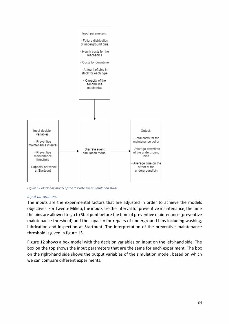
34

Figure 12 Black box model of the discrete event simulation study

Input parameters

The inputs are the experimental factors that are adjusted in order to achieve the models

objectives. For Twente Milieu, the inputs are the interval for preventive maintenance, the time

the bins are allowed to go to Startpunt before the time of preventive maintenance (preventive

maintenance threshold) and the capacity for repairs of underground bins including washing,

lubrication and inspection at Startpunt. The interpretation of the preventive maintenance

threshold is given in figure 13.

Figure 12 shows a box model with the decision variables on input on the left-hand side. The

box on the top shows the input parameters that are the same for each experiment. The box

on the right-hand side shows the output variables of the simulation model, based on which

we can compare different experiments.

35

In section 2.4 we explained that the capacity of Startpunt is limited, so the model uses a

minimum time a bin has to be on the street before it can go back to Startpunt at a failure. For

this, the variable ‘preventive maintenance threshold’ is introduced. This variable indicates the

time a failing bin is allowed to go to Startpunt for maintenance actions before regular

replacement time is reached. This has influence on the opportunistic maintenance strategy

since this strategy takes into account failures that occur before the moment of scheduled

preventive maintenance. In figure 13 the period after the preventive maintenance threshold

is indicated at the left-hand side.

Figure 13 explanation of threshold for preventive maintenance

Besides the experimental factors, the settings that are kept constant in experiments are also

part of the simulation model input. These settings include the number of bins on the street

and the failure rate distribution of these bins. The failure rate distribution is the same as used

in the analytical model (Section 4.2.). Since not all failures are mechanical failures there should

be a distribution that decides if the failure is mechanical and can be resolved at Startpunt.

Since all bins periodically need preventive maintenance, the simulation model should follow

a planning to process all bins at the right time. But this production scheme is not rigid. During

the simulation study, events can take place that change the production scheme for preventive

maintenance. To take these events into account, the conceptual process model depicts the

events and actions taken based on an event. An example of such an adaptive production

planning is that a failure of an underground bin can result in either a maintenance treatment

at Startpunt or on the bin site. If the broken bin is repaired at Startpunt, the bin gets an

additional treatment of washing, lubrication and inspection which is preventive maintenance.

The decision to transport the broken bins to Startpunt changes the schedule.

The decisions included in the simulation are shown in the flowcharts in appendix A and B. The

decision process starts when a bin fails (Appendix A). The decision on second-line mechanics

or repair at Startpunt is made by the maintenance engineer. A flow chart of the decision by

the maintenance engineer is shown in appendix B.

36

Outputs

The output of the model is defined by Robinson (Robinson, Brooks, Kotiadis, & Zee, 2010) as

the statistics that tell us if the objective has been reached. If the objective has not been

reached, the output should also show why the objective has not been reached. The main

output for this study’s model is the costs per year for the entire maintenance plan carried out

by Twente Milieu.

The costs of the output include:

- the costs for all maintenance actions both preventive and corrective,

- the costs for each day that a bin is unavailable,

- the purchase costs for each bin in the system,

- the costs for hiring the truck to transport underground bins from the street to

Startpunt.

The actual costs for maintenance actions are different from the analytical model in a few ways.

Firstly, a broken bin that is repaired at Startpunt for the costs of preventive maintenance has

been broken on the street as well, so the costs for downtime have been added to the repair

at Startpunt. These costs for downtime have been determined to €100,- for every day a bin is

unavailable. Since this is a rough estimation, we will test the sensitivity of the maintenance

strategy to the costs for downtime.

The transportation costs, which were a rough estimation in the maintenance planning model

as well, can be better specified based on available exact data on how many bins are

transported to Startpunt with driving costs of €1000,- a day.

The workload at Startpunt is also a model output that is important for Twente Milieu. The

model output should give the number of bins that is processed at Startpunt per week. The

capacity at Startpunt is one of the main reasons the simulation model is built, since not all bins

can get preventive maintenance at the same time.

The number of maintenance actions by the second line mechanics is also a model output. The

number of corrective repairs on bin site that they perform is also important. We expect that

number to decrease since more maintenance activities are taken over by the mechanics at

Startpunt who perform the washing, lubrication and inspection treatment together with the

repair of a broken bin if that happens.

The average amount of days that a bin is unavailable is also a measurable KPI in the simulation

model.

Lastly we determine the average time on the street of an underground bin and the standard

deviation of this average. This measure indicates whether bins are given preventive

maintenance frequently enough (on average).

Scope

The scope defines the possibilities and limitations of the simulation model.

The scope of the simulation is the combination of second line repair jobs and preventive

maintenance jobs carried out at Startpunt. We decided to leave out the corrective

37

maintenance jobs by first line mechanics since these jobs differ too much from the

maintenance jobs that can be done by mechanics at Startpunt.

The decision to leave out the first line is also due to the computed failure rate which was

exponential distributed. According to the literature (Heijden M. v., 2018) a beta value of

approximately 1 does not support a preventive maintenance strategy.

4.4.3 Assumptions, simplifications and verification

To make a modelled representation of the reality, assumptions and simplifications are

necessary. This section explains which assumptions were made in this simulation study.

Driving time between bins on the street is not taken into account: In the real life situation it is

useful to transport bins from the street to Startpunt which are close to each other. However,

if we only consider the municipality Hengelo, there are a lot of underground bins which are

relatively close to each other. In addition, the mechanics of Twente Milieu use route

optimizing software. The shortest routes between the bins cannot be included in the

simulation model because of programming limitation. Driving time is included in the capacity

of bin transportation on one day.

All underground bins have the same failure rate distribution: This assumption is justified by

the fact that all underground bins have the same mechanical structure. The only possible

difference is that the bins for residual waste have electronics inside to register cards from

customers. The failures concerning the electronics are resolved by the first line mechanics and

are beyond the scope of our research.

After corrective repair and preventive maintenance the failure rate starts again: In the

simulation model we assume that a broken bins are adequately repaired and mechanics also

verify the state of other components of the underground bin.

The exact process times at Startpunt are not taken into account: The process times at Startpunt

for washing, lubrication and inspection are not taken into account in the simulation models.

This would require data on the repair time per failure mode. This data is not available because

these kind of repairs are not carried out at Startpunt yet. The main implication of the lack of

this data is that the stock of underground bins cannot depend on the lead times in Startpunt.

This issue is resolved by setting the capacity of Startpunt of as an input variable for the model.

Lastly, to verify the model we check if the model follows logic reasoning, and the debugging

tools by Siemens Plant Simulation are used. By means of this tool each bin that fails is being

traced. It is checked what happens when the method of repair is decided by the model, either

at Startpunt or by the second line mechanics. And a last check verifies whether the model

adds the right numbers to the KPI tables and information tables. From extensive debugging, it

follows that the model follows the intended logic.

38

4.5 Conclusions of the modelling approach Sections 4.1 to 4.4 describe a manner in which we can build models to analyse proposed

maintenance policies at Twente Milieu. Section 4.1 elaborated on four maintenance methods

that should be incorporated in the models. We concluded that these four methods are (i)

corrective repair at the bin site, (ii) corrective replacement of failing bins, (iii) age-based

preventive maintenance and (iv) opportunistic maintenance.

Section 4.3 describes how we can set up a maintenance planning model based on the cost

function (Formula 1). The advantage of using this method is that with little computation time

we can find an optimal preventive maintenance interval for underground bins. The drawbacks

are that there are only two out of four maintenance methods involved, corrective repair at

the bin site and preventive maintenance at Startpunt.

Section 4.4 shows the conceptual model for a discrete event simulation study to analyse the

proposed maintenance strategies. The main advantage of carrying out a simulation study is

the inclusion of extra variability, the opportunity to respond to events and incorporation the

four maintenance methods from section 4.1.

The next section elaborates on the numerical analysis of both the time-based preventive

maintenance model and the discrete event simulation study.

39

5. Numerical analysis Section 5 elaborates on the numerical analysis of the cost function model and the discrete

event simulation model. The goal in chapter 5 is to analyse several maintenance policies and

find a way to optimize maintenance. Section 5.1 shows the failure distribution based on failure

data. Section 5.2 describes the implementation of the failure distribution in the cost function

in order to find the optimal preventive maintenance interval. Section 5.3 shows how the

implementation of the same failure distribution in the discrete event simulation model. Section

5.4 validates the simulation model with the reality. Section 5.5 describes the sensitivity analysis

to test the robustness of the results. Section 5.6 summarizes the results from the numerical

analysis.

5.1 Failure data The failure rate distribution of underground bins is necessary to design an analytical model

and to find the optimal preventive maintenance interval as described in section 3.2.1. This

section describes the methodology to collect and process the data.

5.1.1 Method of data gathering

Twente Milieu stores data in an online ERP system Wincar (Twente Milieu, 2015).

Maintenance jobs performed on any vehicle, underground bin or other appliance are

registered in this system. As a result, a lot of data is available on the frequency of visits to the

bins by mechanics and for what reason.

The data provides insight in the failure distribution of underground bins. Some choices and

assumptions on data selection are necessary. In the current situation practically only

corrective repairs are carried out by Twente Milieu. The only policy on preventive

maintenance is the outsourced washing, which is not taken into account in this study. This

means that the data is based on the failures and therefore suitable for a failure distribution

analysis; there is no interference of preventive maintenance.

Because the maintenance plan in this study concerns the underground bins in Hengelo, the

corrective maintenance data are on this municipality. The data include the maintenance jobs

by the first line and second line mechanics. The data is available from end 2013 and is still

updated since corrective maintenance is continued. This study uses the data of 2016 – 2018

on the corrective maintenance activities by Twente Milieu. These last three years the number

of underground bins in Hengelo has increased. This means that the last three years provide

sufficient data points that adequately take into account the increased pressure on

underground bin of the last years. The data of 2019 will be used to validate the model

afterwards.

One assumption we have to make because of the data availability is that the time of

maintenance is the moment of failure. This is not the real-life scenario since there is some

elapsed between the moment the failure occurs and the moment Twente Milieu is notified.

There is also some elapsed time between Twente Milieu is notified and the moment of

maintenance, but there is only data available of the moment of maintenance. However, the

difference between failure and repair is a matter of a few hours to a few days. That is on a

40

negligible scale compared to a life time of months to years, which justifies this assumption for

the time of failures.

An additional assumption is that each underground bin has the same failure rate. This

assumption is justified by the fact that the system and components of the underground bins

are almost identical. This means that the failure data of all bins apply to the failure distribution

of a single bin. Consequently, it is possible to use the general failure distribution to define an

optimal preventive maintenance interval for a single bin.

The relevant data available from Wincar concerns: unique number of the underground bin,

date of maintenance and executing mechanic (first of second line). There are two relevant

failure types are distinguished. Firstly the failures where the first line mechanics are

summoned to execute corrective repairs, and secondly the failure where the second line

mechanics are summoned to execute the corrective repairs. The nature of both types of failure

differs, because the first line mechanics usually repair bins that fail because of getting stuck

or because of electrical trouble. Second line mechanics carry out repairs to mechanical failures

in the inside structure of the underground bin. Probably the first line failures have more of a

random nature (customer actions) and second line failures have a nature that is more time

dependant. Due to these differences in nature, both failure types likely have a different failure

distribution. Note also that the failures that are repaired by first line mechanics are also

failures that are more easily repaired on the bin site. The electronic parts and the input shaft

are easily reachable from outside the bin by opening the underground bin. The second line

failures are also repairable on the bin site, but require more work.

5.1.2 Life time distributions

The time between failures can be obtained by extracting all dates an underground bin has

been visited from the total table. Then by sorting them in ascending order and subtracting two

consecutive maintenance dates, we find the number of days between two maintenance

activities. Based on our assumption, this can be seen as a time to failure for an underground

bin. By doing this for all underground bins in Hengelo for the years 2016 to 2018, we have a

large data set to find a failure distribution.

This sequence of actions results in a list of times to failure for each of the two relevant failure

types (i) first line and (ii) second line. The times to failure of the underground bins are

presented in figure 14 and 15. The number of bins is based on the rule of thumb for histograms

where the number of bins is the square root of the sample size. Clearly the histograms for first

line failures follow the indicators of an exponential distribution.

41

Figure 14 Histogram of times to failure of first line failures

Figure 15 Histogram of times to failure of second line failures

However, the failure rate function for second line failures seems to be distributed according

to a Weibull distribution. As we described in section 3.3, is the Weibull distribution commonly

used in maintenance management. For this empirical distribution the parameters η and β, are

0

100

200

300

400

500

600

700

18

.41

73

.65

12

8.8

8

18

4.1

2

23

9.3

5

29

4.5

9

34

9.8

2

40

5.0

6

46

0.2

9

51

5.5

3

57

0.7

6

62

6.0

0

68

1.2

4

73

6.4

7

79

1.7

1

84

6.9

4

90

2.1

8

Fre

qu

en

tie

Verzamelbereik

First line time to failure

Frequentie

0

10

20

30

40

50

60

70

43

,8

87

,6

13

1,4

17

5,2

21

9

26

2,8

30

6,6

35

0,4

39

4,2

43

8

48

1,8

52

5,6

56

9,4

61

3,2

65

7

70

0,8

74

4,6

78

8,4

83

2,2

Me

er

Fre

qu

en

tie

Verzamelbereik

Second line time to failure

Frequentie

42

estimated in order to fit a Weibull distribution. We use the least mean square regression

method described in section 3.3

We start ordering the times to failure in non-decreasing order in such a way that X1 ≤ X2 … ≤

Xn. After that, we calculate the natural logarithm of each time to failure, which can be seen as

the x(t) of the linear function we want to find. Then we calculate1 − �̂�(𝑋𝑖), we use 𝑖−0.5

𝑛 as

proposed by van der Heijden (Heijden M. v., 2018).

The linear regression function provides a variable coefficient for the two datasets. The variable

coefficient of ln(t) gives the estimated value of beta. Based on the histograms in figure 14 and

15 it is expected that the beta value of the first line failure rate is close to one. If that is the

case, the Weibull distribution would approach the exponential distribution and this is in

accordance with the histograms. We expect the value of the beta of the second line failure to

be larger than 1 since there are indications in the histogram that the failures are Weibull

distributed.

Table 3 Parameters of failure rate distributions

Failure/parameter β C η R2

First line 0.997 -4.4276 84.95781 0.969

Second line 1.280 -6.85303 211.6387 0.995

Table 3 shows the results of the least mean square regression. The hypotheses about the beta

are confirmed by the analysis. This means that the failure rate of first line failures is

exponentially distributed and random. The second line failure distribution shows the

characteristics of a Weibull distribution with wear out property. The failure rate is higher than

1, so a preventive maintenance policy can be useful. The first check to quantify the goodness

of fit is given by the R2 value that is the outcome of the regression analysis. We show the

values of R2 in table 3 as well. Al values of R2 are very close to one, which is an indication the

X is a good predictor for Y. The empirical distributions should be tested to the theoretical

Weibull distribution with the parameters β = 1.28 and η = 211.64.

For this, the Chi-square test we compute the expected number of data points in on bin for the

theoretical distribution. The number of bins is determined by the rule of thumb that the

number of bins is the square root of the number of data points (√𝑛) which is √397 = 19.9

thus 19 bins. So, we want to see how much the empirical distribution differs from the

theoretical distribution. The number of bins is determined the measure is the difference

between the two bins squared divided by the expected number of data points in a bin. The

results are shown in the table in appendix C.

The degrees of freedom for this Chi-square test are calculated as: (19-1)*(2-1) = 18 and the

significance is 0.05 which means a probability of 1 - 0.05 = 0.95. The Chi-square table value

28.87 and thus the value of the Chi-square test (19.86) is lower than the table value. This

means that we can conclude that the empirical data does not differ from the theoretical

Weibull distribution (β = 1.28 and η = 211.64) with a level of significance of 0.05.

43

From the Chi-square test we conclude that the failure distribution for the second line failures

are Weibull distributed with a level of confidence of 95%. The value of confidence is high

enough to use the Weibull distribution in the numerical analysis that we will carry out in

section 5.2 and the discrete event simulation study in section 5.3.

5.1.3 Discussion on data analysis

The parameter estimations are according to our estimations. The fact that the first line failures

are exponentially distributed is expected because a large part of the failures for the first line

is due to garbage bags that get stuck in the underground bin. These failures are not time

dependant since they randomly happen, for example when someone drops a bag that is too

large. Many other first line repairs are due to vandalism or abuse of the underground bins,

which also randomly occur.

The repairs which are carried out by the second line are because of failures of parts that are

not reachable for customers, and therefore they are not subject to human actions and

consequently subject to elapsed time. From this perspective the Weibull distributed failure

rate with the wear out property since β > 1 was expectable. According to literature, this

indicates that preventive maintenance can be an effective policy. We study this in section 5.2,

where we add the costs for maintenance actions to the research.

5.2 Numerical analysis for time-based preventive maintenance This section shows calculations for the optimal preventive maintenance interval based on the

cost function as described in literature section 3.1 and based on the failure distribution

presented in in section 5.1. In section 5.2.1 we will define the costs for maintenance actions

at Twente Milieu to analyse the cost total cost function.

5.2.1 Costs for preventive and corrective maintenance

In the previous section, we described the failure distribution for underground bins. The failure

distribution for second line failures seems to be suitable for a preventive maintenance policy,

since the Weibull distribution has a beta value that is higher than 1, which is in accordance

with values in literature (Heijden M. v., 2018). According to van der Heijden, a second criterion

for a suitable time-based preventive maintenance policy is that preventive maintenance is

cheaper than corrective maintenance. The cost estimations should show if that is the case and

provides information on the influence of the costs on the optimal preventive maintenance

interval (Heijden M. v., 2018).

Only the second line failures follow a Weibull distribution, an optimal preventive maintenance

interval based on the second line failure rate is computed. These failures are time dependent,

unlike the first line failures, and thus suitable for a time based preventive maintenance policy.

The failure rate distribution in section 5.1 is used to compute the graph for expected

maintenance costs per period of time. Prior to the calculation of the costs per period of time,

the costs for both corrective and preventive maintenance need to be defined.

The estimation of the costs for maintenance are based on the data at Twente Milieu. The first

estimates are made for corrective maintenance. The internal price Twente Milieu uses is €72,-

per hour per mechanic. The second line mechanics are always working together, so their total

44

prices is €144,- per hour. For a working day, Twente Milieu calculates 8 hours. So, for second

line maintenance there are daily costs of 1152 per day. Mechanics can handle about 5.5 bins

per day. This means that the costs for a corrective maintenance action are estimated at

1152/5.5 ≈ €209,- The €72,- for the mechanics include the costs for the truck they are driving

in and all other overhead costs for employing mechanics.

For preventive maintenance variable costs per bin are estimated at €1000,- divided by the

number of bins transported on that day plus additional labour costs, which are much lower

than for the corrective maintenance because the mechanics are being educated and do drive

around. Consequently more bins per day are handled. We estimate the costs of the mechanics

at Startpunt on €50,- per bin.

The costs for materials have not been taken into account, since these are about the same for

all types of maintenance and are sometimes part of the labour costs. The total costs have been

calculated in the table 4.

Table 4 Maintenance costs for the current and proposed maintenance policy

Type of costs Current preventive maintenance policy

Proposed time-based preventive maintenance policy

Hiring Truck (€) 0 1000 per day

Hiring BWaste for Washing, lubrication and inspection (€) 45 per bin per time 0

Corrective maintenance on the bin location (€) 250 per bin 250 per bin

Preventive maintenance at Startpunt (€) 0 50 per bin

Costs for downtime (€) 100 per day 100 per day

With these costs we can evaluate the costs per unit of time. This is including the estimated

number of 20 bins per day, which adds €50,- per bin to the preventive maintenance costs.

Costs for downtime

Section 2.2.3 mentioned the negative consequences of downtime of the underground bins

shortly. Although there is lost revenue since people do not pay the €1,20 fee and leave the

waste around the bin, a larger loss is in customer experience. Besides, this mess gives negative

attention in traditional media and on social media. On the long run, this also encourages other

people to leave waste behind without paying. In 2017 the council of Enschede discussed

measures to decrease the number of illegally disposed garbage bags. Most of the proposed

measures are costly in terms of extra employees, extra IT-systems or surveillance cameras.

Because the exact costs for downtime are hard to estimate, we analyse the effect of different

cost configurations on the optimal maintenance interval (Figure 16).

Since we see variability in the costs for corrective maintenance (we do not know the exact

costs for downtime) and for preventive maintenance (the costs depend on the number of

transported bins on one day), we decided to show the impact of the variability on the optimal

preventive maintenance interval in the graph in figure 16.

45

Figure 16 cost function G(T)

Table 5 Optimal maintenance intervals and effectiveness for several cost configurations

Preventive costs in euros (€)

Corrective costs in euros (€) T* in days Effectiveness

100 500 240 1.030011079

100 750 165 1.078120782

150 750 240 1.030011079

200 1000 240 1.030011079

100 1000 120 1.123926072

According to the data set and the costs for preventive maintenance and corrective

maintenance, the optimal maintenance interval depends on the ratio between the corrective

and preventive maintenance costs. This is shown in table 5. The higher the costs of corrective

maintenance compared to the costs for preventive maintenance, the shorter the optimal

maintenance interval becomes (Figure 16). If the costs of corrective and preventive

maintenance are close to each other, a time-based maintenance strategy becomes less

effective.

5.2.2 Discussion on maintenance interval

Twente Milieu seeks to give each underground bin a preventive maintenance treatment once

a year. The results in table 5 show that that maintenance intervals that become longer (240

days) are less effective. This is due to the relatively low value of beta. The beta value of 1.28

is quite close to 1 which is points to an exponential distribution thus indicating that preventive

maintenance might not be very effective.

The uncertainties in the costs for corrective and preventive maintenance make it hard to

determine the optimal maintenance interval, however a good indication of the effectiveness

of a preventive maintenance interval is visible in figure 16.

0,00

1,00

2,00

3,00

4,00

5,00

6,00

7,00

8,00

9,00

10,001

29

57

85

11

31

41

16

91

97

22

52

53

28

13

09

33

73

65

39

34

21

44

94

77

50

55

33

56

15

89

61

76

45

67

37

01

72

97

57

78

58

13

84

18

69

89

79

25

95

39

81

10

09

Cost functions for different maintenance costs

75;250 100;500 100;750 150;750 200;1000 100;1000

46

For a strict preventive maintenance interval of a specified number of days, the capacity of

Twente Milieu is not sufficient to give all underground bins a preventive maintenance

treatment within a short time. This means that the preventive maintenance treatment for the

underground bins must be spread over a certain period of time, depending on the capacity of

transportation and processing of bins. In the research question in section 1.3 we stated that

the new preventive maintenance strategy should fit within the financial and working capacity

of Twente Milieu.

The last discussion point on the results of the cost function is that it incorporates only

preventive maintenance at Startpunt and corrective repairs on the bin site. As we mentioned

in section 4.1, there are two other potentially useful maintenance methods that are not taken

into account in this maintenance strategy. These methods are corrective replacement and

opportunistic maintenance.

Because of the latter reasons, the cost function G(t) is not the best way to determine the

interval for preventive maintenance. It is better to combine the costs for preventive

maintenance with different parameters such as the capacity of Twente Milieu and different

approaches to determine which bins gets preventive maintenance. Therefore a simulation

study as described in the literature review section 3.5 is carried out in the next section.

47

5.3 Numerical analysis for discrete event simulation This section analyses the results from the simulation model. We start by explaining the KPI’s

and the experimental design and then present the results of the current situation compared

to the simulation model and the improvements that can be achieved by insourcing preventive

maintenance. The dashboard of the simulation model is shown in figure 17.

Figure 17, Dashboard of the discrete event simulation model

5.3.1 KPI’s

Before we start the numerical analysis we need to have some indication of the performance

of the current situation. We acquire this scenario by modelling failures that are repaired on

the bin site by the second line mechanics only, as the situation is now. This gives a good

indication of the values of the relevant KPI’s in the current situation according to the

simulation model. We mentioned the KPI’s already shortly in the output paragraph in section

5.3: the total costs for the maintenance strategy; the average time a bin is on the street before

preventive maintenance at Startpunt; the number of corrective repairs by second line

mechanics; and the average downtime of a bin after a breakdown.

The average time on the street is a relevant KPI only if preventive maintenance is included.

This KPI, together with the standard deviation of the time on the street, indicates if Twente

Milieu is able to give every bin preventive maintenance within the proposed preventive

maintenance interval. This KPI gives a useful insight, since it might be necessary to visit a bin

location for maintenance as well, for example due to smelly air or failures in the fixed

mechanics of the pit.

We expect that the number of maintenance actions increases by applying a preventive

maintenance strategy because the underground bins are repaired before the end of their

lifetime. On the other hand, this decreases the costs for maintenance since the bins are

repaired before they fail and consequently do not lead to negative consequences of failure.

48

5.3.2 Warm-up period

In order to determine the warm-up period and avoid the initialization bias as described in

section 3.6.3, we use a KPI that depends on the emptiness of the system. We choose the

number of failing bins per day in the baseline scenario without preventive maintenance. This

KPI is subject to the initialization bias because all bins start with the same failure rate and the

second line mechanics are directly available to fix it. This is not a realistic situation.

We ran the simulation for 10 years, thus m = 3650. The graph in figure 18 displays the output.

In the graph it is not very well visible but on after 16 days of warm-up period, de MSER(d)

value is minimal. Therefore all information from day 0 to day 16 is excluded in the simulation

model. Because the simulation study is non-terminating, we can use any period of days larger

than 16 as a warm-up period. With most settings for preventive maintenance interval and the

threshold, there is preventive maintenance at Startpunt in the first 20-30 weeks of the first

year. In order to overcome this period and for modelling purposes the monitoring of the KPI’s

starts after year 1.

Figure 18 MSER output

The method of confidence intervals (described in section 3.6.3) is used to determine the

number of replications per experiment and this number should match the rule of thumb by

Law and McConas. The upper and lower bound of the confidence interval are set by formula

14, with the results presented in Table 6.

Table 6 Simulation output to determine number of replications

Replication value

maintenance costs (€)

Cumulative mean

Standard deviation

Lower bound

Upper Bound

Deviation (%)

0

0,005

0,01

0,015

0,02

11

37

27

34

09

54

56

81

81

79

53

10

89

12

25

13

61

14

97

16

33

17

69

19

05

20

41

21

77

23

13

24

49

25

85

27

21

28

57

29

93

31

29

32

65

34

01

35

37

MSER output

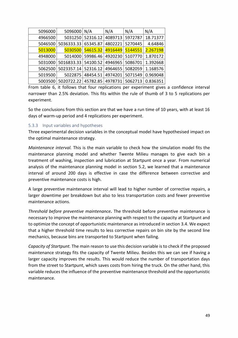
49

5096000 5096000 N/A N/A N/A N/A

4966500 5031250 52316.12 4089713 5972787 18.71377

5046500 5036333.33 65345.87 4802221 5270445 4.64846

5013000 5030500 54615.32 4916449 5144551 2.267198

4948000 5014000 59986.46 4920230 5107770 1.870172

5031000 5016833.33 54100.52 4946965 5086701 1.392668

5062500 5023357.14 52316.12 4964655 5082059 1.168576

5019500 5022875 48454.51 4974201 5071549 0.969048

5003500 5020722.22 45782.85 4978731 5062713 0.836351 From table 6, it follows that four replications per experiment gives a confidence interval

narrower than 2.5% deviation. This fits within the rule of thumb of 3 to 5 replications per

experiment.

So the conclusions from this section are that we have a run time of 10 years, with at least 16

days of warm-up period and 4 replications per experiment.

5.3.3 Input variables and hypotheses

Three experimental decision variables in the conceptual model have hypothesised impact on

the optimal maintenance strategy.

Maintenance interval. This is the main variable to check how the simulation model fits the

maintenance planning model and whether Twente Milieu manages to give each bin a

treatment of washing, inspection and lubrication at Startpunt once a year. From numerical

analysis of the maintenance planning model in section 5.2, we learned that a maintenance

interval of around 200 days is effective in case the difference between corrective and

preventive maintenance costs is high.

A large preventive maintenance interval will lead to higher number of corrective repairs, a

larger downtime per breakdown but also to less transportation costs and fewer preventive

maintenance actions.

Threshold before preventive maintenance. The threshold before preventive maintenance is

necessary to improve the maintenance planning with respect to the capacity at Startpunt and

to optimize the concept of opportunistic maintenance as introduced in section 3.4. We expect

that a higher threshold time results to less corrective repairs on bin site by the second line

mechanics, because bins are transported to Startpunt when failing.

Capacity of Startpunt. The main reason to use this decision variable is to check if the proposed

maintenance strategy fits the capacity of Twente Milieu. Besides this we can see if having a

larger capacity improves the results. This would reduce the number of transportation days

from the street to Startpunt, which saves costs from hiring the truck. On the other hand, this

variable reduces the influence of the preventive maintenance threshold and the opportunistic

maintenance.

50

5.3.4 Experimental design

The testing of three variables in a broad range in a full factorial experimentation would require

too much running time. A full factorial experimental design includes tests of all combinations

of input factors in order to see exactly which settings for the input variables gives the best

results. Next to that, the full factorial experimental design has to be carried out four times

because of required replications. For example, testing the capacity of Startpunt between 12

and 40, the preventive maintenance threshold from 20 days to 80 days with an increment of

10, and the maintenance interval between 300 and 400 days with and increment of 10 would

lead to 29*7*11 = 2233 experiments to be carried out in fourfold. With 10 seconds per run,

this would require a running time of 25 hours. This phenomenon is described as the problem

of combinations by Robinson (Robinson, Simulation the Practice of Model Development and

Use, 2014).

We need to define our experiments in such a way that the running time shortened to at most

3 hours, which means about 300 experiments at most.

Therefore we narrow down the range to 13 to 18 bins, a preventive maintenance interval

range from 260 to 360 days and just two values for the preventive maintenance threshold,

namely 60 and 90. From these experiments we find the influence of the three decision

variables on the costs, the average downtime and the number of maintenance activities.

Following this set of 132 experiments, we can search in smaller ranges of decision variables.

This leads to an adapted search with fewer experiments.

5.3.5 Results

This section compares the results of the modelling of the current situation without preventive

maintenance at Startpunt and the desired situation with insourced preventive maintenance.

The main reason to model the current situation instead of taking the costs that are made in

reality is that we can compare modelled situations. If we would take the costs that are made

in reality, the comparison with the outcomes of the simulation model would be less reliable.

Outsourced scenario

In the outsourced scenario generated failures are repaired by second line mechanics. This

gives an indication of the performance of the system in the current situation. In this scenario,

there is no preventive maintenance and thus the maintenance interval and the preventive

maintenance threshold do not matter as input variables.

The output includes the costs for the maintenance strategy, the average downtime after a

failure and the number of repairs are taken into account. The average time on the street is

not measured, because this is only a measure in the scenario where Twente Milieu carries out

the preventive maintenance actions.

51

For the current situation with outsourced preventive maintenance and corrective repair at the

bin site we have the input shown in table 7.

Table 7 Configurations of simulation model to analyse the current situation

Preventive maintenance False

Costs corrective maintenance

€400

Costs for a day down €100

Alpha 211.6

Beta 1.28

Warm-up 1 year

Run length 10 years

Number of bins 544

The maintenance costs include the costs for second line mechanics who repair each broken

bin on the bin site and the costs for downtime which is set to €100 per day. The costs of

purchase and amortization are added to compare scenarios with more bins available for

replacement of underground bins. Estimates by Twente Milieu employees result in a price of

2.750 Euro per bin and an amortization period of 15 years. The additional BWaste costs are

the costs for outsourcing washing, lubrication and inspection on the bin site, where BWaste

charges €85.00 per bin for two maintenance activities in a year). Table 8 provides the results

for the baseline scenario with outsourced preventive maintenance on the bin site and

corrective repair on the bin site by Twente Milieu mechanics.

Table 8 Results of the current situation analysis

KPI Simulation outcomes Per year

Maintenance costs (€) 4844875 €538319.44

Purchase and amortize costs (€)

544*2750= €1496000 1496000/15= €99733

Additional costs BWaste (€)

544*85= €46240

Downtime (days) 1.286

Total costs (€) 684293,-

Number of corrective maintenance actions

9161 1018

Preventive maintenance at Startpunt

For the simulation study on the effectiveness of preventive maintenance at Startpunt the

three input variables mentioned earlier are used: the preventive maintenance interval, the

preventive maintenance threshold, and the capacity of bins per week. The objective of the

modelling is to minimize the maintenance costs by modifying the input variables. The costs of

the preventive maintenance strategy should preferably be lower than the costs of the

outsourced scenario in the previous paragraph. Secondly we hope that the outcome of the

experiments lowers the average downtime of the underground bins.

52

In the first experimental design we carried out the experiments as shown in table 9 with a full

factorial design. This lead to a total of 11*2*6 = 132 experiments. This number is feasible

considering the amount of data generated and the running time. These can be seen as

exploratory experiments to investigate the influence of the three input variables.

Table 9 Ranges of experimental factors for simulation model

Variable Minimum Maximum Increment

Maintenance interval (days) 260 360 10

Threshold (days) 60 90 30

Capacity Startpunt (bins per week) 13 18 1

Figure 19 shows the influence of the preventive maintenance interval in days (x-axis) on the

annual maintenance costs. The annual costs decrease when the preventive maintenance

interval decreases. The main reason for the decreasing costs are the lower fees for the

mechanics at Startpunt and the decreased downtime. A short preventive maintenance interval

leads to a high pressure on Startpunt due to the ambition to carry out preventive maintenance

more often. The drawback of this policy is visible in the average time and the standard

deviation of the length of stay on the street before preventive maintenance.

Figure 19 Results of the second simulation run

Next, we look at the influence of the threshold time on the total costs for maintenance. A

higher threshold means that it is allowed to treat bins with corrective maintenance at

Startpunt shorter after a previous visit to Startpunt. The influence of a higher threshold is that

more failures are repaired at Startpunt, since it is allowed earlier, but this also means that

broken bins can stay on the street a few days longer because the transport for corrective

maintenance at Startpunt is not on a daily basis, in contrast to corrective repair at the bin site.

Hence, there is a trade-off between costs for downtime on the street and cheaper labour at

Startpunt.

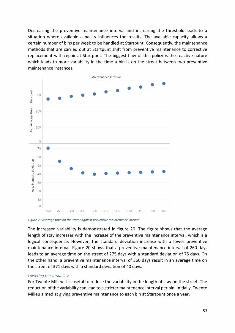
53

Decreasing the preventive maintenance interval and increasing the threshold leads to a

situation where available capacity influences the results. The available capacity allows a

certain number of bins per week to be handled at Startpunt. Consequently, the maintenance

methods that are carried out at Startpunt shift from preventive maintenance to corrective

replacement with repair at Startpunt. The biggest flaw of this policy is the reactive nature

which leads to more variability in the time a bin is on the street between two preventive

maintenance instances.

Figure 20 Average time on the street against preventive maintenance interval

The increased variability is demonstrated in figure 20. The figure shows that the average

length of stay increases with the increase of the preventive maintenance interval, which is a

logical consequence. However, the standard deviation increase with a lower preventive

maintenance interval. Figure 20 shows that a preventive maintenance interval of 260 days

leads to an average time on the street of 275 days with a standard deviation of 75 days. On

the other hand, a preventive maintenance interval of 360 days result in an average time on

the street of 371 days with a standard deviation of 40 days.

Lowering the variability

For Twente Milieu it is useful to reduce the variability in the length of stay on the street. The

reduction of the variability can lead to a stricter maintenance interval per bin. Initially, Twente

Milieu aimed at giving preventive maintenance to each bin at Startpunt once a year.

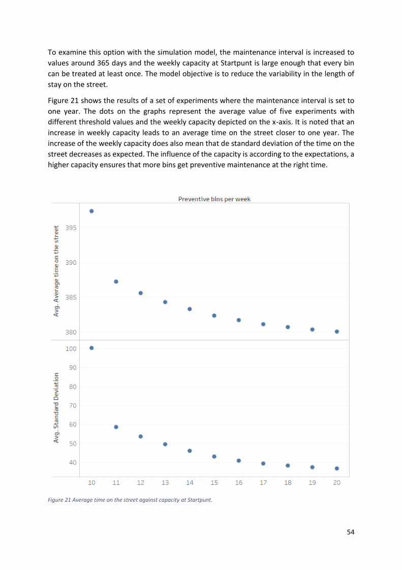
54

To examine this option with the simulation model, the maintenance interval is increased to

values around 365 days and the weekly capacity at Startpunt is large enough that every bin

can be treated at least once. The model objective is to reduce the variability in the length of

stay on the street.

Figure 21 shows the results of a set of experiments where the maintenance interval is set to

one year. The dots on the graphs represent the average value of five experiments with

different threshold values and the weekly capacity depicted on the x-axis. It is noted that an

increase in weekly capacity leads to an average time on the street closer to one year. The

increase of the weekly capacity does also mean that de standard deviation of the time on the

street decreases as expected. The influence of the capacity is according to the expectations, a

higher capacity ensures that more bins get preventive maintenance at the right time.

Figure 21 Average time on the street against capacity at Startpunt.

55

Hence, a higher threshold value and a higher capacity are beneficial to the average time on

the street and lower the standard deviation. Consequently, we can take a closer look to the

results of individual experiments.

To find a low enough standard deviation, we filter the results in appendix D in such a way that

we don’t show the weekly capacity of 10, due to the high standard deviation. Then we find

the lowest costs at the configurations shown in table 10.

Table 10 optimal configurations according to the objectives of Twente Milieu

Maintenance interval 365

Threshold 60

Capacity per week 19

Table 11 shows the values of the KPI’s corresponding to these settings. These values do fit the

objectives of Twente Milieu. Namely, the average time on the street before preventive

maintenance at Startpunt is just more than 365 days and the standard deviation of 37 days is

reasonably low.

Table 11 KPI's at the optimal configurations

KPI Simulation outcomes Per year

Maintenance costs (€) 4797443 533049

Purchase and amortize costs (€)

(544+33)*2750=1504250 1504250/15=100283

Additional costs BWaste (€)

Downtime (days) 1.07

Total costs (€) 633332

Number of corrective maintenance actions

8279 920

Average time on the street (days)

378.52

Standard deviation time on the street (days)

37.33

Table 12 compares the latter scenario and the current situation with outsourced preventive

maintenance. The scenario of using a preventive maintenance interval of one year shows

serious improvements on all three KPI’s.

Table 12 Comparison between optimal configurations and the scenario with outsourced preventive maintenance

KPI Outsourced scenario Averaging a year Improvement (%)

Yearly costs 684292.78 633332.31 7.45

Average downtime 1.29 1.07 16.75

Corrective maintenance per year 1017.86 920.00 9.61

56

Implementing a maintenance strategy that combines opportunistic maintenance at Startpunt

with corrective replacement, corrective repair at the bin location results in an improvement

compared to the scenario with outsourced preventive maintenance and only corrective repair

by second line mechanics. The improvements decrease the maintenance costs, decrease the

downtime due to failing bins and decrease the number of corrective repairs by second line

mechanics.

The proposed maintenance strategy creates work for Startpunt by giving preventive

maintenance to each bin in Hengelo on a yearly basis. The extra jobs match the social objective

of Twente Milieu to offer social employment combined with education. The saved time for

the second line mechanics by the implementation of corrective replacement can be used at

other places in the organization. Firstly, there are still seven other municipalities with failing

bins that need repair on a daily basis. A higher availability of the second line mechanics will

lead to a quicker repair and also a higher uptime of bins in these municipalities. Secondly, their

expert knowledge can be used at Startpunt to teach and support the Startpunt mechanics with

maintenance actions. The preventive maintenance is about the same for all bins at Startpunt,

but the repair of a failing bin requires some extra guidance.

5.4 Validation This section seeks to validate the results of the discrete event simulation with the real number

of failures from the failure data at Twente Milieu. We used the data of the first half of 2019 to

see how many failures that are resolved by second line mechanics actually occurred. In the

first half of 2019, the second line mechanics repaired 208 bins in Hengelo, this would mean

that the total number of failing bins per year lies around 400. The simulation model generates

1018 failures per year (table 8), which is a large overestimation compared to reality.

The influence of this overestimation does not make the results of the simulation study useless.

Firstly, the scenario with outsourced preventive maintenance uses the same failure

distribution as the new situation, which still shows that using the proposed maintenance

strategy leads to an improvement on all three KPI’s. Secondly, if it’s true that there are fewer

failures in real life, Twente Milieu can use a maintenance planning with even less variability or

an higher preventive maintenance interval and try to scale up to other municipalities quicker.

To see how the two models used fit together, we validate the results we found in the

simulation study with the results of the age-based maintenance policy. From these results, we

can conclude that both modelling techniques find an optimal preventive maintenance interval

between 160 and 200 days. This means that these models do correspond to each other and

justifies the step to extend this research with a discrete event simulation study.

5.5 Sensitivity analysis We see that the results of the simulation give better results than the maintenance planning

model of chapter four and that there are improvements in terms of costs, average downtime

and maintenance actions by second line mechanics by insourcing preventive maintenance.

However, with such a simulation study, we must be careful with the input parameters. In order

to see how robust this solution is and how the parameters such as the failure distribution and

input costs influence the outcomes of this simulation study.

57

First, we consider the failure distribution. From the data at Twente Milieu we found the

Weibull distribution with β 1.28 and η 211,6 this results in a mean time to failure of 195 days

according to the following formula:

𝐸(𝑇) = 𝜂 ∗ 𝛤(1 +1

𝛽) (15) (Heijden M. v., 2018).

This value might be a bit low, so we see what happens if we increase the value of eta. We

expect to have fewer failures thus increasing the preventive maintenance interval.

If the costs for corrective maintenance decrease, the strategy becomes less effective.

Similarly, if the costs for downtime decrease, the average downtime accounts for less added

costs so in that scenario, the proposed scenario might also lose improvement.

For the sensitivity analysis, we used the settings with the lowest costs, namely the preventive

maintenance time of 365 days, a weekly capacity of 19 bins and a preventive maintenance

threshold of 60 days.

With these decision variables settled, it is verified if insourcing preventive maintenance would

still be useful, although the costs and the failure rate are wrongly estimated.

In figure 22 we see that for all cost configurations the proposed maintenance strategy gains

improvement. However 1.26% for the lowest corrective maintenance costs and a downtime

cost of €50 per day is not too good. However, for all other cost configurations the

improvement percentages are still pretty good.

Figure 22 Results of the sensitivity analysis based on different cost parameters

Besides these percentages, it should be realized that the simulation model has not been used

to minimize the costs for the maintenance strategy in the sensitivity analysis, so if the cost

estimation seems to be too optimistic or too pessimistic, the same simulation model can be

used to find an optimal preventive maintenance interval again.

58

The next thing to check is how sensitive the proposed solution is considering the failure

distribution. As we mentioned earlier, we had the feeling that the number of failures is a bit

high, so we decided to change the value of eta from 211 days to 250, 300 and 350 days to see

the influence on the results of the proposed solution.

Table 13 shows the results for the different values of eta.

Table 13 Results of the sensitivity analysis based on different values for eta

Eta Outsourced costs per year

Insourced costs per year

Improvement

250 588528.89 559800.69 4.88%

300 509006.67 485838.89 4.55%

350 453203.89 437188.89 3.53%

So with the same settings but with a different value for eta, the KPI’s still improve. There is

still no optimized maintenance interval in the sensitivity analysis. If new or better failure

data becomes available, the simulation model can optimize the preventive maintenance

strategy by using the new failure data.

5.6 Conclusions of the numerical analysis Section 5.2 showed the results of the numerical analysis of the cost function. The cost function

of formula 1 is used in literature to find the optimal preventive maintenance interval given the

failure distribution and the costs for preventive and corrective maintenance. In this research,

the cost function method takes into account two out of four maintenance methods. These are

corrective repairs at the bin site and preventive maintenance at Startpunt. The analysis of the

cost function results in interesting insights on an effective maintenance interval. Firstly, that

a preventive maintenance strategy is effective given the input parameters of the Weibull

distribution and the costs for maintenance instances. Secondly, the optimal preventive

maintenance interval depends strongly on the ratio of costs for corrective maintenance and

preventive maintenance. These results are conforming to the literature findings in chapter 3.

However, implementing a strict preventive maintenance of 260 days directly is practically

infeasible for Twente Milieu and does not take into account all four described maintenance

policies. Namely (i) corrective repair, (ii) corrective replacement, (iii) age based preventive

maintenance and (iv) opportunistic preventive maintenance. Consequently, we extend our

research with a discrete event simulation study that gives more insights in the performance

of the four maintenance policies, in the decisions that can be made based on events and allows

us to introduce corrective replacement and opportunistic preventive maintenance.

The aim of the simulation study is to find a maintenance policy that reduces the maintenance

costs, reduces downtime of underground bins and reduces the number of maintenance

actions for second line engineers. We use the simulation model to determine the minimum

weekly capacity of Startpunt. The simulation model does also show more detailed results for

KPI’s such as downtime, number of corrective repairs and the average time on the street of

underground bins.

59

The results of the discrete event simulation look very promising. Firstly, implementing a

preventive maintenance threshold is the first step to deal with the capacity issues. Such a

preventive maintenance threshold is a minimum number of days that a bin should be on the

street before it is allowed to go to Startpunt for preventive maintenance. The threshold should

prevent that bins get preventive maintenance too often, but should ensure that not all bins

arrive at Startpunt at the same time due to a strict preventive maintenance interval. From the

results we can see that using a higher threshold results in lower costs for maintenance.

Secondly, a smaller preventive maintenance interval additionally leads to lower costs. Both

these effects are partly due to the difference in costs between preventive maintenance and

corrective maintenance. The results of the simulation study are quite sensitive to the ratio

between costs for preventive maintenance and corrective maintenance. The impact of the

costs is clearly shown in the sensitivity analysis. If the costs get closer to each other, gains in

terms of money of the maintenance strategy decrease. However, there are still gains visible

by looking at the downtime and the number of maintenance actions by second line mechanics.

In many configurations with low costs, the undesirable consequence of a high threshold and

a small preventive maintenance interval is the big variance in the average time on the street.

When the variance of the average time on the street is too high, a strict preventive

maintenance schedule cannot be followed, since bins visit Startpunt more irregularly.

In order to decrease the variance in the time on the street, we examined the options with a

preventive maintenance interval of one year as desired by Twente Milieu. The goal of the

experiments was to lower the variance and apply a more stringent maintenance interval per

bin, as initially desired. The main result of having a year as preventive maintenance interval

and having enough capacity is that the variance indeed decreases to values of 37 days, with

an average number of 370 days on the street.

60

6. Conclusions and recommendations In this chapter we will mention the most important conclusions of the research on insourcing

preventive maintenance at Twente Milieu. Section 6.2 addresses the steps Twente Milieu

should take to implement the proposed maintenance policy. Section 6.3 gives

recommendations for further research. To conclude, section 6.4 explains the contribution of

our research to literature and practice.

6.1 Conclusions This research at Twente Milieu aims to insource preventive maintenance treatment of

washing, inspection and lubrication of underground bins at Startpunt. In order to reach that

goal, we looked at the maintenance data of the first and second line mechanics. We concluded

in chapter 2 that many bins were already visited at least once a year, so these visits could be

used as opportunities to combine preventive maintenance and corrective maintenance.

From this starting point, we searched into literature to find information on optimizing

preventive maintenance, opportunistic maintenance strategies. According to literature, the

maintenance policies can be analysed numerically by using the cost function and discrete

event simulation.

We found information on how to find an optimal preventive maintenance interval given the

costs for preventive and corrective maintenance and a failure distribution. In chapter 4 we

conclude that the failures of underground bins are distributed according to a Weibull

distribution with a β value 1.28 and a η value 211.6. Secondly, it was hard to estimate the

costs for downtime and for corrective maintenance, since the downtime costs are part of the

corrective maintenance costs. Besides, it was also hard to estimate the transportation costs

which should be included in the preventive maintenance costs. We calculated the optimal

preventive maintenance interval and its effectiveness using the cost function G(T), for several

cost configurations to see the influence of costs. We conclude that a preventive maintenance

policy could be effective for Twente Milieu to lower the maintenance costs, but that

minimizing the cost function does not lead to big reductions of the maintenance costs. We can

conclude from the maintenance planning model with cost function G(T) (formula 1) that using

a preventive maintenance strategy for underground bins leads to slight improvements.

Therefore we decided to use a simulation model to seek for more improvements by using

different maintenance policies.

In order to introduce more of the real life variability in the maintenance optimization model

and to be able to include opportunistic maintenance as described in literature, we decided to

create a discrete event simulation model. By means of this simulation study, we concluded

that we can lower the costs for maintenance on underground bins in two ways.

61

We could take the preventive maintenance interval of 240 days that corresponds to the

preventive maintenance interval we found by using the cost function in combination with

using opportunistic maintenance for failing bins and introducing a preventive maintenance

threshold. This approach leads to a lot of corrective replacement since the policy allows bins

to be repaired at Startpunt shortly after they are installed on the street. This also means that

bins that do not fail stay on the street for a longer time then their preventive maintenance

interval due to the lack of capacity at Startpunt. This leads to a high variance in the average

time on the street. This variance is undesirable, since Twente Milieu aims to get every bin to

Startpunt at least once a year.

We could also increase the preventive maintenance interval to one year to reduce the

variance in the time a bin is on the street. These configurations still account for 7.6% cost

savings and 16.25% of downtime savings. Secondly setting a larger preventive maintenance

interval gives the options to see if an expansion to other municipalities such as Enschede or

Borne lies within the opportunities of Twente Milieu.

Both options account for improvements on the costs for the preventive maintenance strategy,

reduction of downtime of underground bins and reduction of the number of maintenance

actions by second line mechanics. Using a preventive maintenance interval of one year fits

better in the practical wishes of Twente Milieu and is less sensitive to overestimations of the

costs and the number of failures per year.

6.2 Recommendations for Implementation As demonstrated in the numerical analysis, insourcing preventive maintenance is an effective

strategy for Twente Milieu, to employ Startpunt mechanics and decrease the downtime. This

section describes the steps that should be taken to implement the proposed preventive

maintenance strategy.

Starting the proposed maintenance strategy has low set up costs, since the right materials are

present in the workshop of Startpunt and hiring a truck from BWaste can be done per day that

transport is needed. As long as there are repaired bin in stock, the truck can be used for one

day to replace a selection of active bins by bins from stock.

The bins that enter Startpunt get preventive maintenance of washing, lubrication, inspection

and necessary extra repairs. The first few weeks of implementation must be used to keep track

of the number of bins that Startpunt can handle in one week. When Startpunt is (almost) done

with handling the bins for one week, other bins must be transported from the street to

Startpunt. These bins can be chosen based on the location near a failing bin to reduce travel

time (opportunistic maintenance), based on a direct failure (corrective replacement) or based

on the current status of the bin obtained from the last round of inspection.

The last time a bin has had preventive maintenance must be stored in Wincar to keep track of

the time on the street and when the preventive maintenance interval of one year is

approaching.

62

This information can be used to design a schedule which determines the bins that should get

preventive maintenance at the next transportation day. Whenever a bin failure occurs, the

maintenance engineer can decide how to repair it. Due to the nature of the failure the second

line mechanics need to repair it on bin site, or corrective replacement can be used to repair

the broken bin at Startpunt. Reasons for corrective repair can be that the preventive

maintenance threshold has not been reached, or the failure cannot be repaired at Startpunt.

We advise to use the full weekly capacity of Startpunt in order to see what the opportunities

are to scale up the preventive maintenance area to Hengelo and Enschede, where mainly the

same type of underground bins are used. In the first year after implementation the data will

show if the quality of the maintenance improves and if the downtime of the underground bins

decreases.

6.3 Recommendations for further research In this section we will address some recommendations for further research.

Update the failure distribution: By treating bins more often at Startpunt, the failure

distribution might change. We have this expectations due to interviews with the maintenance

engineers. The quality of maintenance at Startpunt with an empty bin and all tools available

should be higher than a quick treatment on the street by BWaste. A while after

implementation, the change in failure distribution might be visible and could lead to the

necessity of a new maintenance policy with different preventive maintenance intervals.

Updating the failure distribution, can also lead to a better validated simulation model. This

would make the results of the research more reliable.

Add use-based maintenance: We expect that some bins are visited more often by second line

mechanics simply because they are used more often by customers because they are located

in more densely populated areas of the municipality. It could be interesting to analyse how

the usage influences the failure distribution. This could lead to different maintenance

strategies for different underground bins. Such an adapted maintenance policy might prevent

that bins that are used fewer times get unnecessary maintenance treatments which are costly

in terms of working hours and transportation.

Add lead times of the processes at Startpunt: When the processes of Startpunt have started,

it is possible to see in what state the bins are transported to Startpunt, what are the main

failure modes and how long it takes per failure mode to repair and wash, lubricate and inspect

every bin. This will give insight in the lead times for maintenance actions at Startpunt. These

lead times can be used to determine the necessary safety stock levels and the number of bins

that can be handled in one week.

Add first line failures as opportunities to the model: In this simulation study, only the second

line failures have been taken into account as opportunities for corrective replacement. The

main reason is that the nature of the first line failures does not seem very suitable for a repair

at Startpunt. However, adding the failure distribution for first line failures to the simulation

model and see what happens to the performance of the maintenance policy when the first

line failures are also used for corrective replacement.

63

6.4 Contribution to literature and practice This section describes the contribution of this research to the literature and practice. We

showed that the cost function is a useful approach to show the effectiveness of preventive

maintenance given a failure distribution. However, in literature this approach is mainly used

to find an optimal preventive maintenance interval for large assets, where the maintenance

interval can be used. However, implementing the obtained preventive maintenance interval

encounters a capacity issue.

The second part of the numerical analysis incorporates the findings from the data analysis in

a discrete simulation model to optimize a preventive maintenance strategy based on occurring

events. These decisions are based on maintenance methods that are commonly used in

literature. However, literature shows a lot of analytical ways to solve the mentioned

maintenance models, while this research combines them with discrete event simulation.

The discrete event simulation does also have an additional value to practice, since the

simulation study shows how decisions and maintenance strategies influence important KPI’s

such as downtime and costs of a certain maintenance policy.

64

References Abernethy, R. B. (2004). The new Weibull Handbook. North Palm Beach: SAE International.

Ahmad, R., & Kamaruddin, S. (2012, 12). An overview of time-based and condition-based

maintenance in indutrial application. Elsevier.

Bloch, H., & Geitner, F. (1983). Machinery failure analysis and troubleshooting. Houston: Gulf.

Driessen, M., Aarts, J., Houtum, G. v., Rustenburg, W., & Huisman, B. (2010). Maintenance spare

parts planning and control: A framework for control and agenda for future research.

Eindhoven: Eindhoven University of Technology, School of Industrial Engineering.

Gemeente Enschede. (2019, Januari). Enschede zonder afval. Retrieved from enschede.nl:

https://www.enschede.nl/afval-milieu-duurzaamheid/afval/resultaten-afvalscheiding

Gertsbakh, I. B. (2000). Reliability Theory with Applications to Preventive Maintenance. Beer - Sheva:

Ben-Gurion University of the Negev.

GraphPad Software. (1995). R squared. Retrieved from Graphpad:

https://www.graphpad.com/guides/prism/7/curve-

fitting/index.htm?reg_intepretingnonlinr2.htm

Heijden, M. v. (2018). 06 Maintenance optimization I [Powerpoint slides]. Retrieved from

Blackboard.utwente.nl: blackboard.utwente.nl

Heijden, M. v. (2018). Failure statitics [Powerpoint Slides]. Retrieved from Blackboard:

blackboard.utwente.nl

Kvalseth, T. O. (1985). Cautionary notes about R^2. The American Statistician, 279-285.

McHugh, M. L. (2015). The Chi-square test of independence. Biochemia Medica.

Radnar, R., & Jorgensen, D. (1963). Opportunistic replacement of a single part in the presence of

several monitored parts. . Management science.

Robinson, S. (2014). Simulation the Practice of Model Development and Use. Hampshire: Palgrave

Macmillan.

Robinson, S., Brooks, R., Kotiadis, K., & Zee, D. v. (2010). Conceptual Modeling for Discrete-Event

Simulation. Boca Raton: CRC Press.

Schenkelberg, F. (2019). Weibull Distribution. Retrieved April 2019, from

https://accendoreliability.com/weibull-distribution

Statistics Solutions. (2019). Chi-Square Goodness of Fit Test. Retrieved from Statisticssolutions.com:

https://www.statisticssolutions.com/chi-square-goodness-of-fit-test/

Thomas, E., Levrat, E., & Iung, B. (2008, 10). Overview on opportunistic maintenance. Nancy, France.

Tinga, T. (2010). Application of physical failure models to enable usage and load based maintenance.

Elsevier.

Twente Milieu. (2015). WinCar. Enschede.

65

Appendix A Flowchart conceptual model

66

Appendix B Decision chart maintenance engineer

67

Appendix C Table of the Chi-square test

Bin max Frequency Weibull Expected Error

43.8 55 0.124704 49.5074 0.609377

87.6 50 0.276311 60.18797 1.724508

131.4 62 0.419206 56.72957 0.489646

175.2 56 0.543972 49.53186 0.844645

219 31 0.648213 41.3836 2.605361

262.8 36 0.732673 33.5306 0.181862

306.6 26 0.79951 26.53462 0.010771

350.4 21 0.851396 20.59869 0.007818

394.2 15 0.891025 15.73249 0.034104

438 14 0.920866 11.84681 0.391347

481.8 10 0.943055 8.809259 0.160952

525.6 4 0.959369 6.476595 0.947029

569.4 4 0.971239 4.712519 0.107731

613.2 6 0.979794 3.396336 1.995993

657 0 0.985905 2.426129 2.426129

700.8 1 0.990235 1.718749 0.300568

744.6 0 0.993278 1.208153 1.208153

788.4 3 0.995401 0.843002 5.519131

832.2 1 0.996873 0.584114 0.296108

19.86123

68

Appendix D Simulation results with maintenance interval of 365

days

Exp

root.PreventiveBinsPerWeek

root.Speling

root.MaintCosts

root.TotalCosts

root.numbercorrective

root.totalmaint

root.gemiddelde

root.afwijking

root.totaldown

Exp 06 11 20

4949950

6536700 7971.5 12813.5

388.9329993

60.25894877

1.121381283

Exp 07 11 30

4903543.75

6490293.75 7908.25 12751.5

388.1362851

59.10032337

1.094543342

Exp 08 11 40

4890418.75

6477168.75 7861.25 12708.5

387.3431718

58.38488931

1.098410802

Exp 09 11 50

4879337.5

6466087.5 7850.75

12701.25

386.5325432

57.72197795

1.087242639

Exp 10 11 60

4827312.5

6414062.5 7775.75

12636.25

385.2368847

57.27131805

1.060410701

Exp 11 12 20

4924687.5

6511437.5 7980.25

12851.75

387.2491731

55.11618467

1.111251861

Exp 12 12 30

4913400

6500150 7939.5 12807.5

386.5741678

54.15637779

1.094169503

Exp 13 12 40

4871287.5

6458037.5 7867 12735.5

385.668387

53.48089835

1.079832922

Exp 14 12 50

4885437.5

6472187.5 7858 12727.5

385.002187

52.95984597

1.091246707

Exp 15 12 60

4825618.75

6412368.75 7737.5

12612.75

383.4774993

52.56468864

1.080240995

Exp 16 13 20

4915568.75

6502318.75 7973

12850.25

385.9393137

50.69642564

1.129627838

Exp 17 13 30

4861718.75

6448468.75 7904.5

12774.75

385.2856369

49.84143624

1.092253222

Exp 18 13 40

4867587.5

6454337.5 7882.25

12751.75

384.5266306

49.30301208

1.091992069

Exp 19 13 50

4855643.75

6442393.75 7829

12698.25

383.6872483

48.86748152

1.092185184

Exp 20 13 60

4833350

6420100 7781.25

12662.25

382.2154205

48.64939898

1.07650404

69

Exp 21 14 20

4891593.75

6478343.75 8000.25 12877.5

384.9002183

47.05018607

1.111969061

Exp 22 14 30

4857975

6444725 7902.75

12773.75

384.2607675

46.3002872

1.11117897

Exp 23 14 40

4858156.25

6444906.25 7879.75 12749.5

383.4667066

45.84865658

1.096105148

Exp 24 14 50

4844200

6430950 7822.5 12694.5

382.7167761

45.50029186

1.090144175

Exp 25 14 60

4819200

6405950 7758.5 12639.5

381.3307603

45.38178694

1.076600444

Exp 26 15 20

4853493.75

6440243.75 7989.75 12867

383.9525899

43.96345803

1.116559659

Exp 27 15 30

4844931.25

6431681.25 7944

12813.75

383.3344415

43.3061135

1.106941662

Exp 28 15 40

4848650

6435400 7888.75

12760.75

382.4943738

42.95101433

1.099258137

Exp 29 15 50

4859175

6445925 7879.25

12750.25

381.869037

42.57230842

1.096219201

Exp 30 15 60

4808250

6395000 7773 12656

380.2005401

42.65879484

1.081537406

Exp 31 16 20

4869193.75

6455943.75 7983.5

12860.75

383.2174168

41.75288948

1.13763798

Exp 32 16 30

4877706.25

6464456.25 7964

12834.75

382.6266819

41.17809153

1.124595059

Exp 33 16 40

4855318.75

6442068.75 7915.75 12786

381.8850853

40.77976056

1.099294098

Exp 34 16 50

4847762.5

6434512.5 7861 12731.5

381.1878972

40.52888267

1.102175527

Exp 35 16 60

4829981.25

6416731.25 7783.75 12665.5

379.6043312

40.66624518

1.094374512

Exp 36 17 20

4872368.75

6459118.75 7976.25 12853.5

382.6522742

40.09578253

1.144340518

Exp 37 17 30

4880231.25

6466981.25 7975.5

12845.25

382.0518987

39.5867646

1.128426131

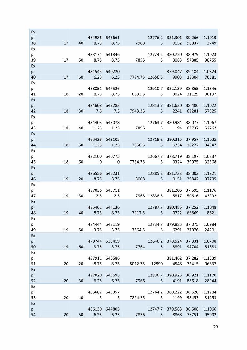
70

Exp 38 17 40

4849868.75

6436618.75 7908

12776.25

381.3010152

39.26698837

1.10192749

Exp 39 17 50

4831718.75

6418468.75 7855

12724.25

380.7203083

38.97957885

1.102398755

Exp 40 17 60

4815456.25

6402206.25 7774.75 12656.5

379.0479903

39.18438304

1.082470581

Exp 41 18 20

4888518.75

6475268.75 8033.5

12910.75

382.1399024

38.86531129

1.134608197

Exp 42 18 30

4846087.5

6432837.5 7943.25

12813.75

381.6302241

38.40662281

1.102257325

Exp 43 18 40

4844031.25

6430781.25 7896

12763.75

380.98494

38.07763737

1.106752762

Exp 44 18 50

4834281.25

6421031.25 7850.5

12718.25

380.3156734

37.95718277

1.103594347

Exp 45 18 60

4821000

6407750 7784.75

12667.75

378.7190324

38.19739075

1.083732368

Exp 46 19 20

4865568.75

6452318.75 8008

12885.25

381.7330151

38.00329842

1.122197795

Exp 47 19 30

4870362.5

6457112.5 7968 12838.5

381.2065817

37.59550616

1.117643292

Exp 48 19 40

4854618.75

6441368.75 7917.5

12787.75

380.4850722

37.25266869

1.10488621

Exp 49 19 50

4844443.75

6431193.75 7864.5

12734.75

379.8856291

37.07527076

1.098424201

Exp 50 19 60

4797443.75

6384193.75 7764

12646.25

378.5248891

37.33194704

1.070851883

Exp 51 20 20

4879118.75

6465868.75 8012.75 12890

381.4624548

37.28272415

1.133906837

Exp 52 20 30

4870206.25

6456956.25 7966

12836.75

380.9254191

36.92188618

1.117028944

Exp 53 20 40

4866825

6453575 7894.25

12764.25

380.2221199

36.62098453

1.128481453

Exp 54 20 50

4861306.25

6448056.25 7876

12747.75

379.5838868

36.50876751

1.106695002

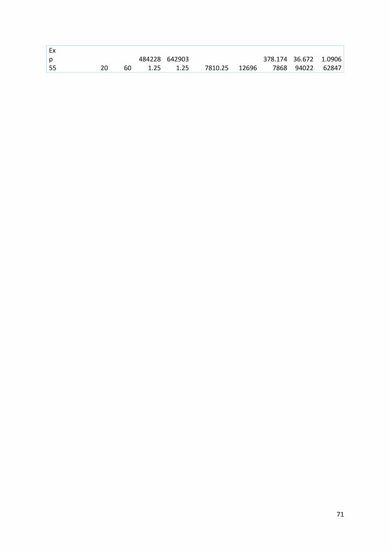
71

Exp 55 20 60

4842281.25

6429031.25 7810.25 12696

378.1747868

36.67294022

1.090662847