Graduate Lecture

Dark Energy - Observational Evidence and

Theoretical Modeling

Lectures I+II

Jochen Weller

Department of Physics & Astronomy

University College London

January 12, 2006

Contents

1 Introduction 2

1.1 Bibliography . . . . . . . . . . . . . . . . . . . . . . . . . . . 2

2 Observational Evidence for Accelerated Expansion from Su-

pernovae 3

2.1 The Luminosity Distance . . . . . . . . . . . . . . . . . . . . 32.1.1 The Robertson-Walker Metric and Friedman Equation 32.1.2 The Critical Density . . . . . . . . . . . . . . . . . . . 42.1.3 Redshift . . . . . . . . . . . . . . . . . . . . . . . . . . 62.1.4 Proper and Angular Diameter Distance . . . . . . . . 72.1.5 Luminosity Distance and Deceleration Parameter . . . 10

2.2 Distance vs. Redshift with Type Ia Supernovae . . . . . . . . 132.2.1 Cosmological Magnitudes . . . . . . . . . . . . . . . . 132.2.2 Type Ia Supernovae as Standardizable Candles – Phillips

Relation . . . . . . . . . . . . . . . . . . . . . . . . . . 152.3 Parameter Estimation . . . . . . . . . . . . . . . . . . . . . . 18

2.3.1 Sampling the Likelihood by a Grid Based Method . . 222.3.2 Joint Likelihoods . . . . . . . . . . . . . . . . . . . . . 25

1

Chapter 1

Introduction

~ = c = k = 1.

1.1 Bibliography

Ray d’Inverno, Introducing Einstein’s Relativity, Oxford University Press.Sean M. Carroll, Spacetime and Geometry, Addison Wesley.Steven Weinberg, Gravitation and Cosmology, Wiley & Sons.Malcolm S. Longair, Galaxy Formation, Springer.Marc L. Kutner, Astronomy: A Physical Perspective, Cambridge UniversityPress.

2

Chapter 2

Observational Evidence for

Accelerated Expansion from

Supernovae

2.1 The Luminosity Distance

2.1.1 The Robertson-Walker Metric and Friedman Equation

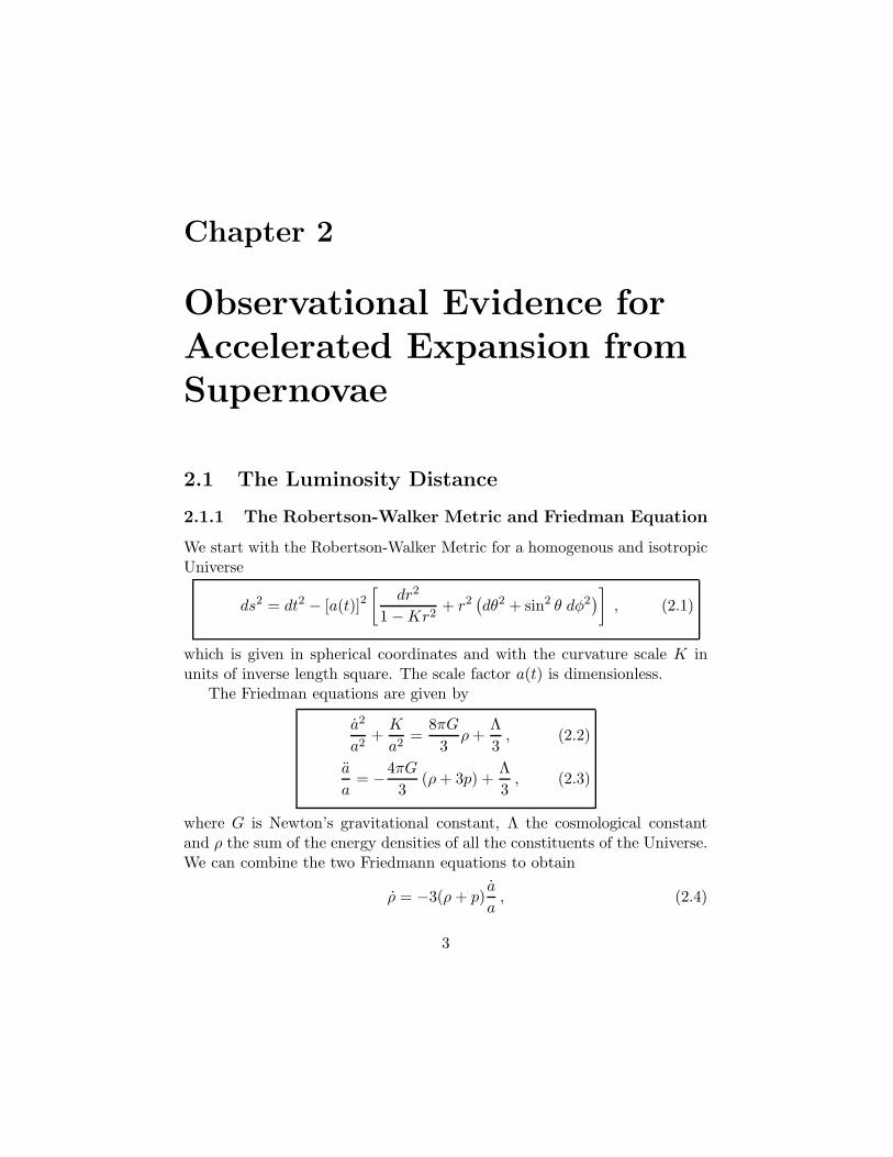
We start with the Robertson-Walker Metric for a homogenous and isotropicUniverse

ds2 = dt2 − [a(t)]2[

dr2

1 − Kr2+ r2

(

dθ2 + sin2 θ dφ2)

]

, (2.1)

which is given in spherical coordinates and with the curvature scale K inunits of inverse length square. The scale factor a(t) is dimensionless.

The Friedman equations are given by

a2

a2+

K

a2=

8πG

3ρ +

Λ

3, (2.2)

a

a= −

4πG

3(ρ + 3p) +

Λ

3, (2.3)

where G is Newton’s gravitational constant, Λ the cosmological constantand ρ the sum of the energy densities of all the constituents of the Universe.We can combine the two Friedmann equations to obtain

ρ = −3(ρ + p)a

a, (2.4)

3

which if we multiply this by a3 and note that the volume V ∝ a3 is theequation for the conservation of energy with

dE + pdV = 0 ,

where we recognise that the pressure does work in the expansion.

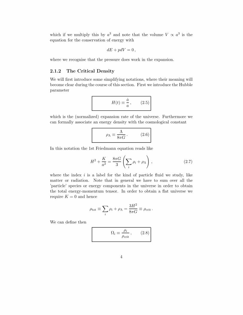
2.1.2 The Critical Density

We will first introduce some simplifying notations, where their meaning willbecome clear during the course of this section. First we introduce the Hubbleparameter

H(t) ≡a

a, (2.5)

which is the (normalized) expansion rate of the universe. Furthermore wecan formally associate an energy density with the cosmological constant

ρΛ ≡Λ

8πG. (2.6)

In this notation the 1st Friedmann equation reads like

H2 +K

a2=

8πG

3

(

∑

i

ρi + ρΛ

)

, (2.7)

where the index i is a label for the kind of particle fluid we study, likematter or radiation. Note that in general we have to sum over all the’particle’ species or energy components in the universe in order to obtainthe total energy-momentum tensor. In order to obtain a flat universe werequire K = 0 and hence

ρtot ≡∑

i

ρi + ρΛ =3H2

8πG≡ ρcrit .

We can define then

Ωi ≡ρi

ρcrit, (2.8)

4

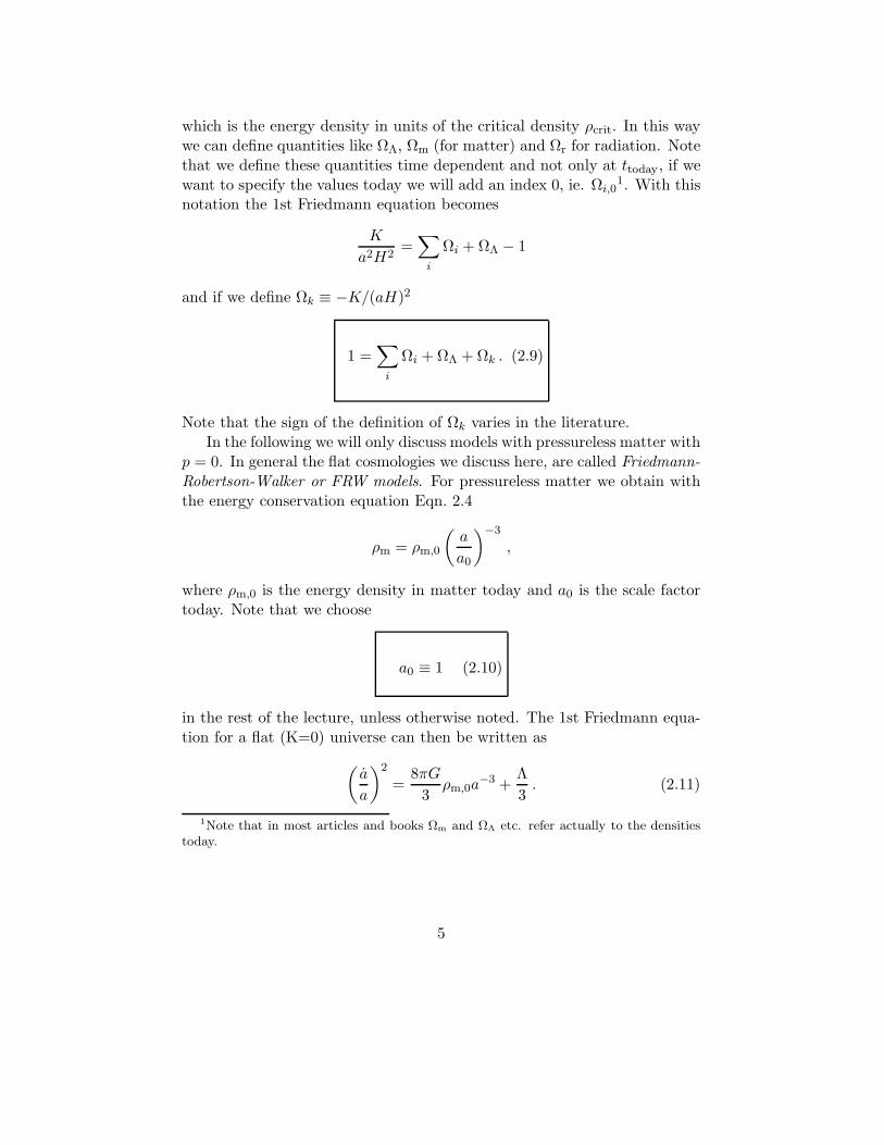
which is the energy density in units of the critical density ρcrit. In this waywe can define quantities like ΩΛ, Ωm (for matter) and Ωr for radiation. Notethat we define these quantities time dependent and not only at ttoday, if wewant to specify the values today we will add an index 0, ie. Ωi,0

1. With thisnotation the 1st Friedmann equation becomes

K

a2H2=∑

i

Ωi + ΩΛ − 1

and if we define Ωk ≡ −K/(aH)2

1 =∑

i

Ωi + ΩΛ + Ωk . (2.9)

Note that the sign of the definition of Ωk varies in the literature.In the following we will only discuss models with pressureless matter with

p = 0. In general the flat cosmologies we discuss here, are called Friedmann-

Robertson-Walker or FRW models. For pressureless matter we obtain withthe energy conservation equation Eqn. 2.4

ρm = ρm,0

(

a

a0

)−3

,

where ρm,0 is the energy density in matter today and a0 is the scale factortoday. Note that we choose

a0 ≡ 1 (2.10)

in the rest of the lecture, unless otherwise noted. The 1st Friedmann equa-tion for a flat (K=0) universe can then be written as

(

a

a

)2

=8πG

3ρm,0a

−3 +Λ

3. (2.11)

1Note that in most articles and books Ωm and ΩΛ etc. refer actually to the densitiestoday.

5

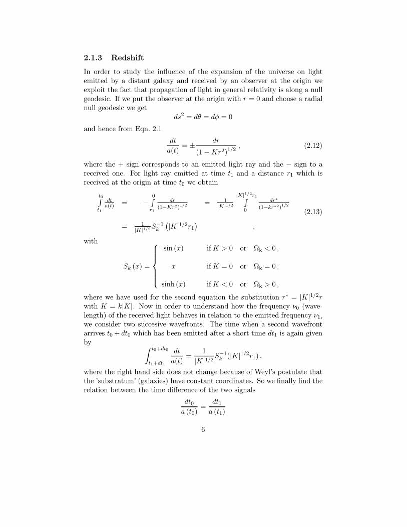
2.1.3 Redshift

In order to study the influence of the expansion of the universe on lightemitted by a distant galaxy and received by an observer at the origin weexploit the fact that propagation of light in general relativity is along a nullgeodesic. If we put the observer at the origin with r = 0 and choose a radialnull geodesic we get

ds2 = dθ = dφ = 0

and hence from Eqn. 2.1

dt

a(t)= ±

dr

(1 − Kr2)1/2, (2.12)

where the + sign corresponds to an emitted light ray and the − sign to areceived one. For light ray emitted at time t1 and a distance r1 which isreceived at the origin at time t0 we obtain

t0∫

t1

dta(t) = −

0∫

r1

dr

(1−Kr2)1/2= 1

|K|1/2

|K|1/2r1∫

0

dr∗

(1−kr∗2)1/2

= 1|K|1/2

S−1k

(

|K|1/2r1

)

,

(2.13)

with

Sk (x) =

sin (x) if K > 0 or Ωk < 0 ,

x if K = 0 or Ωk = 0 ,

sinh (x) if K < 0 or Ωk > 0 ,

where we have used for the second equation the substitution r∗ = |K|1/2rwith K = k|K|. Now in order to understand how the frequency ν0 (wave-length) of the received light behaves in relation to the emitted frequency ν1,we consider two succesive wavefronts. The time when a second wavefrontarrives t0 + dt0 which has been emitted after a short time dt1 is again givenby

∫ t0+dt0

t1+dt1

dt

a(t)=

1

|K|1/2S−1

k (|K|1/2r1) ,

where the right hand side does not change because of Weyl’s postulate thatthe ’substratum’ (galaxies) have constant coordinates. So we finally find therelation between the time difference of the two signals

dt0a (t0)

=dt1

a (t1)

6

0 0(t +dt , 0)

1 1 1(t +dt , r )

lineP’s world

lineO’s world

(t , 0)0

1 1(t , r )

Figure 2.1: Propagation of light rays.

and hence the relation of the emitted (ν1) and received (ν0) frequencies isgiven by

ν0

ν1=

dt1dt0

=a (t1)

a (t0),

which is usually expressed by the redshift parameter

z ≡λ0 − λ1

λ1=

a (t0)

a (t1)− 1 , (2.14)

where λ1 and λ0 are the wavelength corresponding to ν1 and ν0. Light froma distant object is usually redshifted2. Note that if we put the observer att0 today and use a0 = 1 we obtain

a =1

1 + z(2.15)

2.1.4 Proper and Angular Diameter Distance

In general there is a world time and one can define the absolute distancebetween ’substratum’ particles by looking at their position at the same worldtime. If we set dt = dθ = dφ = 0 in Eqn. 2.1 and assume one particle is atthe origin and the other at r1 we obtain as the proper distance

dp = a(t)

∫ r1

0

dr

(1 − Kr2)1/2,

2Note that in a collapsing universe it is actually blueshifted.

7

o P

dpt

Figure 2.2: Distance between two fluid particles.

however this requires a synchronous measurement of the distance which is ofno practical use. One more practical method would be to compare the knownabsolute luminosity of an object with its observed apparent luminosity orthe true diameter with the observed angular diameter.

In this section we consider the second method, while in the next sectionwe will concentrate on the luminosity measurements. We calculate in thefollowing the angular diameter observed at the origin at t = t0 of a lightsource of of true proper diameter D at r = r1 and t = t1. We choose the

δ

D

r=r

r=0

1

Figure 2.3: Angular diameter distance.

coordinate system like in Fig. 2.3. The light travels then on a cone witha half angle θ = δ/2. The proper diameter of the source is then given byEqn. 2.1

D = a(t1)r1δ for δ 1 ,

8

so we obtain for the angular diameter of the source

δ =D

a(t1)r1.

In Euclidean geometry the angular diameter of a source of diameter D at adistance d is δ = D/d, so we define in general the angular diameter distance

dA ≡D ,

δ(2.16)

and hence we can write

dA = a(t1)r1 =r1

1 + z.

Since we are studying the propagation of light r1 is given by Eqns. 2.12-2.13and we obtain

∫ t0

t1

dt

a(t)=

∫ z

0

dz

H(z)=

1

|K|1/2S−1

k (|K|1/2r1) ,

where the first equation was obtained by substituting the time integrationwith a redshift integration and using

dz

dt= −

a

a2= −

H

a.

and we finally obtain with |K|1/2 = H0

√

Ωk,0

dA(z) =1

√

|Ωk|H0(1 + z)Sk

(

H0

√

|Ωk|

∫ z

0

dz

H(z)

)

.

(2.17)

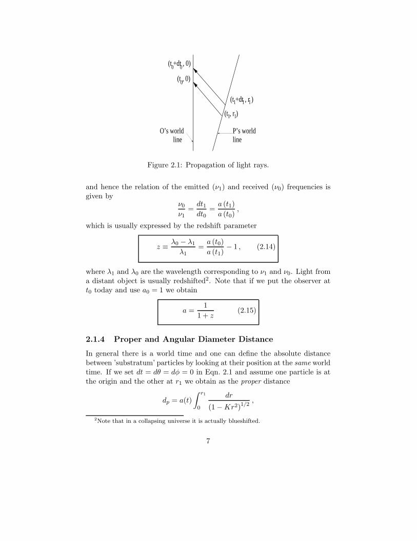
From Eqn. 2.7 we see that the angular diameter distance depends via theHubble parameter on the cosmological parameters like H0, ΩΛ,0 and Ωm,0. Ifon could observe the angular diameter distance really accurately one couldmeasure these parameters and also the curvature or general geometry ofthe universe. An excellent probe in this way in the anisotropies in cosmicmicrowave background radiation. One can calculate a typical size of anoverdense region at the time the microwave photons start to stream freeand we also know the the distance to this last scattering surface. We cancompare this with the observed angular size (in form of the anisotropy powerspectra) and hence obtain a very accurate measurement of the curvature ofthe universe.

9

angular size of typical CMB patch

Figure 2.4: Angular anisotropy power spectrum of the cosmic microwavebackground as observed by the WMAP team (2003).

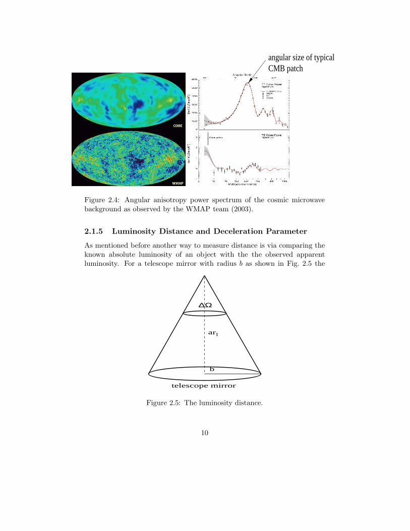
2.1.5 Luminosity Distance and Deceleration Parameter

As mentioned before another way to measure distance is via comparing theknown absolute luminosity of an object with the the observed apparentluminosity. For a telescope mirror with radius b as shown in Fig. 2.5 the

telescope mirror

b

ar

∆Ω

1

Figure 2.5: The luminosity distance.

10

solid angle is given by

∆Ω =πb2

a2(t0)r21

and the fraction of isotropically emitted photons that reach telescope is givenby ratio of solid angle ∆Ω to total solid angle 4π

∆Ω

4π=

πb2

4πa2(t0)r21

If the source has an absolute (or bolometric3) luminosity L, which is thetotal power emitted by the source (in a specified band), the question iswhat is the received power ? Let us look at a single photon. Photonswhich are emitted with energy hν1 are redshifted to hν1a(t1)/a(t0) = hν0.Furthermore photons emitted at intervals δt1 are received at intervals δt0 =δt1a(t0)/a(t1). So for a single photon we get

emitted power : Pem = hν1

δt1

received power : Prec = hν0

δt0

= hν1

δt1

a2(t1)a2(t0)

,

hence for the total received power P , we get

P = L

(

a2(t1)

a2(t0)

)

A

4πa2(t0)r21

,

where we have used A = πb2 for the total mirror area. Now the totalapparent luminosity or bolometric flux density is given by

F ≡P

A=

La2(t1)

4πr21

, (2.18)

where we applied a(t0) = 1. In Euclidean space the flux density is given byF = L/(4πd2) and this is now generalized to define the luminosity distance

3The term bolometric is usually applied when the luminosity is calculated over anentire bandwidth ∆ν.

11

F =L

4πd2L

. (2.19)

Therefore we obtain

dL =r1

a= (1 + z)r1 = (1 + z)2dA ,

so we finally obtain

dL(z) =1 + z

√

|Ωk|H0

Sk

(

H0

√

|Ωk|

∫ z

0

dz

H(z)

)

. (2.20)

It is interesting to note that for low redshifts z 1 and small r1 we have

dA ' dL ' dP ' r1

and the distinction becomes important only for objects billions of light yearsaway. Therefore we draw our attention to the redshift dependence of thescale factor at late times (or small redshifts). We can Taylor expand thescale factor around t = t0 and obtain

a(t) = a(t0)

[

1 + H0 (t − t0) −1

2q0H

20 (t0 − t)2 + · · ·

]

, (2.21)

where we used the definition of the Hubble constant H0 = a(t0)/a(t0) andwe defined the deceleration parameter

q0 = −a(t0)

a(t0)H20

. (2.22)

As the name already suggests the deceleration parameter quantifies if theexpansion of the universe is accelerating (q0 < 0) or decelerating (q0 > 0).It is quite convenient to express the cosmological models in terms of q0 andH0 but we leave this as an Exercise ! .

If we use this expansion in Eqn. 2.12 for the propagation of light weobtain on for left hand side

∫ t0

t1

dt

a(t)=

1

a(t0)

∫ t0

t1

[

1 + H0(t0 − t) +(

1 +q0

2

)

H20 (t0 − t)2 + · · ·

]

12

and for the right hand side

∫ r1

0

dr

(1 − Kr2)1/2≈

1

|K|1/2

∫ |K|1/2r1

0

(

1 +1

2kr∗2

)

dr∗ = r1 + O(r31)

and we obtain

r1 =1

a(t0)

[

t0 − t1 +1

2H0 (t0 − t1)

2 + · · ·

]

.

Furthermore we obtain for the redshift

z =1

a− 1 = H0(t0 − t1) +

(

1 +q0

2

)

H20 (t0 − t1)

2 + · · ·

and hence

r1 =1

a(t0)H0

[

z −1

2(1 + q0) z2 + · · ·

]

.

Finally we can write the expansion of the luminosity distance for low red-shifts

dL = H−10

[

z +1

2(1 − q0) z2 + · · ·

]

. (2.23)

This expansion will play a vital role for the calibration of the magnitude -redshift relation for Supernovae as we will discuss it in Section 2.2.

2.2 Distance vs. Redshift with Type Ia Super-

novae

We will now study an application of what we have learned so far. Theanalysis of the distance - redshift relation with Type Ia Supernovae and thewhat we can learn about the cosmological parameters H0, ΩΛ,0, Ωm,0 andΩk,0.

However in order to do this we need to introduce the notion of magni-tudes.

2.2.1 Cosmological Magnitudes

When we discussed the luminosity distance in Section 2.1.5 we introducedthe notion of of bolometric flux, which is related to the bolometric brightness.The brightness in general is the intensity of a radiating source, ie. the energyflux per solid angle and per unit frequency. The bolometric brightness againis integrated over a frequency wave band. Now the definition of magnitudes

13

is an ancient concept. Hipparchus (150 BC) divided stars into six classesof brightness he called magnitudes. The brightest stars were called firstmagnitude and the faintest sixth. With quantitative measurements it wasfound that each jump in magnitude corresponded to a fixed ratio in flux,hence the magnitude scale is logarithmic. This is not too surprising sincethe eye has an approximately logarithmic response to light, which enablesa large dynamic range. It was found that a difference of five magnitudescorresponds to a factor 100 in brightness and we have

b

B= 100(M−m)/5 = 10(m2−m1)/2.5 .

Instead of using the brightness ratio we could have also used the ratio of thereceived flux. We can now build up the magnitude ladder with a standardcandle. A standard candle is an object which has always the same emittedluminosity L. We obtain then with Eqn. 2.18

M − m = 2.5 logd2L,0

d2L

= 5 logdL,0

dL,

where M is the intrinsic magnitude of the standard candle at some close bydistance dL,0. In astronomical situations this distance is usually chosen to10 pc4. So usually one obtains

m = M + 5 log dL .

where dL is given in units of 10 pc. However in cosmological situation thisis a rather small distance and a more natural unit is 1Mpc. If we measurethe distance in this unit the apparent magnitude is given by

m = M + 5 log dL + 25 . (2.24)

If we use the approximation for z 1 for the luminosity distance inEqn. 2.23 we obtain

m = M − 5 log H0 + 5 log cz + · · · + 25 . (2.25)

Note that we explicitly write the speed of light c in this equation. Thisapproximation only depends on the Hubble constant H0 but not on othercosmological parameters. So nearby objects can be used to calibrate for theintrinsic magnitude M .

4The unit 1 pc is defined to be the distance of an object which produces one arcsec ofa parallax angle for one astronomical unit (AU), which is the distance from the sun to theearth. 1 pc = 3.09 × 1016 m.

14

2.2.2 Type Ia Supernovae as Standardizable Candles – Phillips

Relation

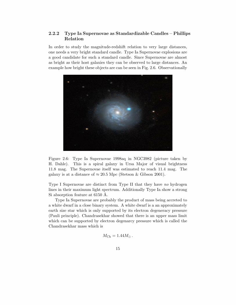
In order to study the magnitude-redshift relation to very large distances,one needs a very bright standard candle. Type Ia Supernovae explosions area good candidate for such a standard candle. Since Supernovae are almostas bright as their host galaxies they can be observed to large distances. Anexample how bright these objects are can be seen in Fig. 2.6. Observationally

Figure 2.6: Type Ia Supernovae 1998aq in NGC3982 (picture taken byH. Dahle). This is a spiral galaxy in Ursa Major of visual brightness11.8 mag. The Supernovae itself was estimated to reach 11.4 mag. Thegalaxy is at a distance of ≈ 20.5 Mpc (Stetson & Gibson 2001).

Type I Supernovae are distinct from Type II that they have no hydrogenlines in their maximum light spectrum. Additionally Type Ia show a strongSi absorption feature at 6150 A.

Type Ia Supernovae are probably the product of mass being accreted toa white dwarf in a close binary system. A white dwarf is a an approximatelyearth size star which is only supported by its electron degeneracy pressure(Pauli principle). Chandrasekhar showed that there is an upper mass limitwhich can be supported by electron degenarcy pressure which is called theChandrasekhar mass which is

MCh = 1.44M .

15

Sometimes there is too much mass accreted onto the white dwarf and itsstarts to exceed the Chandrasekhar mass limit. In this case the degener-ate electron pressure can no longer support the star and it collapses. Thecollapse energy drives nuclear reaction which build up 56Ni which β-decaysinto 56Co which in turn β-decays into 56Fe.

Figure 2.7: Model of close binary system which might be the progenitor toa Type Ia Supernovae explosion [Picture take from Paul Rickers web page].

These thermonuclear explosions lead to typical typical brightening andfading of the Supernovae, which in case of the Type Ia is governed by atwo exponential whose timescale is governed by the two β-decays. Note thethe β-decay of 56Ni has a halftime of τNi = 17.6 days. In Fig. 2.8 we seea typical SNe observation, where the discovery was made from the groundand the follow up with the Hubble Space Telescope. The brightening andfading gives rise to a typical lightcurve for Type Ia Supernovae as shown inFig. 2.9. One problem with Type Ia SNe is however that, although they havea narrow range of absolute peak magnitudes M , there is a slight variation.

However Phillips (1993) discovered that there is a tight relation betweenthe peak magnitude and the decay time. This relation is not well understoodyet from a theoretical point of view but basically the time scale and theoverall energy of the Supernovae explosion depend both on the amount ofNi which is present in the progenitor. With the Phillips relation it is possibleto normalize the peak flux and also “stretch” the time axis so that all Type Ia

16

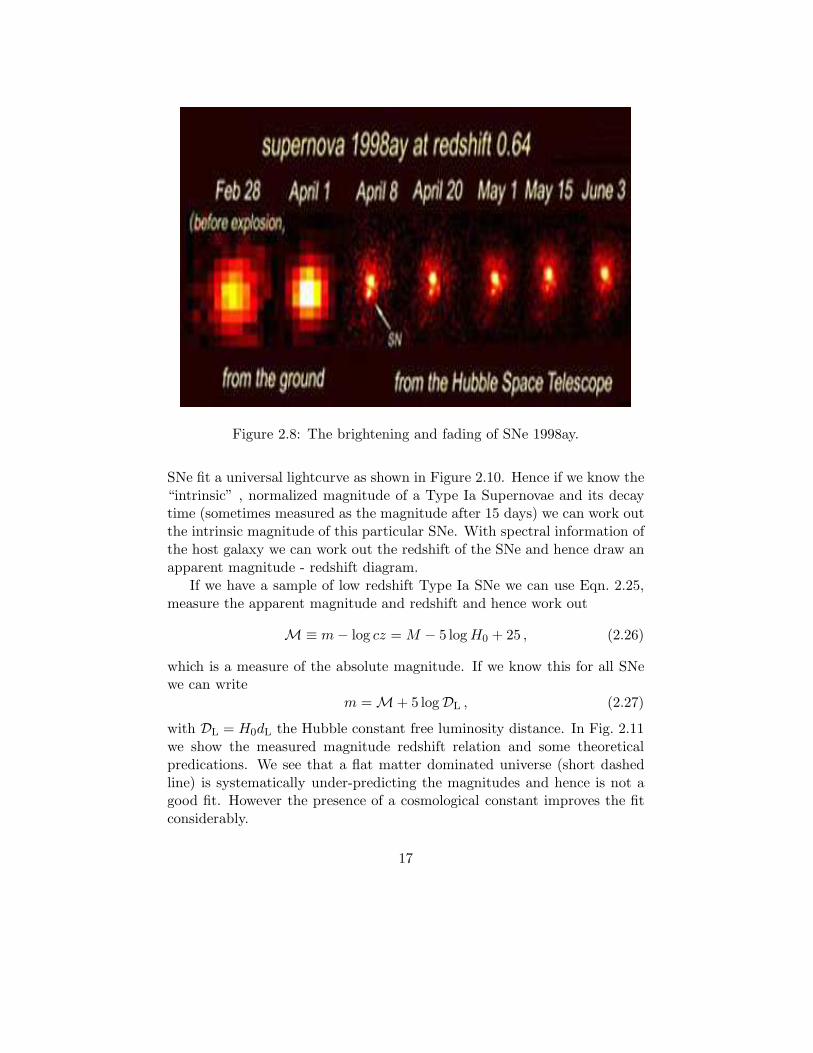
Figure 2.8: The brightening and fading of SNe 1998ay.

SNe fit a universal lightcurve as shown in Figure 2.10. Hence if we know the“intrinsic” , normalized magnitude of a Type Ia Supernovae and its decaytime (sometimes measured as the magnitude after 15 days) we can work outthe intrinsic magnitude of this particular SNe. With spectral information ofthe host galaxy we can work out the redshift of the SNe and hence draw anapparent magnitude - redshift diagram.

If we have a sample of low redshift Type Ia SNe we can use Eqn. 2.25,measure the apparent magnitude and redshift and hence work out

M ≡ m − log cz = M − 5 log H0 + 25 , (2.26)

which is a measure of the absolute magnitude. If we know this for all SNewe can write

m = M + 5 logDL , (2.27)

with DL = H0dL the Hubble constant free luminosity distance. In Fig. 2.11we show the measured magnitude redshift relation and some theoreticalpredications. We see that a flat matter dominated universe (short dashedline) is systematically under-predicting the magnitudes and hence is not agood fit. However the presence of a cosmological constant improves the fitconsiderably.

17

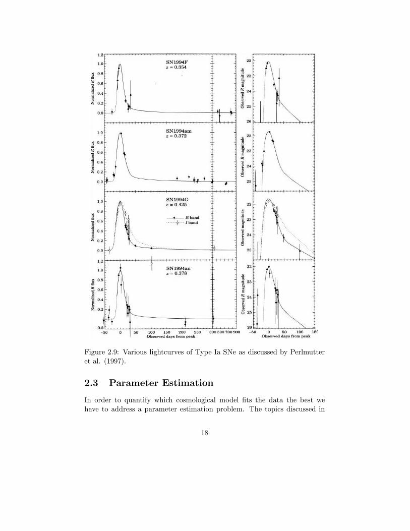
Figure 2.9: Various lightcurves of Type Ia SNe as discussed by Perlmutteret al. (1997).

2.3 Parameter Estimation

In order to quantify which cosmological model fits the data the best wehave to address a parameter estimation problem. The topics discussed in

18

Figure 2.10: Stretch factor corrected lightcurves from SCP.

this Section apply in general for the estimation of parameters and are hencea valuable tool for every physicist who has to deal with data.

Let us assume that we have a sample of Type Ia SNe with a given mag-nitude mi and uncertainty in the magnitude σm,i, which is typically of theorder σm = 0.15 mag. Furthermore we know the redshift zi of the Su-

19

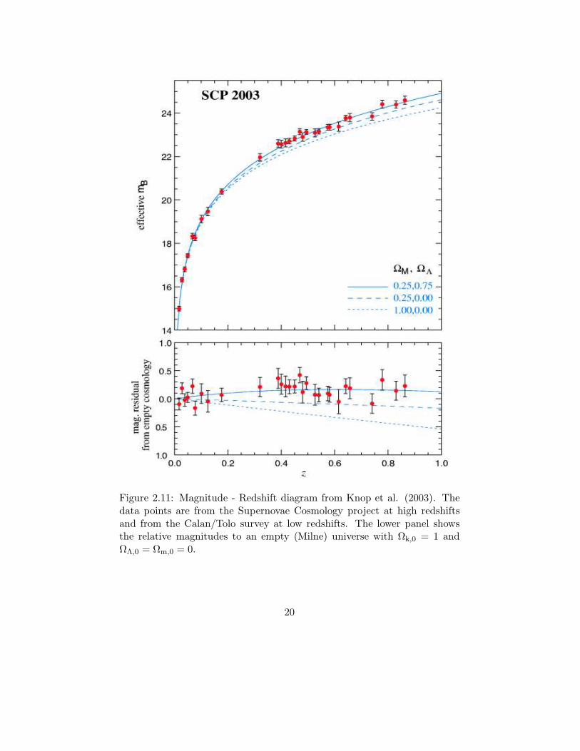
Figure 2.11: Magnitude - Redshift diagram from Knop et al. (2003). Thedata points are from the Supernovae Cosmology project at high redshiftsand from the Calan/Tolo survey at low redshifts. The lower panel showsthe relative magnitudes to an empty (Milne) universe with Ωk,0 = 1 andΩΛ,0 = Ωm,0 = 0.

20

pernovae. In general this redshift has an errorbar as well, but it can beneglected in comparison to the magnitude uncertainty. We can than com-pare the measurement with the theoretical prediction of Eqn. 2.27 for eachset of parameters (Ωm,0,ΩΛ,0,M). There are two ways to tackle the absolutemagnitude M. We could first just look at the low redshift SNe sample fromCalan/Tololo and use Eqn. 2.26 to measure the absolute magnitude. Notethat this equation does not depend on the cosmological parameters. Sec-ondly we could view M as a free parameter like the cosmological parameters(Ωm,0,ΩΛ,0) and try to find the best fit value for it.

We will follow the second approach here. In order to get a compactnotation we define the parameter vector

θ ≡ (Ωm,0,ΩΛ,0,M) .

If we assume that the errors in the magnitude follow a Gaussian distri-bution we can obtain the best fit parameters by maximising the posteriorprobability (likelihood)

L(θ) ∝ exp

[

−1

2χ2

]

with

χ2 =

N∑

i=1

(

m(zi; θ) − mi

σm,i

)2

,

where N is the number of data points. One can then numerically minimizeEqn. 2.3 and obtain the best fit values θ. As a matter of fact by calculat-ing L(θ) over the entire sensible parameter range we obtain the posteriordistribution.

Since from a cosmological point of view we are not interested in the abso-lute magnitude M we can marginalize over it and obtain the 2-dimensionalprobability distribution

L(Ωm,0,ΩΛ,0) =

∫

dM L(Ωm,0,ΩΛ,0,M) .

In fact this can be even done analytically because M is just a linearly addedparameter. If we define

c1 ≡N∑

i=1

1

σ2m,i

f0 ≡

N∑

i=1

5 logDL(zi) − mi

σ2m,i

21

f1 ≡

N∑

i=1

(5 logDL(zi) − mi)2

σ2m,i

,

we obtain

χ2 = f1 −f20

c1(2.28)

2.3.1 Sampling the Likelihood by a Grid Based Method

We start with a Fortran 90 example of how to calculate the χ2 values.

MODULE STATISTICS

CONTAINS

! calculate standard chi2 function

FUNCTION CHI2(omegami,omegali,Minti)

USE COSMOLOGY

USE SNDATA

REAL, INTENT(IN) :: omegami,omegali,Minti

INTEGER :: I

REAL :: sum

REAL :: CHI2

omegam=omegami

omegal=omegali

Mint=Minti

omegak=1.0-omegam-omegal

IF (NOB(omegam,omegal)) THEN

sum = 0.0

DO I=1,N

sum=sum+(m(i)-mag(z(i)))**2/dm(i)**2

END DO

CHI2 = sum

ELSE

CHI2 = 1.0E30 ! assign zero likelihood if nobtest fails

END IF

RETURN

END FUNCTION CHI2

! calculate chi2 function; with analytic marginalization over Mint

22

FUNCTION CHI2ANA(omegami,omegali)

USE COSMOLOGY

USE SNDATA

REAL, INTENT(IN) :: omegami,omegali

INTEGER :: I

REAL :: c1,f0,f1

REAL :: CHI2ANA

omegam=omegami

omegal=omegali

Mint=0.0 ! note we set this zero in order to calc 5.0*log(DL)

omegak=1.0-omegam-omegal

IF (NOB(omegam,omegal)) THEN

c1=0.0

f0=0.0

f1=0.0

DO I=1,N

c1=c1+1.0/dm(i)**2

f0=f0+(mag(z(i))-m(i))/dm(i)**2

f1=f1+(mag(z(i))-m(i))**2/dm(i)**2

END DO

CHI2ANA = f1-f0*f0/c1

ELSE

CHI2ANA = 1.0E30 ! assign zero likelihood if nobtest fails

END IF

RETURN

END FUNCTION CHI2ANA

END MODULE STATISTICS

The likelihood is simply calculated by looping over the parameters andcalculating the χ2 values for each grid point. The function CHI2 calculatesthe χ2 in the classical way, while CHI2ANA is using the analytical marginal-ization over the intrinsic magnitude M. The function mag(z) calculates thetheoretical magnitudes for a given model, the arrays z(i), m(i) and dm(i)

hold the data points. Also note the logical function NOB, which sorts out themodels for which no big bang occurs which are given by the condition

ΩΛ,0 ≥ 4Ωm,0

coss

[

1

3coss−1

(

1 − Ωm,0

Ωm,0

)]3

, (2.29)

with “coss” being defined as cosh for Ωm,0 < 1/2 and cos for Ωm,0 > 1/2. Ifthis condition is fullfilled, the argument in the square root of the definition

23

of the Hubble parameter can become negativ for certain redshifts. We hencejust assign a zero likelihood for these models. We can now discuss how weloop over the different parameters:

DO OMEGAM = 0.0,1.5,0.1

DO OMEGAL = -1.0,2.0,0.1

omegak = 1.0-omegam-omegal

DO Mint = 15.5,16.5,0.01

test=chi2(omegam,omegal,Mint)

write(11,FMT=’(3F10.2,F18.10)’) Mint,OMEGAM,OMEGAL,exp(-0.5*(test-testmin))

! FIND MINIMUM

if (test<chi2min) then

chi2min=test

omegammin = omegam

omegalmin = omegal

Mintmin = Mint

END IF

END DO

END DO

END DO

and for the analytically marginalized fit:

DO OMEGAM = 0.0,1.5,0.1

DO OMEGAL = -1.0,2.0,0.1

omegak = 1.0-omegam-omegal

test=chi2ana(omegam,omegal)

write(11,FMT=’(2F10.2,F18.10)’) OMEGAM,OMEGAL,exp(-0.5*(test-testmin))

! FIND MINIMUM

if (test<chi2min) then

chi2min=test

omegammin = omegam

omegalmin = omegal

END IF

END DO

write(11,*)

END DO

24

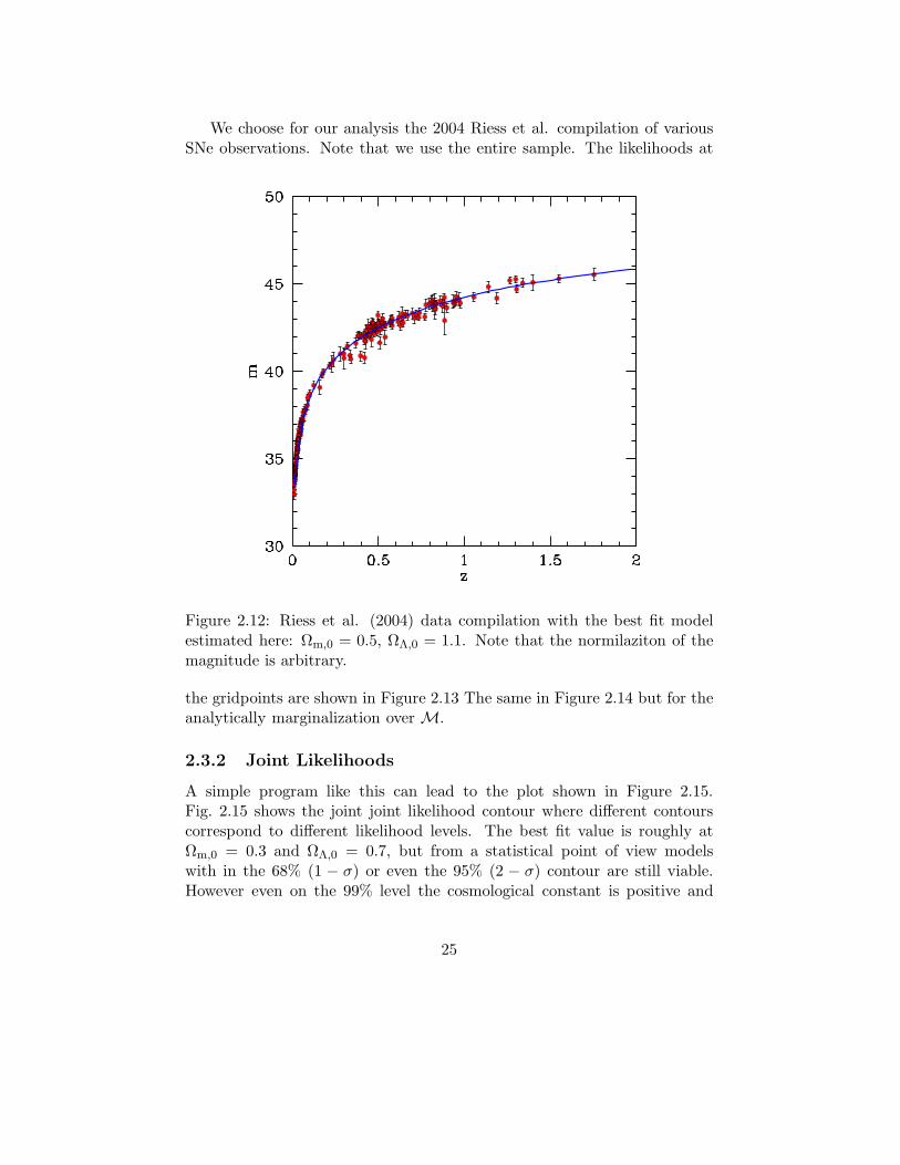
We choose for our analysis the 2004 Riess et al. compilation of variousSNe observations. Note that we use the entire sample. The likelihoods at

Figure 2.12: Riess et al. (2004) data compilation with the best fit modelestimated here: Ωm,0 = 0.5, ΩΛ,0 = 1.1. Note that the normilaziton of themagnitude is arbitrary.

the gridpoints are shown in Figure 2.13 The same in Figure 2.14 but for theanalytically marginalization over M.

2.3.2 Joint Likelihoods

A simple program like this can lead to the plot shown in Figure 2.15.Fig. 2.15 shows the joint joint likelihood contour where different contourscorrespond to different likelihood levels. The best fit value is roughly atΩm,0 = 0.3 and ΩΛ,0 = 0.7, but from a statistical point of view modelswith in the 68% (1 − σ) or even the 95% (2 − σ) contour are still viable.However even on the 99% level the cosmological constant is positive and

25

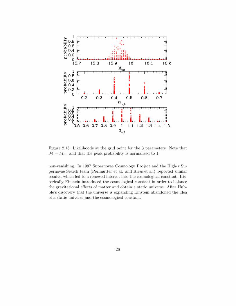
Figure 2.13: Likelihoods at the grid point for the 3 parameters. Note thatM = Mint and that the peak probability is normalized to 1.

non-vanishing. In 1997 Supernovae Cosmology Project and the High-z Su-pernovae Search team (Perlmutter et al. and Riess et al.) reported similarresults, which led to a renewed interest into the cosmological constant. His-torically Einstein introduced the cosmological constant in order to balancethe gravitational effects of matter and obtain a static universe. After Hub-ble’s discovery that the universe is expanding Einstein abandoned the ideaof a static universe and the cosmological constant.

26

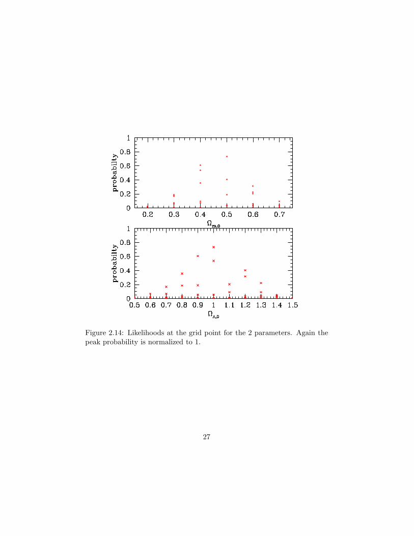
Figure 2.14: Likelihoods at the grid point for the 2 parameters. Again thepeak probability is normalized to 1.

27

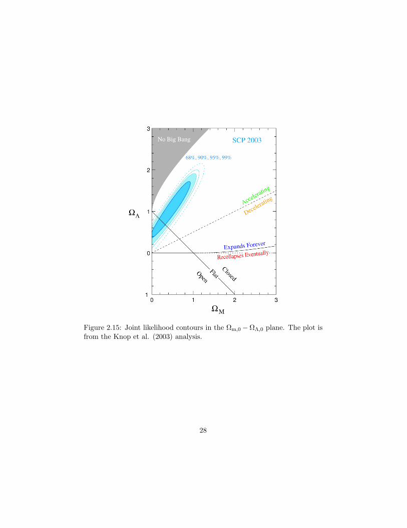
Figure 2.15: Joint likelihood contours in the Ωm,0 −ΩΛ,0 plane. The plot isfrom the Knop et al. (2003) analysis.

28