GPU Cluster Computing for Finite Element … Cluster Computing for Finite Element Applications...

1

GPU Cluster Computingfor Finite Element Applications

Dominik Goddeke, Hilmar Wobker,Sven H.M. Buijssen and Stefan Turek

Applied MathematicsTU Dortmund

[email protected]://www.mathematik.tu-dortmund.de/~goeddeke

38th SPEEDUP Workshop on High-Performance ComputingEPF Lausanne, Switzerland, September 7, 2009

[email protected]

http://www.mathematik.tu-dortmund.de/~goeddeke

2

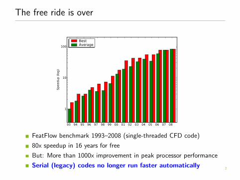
The free ride is over

93 94 95 96 97 98 99 00 01 02 03 04 05 06 07 08

1

10

100

Speedup (

log)

BestAverage

FeatFlow benchmark 1993–2008 (single-threaded CFD code)

80x speedup in 16 years for free

But: More than 1000x improvement in peak processor performance

Serial (legacy) codes no longer run faster automatically

3

Outline

1 FEAST – hardware-oriented numerics

2 Precision and accuracy

3 Co-processor integration

4 Results

5 Conclusions

4

FEAST –

Hardware-oriented Numerics

5

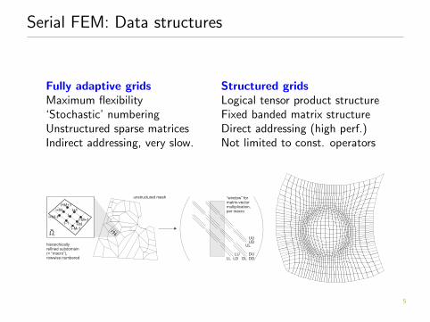
Serial FEM: Data structures

Fully adaptive gridsMaximum flexibility‘Stochastic’ numberingUnstructured sparse matricesIndirect addressing, very slow.

Structured gridsLogical tensor product structureFixed banded matrix structureDirect addressing (high perf.)Not limited to const. operators

UU

“window” formatrix-vectormultiplication,per macro

hierarchicallyrefined subdomain(= “macro”),rowwise numbered

unstructured mesh

UDUL

DUDDDL

LULDLL

I-1

I

I+1

I-M-1I-M

I-M+1I+M-1

I+M

I+M+1

Ωi

6

Example: SpMV on TP grid

0

500

1000

1500

2000

2500

3000

652 1292 2572 5122 10252

----

> la

rger

is b

ette

r --

-->

MF

LOP

/s fo

r S

pMV

CSR, 2-levelCSR, Cuthill-McKee

CSR, XYZCSR, Stochastic

CSR, HierarchicalBanded

Banded-const

Opteron 2214 dual-core, 2.2 GHz, 2x1 MB L2 cache, one thread

50 vs. 550 MFLOP/s for interesting large problem size

Cache-aware implementation ⇒ 90% of memory throughput

const: Stencil-based computation

7

Serial FEM: Solvers

CG (simple) CG (advanced) MG (simple) MG (advanced)

1

10

100

1000

2000

Speedup (

log)

CG (simple) CG (advanced) MG (simple) MG (advanced)

1

10

100

1000

2000StochasticXYZBanded

More than 1300x faster due to hardware-oriented numerics

8

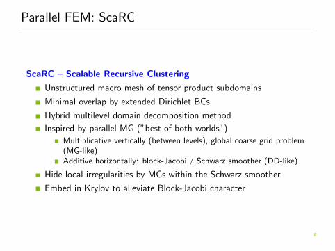
Parallel FEM: ScaRC

ScaRC – Scalable Recursive Clustering

Unstructured macro mesh of tensor product subdomains

Minimal overlap by extended Dirichlet BCs

Hybrid multilevel domain decomposition method

Inspired by parallel MG (”best of both worlds”)

Multiplicative vertically (between levels), global coarse grid problem(MG-like)Additive horizontally: block-Jacobi / Schwarz smoother (DD-like)

Hide local irregularities by MGs within the Schwarz smoother

Embed in Krylov to alleviate Block-Jacobi character

9

Parallel FEM: Solver template

Generic ScaRC solver template for scalar elliptic PDEs

global BiCGStab

preconditioned by

global multigrid (V 1+1)

additively smoothed by

for all Ωi: local multigrid

coarse grid solver: UMFPACK

10

Multivariate problems

Block-structured systems

Guiding idea: Tune scalar case once per architecture instead of overand over again per application

Equation-wise ordering of the unknowns

Block-wise treatment enables multivariate ScaRC solvers

Examples

Linearised elasticity with compressible material

Saddle point problems: Stokes, elasticity with (nearly)incompressible material, Navier-Stokes with stabilisation

(

A11 A12A21 A22

)(

u1u2

)

= f,

A11 0 B10 A22 B2

BT1 BT

2 0

v1v2p

= f,

A11 A12 B1A21 A22 B2

BT1 BT

2 CC

v1v2p

= f

A11 and A22 correspond to scalar elliptic operators⇒ Tuned linear algebra (and tuned solvers)

11

Precision vs. accuracy

Mixed precision methods

12

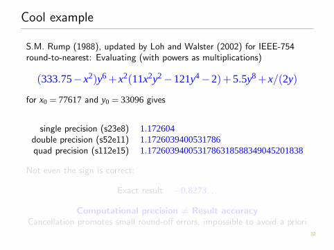
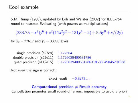
Cool example

S.M. Rump (1988), updated by Loh and Walster (2002) for IEEE-754round-to-nearest: Evaluating (with powers as multiplications)

(333.75− x2)y6 + x2(11x2y2 −121y4 −2)+5.5y8 + x/(2y)

for x0 = 77617 and y0 = 33096 gives

single precision (s23e8) 1.172604double precision (s52e11) 1.1726039400531786quad precision (s112e15) 1.1726039400531786318588349045201838

Not even the sign is correct:

Exact result −0.8273 . . .

Computational precision 6= Result accuracyCancellation promotes small round-off errors, impossible to avoid a priori

13

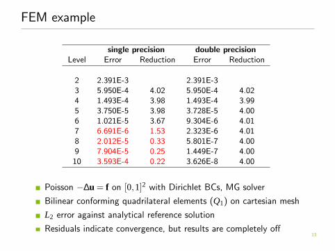
FEM example

single precision double precisionLevel Error Reduction Error Reduction

2 2.391E-3 2.391E-33 5.950E-4 4.02 5.950E-4 4.024 1.493E-4 3.98 1.493E-4 3.995 3.750E-5 3.98 3.728E-5 4.006 1.021E-5 3.67 9.304E-6 4.017 6.691E-6 1.53 2.323E-6 4.018 2.012E-5 0.33 5.801E-7 4.009 7.904E-5 0.25 1.449E-7 4.0010 3.593E-4 0.22 3.626E-8 4.00

Poisson −∆u = f on [0,1]2 with Dirichlet BCs, MG solver

Bilinear conforming quadrilateral elements (Q1) on cartesian mesh

L2 error against analytical reference solution

Residuals indicate convergence, but results are completely off

14

Mixed precision motivation

Bandwidth bound algorithms

64 bit = 1 double = 2 floats

More variables per bandwidth (comp. intensity up)

More variables per storage (data block size up)

Applies to all memory levels:disc ⇒ main ⇒ device ⇒ cache ⇒ register

Compute bound algorithms

1 double multiplier ≈ 4 float multipliers (quadratic)

1 double adder ≈ 2 float adders (linear)

Multipliers are much bigger than adders⇒ Quadrupled computational efficiency

15

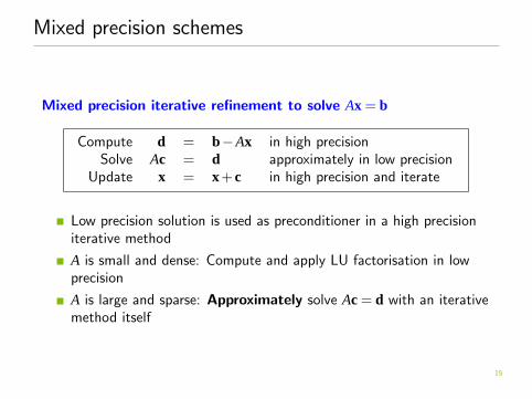
Mixed precision schemes

Mixed precision iterative refinement to solve Ax = b

Compute d = b−Ax in high precisionSolve Ac = d approximately in low precision

Update x = x+ c in high precision and iterate

Low precision solution is used as preconditioner in a high precisioniterative method

A is small and dense: Compute and apply LU factorisation in lowprecision

A is large and sparse: Approximately solve Ac = d with an iterativemethod itself

16

Co-processor integrationinto FEAST

17

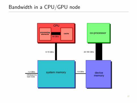
Bandwidth in a CPU/GPU node

18

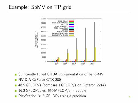
Example: SpMV on TP grid

0

5000

10000

15000

20000

25000

30000

35000

40000

45000

50000

652 1292 2572 5122 10252

----

> la

rger

is b

ette

r --

-->

MF

LOP

/s fo

r S

pMV

CSR, 2-levelCSR, Cuthill-McKee

CSR, XYZCSR, Stochastic

CSR, HierarchicalBanded

Banded-constBanded-GPU single

Banded-GPU double

Sufficiently tuned CUDA implementation of band-MV

NVIDIA GeForce GTX 280

46.5 GFLOP/s (compare 1 GFLOP/s on Opteron 2214)

16.2 GFLOP/s vs. 550 MFLOP/s in double

PlayStation 3: 3 GFLOP/s single precision

19

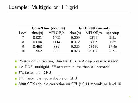
Example: Multigrid on TP grid

Core2Duo (double) GTX 280 (mixed)Level time(s) MFLOP/s time(s) MFLOP/s speedup

7 0.021 1405 0.009 2788 2.3x8 0.094 1114 0.012 8086 7.8x9 0.453 886 0.026 15179 17.4x10 1.962 805 0.073 21406 26.9x

Poisson on unitsquare, Dirichlet BCs, not only a matrix stencil

1M DOF, multigrid, FE-accurate in less than 0.1 seconds!

27x faster than CPU

1.7x faster than pure double on GPU

8800 GTX (double correction on CPU): 0.44 seconds on level 10

20

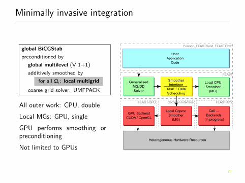
Minimally invasive integration

global BiCGStab

preconditioned by

global multilevel (V 1+1)

additively smoothed by

for all Ωi: local multigrid


All outer work: CPU, double

Local MGs: GPU, single

GPU performs smoothing orpreconditioning

Not limited to GPUs

21

Minimally invasive integration

General approach

Balance acceleration potential and integration effort

Accelerate many different applications built on top of one central FEand solver toolkit

Diverge code paths as late as possible

No changes to application code!

Retain all functionality

Do not sacrifice accuracy

Challenges

Heterogeneous task assignment to maximise throughput

Limited device memory (modeled as huge L3 cache)

Overlapping CPU and GPU computations

Building dense accelerated clusters

22

Some results

23

Linearised elasticity

(

A11 A12A21 A22

)(

u1u2

)

= f

(

(2µ +λ )∂xx + µ∂yy (µ +λ )∂xy

(µ +λ )∂yx µ∂xx +(2µ +λ )∂yy

)

global multivariate BiCGStabblock-preconditioned by

Global multivariate multilevel (V 1+1)additively smoothed (block GS) by

for all Ωi: solve A11c1 = d1 bylocal scalar multigrid

update RHS: d2 = d2 −A21c1

for all Ωi: solve A22c2 = d2 bylocal scalar multigrid


24

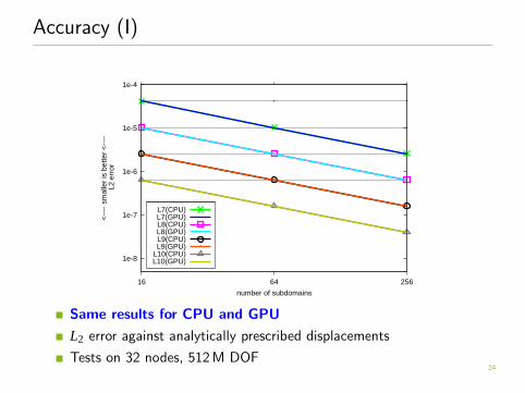
Accuracy (I)

1e-8

1e-7

1e-6

1e-5

1e-4

16 64 256

<--

-- s

mal

ler

is b

ette

r <

----

L2

erro

r

number of subdomains

L7(CPU)L7(GPU)L8(CPU)L8(GPU)L9(CPU)L9(GPU)

L10(CPU)L10(GPU)

Same results for CPU and GPU

L2 error against analytically prescribed displacements

Tests on 32 nodes, 512 M DOF

25

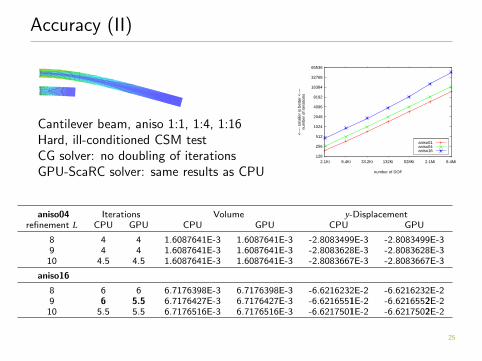
Accuracy (II)

Cantilever beam, aniso 1:1, 1:4, 1:16Hard, ill-conditioned CSM testCG solver: no doubling of iterationsGPU-ScaRC solver: same results as CPU

128

256

512

1024

2048

4096

8192

16384

32768

65536

2.1Ki 8.4Ki 33.2Ki 132Ki 528Ki 2.1Mi 8.4Mi

<--

-- s

mal

ler

is b

ette

r <

----

num

ber

of it

erat

ions

number of DOF

aniso01aniso04aniso16

aniso04 Iterations Volume y-Displacementrefinement L CPU GPU CPU GPU CPU GPU

8 4 4 1.6087641E-3 1.6087641E-3 -2.8083499E-3 -2.8083499E-39 4 4 1.6087641E-3 1.6087641E-3 -2.8083628E-3 -2.8083628E-310 4.5 4.5 1.6087641E-3 1.6087641E-3 -2.8083667E-3 -2.8083667E-3

aniso16

8 6 6 6.7176398E-3 6.7176398E-3 -6.6216232E-2 -6.6216232E-29 6 5.5 6.7176427E-3 6.7176427E-3 -6.6216551E-2 -6.6216552E-210 5.5 5.5 6.7176516E-3 6.7176516E-3 -6.6217501E-2 -6.6217502E-2

26

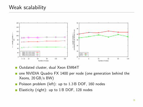
Weak scalability

0

20

40

60

80

100

120

140

160

8 16 32 64 96 128 160

<--

-- s

mal

ler

is b

ette

r <

----

sec

Number of nodes

2c8m_Cn_L10_const1g8m_Cn_L10_const1c8m_Cn_L10_const

20

25

30

35

40

45

50

4 8 16 32 64 128

<--

-- s

mal

ler

is b

ette

r <

----

nor

mal

ized

tim

e pe

r ite

ratio

n in

sec

Number of nodes

CPUGPU

Outdated cluster, dual Xeon EM64T

one NVIDIA Quadro FX 1400 per node (one generation behind theXeons, 20 GB/s BW)

Poisson problem (left): up to 1.3 B DOF, 160 nodes

Elasticity (right): up to 1 B DOF, 128 nodes

27

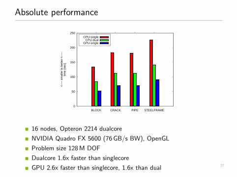
Absolute performance

0

50

100

150

200

250

BLOCK CRACK PIPE STEELFRAME

<--

-- s

mal

ler

is b

ette

r <

----

time

(sec

)

CPU-singleCPU-dual

GPU-single

16 nodes, Opteron 2214 dualcore

NVIDIA Quadro FX 5600 (76 GB/s BW), OpenGL

Problem size 128 M DOF

Dualcore 1.6x faster than singlecore

GPU 2.6x faster than singlecore, 1.6x than dual

28

Acceleration analysis

Speedup analysis

Addition of GPUs increases resources

⇒ Correct model: strong scalability inside each node

Accelerable fraction of the elasticity solver: 2/3

Remaining time spent in MPI and the outer solver

Accelerable fraction Racc: 66%Local speedup Slocal: 9xTotal speedup Stotal: 2.6xTheoretical limit Smax: 3x

1

1.5

2

2.5

3

3.5

4

1 2 3 4 5 6 7 8 9 10

----

> la

rger

is b

ette

r --

-->

Sto

tal

Slocal

GPUX

SSE

X

Racc = 1/2Racc = 2/3Racc = 3/4

29

Stokes and Navier-Stokes

A11 A12 B1A21 A22 B2

BT1 BT

2 C

u1u2p

=

f1f2g

4-node cluster

Opteron 2214 dualcore

GeForce 8800 GTX(86 GB/s BW), CUDA

Driven cavity and channelflow around a cylinder

fixed point iterationsolving linearised subproblems with

global BiCGStab (reduce initial residual by 1 digit)Block-Schurcomplement preconditioner1) approx. solve for velocities with

global MG (V 1+0), additively smoothed by

for all Ωi: solve for u1 withlocal MG

for all Ωi: solve for u2 withlocal MG

2) update RHS: d3 = −d3 +BT(c1,c2)T

3) scale c3 = (MLp)

−1d3

30

Stokes results

Setup

Driven Cavity problem

Remove convection part ⇒ linear problem

Measure runtime fractions of linear solver

Accelerable fraction Racc: 75%Local speedup Slocal: 11.5xTotal speedup Stotal: 3.8xTheoretical limit Smax: 4x

31

Navier-Stokes results

Speedup analysis

Racc Slocal Stotal

L9 L10 L9 L10 L9 L10DC Re100 41% 46% 6x 12x 1.4x 1.8xDC Re250 56% 58% 5.5x 11.5x 1.9x 2.1xChannel flow 60% – 6x – 1.9x –

Important consequence: Ratio between assembly and linear solvechanges significantly

DC Re100 DC Re250 Channel flow

plain accel. plain accel. plain accel.29:71 50:48 11:89 25:75 13:87 26:74

32

Conclusions

33

Conclusions

Hardware-oriented numerics prevents existing codes being worthlessin a few years

Mixed precision schemes exploit the available bandwidth withoutsacrificing accuracy

GPUs as local preconditioners in a large-scale parallel FEM package

Not limited to GPUs, applicable to all kinds of hardware accelerators

Minimally invasive approach, no changes to application code

Excellent local acceleration, global acceleration limited by‘sequential’ part

Future work: Design solver schemes with higher accelerationpotential without sacrificing numerical efficiency

34

Acknowledgements

Collaborative work with

FEAST group (TU Dortmund)

Robert Strzodka (Max Planck Institut Informatik)

Jamaludin Mohd-Yusof, Patrick McCormick (Los Alamos)

Supported by

DFG, projects TU 102/22-1, 22-2, 27-1, 11-3

BMBF, HPC Software fur skalierbare Parallelrechner: SKALB project(01IH08003D / SKALB)

GPU Cluster Computing for Finite Element … Cluster Computing for Finite Element Applications...

Documents

Transcript of GPU Cluster Computing for Finite Element … Cluster Computing for Finite Element Applications...