GPSR 1.0 1

GPSR 1.0 2

Message to Users......

The field of computational biology has witnessed tremendous change in the years

gone by. In its initial infancy stage, computation biology was used to solve only smaller

biological problems. However, with the advancement in the field, scientists started using

computational biological techniques heavily for solving even complex problems like

protein modeling. In present era, computational biology is dominated by bioinformatics

where managing, analyzing and mining biological data is a major challenge. And one of

the major challenges for any computer or bioinformatics professional is to understand

need of biologist and develop user-friendly software.

When I joined Institute of Microbial Technology (IMTECH), Chandigarh in 1986

as computer scientist, my primary duty was to provide computer services to IMTECH. At

that time computer programs were developed for automation of institute. In 1990, first

scientific program ELISA_eq was developed for computing antigen/antibody

concentration from ELISA data in GW-BASIC. From 1990-93 computer programs for

well defined biological problems like mapping restriction sites, calculation of

DNA/protein size were also developed. During 1993-98, majority of computer programs

were developed either for predicting proteins tertiary structure or for benchmarking the

alignment methods. All these programs were standalone programs, developed for

DOS/Windows using programming various languages like FORTRAN, PASCAL, C.

These programs were distributed free for academic users via floppy or CD. Though these

programs were user-friendly, but one needs to have a hardware/software compatibility

and knowledge of installation, in order to run them. To overcome this problem, we

started developing web services instead of standalone softwares. To use these webservers

one only needs to have a computer with browser and access to internet.

In 1998, I established my group with few PhD students having an objective to

solve biological problems. In last ten years our group has developed more than 100 web

servers in the field of bioinformatics. These web servers can be grouped in following

main categories

• Subunit vaccined design of epitope basec vaccine;

• Genome annotation (prediction of gene, repeat, polyadylation sites etc.).

• Functional annotation of proteomes.

• Computer-aided drug discovery.

GPSR 1.0 3

These web servers are heavily used (≥ 20,000 hits per day) and cited (≥ 1500 citation) by

scientific community worldwide.

One of the major challenges for bioinformaticians is to understand and solve

biologist’s problems. At the same time the solution should be such that it is user-friendly

so that a person having just a little knowledge of computer can also utilizes it. Though we

have tried our best to help the biologist, our programs/services are still far from perfect.

Our webservers perform well for single sequence queries or for a small number of

sequences but they are unable to perform predictions for the whole genome or proteome

(because we can't provide the required CPU time). Moreover, many a times due to the

limitation of available bandwidth and other security reasons, users wish to run these

servers on their local machines. In an urge to comply with these demands our group is

releasing this software package, which is a collection and integration of computer

programs developed at our group over the years.

The manual of this package has three major sections; first section is written for students

working in the field bioinformatics particularly for software developers. This section

describes I) commonly used major computational tools, frequently used for developing

bioinformatics tools; ii) type of prediction methods and iii) procedure for evaluating of a

newly developed method. Second section is written for users who wish to analyze the

proteins. In this section, all small programs is described which are commonly used for

building major software packages. Third section describes stanalone programs based on

our servers/methods, important for users who want to run our methods on whole

proteome. I wish all the best for our users.

(G.P.S. Raghava)

GPSR 1.0 4

Disclaimer and CopyrightThe programs and the package are free softwares for academic users. Permission to use,copy, and modify any part of this software for educational, research and non-profitpurposes is hereby granted but distribution to third-party is prohibited. They aredistributed in the hope that they will be useful but WITHOUT ANY WARRANTY;without even the implied warranty of MERCHANTABILITY or FITNESS FOR APARTICULAR PURPOSE. If you want to include this software in a commercial product,please contact at raghava@imtech.res.in.

GPSR 1.0 5

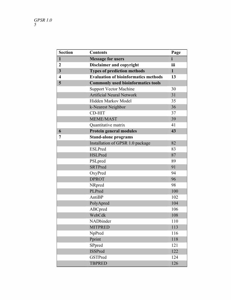
Section Contents Page1 Message for users i2 Disclaimer and copyright iii3 Types of prediction methods 14 Evaluation of bioinformatics methods 135 Commonly used bioinformatics tools

Support Vector Machine 30Artificial Neural Network 31Hidden Markov Model 35k-Nearest Neighbor 36CD-HIT 37MEME/MAST 39Quantitative matrix 41

6 Protein general modules 437 Stand-alone programs

Installation of GPSR 1.0 package 82ESLPred 83HSLPred 87PSLpred 89SRTPred 91OxyPred 94DPROT 96NRpred 98PLPred 100AntiBP 102PolyApred 104ABCpred 106WebCdk 108NADbinder 110MITPRED 113NpPred 116Pprint 118SPpred 121ISSPred 122GSTPred 124TBPRED 126

GPSR 1.0 6

PSEAPRED2 1288 List of contributors 130

GPSR 1.0 7

Types of Prediction

Methods

GPSR 1.0 8

GPSR 1.0 9

1. Prediction at Protein Level:These methods are developed to predict overall function of charactestics of proteins. Inthese methods we used complet protein as input. Following are few examples1.1 Subcellular level prediction:

The cellular localization of a protein is one of the most fundamental properties of anyprotein due to cellular division of labour. The correct prediction of subcellular locationcan be a major breakthrough for functional prediction, since to perform a function,protein must be located in their native location, such as nucleus or mitochondria oroutside the cell in case of secretory proteins. The native subcellular localization of aprotein is one of the indicators of protein function.Over the years numbers of methods have been developed for the prediction of subcellularlocalization in prokaryotes as well as eukaryotes. Existing subcellular localizationmethods can be divided into various categories:

1. Similarity search based techniques: query sequence is searched againstexperimentally annotated proteins.Limitation: fail to predict new/novel proteins, if query protein does not havesimilarity with known proteins.

2. Signal sequence based techniques: number of methods fall under this categoryin which leader sequence or sorting sequence present on protein itself is used forprediction. E.g. TargetP, PSORTb, SignalP

3. Sequence composition based techniques: number of methods has beendeveloped so far based on the sequence composition. e.g. SubLoc, NNPSL

4. Organism specific and location specific subcellular localization prediction:Organism specific approach is more useful than generalised approach.

MethodsSeveral computational tools for predicting the subcellular localization of a protein arepublicly available, a few of which are listed below:

Methods Techniques Used

PSLpred Composition based+SVM+PSI-BLAST

NRpred Composition based

GPCRpred Composition based

ESLpred SVM+Dipeptide Composition+PSI-BLAST

GPSR 1.0 10

SRTpred Composition based+physic-chemical properties+PSI-BLAST

Cytopred SVM+PSI-BLAST hybrid approach

PSEApred SVM

PFMpred SVM

HSLpred Composition based+SVM+PSI-BLAST

NNPSL Neural Network

RelevanceDetermining subcellular localization is important for understanding protein functionand is a critical step in genome annotation. Knowledge of the subcellular localizationof a protein can significantly improve target identification during the drug discoveryprocess. For example, secreted proteins and plasma membrane proteins are easilyaccessible by drug molecules due to their localization in the extracellular space or onthe cell surface.Subcellular localization prediction allows researchers to make inferences regarding aprotein's function, to annotate genomes, to design proteomics experimentsand—particularly in the case of bacterial pathogen proteins—to identify potentialdiagnostic, drug and vaccine targets.

1.2 Class level prediction:1.2.1 Classification of proteins

GPCRsclass: classification of amine type of G-protein-coupled receptors

1.2.2 Nucleotide binding protein prediction:Most of the functions of DNA/RNA are performed through interaction with proteins.Prediction of DNA/RNA binding Proteins can be categorised into 2 categories:Structure based methods: structure based methods can’t be used in high throughputannotation, as they require the structure of a protein for the predictionSequence based methods: Only couple of sequence based prediction methods havebeen developed so far. These methods are based on pseudo-amino acid composition,amino acid composition, composition of physico-chemical properties and SupportVector Machine (SVM).

METHODS:DISIS: predicts DNA binding sites directly from amino acid sequence

GPSR 1.0 11

DBS-Pred: predict DNA-binding proteins using amino acid composition

1.3 Family level predictionComputational prediction and classification of GPCRs can supply significantinformation for the development of novel drugs in pharmaceutical industry.

GPCRpred: An SVM Based Method for Prediction of families and subfamiliesof G-protein coupled receptorsGSTPred: prediction of GST proteinsGPCRsIdentifier: a corresponding stand-alone executable program for GPCRidentification and classification.

1.4 Structure class of proteinsProclass: predict the class of protein from its amino acid sequenceTBBpred: predicts the transmembrane Beta barrel regions in a given proteinsequence

2. Prediction at Residue level:2.1 Prediction of Nucleotide binding residues:Structural and physical properties of DNA provide important constraints on thebinding sites formed on surfaces of DNA-binding proteins. Characteristics of suchbinding sites may be used for predicting DNA-binding sites from the structural andeven sequence properties of unbound proteins. This approach has been successfullyimplemented for predicting the protein-protein interface. Here, this approach isadopted for predicting DNA-binding sites in DNA-binding proteins. First attempt touse sequence and evolutionary features to predict DNA-binding sites in proteins weremade by Ahmad et al. (2004) and Ahmad and Sarai (2005). Some methods usestructural information to predict DNA-binding sites and therefore require a 3-dimensional structure of the protein, while others use only sequence information anddo not require protein structure in order to make a prediction. Structure- andsequence-based prediction of DNA-binding residues in DNA-binding proteins can beperformed on several web servers listed below:

1. Pprint (Prediction of Protein RNA- Interaction): is a web-server for predictingRNA-binding residues of a protein. The prediction is done by SVM model trainedon PSSM profile generated by PSI-BLAST search of 'nr' protein database.

2.2 Post-translational modifications of proteinsISSPred: Intein Splice Site PredictionDictyOGlyc: O-(alpha)-GlcNAc glycosylation sites (trained on Dictyostelium

GPSR 1.0 12

discoideum proteins)NetAcet: N-terminal acetylation in eukaryotic proteinsNetCGlyc: C-mannosylation sites in mammalian proteinsNetCorona: Coronavirus 3C-like proteinase cleavage sites in proteinsNetNGlyc: N-linked glycosylation sites in human proteinsNetOGlyc: O-GalNAc (mucin type) glycosylation sites in mammalian proteinsNetPhos: Generic phosphorylation sites in eukaryotic proteinsNetPhosBac: Generic phosphorylation sites in bacterial proteinsProP: Arginine and lysine propeptide cleavage sites in eukaryotic protein

sequences

2.3 Secondary structure prediction:APSSP2: Advanced Protein Secondary Structure Prediction Server

2.4 Turn prediction:BhairPred: SVM based method for prediction of beta-hairpins in proteinsBTEVAL: Evaluation of beta turns prediction methodsBetaTPred: predicting ß-turns in a protein from the amino acid sequenceBetaTPred2: Prediction of ß-turns in proteins using neuralnetworks and multiple alignmentsBetaturns: Prediction of beta-turn typesAlphaPred: predicts the alpha turn residues in the given protein sequenceGammaPred: predicts the gamma turn residues in the given protein sequence

RELEVANCE:Useful application of DNA-binding residues prediction would be the identification ofproteins that bind to DNA. Recognition of probable binding sites both on the protein andthe DNA will go a long way in diagnosing the basis of these interactions. Their discoverycan help lead subsequent works such as site-directed mutagenesis and constrainedmacromolecular docking. Prediction of functional sites to act as filters in a predictivescheme for docking can be as effective as manually introducing biological constraints.

The identification of DNA-binding sites can also assist in prediction of DNA-bindingbehaviour of a protein. This is similar in spirit to other studies that assign functions to aprotein on the basis of functional sites discovered on its surface, such as protein-proteinand protein-DNA interaction sites.

3. Prediction at peptide/epitope level:The potential importance of epitope identification in developing vaccines against

GPSR 1.0 13

infectious, immune and other antigen-related diseases, epitopes are studied widely byresearchers in various fields, and a large expansion of databases, predictive methods andsoftware focussing on different types of epitopes has been witnessed. The averageimmunologists are overwhelmed with such a broad array of immunological analysis toolsthat are highly specific in use, not well understood or defined, tested on limited data andnot publicly accessibleEpitope prediction dates back to 1981 when the first B cell epitope prediction methodwas developed by Hopp and Woods. Since then many more methods have beendeveloped or adapted from other computational tools; for example B cell epitopeprediction and T cell epitope prediction. Despite the early start, however, predictionsystems for B cell epitopes are still in their infancy.

General epitope prediction methods

1. Sequence-based epitope predictionSequence-based method utilises the notion that sequence dictates structure andidentical structure in turn leads to identical functions. T cell epitopes have a commonsequence pattern or motif, as well as MHC allele specificity determining subpatterns.To make useful, informative epitope prediction, epitope physicochemical propertiesare also used, such as exposed surface, accessibility, flexibility, hydrophilicity,charge, number of proline residues, the proximity of the segment towards the C- or N-terminal of the protein, etc. Due to the enormous number of physicochemicalproperties that are associated with epitopes, simpler quantitative descriptors of aminoacid properties are sometimes used to simplify computation.Techniques, such as binding motifs, quantitative matrices (QM), virtual matrices,machine learning algorithms (ANN, HMM, SVM), evolutionary algorithms, linearprogramming, etc. are used to identify the binding peptide. They all have theirrelative advantages and disadvantages. For example, in a comparative study, Yu et al.suggested that motifs give the most accurate MHC-peptide binding predictions with alimited dataset, but as the data volume increases, machine learning predictionsbecome more reliable.

2. Structure-based epitope predictionThe structure-based prediction model bases on 3D protein structure to screenpotential binders. Structural similarity between query protein and template proteinsare used to predict epitopes of interest.

3. Hybrid prediction methods: combining sequential with structural analysisGiven the poor performance of epitope predictors based on sequence or structure

GPSR 1.0 14

analysis, it is clear that any single method cannot accurately predict epitopes.Consequently, some researchers turned to building predictive methods takingadvantage of both sequential and structural information. For example, a new methodwhich integrates 3D protein structure with physicochemical properties of amino acidsusing machine learning methods like Hidden Markov Model (HMM), supportingvector machine (SVM), ANN, etc. improved the prediction precision to a thoughsmall but significant degree. Like structural-based approach, its further developmentis hampered by the limited availability of 3D structure data of antigens and truenegative datasets, both to construct better predictors and evaluate the algorithms.There is also the possibility of false positives because different antibodies haveoverlapping binding sites.

METHODS1. ProPred: predicting binders of 51 HLA-DR (MHC class II of human) alleles.2. Propred1: binding peptides of MHC class I alleles. Matrix based methods3. nHLAPred: Promiscuous MHC class I restricted T cell epitopes: ANN, QM4. CTLPred: predicting cytotoxic T lymphocyte (CTL) epitopes in an antigenic

sequence: SVM, QM, ANN5. TAPPred: predicting TAP binding peptide in a protein6. BcePred: Prediction of linear B-cell epitopes, using physico-chemical

properties7. ABCPred: predict B cell epitope(s) in an antigen sequence, using artificial

neural network8. Pcleavage: SVM based method for Proteosome cleavage prediction9. MMBpred: predict mutated high affinity and promiscuous MHC class-I

binding peptides from protein sequence10. HLA-DR4Pred: an SVM and ANN based HLA-DRB1*0401(MHC class II

alleles) binding peptides prediction method

RELEVANCE:The implication of epitope prediction in both public health and basic scientific research isvast. It is applicable to all epitope-related research, such as discovery of peptidecandidate for subunit vaccines, autoimmune diseases study, allergy treatment, proteinstructural study, experiment design, etc. Developing epitope predictive methods andsoftware to identify and map potential epitopes from an antigen protein is vital to contestthe immune and infectious diseases. Drug development is the major financial drive forepitope prediction. Epitope-based vaccines have been shown to have promising resultsand confer protection to animal models in clinical trials, supporting the prophylactic,therapeutic and protective effects of these vaccines. The advantages of subunit vaccines

GPSR 1.0 15

over other types of vaccines are pronounced. Therefore, huge resources are beingchannelled into developing subunit vaccines against important, intractable diseases suchas cancer, HIV/AIDS, HCV and many other infectious, viral and immune diseases.However, despite its huge implications in public health, security and scientific arena,epitope prediction tools may be abused by terrorists to make biochemical weapons, andaccelerate pathogen evolution and mutation. Another concern is that the application ofepitope predictive software in discovering epitopes bias subsequent predictors, asresearchers would normally narrow peptide targets by predicting possible epitopes firstand then conduct experiments to discover epitopes, which in turn will be analysed todevelop other epitope predictive software.

4. Prediction based on signal sequences:Protein localization is important as protein function may be localized to specific areasinside the cell or within cellular organelles. These bioinformatics programs and databasescontain information and are able to predict where a protein may be localized based onsignal sequences or localization sequences contained within the protein. Methodsinvolving the recognition of N-terminal signal sequences; as the strong biologicalimplication because the signal sequence specifying the cellular location of a protein islocated at the N-terminus (Emanuelsson et al., 2000 and Reczko and Hatzigerrorgiou,2004). However, it is difficult to recognize underlying features from a highly divergedsignal sequence and to vectorize those features.

METHODS:

pTARGET: (Guda and Subramaniam, 2005) uses amino acid composition andlocalization-specific Pfam domains to assign a eukaryotic protein to one of ninelocalization sites.SecretomeP: (Bendtsen et al, 2004) predicts eukaryotic proteins which are secreted via anon-traditional secretory mechanism.SignalP: (Bendtsen et al, 2004) predicts traditional N-terminal signal peptides in bothprokaryotic and eukaryotic proteins.TargetP: (Emanuelsson et al, 2000) predicts the presence of signal peptides, chloroplasttransit peptides, and mitochondrial targeting peptides for plant proteins, and the presenceof signal peptides and mitochondrial targeting peptides for eukaryotic proteins.ChloroP: Chloroplast transit peptides and their cleavage sites in plant proteins

5. Prediction based on Motifs:The rapid increase in genomic information requires new techniques to infer proteinfunction and predict protein-protein interactions. Bioinformatics identifies modular

GPSR 1.0 16

signalling domains within protein sequences with a high degree of accuracy. In contrast,little success has been achieved in predicting short linear sequence motifs within proteinstargeted by these domains to form complex signalling networks. Predictions fromdatabase searches for proteins containing motifs matching two different domains in acommon signaling pathway provide a much higher success rate. This technologyfacilitates prediction of cell signalling networks within proteomes, and could aid in theidentification of drug targets for the treatment of human diseases.Techniques used for finding motifs in given protein sequences:

MEME: tool for discovering motifs in a group of related DNA or protein sequences.

Prosite: This program allows to scan a protein sequence (either from Swiss-Prot orTrEMBL or provided by the user) for the occurrence of patterns and profiles stored in thePROSITE database, or to search protein databases with a user-entered pattern.

PRINTS: is a compendium of protein fingerprints. A fingerprint is a group of conservedmotifs used to characterise a protein family; its diagnostic power is refined by iterativescanning of a SWISS-PROT/TrEMBL composite. Usually the motifs do not overlap, butare separated along a sequence, though they may be contiguous in 3D-space.

METHODS:

Pseapred: prediction of secretory proteins of P.falciparum method employs MASTtechnique along with PSI-BLAST and PSSM.

TBpred: prediction server that predicts four subcellular localization (cytoplasmic,integral membrane, secretory and membrane attached by lipid anchor) of mycobacterialproteins .It is SVM based method that exploits different features of protein such as aminoacid composition, dipeptide composition and position specific scoring matrix (PSSM).Along with SVM other techniques like profile HMM and MEME/MAST motif basedstudies were also applied. Moreover a hybrid approach combining the PSSM based SVMmodel and the MEME/MAST model has been incorporated.

6. Prediction based on Domains:Protein domain prediction is important for protein structure prediction, structuredetermination, function annotation, mutagenesis analysis and protein engineering.Protein domains are structural, functional and evolutionary units of proteins. Theprediction of domains from sequence information can improve tertiary structureprediction; enhance protein function annotation, aid structure determination and guide

GPSR 1.0 17

protein engineering and mutagenesis.The identification of domains within a protein sequence is an important precursor for arange of methods. Protein structural determination method such as X-ray crystallographyand NMR has size limitations which limit their use - they are often employed moresuccessfully when solving smaller domain units rather than whole chains.

METHODS:

MITPred: method for predicting the proteins which are destined to localize inmitochondria. In this method Domain search technique is also employed using myHMMER (hidden Markov Models based search) along with BLAST and SVM.

RELEVANCE:Domains provide one of the most valuable information for the prediction of proteinstructure, function, evolution and design. Accurate prediction of domain boundariesforms a basis of many types of protein research. New proteins such as chimeric proteinscan be created as they are composed of multifunctional domains (Suyama & Ohara,2003). The search method for templates used in comparative modeling can also beoptimized by the delineation of domain boundaries (Contreras-Moreira & Bates, 2002).As for threading methods, the domain boundary prediction can improve its performanceby enhancing the signal-to-noise ratio (Wheelan et al., 2000). Accurate identification ofdomain boundaries for homologous domains plays a key role for reliable multiplesequence alignment (Gracy & Argos, 1998).

7. Prediction based on Profiles: Classic profile-based prediction worked well for early single-issue, in-order executionprocessors, but fails to accurately predict the performance of modern processors. Themajor reason is that modern processors can issue and execute several instructions at thesame time, sometimes out of the original order and cross the boundary of basic blocks.Prosite is a method of determining what is the function of uncharacterized proteinstranslated from genomic or cDNA sequences. It consists of a database of biologicallysignificant sites and patterns formulated in such a way that with appropriatecomputational tools it can rapidly and reliably identify to which known family of protein(if any) the new sequence belongs.A profile, or weight matrix, is a table of position-specific amino acid weights and gapcosts. These numbers (also referred to as scores) are used to calculate a similarity scorefor any alignment between a profile and a sequence, or parts of a profile and a sequence.An alignment with a similarity score higher than or equal to a given cut-off value

GPSR 1.0 18

constitutes a motif occurrence. As with patterns, there may be several matches to a profilein one sequence, but multiple occurrences in the same sequences must be disjoint (non-overlapping) according to a specific definition included in the profile.

METHODS:

TBpred: prediction server that predicts four subcellular localization (cytoplasmic,integral membrane, secretory and membrane attached by lipid anchor) of mycobacterialproteins. It is SVM based method that exploits different features of protein such as aminoacid composition, dipeptide composition and position specific scoring matrix (PSSM).Along with SVM other techniques like profile HMM and MEME/MAST motif basedstudies were also applied. Moreover a hybrid approach combining the PSSM based SVMmodel and the MEME/MAST model has been incorporated.

PPrint: is a web-server for predicting RNA-binding residues of a protein. The predictionis done by SVM model trained on PSSM profile generated by PSI-BLAST search of 'nr'protein database.

PFMpred: Predicting mitochondrial proteins of P.falciparum

ESLPred2: Prediction of subcellular localization of eukaryotic proteins

GPSR 1.0 19

Evaluation ofBioinformatics

Methods

GPSR 1.0 20

Cross-Validation Technique

Cross-validation is a statistical method for validating a predictive model. Subsets of thedata are held out, to be used as validating sets, a model is fit to the remaining data (atraining set) and used to predict for the validation set. Averaging the quality of thepredictions across the validation sets yields an overall measure of prediction accuracy.In cross-validation, the original data set is partitioned into smaller data sets. The analysisis performed on a single subset, with the results validated against the remaining subsets.The subset used for the analysis is called the “training” set and the other subsets arecalled “validation” sets (or “testing” sets).

Jack Knife Test

Cross ValidationTechniques

Jack KnifeTest

Leave one out cross validation K-Fold Cross Validation

Monte CarloTest

Three wayssplit Test

DisjointSetsTest

BootStrapping

GPSR 1.0 21

Jackknifing, which is similar to bootstrapping, is used in statistical inferencing toestimate the bias and standard error in a statistic, when a random sample of observationsis used to calculate it. The basic idea behind the jackknife estimator lies in systematicallyrecomputing the statistic estimate leaving out one observation at a time from the sampleset. From this new set of "observations" for the statistic an estimate for the bias can becalculated and an estimate for the variance of the statistic.

K-fold Cross-validation- For each of K experiments, use K-1 folds for training and adifferent fold for Testing .This procedure is illustrated in the following figure for K=4

• Advantage of K-Fold Cross validation is that all the examples in the dataset areeventually used for both training and testing.

• Disadvantage of this method is that the training has to be completed k times,meaning it takes k times as much computation time

Leave-one Out Cross-validation- Leave-one-out is the degenerate case of K-Fold CrossValidation, where K is chosen as the total number of examples.• For a dataset with N examples, perform N experiments• For each experiment use N-1 examples for training and the remaining example for

testing.

GPSR 1.0 22

Advantage: Makes best use of the data Involves no random sub sampling

Disadvantage: Very computationally expensive and stratification is not possible.

Bootstrapping TechniqueBootstrapping technique is a statistical method for estimating the sampling distribution ofan estimator by sampling with replacement from the original sample, most often with thepurpose of deriving robust estimates of standard errors and confidence intervals of apopulation parameter like a mean, median, proportion, odds ratio, correlationcoefficient or regression coefficient. It is often used as a robust alternative to inferencebased on parametric assumptions when those assumptions are in doubt, or whereparametric inference is impossible or requires very complicated formulas for thecalculation of standard errors.Sample a dataset of n instances n times with replacement to form a new dataset of ninstances. Use this data as the training set. The remaining examples that were not selectedfor training are used for testing .Randomly select (with replacement) N examples and usethis set for training. The remaining examples that were not selected for training is usedfor testing .This value are likely to change from fold to fold.Repeat this process for a specified number of folds (K).

GPSR 1.0 23

Monte Carlo MethodMonte Carlo methods are a class of computational algorithms that rely on repeatedrandom sampling to compute their results. This method often used when simulatingphysical and mathematical systems. This can be loosely described as a statistical methodused in simulation (a method that utilizes sequences of random numbers as data) of data. Monte Carlo methods are used to solve various problems by generatingsuitable random numbers and observing that fraction of the numbers obeying someproperty or properties. The method is useful for obtaining numerical solutions toproblems which are too complicated to solve analytically.As this method is mainly depend upon random number. So, random number is uniqueevery time. For example a dataset of 200 sequences generate random number (24, 19, 74,38, 45, 38, 45, 38, 45, 38, 45) .Here the number 38 and 45 repeat many times. This willunnecessarily waste time and give bias model that is not accurate.

Advantage: As number of iteration is better will be the result. For example 10000iterations give more accurate result as compared to 100 iterations.

Disadvantage: Like any other statistical methods any bias in random number generatorwill affect the results.If the model develop during training is wrong, the result may be wrong.

Positive Data(N=100)

Negative Data(N=100)

Total Data (N=200)

Generate (X=10) random no. in ange 1-200 (eg- 5,7,28,3,55,57,62,67,89,9)

GPSR 1.0 24

Three Way Split Technique

Three Way Split Technique

If model selection and true error estimates are to be computed simultaneously, the dataneeds to be divided into three disjoint sets.Training set: A set of examples used for learning: to fit the parameters of the classifier.Validation set: A set of examples used to tune the parameters of a classifier.Test set: A set of examples used only to assess the performance of a fully-trainedclassifier.

NOTE: The tie between the bootstrap and Monte Carlo simulation of a statistic is obvious: Bothare based on repetitive sampling and then direct examination of the results. A big differencebetween the methods, however, is that bootstrapping uses the original, initial sample as thepopulation from which to resample, whereas Monte Carlo simulation is based on setting up a datageneration process (with known values of the parameters). Where Monte Carlo is used to test driveestimators, bootstrap methods can be used to estimate the variability of a statistic and the shape ofits sampling distribution.

Flow Chart shows the Stepwise procedure of Monte Carlomethod

Trainingset1 Test set1

Trainingset2

Trainingset3

Trainingset4

Validationset2

Validationset3

Validationset4

Test set2

Test set3

Test set4

Validationset1

Trai

nin

Model Errorrate

GPSR 1.0 25

Dis-Joint Test

Two sets are said to be disjoint if they have no element in common. eg- A={1, 2, 3} and

B={4, 5, 6} are disjoint sets. This definition can be extends to any collection of sets. A

collection of sets is pairwise disjoint or mutually disjoint. eg- Set A={1, 2}, Set B = {2,

3} and Set C= {3, 1} the intersection of the collection A, B and C is empty, so this is

mutually disjoint set but the collection is not pairwise disjoint. In fact, there are no two

disjoint sets in the collection.

Criteria using disjoint sets

Number of element/sequences in each set is at least 30.

Set must be pairwise disjoint set otherwise there is bias during training that will result

in over prediction.

It is important that the test set is not used in any way to create the classifier.

Flow Chart shows the Stepwise procedure of three way splittechnique

PROCEDURE OUTLINE:1. Divide the available data into training, validation and test set2. Select architecture and training parameters3. Train the model using the training set4. Evaluate the model using the validation set5. Repeat steps 2 through 4 using different architectures and training parameters6. Select the best model and train it using data from the training and validation sets7. Assess this final model using the test set

Procedure Outline:1. Make Positive and Negative datasets in two files. eg- N number sequences for positive

and N number for negative sequences.

2. Combine these two file in two a single file.eg- N+N=2N

3. Make X no. of sets that are pair wise disjoint set means not two sets have commonelement/sequence and also not a single element/sequence is repeated in a single set.

4. Make Training set and Test set like

5. Training Set Test Set

GPSR 1.0 26

Non-redundant Five-fold Cross-validationIdeally sequence in dataset should have minimum sequence similarity (e.g., less than30% in case of proteins) but it decrease size of dataset significantly. The performance ofSVM model directly proportional to size of dataset used for training. We can use non-redundant five-fold cross validation technique, where sequences in dataset were clusteredbased on sequence similarity. These clustered were divided into five sets; it means allsequences of a cluster were kept in one set. Thus no two sets have similar sequences; itmeans sequences in training and testing sets have no sequence similarity. We can makeclusters using Blastclust and CD-HIT even blastall may also use for this purpose. Byusing this technique we make non-redundant dataset without decreasing dataset size.

Measuring Performance

Measuring Performance

Classification Method Regression Method StatisticalMethod

GPSR 1.0 27

Actual

Positive Negative

Positive TP FP PPV

Negative FN TN NPVPre

dict

ed

Sensitivity Specificity

Threshold Dependent Parameters

Example: 203 people were examined for checking the probability of lung cancer

P Actual

Figure: Criteria of classification of a prediction into TP, TN, FPand FN

Threshold Dependent

1. Sensitivity

2. Specificity

3. Accuracy

4. PPV, NPV

5. MCC

1. ROC

2. AUC

3. Reliabilityindex

1. R, R2, Q2

2. MAE/AAE

3. RMSE

4. RMSECV

ThresholdIndependent

1. Z-test

2. P-test

3. t-test

GPSR 1.0 28

Positive(sick) Negative (Healthy)

Positive

(Sick) TP=2 FP=18

PPV

=2 / (2 + 18)

=10%

Negative

(Healthy) FN=1 TN=182

NPV

=182 / (1 + 182)

=99.5%

Sensitivity

=2/(2+1)

=66.67%

Specificity

=182/18+182

=91%

• True positive (TP) : Sick people correctly diagnosed as sick• False positive (FP) : Healthy people wrongly identified as sick• True negative (TN) : Healthy people correctly identified as healthy• False negative (FN) : Sick people wrongly identified as healthy

Sensitivity or percentage coverage of positive is the percentage of positive examplepredicted as positive.

100FN+TP

TP=Senstivity ×

A sensitivity of 100% means that the test recognizes all sick people as such. Thus in ahigh sensitivity test, a negative result is used to rule out the disease.Sensitivity alone does not tell us how well the test predicts other classes (that is, aboutthe negative cases). In the binary classification, as illustrated above, this is thecorresponding specificity test, or equivalently, the sensitivity for the other classes.

Specificity or percentage coverage of negative is the percentage of negative examplespredicted as negative.

100FP+TN

TN=Specifity ×

A specificity of 100% means that the test recognizes all healthy people as healthy. Thus apositive result in a high specificity test is used to confirm the disease. The maximum istrivially achieved by a test that claims everybody healthy regardless of the true condition.

GPSR 1.0 29

Therefore, the specificity alone does not tell us how well the test recognizes positivecases. We also need to know the senstivity of the test to the class, or equivalently, thespecificities to the other classes.

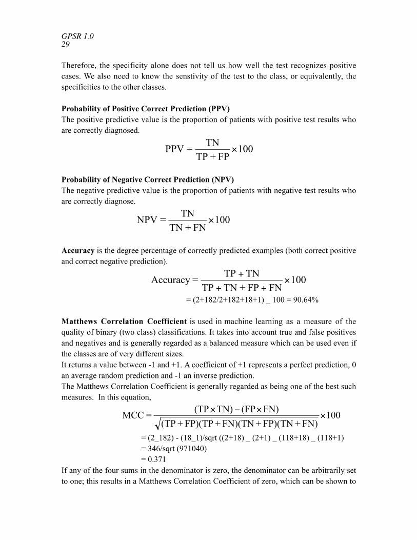
Probability of Positive Correct Prediction (PPV)The positive predictive value is the proportion of patients with positive test results whoare correctly diagnosed.

100FP+TP

TN=PPV ×

Probability of Negative Correct Prediction (NPV)The negative predictive value is the proportion of patients with negative test results whoare correctly diagnose.

100FN+TN

TN=NPV ×

Accuracy is the degree percentage of correctly predicted examples (both correct positiveand correct negative prediction).

100FN FP+TN TP

TN TP=Accuracy ×

+++

= (2+182/2+182+18+1) _ 100 = 90.64%

Matthews Correlation Coefficient is used in machine learning as a measure of thequality of binary (two class) classifications. It takes into account true and false positivesand negatives and is generally regarded as a balanced measure which can be used even ifthe classes are of very different sizes.It returns a value between -1 and +1. A coefficient of +1 represents a perfect prediction, 0an average random prediction and -1 an inverse prediction.The Matthews Correlation Coefficient is generally regarded as being one of the best suchmeasures. In this equation,

100FN)+FP)(TN+FN)(TN+FP)(TP+(TP

FN)(FPTN)(TP=MCC ×

×−×

= (2_182) - (18_1)/sqrt ((2+18) _ (2+1) _ (118+18) _ (118+1) = 346/sqrt (971040)

= 0.371If any of the four sums in the denominator is zero, the denominator can be arbitrarily setto one; this results in a Matthews Correlation Coefficient of zero, which can be shown to

GPSR 1.0 30

be the correct limiting value.

Threshold Independent ParameterReceiver operating characteristic (ROC) or simply ROC curve is a graphical plot ofthe sensitivity vs. (1- specificity) for a binary classifier system as its discriminationthreshold is varied. The ROC can also be represented equivalently by plotting the fractionof true positives (TPR = true positive rate) vs. the fraction of false positives (FPR = falsepositive rate) also known as a Relative Operating Characteristic curve, because it is acomparison of two operating characteristics (TPR & FPR) as the criterion changes.ROC analysis provides tools to select possibly optimal models and to discard suboptimalones independently from (and prior to specifying) the cost context or the classdistribution. ROC analysis is related in a direct and natural way to cost/benefit analysis ofdiagnostic decision making. ROC analysis has more recently been used in medicine,radiology, psychology, and other areas for many decades, and it has been introducedrelatively recently in other areas like machine learning and data mining.AUC: The area under the ROC curve, is called Area under the curve (AUC), or A'(pronounced "a-prime"). If AUC value is more than 0.5 then our model is working wellotherwise it’s a worse model.

Reliability IndexReliability index is a simple indication of level of certainty in the prediction. This RIcalculated by the following given equation-

RI is used in multiclass classification study. Assignment of RI to each sequence based

GPSR 1.0 31

upon the difference of highest and second highest score of various 1-vs-rest SVMs inmulti-class classification.

Regression Method

Regression/Real Value: We used machine learning techniques in regression/real-valueprediction. In this we predict real value as melting point, boiling point, IC50, Kd, EC50 etc.These are the parameter which gives explanation how good predicted values are good incompare to its real value. To access model performance and provide statisticallymeaningful data, we can calculate different statistical parameters. Here I am givingformulas using melting point (MP) as an example.

Actual MP ( )actMP P r e d i c t e d M P( )predMP

12.5 14.067.0 71.371.2 68.7115.9 121.032.7 29.845.7 49.379.8 76.8127.3 125.157.6 50.237.2 33.8

( )∑ actMP = 646.90 ( )∑ predMP = 640.0

( )∑2actMP = 53580.21 ( )∑

2predMP = 53169.64

predact MPMP∑ = 53297.66

Mean ( PM ): The arithmetic mean is the "standard" average, often simply called the"mean".

∑m

=im=

1

actMP1

MP

So here mean of actualMP = 12.5+67.0+71.2+115.9+32.7+45.7+79.8+127.3+57.6+37.2/10 = 646.90/10 = 64.69

Similarly MPpred = 14.0+71.3+68.7+……../10

= 640.00/10 = 64.0

GPSR 1.0 32

Pearson's correlation/Sample correlation (R): In general statistical usage, correlationrefers to the departure of two random variables from independence. R is the Pearson'scorrelation coefficient of actual and predicted value, this give idea about the performanceof machine learning techniques.

( ) ( ) ( ) ( )∑ ∑∑ ∑

∑ ∑ ∑−−

−

pred2pred2act2act

predact predact

MPMPMPMP

MPMPMPMP R

nn

n=

R = 53297.66 – 646.90*646.0/sqrt (53580.21 - 646.902)*(53169.64 – 646.002) = 11896.06/11968.56 = 0.994Where n is the size of test set, MPpred is the predicted melting point and MPact is the actualmelting points. Value of R always ranges from -1 to +1 negative. Negative value of Rshows that there is inverse relationship within actual and predicted value; while positivevalue of R show that here positive relationship within actual and predicted value. If R = 0then it’s totally random prediction.

Coefficient of determination (R2): Coefficient of determination is the statisticalparameter for proportion of variability in model.

( )

( )∑

∑

−

−−

n

=i

n

=i=R

1

2act

1

2predact

2

PMMP

MPMP1

Sum of square of errors (SSE) = ( )∑ −n

=i 1

2predact MPMP

Sum of square of total (SST) = ( )∑ −n

=i 1

2act PMMP

Where MPpred is the predicted melting point and MPact is the actual melting points PM isthe mean of MPact. R2 = 1 – (SSE/SST)

=1 – (154.53/11732.249) = 0.87The coefficient of determination is also the arithmetic average of all M folds run. Valueof R2 always ranges within 0 to 1. Its value gives idea how these actual values are relatedwith predicted value. Higher values of R2 show that here linear relationship within actualand predicted and lower value shows that non-linear relationshipQ2 is another very important statistical parameter for the determination of variability inmodel.

GPSR 1.0 33

( )

( )∑

∑

−

−−

n

=i

n

=i=Q

1

2

trainact

1

2predact

2

MPMP

MPMP1

∑m

=im=

1

acttrain MP

1MP

If value is more 0.5 then models performance is good.RMSE is the root mean squared error of the predictions calculated according

( )∑=

−n

in=

1

2predact MPMP1

RMSE

= sqrt (154.53/10) = 3.931Where n is the size of test set, MPact is the actual melting point and MPpred is thepredicted melting point by different machine learning techniques. Like mean absoluteerror it’s also give idea how our predicted melting point is for away from actual meltingpoints.MAE/AAE is mean of absolute errors within actual and predicted value

| |∑ −n

=in=

1

predact MPMP1

MAE

= 1/10* (| 12.5-14.0| + |67.0-71.3|+ …..) = 3.59Its gives idea how our predicted value are for away from experimentally calculatedmelting point. Where n is the size of test set, MPact is the actual melting point and MPpred

is the predicted melting point by different machine learning techniques.RMSECV is the aggregate root mean squared error of the cross-validation. For an M foldcross-validation, it is defined as

( )∑=

M

1

2RMSEM

1 RMSECV

i

=

Statistical Method

z-Test- The Z-test compares sample and population means to determine if there is asignificant difference.It requires a simple random sample from a population with a Normal distribution andwhere the mean is known.Calculation The z measure is calculated as:

Z = (x - m) / SE

GPSR 1.0 34

where x is the mean sample to be standardizedm is the populations mean, SE is the standard error of the mean.

where s is the population standard deviation, n is the sample sizeThe z value is then looked up in a z-table. A negative z value means it is below thepopulation mean (the sign is ignored in the lookup table).• The Z-test is typically with standardized tests, checking whether the scores from a

particular sample are within or outside the standard test performance.• The z value indicates the number of standard deviation units of the sample from the

population mean.Note: z-test is not the same as the z-score, although they are closely related.

t-Test- The t-test assesses whether the means of two groups are statistically differentfrom each other. This analysis is appropriate whenever you want to compare the means oftwo groups.

In the formula of t-test numerator is difference between the means and denominator isstandard error of the difference between mean ,which is calculated by the variances foreach group and divide it by the number of people in that group. We add these two valuesand then take their square root.

The t-value will be positive if the first mean is larger than the second and negative if it issmaller. Once you compute the t-value you have to look it up in a table of significance totest whether the ratio is large enough to say that the difference between the groups is notlikely to have been a chance finding. To test the significance, you need to set a risk level(called the alpha level).p-Test: Hypothesis Tests About a ProportionIn p-test we would like to test the following three null hypotheses about a population

SE = s / sqrt(n)

GPSR 1.0 35

proportion p1. Ho: p <= P2. Ho: p >= P3. Ho: p = P

We can test each claim simultaneously with a sample proportion m / n, where m is thenumber of favorable (or "Yes") responses and n is the random sample size.If m / n are too large, then we must reject the first null hypothesis Ho: p <= P.If m / n are too small, then we reject the second null hypothesis. Ho: p >= PIf m / n are either too large or too small, then we reject the third null hypothesis. Ho: p =P

Once again, we conduct the tests with the use of the test statistic. If the population isconsidered "large," then we define the test statistic byIf the population is of a smaller, finite size N (so that the sample size n is more than 5%of the entire population), then we define the test statistic by

x = (m / n - P) / Sqrt[P(1 - P) / n].

x = (m / n - P) / [ Sqrt[ P(1 - P) / n] Sqrt[ (N - n) / (N - 1) ] ]

GPSR 1.0 36

Commonly used

Bioinformatics Tools

This chapter describes commonly used computational techniques like machine learning.The aim of this chapter is not to describe theory of these methods. Instead we havedescribes how to use these programs. We have describes these methods in short and

GPSR 1.0 37

simple words, so begineers may use these tools. The detail description of these programsis available from their manual or web site. Following are commonly used tools,particularly our group is using them to build new tools.

Support Vector Machine: How to use SVMlight

SVM is frequently used in bioinformatics for classifying proteins, predicting structures,epitop prediction etc. One of the major advantages of SVM over other machine learningtechniques is that it can be trained on small data set with minimum over-optimization.SVMlight is an implementation of Support vector Machines (SVMs) in C. SVMlight is animplementation of Vapnik’s Support Vector Machine for the problem of patternrecognition, for the problem of regression, and for the problem of learning a rankingfunction. The algorithm has scalable memory requirements and can handle problems withmany thousand of support vectors efficiently. The software also provides methods forassessing the generalization performance efficiently. It includes two efficient estimationmethods for both error rate and precision/recall.

How to use

SVMlight consists of a learning module (svm_learn) and a classification module(svm_classify). The classification module can be used to apply the learned model to newexamples. See also the examples below for how to use svm_learn and svm_classify.

Run the svm_learn program with different parameters for better optimization

svm_learn [options] example_file model_file svm_learn program build a model amd these model further use with svm_classify

program.

1. By the use of svm_classify we can predict the class of unknown protein, whetherit’s belongs to positive type or negative type.

svm_classify [options] example_file model_file output_file

svm_learn is called with the following parameters:

svm_learn [options] example_file model_file

GPSR 1.0 38

SVM input (for Positive sequence) SVM input (for Negative sequence)

Artificial Neural Network: How to use the SNNSfor implementing ANN

ANN is powerful machine learning techniques, commonly used for solving classificationproblem. They are capable to handle large datasets and non-linear proroblems efficiently.SNNS (Stuttgart Neural Network Simulator) is a software simulator for neural networkson Unix workstations developed at the Institute for Parallel and Distributed HighPerformance Systems (IPVR) at the University of Stuttgart. The goal of the SNNS projectis to create an efficient and flexible simulation environment for research on and

Create Positive Dataset(e.g. FASTA sequences)

Create Negative Dataset (e.g. FASTA sequences)

Now select the best distinguishable featuresfrom both types of datasets (for example herewe use amino acid composition)

SVM input for protein sequence:ACDEFGHIKLMNPQRSTWYA

+1 1:10 2:5 3:5 4:5 5:5 6:5 7:5 8:5 9:5 10:5 11:512:5 13:5 14:5 15:5 16:5 17:5 18:0 19:5 20:5

-1 1:10 2:5 3:5 4:5 5:5 6:5 7:5 8:5 9:5 10:5 11:512:5 13:5 14:5 15:5 16:5 17:5 18:0 19:5 20:5

GPSR 1.0 39

application of neural nets. One of the challenges is to implement SNNS, here we havegiven an example

Input file in fasta formatTotal number of sequence in this file is 78, only 10 are diplayedAn example of sequences in fasta format,

>Lec_protein1ADSGADSGFADSGDAGSFDAGDSGFADSGFADSGDAGSDAGDSGAD>Lec_protein2ASKDNAKSNDKJASNDKJANSKDNASKMDKMASNKDNASKJNDKAL>Lec_protein3XLKAMSLKXMALKSMXLKASMXLKASMXLMASLXMALSXMLAKS>Lec_protein4LJDLKAJSLKDJASLKJDLASJDLAJSLDJASLDLAJSLDKJALSJDLKAJS>Lec_protein5JRTLKERJLKTJELRJTLKERJTLKJERLKJTLKERJTLKJERLKTJERLKJT>Lec_protein6DLJASLKJDLASJDLKJASLDKJASLDJLASKJDLKJASLDJASLKJDALSK>Lec_protein7LASJDLAJSLDJASLJDALSJDLAJSLDJASLJDLASJDLKJASLDJALSJDLK>Lec_protein8ENRWMENRMWNERNWERNWERMWEMNRWENRMWENRNWMENRM>Lec_protein9NWEMWMENQNEQNEQMNEQMNWMENQWNEQNWEQMWNEMQWN>Lec_protein10LKASLKDJASJDLKAJSLDJASLJDLKASJASLJDALKSDLKJALDLKASJDL

Input file in SNNS formatIn order to generate fixed length pattern from variable length of sequence, we computeamino acid composition. Following is example input SNNS file generated for thesesequences where composition is feature. Following is descriptrion

Note that the first 7 lines of the input file. First two lines , followed by to blank line thenthe number of patterens (78 in this case, since total seqience is 78), number of input units(20 in this case, calculating the amino acid composition) and the out puts (1, one value)SNNS pattern definition files V4.2

Generated at Sat Aug 27 16:40:25 2005

GPSR 1.0 40

No. of patterns: 78No. of input units: 20No. of output units: 1

# Input pattern 1:0.1 0 0.2 0.2 0 0.1 0 0 0 0 0 0.1 0 0.3 0 0 0 0 0 0# Output pattern 1:1# Input pattern 2:0.1 0 0 0.5 0 0 0 0 0.1 0.1 0 0 0 0 0.1 0 0 0.1 0 0# Output pattern 2:1

Output file of SNNSThe out put file of the SNNS is shown. The result shows the summary of information.SNNS result file V1.4-3DGenerated at Tue Aug 30 08:58:52 2005

No. of patterns : 26No. of input units: 20No. of output units: 1Startpattern : 1Endpattern : 26Input patterns includedTeaching output included#1.10.1 0 0.1 0 0 0 0 0.1 0.1 0.20 0 0 0 0 0.1 0.1 0 0 0.210.64832#2.10 0 0.1 0.1 0.3 0.1 0 0 0 00 0 0.2 0.1 0 0 0.1 0 0 010.6276

The outputs of the SNNS are process at different threshold (0.1 to 1), and parameters like

Out put of SNNS

GPSR 1.0 41

sensitivity, specificity, and accuracy are calculated. The Artificial neural network tries toclassify positive from negative examples. For example here we take an example of IgEepitopes and non epitopes. We need a data set of IgE epitope (positive set) and negativeset (non epitopes). The Netwok will classify this training set, it will be validated by oneset (to stop over fitting) and then tested by the left out testing set. Each set contains equalnumber of sequence. In five fold cross validation it looks like this,

Training set Validation set Testing set

set 1,2,3 set 4 set 5

set 1,4,5 set 3 set 4

set 1,4,5 set 2 set 3

set 3,4,5 set 1 set 2

set 2,3,4 set 5 set 1

Processing of output dataThe out put data are processed and interpreted, as shown (Thres=Threshold;Sen=Sensitivity; Spe= Specificity; Acc=Accuracy; PPV=positive prediction value)Thres Sen Spe Acc PPV1.0000 0.0000 0.0000 0.0000 0.00000.9000 0.0214 0.9929 0.5071 0.75000.8000 0.1429 0.9857 0.5643 0.90910.7000 0.2571 0.9571 0.6071 0.85710.6000 0.5143 0.8357 0.6750 0.75790.5000 0.7214 0.7214 0.7214 0.72140.4500 0.8071 0.6000 0.7036 0.66860.4000 0.8571 0.4714 0.6643 0.61860.3000 0.9571 0.3286 0.6429 0.58770.2000 1.0000 0.1000 0.5500 0.52630.1000 000 0.0071 0.5036 0.5018

GPSR 1.0 42

HMMER: Bio-sequences analysis using profilehidden markov models

Introduction

HMMER is a freely distributable implementation of profile HMM software for proteinsequence analysis written by Sean Eddy. It is used for sensitive database search usingmultiple sequence alignments (profile-HMMs) as queries. The profile-HMMs are basedon the work of Krogh and colleagues. Basically, we give HMMER a multiple sequencealignment as input; it builds a statistical model called a "hidden Markov model" whichyou can then use as a query into a sequence database to find (and/or align) additionalhomologues of the sequence family. HMMER is a console utility ported to every majoroperating system including different versions of Linux, Windows and Mac OS.

HMMER generally contain following programs ---hmmalign Align sequences to an existing model.hmmbuild Build a model from a multiple sequence alignment.hmmcalibrate

Takes an HMM and empirically determines parameters that are used to makesearches more sensitive, by calculating more accurate expectation valuescores (E-values).

hmmconvertConvert a model file into different formats, including a compact HMMER 2binary format, and ``best effort'' emulation of GCG profiles.

hmmemit Emit sequences probabilistically from a profile HMM.hmmfetch Get a single model from an HMM database.hmmindex Index an HMM database.hmmpfam Search an HMM database for matches to a query sequence.hmmsearch Search a sequence database for matches to an HMM.

GPSR 1.0 43

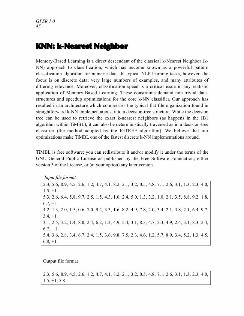
KNN: k-Nearest Neighbor

Memory-Based Learning is a direct descendant of the classical k-Nearest Neighbor (k-NN) approach to classification, which has become known as a powerful patternclassification algorithm for numeric data. In typical NLP learning tasks, however, thefocus is on discrete data, very large numbers of examples, and many attributes ofdiffering relevance. Moreover, classification speed is a critical issue in any realisticapplication of Memory-Based Learning. These constraints demand non-trivial data-structures and speedup optimizations for the core k-NN classifier. Our approach hasresulted in an architecture which compresses the typical flat file organization found instraightforward k-NN implementations, into a decision-tree structure. While the decisiontree can be used to retrieve the exact k-nearest neighbors (as happens in the IB1algorithm within TiMBL), it can also be deterministically traversed as in a decision-treeclassifier (the method adopted by the IGTREE algorithm). We believe that ouroptimizations make TiMBL one of the fastest discrete k-NN implementations around.

TiMBL is free software; you can redistribute it and/or modify it under the terms of theGNU General Public License as published by the Free Software Foundation; eitherversion 3 of the License, or (at your option) any later version.

Input file format2.3, 5.6, 8.9, 4.5, 2.6, 1.2, 4.7, 4.1, 8.2, 2.1, 3.2, 0.5, 4.8, 7.1, 2.6, 3.1, 1.3, 2.3, 4.0,1.5, +15.3, 2.6, 6.4, 5.8, 9.7, 2.5, 1.5, 4.3, 1.0, 2.4, 5.0, 1.3, 3.2, 1.0, 2.1, 3.5, 8.8, 9.2, 1.8,6.7, –14.2, 1.3, 2.0, 1.5, 0.6, 7.0, 9.4, 3.3, 1.6, 8.2, 4.9, 7.8, 2.0, 3.4, 2.1, 3.8, 2.1, 6.4, 9.7,3.4, +13.1, 2.5, 3.2, 1.4, 8.0, 2.4, 6.2, 1.3, 4.9, 5.4, 3.1, 8.3, 4.7, 2.3, 4.9, 2.4, 3.1, 8.3, 2.4,6.7, –15.4, 3.6, 2.8, 3.4, 6.7, 2.4, 1.5, 3.6, 9.8, 7.5, 2.3, 4.6, 1.2, 5.7, 8.9, 3.4, 5.2, 1.3, 4.5,6.8, +1

Output file format

2.3, 5.6, 8.9, 4.5, 2.6, 1.2, 4.7, 4.1, 8.2, 2.1, 3.2, 0.5, 4.8, 7.1, 2.6, 3.1, 1.3, 2.3, 4.0,1.5, +1, 5.8

GPSR 1.0 44

5.3, 2.6, 6.4, 5.8, 9.7, 2.5, 1.5, 4.3, 1.0, 2.4, 5.0, 1.3, 3.2, 1.0, 2.1, 3.5, 8.8, 9.2, 1.8,6.7, –1, 6.44.2, 1.3, 2.0, 1.5, 0.6, 7.0, 9.4, 3.3, 1.6, 8.2, 4.9, 7.8, 2.0, 3.4, 2.1, 3.8, 2.1, 6.4, 9.7,3.4, +1, 4.33.1, 2.5, 3.2, 1.4, 8.0, 2.4, 6.2, 1.3, 4.9, 5.4, 3.1, 8.3, 4.7, 2.3, 4.9, 2.4, 3.1, 8.3, 2.4,6.7, –1, 6.1

5.4, 3.6, 2.8, 3.4, 6.7, 2.4, 1.5, 3.6, 9.8, 7.5, 2.3, 4.6, 1.2, 5.7, 8.9, 3.4, 5.2, 1.3, 4.5,6.8, +1, 7.0

Class predicted value

This predicted values use in calculating TP, TN, FP and FN parameters.

TP : True Positive TN : True Negative FP : False Positive FN : FalseNegative

CD-HIT

1. CD-HIT: clustering and comparing large sets of sequences

Introduction

Cd-hit is a fast program for clustering and comparing large sets of protein or nucleotidesequences. The main advantage of this program is its ultra-fast speed. It can be hundredsof times faster than other clustering programs, for example, BLASTCLUST. Therefore itcan handle very large databases, like NR. Current CD-HIT package can perform variousjobs like clustering a protein database, clustering a DNA/RNA database, comparing twodatabases (protein or DNA/RNA), generating protein families, and many others.

CD-HIT clusters proteins into clusters that meet a user-defined similarity threshold,usually a sequence identity. Each cluster has one representative sequence. The input is aprotein dataset in fasta format and the output are two files: a fasta file of representativesequences and a text file of list of clusters.

Basic command:cd-hit -i nr -o nr100 -c 1.00 -n 5 -M 2000

GPSR 1.0 45

cd-hit -i db -o db90 -c 0.9 -n 5, wheredb is the filename of input,db90 is output,0.9, means 90% identity, is the clustering threshold5 is the size of word

Choose of word size:-n 5 for thresholds 0.7 ~ 1.0-n 4 for thresholds 0.6 ~ 0.7-n 3 for thresholds 0.5 ~ 0.6-n 2 for thresholds 0.4 ~ 0.5

CD-HIT-2D

CD-HIT-2D compares 2 protein datasets (db1, db2). It identifies the sequences in db2that are similar to db1 at a certain threshold. The input are two protein datasets (db1, db2)in fasta format and the output are two files: a fasta file of proteins in db2 that are notsimilar to db1 and a text file that lists similar sequences between db1 & db2.

Basic command:cd-hit-2d -i db1 -i2 db2 -o db2novel -c 0.9 -n 5, wheredb1 & db2 are inputs,db2novel is output,0.9, means 90% identity, is the comparing threshold5 is the size of wordPlease note that by default, I only list matches where sequences in db2 are not longer thansequences in db1. You may use options -S2 or -s2 to overwrite this default. You can alsorun command:cd-hit-2d -i db2 -i2 db1 -o db1novel -c 0.9 -n 5Choose of word size (same as cd-hit):-n 5 for thresholds 0.7 ~ 1.0-n 4 for thresholds 0.6 ~ 0.7-n 3 for thresholds 0.5 ~ 0.6-n 2 for thresholds 0.4 ~ 0.5

GPSR 1.0 46

MEME/MAST

MEME: MEME is a tool for discovering motifs in a group of related DNA or proteinsequences.

The MEME Suite software is available for FREE interactive use via the web or you candownload it on your local system from http://meme.nbcr.net/meme4_1/meme-download.html web link.

MEME takes as input a group of DNA or protein sequences and outputs as many motifsas requested. MEME uses statistical modeling techniques to automatically choose thebest width, number of occurrences, and description for each motif.

Program Execution:

meme meme_input_file (options) > meme_output_file

NUMBER OF MOTIFS-nmotifs <n> The number of *different* motifs to search for. MEME will search forand output <n> motifs. Default: 1

GPSR 1.0 47

-evt <p> Quit looking for motifs if E-value exceeds <p>.Default: infinite (so by defaultMEME never quits before -nmotifs <n> have been found.)

NUMBER OF MOTIF OCCURENCES-nsites <n>-minsites <n>-maxsites <n> the (expected) number of occurrences of each motif. If -nsites is given,only that number of occurrences is tried. Otherwise, numbers of occurrences between-minsites and -maxsites are tried as initial guesses for the number of motif occurrences.These switches are ignored if mod = oops.Default: -minsites sqrt (number sequences)-wnsites <n> the weight on the prior on nsites. This controls how strong the bias towardsmotifs with exactly nsites sites (or between minsites and maxsites sites) is. It is a numberin the range [0..1). The larger it is, the stronger the bias towards motifs with exactlynsites occurrences is. Default: 0.8

MOTIF WIDTH-w <n>-minw <n>-maxw <n>

The width of the motif(s) to search for. If -w is given, only that width is tried. Otherwise,widths between -minw and -maxw are tried. Default: -minw 8, -maxw 50 (defined inuser.h)

Note: If <n> is less than the length of the shortest sequence in the dataset, <n> is reset byMEME to that value.

MAST: MAST is a tool for searching biological sequence databases for sequencesthat contain one or more of a group of known motifs.

MAST takes as input a MEME output file containing the descriptions of one or moremotifs and searches a sequence database that you select for sequences that match themotifs

mast <meme_output_file> [-d <database>] [optional arguments ...]

<mfile> file containing motifs to use (meme_output_file)

GPSR 1.0 48

-d database to search with motifs

Quantitative matrix

The contribution of each residue (amino acid) for each position in a polypeptide chaincan be calculated with the use of Quantitative matrix. The QM is basically a propensity ofeach residue at a particular position. There are a number of equations, which can be usedfor matrix generation. The higher positive score of a residue at a given position meansthis residue is highly preferred at that position. The higher negative score means thatresidue is not preferred in peptides at that position. One of the major advantages of QM isthat the effect of each residue on specific activity of a peptide can be easily estimated.

Quantitative Matrix: These quantitative based methods consider the contribution ofeach residue at each position in peptide instead of anchor positions/residues. Quantitativematrices provide a linear model with easy to implement capabilities. Another advantageof using the matrix approach is that it covers a wider range of peptides with bindingpotential and it gives a quantitative score to each peptide. Their predictive accuracies areconsiderable.

Equation for Matrix Generation: There are a number of equations which can be usedfor matrix generation.

A few of which are as follows

Q (i,r) = P(i,r) – N(i,r) (1)

P (i,r) = E i,r / NP i,r (2)

N (i,r) = A i,r / NN i,r (3)

Where, Q(i,r) is the weight of any residue r at position 'i' in the matrix. 'r' can be anynatural amino acid and the value of 'i' can vary from 1 to 15. P(i,r) and N(i,r) is theprobability of residue 'r' at position 'i' in positive and negative peptides respectively. E i,rand A i,r is number residue 'r' at position 'i' in positive and negative peptidesrespectively, and NP i,r is the number of positive peptides and NN i,r is the number ofnegative peptides having residue 'r' at position 'i'.

GPSR 1.0 49

Example:

Generation of Quantitative matrices: The quantitative matrices consist of a tablehaving the sequence weight

Frequencies of each of the 21 amino acids (including "X") at each position in the datasetof MHC binders divided by the corresponding expected frequency of that amino acid inthe non-binders dataset. The MHC binder’s datasets for each MHC allele are generatedby obtaining MHC binders of 9 amino acids from MHCBN database. The equal numberof the non-binders is also obtained from the same database (if available) otherwise the 9-mer peptides are randomly chosen from the SWISS-PROT database. The quantitativematrices are addition matrices where the score of a peptide is calculated by summing upthe scores of each residue at specific position along peptide sequence. For example, thescore of peptide "ILKEPVHGV" is calculated as follows.

Score= I(1)+L(2)+K(3)+E(4)+P(5)+V(6)+H(7)+G(8)+V(9)

The peptides with score more than the cutoff score at a particular threshold are predictedas MHC binders. A fewmatrices are also obtained from literature (BIMAS andProPred1).These matrices are mostly multiplication matrices. The score of the peptide iscalculated as follows: e.g. "ILKEPVHGV"

Peptide score=I(1)*L(2)*K(3)*E(4)*P(5)*V(6)*H(7)*G(8)*V(9)

GPSR 1.0 50

Protein GeneralModules

GPSR 1.0 51

In this chapter we have described the small programs developed at our group; theseprograms can be used as building block to develop complex prediction modules. Thequestion arises how it is different then existing software libraries or modules likeBioPERL. InBioPER or similar packages one need to have knowledge of computerprogramming in order to uses these modules/subroutines. In GPSR package we havedeveloped small programs, which can be run by any person have little knowledge ofcomputers. Following are important programs included in this package.

Program Purpose fasta2sfasta Convert fasta format to single fasta format pro2aac To calculate amino acid composition of protein pro2aac_nt To calculate amino acid composition of N-terminal (nt) residues of a

protein

pro2aac_ct To calculate amino acid compositionof C-terminal (ct) residues of a protein

pro2aac_rest.pl To calculate amino acid composition of aprotein after removing N-, and C-terminal residues

pro2aac_split To calculate split amino acid composition (SSAC) of aprotein

pro2dpc To calculate dipeptide composition of protein pro2dpc_nt To calculate dipeptide composition of N-terminal (nt)

residues of a protein pro2dpc_ct To calculate dipeptide composition of C-terminal (ct)

residues of a protein pro2tpc To calculate tripeptide composition of protein add_cols To add columns of two files

col2svm To generating SVM_light input format col_mult To multiplying each column of input file with a number col_mult_sel To multiplying selective columns with a number perl col_rem To remove selective columns from a file col_ext To extract selective columns from a file

GPSR 1.0 52

col_corr To compute correlation co-efficient between two column

col_avg To calculate average column of two files seq2pssm_imp To calculate PSSM matrix in column format without any

normalization pssm_n1 To normalize pssm profile based on 1/(1+e-x) formula pssm_n2 To normalize pssm profile based on (numb -min)/(max -

min) formula pssm_n3 To normalize pssm profile based on (numb -

min)*100/(max -min) formula pssm_n4 To normalize pssm profile based on 1/(1+e-(x/100)

formula pssm_comp To compute PSSM composition (400 points) col_sig Significance of columns in two column files pssm2pat To generate patterns of given size from PSSM matrix pssm_smooth To designed smooth pssm profile for plot seq2motif To create motifs by sliding window of user defined length

with option of adding terminal X motif2bin To make binary input from the multifasta motif file blast_similarity To perform blast

GPSR 1.0 53

Title Description

Fasta formatfasta2sfasta (Convert fasta format to single fasta format) (Pearon format) is used to represent peptide sequences or nucleic acidsequences using single-letter codes. It begins with a single-line description,followed by lines of sequence data. The description line is distinguished fromthe sequence data by a greater-than (">") symbol.

Single fastaformat

Our programs use input sequence in single fasta format. Therefore, fasta fileshould first convert into single fasta format. In the single fasta format thedescription and sequence data merged into single line. Two hash marks (##)were present to distinguish description and sequence data.

Usage fasta2sfasta –i seq.fa -o seq.sfa

-i Input file name having sequence in fasta format

-o Output file name that gives sequence in single fasta format

seq.fa >seq_1MRNRGFGRRELLVAMAMLVSVTGCARHASGARPASTTLPAGADLADRFAELERRYDARLGVYVPATGTTAAIE>seq_2ACGRGFGVKLACNMNNACRTYFSDVAMAMLVSVTGCARHASGARPASTTLPAGADLADIEYRADERFAFCSTF

seq.sfa >seq_1##MRNRGFGRRELLVAMAMLVSVTGCARHASGARPASTTLPAGADLADRFAELERRYDARLGVYVPATGTTAAIE>seq_2##ACGRGFGVKLACNMNNACRTYFSDVAMAMLVSVTGCARHASGARPASTTLPAGADLADIEYRADERFAFCSTF

GPSR 1.0 54

Title Description

pro2aac (To calculate amino acid composition of protein)The amino acid composition in a protein is simply the percentage of thedifferent amino acids represented in a particular protein. The aim of calculatingthe composition of proteins is to transform the variable length of proteinsequences to fixed length feature vectors. This is an important and most crucialstep during classification of proteins using machine-learning techniquesbecause they require fixed length patterns. In addition the conversion of aprotein sequence to a vector of 20 dimensions using amino acid compositionwill encapsulate the properties of the protein into the vector.

The composition of all 20 natural amino acids were calculated by using thefollowing equation

Total number of amino acid i x 100Composition of amino acid i =

Total number of all amino acids in protein

Where i can be any amino acid

Usage pro2aac -i seq.sfa -o seq.out-i Input file name contains single fasta format-o Output file name gives amino acid compositionseq.sfa >seq_1##MRNRGFGRRELLVAMAMLVSVTGCARHASGARPASTTLPAGADLADRFAEL

ERRYDARLGVYVPATGTTAAIE>seq_2##ACGRGFGVKLACNMNNACRTYFSDVAMAMLVSVTGCARHASGARPASTTLPAGADLADIEYRADERFAFCSTF

seq.out # Amino Acid Composition of proteins# A , C , D , E , F , G , H , I , K , L , M , N , P , Q , R , S , T , V , W , Y,19.18, 1.37, 4.11, 5.48, 2.74, 9.59, 1.37, 1.37, 0.00, 9.59, 4.11, 1.37, ...... 2.74,19.18, 6.85, 5.48, 2.74, 6.85, 8.22, 1.37, 1.37, 1.37, 5.48, 4.11, 4.11, ...... 2.74,

Vector 20 dimension (i.e 20 types of amino acid composition is generated)

GPSR 1.0 55

Title Description

pro2aac_nt (To calculate amino acid composition of N-terminal (nt) residues of aprotein)It is well known that some proteins having N-terminal signal sequence which isresponsible to transport whole protein into their specific subcellular compartmentlike, lysosome, endoplasmic reticulum, mitochondria, and chloroplast. Evidencesindicate that divergent N-terminal sequences also do influence catalytic behavior,protein-protein interactions, and intracellular distributions of enzymes. Report showsthat N-terminal signal sequence can vary from 13 to 36 amino acid residues in lengthand having all the information needed to localize into specific location. Therefore,N-terminal information could be exploited by using amino acid composition featureto predict subcellular protein. For example:

N 5 nt C

Usage pro2aac_nt -i seq.sfa -o seq.out -n 5

-i Input file name

-o Output file name

-n Number of residues to calculate composition from N-terminal

seq.sfa >seq_1##MRNRGFGRRELLVAMAMLVSVTGCARHASGARPASTTLPAGADLADRFAELERRYDARLGVYVPATGTTAAIE>seq_2##ACGRGFGVKLACNMNNACRTYFSDVAMAMLVSVTGCARHASGARPASTTLPAGADLADIEYRADERFAFCSTF

Seq.out # Amino Acid Composition of 5 n-terminal residues of proteins# A , C , D , E , F , G , H , I , K , L , M , N , P , Q , R , S , T , V , W , Y, 0.00, 0.00, 0.00, 0.00, 0.00, 20.00, 0.00, 0.00, 0.00, 0.00, 20.00 ..... 0.00,20.00, 20.00, 0.00, 0.00, 0.00, 40.00, 0.00, 0.00, 0.00, 0.00, ..... 0.00,

Vector 20 dimension

GPSR 1.0 56

Title Description

pro2aac_ct (To calculate amino acid composition of C-terminal (ct) residues of aprotein)While the N-terminus of a protein often contains targeting signals, the C-terminuscan contain retention signals for protein sorting. The most common ER retentionsignal is the amino acid sequence -KDEL (or -HDEL) at the C-terminus, whichkeeps the protein in the endoplasmic reticulum and prevents it from entering thesecretory pathway. The C-terminus of proteins can be modified post-translationally,most commonly by the addition of a lipid anchor to the C-terminus that allows theprotein to be inserted into a membrane without having a transmembrane domain.The c-terminal domain of RNA polymerase II typically consists of up to 52 repeatsof the sequence Tyr-Ser-Pro-Thr-Ser-Pro-Ser. Other proteins often bind the C-terminal domain of RNA polymerase in order to activate polymerase activity. It isthe protein domain, which is involved in the initiation of DNA transcription, thecapping of the RNA transcript, and attachment to the spliceosome for RNAsplicing. Therefore the information at C-terminal in could be utilized using aminoacid composition feature to predict different classes of proteins. For example:

N 5nt C

Usage pro2aac_ct -i seq.sfa -o seq.out -n 5

-i Input file name

-o Output file name

-n Number of residues to calculate composition from C-terminal

seq.sfa >seq_1##MRNRGFGRRELLVAMAMLVSVTGCARHASGARPASTTLPAGADLADRFAELERRYDARLGVYVPATGTTAAIE>seq_2##ACGRGFGVKLACNMNNACRTYFSDVAMAMLVSVTGCARHASGARPASTTLPAGADLADIEYRADERFAFCSTF

seq.out # Amino Acid Composition of 5 c-terminal residues of proteins# A , C , D , E , F , G , H , I , K , L , M , N , P , Q , R , S , T , V , W , Y,40.00, 0.00, 0.00,20.00, 0.00, 0.00, 0.00,20.00, 0.00, 0.00, 0.00, 0.00, 0.00, .... 0.00, 0.00,20.00, 0.00, 0.00,40.00, 0.00, 0.00, 0.00, 0.00, 0.00, 0.00, 0.00, 0.00, ...... 0.00,

Vector 20 dimension

GPSR 1.0 57

Title Description

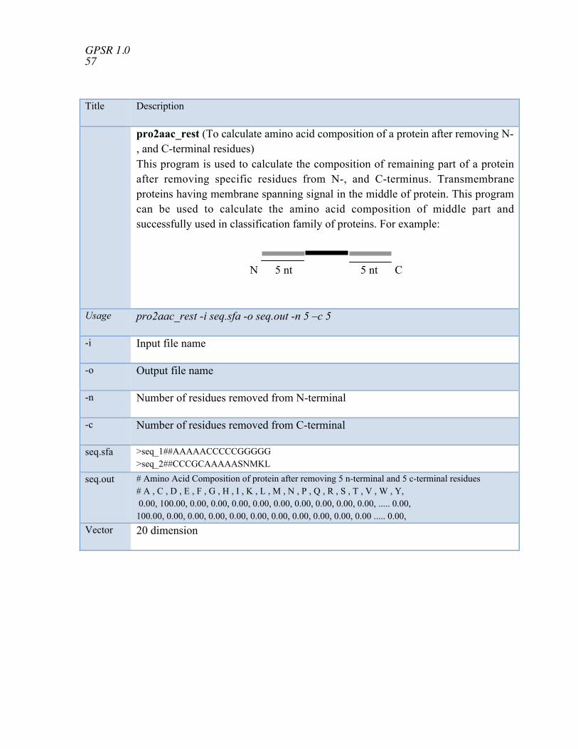
pro2aac_rest (To calculate amino acid composition of a protein after removing N-, and C-terminal residues)This program is used to calculate the composition of remaining part of a proteinafter removing specific residues from N-, and C-terminus. Transmembraneproteins having membrane spanning signal in the middle of protein. This programcan be used to calculate the amino acid composition of middle part andsuccessfully used in classification family of proteins. For example:

N 5 nt 5 nt C

Usage pro2aac_rest -i seq.sfa -o seq.out -n 5 –c 5

-i Input file name

-o Output file name

-n Number of residues removed from N-terminal

-c Number of residues removed from C-terminal

seq.sfa >seq_1##AAAAACCCCCGGGGG>seq_2##CCCGCAAAAASNMKL

seq.out # Amino Acid Composition of protein after removing 5 n-terminal and 5 c-terminal residues# A , C , D , E , F , G , H , I , K , L , M , N , P , Q , R , S , T , V , W , Y, 0.00, 100.00, 0.00, 0.00, 0.00, 0.00, 0.00, 0.00, 0.00, 0.00, 0.00, ..... 0.00,100.00, 0.00, 0.00, 0.00, 0.00, 0.00, 0.00, 0.00, 0.00, 0.00, 0.00 ..... 0.00,

Vector 20 dimension

GPSR 1.0 58

Title Description

pro2aac_split (To calculate split amino acid composition (SSAC) of aprotein)It has been reported that some sequence motifs are present into specific region of aprotein. Therefore, instead of computing the composition of whole sequence it isuseful to split the sequence into different equal parts. Composition of each part isseparately calculated, thus feature of region specific motifs is utilized, and addedto each other. Some reports show that is increases the prediction accuracy afterusing this strategy. The advantage of SSAC over standard amino acid compositionis that it provides greater weight to proteins that have a signal at either the N or Cterminus. For Example:

N C

Usage pro2aac_split -i seq.sfa -o seq.out -n 3

-i Input file name

-o Output file name

-n Number of parts split into, here 3 i.e. three equal parts of whole protein

seq.sfa >seq_1##AAAAACCCCCGGGGG>seq_2##CCCGCAAAAASNMKL

seq.out # Amino Acid Composition of 3 equal parts of proteins# A , C , D , E , F , G , H , I , K , L , M , N , P , Q , R , S , T , V , W , Y, 5.00, 0.00, 0.00, 0.00, 0.00, 0.00, 0.00, 0.00, 0.00, 0.00, 0.00, 0.00, 0.00, 0.00, 0.00, 0.00, 0.00,0.00, 0.00, 0.00, 0.00, 5.00, 0.00, 0.00, 0.00, 0.00, 0.00, 0.00, 0.00, 0.00, 0.00, 0.00, 0.00, 0.00,0.00, 0.00, 0.00, 0.00, 0.00, 0.00, 0.00, 0.00, 0.00, 0.00, 0.00, 5.00, 0.00, 0.00, 0.00, 0.00, 0.00,0.00, 0.00, 0.00, 0.00, 0.00, 0.00, 0.00, 0.00, 0.00, 0.00, 4.00, 0.00, 0.00, 0.00, 1.00, 0.00, 0.00, 0.00, 0.00, 0.00, 0.00, 0.00, 0.00, 0.00, 0.00, 0.00,0.00, 0.00, 0.00, 5.00, 0.00, 0.00, 0.00, 0.00, 0.00, 0.00, 0.00, 0.00, 0.00, 0.00, 0.00, 0.00, 0.00,0.00, 0.00, 0.00, 0.00, 0.00, 0.00, 0.00, 0.00, 0.00, 0.00, 0.00, 0.00, 0.00, 0.00, 1.00, 1.00, 1.00,1.00, 0.00, 0.00, 0.00, 1.00, 0.00, 0.00, 0.00, 0.00,

Vector 60 dimension (20*3 parts)

GPSR 1.0 59

Title Description

pro2dpc (To calculate dipeptide composition of protein)

The dipeptide composition in a protein is simply the percentage of the differentadjacent pairs of amino acids represented in a particular protein. The aim ofcalculating the composition of proteins is to transform the variable length of proteinsequences to fixed length feature vectors. This is an important and most crucial stepduring classification of proteins using machine-learning techniques because theyrequire fixed length patterns. In addition the conversion of a protein sequence to avector of 400 dimensions using dipeptide composition will encapsulate theproperties of the neighboring amino acids.

The composition of all 400 natural amino acids were calculated by using thefollowing equation

Total number of amino acid (i +1) x 100Composition of dipep (i +1) =

Total number of all possible dipeptides

Where dpep (i) is fraction or composition of dipeptide type i. Di and N are thenumber of dipeptide of type i and number of residues in protein i, respectively.

Usage pro2dpc -i seq.sfa -o seq.out-i Input file name-o Output file nameseq.sfa >seq_2##AAAAACCCCCGGGGG

seq.out #AA , AC , AD ,….., CC ,….., CG , ….. , GG ,….., YY,28.571, 7.143, 0.000, ….., 28.571,….., 7.143, ….., 28.571,….., 0.000

Vector 400 dimension (20*20)

A-A-A-A-A-C-C-C-C-C-G-G-G-G-GN C

GPSR 1.0 60

Title Description

pro2dpc_nt (To calculate dipeptide composition of N-terminal (nt)residues of a protein)It is well known that some proteins having N-terminal signal sequence which isresponsible to transport whole protein into their specific subcellular compartmentlike, lysosome, endoplasmic reticulum, mitochondria, and chloroplast. Evidencesindicate that divergent N-terminal sequences also do influence catalytic behavior,protein-protein interactions, and intracellular distributions of enzymes. Reportshows that N-terminal signal sequence can vary from 13 to 36 amino acid residuesin length and having all the information needed to localize into specific location.Therefore, N-terminal information could be exploited by using dipeptidecomposition feature to predict subcellular protein.

Usage pro2dpc_nt -i seq.sfa -o seq.out -n 5

-i Input file name

-o Output file name

-n Number of residues to calculate dipeptide composition from N-terminal

seq.sfa >seq_2##AAAAACCCCCGGGGG

Seq.out # Dipeptide composition of 5 n-terminal residues of proteins#AA , AC , AD ,….., CC ,….., CG , ….. , GG ,….., YY,100.00, 0.000, 0.000, ….., 00.000,….., 0.000, ….., 00.000,….., 0.000

Vector 400 dimension

GPSR 1.0 61

Title Description

pro2dpc_ct (To calculate dipeptide composition of C-terminal (ct)residues of a protein)

While the N-terminus of a protein often contains targeting signals, the C-terminuscan contain retention signals for protein sorting. The most common ER retentionsignal is the amino acid sequence -KDEL (or -HDEL) at the C-terminus, whichkeeps the protein in the endoplasmic reticulum and prevents it from entering thesecretory pathway. The C-terminus of proteins can be modified post-translationally,most commonly by the addition of a lipid anchor to the C-terminus that allows theprotein to be inserted into a membrane without having a transmembrane domain.The c-terminal domain of RNA polymerase II typically consists of up to 52 repeatsof the sequence Tyr-Ser-Pro-Thr-Ser-Pro-Ser. Other proteins often bind the C-terminal domain of RNA polymerase in order to activate polymerase activity. It isthe protein domain, which is involved in the initiation of DNA transcription, thecapping of the RNA transcript, and attachment to the spliceosome for RNAsplicing. Therefore the information at C-terminal in could be utilized usingdipeptide composition feature to predict different classes of proteins.

Usage pro2dpc_ct -i seq.sfa -o seq.out -n 5

-i Input file name

-o Output file name

-n Number of residues to calculate dipeptide composition from C-terminal

seq.sfa >seq_2##AAAAACCCCCGGGGG

Seq.out # Dipeptide composition of 5 n-terminal residues of proteins#AA , AC , AD ,….., CC ,….., CG , ….. , GG ,….., YY,100.00, 0.000, 0.000, ….., 00.000,….., 0.000, ….., 100.000,….., 0.000

Vector 400 dimension

GPSR 1.0 62

GPSR 1.0 63

Title Description

pro2tpc (To calculate tripeptide composition of protein)The tripeptide composition in a protein is simply the percentage of the threeadjacent amino acids represented in a particular protein. The aim of calculating thecomposition of proteins is to transform the variable length of protein sequences tofixed length feature vectors. This is an important and most crucial step duringclassification of proteins using machine-learning techniques because they requirefixed length patterns. In addition the conversion of a protein sequence to a vector of8000 dimensions using tripeptide composition will encapsulate the properties of theneighboring amino acids.

The composition of all 8000 natural amino acids were calculated by using thefollowing equation

Total number of amino acid (i +2) x 100Composition of tripep (i +2) =

Total number of all possible tripeptides

Usage pro2tpc -i seq.sfa -o seq.out

-i Input file name

-o Output file name

seq.sfa >seq_2##AAAAACCCCCGGGGG

Seq.out # Tripeptide Composition of Protein#AAA ,AAC ,AAD ,AAE ,AAF , …..,,YYW ,YYY23.0769 , 7.6923, 0.000, 00.000, 0.000, ….., 0.000 , 0.000

Vector 8000 dimension

A-A-A-A-A-C-C-C-C-C-G-G-G-G-GN C

GPSR 1.0 64

Title Description

add cols (To add columns of two files)It is used to make a hybrid method. In this two different features (e.g. amino acidcomposition, and dipeptided) of a sequence are added to make a more informative hybridfeatures.

Usage add_cols -i se1.out -c se2.out -o seq.out

-i Input file (first column file for add)

-c Input file (second column file for add)

-o Output file name

se1.out Amino Acid Composition of proteins# A , C , D , E , F , G , ….., Y,33.33,33.33, 0.00, 0.00, 0.00,33.33, ….., 0.00

se2.out # Dipeptide Composition of Protein#AA , AC , ….., YY28.571,7.143…..,0.00

seq.out # Amino Acid Composition of proteins # Dinucleic Composition of Protein# A , C , D , E , F , G , …., #AA , AC, .…, YY33.33,33.33, 0.00, 0.00, 0.00, 33.33,……, 28.571,7.143…..,0.00

Vector 420 (20 for amino acid + 400 dipeptide composition)

GPSR 1.0 65

Title Description

col2svm (To generating SVM_light input format)This program can convert composition output file into a format used in SVMtraining. In SVM format, (1) starts with +1 or –1 denotes class of sequencepositive or negative respectively. (2) A numerical order is given before each value.

Usage col2svm -i se1.out -o svm.out -s +1

-i Input file name

-o Output file name

-s Class for svm (+1 or –1)

se1.out Amino Acid Composition of proteins# A, C, D, E, F, G,… Y,33.33, 33.33, 0.00, 0.00, 0.00, 33.33, ….., 0.00

svm.out +1 1:33.330000 2:33.330000 3:0.000000 4:0.000000 5:0.000000 6:33.330000 ……. 20:0.000000

Vector 20 dimension

GPSR 1.0 66

GPSR 1.0 67

Title Description

col_mult (To multiplying each column of input file with a number)This program is used to multiply each column of input file with a specific number.This is used especially in the hybrid case to make the features equal weight.Suppose one wants to make a hybrid file of amino acid and dipeptide composition.If amino acid and dipeptide composition was added directly the values ofmononucleotide is very high with respect to dinucleotide. Thus performance ofSVM will be nearly similar to the performance of amino acid because the weightof dipeptide is diluted. But when we multiply the amino acid with 10 or dipeptidewith 0.1 and then added to each other. There is chance that performance willincrease.

Usage col_mult -i se1.out -o se1_mult -n 0.1

-i Input file name

-o Output file name

-n Number with which column is multiplying

se1.out Amino Acid Composition of proteins# A , C , D , E , F , G , ….., Y,33.33, 33.33, 0.00, 0.00, 0.00, 33.33, ….., 0.00

se1_mult 3.333000, 3.333000, 0.000000, 0.000000, 0.000000, 3.333000,….. , 0.000000,

Vector Same as in input file

GPSR 1.0 68

Title Description

col_mult_sel (To multiplying selective columns with a number)

Instead of multiplying whole column, here only column from 1 to 3 are multipliedwith specific number (10).

Usage col_mult_sel -i se1.out -o se1_mult -n 10 -a 1 -b 3

-i Input file name

-o Output file name

-n Number with which column is multiplying

-a Number of starting column (eg 1)

-b Number of last column (eg 3)

se1.out Amino Acid Composition of proteins# A , C , D , E , F , G , ….., Y,33.33, 33.33, 0.00, 0.00, 0.00, 33.33, ….., 0.00

se1_mult 333.300000, 333.300000, 0.000000, 0.000000, 0.000000, 33.330000,….., 0.000000

Vector Same as in input file

GPSR 1.0 69

GPSR 1.0 70

Title Description

perl col_rem (To remove selective columns from a file)This program is used to remove specific column from files. You can remove thecomposition of A and C from whole file to check the importance of these aminoacids in prediction methods.

Usage perl col_rem -i seq.out -o seq.rm -a 1 -b 2

-i Input file name

-o Output file name

-a Number of starting column (eg 1) to removed

-b Number of last column (eg 3) removed

seq.out # Amino Acid Composition of proteins# A , C , D , E , F , G , H , I , K , L , M , N , P , Q , R , S , T , V , W , Y,18.60, 2.33, 4.65, 5.81, 5.81, 8.14, 1.16, 1.16, 0.00, 8.14, 3.49, 1.16, 3.49, 0.00, 13.95, 4.65, 8.14,5.81, 0.00, 3.49,

Seq_rm 5.810000,5.810000,8.140000,1.160000,1.160000,0.000000,8.140000,3.490000,1.160000,3.490000,0.000000,13.950000,4.650000,8.140000,5.810000,0.000000,3.490000

Vector Total number = Total columns in the input file – total number of removed columnE.g.(17=20-3)

GPSR 1.0 71

Title Description

col_ext (To extract selective columns from a file)This program only takes specific column from a file. In this example we only takethe feature of amino acid composition of F, G, H, I, and K as an input for SVM.

Usage col_ext -i seq.out -o seq.ext -a 5 -b 10

-i Input file name

-o Output file name

-a Number of starting column (eg 5) to take

-b Number of last column (eg 10) to take

seq.out # Amino Acid Composition of proteins# A , C , D , E , F , G , H , I , K , L , M , N , P , Q , R , S , T , V , W , Y,18.60, 2.33, 4.65, 5.81, 5.81, 8.14, 1.16, 1.16, 0.00, 8.14, 3.49, 1.16, 3.49, 0.00, 13.95, 4.65, 8.14,5.81, 0.00, 3.49,

Seq.ext 5.81, 8.14, 1.16, 1.16, 0.00, 8.14

Vector Total number = Total number of column selected from input fileEg(6=from 5 to 10 colum)

GPSR 1.0 72

Title Description

col_corr (To compute correlation co-efficient between two column)Correlation co-efficient indicates the strength and direction of a linearrelationship between two random variables. The correlation varies between –1 to1. The closer the coefficient is to either -1 or 1, the stronger the correlationbetween the variables. Value of 1 in the case of an increasing linear relationship, -1 in the case of a decreasing linear relationship, 0 in case no correlation. Exampleshows the correlation between amino acid A and G in the file.

Usage col_corr -i pos -a 1 -b 6

-i Input file name

-a Number of column (eg 1)

-b Number of column (eg 6)

pos # Amino Acid Composition of proteins# A , C , D , E , F , G , H , I , K , L , M , N , P , Q , R , S , T , V , W , Y,15.31, 1.30, 7.49, 3.91, 2.28, 9.45, 1.63, 3.26, 1.95, 10.10, 1.95, 2.28, 5.54, 2.28, 8.14, 3.91, 8.47,6.84, 0.98, 2.93,15.31, 1.30, 7.49, 3.91, 2.28, 9.45, 1.63, 3.26, 1.95, 10.10, 1.95, 2.28, 5.54, 2.28, 8.14, 3.91, 8.47,6.84, 0.98, 2.93,12.83, 1.60, 8.56, 2.14, 2.67, 6.95, 6.95, 2.67, 1.60, 9.09, 3.74, 3.74, 6.42, 6.42, 4.28, 5.35, 6.42,5.35, 1.07, 2.14,12.30, 1.60, 8.56, 2.14, 2.67, 6.95, 6.95, 2.67, 1.60, 9.09, 3.74, 3.74, 6.42, 6.42, 4.28, 5.35, 6.42,5.88, 1.07, 2.14,13.76, 0.53, 4.76, 4.23, 3.70, 5.29, 1.06, 3.17, 2.12, 8.47, 3.17, 3.70, 13.76, 1.59, 4.76, 9.52, 8.99,5.82, 1.06, 0.53,

output 0.749 (a positive correlation between column 1 and 6)

Vector Total number = Total number of column selected from input fileE.g.(6=from 5 to 10 colum)

GPSR 1.0 73

Title Description

col_avg (To calculate average column of two files)In this case composition value of each column of a file is added to itscorresponding column of another file and means value is calculated. It can beused to generate an average feature of two different files (belonging from samefamily of protein) to make input in machine learning techniques. For instance,15.31 (1st column of file pos1) + 6.87 (1st column of file pos2) = 22.18/2 = 11.09(file out).Note: Each file should have equal number of columns and rows

Usage col_avg -a pos1 -b pos2 -o out-a First input file name-b Second input file name-o Output file namepos1 # Amino Acid Composition of proteins

# A , C , D , E , F , G , H , I , K , L , M , N , P , Q , R , S , T , V , W , Y,15.31, 1.30, 7.49, 3.91, 2.28, 9.45, 1.63, 3.26, 1.95,10.10, 1.95, 2.28, 5.54, 2.28, \8.14, 3.91, 8.47, 6.84, 0.98, 2.93,15.31, 1.30, 7.49, 3.91, 2.28, 9.45, 1.63, 3.26, 1.95,10.10, 1.95, 2.28, 5.54, 2.28, \8.14, 3.91, 8.47, 6.84, 0.98, 2.93,12.83, 1.60, 8.56, 2.14, 2.67, 6.95, 6.95, 2.67, 1.60, 9.09, 3.74, 3.74, 6.42, 6.42, \4.28, 5.35, 6.42, 5.35, 1.07, 2.14,

pos2 # Amino Acid Composition of proteins# A , C , D , E , F , G , H , I , K , L , M , N , P , Q , R , S , T , V , W , Y,6.87, 1.29, 6.87, 2.15, 0.86, 6.87, 1.72, 4.72, 5.58, 9.87, 1.29, 5.15, 4.72, 5.15, 1.72,13.73,9.01,10.30, 1.72, 0.43,9.87, 1.29, 7.30, 3.00, 0.86, 8.58, 1.29, 4.72, 4.29, 9.87, 0.86, 3.43, 5.15, 4.29, 3.43,11.16, 7.73,10.73, 1.72, 0.43,12.64, 1.10, 4.40, 1.10, 2.75, 9.34, 0.55, 6.59, 3.30, 9.34, 2.20, 6.59, 6.04, 5.49, 4.40, 6.59, 7.14,9.34, 0.55, 0.55,

out 11.09; 1.295; 7.18; 3.03; 1.57; 8.16; 1.675; 3.99; 3.765; 9.985; 1.62; 3.715; 5.13; 3.715; 4.93;8.82; 8.74; 8.57; 1.35; 1.68; 012.59; 1.295; 7.395; 3.455; 1.57; 9.015; 1.46; 3.99; 3.12; 9.985; 1.405; 2.855; 5.345; 3.285; 5.785;7.535; 8.1; 8.785; 1.35; 1.68; 012.735; 1.35; 6.48; 1.62; 2.71; 8.145; 3.75; 4.63; 2.45; 9.215; 2.97; 5.165; 6.23; 5.955; 4.34; 5.97;6.78; 7.345; 0.81; 1.345; 0

Vector Total number of column (same as in input file)

GPSR 1.0 74

Title Description

seq2pssm_imp (To calculate PSSM matrix in column format withoutany normalization)The PSSM for each sequence was generated by performing PSI-BLAST searchagainst specific database (e.g. nr) using different iterations (e.g. 3) with cut off e-value 0.001. For a sequence of length N residues, PSSM is represented by anNX20 matrix. Each element of this matrix, m [i, j], provides information onevolutionary conservation of residue type j at sequence position i. For example:

Usage seq2pssm_imp -i seq1.fa -o pssm.out –d nr-i Input file in the fasta format (not use single fasta format)-o Output file-d Database against which PSSM profile is generatedseq1.fa >1BISA PDBID CHAIN_SEQUENC

GSHMHGQVDCSPGIWQLDCTHLEGKVILVAVHVASGYIEAEVIPAETGQETAYFLLKLAGRWPVKTVHTDNGSNFTSTTVKAACEWAGIKQEFGIPYNPQSQGVIESMNKELK

pssm.out G, 0, -300, -100, -200, -300, 599, -200, -400, -200, -400, -300, 0, -200, -200, -200, 0, -200, -300, -200, -300S, 100, -100, 0, 0, -200, 0, -100, -200, 0, -200, -100, 100, -100, 0, -100, 400, 100, -200, -300, -200H, -200, -300, -100, 0, -100, -200, 799, -300, -100, -300, -200, 100, -200, 0, 0, -100, -200, -300, -200, 200M, -100, -100, -300, -200, 0, -300, -200, 100, -100, 200, 499, -200, -200, 0, -100, -100, -100, 100,-100, -100H, -200, -300, -100, 0, -100, -200, 799, -300, -100, -300, -200, 100, -200, 0, 0, -100, -200,\-300, -200, 200

GPSR 1.0 75

G, 0, -300, -100, -200, -300, 599, -200, -400, -200, -400, -300, 0, -200, -200, -200, 0, -200, -300, -200, -300Q, -100, -300, 0, 200, -300, -200, 0, -300, 100, -200, 0, 0, -100, 499, 100, 0, -100, -200, -200, -100……….

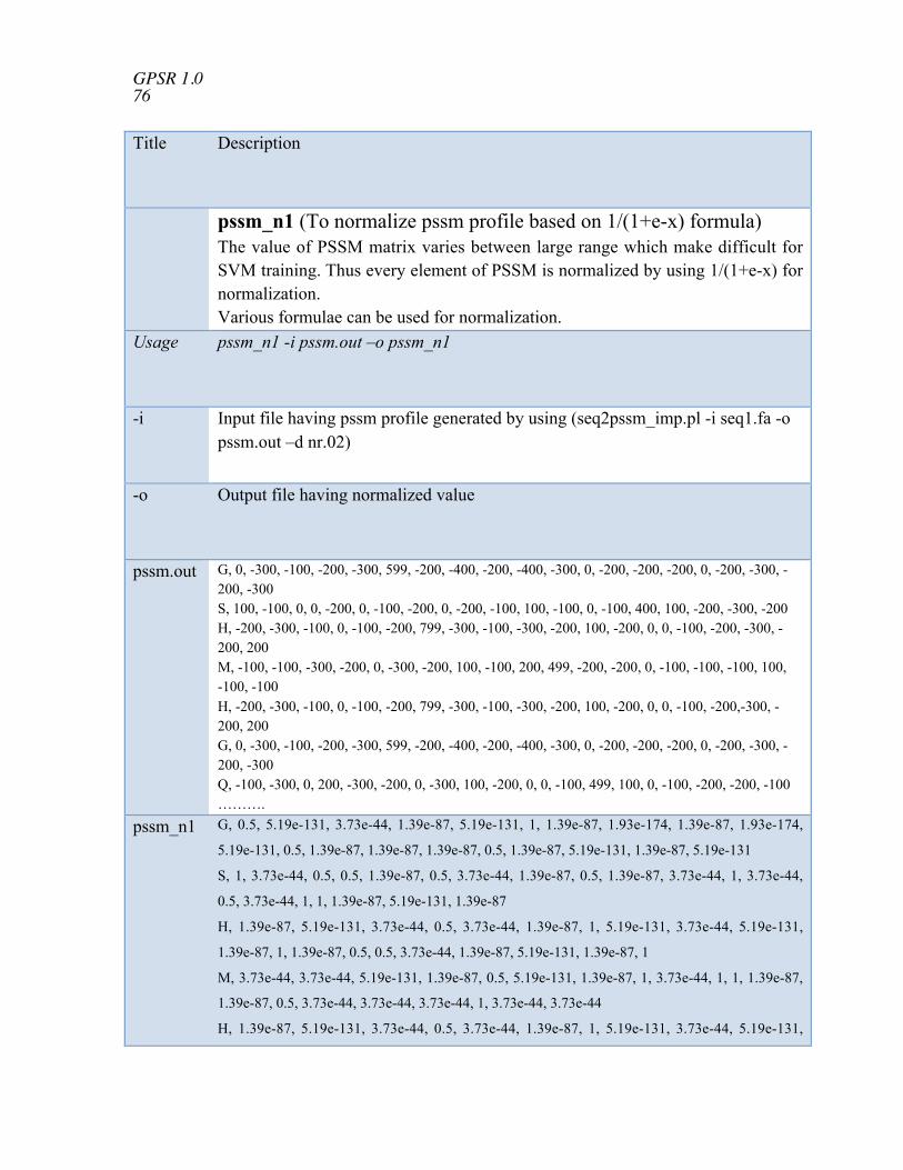
GPSR 1.0 76

Title Description

pssm_n1 (To normalize pssm profile based on 1/(1+e-x) formula)The value of PSSM matrix varies between large range which make difficult forSVM training. Thus every element of PSSM is normalized by using 1/(1+e-x) fornormalization.Various formulae can be used for normalization.

Usage pssm_n1 -i pssm.out –o pssm_n1

-i Input file having pssm profile generated by using (seq2pssm_imp.pl -i seq1.fa -opssm.out –d nr.02)

-o Output file having normalized value

pssm.out G, 0, -300, -100, -200, -300, 599, -200, -400, -200, -400, -300, 0, -200, -200, -200, 0, -200, -300, -200, -300S, 100, -100, 0, 0, -200, 0, -100, -200, 0, -200, -100, 100, -100, 0, -100, 400, 100, -200, -300, -200H, -200, -300, -100, 0, -100, -200, 799, -300, -100, -300, -200, 100, -200, 0, 0, -100, -200, -300, -200, 200M, -100, -100, -300, -200, 0, -300, -200, 100, -100, 200, 499, -200, -200, 0, -100, -100, -100, 100,-100, -100H, -200, -300, -100, 0, -100, -200, 799, -300, -100, -300, -200, 100, -200, 0, 0, -100, -200,-300, -200, 200G, 0, -300, -100, -200, -300, 599, -200, -400, -200, -400, -300, 0, -200, -200, -200, 0, -200, -300, -200, -300Q, -100, -300, 0, 200, -300, -200, 0, -300, 100, -200, 0, 0, -100, 499, 100, 0, -100, -200, -200, -100……….

pssm_n1 G, 0.5, 5.19e-131, 3.73e-44, 1.39e-87, 5.19e-131, 1, 1.39e-87, 1.93e-174, 1.39e-87, 1.93e-174,

5.19e-131, 0.5, 1.39e-87, 1.39e-87, 1.39e-87, 0.5, 1.39e-87, 5.19e-131, 1.39e-87, 5.19e-131

S, 1, 3.73e-44, 0.5, 0.5, 1.39e-87, 0.5, 3.73e-44, 1.39e-87, 0.5, 1.39e-87, 3.73e-44, 1, 3.73e-44,

0.5, 3.73e-44, 1, 1, 1.39e-87, 5.19e-131, 1.39e-87

H, 1.39e-87, 5.19e-131, 3.73e-44, 0.5, 3.73e-44, 1.39e-87, 1, 5.19e-131, 3.73e-44, 5.19e-131,

1.39e-87, 1, 1.39e-87, 0.5, 0.5, 3.73e-44, 1.39e-87, 5.19e-131, 1.39e-87, 1

M, 3.73e-44, 3.73e-44, 5.19e-131, 1.39e-87, 0.5, 5.19e-131, 1.39e-87, 1, 3.73e-44, 1, 1, 1.39e-87,

1.39e-87, 0.5, 3.73e-44, 3.73e-44, 3.73e-44, 1, 3.73e-44, 3.73e-44

H, 1.39e-87, 5.19e-131, 3.73e-44, 0.5, 3.73e-44, 1.39e-87, 1, 5.19e-131, 3.73e-44, 5.19e-131,

1.39e-87, 1, 1.39e-87, 0.5, 0.5, 3.73e-44, 1.39e-87, 5.19e-131, 1.39e-87, 1

GPSR 1.0 77

1.39e-87, 1, 1.39e-87, 0.5, 0.5, 3.73e-44, 1.39e-87, 5.19e-131, 1.39e-87, 1

G, 0.5, 5.19e-131, 3.73e-44, 1.39e-87, 5.19e-131, 1, 1.39e-87, 1.93e-174, 1.39e-87, 1.93e-174,

5.19e-131, 0.5, 1.39e-87, 1.39e-87, 1.39e-87, 0.5, 1.39e-87, 5.19e-131, 1.39e-87, 5.19e-131

Q, 3.73e-44, 5.19e-131, 0.5, 1, 5.19e-131, 1.39e-87, 0.5, 5.19e-131, 1, 1.39e-87, 0.5, 0.5, 3.73e-

44, 1, 1, 0.5, 3.73e-44, 1.39e-87, 1.39e-87, 3.73e-44

GPSR 1.0 78

Title Description

pssm_n2 (To normalize pssm profile based on (numb -min)/(max -min) formula)

The value of PSSM matrix varies between large range which make difficult forSVM training. Thus every element of PSSM is normalized by using (numb -min)/(max -min) for normalization. For example:

Usage pssm_n2 -i pssm.out –o pssm_n2

-i Input file having pssm profile generated by using (seq2pssm_imp.pl -i seq1.fa -opssm.out –d nr.02)

GPSR 1.0 79

-o Output file having normalized value

pssm.out G, 0, -300, -100, -200, -300, 599, -200, -400, -200, -400, -300, 0, -200, -200, -200, 0, -200, -300, -200, -300S, 100, -100, 0, 0, -200, 0, -100, -200, 0, -200, -100, 100, -100, 0, -100, 400, 100, -200, -300, -200H, -200, -300, -100, 0, -100, -200, 799, -300, -100, -300, -200, 100, -200, 0, 0, -100, -200, -300, -200, 200M, -100, -100, -300, -200, 0, -300, -200, 100, -100, 200, 499, -200, -200, 0, -100, -100, -100, 100,-100, -100H, -200, -300, -100, 0, -100, -200, 799, -300, -100, -300, -200, 100, -200, 0, 0, -100, -200,-300, -200, 200G, 0, -300, -100, -200, -300, 599, -200, -400, -200, -400, -300, 0, -200, -200, -200, 0, -200, -300, -200, -300Q, -100, -300, 0, 200, -300, -200, 0, -300, 100, -200, 0, 0, -100, 499, 100, 0, -100, -200, -200, -100……….

pssm_n2 G, 0.26, 0.06, 0.20, 0.13, 0.06, 0.66, 0.13, 0, 0.13, 0, 0.06, 0.26, 0.13, 0.13, 0.13, 0.26, 0.13, 0.06,

0.13, 0.06

S, 0.33, 0.20, 0.26, 0.26, 0.13, 0.26, 0.20, 0.13, 0.26, 0.13, 0.20, 0.33, 0.20, 0.26, 0.20, 0.53, 0.33,

0.13, 0.06, 0.13

H, 0.13, 0.06, 0.20, 0.26, 0.20, 0.13, 0.79, 0.06, 0.20, 0.06, 0.13, 0.33, 0.13, 0.26, 0.26, 0.20, 0.13,

0.06, 0.13, 0.40

M, 0.20, 0.20, 0.06, 0.13, 0.26, 0.06, 0.13, 0.33, 0.20, 0.40, 0.59, 0.13, 0.13, 0.26, 0.20, 0.20, 0.20,

0.33, 0.20, 0.20

H, 0.13, 0.06, 0.20, 0.26, 0.20, 0.13, 0.79, 0.06, 0.20, 0.06, 0.13, 0.33, 0.13, 0.26, 0.26, 0.20, 0.13,

0.06, 0.13, 0.40

G, 0.26, 0.06, 0.20, 0.13, 0.06, 0.66, 0.13, 0, 0.13, 0, 0.06, 0.26, 0.13, 0.13, 0.13, 0.26, 0.13, 0.06,

0.13, 0.06

Q, 0.20, 0.06, 0.26, 0.40, 0.06, 0.13, 0.26, 0.06, 0.33, 0.13, 0.26, 0.26, 0.20, 0.59, 0.33, 0.26, 0.20,0.13, 0.13, 0.2

GPSR 1.0 80

Title Description

pssm_n3 (To normalize pssm profile based on (numb -min)*100/(max-min) formula)The value of PSSM matrix varies between large ranges which make difficult forSVM training. Thus every element of PSSM is normalized by using (numb -min)*100/(max -min)for normalization.

Usage pssm_n3 -i pssm.out –o pssm_n3-i Input file having pssm profile generated by using (seq2pssm_imp.pl -i seq1.fa -o

pssm.out –d nr.02)

-o Output file having normalized valuepssm.out G, 0, -300, -100, -200, -300, 599, -200, -400, -200, -400, -300, 0, -200, -200, -200, 0, -200, -300, -

200, -300S, 100, -100, 0, 0, -200, 0, -100, -200, 0, -200, -100, 100, -100, 0, -100, 400, 100, -200, -300, -200H, -200, -300, -100, 0, -100, -200, 799, -300, -100, -300, -200, 100, -200, 0, 0, -100, -200, -300, -200, 200M, -100, -100, -300, -200, 0, -300, -200, 100, -100, 200, 499, -200, -200, 0, -100, -100, -100, 100, -100, -100H, -200, -300, -100, 0, -100, -200, 799, -300, -100, -300, -200, 100, -200, 0, 0, -100, -200,-300, -200, 200G, 0, -300, -100, -200, -300, 599, -200, -400, -200, -400, -300, 0, -200, -200, -200, 0, -200, -300, -200, -300Q, -100, -300, 0, 200, -300, -200, 0, -300, 100, -200, 0, 0, -100, 499, 100, 0, -100, -200, -200, -100

pssm_n3 G, 26.68, 6.67, 20.01, 13.34, 6.67, 66.64, 13.34, 0, 13.34, 0, 6.67, 26.68, 13.34, 13.34, 13.34,

26.68, 13.34, 6.67, 13.34, 6.67

S, 33.35, 20.01, 26.68, 26.68, 13.34, 26.68, 20.01, 13.34, 26.68, 13.34, 20.01, 33.35, 20.01, 26.68,

20.01, 53.36, 33.35, 13.34, 6.67, 13.34

H, 13.34, 6.67, 20.01, 26.68, 20.01, 13.34, 79.98, 6.67, 20.01, 6.67, 13.34, 33.35, 13.34, 26.68,

26.68, 20.01, 13.34, 6.67, 13.34, 40.02

M, 20.01, 20.01, 6.67, 13.34, 26.68, 6.67, 13.34, 33.35, 20.01, 40.02, 59.97, 13.34, 13.3, 26.68,

20.01, 20.01, 20.01, 33.35, 20.01, 20.01

H, 13.34, 6.67, 20.01, 26.68, 20.01, 13.34, 79.98, 6.67, 20.01, 6.67, 13.34, 33.35, 13.34, 26.68,

26.68, 20.01, 13.34, 6.67, 13.34, 40.02

G, 26.68, 6.67, 20.01, 13.34, 6.67, 66.64, 13.34, 0, 13.34, 0, 6.67, 26.68, 13.34, 13.34, 13.34,

26.68, 13.34, 6.67, 13.34, 6.67

Q, 20.01, 6.67, 26.68, 40.02, 6.67, 13.34, 26.68, 6.67, 33.35, 13.34, 26.68, 26.68, 20.01, 59.97,33.35, 26.68, 20.01, 13.34

GPSR 1.0 81

Title Description

pssm_n4 (To normalize pssm profile based on 1/(1+e-(x/100)formula)The value of PSSM matrix varies between large range which make difficult forSVM training. Thus every element of PSSM is normalized by using 1/(1+e-(x/100) for normalization.

Usage pssm_n4 -i pssm.out –o pssm_n4-i Input file having pssm profile generated by using (seq2pssm_imp.pl -i seq1.fa -o

pssm.out –d nr.02)-o Output file having normalized valuepssm.out G, 0, -300, -100, -200, -300, 599, -200, -400, -200, -400, -300, 0, -200, -200, -200, 0, -

200, -300, -200, -300S, 100, -100, 0, 0, -200, 0, -100, -200, 0, -200, -100, 100, -100, 0, -100, 400, 100, -200, -300, -200H, -200, -300, -100, 0, -100, -200, 799, -300, -100, -300, -200, 100, -200, 0, 0, -100, -200, -300, -200, 200M, -100, -100, -300, -200, 0, -300, -200, 100, -100, 200, 499, -200, -200, 0, -100, -100, -100, 100, -100, -100H, -200, -300, -100, 0, -100, -200, 799, -300, -100, -300, -200, 100, -200, 0, 0, -100, -200,-300, -200, 200G, 0, -300, -100, -200, -300, 599, -200, -400, -200, -400, -300, 0, -200, -200, -200, 0, -200, -300, -200, -300Q, -100, -300, 0, 200, -300, -200, 0, -300, 100, -200, 0, 0, -100, 499, 100, 0, -100, -200, -200, -100……….

pssm_n4 G, 0.5, 0.04, 0.26, 0.11, 0.04, 0.99, 0.11, 0.01, 0.11, 0.01, 0.0474258731775668, 0.5, 0.11, 0.11,

0.11, 0.5, 0.11, 0.047, 0.11, 0.04

S, 0.73, 0.26, 0.5, 0.5, 0.11, 0.5, 0.26, 0.11, 0.5, 0.11, 0.26, 0.73, 0.26, 0.5, 0.26, 0.98, 0.73, 0.11,

0.04, 0.11

H, 0.11, 0.04, 0.26, 0.5, 0.26, 0.11, 0.99, 0.04, 0.26, 0.04, 0.11, 0.73, 0.119202922022118, 0.5,

0.5, 0.26, 0.11, 0.04, 0.11, 0.88

M, 0.26, 0.26, 0.04, 0.11, 0.5, 0.04, 0.11, 0.73, 0.26, 0.88, 0.99, 0.11, 0.11, 0.5, 0.26, 0.26, 0.26,

0.73, 0.26, 0.26

H, 0.11, 0.047, 0.26, 0.5, 0.26, 0.11, 0.99, 0.047, 0.26, 0.04, 0.11, 0.73, 0.11, 0.5, 0.5, 0.26, 0.11,

0.04, 0.11, 0.88

G, 0.5, 0.04, 0.26, 0.11, 0.04, 0.99, 0.11, 0.01, 0.11, 0.01, 0.04, 0.5, 0.11, 0.11, 0.11, 0.5, 0.11,

0.04, 0.11, 0.04

Q, 0.26, 0.04, 0.5, 0.88, 0.04, 0.11, 0.5, 0.04, 0.73, 0.11, 0.5, 0.5, 0.26, 0.99, 0.73, 0.5, 0.26, 0.11,

0.11, 0.26

GPSR 1.0 82

Title Description

pssm_comp (To compute PSSM composition (400 points))Here pssm matrix is coverted in a vector of dimension 400, by computingcomposition of occurrences of each type of amino acid corresponding to eachtype of amino acids in protein sequence. It means for each column we willhave 20 values instead of one. Every element in this input vector wassubsequently divided by the length of the sequence. The resultant matrix with400 elements was used as input feature for SVM.

Usage pssm_comp -i pssm_n4 –o pssm_n4.out

-i Input file having pssm profile generated by using (seq2pssm_imp -i seq1.fa–o pssm.out –d nr.02) and then scaled by using (pssm_n4.pl -i pssm.out –opssm_n4)

-o Output file having 400 elementspssm_n4 G, 0.5, 0.04, 0.26, 0.11, 0.04, 0.99, 0.11, 0.01, 0.11, 0.01, 0.04, 0.5, 0.11, 0.11, 0.11, 0.5,

0.11, 0.04, 0.11, 0.04

S, 0.73, 0.26, 0.5, 0.5, 0.11, 0.5, 0.26, 0.11, 0.5, 0.11, 0.26, 0.73, 0.26, 0.5, 0.26, 0.98, 0.73,

0.11, 0.04, 0.11

H, 0.11, 0.04, 0.26, 0.5, 0.26, 0.11, 0.99, 0.047, 0.26, 0.047, 0.11, 0.73, 0.11, 0.5, 0.5, 0.26,

0.11, 0.04, 0.11, 0.88

M, 0.26, 0.26, 0.04, 0.11, 0.5, 0.04, 0.11, 0.73, 0.26, 0.88, 0.99, 0.11, 0.11, 0.5, 0.26, 0.26,

0.26, 0.73, 0.26, 0.26

H, 0.11, 0.04, 0.26, 0.5, 0.26, 0.11, 0.99, 0.04, 0.26, 0.04, 0.11, 0.73, 0.11, 0.5, 0.5, 0.26,

0.11, 0.04, 0.11, 0.88

G, 0.5, 0.04, 0.26, 0.11, 0.04, 0.99, 0.11, 0.01, 0.11, 0.01, 0.04, 0.5, 0.11, 0.11, 0.11, 0.5,

0.11, 0.04, 0.11, 0.04

Q, 0.26, 0.04, 0.5, 0.88, 0.04, 0.11, 0.5, 0.04, 0.73, 0.11, 0.5, 0.5, 0.26, 0.99, 0.73, 0.5, 0.26,

0.11, 0.11, 0.26

pssm_n4.out 0.98, 0.50, 0.11, 0.26, 0.11, 0.50, 0.11, 0.26, 0.26, 0.26, 0.26, 0.11, 0.26, 0.26894142, 0.26,0.73, 0.50, 0.50, 0.04, 0.11, 0.50, 0.99, 0.04, 0.01, 0.11, 0.04, 0.04, 0.26, 0.04, 0.26, 0.26,0.04, 0.04, 0.04, 0.04, 0.26, 0.26, 0.26, 0.11, 0.11, ……..

Vector 400

GPSR 1.0 83

Title Description

col_sig (significance of columns in two column files)This program used to calculate significant of each column in two different file. Ifany one want to compare the positive and negative file of amino acid composition.Like Differences in positive-negative, its significance, average of each colomn inpositive and each column in negative, standard deviation. Output result will givecomparison of each column.

Usage col_sig -i file1 -j file2 >out

-i Input file1 of positive example-j Input file2 of negative examplefile1 # Amino Acid Composition of proteins

# A , C , D , E , F , G , H , I , K , L , M , N , P , Q , R , S , T , V , W , Y

7.88,1.27,4.05,6.39,3.62,7.88,2.13,6.61,5.75,10.23,3.62,2.98,3.41,5.11,5.54,6.39,4.47,7.03,1.70,3.83

5.46,1.12,7.14,6.72,3.78,5.46,1.68,4.76,6.58,10.64,0.98,7.42,2.52,4.06,4.90,9.38,8.54,5.04,0.98,2.80

8.96,2.06,4.82,7.58,4.13,6.20,0.69,4.82,7.58,13.10,1.37,2.75,4.82,8.96,6.89,4.13,2.75,6.20,0.00,2.64

file2 # Amino Acid Composition of proteins

# A , C , D , E , F , G , H , I , K , L , M , N , P , Q , R , S , T , V , W , Y

8.55,0.65,3.94,9.86,2.63,8.55,0.00,3.28,11.84,13.81,2.63,3.28,1.31,3.94,3.94,6.57,1.31,8.55,0.65,1.89

13.29,2.53,3.16,2.53,5.69,14.55,1.89,5.69,3.16,6.32,3.16,3.16,6.96,2.53,6.32,6.32,2.53,6.32,3.16,2.18

9.88,0.48,7.45,8.91,5.18,3.56,0.48,4.70,11.02,9.88,2.10,6.48,3.89,4.21,3.24,5.99,5.02,2.91,0.16,4.87

out # Parameters Measured: % Difference, Significance, Average1, Average2, Standard Deviation(SD1),

SD2

Column 1: -34.83, -490.31, 7.43, 10.57, 0.88, 0.39

Column 2: 19.44, 69.33, 1.48, 1.22, 0.33, 0.42

Column 3: 9.51, 53.98, 5.34, 4.85, 0.29, 1.50

Column 4: -2.89, -28.15, 6.90, 7.10, 0.39, 1.04

Column 5: -15.71, -234.15, 3.84, 4.50, 0.16, 0.39

Column 6: -30.79, -145.77, 6.51, 8.89, 0.18, 3.07

Column 7: 61.49, 218.36, 1.50, 0.79, 0.46, 0.17

Column 8: 16.83, 408.83, 5.4, 4.56, 0.33, 0.07

Column 9: -26.55, -214.22, 6.64, 8.67, 0.54, 1.35

Column 10: 12.34, 240.14, 11.32, 10.01, 1.02, 0.07

Column 11: -27.64, -193.90, 1.99, 2.63, 0.35, 0.30

Column 12: 1.76, 6.98, 4.38, 4.31, 0.94, 1.25

Column 13: -12.27, -115.47, 3.58, 4.05, 0.71, 0.09

Column 14: 51.68, 241.21, 6.04, 3.56, 1.68, 0.37

GPSR 1.0 84

Column 15: 24.79, 185.57, 5.78, 4.50, 0.64, 0.73

Column 16: 5.22, 41.72, 6.63, 6.30, 1.44, 0.17

Column 17: 56.04, 174.63, 5.26, 2.95, 1.44, 1.19

Column 18: 2.69, 17.94, 6.09, 5.93, 0.06, 1.74

Column 19: -38.94, -72.75, 0.89, 1.32, 0.516, 0.67

Column 20: 3.47, 15.63, 3.093, 2.98, 0.26, 1.09

GPSR 1.0 85

Title Description

pssm2pat (To generate patterns of given size from PSSM matrix)Here we generate PSSM matrix from different window size. If we want to generate 5-window matrix, take two nucleotide matrix forms upstream and downstream and concatenates all matrix in sequential order. For example: pattern matrix of GSHMH, add matrix of each nucleotide it makesthe 100 vector long matrix representing H (middle) of nucleotide. For starting nucleotide zero (0) is considered

Usage pssm2pat -i pssm.out –o pssm_pat –w 5-i Input file having pssm profile generated by using (seq2pssm_imp.pl -i seq1.fa -o pssm.out –d nr.02)-o Output file

-w Window size generated from PSSM matrixpssm.out G, 0, -300, -100, -200, -300, 599, -200, -400, -200, -400, -300, 0, -200, -200, -200, 0, -200, -300, -200, -300

S, 100, -100, 0, 0, -200, 0, -100, -200, 0, -200, -100, 100, -100, 0, -100, 400, 100, -200, -300, -200H, -200, -300, -100, 0, -100, -200, 799, -300, -100, -300, -200, 100, -200, 0, 0, -100, -200, -300, -200, 200M, -100, -100, -300, -200, 0, -300, -200, 100, -100, 200, 499, -200, -200, 0, -100, -100, -100, 100, -100, -100H, -200, -300, -100, 0, -100, -200, 799, -300, -100, -300, -200, 100, -200, 0, 0, -100, -200, -300, -200, 200G, 0, -300, -100, -200, -300, 599, -200, -400, -200, -400, -300, 0, -200, -200, -200, 0, -200, -300, -200, -300Q, -100, -300, 0, 200, -300, -200, 0, -300, 100, -200, 0, 0, -100, 499, 100, 0, -100, -200, -200, -100

pssm_pat # Pattern Window size 5 generated from PSSM matrix. Each line represents pattern for central residue0,0,0,0,0,0,0,0,0,0,0,0,0,0,0,0,0,0,0,0,0,0,0,0,0,0,0,0,0,0,0,0,0,0,0,0,0,0,0,0,0,-300,-100,-200,-300,599,-200,-400,-200,-400,-300,0,-200,-200,-200,0,-200,-300,-200,-300,100,-100,0,0,-200,0,-100,-200,0,-200,-100,100,-100,0,-100,400,100,-200,-300,-200,-200,-300,-100,0,-100,-200,799,-300,-100,-300,-200,100,-200,0,0,-100,-200,-300,-200,2000,0,0,0,0,0,0,0,0,0,0,0,0,0,0,0,0,0,0,0,0,-300,-100,-200,-300,599,-200,-400,-200,-400,-300,0,-200,-200,-200,0,-200,-300,-200,-300,100,-100,0,0,-200,0,-100,-200,0,-200,-100,100,-100,0,-100,400,100,-200,-300,-200,-200,-300,-100,0,-100,-200,799,-300,-100,-300,-200,100,-200,0,0,-100,-200,-300,-200,200,-100,-100,-300,-200,0,-300,-200,100,-100,200,499,-200,-200,0,-100,-100,-100,100,-100,-100

…………………………………………………

Vector 20*window size (20*5=100)

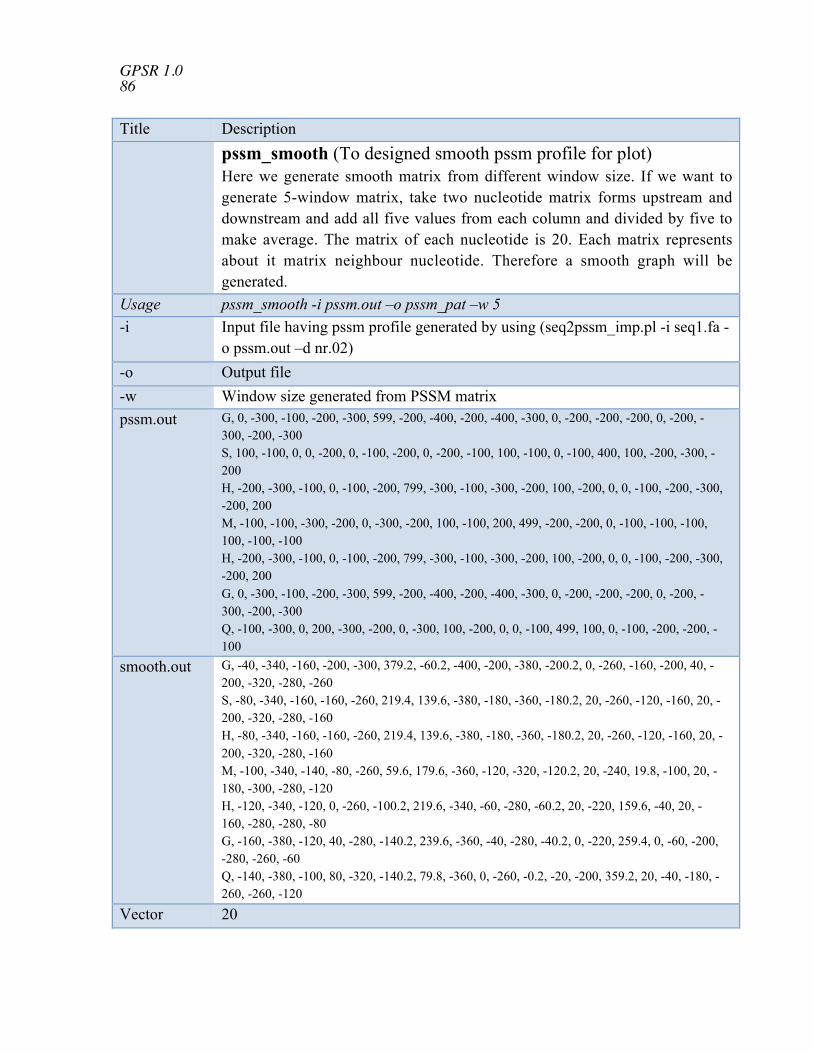
GPSR 1.0 86

Title Description

pssm_smooth (To designed smooth pssm profile for plot)Here we generate smooth matrix from different window size. If we want togenerate 5-window matrix, take two nucleotide matrix forms upstream anddownstream and add all five values from each column and divided by five tomake average. The matrix of each nucleotide is 20. Each matrix representsabout it matrix neighbour nucleotide. Therefore a smooth graph will begenerated.

Usage pssm_smooth -i pssm.out –o pssm_pat –w 5

-i Input file having pssm profile generated by using (seq2pssm_imp.pl -i seq1.fa -o pssm.out –d nr.02)

-o Output file

-w Window size generated from PSSM matrix

pssm.out G, 0, -300, -100, -200, -300, 599, -200, -400, -200, -400, -300, 0, -200, -200, -200, 0, -200, -300, -200, -300S, 100, -100, 0, 0, -200, 0, -100, -200, 0, -200, -100, 100, -100, 0, -100, 400, 100, -200, -300, -200H, -200, -300, -100, 0, -100, -200, 799, -300, -100, -300, -200, 100, -200, 0, 0, -100, -200, -300,-200, 200M, -100, -100, -300, -200, 0, -300, -200, 100, -100, 200, 499, -200, -200, 0, -100, -100, -100,100, -100, -100H, -200, -300, -100, 0, -100, -200, 799, -300, -100, -300, -200, 100, -200, 0, 0, -100, -200, -300,-200, 200G, 0, -300, -100, -200, -300, 599, -200, -400, -200, -400, -300, 0, -200, -200, -200, 0, -200, -300, -200, -300Q, -100, -300, 0, 200, -300, -200, 0, -300, 100, -200, 0, 0, -100, 499, 100, 0, -100, -200, -200, -100

smooth.out G, -40, -340, -160, -200, -300, 379.2, -60.2, -400, -200, -380, -200.2, 0, -260, -160, -200, 40, -200, -320, -280, -260S, -80, -340, -160, -160, -260, 219.4, 139.6, -380, -180, -360, -180.2, 20, -260, -120, -160, 20, -200, -320, -280, -160H, -80, -340, -160, -160, -260, 219.4, 139.6, -380, -180, -360, -180.2, 20, -260, -120, -160, 20, -200, -320, -280, -160M, -100, -340, -140, -80, -260, 59.6, 179.6, -360, -120, -320, -120.2, 20, -240, 19.8, -100, 20, -180, -300, -280, -120H, -120, -340, -120, 0, -260, -100.2, 219.6, -340, -60, -280, -60.2, 20, -220, 159.6, -40, 20, -160, -280, -280, -80G, -160, -380, -120, 40, -280, -140.2, 239.6, -360, -40, -280, -40.2, 0, -220, 259.4, 0, -60, -200,-280, -260, -60Q, -140, -380, -100, 80, -320, -140.2, 79.8, -360, 0, -260, -0.2, -20, -200, 359.2, 20, -40, -180, -260, -260, -120

Vector 20

GPSR 1.0 87

Title Description

seq2motif (To create motifs by sliding window of user definedlength)This program creates motif of defined length. Additional 'X' at the end ofsequence is added to make complete pattern. The binary pattern isgenerated using the motifs

Usage seq2motif -i seq1.fa -o motif.out -w 5-i Input file in single fasta format-o Output file-w Window size to create a pattern

seq1.fa >seq_1##GSHMHGQVDCSPGIWQLDCTHLEGK

motif_1.out >seq_1XXGSHXGSHMGSHMHSHMHGHMHGQMHGQVHGQVDGQVDCQVDCSVDCSPDCSPGCSPGISPGIWPGIWQGIWQLIWQLDWQLDCQLDCTLDCTHDCTHLCTHLETHLEGHLEGKLEGKXEGKXX

GPSR 1.0 88

Title Description

seq2motif _simple (To create motifs by sliding window of userdefined length)This program creates motif of defined length. This program is similar toseq2motif program but generates motifs without adding 'X' at the end.Binary pattern is generated using these motifs.

Usage seq2motif_simple -i seq1.fa -o motif_2.out -w 5

-i Input file in single fasta format-o Output file-w Window size to create a patternseq1.fa >seq_1##GSHMHGQVDCSPGIWQLDCTHLEGK

motif_2.out >seq_1GSHMHSHMHGHMHGQMHGQVHGQVDGQVDCQVDCSVDCSPDCSPGCSPGISPGIWPGIWQGIWQLIWQLDWQLDCQLDCTLDCTHDCTHLCTHLETHLEGHLEGK

GPSR 1.0 89

Title Description

motif2bin (To make binary input from the multifasta motif file)It generates binary input from the multifasta motif file of fixed length intocolumn format.

Usage motif2bin -i motif_1.out -o bin.out -x y-i Input in multifasta file (seq2motif.pl -i seq1.fa -o motif.out -w 5)

-o Output file-x If additional X is added in pattern then y (for yes), or n (for no)motif_1.out >seq_1

XXGSHXGSHMGSHMHSHMHGHMHGQMHGQVHGQVDGQVDCQVDCSVDCSPDCSPGCSPGISPGIWPGIWQGIWQLIWQLDWQLDCQLDCTLDCTHDCTHLCTHLETHLEGHLEGKLEGKXEGKXX

bin.out 0, 0, 0, 0, 0, 0, 0, 0, 0, 0, 0, 0, 0, 0, 0, 0, 0, 0, 0, 0, 1, 0, 0, 0, 0, 0, 0, 0, 0, 0, 0, 0, 0, 0, 0, 0,0, 0, 0, 0, 0, 1, 0, 0, 0, 0, 0, 1, 0, 0, 0, 0, 0, 0, 0, 0, 0, 0, 0, 0, 0, 0, 0, 0, 0, 0, 0, 0, 0, 0, 0, 0,0, 0, 0, 0, 0, 0, 1, 0, 0, 0, 0, 0, 0, 0, 0, 0, 0, 0, 1, 0, 0, 0, 0, 0, 0, 0, 0, 0, 0, 0, 0, 0, 00, 0, 0, 0, 0, 0, 0, 0, 0, 0, 0, 0, 0, 0, 0, 0, 0, 0, 0, 0, 1, 0, 0, 0, 0, 0, 1, 0, 0, 0, 0, 0, 0, 0, 0, 0,0,0, 0, 0, 0, 0,0, 0, 0, 0, 0, 0, 0, 0, 0, 0, 0, 0, 0, 0, 0, 1, 0, 0, 0, 0, 0, 0, 0, 0, 0, 0, 0, 1, 0, 0, 0,0, 0, 0, 0, 0, 0, 0, 0, 0, 0, 0, 0, 0, 0, 0, 0, 0, 0, 0, 0, 0, 1, 0, 0, 0, 0, 0, 0, 0, 0, 0, 0…………………………………………

Vector 20*window size (20*5=100)

GPSR 1.0 90

Title Description

blast similarity (To perform blast)Basic Local Alignment Search Tool, or BLAST, is an algorithm for comparingprimary biological sequence information, such as the amino-acid sequences ofdifferent proteins or the nucleotides of DNA sequences. A BLAST search enables aresearcher to compare a query sequence with a library or database of sequences,and identify library sequences that resemble the query sequence above a certainthreshold. For example, following the discovery of a previously unknown protein inthe mouse, a scientist will typically perform a BLAST search of the proteindatabase (nr) to see if humans carry a similar protein; BLAST will identifysequences in the previously known database that resemble the mouse protein basedon similarity of sequence.

Usage blast_similarity -i fasta -d nr -j 3 -e 1 –o blast.out

-i Input file of Fasta format-o Output result-d Database used blast

-j Number of Iteration-e Cut off Evaluefasta >amla_1

ASDATAYAACVAYANMANNNAMAKLAWQAPTCAGYAAKTGCVQRATRQOPKALVNAASDREW>amla_2ACDEFGHIKLMNPQRSTVWMRNRGFGRRELLVAMAMLVSVTGCARHASGARPASTTLPAGADLADRFAELERRYDARLG

blast.out >amla_1 Zero Zero>amla_2 ref|NP_216584.1| blaC [Mycobacterium tuberculosis H37Rv] >gi|158... 2e-27

GPSR 1.0 91

Stand-alone Programs

GPSR 1.0 92

Installation of GPSR 1.0 package locally

GPSR 1.0: This package developed mainly for UNIX machines. It can bedownloaded from www.imtech.res.in/raghava/gpsr/

Prerequisite softwares for GPSR 1.0 package

SVMlight: freely available software (academic). It can be downloaded (old:version 5.0 and new 6.1) from http://download.joachims.org/svm_light/current/svm_light.tar.gz.

HMMER: freely available software (academic). User can download the sourcecode from ftp://ftp.genetics.wustl.edu/pub/eddy/hmmer/

MEME/MAST: freely available software (academic). User can download thesource code from http://meme.nbcr.net/meme4_1/meme-download.html

BLAST: freely available software (academic). User can download thesource code from http://www.ncbi.nlm.nih.gov/BLAST/download.shtml

cdk.jar: freely available software (academic). User can download thesource code from http://sourceforge.net/projects/cdk/

To uncompress gpsr.tar.gz, execute the following command$ tar -zxf gpsr.tar.gz

To install package$ cd gpsr$ perl install.pl

During installation it will ask for the path of required softwares like Perl, BLAST,SVM old (version 5.0), SVM New (version 6.1), MEME/MAST etc. The entireprogram will be installed in the bin folder.

To update package $ perl update.plOnce you have installed the gpsr package and wish to update the package or

GPSR 1.0 93

change/add the path of any software later, you may run update.pl instead ofinstall.pl.

ESLPred2

Application:ESLpred2 trained using organism specific and generalized datasets can be used for theprediction of eukaryotic subcellular localizations. The webserver is available athttp://www.imtech.res.in/raghava/eslpred2/

Introduction:In this post genomic era, functional annotation and characterization of nearly millions ofraw protein sequences, erupted by incredible sequencing projects, are some of theinescapable challenges that has been baffling the scientific community in order to bridgethe mounting gap between number of unknown and annotated proteins. This crisis entailsthe development of computational methods that would help in predicting functions ofproteins expeditiously as well as economically. One of the fundamental and popularindirect strategies for assigning function is the identification of subcellular compartmentsof proteins as knowledge about localization can provide important indications aboutprotein functions. After PSORT the first method developed to predict the subcellularlocalizations, ample of novice, improved, generalized and organism specific predictionmethods have been developed for predicting subcellular locations of eukaryotic andprokaryotic proteins, namely, NNPSL, PSORTB, FKNN, TargetP, SubLoc, SignalP,CELLO, LOCnet, PSLpred, HSLPred, PLOC, Mutiloc, Proteome Analyst, LOCtree,TSSub, BaCelLo and Esub8 using different datasets and protein input features. In 2004,our group has combined the information of similarity search with sequence compositionbased attributes (ESLPred) and achieved accuracy up to 88%. In ESLPred2, a systematicapproach has been taken to improve the prediction quality of eukaryotic subcellularlocalizations using PSI-BLAST generated PSSM profiles along with compositionalattributes and similarity search based information for the training of SVM. The presentmethod has achieved a highest success rate for the prediction of localizations with goodoverall and average accuracy, and hence, compliments the existing subcellularlocalization prediction methods.

Datasets:ESLPred2 was trained using the latest dataset, which was earlier used for developingBaCelLo method. The dataset was retrieved from SWISSPROT version 48.0 and dividedinto three subsets on the basis of kingdoms- animal with 2597 sequences; fungi with 1198sequences and 491 sequences were from plant. The major attraction of this dataset wasthe stringent cut-off value of 30% used to reduce the similarity between sequences. The

GPSR 1.0 94

first two datasets covered 4 major localizations such as cytoplasm, mitochondria, nuclear,and extracellular, whereas, plant dataset included chloroplast class along with four majorlocalizations. In addition, RH2427 dataset was also used to train a generalized model forprediction of eukaryotic proteins subcellular localizations.

ResultsThe hybrid approach based module which incorporated similarity search basedinformation with amino acid composition of a single sequence (whole and N-terminal)and profiles for RH2427 dataset attained an overall accuracy to ~94% and averageaccuracy for four localizations to 93.1%. Using this hybrid approach, cytoplasmic,mitochondrial, nuclear, and extracellular proteins has been predicted with 89.6%, 90.7%,96.4%, and 95.7% of accuracies respectively. Additionally, ESLpred2 has also been ableto attain best accuracies of 80.8,75.9%, and 76.6% for kingdom specific animal, fungiand plant proteins respectively, which is the best accuracy reported till date for the samedataset. Hence, ESLpred2 provides more crucial and promising features for prediction ofeukaryotic subcellular localizations coupled with kingdom specific prediction SVMmodels. An interesting feature of the present method is the hybrid of different proteinfeatures, such as composition of PSSM profile, whole and N-terminal composition ofsequence and similarity search based results, which supported the assignment of thesubcellular localization of proteins more reliably and with high accuracy irrespective ofredundancy in the training datasets. The present method is able to complement allexisting subcellular location prediction methods.

Usage of standalone versionperl eslpred2 -i <seq_file> -m <method> -k <organism> -o <output_file>

Seq_file is a file containing protein sequences (single or multiple) in fasta format. Method defines the 3 modules for the prediction of subcellular localizations such

asa) Amino acid compositions (1);b) PSSM (2)c) Hybrid module for AAC, PSSM and PSI-BLAST based similarity (3).

Organism defines the models based on training dataset such asa) A for Animal dataset;b) F for Fungi dataset;c) P for Plant dataset.d) G for generalized dataset (RH2427)

Output_file defines the name of output file for storing results

Publication:

GPSR 1.0 95

Garg A and Raghava GPS (2008) ESLpred2: Improved method for predicting subcellularlocalization of eukaryotic proteins. BMC Bioinformatics, 9:503.

GPSR 1.0 96

ESLPred

ApplicationESLPred is a SVM-based method for the prediction of subcellular localization ofe u k a r y o t i c p r o t e i n s . T h e w e b s e r v e r i s a v a i l a b l e a thttp://www.imtech.res.in/raghava/eslpred/

IntroductionLarge-scale genome sequencing projects make interpretation of genomic sequence dataincreasingly important, so does the need to functionally annotate this data. Thedetermination of subcellular localization of a protein can provide important clues toelucidate the function of the protein. Therefore, prediction of subcellular localization ofproteins is an important step in understanding the biochemical function of proteins. In thepast, various methods have been developed to predict the subcellular location of proteinsusing different approaches. The similarity search in which a sequence is searched againstan experimentally annotated database, is a technique commonly used to assign functionto a protein, including its subcellular location. This approach fails in the absence ofsignificant similarity between query and target protein sequences. Another way to predictsubcellular localization of proteins is to identify sequence motifs such as signal peptide ornuclear localization signal. The major limitation of motif-based methods is that allproteins residing in a compartment do not have universal motifs.To overcome these limitations, in the past numerous studies have been carried out topredict subcellular localization based on the features of protein sequence. The subcellularlocalization prediction methods are based either on recognition of N-terminal sortingsignals or on the composition of amino acids. In ESLPred, a systematic attempt has beenmade to achieve higher prediction accuracy for subcellular localization of eukaryoticproteins from their different features. The SVM modules were developed based on thefollowing features of a protein: (i) amino acid composition (commonly used in theliterature for classification of proteins), (ii) overall physico-chemical properties (e.g.hydrophobicity, hydrophilicity, polarity) and (iii) dipeptide compositions (e.g. ala–ala,ala–leu, val–ser). In addition, a similarity search based module, EuPSI-BLAST, was alsoconstructed using PSI-BLAST to predict the localization of a protein. Finally, a hybridSVM module was developed using all three features of proteins mentioned above andprediction results of EuPSI-BLAST.

DatasetsThe dataset used in devloping ESLPred was also used in the development of SubLoc andNNPSL. This dataset was generated from version 33.0 of SWISS-PROT by Reinhardtand Hubbard (RH2427). The dataset consisted of complete and non-redundant proteins

GPSR 1.0 97

with less than 90% sequence identity whose subcellular localization is experimentallydetermined. This dataset consisted of a total of 2427 eukaryotic proteins (1097 nuclear,684 cytoplasmic, 321 mitochondrial and 325 extracellular proteins).

ResultsSupport vector machine (SVM) has been used to predict the subcellular location ofeukaryotic proteins from their different features such as amino acid composition,dipeptide composition and physico-chemical properties. The SVM module based ondipeptide composition performed better than the SVM modules based on amino acidcomposition or physico-chemical properties. In addition, PSI-BLAST was also used tosearch the query sequence against the dataset of proteins (experimentally annotatedproteins) to predict its subcellular location. In order to improve the prediction accuracy,we developed a hybrid module using all features of a protein, which consisted of an inputvector of 458 dimensions (400 dipeptide compositions, 33 properties, 20 amino acidcompositions of the protein and 5 from PSI-BLAST output). Using this hybrid approach,the prediction accuracies of nuclear, cytoplasmic, mitochondrial and extracellularproteins reached 95.3, 85.2, 68.2 and 88.9%, respectively. The overall predictionaccuracy of SVM modules based on amino acid composition, physico-chemicalproperties, dipeptide composition and the hybrid approach was 78.1, 77.8, 82.9 and88.0%, respectively. The accuracy of all the modules was evaluated using a 5-fold cross-validation technique. Assigning a reliability index (reliability index 3), 73.5% ofprediction can be made with an accuracy of 96.4%.

Usage of standalone versionperl eslpred -i <seq_file> -m <method> -o <output_file>

Seq_file is a file containing protein sequences (single or multiple) in fasta format. Method defines the 5 trained SVM modules for the prediction of subcellular

localizations such asa) Amino acid compositions (1);b) Overall physico-chemical properties (2);c) Dipeptide compositions (3);d) PSI-BLAST similarity based (4);e) Hybrid module (5).

Output_file defines the name of output file for storing results

PublicationBhasin M and Raghava GPS (2004) ESLpred: SVM Based Method for SubcellularLocalization of Eukaryotic Proteins using Dipeptide Composition and PSI-BLAST.Nucleic Acids Research 32:W414-9.

GPSR 1.0 98

HSLPred

ApplicationHSLPred is a SVM-based method for the prediction of subcellular localizations of humanproteins. The webserver is available at http://www.imtech.res.in/raghava/hslpred/

IntroductionThe successful completion of a human genome project has yielded huge amount ofsequence data. Analysis of this data to extract the biological information can haveprofound implications on biomedical research. Therefore, mining of biologicalinformation or functional annotation of piled up sequence data is a major challenge to themodern scientific community. Determination of functions of all of these proteins usingexperimental approaches is a difficult and time-consuming task. Traditionally, thesimilarity search-based tool has been used for functional annotations of proteins. Thisapproach fails when unknown query protein does not have significant homology toproteins of known functions. The functions of the proteins are closely related to itscellular attributes, such as subcellular localization and its association with the lipidbilayer (subcellular localization) hence, the related proteins must be localized in the samecellular compartment to cooperate toward a common function. In addition, informationon the localization of proteins with known function may provide insight about itsinvolvement in specific metabolic pathways. Therefore, an attempt has been made topredict subcellular localization of proteins to elucidate the function. Several methodshave been devised earlier to predict the subcellular localization of the eukaryotic andprokaryotic proteins using different approaches and data sets. To the best of ourknowledge, there is no method for the prediction of subcellular localization of humanproteins. Availability of sequence data of human genes in recent years demands a reliableand accurate method for prediction of subcellular localization of human proteins.HSLpred is based on different features of the proteins such as amino acid and dipeptidecomposition of proteins. In addition, a similarity search-based module, HuPSI-BLAST,has also been developed, using PSI-BLAST to predict the localization of human proteins.Further, SVM module "hybrid1" has been developed using amino acid composition,traditional dipeptide composition, and results of PSI-BLAST prediction. The SVMmodules based on higher order dipeptide compositions (i + 2, i + 3, and i + 4) andcombinations of various feature-based modules have also been constructed. In addition,the performance of HSLPred has also been assessed on various mammalian andnonmammalian genomes and on an independent data set. It was observed that thismethod can predict the subcellular localization of human proteins and proteins fromrelated genomes with high accuracy. In other words, our method can also be used for theprediction of subcellular localization of mammalian proteins.

GPSR 1.0 99

DatasetsThe dataset of human proteins used to devlop HSLpred was extracted from specialrelease of SWISSPROT database. Final non-redundant data set consisted of a total of3532 human proteins (840 cytoplasmic, 315 mitochondrial, 858 nuclear, 1519 plasmamembrane). The dataset is available at www.imtech.res.in/raghava/hslpred.

ResultsSVM based modules for predicting subcellular localization using traditional amino acidand dipeptide (i + 1) composition achieved overall accuracy of 76.6 and 77.8%,respectively. PSI-BLAST, when carried out using a similarity-based search against anonredundant data base of experimentally annotated proteins, yielded 73.3% accuracy.To gain further insight, a hybrid module (hybrid1) was developed based on amino acidcomposition, dipeptide composition, and similarity information and attained betteraccuracy of 84.9%. In addition, SVM modules based on a different higher order dipeptidei.e. i + 2, i + 3, and i + 4 were also constructed for the prediction of subcellularlocalization of human proteins, and overall accuracy of 79.7, 77.5, and 77.1% wasaccomplished, respectively. Furthermore, another SVM module hybrid2 was developedusing traditional dipeptide (i + 1) and higher order dipeptide (i + 2, i + 3, and i + 4)compositions, which gave an overall accuracy of 81.3%. We also developed SVMmodule hybrid3 (final) based on amino acid composition, traditional and higher orderdipeptide compositions, and PSI-BLAST output and achieved an overall accuracy of84.4%.

Usage of standalone versionperl hslpred -i <seq_file> -m <method> -o <output_file>

Seq_file is a file containing protein sequences (single or multiple) in fasta format. Method defines the 4 trained SVM modules for the prediction of subcellular

localizations such asa) Amino acid compositions (1);b) Dipeptide compositions (2);c) PSI-BLAST similarity based (3);d) Hybrid module (a+b+c+d) (4).

Output_file defines the name of output file for storing resultsPublicationGarg A, Bhasin M and Raghava GP (2005) SVM-based method for subcellularlocalization of human proteins using amino acid compositions, their order and similaritysearch. J Biol Chem 280:14427-32.

GPSR 1.0 100

GPSR 1.0 101

PSLpred

ApplicationPSLpred is a SVM-based method for the prediction of subcellular localizations ofp r o k a r y o t i c p r o t e i n s . T h e w e b s e r v e r i s a v a i l a b l e a thttp://www.imtech.res.in/raghva/pslpred/

IntroductionProkaryotes are the causative agent of most of the deadly disease and widespread ofepidemics, hence, biologists are paying much attention for the functional annotation ofprokaryotic proteins. This may further guide the determination of virulence factors aswell as new pattern of resistance for antiobiotic agents in pathogenic bacteria. Hence,prediction of protein subcellular localization (an alternative to functional annotation) ofgram-negative bacteria would be very useful in the field of molecular biology, cellbiology, pharmacology, and medical science. A number of methods such as PSORT I,PSORT-B and NNPSL have been developed for predicting subcellular localization ofbacterial proteins based on different datasets and computational techniques. Theaccuracies reported by these methods vary between 60 and 81%. Recently, a supportvector machines (SVM) based method, CELLO trained using n-peptide compositions hasbeen developed for predicting subcellular localization of bacterial proteins. This methodhas achieved an overall accuracy of 89% that is better than existing methods forsubcellular localizationof prokaryotic proteins. Despite the overall improved performance, CELLO predictsextracellular proteins with a fair accuracy of 78.9%, proteins that may representimportant virulence factors in pathogenic microorganisms. PSLpred a SVM basedmethod has been devloped for the prediction of subcellular localization of prokaryoticproteins using input features such as amino acid and dipeptide composition, physico-chemical properties along with similarity search based results.

DatasetsThe data set used in the present study is the same as that used for developing the methodsCELLO and PSORT-B, respectively. This data set has been generatedfrom SWISSPROTrelease 40.29 and consisted of a total of 1443 proteins belonging to different subcellularlocalizations. We have excluded 141 proteins residing in more than one subcellularlocations and used the remaining 1302 proteins (248 cytoplasmic, 268 inner membrane,244 periplasmic, 352 outer membrane and 190 extracellular) for the development ofPSLpred.

GPSR 1.0 102

ResultsPSLpred is a hybrid approach-based method that integrates PSI-BLAST and three SVMmodules based on compositions of residues, dipeptides and physico-chemical propertiesand predicts the subcellular localization of gram-negative bacterial proteins with anoverall accuracy of 91.2%. The prediction accuracies of 90.7, 86.8, 90.3, 95.2 and 90.6%were attained for cytoplasmic, extracellular, inner-membrane, outer-membrane andperiplasmic proteins, respectively. Furthermore, PSLpred was able to predict 74% ofsequences with an average prediction accuracy of 98% at RI = 5. The performance of thehybrid module was compared with methods such as CELLO, PSORT-B, which were alsodeveloped from the same data set. It has been observed that overall performance of thehybrid module is nearly 2% higher than CELLO and 16% higher than that of PSORT-B.Hence PSLpred is more accurate for the subcellular localization of prokaryotic proteins.

Usage of standalone versionperl pslpred -i <seq_file> -m <method> -o <output_file>

Seq_file is a file containing protein sequences (single or multiple) in fasta format. Method defines the 5 trained SVM modules for the prediction of subcellular

localizations such asa) Amino acid compositions (1);b) Physico-chemical properties (2);c) Dipeptide compositions (3);d) PSI-BLAST similarity based (4);e) Hybrid module (5).

Output_file defines the name of output file for storing results

PublicationBhasin M. Garg A and Raghava GPS (2005) PSLpred: prediction of subcellularlocalization of bacterial proteins. Bioinformatics 21(10):2522-4.

GPSR 1.0 103

SRTPred

ApplicationSRTPred is a SVM-based method for the classification of protein sequence as secretoryor non-secre to ry p ro te in . The webserver i s ava i lab le a thttp://www.imtech.res.in/raghava/srtpred/

IntroductionProtein secretion is a universal process which occurs in all organisms and has tremendousimportance to biological research. In case of pathogenic microorganisms, secretorypathways deliver virulence factors to their sites of action, soluble extracellular enzymesinto the surrounding medium, or for specifically targeting proteins to the host cell. Inseveral instances, protein secretion pathways are similar to those involved in assembly ofbacterial appendages. Further, several secretory proteins has been identified as a majortarget protein for the development of drugs. Hence, development of automatic method forthe prediction of secretory proteins would be a help for the studies aim towardsdeciphering secretory pathways and also lead to the identification of novel drug targetswith greater value for biomedical research.Until now, many methods have been developed for the classification and prediction ofsubcellular localizations of proteins based on signal peptide (SPs), mainly SignalP andpTarget. TargetP is a neural-network based method that discriminates between proteinsdestined for the mitochondrion, the chloroplast, the secretory pathways and otherlocalizations with a success rate of 85.3% (overall) and sensitivity of 0.96 for non-plantsecretory proteins. Whereas, neural network based method, SignalP (version 3.0) methodhas been able to achieve high sensitivity of 0.99 and overall accuracy of 0.93 foreukaryotic signal peptide discrimination. Though achieving higher prediction accuracyfor classical secreted proteins, these methods, unfortunately fail during the prediction ofproteins without SP. Hence, non-classical secreted proteins also demand automatedmethod for the prediction. Recently, a webserver SecretomeP has been developed topredict non-classical secreted proteins, based on an idea that extracellular proteins sharecertain features regardless of the pathway used to secrete them. It is a neural networkbased method that has used several features of protein such as number of atoms,positively charged residues, propeptide cleavage site, protein sorting, low complexityregions, and transmembrane helices as an input to train network. Despite consideringlarge number of protein features, the method has achieved a false positive prediction thatis less than 5% at a low sensitivity value of 40%. Till date, there is not any methodavailable that can predict secretory proteins, irrespective of pathways/SPs, with betteraccuracy. SRTPred is an automated method that can predict secretory proteins(irrespective of N-terminal SP) based on different features of whole protein sequence.

GPSR 1.0 104

DatasetThe data set used in the present study, consisted of 6975 mammalian protein sequences.Out of which 3321 sequences were extracellular proteins secreted via classical and non-classical pathways (positive examples), whereas the remaining 3654 proteins wereannotated as cytoplasmic and/or the nuclear (negative examples). Previously, the samedataset was used to develop a method SecretomeP and available publicly athttp,//www.cbs.dtu.dk/services/SecretomeP-1.0/datasets.php. The sequences wereextracted from Swiss-Prot database on the basis of subcellular localization annotations inthe comment block.

ResultsSRTpred is a systematic attempt to predict secretory proteins irrespective of presence orabsence of N-terminal signal peptides (also known as classical and non-classical secretedproteins respectively), using machine-learning techniques; artificial neural network(ANN) and support vector machine (SVM). We trained and tested our methods on adataset of 3321 secretory and 3654 non-secretory mammalian proteins using five-foldcross-validation technique. First, ANN-based modules have been developed forpredicting secretory proteins using 33 physico-chemical properties, amino acidcomposition and dipeptide composition and achieved accuracies of 73.1%, 76.1% and77.1%, respectively. Similarly, SVM-based modules using 33 physico-chemicalproperties, amino acid, and dipeptide composition have been able to achieve accuracies77.4%, 79.4% and 79.9%, respectively. In addition, BLAST and PSI-BLAST modulesdesigned for predicting secretory proteins based on similarity search achieved 23.4% and26.9% accuracy, respectively. Finally, we developed a hybrid-approach by integratingamino acid and dipeptide composition based SVM modules and PSI-BLAST module thatincreased the accuracy to 83.2%, which is significantly better than individual modules.We also achieved high sensitivity of 60.4% with low value of 5% false positivepredictions using hybrid module.

Usage of standalone versionperl srtpred -i <seq_file> -m <method> -t <threshold value) -o <output_file>

Seq_file is a file containing protein sequences (single or multiple) in fasta format. Method defines the 5 trained SVM modules for the prediction of secretory

proteins such asa) Amino acid compositions (1);b) Properties based (2);c) Dipeptide compositions (3);d) PSI-BLAST similarity based (4);e) Hybrid module of a+c+d (5).

GPSR 1.0 105

Threshold_value defines the selection of threshold value in the range of -1.5 to1.5

Output_file defines the name of output file for storing results

PublicationGarg A and Raghava GPS (2008) A machine learning based method for the prediction ofsecretory proteins using amino acid composition, their order and similarity-search. InSilico Biology 8:129-40.

GPSR 1.0 106

OxyPred

ApplicationOxyPred is a SVM based method to predict the Oxygen Binding Proteins such asErythrocruorin, Hemoglobin, Myoglobin, Hemerithrin, Leghemoglobin and Hemocyanin.The webserver is available at http://www.imtech.res.in/raghava/oxypred/

IntroductionOxygen-binding proteins are widely present in eukaryotes ranging from non-vertebratesto humans. Moreover, these proteins have also been reported to be present in manyprokaryotes and protozoans. The occurrence of oxygen-binding proteins in all kingdomsof organisms, though not in all organisms, shows their biological importance. Extensivestudies on oxygen-binding proteins have categorized them into six different broad types,including ery-throcruorin, hemerythrin, hemocyanin, hemoglobin, leghemoglobin, andmyoglobin, each has its own functional characteristics and structure with unique oxygen-binding capacity. These oxygen-binding proteins are crucial for the survival of any livingorganism. With the advancement in sequencing technology, the size of protein sequencedatabases is growing at an exponential rate. Thus it is much needed to developbioinformatics methods for functional annotation of proteins, particularly for identifyingoxygen-binding proteins. We have developed a reliable SVM-based method forpredicting and classifying oxygen-binding proteins using different residue compositions.

DatasetThe sequences of oxygen-binding proteins and non-oxygen-binding proteins from theSwiss-Prot database (http://www.expasy.org/sprot/). In order to obtain a high-qualitydataset, we removed all those proteins annotated as “fragments", “isoforms", “potentials",“similarity", or “probables" and created a non-redundant dataset where no two proteinshave a similarity more than 90% using PROSET software. Our final dataset consisted of672 oxygen-binding proteins and 700 non-oxygen binding proteins. These 672 oxygen-binding proteins were then classified into six different classes, consisting of 20erythrocruorin, 31 hemerythrin, 77 hemocyanin, 486 hemoglobin, 13 heghemoglobin, and45 myoglobin proteins.

ResultsSVM modules were developed using amino acid composition and dipeptide compositionfor predicting oxygen-binding proteins and achieved maximum accuracy of 85.5% and87.8%, respectively. Secondly, SVM module was developed based on amino acidcomposition, classifying the predicted oxygen-binding proteins into six classes withaccuracy of 95.8%, 97.5%, 97.5%, 96.9%, 99.4%, and 96.0% for erythrocruorin,

GPSR 1.0 107

hemerythrin, hemocyanin, hemoglobin, leghemoglobin, and myoglobin proteins,respectively. Finally, a module was developed using dipeptide composition forclassifying the oxygen-binding proteins, and achieved maximum accuracy of 96.1%,98.7%, 98.7%,85.6%, 99.6%, and 93.3% for the above six classes, respectively.

Usage of standalone versionperl oxypred -i <seq_file> -m <method> -o <output_file>

Seq_file is a file containing protein sequences (single or multiple) in fasta format. Method defines the 2 trained SVM modules for the prediction such as

a) Amino acid compositions (1);b) Dipeptide compositions (2);

Output_file defines the name of output file for storing results

PublicationMuthukrishnan S, Garg A and Raghava GPS (2007) OxyPred: Prediction andClassification of Oxygen-Binding Proteins. Genomics, Proteomics & Bioinformatics5:250-2

GPSR 1.0 108

DPROT

ApplicationDPROT is a SVM based method to predict disordered proteins using evolutionaryinformation. The webserver is available at http://www.imtech.res.in/raghava/dprot/

IntroductionThe knowledge of three dimensional (3D) structure of a protein is essential to deduce itsbiological function. Since, prediction of secondary structure is an intermediate step instructure determination, hence, in the past number of secondary and super secondarystructure prediction methods have been developed by our. However, past few years haveseen a growing interest in structural studies of proteins, focusing comprehensively on thestudy of proteins which are structurally disordered, often, known as disordered proteins.These proteins have been gaining high attention from biologists, since their involvementin various physiological disorders which could be protein deposition diseases such asAlzheimer's and Parkinson's diseases became evident. From the structure point of view, adisordered protein, or disordered regions, are those lacking a specific tertiary structureand is composed of an ensemble of conformations, usually with distinct and dynamic _and _. These proteins in their purified state at neutral pH, either have been shownexperimentally or are predicted to lack ordered structure. Existence of disorder isdetermined by overall protein dynamics rather than by local secondary structure. Theseproteins are also referred as “natively unfolded” or “intrinsically unstructured”.Several predictors have been developed in the past for instance PONDR (Jones et al.2003), DISOPRED2 (Ward et al. 2004), GlobPlot (Linding et al. 2003), DISEMBL(Linding et al. 2003), FoldIndex (Sussman et al. 2005) and RONN (Yang et al. 2005) etc.for predicting disorder proteins/regions. All these predictors exploit various attributes ofthe protein sequence such as amino acid compositions, flexibility, charge, hydropaths,PSIBLAST profiles, propensities for secondary structure and random coils etc. On theother hand, IUPRED (Dosztanyi et al. 2005) which is based on inter-residue interactions,predicts regions that lack a well defined 3D structure under native conditions, whilst,FoldUnfold (Galzitskaya et al. 2006), predicts disordered regions by estimating thenumber of contacts of the whole protein. Recently, a predictor POODLE has beendeveloped (Shimizu et al. 2007), which can predict disordered proteins with a highsensitivity value of 72.3% and an accuracy of 97.7%. POODLE is based on joachims’spectral graph transducer (SGT), which is a binary classification based on semi-supervised learning. Despite gaining such higher prediction accuracy, the method seemsto be insensitive for the set partially disordered proteins. This insensitivity might be dueto the utilization of single protein feature namely amino acid composition for prediction.The present study has been undertaken to further improve the prediction performance for

GPSR 1.0 109

classifying ordered and disordered proteins with an introduction to new input feature likesecondary structure composition, along with conventionally used protein features such asamino acid composition, dipeptide composition, and Position Specific Scoring Matrices(PSSM) composition. However, best performance was observed for PSSM based modulecapturing the multiple sequence alignment information for the prediction of disorderedproteins, hence, the module has been implemented on web server and standalone version.

DatasetA representative dataset consisting of 608 proteins: 526 ordered and 82 disorderedproteins. The same dataset was earlier used to develop the POODLE web server. Its rawdataset retrieved from Disprot (version 3.3), was later on processed by following anintensive protocol. Additionally, a data set of 417 partially disordered proteins was alsoused for independent testing.

ResultsThe association of structurally disordered proteins with a number of diseases hasengendered an enormous interest and hence, demands a prediction method which wouldcomprehend their study at molecular level expeditiously. DPROT is computationalmethod for prediction of disordered proteins using sequence and profile compositions asinput features for the training of SVM models. First, we developed the amino acid anddipeptide composition based SVM modules, which were able to yield sensitivity of 75.6and 73.2% along with MCC values of 0.75 and 0.60 respectively. In addition, the use ofpredicted secondary structure content (coil, sheet and helices) in the form of compositionvalues attained 76.8% and 0.77 of sensitivity and MCC values. Finally, training of SVMmodels using evolutionary information hidden in multiple sequence alignment profileimproved the prediction performance by achieving sensitivity value of 78% and MCC of0.78. Furthermore, the same SVM module when evaluated on an independent dataset ofpartially disordered proteins provided 86.6% of correct predictions.

Usage of standalone versionperl dprot -i <seq_file> -t <threshold value) -o <output_file>

Seq_file is a file containing protein sequences (single or multiple) in fasta format. Threshold_value defines the selection of threshold value in the rangeof -1.5 to

1.5 Output_file defines the name of output file for storing results

PublicationSethi D, Garg A and Raghava GPS (2008) DPROT: Prediction of Disordered Proteinsusing Evolutionary Information. Amino Acids 35:599-605.

GPSR 1.0 110

NRpred

ApplicationNRpred is a SVM based tool for the classification of nuclear receptors on the basis ofamino acid composition or dipeptide composition. The webserver is available athttp://www.imtech.res.in/raghava/nrpred/

IntroductionThe recognition of nuclear receptors is crucial because many of them are potential drugtargets for developing therapeutic strategies for diseases like breast cancer and diabetes.Nuclear receptors are one of the most abundant classes of transcriptional regulators,which regulate diverse functions during reproduction, metabolism and development.Nuclear receptors function as ligand activated transcriptional factors, providing a directlink between signaling molecules that control these processes and transcriptionalresponses. Besides this, nuclear receptors share a common structural organization. Allnuclear receptors consist of six distinct regions or domians: N- and C- terminal highlyvariable regions (A/B & F domains) that contain one or more transactivation regions, acentral well conserved DNA binding domain (C), a non conserved hinge region (D) thatcontains Nuclear Localization Signal (NLS) and a moderately conserved ligand bindingdomain (E) (4). The DNA binding domain (C region) of nuclear receptors consists of twozinc fingers, which act as a signature for this superfamily. The presence of these zincfingers facilitate the recognition of nuclear receptors from genome sequence using simplesimilarity based search tools like BLAST and FASTA . On the other hand, the majorlimitation of these search tools is that they are not able to classify the subfamilies ofnuclear receptors. The nuclear receptors have been classified to seven subfamilies, whichinclude thyroid and estrogen hormone like receptor according to nucleaRDB database.However, classification of these subfamilies is difficult by using the phylogeny orBLAST based tools due to scarcity of data for some subfamilies. Thus, there is a crucialneed for methods to enable automated assignment of nuclear receptor subfamilies. In thisreport, we have made an attempt to develop a method for recognizing the subfamilies ofnuclear receptors. We are able to design a method for recognizing the four subfamilies ofnuclear receptors: Thyroid hormone like (TR,RAR, ROR), HNF4-like (HNF4, RXR,TLL, Coup, USP), Estrogen like (ER, ERR, GR, MR, PR,AR) and Fushi tarazu-F1 like (SFI, FTF, FTZ-F1). Sequences for the other threesubfamilies are not available in significant number (less than 10). The classification ofnuclear receptors to various subfamilies was done on the basis of amino acid compositionand dipeptide composition. The amino acid and dipeptide composition are simplisticapproaches to produce patterns of fixed length from the protein sequences of varyinglength. In the past, the amino acid composition has been used to predict the domains

GPSR 1.0 111

structural class and subcellular localization of proteins. The dipeptide composition is alsowidely used to encapsulate the global information and giving a fixed pattern length of400. In the past, dipeptide composition has been used for the prediction of subcellularlocalization of proteins and for fold recognition. In this study, Support Vector Machines(SVM) was applied to classify nuclear receptors.

DatasetThe data for four subfamilies of nuclear receptors was obtained from nucleaRDBdatabase available at http://www.receptors.org/NR/. All the entries, which were notmarked as fragments, were extracted from the database by text parsing method. Theinitial dataset had 577 sequences belonging to four subfamilies of nuclear receptors.Redundancy was reduced so that no sequence had >=90% sequence identity with anyother sequence in the data set, using PROSET software. The final dataset contains 282sequences belonging to different subfamilies of nuclear receptors.

ResultsThe performance of all classifiers was evaluated using 5-fold cross validation test. It wasfound that different subfamilies of nuclear receptors were quite closely correlated interms of amino acid composition as well as dipeptide composition. The overall accuracyof amino acid composition and dipeptide composition based classifiers were 82.6% and97.5%, respectively. Therefore, our results proven that different subfamilies of nuclearreceptors are predictable with considerable accuracy using amino acid or dipeptidecomposition.

Usage of standalone versionperl nrpred -i <seq_file> -m <method> -o <output_file>

Seq_file is a file containing protein sequences (single or multiple) in fasta format. Method defines the 2 trained SVM modules for the prediction such as

a) Amino acid compositions (1);b) Dipeptide compositions (2);

Output_file defines the name of output file for storing results

PublicationBhasin M and Raghava GPS (2004) Classification of nuclear receptors based on aminoacid composition and dipeptide composition. J Biol Chem 279:23262-6

GPSR 1.0 112

PLPredApplicationPLPred is a SVM based method to predict and classify plastids. The webserver isavailable at http://www.imtech.res.in/raghava/plpred/

IntroductionPlastids are characteristic plant cell organelles that perform essential biosynthetic andmetabolic functions. These include photosynthetic carbon fixation, and the synthesis ofamino acids, fatty acids, starch and secondary metabolites such as pigments. On the basisof their structure, pigment composition (colour), metabolism and function, plastids areclassified as chloroplasts in photosynthetically active tissues, chromoplasts in fruits andpetals, amyloplasts in roots, etioplasts in dark-grown seedlings and elaioplasts that arefound in the seed endosperm. Although plastids are of significant biological interest, ourcurrent understanding of the metabolite functions and capacities of different plastid typesis still limited. However, Proteomics is a powerful approach to map the complete set ofplastid proteins and to infer plastid-type specific metabolite functions, only a fewproteomic approaches have been reported. Besides time consuming, the experimentalapproaches face several other constraints; for example, the chloroplast proteome analysisis nearing saturation because the detection of new proteins is constrained by highlyabundant photosynthetic proteins that dominate the proteome of photosynthetically activechloroplasts. To circumvent these constraints and to increase proteome coverage, thedevelopment of highly efficient computational prediction tools is another complementaryapproach to provide useful global information about the possible evolution of the plastidproteome. PLpred is an attempt in this direction which is a Support Vector Machine(SVM) based two-phase prediction tool for identifying as well as classifying the plastidproteins.Various features of a protein sequence viz. Amino acid composition, Dipeptidecomposition and Split Amino Acid Composition (SAAC) were exploited in thedevelopment of this prediction method. Secondly, the similarity search-based PSI-BLAST module was also developed. In addition, N-terminal and C-terminal amino acidcomposition based SVM modules as well as the Hybrid-based classifiers were alsodeveloped in order to encapsulate more comprehensive information from a proteinsequence. Conclusively, the best modules were selected and made available on this serverfor classification of plastid proteins.

DatasetTo infer various plastid-type specific functions, only a few proteomic approaches havebeen reported and thus, very less experimentally proved plastid protein sequences areavailable in the public databases. Protein sequences for Etioplast and Chloroplast were

GPSR 1.0 113

downloaded from PLprot database. For Amyloplast and Chromoplast sequences, wholeof the 'UniProt' was searched for the available sequences. A total of 1033 proteinsequences were extracted from these two databases for the said four plastid-types. Forgenerating data for phase-I training process, all the above 1033 plastid-type proteinsequences were combined to form one 'positive dataset' for developing various phase-Iprediction classifiers. For generating 'negative dataset', we downloaded someexperimentally annotated sequences belonging to cytoplasm and nucleus cellularlocalizations. As both the cytoplasmic and nucleus targeted proteins lack signal peptidesin their N-terminus region as compared to the plastid proteins which always consist of N-terminal targeting peptides, these sequences were considered as better option for creating'negative dataset'. Hence, the 'negative dataset' for training in phase-I consisted of 103cytoplasmic sequences from rice, 226 cytoplasmic sequences from arabidopsis and 704nuclear proteins from arabidopsis (Total = 1033 sequences).

ResultsThe present prediction tool is a two-phase process and was developed in two stages. Inthe first stage, when a user submits a query sequence, it is firstly predicted as plastid ornon-plastid protein (phase-I). If the query protein is predicted as 'Plastid' through phase-Iafter that it will be passed to the next stage, which is the classification stage (phase-II).Here, the query protein will be classified to one of its plastid-type (Chloroplast,Chromoplast, Etioplast or Amyloplast) class. For developing hybrid module, wecombined the traditional amino acid composition technique and the dipetide compositionwith the four-parts based amino acid composition along with the similarity-based Psi-Blast approach. Thus, the SVM input vector pattern in this case was 505 (20 for aminoacid, 400 for dipeptide, 80 for four-parts based amino acid composition and 5 for Psi-Blast output as binary representation). Best results were again obtained with the RBFkernel with an overall accuracy of 90.13% and an overall MCC of 0.76.

Usage of standalone versionperl plpred -i <seq_file> -m <method> -t <threshold value) -o <output_file>

Seq_file is a file containing protein sequences (single or multiple) in fasta format. Method defines the 5 trained SVM modules for the prediction of plastids such as

a) Amino acid compositions (1);b) Dipeptide compositions (2);c) Split four parts compositions (3);d) PSI-BLAST similarity based (4);e) Hybrid module of a+b+c+d (5).

Threshold_value defines the selection of threshold value in the range of -1.5 to1.5

GPSR 1.0 114

Output_file defines the name of output file for storing results

AntiBPApplication:

AntiBP is a server that predicts whether a peptide possesses antibacterial properties or

not. The web server can be accesses through http://www.imtech.res.in/raghava/antibp.

Introduction

Antibacterial peptides are important components of the innate immune system, used by

the host to protect itself from different types of pathogenic bacteria. Over the last few

decades, the search for new drugs and drug targets has prompted an interest in these

antibacterial peptides. We analyzed 486 antibacterial peptides, obtained from

antimicrobial peptide database APD, in order to understand the preference of amino acid

residues at specific positions in these peptides. It was observed that certain types of

residues are preferred over others in antibacterial peptides, particularly at the N and C

terminus. These observations encouraged us to develop a method for predicting

antibacterial peptides in proteins from their amino acid sequence.

Results

First, the N-terminal residues were used for predicting antibacterial peptides using

Artificial Neural Network (ANN), Quantitative Matrices (QM) and Support Vector

Machine (SVM), which resulted in an accuracy of 83.63%, 84.78% and 87.85%,

respectively. Then, the C-terminal residues were used for developing prediction methods,

which resulted in an accuracy of 77.34%, 82.03% and 85.16% using ANN, QM and

SVM, respectively. Finally, ANN, QM and SVM models were developed using N and C

terminal residues, which achieved an accuracy of 88.17%, 90.37% and 92.11%,

respectively. All the models developed in this study were evaluated using five-fold cross

validation technique. These models were also tested on an independent or blind dataset.

Usage of standalone version

antibp -i <seq_file> -t <terminus> -a <approach> -t <threshold> -o <output_file>

GPSR 1.0 115

-i inputFile (in Fasta format)-t Terminus to be used for pediction (N or C or NC).-a Approach used for prediction (SVM or ANN or QM).-t [optional] Threshold for Prediction [default value is 0 for SVM approach, 0.6 forANN and -0.2 for QM based approach]-o Output Result file

Reference

Sneh Lata, B K Sharma, G P S Raghava. Analysis and prediction of antibacterialpeptides. BMC Bioinformatics 2007, 8:263

GPSR 1.0 116

PolyApred

ApplicationPolyApred is a support vector machine (SVM) based method for the prediction ofpolyadenylation signal (PAS) in human DNA sequence. The webserver is available athttp://www.imtech.res.in/raghava/polyapred/

Introduction:Polyadenylation signal plays key role in determining the site for addition ofpolyadenylated tail to nascent mRNA and its mutation(s) are reported in many diseases.Identification of poly (A) sites is important to determine the gene boundary like, the lastexon and 3′ UTR, which plays critical role in mRNA stability and localization. In the

past, a number of methods have been developed for predicting poly(A) signals in a givennucleotide sequence by exploiting nucleotide feature around PAS signals.In this method we utilized the features of region specific nucleotide frequency around thePAS signals and achieved highest accuracy.

DatasetThe investigations were performed on two different dataset: (a) Positive datasetcontaining 2327 sequences and each sequence is 206 nt long having poly (A) signal at thecentre (101 to 106 nt). (b) Negative dataset containing 2333 sequences and each sequenceis 206 nt long extracted from coding region of gene that have AATAAA at the centre(101 to 106 nt).

ResultsIn this study, Support Vector Machine (SVM) models have been developed for predictingpoly(A) signals in a DNA sequence using 100 nucleotides, each upstream anddownstream of this signal. Here, we introduced a novel split nucleotide frequencytechnique, and the models, thus, developed achieved maximum Matthews correlationcoefficient (MCC) of 0.58, 0.69, 0.70 and 0.69 using mononucleotide, dinucleotide,trinucleotide, and tetranucleotide frequencies, respectively. Finally, a hybrid modeldeveloped using combination of dinucleotide, 2nd order dinucleotide and tetranucleotidefrequencies, and achieved maximum MCC of 0.72. Moreover, for independent datasetsthis model achieved a precision ranging from 75.8 - 95.7% with a sensitivity of 57%,which is better than any other known methods.

Usage of standalone versionperl polyapred -i inputFile -t threshold -o Output_Result_File

GPSR 1.0 117

-i inputFile (in Fasta format)-t Threshold for SVM based [default = 0]-o Output Result file

PolyApred program: In this query sequence (in Fasta format) leads to the followingpath

1. bin/fasta2sfasta: present in the bin directory of the package to make multi-fastaformat sequence into simple-fasta (SFASTA) format

2. bin/mot_polya: Take 100 nt upstream and 100 nt downstream of a putative PASsignal (six nt). Each 100 nt long sequence is divided into two equal region (50 nt).

3. bin/ freq_polya: calculate nucleotide frequency of each region and make input forSVM.

4. SVM classify with model svm_models/polyapred/model_polya

PublicationAhmed F, Kumar M, Raghava GPS. (2009) Prediction of polyadenylation signals inhuman DNA sequences using nucleotide frequencies. In Silico Biology. 9:007.

GPSR 1.0 118

GPSR 1.0 119

ABCpred

ApplicationThe aim of ABCpred server is to predict B cell epitope(s) in an antigen sequence, usingartificial neural network. The webserver is available athttp://www.imtech.res.in/raghava/abcpred/

IntroductionB-cell epitopes play a vital role in the development of peptide vaccines, in diagnosis ofdiseases, and also for allergy research. Experimental methods used for characterizingepitopes are time consuming and demand large resources. The availability of epitopeprediction method(s) can rapidly aid experimenters in simplifying this problem. Thestandard feed-forward (FNN) and recurrent neural network (RNN) have been used in thisstudy for predicting B-cell epitopes in an antigenic sequence.

DatasetB-cell epitopes were obtained from B cell epitope database (BCIPEP), which contains2479 continuous epitopes, including 654 immunodominant, 1617 immunogenic epitopes.All the identical epitopes and non-immunogenic peptides were removed; finally we got700 unique experimentally proved continuous B cell epitopes. The dataset covers a widerange of pathogenic group like virus, bacteria, protozoa and fungi. Final dataset consistsof 700 B-cell epitopes and 700 non-epitopes or random peptides (equal length and samefrequency generated from SWISS-PROT).ResultThe server is able to predict epitopes with 65.93% accuracy using recurrent neuralnetwork.Users can select window length of 10, 12, 14, 16 and 20 as predicted epitopelength. It presents the results in tabular frame, which will provide sequence name,pattern, prediction score and its position.

Usage of standalone versionperl polyapred -i inputFile -t threshold –w 16 -o Output_Result_File

-i inputFile (in Fasta format)-t Threshold [ 0.1 to 1, default = 0.5]-w Window length [10, 12, 14, 16, 18, or 20]-o Output Result file

ABCpred program: In this query sequence (in Fasta format) leads to the following path

GPSR 1.0 120

1. bin/fasta2sfasta: present in the bin directory of the package to make multi-fastaformat sequence into simple-fasta (SFASTA) format

2. bin/ seq2motif_simple: create motifs by sliding window of defined length3. bin/ motif2_binsnns.pl: make binary input for ANN from the motif file4. ANN classify with model svm_models/abcpred/neural10- neural 20

Publication:Saha, S and Raghava G.P.S. (2006) Prediction of Continuous B-cell Epitopes in anAntigen Using Recurrent Neural Network. Proteins,65(1),40-48.

GPSR 1.0 121

WebCdk

Application:

In the process of drug development and QSAR model building there is need to calculatevarious descriptors of a molecule. These descriptors are used as a feature vector. Thereare many free as well as paid softwares which are generally used for descriptorcalculation. Presented program is a java based standalone version of WebCdk web serverwhich uses the cdk descriptor calculation tool, making it more user friendly, faster andwith support of commonly used molecular file formats. Program can calculategeometrical, electrical, topological and constitutional descriptors for a given moleculeand can handle many molecules at a time.

Running webCdk locally:

Program to Calculate descriptors (Topological, Electrical, Geometrical andConstitutional) for smile, mol and sdf format file.

README.txt README fi le enclose in thegpsr/src/webcdktest.smi, test.mol, test.sdf few test files 1) /gpsr/src/webcdk/runWebCdk this is main program to run 2) /gpsr/src/webcdk/packageWebCdk.class JAVA program, required by main perlprogram and CLASSPATH should be defined for this3) /gpsr/src/webcdk/packageWebCdk.java Source code for 'packageWebCdk' program4) /gpsr/src/webcdk/cdk-1.0.3.jar cdk jar file on which WebCdk is based

Important Instructions for running this program

For running this program user need to have JAVA and CDK installed in the system andset the path for JAVA accordingly. User can check the path of java by typing 'env' from the command prompt. In the 'PATH' field java is set e.g. /usr/java/jdk1.6.0_06/bin:/usr/java/jdk1.6.0_06/jre/bin Set the path by adding in the .bashrc or .bash_profile file

GPSR 1.0 122

o r f o r t h e b a s h s h e l l u s e r t y p e ' e x p o r tPATH=$PATH:/usr/jdk/jdk1.5.0_06/bin/:/usr/jdk/jdk1.5.0_06/jre1.6.0_06/bin/:/usr/jdk/jdk1.5.0_06/jre/bin/' (JAVA Directory)

set the webcdk directory in ur path as export PATH=$PATH:/gpsr/src/webcdk/

## Setting CLASSPATH for CDK

1) The CDK should be in the 'CLASSPATH' field. user can check by 'env' or add in the the CLASSPATH field of .bashrc or .bash_profilefile.o r f o r t h e b a s h s h e l l u s e r t y p e ' e x p o r tCLASSPATH=$CLASSPATH:/home/user/gpsr/src/webcdk/cdk-1.0.3.jar' (CDKDirectory)

2) Add the webcdk installation directory in the CLASSPATH as mentioned aboveexport CLASSPATH=$CLASSPATH:/home/user/gpsr/src/webcdk/

3 ) e g . F o r t h e b a s h s h e l l u s e r t y p e ' e x p o r tCLASSPATH=$CLASSPATH:/home/user/gpsr/src/webcdk/packageWebCdk.class'(webcdk package Directory)

Without setting path for JAVA user will probably get the error like 'Exception in thread"main" java.lang.NoClassDefFoundError: packageWebCdk'

Usage:

perl runWebCdk -i inputFile -f fileFormat -d descriptor -o resultFile

-i InputFile in smile, mol or sdf format-f [smile|mol|sdf] Input file format; 'smile' for smile, 'mol' for mol and 'sdf' for sdffile format-d [a|t|e|g|c] Descriptor required to calculate; 'a' for total 178 descriptors, 't' fortopological, 'e'

for electrical, 'g' for geometrical and 'c' for constitutionaldescriptors respectively

-o OutPut result file

Reference:

GPSR 1.0 123

http://crdd.osdd.net:8081/webcdk/

GPSR 1.0 124

NADbinder

Application:

The program predicts the NAD (Nicotinamide adenine dinucleotide) binding residues in aprotein. NAD along with other small molecular cofactors like FAD, ATP etc play a veryimportant role in the regulation of enzyme activity. We hope that presented tool will aidin the advancement of ligand-protein interaction studies.

Introduction:

In the post-genomic era understanding protein-ligand interaction is very promisingbecause many proteins recruit small molecular ligands or co-factors such as ATP, NADand FAD etc. for their function. The first step for understanding protein–ligandinteraction would be to analyze binding of these ligands to the specific amino acidresidues. In the present study we have developed 2 modules for the prediction of NADbinding residue. One approach is using binary feature and second is using evolutionaryinformation coupled with SVM (support vector machine) to classify an amino acidresidue as interacting or non-interacting. We got initial dataset of NAD interactingproteins from PDB (Protein Data Bank) by using LPC (Ligand protein contact) tool. Wehad 1545 amino acid sequences reported to bind to NAD but with redundancy. Afterreducing the redundancy at a cutoff of 40% we were left with just 195 sequences. Withthe help of Binary features we were able to achieve an accuracy of 74% whileevolutionary information in the form of PSSM (Position specific scoring matrix) gave anaccuracy of 85%.

Program description:Usage:perl nadbinder -i inputFile -m method -t threshold -o Output_Result_File-i inputFile (in Fasta format)-m [b|p] [optional] 'b' for Binary method 'p' for PSSM based prediction[default=p]-t [optional] Threshold for SVM based Prediction [default =-0.2]-o Output Result file

Supporting programs needed: (for each program detail description see the packagedocumentation)

GPSR 1.0 125

There are two approaches used in the program1. Binary approach -

Here binary feature is used as a input for SVM ie sequences are converted into 1 and 0matrix of 21xwindow length vector size, where each residue comes at the center of themotif.The steps are as follows-

1. bin/fasta2sfasta -i seq_temp -o seq_temp.sfasta (sequence is converted toSFASTA format)

2. bin/seq2motif -i seq_temp.sfasta -w 17 -x y -o temp.mot (SFASTA seq to motifswith X aa)

5. bin/motif2bin -i temp.mot -x y -o temp.bin (Motif to Binary conversion ie 0 and 1format)

6. bin/col2svm -i temp.bin -o temp.svm -s 0 (column format)7. svm classify with svm_models/NADbinder/model_binary_nadbinder model file8. bin/count_pred_binary_center.pl -p temp.score -s seq_temp.sfasta -o result -t

thresold (for comparing the predicted score and threshold for each center residue).

2. PSSM based approach -Here query sequence is converted into PSSM matrix, parsed, normalized, converted intopatterns according to window size in such a manner that each center residue's matrixvalue is spanned by adjacent residues value, making vector size 20x window length forSVM input.

1. bin/seq2pssm_imp -i seq_temp -o temp.pssm -d swissprot (query sequence isconverted into PSSM matrix by using blastpgp and makemat programs)

2. bin/pssm2pat -i temp.pssm -w 17 -o temp.pat (PSSM to patterns of 17 windowsize)

3. bin/col2svm -i temp.pat -o temp.svm -s 0 (column to SVM readable format,20x17 vector)

4. svm classify with svm_models/NADbinder/model_pssm_nadbinder model file5. bin/count_pred_binary_center.pl -p temp.score -s seq_temp.sfasta -o result -t

thresold (for comparing the predicted score and threshold for each center residue).

Sample input:

>1AF3_B|PDBID_CHAIN_SEQUENCEMSQSNRELVVDFLSYKLSQKGYSWSQFSDVEENRTEAPEETEPERETPSAINGNPSWHLADSPAVNGATGHSSSLDAREVIPMAAVKQALREAGDEFELRYRRAFSDLTSQLHITPGTAYQSFEQVVNELFRDGVNWGRIVAFFSFGGALCVESVDKEMQVLV

GPSR 1.0 126

SRIASWMATYLNDHLEPWIQENGGWDTFVDLYG

Sample output:

lowercase: non-interacting residues ; UPPERCASE followed by '*' : INTERACTINGRESIDUES>1AF3_B_PDBID_CHAIN_SEQUENC Length = 196msqS*nR*E*lV*vdF*lsyklS*qkG*Y*sW*S*qfS*dveenrteaP*eetepereT*psainG*npswhL*adsP*aV*ngatG*hsssldarevipmaavK*qalR*eaG*D*eF*elryrrafsD*L*tsqlhitpG*taY*Q*sF*eqV*vnE*lF*R*D*G*V*nwG*rI*V*aF*F*sF*gG*A*lcV*esvdK*emqvL*vsR*iaswM*A*T*Y*lnD*hlE*pwiqE*N*G*gW*D*tF*V*dL*yg

Detail Residue wise View------------------------------------------------Pos Residue Score Prediction------------------------------------------------1 m -0.58103577 non-interacting2 s -0.47046973 non-interacting3 q -0.46166293 non-interacting4 S* 0.29743143 INTERACTING5 n -0.29965193 non-interacting6 R* -0.18128689 INTERACTING7 E* 0.26258585 INTERACTING8 l -0.41980352 non-interacting9 V* -0.18798209 INTERACTING10 v -0.30472188 non-interacting11 d -0.74795141 non-interacting12 F* 0.15331554 INTERACTING13 l -1.3255221 non-interacting14 s -0.43654671 non-interacting15 y -0.30118048 non-interacting16 k -1.0193331 non-interacting17 l -1.0320422 non-interacting18 S* 0.3288692 INTERACTING19 q -0.70314709 non-interacting20 k -0.60352651 non-interacting21 G* 0.46728328 INTERACTING22 Y* 0.76776858 INTERACTINGReference:

GPSR 1.0 127

www.imtech.res.in/raghava/NADbinder

MITPRED

Application:

The program is able to classify any query protein into Mitochondrial or Non-mitochondrial localization. Stand-alone version is very useful for running wholeproteome of an organism for the annotation purpose.

Introduction:MitPred is a stand-alone program of web-server specifically trained to predict theproteins which are destined to localize in mitochondria in yeast and animals particularly.The prediction is made on basis of either occurrence of Pfam domain(s) or homology toan experimentally annotated proteins or ab-initio prediction on the basis of amino acidcomposition. Domain search is being done my HMMER (hidden Markov Models basedsearch) while homology search by BLAST. Since both of these methods rely on thepresence of experimentally annotated examples which can be limiting in their absence,hence provision of SVM based prediction is also kept.

Programs needed to run Mitpred locally:

Main program, mitpred, present in bin folder of the package

Usage: perl mitpred -i inputFile -m model -t threshold -o Output_Result_File

-i inputFile (in Fasta format)-m Model ('svm' for SVM based or 'blast' for BLAST based prediction or 'pfam' forPfam based)-t [optional] Threshold for SVM based [default =0.5] E-value selected for Blast based model [default=1e-4]-o Output Result file

Mitpred program is for the prediction of mitochondrial proteins. It offers 3models/methods-

3. SVM based4. Blast search + SVM based

GPSR 1.0 128

5. Pfam search + SVM based

1) SVM Based : in this model query sequence (in Fasta format) leads to thefollowing path-

Split amino acid composition is taken as a feature vector where query sequence is divideinto 3 halves (split) and each part (n, rest and c) composition is calculated and given toSVM.(For each program details see the package documentation)

9. bin/fasta2sfasta : present in the bin directory of the package to make multi-fastaformat sequence into simple-fasta (SFASTA) format

10. bin/pro2aac_nt : calculate N terminal, 25 aa composition11. bin/pro2aac_rest: calculate composition excluding n 25 and c 2512. bin/pro2aac_ct : calculate composition C terminal, 25 aa13. bin/add_cols : Add all 3 composition files (output of steps 2,3,4) in 2 steps creating

matrix of 3*20 ie 60.14. bin/col2svm: Converting this to SVM readable format15. SVM classify with model svm_models/mitpred/model_file

2) BLAST Search + SVM:

Hybrid approach in which first query sequence is subjected to Blast against themitochondrial and non-mitochondrial database 'mitp_dbase' (present in theblastdb/mitpred/ folder) and the result is parsed and checked for the top hits.If blast returns positive or negative hit (as database sequences are already tagged aspositive and negative), then Prediction directly assigns the query as mitochondrial or non-mitochondrial respectively. If blast returns no hit, then that query will be subjected to abinitio SVM prediction (by using above mentioned feature ie split amino acidcomposition).

Programs needed: (for each program details see the package documentation)

3. bin/fasta2sfasta : present in the bin directory of the package to make multi-fastaformat sequence into simple-fasta (SFASTA) format

4. Convert each sfasta sequence to a fasta file as blast can take take one sequence ata time and in fasta format.

5. /blastall -p blastp -i inputSequence -e thresold -d /mitpred/mitp_dbase -o blast.out: Doing Blast

6. perl bin/take_blast_hit blast.out > take_blast_temp : to parse the blast output

GPSR 1.0 129

7. If hit is positive or negative then declare the query as mitochondrial or non-mitochondrial respectively

8. If hit is No hit then Do SVM as above9. Compare the predicted score with Threshold selected , If score is more or equal to

threshold then Positive otherwise Negative

3) Pfam Search + SVM:

In this module query is first subjected to Pfam search by using hmmpfam programagainst a profile database (mitpred/mitpred_v2.hmm) of mitochondrial and non-mitochondrial domains created by hmmbuild. Then result is parsed and if hit domain isfound, may be of mitochondrial or non-mitochondrial then declare this query as asmitochondrial or non-mitochondrial respectively.If No domains or mitpred curated domains are found then SVM prediction is exploitedsame as above.

Programs needed: (for each program details see the package documentation)

6. /hmmpfam -E 1e-5 /mitpred/mitpred_v2.hmm inputFastaSeq >temp_pfam : Pfamsearch

7. perl bin/parse_result_hmm . > temp_hmm_parse_result : Parsing output8. perl bin/domain_mitpred . > temp_domain : Domain assignment with

/mitpred/domain.dat fileIn domain assignment program searches for the hit domain in a file ie/mitpred/domain.dat where it’s already classified that which domain is present inmitochondrial and non-mitochondrial or which are shared domains. With shared or No Domain found results program does SVM as above.

Reference:Webserver: www.imtech.res.in/raghava/mitpredKumar M, Verma R, Raghava GPS. (2005) Prediction of mitochondrial proteins usingsupport vector machine and hidden Markov model. J Biol Chem. 281:5357-63.

GPSR 1.0 130

NpPred

Application:

Program NpPred is for the prediction of Nuclear and non-nuclear proteins. This programwill aid in the annotation of uncharacterized proteins.

Introduction:NpPred is a method developed for predicting nuclear proteins. This method has beendeveloped on a non-redundant dataset consists of 2710 nuclear and 7662 non-nuclearproteins. During development of NpPred we developed number of SVM based methodsusing various types of composition (amino acid, dipeptide, split) and achieved maximumaccuracy 85.47% when evaluated using fivefold cross-validation. Using hybrid approach(Pfam domain and SVM) accuracy increased to 94.61%. This method performed betterthan existing methods when evaluated on independent dataset obtained from BaCelLo(Pierleoni et al., 2006) and NucPred (Brameier et al., 2007). In this server we have given2 approaches for prediction (a) SVM module developed using N-terminal 25 andremaining residues amino acid composition and (b) Hybrid approach combining SVMmodule and HMM profile. We hope this method will be useful for researcher working onfield of genome annotation.

Programs needed to run NpPred locally:

Main program, nppred, present in bin folder of the package

Usage: perl bin/nppred -i inputFile -m model -t threshold -o Output Result File

-i inputFile (in Fasta format)-m [optional] Model ['svm' for SVM based or 'pfam' for Pfam based]-t [optional] Threshold for SVM based [default =0.5]-o Output Result file

NpPred program is for the prediction of nuclear proteins. It offers 2 models/methods-

6. SVM based7. Pfam search + SVM based

1) SVM Based : in this model query sequence (in Fasta format) leads to thefollowing path-

GPSR 1.0 131

Split amino acid composition is taken as a feature vector where query sequence is divideinto 3 halves (split) and each part (n, rest and c) composition is calculated and given toSVM.(For each program details see the package documentation)

16. bin/fasta2sfasta : present in the bin directory of the package to make multi-fastaformat sequence into simple-fasta (SFASTA) format

17. bin/pro2aac_nt : calculate N terminal, 25 aa composition18. bin/pro2aac_rest: calculate composition excluding n 2519. bin/add_cols: Add 2 composition files (output of steps 2,3) creating matrix of 2*20

ie 40.20. bin/col2svm: Converting this to SVM readable format21. SVM classify with model svm_models/nppred/model_file

2) Pfam Search + SVM:

In this module query is first subjected to Pfam search by using hmmpfam programagainst a profile database (nppred/nppred.hmm) of mitochondrial and non-mitochondrialdomains created by hmmbuild.Then result is parsed and if hit domain is found, may be of Nuclear or non-nuclearthen declare this query as as Nuclear or non-nuclear respectively.If No domains or nppred curated domains are found then SVM prediction is exploitedsame as above.

Programs needed: (for each program details see the package documentation)

10. /hmmpfam -E 1e-5 /nppred/nppred.hmm inputFastaSeq >temp_pfam : Pfamsearch

11. perl bin/parse_result_hmm . > temp_hmm_parse_result : Parsing output12. perl in/domain_nppred . > temp_domain : Domain assignment with

/nppred/domain.dat fileIn domain assignment program searches for the hit domain in a file ie /nppred/domain.datwhere it’s already classified that which domain is present in nuclear or non-nuclear orwhich are shared domains. With shared or No Domain found results program does SVM as above

Reference:http://www.imtech.res.in/raghava/nppred/

Kumar, M. and Raghava, G.P.S. Prediction of Nuclear Proteins using SVM and HMM

GPSR 1.0 132

Models. BMC Bioinformatics. 2009 Jan 19; 10(1):22.

Pprint

Application:

There are many proteins or factors which are involved in the gene regulation process andwork very efficiently. These factors are important areas of research in modern biologydue to direct application in many diseases. The present program address the verycommon question asked by a biologist that what are the residues interacting with RNA ina RNA interacting proteins.

Introduction:

Pprint (Prediction of Protein-RNA Interaction) is a stand-alone version of a web-serverfor predicting RNA-binding residues of a protein. The prediction is done by SVM modeltrained on PSSM profile generated by PSI-BLAST search of 'swissprot' protein database.The SVM model is trained and tested on a set of 86 non-homologous protein chains with5-fold cross-validation. It has predicted RNA-interacting amino acids with predictionaccuracy 75.53% and M C C value of 0.44 during training and testing.It takes amino acid sequence in FASTA format as input and predict the RNA-interactingresidues. The residues in the query sequence predicted as RNA-interacting residues areprinted in Upper case and non-interacting residues are in lowercase. Below the aminoacid sequence, residue-wise detail prediction is also given in tabular format. This tablecontains three columns (i) amino acid residue, (ii) SVM score and (iii) prediction. Theprediction result depends on the threshold value specified by the user. The defaultthreshold is set as -0.2. To get prediction with less number of false positives, the usershould choose higher threshold. For prediction with less number of false negatives,threshold should be very low.

Usage:

perl bin/pprint -i inputFile -t threshold -o Output Result File-i inputFile (in Fasta format)-t [optional] Threshold for SVM based Prediction [default = -0.2]-o Output Result file

Programs Needed:

For running pprint user need following programs- (for details of each program see the

GPSR 1.0 133

program manual) pprint: Main running Program present in the bin directory of the package

8. bin/fasta2sfasta : present in the bin directory of the package to make multi-fastaformat sequence into simple-fasta (SFASTA) format ( for details see the packagedocumentation)

9. bin/seq2pssm_imp_pprint : program to generate PSSM matrix from sequences10. bin/pssm2pat_pprint : program to generate defined length patterns from pssm

matrix11. bin/col2svm : for converting pssm column values to svm readable format12. model_pprint : present in /svm_models/pprint/ folder , to run SVM classify and

get predicted scores13. Compare the predicted score with threshold selected for each motif and predict

Interacting or Non-interacting

Sample output

pprint:: Prediction of RNA-interacting residues Result ## No of sequences = 2 ##Threshold = -0.2

Lowercase: Interacting residues Uppercase: Non-interacting residues

>1AF3_B_PDBID_CHAIN_SEQUENC Length = 196 amino acidsmsqSNRELVVDFlSykLSqKgySwSQFSDVEENRTEAPEETEPERETPSAINGNPSWHLADSPAVNGATGHSSSLDAREVIPMAAVKQALREAGDEFELRYRRAFSDLTSQLHITPGTAyQSFEQVVNELFrdgvNwGrIVAFFSfGGALCVESVDKEMQVLVSRIASWMATYLNDHLEPwIQengGWDTFVDLYG

Residue wise detail prediction

Amino Acid SVM Score Prediction

M 0.054416444 InteractingS -0.024923589 InteractingQ -0.16793406 InteractingS -0.66043539 Non-InteractingN -0.55410943 Non-InteractingR -0.29945995 Non-InteractingE -1.0637555 Non-Interacting

GPSR 1.0 134

L -0.40939491 Non-InteractingV -0.72646616 Non-InteractingV -1.5926368 Non-InteractingD -0.90241588 Non-InteractingF -0.61350159 Non-InteractingL 0.72456004 InteractingS -0.39280286 Non-InteractingY -0.084172651 InteractingK 0.91123144 InteractingL -0.74135724 Non-Interacting. . . . . . . .. . . . . . . . . . . . .. . . . . . .. . . . .. . . . . . .. . . . .. . . .. .

Reference:

www.imtech.res.in/raghava/pprint

Kumar, M., Gromiha, M.M. and Raghava, G.P.S. Prediction of RNA binding sites in aprotein using SVM and PSSM profile. Proteins: Structure, Function and Bioinformatics.2008 Apr; 71(1):189-94.

GPSR 1.0 135

SPpred

Application:

Solubility of protein is an important issue while doing the protein over expression studiesin Escherichia coli because heterologous proteins may or may not be soluble enough toshow activity or may result in to protein aggregates. Therefore a computational toolSPpred has been developed to predict the solubility of any protein before going into thereal experimentation.

Introduction:

SPpred (Protein Solubility prediction), a program for predicting solubility of a protein onover expression in Escherichia coli. The prediction is done by SVM model based onsplitted amino acid composition. The SVM model is trained and tested on a set of 192proteins with 5-fold cross-validation. The prediction accuracy and MCC value are ~75%a n d 0 . 5 0 4 r e s p e c t i v e l y d u r i n g t r a i n i n g a n d t e s t i n g .It takes amino acid sequence in FASTA format as input and predicts whether the givenprotein is soluble or form inclusion body on over expression. The prediction resultdepends on the threshold value specified by the user. The default threshold is set as -0.1.To get prediction with less number of false positives, the user should choose higherthreshold. For prediction with less number of false negatives, threshold should be verylow.

Method:1) First query sequence is splitted into 4 parts.2) Amino acid composition of each part is calculated.3) All 4 feature vectors are added making it to vector size=80.4) By using Col2svm program converted to SVM readable format, and then given toSVM for classification.5) Based on the prediction score and threshold selected by the user prediction is done.

Usage:perl bin/sppred -i <i/p file> -t <threshold> -o <o/p file>-i Input Sequence in FASTA format-t SVM threshold-o Output Result FileReferencehttp://www.imtech.res.in/raghava/sppred/

GPSR 1.0 136

ISSPred

Application:

ISSPred program is for the identification of intein (protein splicing) and their N-Cteminal splice site. Program has 3 different modules for the classification of Intein andnon-intein containing proteins, Intein domain and their splice sites.

Introduction:Protein Post-translational Modification (PTM) is a common phenomenon in biologywhich regulates the function of proteins. Protein Splicing is a unique PTM in that it leadsto cleavage of protein into internal (intein domain) and flanking (extein domain)fragments. Extein sequences later ligate together to form fully functional active protein.Identification of intein and their splice sites aid in the annotation of uncharacterizedproteins. In this study, attempts have been made to predict intein proteins, domains, andtheir sites. In order to predict Intein proteins, we analyzed amino acid composition ofintein proteins/domain and observed preference for certain type of residues. SupportVector Machine (SVM) models have been developed for predicting intein proteins usingamino acid and dipeptide composition and achieved maximum MCC 0.63 and 0.77respectively. Secondly SVM models have been developed for predicting intein domainsin protein using amino acid and dipeptide composition and achieved maximum MCC0.76 and 0.87 respectively. Finally SVM models were developed for predicting splicesites using different window length and achieved maximum MCC 0.87 and 0.93 for N-splice and C-splice sites respectively. This study is the first attempt to predict inteinproteins, domains and their splice sites. Based on above models a prediction serverI S S P r e d h a s b e e n d e v e l o p e d , w h i c h i s a v a i l a b l e a thttp://www.imtech.res.in/raghava/isspred/.

Usage:perl isspred -i inPutFile -p prediction -m model -t threshold -o outPutFile

-i InputFile (multi-fasta format)-p Prediction [d|p|s]

['d' for intein domain; 'p' for Intein-protein and 's' for Inteins's N-C Splice SitePrediction]

-m [optional] Model to use [a|d|n|c|nc][Default is 'd' if -p= d or p and 'nc' if -p is's'] ['a' amino acid composition; 'd' dipeptide composition if -p is 'd' or 'p']

['n'= N splice, 'c'= C splice and 'nc' = both NC splice site prediction if -p is 's']-t [optional] Threshold selected e.g -1.0 to +1 [default is -0.4 if -p= d ; -0.6 if -

GPSR 1.0 137

p= p and -0.9 if -p= s]-o Output result File

Program description: (for detailed description see the package documentation)ISSPred is different from most of other programs in that it predicts the splice site (iebetween two amino acid residues) unlike the center amino acid residue prediction used inPprint, NADbinder etc.

ISSPred has 3 modules-Amino acid composition:

This feature has been used for both Intein domain and Intein Protein prediction.

1) bin/pro2aac -i seq.sfasta -o seq.comp (sequence to amino acid composition)2) bin/col2svm -i seq.comp -o seq.svm -s 0 (column to SVM Readable format)3) svm_classify seq.svm svm_models/isspred/model_dipep_prot seq.pred >svmlog.out4) bin/count_pred_isspred -s seq.sfasta -p seq.pred -o outPutFile -t thresold

Dipeptide composition:

Feature has been used for both Intein domain and Intein Protein prediction.

1) bin/pro2dpc -i seq.sfasta -o seq.aac (sequence to Dipeptide composition)2) bin/col2svm -i seq.comp -o seq.svm -s 0 (column to SVM Readable format)3) svm_classify seq.svm svm_models/isspred/model_dipep_prot seq.pred >svmlog.out4) bin/count_pred_isspred -s seq.sfasta -p seq.pred -o outPutFile -t thresold

Splice (N or C) binary patterns:Feature has been used in N and C terminal Splice site prediction.1) bin/seq2motif -i seq.sfasta -w 16 -o seq.motif (sequence to motif)2) bin/motif2bin -i seq.motif -x n -o seq.bin (motif to binary)3) bin/col2svm -i seq.bin -o seq.svm -s 0 (column to SVM readable format)4) svm_classify seq.svm /svm_models/isspred/model_nsplice seq.pred>svmlog.out5) /bin/count_pred_binary -p seq.pred -s seq.sfasta -m seq.motif -o outPutFile -tthres -a N- Splice

Reference

GPSR 1.0 138

http://www.imtech.res.in/raghava/isspreda

GSTPred

Application:GSTPred is a standalone package for Glutathione S-transferase protein (GST) predictionwebserver GSTPred. GSTPred trained using generalized GST proteins datasets can beused for the prediction of GST proteins. The webserver is available athttp://www.imtech.res.in/raghava/gstpred/

Introduction:Glutathione S-transferases (GSTs) are a group of ubiquitous and multifunctional enzymesfound in both prokaryotes and eukaryotes. Another important function of GSTs aremaking a cell drug resistant by avoidance of apoptotic cells death, altered expression ofmulti-drug resistance-associated proteins or drug metabolism or uptake, and/or over-expression of GSTs. GSTs are involved in drug resistance by either i) participation indetoxification process with GSH or ii) increasing the pumping out of drug molecule fromthe cell or iii) inhibition of MAP kinase pathways. Overexpressions of specific GSTs inmammalians cells cause anti-cancer drug (alkylating agent used in cancer chemotherapy)resistance. First time we developed model for predicting GST proteins using SVM.

Datasets:All sequences used in this study were downloaded from Swissprot database. All proteinswere manually examined to retain only sequences, which have high quality annotation.For this we removed all sequences that was labeled as ‘fragment’ or annotated as putativeor by similarity. We got total 137 proteins, which were experimentally annotated as ‘GSTprotein’. The sequence redundancy of dataset was further removed by using CD-HITsuch that no two proteins have sequence identity more than 90%. The final datasetcontains total 107 GST protein sequences. Negative dataset was compiled by randomlyselecting 107 proteins keeping in mind that they were experimentally annotated as non-GST protein and they didn’t have sequence identity more that 90%. Here we are trying todeveloped broad-spectrum method for GSTs prediction hence we used both prokaryotesand eukaryotes (plant, fungi, animals) proteins in our study.

Results: We have used a dataset of GST and non-GST proteins for training and theperformance of the method was evaluated with five-fold cross-validation technique. Firsta SVM based method has been developed using amino acid and dipeptide compositionand achieved the maximum accuracy of 91.59% and 95.79% respectively. In addition wedeveloped a SVM based method using tripeptide composition and achieved maximumaccuracy 97.66% which is better than accuracy achieved by HMM based searching

GPSR 1.0 139

(96.26%). Based on above study a web-server GSTPred has been developed

Usage of standalone version

perl gstpred -i <inputFile> -t <threshold > -m <mode> -o <output_Result_File>

-i inputFile (in Fasta format)-m mode (monopeptide, dipeptide or tripeptide composition based)-t Threshold for SVM based [default = 0]-o Output Result fileGSTPred program: In this query sequence (in Fasta file format) leads to the followingpathgpsr_home/bin/fasta2sfasta -i $input_file -o gst.sfagpsr_home/bin/pro2dpc -i gst.sfa -o gst00.aacgpsr_home/bin/col2svm -i gst00.aac -o gst01.svm -s 0gpsr_svm_classify gst01.svm gpsr_home/src/svm_models/gstpredmodel gst01.pr

Publication: Nitish Mishra, Manish Kumar, Dr. G. P. S. Raghava Support VectorMachine based Prediction of Glutathione S-transferases. Protein and Peptide Letters. 14(6), 2007, pp. 575-580

GPSR 1.0 140

TBPred

Application:

The program is able to classify any query protein of mycobacterium sp. into any fourdifferent localizations. Stand-alone version is very useful for running whole proteome ofan organism for the annotation purpose.

Introduction:

TBPred is a stand-alone program of web-server specifically trained to predict thesubcellular locations of mycobacterial proteins. There are four methods to predict thelocations, namely amino acid composition, dipeptide composition, Position SpecificScoring Matrix (PSSM), and Hybrid method. In hybrid method the result of MAST(motif alignment and search tool) has been given preference and if no hit comes fromMAST, the decision is taken on the basis of PSSM composition. TBPRED predicts aprotein into any of four locations namely, cytoplasmic, integral membrane, secretory, andmembrane attached by lipid-anchor.

Programs needed to run TBpred locally:

Main program, tbpred, present in bin folder of the package

NOTE: tbpred program requires MEME/MAST software in addition. While duringinstallation user must provide the local path of the respective softwares or tools.

Usage: perl tbpred -i inputFile -m method -o Output_Result_File –e E-valueThreshold

-i inputFile (in Fasta format)

-m Method<A> for Amino acid composition based method<D> for Dipeptide composition based method<P> for PSSM composition based method<H> for hybrid (MEME/MAST and PSSM) based method

-o Output Result file

-e E- value threshold for Hybrid based method [default =0.001]Applied only when –m <H> is used.

GPSR 1.0 141

tbpred program is for the prediction of mycobacterial proteins’ locations. It offers 4different SVM based models/methods-

Amino acid compositionDipeptide compositionPSSM compositionHybrid method

Following are the programs used to run to complete the prediction-1) Amino acid composition

(For each program’s detail see the package documentation)• bin/fasta2sfasta : program to make fasta format into single fasta format

• bin/pro2aac : calculate whole protein amino acid composition• bin/col2svm: Converting composition file to SVM readable format• SVM classify with model svm_models/tbpred/model_file

2) Dipeptide composition

(For each program details see the package documentation)• bin/fasta2sfasta : program to make fasta format into single fasta format

• bin/pro2aac : calculate whole protein amino acid composition• bin/col2svm: Converting composition file to SVM readable format• SVM classify with model svm_models/tbpred/model_file

3) PSSM composition

• bin/fasta2sfasta : program to make fasta format into single fasta format• bin/seq2pssm_imp : calculate position specific scoring matrix for the protein• bin/pssm_n1 : normalization of the scores got from seq2pssm_imp• bin/pssm_comp : for each protein seq it forms a fixed length composition

pattern of 400• bin/col2svm: Converting composition file to SVM readable format• SVM classify with model svm_models/tbpred/model_file

4) Hybrid method (MAST/PSSM)• mast program

If mast is unable to classify at a given E-value threshold, then decision is takenfrom PSSM composition based method.Reference:Webserver: www.imtech.res.in/raghava/tbpred

GPSR 1.0 142

Citation:Rashid M, Saha S, Raghava GPS (2007): Support Vector Machine-based method forpredicting subcellular localization of mycobacterial proteins using evolutionaryinformation and motifs. BMC Bioinformantics, 8:337.

GPSR 1.0 143

PSEAPred2

Application:The program is able to classify Plasmodium falciparum query protein into Secretory orNon-secretory in localization. Stand-alone version is very useful for running wholeproteome of an organism for the annotation purpose.

Introduction:PSEAPred2 is a stand-alone program of web-server specifically trained to predict thePlasmodium falciparum proteins which are destined as secretory or non-secretoryprotein. The prediction is made on basis of support vector machine [SVM] based andmotif based.

Usage of standalone versionperl pseapred2 -i inputFile -t threshold -o Output_Result_File

-i inputFile (in Fasta format)

-t Threshold for SVM based [default =0.0]

-o Output Result file

Pseapred2 program is for the prediction of secretory proteins. It predicts on 2 methodsMotif basedSVM based

Motif based: This model runs on MAST software, which takes a file in fasta input andgives a mast output file.

SVM based: in this model query sequence (in Fasta format) leads to the following path.The results are given on 3 models. Programs needed: (for each program details see the package documentation)

bin/fasta2sfasta: present in the bin directory of the package to make multi-fasta formatsequence into single fasta.bin/pro2dpc -i file_sfasta -o comp_aabin/pro2aac_split -i file_sfasta -o comp_split -n3bin/col_mult.pl -i comp_split -o comp_split_main -n 0.01bin/add_cols -i comp_aa -c comp_split_main -o comp_finalbin/col2svm -i comp_final -o comp_svmpat -s 0SVM classify with model svm_models/pseapred2/model-hyb svm_temp > svm.out

GPSR 1.0 144

Subsequent steps followed: (model2)

bin/pro2aac -i file_sfasta -o comp_aa1 bin/col_mult.pl -i comp_aa1 -o comp_aa1_final -n 0.01 bin/col2svm -i comp_aa1_final -o comp_svmpat1 -s 0 SVM classify with model svm_models/pseapred2/main-model svm_temp1 > svm1.out

Model3:/bin/pro2aac -i file_sfasta -o comp_aa11/bin/col_mult.pl -i comp_aa11 -o comp_aa11_final -n 0.01/bin/col2svm -i comp_aa11_final -o comp_svmpat11 -s 0

Reference:

Webserver: www.imtech.res.in/raghava/pseapred2

GPSR 1.0 145

List of Contributers

These methods have been developed over the years. Although it is not possible to includename of all but major contributers are Harpreet Kaur Saini, Biju Issac, Manoj Bhasin,Sudipto Saha, Manish Kumar, Aarti Garg, Sneh Lata, Mamoon Rashid, Nitish KumarMishra, Firoz Ahmed, Hifzur Rahman Ansari Ruchi Verma, Deepti Sethi, and YogitaSharma.

Group members involved in integration and documentation of GPSR package are AartiGarg, Hifzur Rahman Ansari, Nitish Kumar Mishra, Firoz Ahmed, Sneh Lata, MamoonRashid, Harinder Singh, Jasjit Kaur, Jagat S. Chauhan, Deepak Singla, Bharat Panwar,Arun Sharma, Ravi Kumar, and Sandhya Agarwal.

About G P S Raghava Raghava is a scientist working at Bioinformatics Centre,Institute of Microbial Technology (IMTECH), Chandigarh,India. He did M.Sc. form Meerut University, M.Tech from IITDelhi and PhD from IMTECH Chandigarh.He worked as Postdoctoral fellow at Oxford University UK(1996-98), Bioinformatics specialist at UAMS, USA (2002-3 &2006) and visiting professor at POSTECH, South Korea (2004).His group developed more than 100 web servers, 100 research

papers, 50 Copyrights, 10 databases and mirror sites. He is responsible for settingBioinformatics infrastructure at IMTECH and at UAMS Little Rock, USA(http://bic.uams.edu/). He got following major awards/recognition I) Shanti SwarupBhatnagar Award in Biological Science ii) “National Bioscience Award for CarrierDevelopment” for year 2005-2006 (by Department of Biotechnology, Govt. India); iii)fellow of National Academy of Sciences (FNASc); and iv) fellow of Indian Academy ofScience (FASc), Banglore.

ContactG P S RaghavaScientist and Head Bioinformatics CentreInstitute of Microbial TechnologySector-39A, Chandigarh, IndiaPhone: +91-172-2690557, Fax: +91-172-2690632http://www.imtech.res.in/raghava/email: raghava@imtech.res.in

GPSR 1.0 146