GPS Snapshot Techniques - Aalborg Universitetvbn.aau.dk/files/32126311/Report.pdf · GPS Snapshot...

Oriol Badia Sole

Tudor Iacobescu Ioan

GPS Snapshot Techniques

Aalborg University, Danish GPS Center

Studyboard for Electronics and Information Technology

Fredrik Bajers Vej 7 B4-207, 9220 Aalborg Ø

Telephone +45 9940 8714

www.esn.aau.dk

Title

GPS Snapshot Techniques:An approach for photo tagging

Type

P2 report for GPS technology

Period

2nd February to 1st June 2010

Semester and group

8th semester, GPS technology, group815

Participants

Tudor Iacobescu Ioan

Oriol Badia Solé

Supervisor

Kai Borre

Copies: 4

Pages: 71 (appendix: 9)

CD included

Webpage: kom.aau.dk/group/10gr815/

e-mail: mailto:[email protected]

Synopsis

Software-de�ned radio receivers are becoming a

more and more attractive technology in the GPS

�eld. The idea of minimizing hardware compo-

nents and handing over the signal processing load

to programable devices which support modi�able

software is very appealing.

The motivation of the present project is to study

and develop GPS snapshot techniques. Serving

this purpose, we focused on a single application,

photograph geo-tagging for digital cameras.

This concept is approached by analyzing, im-

plementing and comparing di�erent acquisition

techniques, followed by the implementation and

testing of the coarse-time navigation algorithm.

Results verify that the achieved accuracy is good

enough for such application.

kom.aau.dk/group/10gr815/

mailto:[email protected]

Preface

The present document is a report written by students in the second semesterof the master degree programme in Global Positioning System (GPS) in theDanish GPS Center (DGC), Aalborg University. The theme of this semester isGPS fundamentals and algorithms. The main purposes of this semester are:

∙ To enable the student to perform an analysis and advanced use of basicGPS equipment, both with respect to design and functionality

∙ To give the student a comprehension of the available GPS observations andalgorithms for processing them to obtain estimates of position, velocity,and time

∙ To provide the student with a comprehension of coordinate frames andsystems

After the completion of this semester and the project, the student shouldhave a basic understanding of GPS algorithms and should be able to implementthese algorithms. The main purpose is an academic one and the result of theproject should mainly prove the student’s evolution in understanding and work-ing with GPS, both from a hardware and a software point of view.

Specifically, the main purpose of this project is to learn and investigate theuse of snapshot techniques on GPS. The original idea came from Professor KaiBorre, head of DGC, and Research Engineer Darius Plausinaitis. This ideais also closely related to one of the department’s biggest project which is theSoftGPS project.

1

Acknowledgements

We would like to express our gratitude and appreciation to Prof. Dr. Kai Borreand to Dr. Darius Plausinaitis for all the guidance and help they have providedduring the last two semesters. We would also like to thank the entire DGC forproviding us with all the necessary equipment and tools that made this projectpossible to realize.

2

Contents

Contents 4

List of Figures 6

List of Tables 9

1 Introduction 10

2 Analysis 12

2.1 Problem Identification . . . . . . . . . . . . . . . . . . . . . . . . . . . . . . . . . 12

2.2 Evolution on Receivers’ Technology . . . . . . . . . . . . . . . . . . . . . . . . . . 12

2.2.1 Traditional Hardware Receiver . . . . . . . . . . . . . . . . . . . . . . . . 13

2.2.2 Software Defined Receiver . . . . . . . . . . . . . . . . . . . . . . . . . . . 14

2.3 Assisted GPS . . . . . . . . . . . . . . . . . . . . . . . . . . . . . . . . . . . . . . 15

2.3.1 GPS Snapshot Techniques . . . . . . . . . . . . . . . . . . . . . . . . . . . 16

2.4 Final Problem Formulation . . . . . . . . . . . . . . . . . . . . . . . . . . . . . . 17

2.4.1 Previous Attempts to Solve the Problem . . . . . . . . . . . . . . . . . . . 17

2.4.2 Impact . . . . . . . . . . . . . . . . . . . . . . . . . . . . . . . . . . . . . . 18

2.4.3 Project Scope . . . . . . . . . . . . . . . . . . . . . . . . . . . . . . . . . . 19

3 Development 21

3.1 Equipment . . . . . . . . . . . . . . . . . . . . . . . . . . . . . . . . . . . . . . . 21

3.2 Acquisition Methods . . . . . . . . . . . . . . . . . . . . . . . . . . . . . . . . . . 22

3.2.1 Serial Acquisition . . . . . . . . . . . . . . . . . . . . . . . . . . . . . . . 25

3.2.2 Parallel Frequency Space Search Acquisition . . . . . . . . . . . . . . . . . 26

3.2.3 Parallel Code Phase Space Search Acquisition . . . . . . . . . . . . . . . . 29

3.3 Five State Position Computation Algorithm . . . . . . . . . . . . . . . . . . . . . 30

3.3.1 Millisecond Ambiguity Resolution . . . . . . . . . . . . . . . . . . . . . . 33

4 Experimental Results 36

4.1 Acquisition Methods . . . . . . . . . . . . . . . . . . . . . . . . . . . . . . . . . . 36

4.1.1 Execution Time Comparison . . . . . . . . . . . . . . . . . . . . . . . . . 36

4.1.2 Acquisition Statistics . . . . . . . . . . . . . . . . . . . . . . . . . . . . . . 37

4.1.3 Enhancing Acquisition Performance . . . . . . . . . . . . . . . . . . . . . 42

4.2 Positioning Results . . . . . . . . . . . . . . . . . . . . . . . . . . . . . . . . . . . 46

4

Contents CONTENTS

4.2.1 Convergence Strength Solving for Millisecond Integer Ambiguity . . . . . 51

5 Implementation Discussion 56

6 Conclusions 58

7 Future work 60

A Brief Signal Description 61

A.1 C/A Code Generation . . . . . . . . . . . . . . . . . . . . . . . . . . . . . . . . . 62

A.2 C/A Signal Modulation . . . . . . . . . . . . . . . . . . . . . . . . . . . . . . . . 64

A.2.1 C/A Code Correlation Proprieties . . . . . . . . . . . . . . . . . . . . . . 64

B Work process 66

B.1 Work Plan . . . . . . . . . . . . . . . . . . . . . . . . . . . . . . . . . . . . . . . . 66

B.2 Group Dynamics . . . . . . . . . . . . . . . . . . . . . . . . . . . . . . . . . . . . 67

C Glossary 68

Bibliography 70

5

List of Figures

2.1 Traditional GPS receiver architecture . . . . . . . . . . . . . . . . . . . . . . . . . 13

2.2 Software defined receiver . . . . . . . . . . . . . . . . . . . . . . . . . . . . . . . . 15

2.3 AGPS schematic for cell phones . . . . . . . . . . . . . . . . . . . . . . . . . . . 16

2.4 Basic snapshot positioning principle . . . . . . . . . . . . . . . . . . . . . . . . . 17

3.1 SiGE front-end photography. It contains SE4110L and a USB interfacing chip. . 21

3.2 Supported frequency plans . . . . . . . . . . . . . . . . . . . . . . . . . . . . . . . 21

3.3 Basic acquisition scheme, picture taken from [2] . . . . . . . . . . . . . . . . . . 22

3.4 Cold vs. warm vs. hot start [10] . . . . . . . . . . . . . . . . . . . . . . . . . . . 23

3.5 a) Serial search acquisition; b) Parallel Frequency Space search acquisition; c)Parallel

Code Phase search acquisition, see [2] . . . . . . . . . . . . . . . . . . . . . . . . 24

3.6 Output of serial search acquisition performed on SV 4 . . . . . . . . . . . . . . . 26

3.7 Uncut spectrum . . . . . . . . . . . . . . . . . . . . . . . . . . . . . . . . . . . . . 27

3.8 Cut spectrum . . . . . . . . . . . . . . . . . . . . . . . . . . . . . . . . . . . . . . 27

3.9 Results from simulated Parallel Frequency search space acquisition . . . . . . . . 28

3.10 Results from Parallel Frequency search space acquisition. PRN4 and PRN32 are

visible . . . . . . . . . . . . . . . . . . . . . . . . . . . . . . . . . . . . . . . . . . 28

3.11 Simulated signal Parallel Code Phase space search acquisition results; a)without

noise, b)with simulated noise . . . . . . . . . . . . . . . . . . . . . . . . . . . . . 29

3.12 Results from Parallel Code Phase space search acquisition with real data . . . . 30

3.13 Flow chart of positioning algorithm [14] . . . . . . . . . . . . . . . . . . . . . . . 31

3.14 Millisecond ambiguity resolution flow chart [14] . . . . . . . . . . . . . . . . . . . 35

4.1 Sky plot on 02/03/2010 at 12:14:05 UTC generated in Matlab from a RINEX file.

A green star represents a healthy SV while a red star indicates unhealthy SV, the

yellow line represents the elevation mask. . . . . . . . . . . . . . . . . . . . . . . 38

4.2 Sky plot on 02/03/2010 at 12:14:05 UTC simulated with Orbitron . . . . . . . . 39

4.3 Parallel Code Phase acquisition results as function of the threshold value. Green

represents acquired SV, blue indicates non-acquired SV and red means false alarms.

The dashed line is the total number of visible SVs . . . . . . . . . . . . . . . . . 39

4.4 Parallel Frequency acquisition results as function of the threshold value. Green

represents acquired SV, blue indicates non-acquired SV and red means false alarms.

The dashed line is the total number of visible SVs . . . . . . . . . . . . . . . . . 40

6

List of Figures LIST OF FIGURES

4.5 Frequency-Code phase search area. The code phase axis has been cut to around

163 samples out of 16368. The frequency axis is formed by 160 bins resulting from

a ±4 kHz bandwidth divided by 50 Hz steps. . . . . . . . . . . . . . . . . . . . . . 41

4.6 Both figures represent a cut containing the maximum peak but along different

axis. Left: Frequency axis. Right: Code phase axis . . . . . . . . . . . . . . . . . 41

4.7 PRN4 code-phase axis after correlation ; a) Parallel Code Phase, b)Power Inte-

gration Parallel Code Phase . . . . . . . . . . . . . . . . . . . . . . . . . . . . . . 43

4.8 Peak metric vs. integration time . . . . . . . . . . . . . . . . . . . . . . . . . . . 44

4.9 PRN30 peak metric versus integration time . . . . . . . . . . . . . . . . . . . . . 45

4.10 Power Integration Parallel Code Phase acquisition results as function of the thresh-

old value. Green represents acquired SV, blue indicates non-acquired SV and red

means false alarms. The black line is the total number of visible SVs. . . . . . . 46

4.11 Left: sky plot for “1-1s”. Right, sky plot for “4-1s”. A green star represents a

healthy SV while a red star indicates unhealthy SV. . . . . . . . . . . . . . . . . 47

4.12 Positioning results plotted on Google Earth. Green dot: Actual position of the

antenna. Red dots: fixes from snapshot “4-1s”. Blue dots: fixes from snapshot

“1-1s”. All samples are grabbed to the ground level. . . . . . . . . . . . . . . . . 48

4.13 Horizontal Positioning Error. Red dots: fixes from snapshot “4-1s”. Blue dots:

fixes from snapshot “1-1s”. . . . . . . . . . . . . . . . . . . . . . . . . . . . . . . 49

4.14 Vertical Positioning Error. Red dots: fixes from snapshot “4-1s”. Blue dots: fixes

from snapshot “1-1s”. . . . . . . . . . . . . . . . . . . . . . . . . . . . . . . . . . 49

4.15 Histogram of Horizontal Positioning Error. Each bar represents the number of

cases within the same error margin. Red: “4-1s”. Blue: “1-1s”. . . . . . . . . . . 50

4.16 Histogram of Vertical Positioning Error. Each bar represents the number of cases

within the same error margin. Red: “4-1s”. Blue: “1-1s”. . . . . . . . . . . . . . 50

4.17 Distance between fix and real coordinates versus distance bias on apriori coor-

dinates. 0 s in the horizontal axis represents the actual coordinates where the

snapshot was taken. . . . . . . . . . . . . . . . . . . . . . . . . . . . . . . . . . . 52

4.18 Google Earth plot of apriori coordinates used to test the algorithm. The green

sample represents the actual position of the antenna. Yellow: samples with in-

duced distance bias towards North. Red: samples with induced distance bias

towards East. Distance biases take values within ±150 km. Black and white area

represents the apriori coordinates that would cause algorithm divergence. . . . . 52

4.19 Zoom In to samples within the “convergence window”in Figure 4.17. . . . . . . . 53

4.20 Google Earth plot of samples in Figure 4.19. The green sample represents the

actual position of the antenna. Yellow: fixes from samples with induced distance

bias towards North. Red: fixes from samples with induced distance bias towards

East. All samples are grabbed to the ground. . . . . . . . . . . . . . . . . . . . 53

4.21 Distance between fix and real coordinates versus bias on assisted time. 0 s in the

horizontal axis represents the actual time when the snapshot was taken. . . . . . 54

4.22 Zoom In to samples within the “convergence window”in Figure 4.21. . . . . . . . 55

A.1 CA spectra as seen from the receiver’s antenna. . . . . . . . . . . . . . . . . . . . 61

A.2 GPS code generators for satellite i [12] . . . . . . . . . . . . . . . . . . . . . . . . 62

A.3 G1 shift register generator configuration [11] . . . . . . . . . . . . . . . . . . . . 63

7

Danish GPS Center Group 815

A.4 G1 shift register generator configuration [11] . . . . . . . . . . . . . . . . . . . . 63

A.5 C/A signal modulation . . . . . . . . . . . . . . . . . . . . . . . . . . . . . . . . . 64

A.6 C/A spreading . . . . . . . . . . . . . . . . . . . . . . . . . . . . . . . . . . . . . 64

B.1 GANTT diagram . . . . . . . . . . . . . . . . . . . . . . . . . . . . . . . . . . . 66

8

List of Tables

3.1 Acquisition methods, see [2] . . . . . . . . . . . . . . . . . . . . . . . . . . . . . . 25

4.1 Acquisition methods performance comparison . . . . . . . . . . . . . . . . . . . . 37

4.2 Functions which influence execution time, and their contribution . . . . . . . . . 37

4.3 Visible satellites data . . . . . . . . . . . . . . . . . . . . . . . . . . . . . . . . . . 44

4.4 Acquisition methods performance comparison–updated version . . . . . . . . . . . 45

4.5 Snapshots specifications . . . . . . . . . . . . . . . . . . . . . . . . . . . . . . . . 47

4.6 Positioning statistics from snapshot “1-1s”. HPE stands for Horizontal Position-

ing Error. VTE means Vertical Positioning Error . . . . . . . . . . . . . . . . . 51

C.1 Abbreviations used in the report in alphabetical order . . . . . . . . . . . . . . . . 68

9

Chapter 1

Introduction

From ancient times, positioning and navigation represented a great challenge mainly for trav-

elers, sailors, and military. Nowadays, almost all traditional navigation techniques have been

replaced by the Global Positioning System (GPS) or other Global Navigation Satellite Systems

(GNSS) such as the Russian GLONASS (based on the same principles) and other Satellite Based

Augmentation Systems (SBAS), like Wide Area Augmentation System (WAAS) or European

Geostationary Navigation Overlay Service (EGNOS), improving GPS performance within cer-

tain geographical areas.

Despite its military origins, a non-encrypted civilian signal was included in its design, over

the main L1 carrier (at 1575.42 MHz). So, GPS is actually a U.S. government satellite naviga-

tion system that provides a civilian signal. Nevertheless, the precision of this signal has been

degraded and controlled through Selective Availability (SA) by the US Department of Defence,

the operator of the system. This was intended to deny enemies the use of civilian GPS receivers.

In 2000, at midnight, on the first of May, SA was turned off following an announcement by U.S.

President Bill Clinton. From that day, GPS accuracy was improved up to few meters for civil

users and its use became more and more popular.

Currently, GPS is widely spread on mass market products such as car navigators and/or

other hand-held devices like mobile phones, meaning that it is no longer exclusive to professional

users. On the other hand, it is also used for serving a variety of different applications besides

navigation and positioning:

∙ tropospheric and ionospheric sounding (radio occultation)

∙ attitude control

∙ timing and equipment synchronization.

Focusing on mass market applications, there is a clear trend along different product genera-

tions which includes miniaturization and reducing power consumption. In this sense, software-

defined GPS receivers have a major role.

10

Chapter 1. Introduction

Synthesizing, the main idea behind the software-defined receiver concept is moving as much

processing load as possible into a processor, removing most of the Application-Specific Integrated

Circuits (ASIC) or any other dedicated hardware. Thus, thanks to a single front-end chip which

is performing basic signal conditioning operations –pre-amplification, down-conversion, filtering

and analog to digital conversion–, its integration has been feasible into mobile devices not specif-

ically designed for that purpose, devices such as cell phones.

In addition, other important advantages in terms of manufacturing costs and software flexi-

bility must also be considered. Hence, software-defined radio has meant a revolution in the last

decade, leading to a new way of implementing GPS applications for civilians. Further explana-

tions and references about software architecture are provided in section 2.2.2.

In the last years, an inherit technique of the software-defined radio called “snapshot-technique”has

been born. Its main strength leans on a dramatic reduction of power consumption and hard-

ware requirements, since it is a post-processing technique that does not require accurate satellite

tracking, which demands continuous operation of the receiver in order to precisely determine

frequency and phase of the incoming signals. Even though such technique will deliver worse

accuracies, given that GPS relies on time transfer principles, it could represent a solution for a

variety of applications where accurate positioning in real time is not required.

Potential applications employing these techniques are geo-tagging of photos, vehicles (for

tolling purposes) and marine fauna monitoring, among others. Due to recent invention and the

increasing number of applications promised by the snapshot techniques, we decided to base this

project around its study and implementation.

11

Chapter 2

Analysis

This chapter defines a specific application that serves as an inspiration for our project and, it

contents more in-depth study of the issues mentioned in the introduction leading to the final

problem formulation.

2.1 Problem Identification

Can snapshot techniques provide a solution for digital photography geo-tagging?

2.2 Evolution on Receivers’ Technology

Any GNSS needs to perform the following generic steps before obtaining positioning:

∙ Signal Conditioning: Manipulation of the analog signal in order to meet the requirements

of the next stages. Processes such as filtering, amplification, frequency down-conversion

and, eventually, digitalization.

∙ Acquisition and Tracking: Signal processing in order to monitor and demodulate the sig-

nal. Concerning GPS this means code correlation through a 2D search space formed by

frequency and code-phase, for each satellite. Every satellite has a Coarse/Acquisition (CA)

code (which is a Gold code) that is unique for each satellite and well known by the receivers.

∙ Navigation Data Recovery: Demodulation of the navigation message is only possible after

tracking stage. In GPS, there is a bit shift every 20 ms –50 bps– and the whole content of

the navigation message is broken down in 25 frames, which at the same time are divided

into 5 subframes. Each subframe starts with a Telemetry label word (TLM) which contains

a preamble used for timing and data synchronization.

12

Chapter 2. Analysis 2.2 Evolution on Receivers’ Technology

∙ Solve Observation Equations: As soon as pseudo-range measurements and ephemeris are

recovered, the observation equations can be posed allowing positioning estimation.

2.2.1 Traditional Hardware Receiver

Figure 2.2 represents a generic block diagram approaching the steps presented in 2.2, which

serves as a basic design for any traditional solution, design used since the very beginning of the

system operation:

Figure 2.1: Traditional GPS receiver architecture

Three physical parts are distinguished: front-end, baseband chip and a microprocessor. Each

one of them performs different operations according to signal nature and their processing capacity.

The front-end is an integrated circuit in charge of signal conditioning and digitalization.

After digitalization at Intermediate Frequency, the heaviest signal processing operations take

place: acquisition and tracking. Typically, the receiver has a number of ASICs, each one track-

ing a unique satellite. Every ASIC determines a channel, which is devoted to correlate the

incoming signal and keep tracking on the Doppler frequency and code phase of a single space

vehicle. Hence, the receiver will be able to follow as many satellites as channels (ASICs) –note

that all specifications related to this process, including the number of channels, are determined

by hardware so it is not possible to change any parameter unless the receiver is physical modified–.

Finally, the receiver synchronizes to the incoming signals, becoming able to decode the nav-

igation messages and to form pseudo-range measurements. Whilst this is achieved, solving the

observation equations is the only step missing. Both steps take place on a programable device

–a microprocessor for instance–.

13


2.2.2 Software Defined Receiver

A decade ago, the technological improvements achieved on microprocessors and Digital Signal

Processors (DSP) –in terms of processing rates–, as well as wider ADC bandwidths, permitted

the development of a new receiver architecture called Software-Defined Radio (SDR).

The Wireless Innovation Forum in collaboration with the Institute of Electrical and Elec-

tronic Engineers (IEEE) P1900.1 group define a SDR as a radio in which some or all of the

physical layer functions are software defined. In other words, it is a receiver architecture where

some hardware stages are eliminated since their operations are moved into a software-defined

processor instead.

The first complete GPS SDR implementation was described by Dennis Akos in 1997 [2]. Since

then, several research groups have presented their contributions and some SDRs have been com-

mercialized. Perhaps, one of the most successful cases was Nordnav-R30, a professional GNSS

SDR produced by a Swedish start-up company, Nordnav, that was sold to CSR in 2007.

Nevertheless, besides receivers for professionals or researchers, the biggest market of SDR is

found in a new trend of mass market devices called ”GPS data loggers”. Generally, they consist

of a small GPS front-end connected to a computer through a USB cable and a specific software

acting as a software-defined receiver. Some examples are the ones build by HOLUX, GiSTEQ,

AmbiCom, GlobalSat or Deluo, among others. The majority of them are based on integrated

front-ends manufactured by SiRF.

As we have seen, traditional hardware devices are built out of circuits dedicated to certain

applications. If the user needs to use these devices in ways different than those for which they

were purposely built for, physical modifications must be made. This could be a time consuming

and expensive operation. With traditional hardware radios (any devices that transmit and/or

receive via wireless media) it can be more cost effective to buy a new device rather than making

hardware modifications. Therefore the idea of SDR has come up, allowing the user to easily and

cheaply make changes and updates. Nevertheless, a 100% software radio is considered an utopia

given that a certain level of signal conditioning is required –meaning that the front-end can not

be eliminated from the architecture–. The more realistic case is that presented in Figure 2.2.

14

Chapter 2. Analysis 2.3 Assisted GPS

Figure 2.2: Software defined receiver

The basic idea of a SDR is that the signal processing is handed over to programable processing

devices such as Field-Programmable Gate Arrays (FPGAs), Digital Signal Processors (DSPs) or

General Purpose Processors (GPPs), devices which support the implementation of modifiable

software [3].

The main advantages for using a SDR are:

∙ manufacturing on a common platform for a wide range of products

∙ cost effectiveness

∙ reusability

∙ integrability

∙ flexibility and reconfigurability

∙ ease of upgrading

Further explanations and details around this architecture can be found in [2].

2.3 Assisted GPS

AGPS, or Assisted GPS, is the technique of improving standard GPS performance by providing

information, through an alternative communication channel, that the receiver would ordinarily

have received from the satellites themselves [14].

These alternative communication channel could be any auxiliary data sources such as:

∙ Internet

15


∙ WLAN

∙ GPRS network

Assistance has permitted to integrate GPS on hand-held devices. Cell phones are the most

common application. Its development was pushed by the Federal Communications Commission

(FCC) in the USA, on a trial to improve the 911 emergency system –the American equivalent to

112 in Europe–.

Figure 2.3: AGPS schematic for cell phones

Since the receiver is released from decoding the navigation messages, which is a costly process-

ing operation, more resources can be invested on correlation, consequently enhancing sensitivity

and speeding up the Time to First Fix (TTFF). Moreover, most of the cell towers provide their

approximate coordinates, serving as a-priori guess for the receiver.

2.3.1 GPS Snapshot Techniques

GPS was designed with a start-up time in mind, approximately one minute, and after that it

would operate continuously. However, AGPS allows to achieve TTFF below few seconds, which

leads to a discontinuous use of the system, a completely new way of operation called snapshot

techniques.

A snapshot is a short recording of the ”raw” data after digitalization of the IF signal in the

front-end –short recording, meaning that it is in the order of seconds or milliseconds–. Typically,

IF data implies high bit rates –in the order of several Mbps–, which would result in big storage

capacities. Consequently, a limiting fact is that the snapshot time should be long enough to

achieve acquisition –only few milliseconds required–.

When using snapshot techniques, the only real time operations such as amplification, down-

conversion and digitization of the signal are the ones performed by the front-end. Other opera-

16

Chapter 2. Analysis 2.4 Final Problem Formulation

tions such as acquisition or positioning are performed in post-processing.

The concept of snapshot positioning is presented in figure 2.4:

Figure 2.4: Basic snapshot positioning principle

Positioning using GPS snapshot techniques are expected to be within 20–50 meters accu-

racy range [5]. Hence, snapshot techniques provide a means to meet the needs of location based

services by providing a low cost and low power consumption solution, by using simple front-ends.

Although the snapshot technique is a kind of AGPS in the sense that it also requires data

from external sources, one could claim that its main distinctive aspects over AGPS are:

∙ It does not work in a continuous manner.

∙ Positioning is computed in post-processing.

2.4 Final Problem Formulation

Thanks to the evolution of GPS technology, we believe that nowadays snapshot techniques can

represent a solution for digital photography geo-tagging due to the following reasons:

∙ It represents few hardware modifications over the original camera design –just enough room

and power supply for a frontend chip and antenna–.

∙ Most of the processing load is moved into a laptop or desktop.

∙ It requires very small power consumption.

∙ It does not subject the user to any waiting time.

∙ It provides enough accuracy for the purpose of the application.

Consequently, we dedicated this project to the investigation of certain aspects of the snapshot

techniques.

2.4.1 Previous Attempts to Solve the Problem

Various companies have and are still trying to address the issue of geo-tagging digital pho-

tographs. One of the earlier solutions was to build a separate piece of hardware, which is

actually a GPS receiver able to achieve connectivity with both the digital camera and a PC.

This is done either via a wireless media like Bluetooth or through a USB cable. These devices

17


are considered accessories and can be embedded or not in the camera mount. Examples of such

devices may include the GiSTEQ PhotoTrackr series, Sony GPS-CS1, or the Jobo photoGPS.

These devices have the disadvantage of being a separate piece of hardware with additional needs

of power supply. Adding to this, their size is also an inconvenient. Therefore the need of an

integrated solution arises.

Nevertheless, there are already digital cameras with GPS capabilities on the market. Ex-

amples of these may include: Ricoh 500SE, Nikon Coolpix P6000, Samsung ST1000 and Sony

DSC-HX5V. All of them have been presented recently during the last year. However, we were

not discouraged by the fact that these products already exist because we realized that all of them

are based on SDR architecture instead of snapshot techniques, so they still require to operate

continuously before and during the photo shoot, consuming considerable power and subjecting

the user to waiting times. This, combined with the academical and educational purposes, is why

we still have the desire to continue our research in GPS snapshot techniques.

2.4.2 Impact

Due to the fact that in this project we are trying to implement a technology that might result

in the birth of a new product, we also took some time to analyze the economical impact that

this might have. From an economical point of view, a digital photo camera falls in the so called

brown goods category –consumer durables with low volume but high unit value–. We realized a

brief quantitative market research, but because this is not our main field of expertise, we do not

expect the results to be very exact.

During this research we found out that the world of digital cameras is ever evolving mostly

due to the effervescent level of technological development and product feature innovations. Ac-

cording to International Data Corporation (IDC), these technical innovations are expected to

propel the growth of digital cameras market in the year 2010 up to 122 million units. This makes

the prospect of bringing up a new technical feature even more attractive.

After a low level market study we found out that the price of all the hardware elements

that must be added to a digital camera rises up to a maximum of 10 dollars this including the

front end, the antenna and the necessary connections to the memory which already exists in the

camera. We did not take into account the software development costs. Just to get a rough idea

of the magnitude of profit that can be achieved we did some simple calculations. We started

with the premiss that 20 dollars must be added to the price of the camera. Due to the fact that

production price is higher, as stated earlier, by 10 dollars, we get a profit of 10 dollars per unit.

It is not to be expected that all the units on the market will deploy this technology. In this way

we considered to take into our calculations just 1% of the market. This results in a profit of up

to 12 million dollars. Again we want to stress that this calculations are very rough and a lot of

economical details have not been taken into consideration. Even with some simple economical

calculations performed on a narrow section of the market it is obvious that this technology may

bring great profits to the companies that adopt it.

18

Chapter 2. Analysis 2.4 Final Problem Formulation

The social impact this product will have is also to be taken into account. One segment of

the population that we think this product will be very handy to is the tourists. By having

geo-referenced photographs, tourists and travelers will be able to keep much more exact diaries

of their travels. Due to the high storage capacity of digital cameras, nowadays hundreds of pho-

tos can be stored. When watching these photos, this inevitably leads to some confusion about

where a certain photo was taken. All this can be eliminated by using a digital camera with GPS

snapshot capabilities. People used to mark places they have visited by pen, on a paper map.

This can all be over. With this new technology people will be able to plot the visited points on

applications such as Google Earth. This is much more attractive both from an esthetic and and

from a practical point of view. Another social aspect that must be taken into account is the

continuous growth in popularity of social networking web-sites such as: Facebook, Hi5, Flickr,

MySpace, Yahoo!360, Zorpia and many others. These web-sites offer their users the possibility to

share photographs amongst each other. Hence the desire of people to share more detailed expe-

riences. This would be much easier to do with the help of a digital camera with GPS capabilities.

2.4.3 Project Scope

The scope of our project is to program post-processing software of a GPS snapshot system, given

a specific front-end.

Behind any technological development or implementation there are always different com-

promises to be established. The project focuses on defining the performance of the snapshot

techniques:

∙ Positioning accuracy versus snapshot length: Previous studies from other universities, re-

search groups and companies show that an accuracy of 20–50 meters can be achieved using

sub 20 millisecond snapshots [5]. As a general trend, accuracies come at the price of longer

coherent integrations, meaning larger snapshots. On the other hand, reducing the amount

of data is crucial in order to obtain longer autonomy of the device in terms of memory.

∙ Acquisition performance versus processing load: Given that snapshot techniques avoid a

tracking stage, special attention must be payed to the acquisition algorithm, which should

be as efficient as possible.

∙ Degree of assistance: A-priori position and time, as well as satellite ephemeris are required

in order to achieve positioning. Without tracking stage, there is no way to synchronize

with GPS time or decode any navigation data. Thus, such information must be assisted or

provided from external sources. Studying the accuracy of this assisted parameters is also

required to guarantee successful postprocessing of each snapshot.

In this project we are dealing with acquisition and position computation in postprocessing.

However, the communication link and protocols are not part of the project. Everything will be

19


done locally on a computer connected to the front-end.

Therefore, this report will mainly focus on signal acquisition and Assisted-GPS (AGPS) al-

gorithms presented in [2] and [14].

In case the reader is interested in a general explanation of the system, the following references

might be useful [12], [4] and [6].

20

Chapter 3

Development

3.1 Equipment

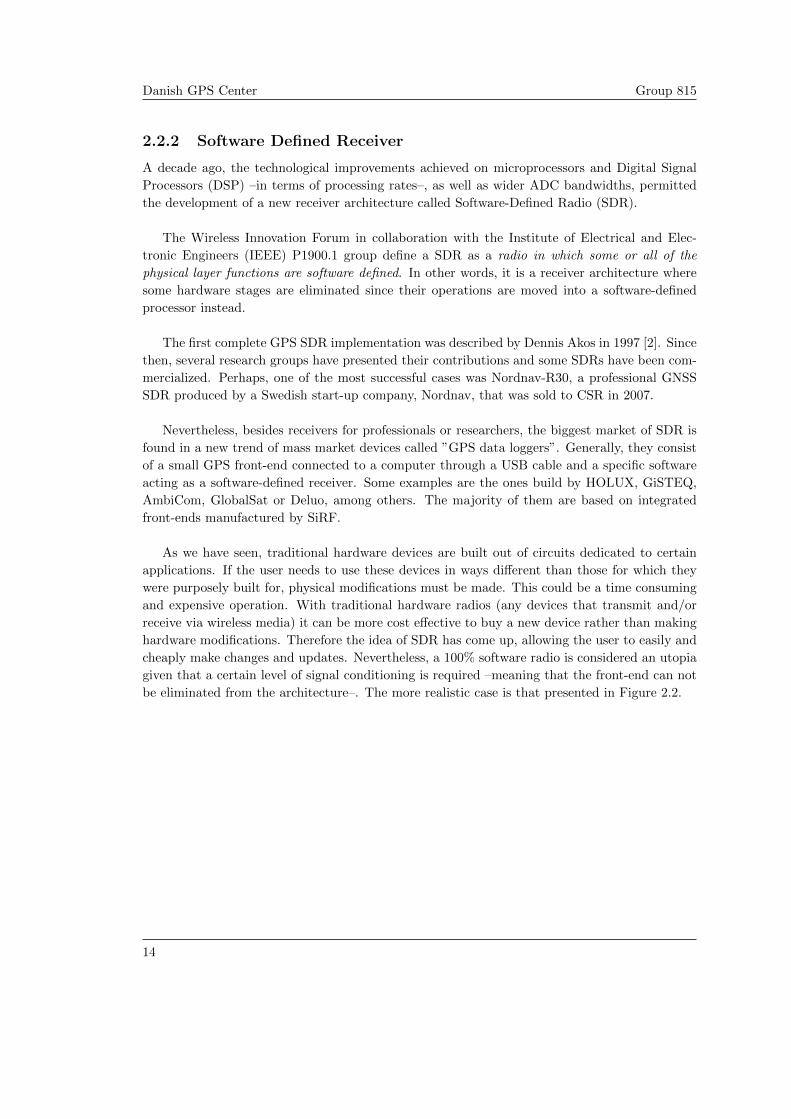
Our development was based on snapshots collected through a GPS RF front-end formed by an

Integrated Circuit (IC) from SiGe semiconductors, the SE4110L, which includes an on-chip Low

Noise Amplifier (LNA) and a low IF receiver with a linear Automatic Gain Control (AGC) and

2-bit analog-to-digital converter (ADC). All these are contained within a 4x4 mm low cost chip

–further description of its specifications can be found in its datasheet [1]–.

Figure 3.1: SiGE front-end photography. It contains SE4110L and a USB interfacing chip.

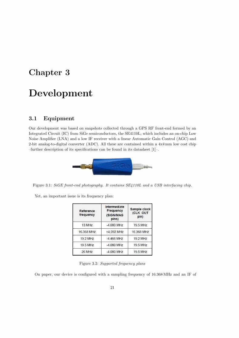
Yet, an important issue is its frequency plan:

Figure 3.2: Supported frequency plans

On paper, our device is configured with a sampling frequency of 16.368 MHz and an IF of

21


4.092 MHz but in practice, our unit has an IF of 4129945 Hz. These are key values limiting the

pseudo-range resolution and, besides that, they must also be taken into account during acquisi-

tion.

Resolution =c

SamplingFrequency≃ 18.32m

The election of the sampling frequency forces to establish a tradeoff between pseudo-range

accuracy and amount of data. Let’s assume for a moment that our snapshots have a length of

20ms, this would mean storing:

Size = SamplingFrequency ⋅ 0.02 = 327.360 kB

Nowadays, most of the hand-held devices use miniSD or microSD memory cards, whose ca-

pacities are often several gigabytes. Therefore, using 1 GB memory card would allow us to store

more than a thousand snapshots. These rough calculations give us a good reason to think about

its potential applications.

3.2 Acquisition Methods

The purpose of acquisition is to determine visible satellites and coarse values of carrier frequency

and code phase. A basic acquisition scheme is presented in Figure 3.3.

Figure 3.3: Basic acquisition scheme, picture taken from [2]

A carrier wave replica must be generated locally in order to recover the original baseband

signal. This is done by multiplying the two waves.

Next, the incoming code should be removed. This can be done only when the code phase of

the signal is known. Due to the high autocorrelation with zero lag proprieties of the PRN code

(see A.2.1), it is possible to remove the incoming code by multiplying it with a locally generated

PRN code replica.

22

Chapter 3. Development 3.2 Acquisition Methods

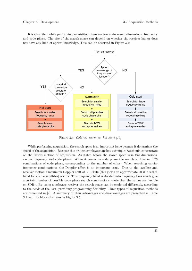
It is clear that while performing acquisition there are two main search dimensions: frequency

and code phase. The size of the search space can depend on whether the receiver has or does

not have any kind of apriori knowledge. This can be observed in Figure 3.4:

Figure 3.4: Cold vs. warm vs. hot start [10]

While performing acquisition, the search space is an important issue because it determines the

speed of the acquisition. Because this project employs snapshot techniques we should concentrate

on the fastest method of acquisition. As stated before the search space is in two dimensions:

carrier frequency and code phase. When it comes to code phase the search is done in 1023

combinations of code phase, corresponding to the number of chips. When searching carrier

frequency combinations, the Doppler effect is an important issue. Due to the satellite and

receiver motion a maximum Doppler shift of ∼ 10 kHz (this yields an approximate 20 kHz search

band for visible satellites) occurs. This frequency band is divided into frequency bins which give

a certain number of possible code phase search combinations –note that the values are flexible

on SDR–. By using a software receiver the search space can be exploited differently, according

to the needs of the user, providing programming flexibility. Three types of acquisition methods

are presented in [2]. A summary of their advantages and disadvantages are presented in Table

3.1 and the block diagrams in Figure 3.5.

23


Figure 3.5: a) Serial search acquisition; b) Parallel Frequency Space search acquisition; c)Parallel

Code Phase search acquisition, see [2]

24


Table 3.1: Acquisition methods, see [2]

Type of acquisition Advantages Disadvantages

Serialsimple 41⋅ 1023 = 41943 search combinations

easy to implement very slow

Parallel Frequency less search combinations more complicated due to FT

space search1023 code phases dependant on FT implementation

faster

Parallel Code Phase least combinations computationally demanding

space search41 frequency bins dependant on FT and IFT implementation

the fastest the most complex

The Serial acquisition is usually used in CDMA systems. The other two methods parallelize

either frequency or code phase parameter in order to minimize the search space. They also

use Fourier transform, adding to their complexity. The most efficient method, namely Parallel

Code Phase search acquisition also uses circular correlation. All three methods use off-line code

generation.

3.2.1 Serial Acquisition

The Serial acquisition is the simplest one to implement. Due to the fact that it does not use

Fourier transform it is also the least computational demanding. As seen in figure 3.5a) the first

step of this type of acquisition is to multiply the incoming signal with a locally generated PRN

code. The in-phase and quadrature signals are obtained by multiplying the resulting signal with

a locally generated carrier signal, and, respectively with a 90∘ shifted locally generated carrier

signal. The last part of the algorithm involves obtaining signal power in both in-phase and

quadrature arms. This algorithm is the slowest one because it sweeps all possible intermediate

frequencies (±10 kHZ corresponding to the Doppler shift) into 500 Hz steps, thus getting 41 fre-

quency bins, plus 1023 different code phases. Due to the fact that 16 samples are used per each

chip of the C/A code we actually get a number of 16368 samples per millisecond.

We proceeded to implement this algorithm and tested it with both simulated GPS signal

and with real snapshots. Figure 3.6 shows the output of the Serial search algorithm with real

snapshot. Due to the fact that this algorithm is very slow, the algorithm has been run only for

five possible PRNs. Space vehicle (SV) 4 is visible and acquired.

25


Figure 3.6: Output of serial search acquisition performed on SV 4

3.2.2 Parallel Frequency Space Search Acquisition

This algorithm provides a faster acquisition method. In this case there exists a tradeoff between

speed and how computational demanding it is, because, as shown in Figure 3.5b), the Parallel

Frequency space search algorithm uses Fourier transform. The basic idea of this type of ac-

quisition is to try to eliminate one of the two search spaces, namely the frequency dimension.

Therefore the search only occurs in the code phase dimension, which means that only the 1023

different code phases are looked into.

The implementation of this algorithm is quite straightforward, following the basic block dia-

gram presented in 3.5b). The incoming signal is multiplied with a locally generated PRN code.

If the two signals perfectly align than the result will be a continuous wave. This takes advantage

of the high autocorrelation and low cross-correlation proprieties of the PRN code (see A.2.1).

Therefore, if the two codes are perfectly aligned, the Fourier transform will result in a distinct

peak.

While implementing this algorithm we observed that the spectrum of the signal power is

symmetric. As stated in [9], when applying Fourier transform to a real input sequence, the first

half of the resulting samples will be redundant with the second half (as shown in Figure 3.7) due

to Nyquist theorem.

26


Figure 3.7: Uncut spectrum

Therefore, in order not to get redundant peaks we cut the spectrum and used only the part

around the intermediate frequency which we needed. The result is presented in Figure 3.8. One

consequence of this is that in the plots presenting the obtained peaks, the frequency index where

the peaks are situated are actually half of the real frequency index.

Figure 3.8: Cut spectrum

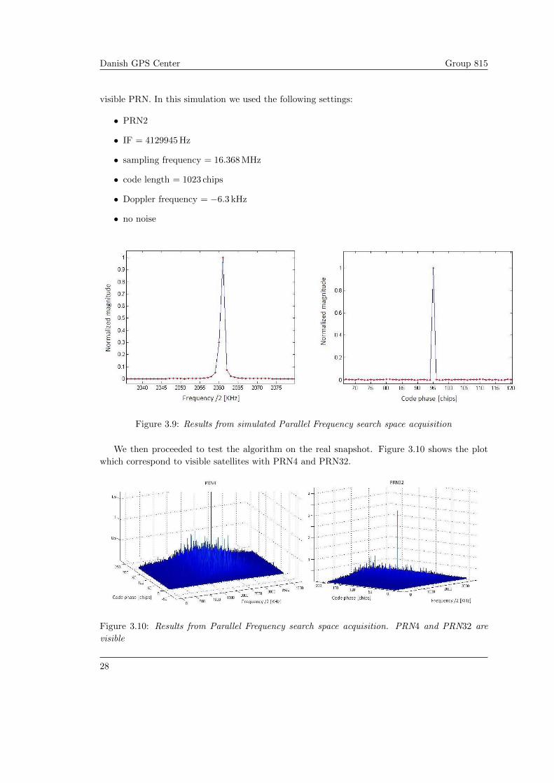
In order to verify the results of the Parallel Frequency space search acquisition algorithm we

first used a simulated GPS signal without adding any noise. The results are presented in Figure

3.9, figure which shows the frequency and code phase of the obtained peak corresponding to the

27


visible PRN. In this simulation we used the following settings:

∙ PRN2

∙ IF = 4129945 Hz

∙ sampling frequency = 16.368 MHz

∙ code length = 1023 chips

∙ Doppler frequency = −6.3 kHz

∙ no noise

Figure 3.9: Results from simulated Parallel Frequency search space acquisition

We then proceeded to test the algorithm on the real snapshot. Figure 3.10 shows the plot

which correspond to visible satellites with PRN4 and PRN32.

Figure 3.10: Results from Parallel Frequency search space acquisition. PRN4 and PRN32 are

visible

28


3.2.3 Parallel Code Phase Space Search Acquisition

This is the fastest method of acquisition out of the three presented in Table 3.1, but the speed

comes with the cost of being very computationally demanding. This method relies on paral-

lelizing the code search space. Therefore we only need to search in the frequency bins. In our

algorithm there are 57 different frequency bins due to our bandwidth and bin width settings. It

is obvious that this is much more effective than searching all 1023 different code phases, or in

both frequency bin and code phase search spaces. As shown in Figure 3.5c) the algorithm uses

both Fourier transform and inverse Fourier transform (IFT). This is what makes the algorithm

computational demanding. The incoming signal is multiplied by a locally generated carrier signal

thus resulting in the in-phase (I) signal. By shifting the carrier signal with 90∘ and multiplying

it with the incoming signal the quadrature (Q) signal is formed. These complex signals are

combined into the sequence x(n) = I(n) + jQ(n) and provided as input for the discrete Fourier

transform function(DFT). The result of this function is multiplied with the complex conjugate

of the locally generated PRN code in frequency domain. The next step is to transform the result

back to time domain via inverse Fourier transform and get the absolute value of the resulting

sequence. It must be taken into account when calculating the power of the signal that the output

of the IFT is complex. Basically, at this stage we realized correlation between the input and the

locally generated PRN code.

The code for this algorithm was taken from [2]. We proceeded in testing the algorithm as in

the case of Parallel Frequency search space algorithm with both simulated GPS signal (with the

same parameters ) and with a real 1 second snapshot.

First we will show the results which were obtained while running acquisition with simulated

GPS signal, both with and without noise in Figure 3.11. This test was made for visible PRN4. It

is clearly visible that even when adding noise we can still obtain a peak which has a magnitude

much higher than the noise, making acquisition possible.

Figure 3.11: Simulated signal Parallel Code Phase space search acquisition results; a)without

noise, b)with simulated noise

29


We proceeded to test the algorithm with a real set of data. Figure 3.12 shows the plots for

visible satellites with PRN4 and PRN32.

Figure 3.12: Results from Parallel Code Phase space search acquisition with real data

All the acquisition techniques presented above were performed on a single C/A period (1 ms).

In order to achieve better acquisition, power integration can be implemented along several C/A

periods.

Basically, there are two different types of power integrations: coherent and non-coherent.

The difference lies on the fact that coherent acquisition integrates the signal separating between

in-phase and quadrature branches, while non-coherent acquisition integrates the signal from its

modulus. As shown in [7] and [8], implementing a coherent type of acquisition should have

advantages over non-coherent acquisition, advantages as higher acquisition success rate, more

useful signal power can be recovered, false alarm reduction, higher detection probability and

lower noise floors.

Even though we invested certain effort investigating this, we will not stress this aspect be-

cause it is beyond the purpose of this project.

3.3 Five State Position Computation Algorithm

This section contains an explanation of the algorithm used to achieve positioning without track-

ing. The algorithm used is described more in detail in [14]. The flow chart of this algorithm is

presented in Figure 3.13.

30

Chapter 3. Development 3.3 Five State Position Computation Algorithm

Figure 3.13: Flow chart of positioning algorithm [14]

[14] examines techniques to achieve sub-second first fix and to overcome situations where

decoding time-of-week (TOW) from the handover word (HOW) is not possible due to signal

weakness. This algorithm is also suitable while using snapshot techniques.

In navigation algorithms there are 4 main steps that need to be done:

∙ start with a-priori estimate of state

∙ predict the pseudo-ranges which would correspond to the above mentioned state

∙ take the actual pseudo-range measurements

∙ update the a-priori state by subtracting the predicted pseudo-range from the actual one

The term “state”is used to define quantities used in the algorithm such as position, time,

velocity and others. The classic navigation algorithms use 4 components to define the state:

three coordinates (x, y, z) and the receiver clock error (b), a common bias for all pseudo-ranges.

Time-keeping issues are crucial in GPS systems. An essential element of this algorithm is

coarse time. By this we understand a time accuracy which is worse than 10 ms. This will yield a

positioning error around or smaller than 8 m, an error which is considered acceptable. Therefore

31


coarse time acts like the time accuracy threshold in order to achieve a position with acceptable

accuracy.

The key of this algorithm is introducing a time bias over the coarse time, as a fifth state

in the navigation equations. Thus allowing convergence towards a precise time starting from a

coarse time. Further on we will present the mathematical description of this situation. We use

superscript in order to relate certain values to different satellites, upper case for vectors, lower

case for scalar values and bold format upper case for matrices. We start by defining the vector

of a-priori state including coarse time as a fifth state:

�X =

⎡⎢⎢⎢⎢⎢⎣�x�y�z�b�tc

⎤⎥⎥⎥⎥⎥⎦ (3.1)

We continue by defining the vector of apriori measurement residuals (�Z) from satellite k

as the difference between the vector of measured pseudo-ranges (Z) and the vector of predicted

pseudo-ranges (Z):

�Zk = Zk − Zk (3.2)

Zk = ∣Xk(ttx)−X0∣ − �tk(ttx) + b0 (3.3)

ttx = estimated time of transmission of measured signal

Xk(ttx) = calculated satellite position at ttxX0 = a-priori receiver position

�tk(ttx) = satellite clock error in unit of length at ttx

b0 = a-priori estimate of common bias

The only term affected by the coarse time in (3.2) is the vector of predicted pseudo-ranges,

and this is described mathematically by (3.4). −vk�tc represents the coarse time error.

Zk(ttx)− Zk(ttx) = Zk(ttx)− Zk(ttx + �tc) = −vk�tc (3.4)

As shown in [14] the relationship between �Zk and X is presented in (3.5). Notice that coarse

time errors, common bias and all measurement errors are taken into account.

�Zk = −ek�Xxyz + �b + vk�tc + "k (3.5)

where:

ek = unit vector from receiver to satellite k

�Xxyz = vector of spatial elements

"k = measurement errors

�tc = update to a-priori coarse time state k

32


vk = pseudo-range rate

So far we are dealing with one satellite. It is a well known fact that in order to have a working

GPS system you have to deal with a minimum of four satellites. Due to the fact that we introduce

the coarse time as a fifth state, in the proposed algorithm for GPS snapshot techniques we have

to deal with a minimum of 5 satellites. Continuing with this hypothesis we have to extend (3.5)

for the number of visible satellites. It is very important to know that the common bias affects

all measurements, all by the same amount, and the coarse time error affects only predicted

measurements, each by different amount [14]. The next step is to introduce these equations in a

matrix equation. This gives the opportunity to solve with the method of least squares. Therefore:

�Z = H�x+ " (3.6)

H =

⎡⎢⎣ −e1 1 v1

......

...

−ek 1 vk

⎤⎥⎦ (3.7)

We can solve for �x through a least squares solution:

�x = (HTH)−1HT �Z (3.8)

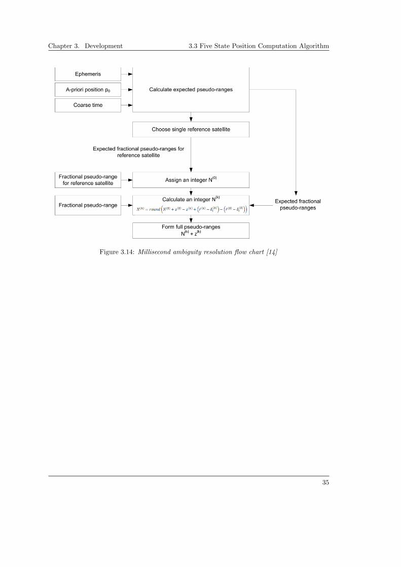
3.3.1 Millisecond Ambiguity Resolution

As stated in section 3.3 we want to achieve positioning before decoding HOW. This implies that

we are only dealing with fractional pseudo-ranges. Therefore arises the need to reconstruct these

pseudo-ranges. This need of reconstruction can also be observed from (3.2) because the vector

of predicted pseudo-ranges Zk has a value which is a multiple of milliseconds while the vector of

measured pseudo-ranges Zk has sub-millisecond values. Due to the fact that the common bias

affects all measurements equally it must be taken into account that this common bias must be

consistent for all measurements while reconstructing the pseudo-ranges.

In order to solve the millisecond ambiguity a reference satellite must be chosen. The reference

satellite will be the one with the largest elevation angle. The next step will be to assign an integer

value (N0) to this satellite. The value chosen for N0 was the value used in [14] which is obtained

by rounding the difference between the multiple millisecond expected pseudo-range and the sub-

millisecond measured ones 3.9. [14] also states that even if this value is not chosen in this way

which makes pseudo-ranges as close as possible, it will not affect the outcome of the algorithm

in a drastic way.

N0 = round(Z0 − Z0) (3.9)

Next the full pseudo-range is reconstructed for the reference satellite:

N0 + Z0 = r0 − �t0 + b+ "0 = r0 + d0 − �t0 + b+ "0 (3.10)

where:

r0 = actual geometric range

33


r0 = geometric range from apriori position

�t0 = satellite clock error

d0 = error in r0

b = common bias

"0 = measurement errors

We rewrite (3.10) for the rest of the measurements:

Nk + Zk = rk − �tk + b+ "k = rk + dk − �tk + b+ "k (3.11)

After subtracting (3.10) from (3.11) we get:

(Nk + Zk)− (N0 + Z0) = (rk + dk − �tk + b+ "k)− (r0 + d0 − �t0 + b+ "0) (3.12)

Nk = N0 + Z0 − Zk + (rk + dk − �tk + b+ "k)− (r0 + d0 − �t0 + b+ "0) (3.13)

Because the common bias affects all measurements in exactly the same way it is plain to see

that it cancels. Therefore we get:

Nk = N0 + Z0 − Zk + (rk − �tk)− (r0 − �t0) + (dk + "k − d0 − "0) (3.14)

The only term which is not known in (3.14) is (dk + "k− d0− "0) which represents the effects

of measurement errors and of the errors in the predicted measurements. [14] describes in detail

why this term can be excluded from our computations. Its value is less than half of millisecond so

it can not be taken into account. This is how we get to the final form of this equation, equation

which now can be solved because all variables are known or can be computed:

Nk = round[N0 + Z0 − Zk + (rk − �tk)− (r0 − �t0)] (3.15)

Finally we just have to form the full pseudo-ranges Nk + Zk. Figure 3.14 shows the flow

chart of the millisecond ambiguity resolution algorithm.

34


Figure 3.14: Millisecond ambiguity resolution flow chart [14]

35

Chapter 4

Experimental Results

This chapter describes the most interesting experiments realized during development. Basically,

there are two main lines of experiments:

∙ acquisition methods performance

∙ sub-second positioning results

4.1 Acquisition Methods

Initially we focused our efforts on testing and studying acquisition algorithms, owing to the fact

that they are a limiting factor on the performance of snapshot techniques, affecting both the

pseudo-range accuracy and the satellite acquisition.

4.1.1 Execution Time Comparison

This section contains a comparison of the execution time for each of the three acquisition al-

gorithms presented in 3.2. All timing results where obtained using the Profiler tool integrated

in Matlab and are based on a snapshot (taken on 02/03/2010 at 12:14:02 UTC) of 1 ms length,

collected with the front-end presented in 3.1. The search space was equally set for all algorithms,

forming a 2D grid sweeping ±14 kHz around the IF carrier with 500 Hz step and 1023 chip shifts

of the C/A code. Obviously, if the search space and/or the resolution increases –this means

reducing the frequency step, providing more frequency bins–, the execution time increases pro-

portionally for all methods.

The results are presented in Table 4.1 in terms of elapsed time and number of loops to be

executed by the routine.

36

Chapter 4. Experimental Results 4.1 Acquisition Methods

Table 4.1: Acquisition methods performance comparison

Acquisition method Execution time [s] Search space [loops]

Parallel Code Phase space search 27.465 57

Parallel Frequency space search 124.725 1023

Serial 1504.576 58311

Interpreting these results, one verifies the theoretical concepts described in 3.2.

Serial acquisition was ruled out for further testing in next subsections due to its massive exe-

cution time. In fact this was an optimized version of the algorithm. The execution time obtained

for the first implemented version of the Serial acquisition algorithm was even larger (3466.089 s).

Even though providing correct solutions, it was clear that the code could be optimized. After

debugging with Profiler, we noticed that there was high redundancy while generating copies of

the local carrier waves, which significantly increased the code execution time.

In addition, we investigated the main factors conditioning the execution time for each algo-

rithm. The results of this are presented in Table 4.2.

Table 4.2: Functions which influence execution time, and their contribution

Acquisition method Function Contribution[%]

Parallel Code Phase Fourier and Inverse Fourier Transforms 80.3

Parallel Frequency Fourier Transforms 53.4

Serial Local carrier wave generation 40

It turns out that the Fourier Transform (FT) and the Inverse Fourier Transform (IFT) opera-

tions, although resulting in faster algorithms, demand the greatest computational effort. On the

other hand, in the Serial acquisition, most of the computational load was invested in generating

the local carrier waves used to demodulate the signal from the carrier wave.

4.1.2 Acquisition Statistics

The following set of experiments is meant to illustrate the actual ability of the algorithms when it

comes to detecting SVs. Basically there are three possible solutions resulting from the acquisition

evaluation. A SV can be:

∙ detected – visible and acquired

∙ undetected – visible but not-acquired

∙ false alarm – not visible but acquired

Although theoretically there is a certain fixed amount of dBc between the main correlation

peak and the nearest peaks, in real applications this value is unknown given the noise level and

37


signal fading. Thus, in practice, all implemented algorithms decide upon acquisition using a

threshold describing the ratio between the main and the secondary lobes –which is a way to

measure carrier to noise ratio (C/N0)–. If the actual ratio is bigger than the threshold, the

algorithm interprets that a GPS signal is present.

Therefore, the selection of an appropriate threshold is a critical choice affecting the perfor-

mance of the algorithm. In order to evaluate its impact and determine an optimal value, we

have generated statistics about the three possible evaluation solutions presented above. The

simulation was based on the same snapshot used in the previous subsection, and the acquisition

results were collected along 100 consecutive milliseconds of the snapshot (the integration time

being kept at 1 ms which produces 100 cases).

Thanks to the broadcasted 24h Receiver INdependent EXchange (RINEX) navigation files,

one is able to recompute the position of any SV at a given time instant. This allows us to

simulate the sky scenario by the time the snapshot was taken. The following figure shows a plot

of the satellites in view on the 2nd of March of 2010 at 12:14:05 UTC in Aalborg University.

Figure 4.1: Sky plot on 02/03/2010 at 12:14:05 UTC generated in Matlab from a RINEX file.

A green star represents a healthy SV while a red star indicates unhealthy SV, the yellow line

represents the elevation mask.

In order the check our SV positioning results, we used a trusted and widespread program

among satellite observers, Orbitron.

38


Figure 4.2: Sky plot on 02/03/2010 at 12:14:05 UTC simulated with Orbitron

Apart from a visual check, the numerical comparisons also showed the validity of our code.

So, selecting an elevation angle of 0∘, our scenario is composed by 11 SVs –PRN 1, 4, 11, 12, 13,

17, 20, 23, 30, 31 and 32– out of 32. The figure below shows the Parallel Code Phase acquisition

results as a function of threshold.

Figure 4.3: Parallel Code Phase acquisition results as function of the threshold value. Green

represents acquired SV, blue indicates non-acquired SV and red means false alarms. The dashed

line is the total number of visible SVs

39


It is quite interesting to observe the exponential behavior of the false alarms as soon as the

threshold gets below the value of 2.5. Above it, the acquired signals decrease in favor of the

non-acquired ones, so there is a clear compromise between the accepted false alarm level and the

acquired and non-acquired SVs that sets an optimal threshold around 2.5.

Concerning the Parallel Frequency acquisition, the results showed in Figure 4.4 indicate that,

regardless any threshold, its overall performance is inferior due to a higher level of false alarms

and an earlier crossing point between acquired and non-acquired SVs.

Figure 4.4: Parallel Frequency acquisition results as function of the threshold value. Green

represents acquired SV, blue indicates non-acquired SV and red means false alarms. The dashed

line is the total number of visible SVs

The explanation of these results may rely on the GPS signal structure itself, since the code

correlation presents better results than a frequency search in terms of absence of secondary

lobes. As described in subsection A.2, the C/A code is a square wave that has triangular shape

autocorrelation results. However, due to Fourier Transform properties, any time-frequency trans-

formation computed from a carrier wave represented with a finite number of samples will result

in a Sinc function –meaning the presence of signal lobes–. This fact implies that a lower threshold

value shall be used in acquisition.

In order to illustrate this fact, we have simulated an ideal case of signal search without noise.

40


Figure 4.5: Frequency-Code phase search area. The code phase axis has been cut to around

163 samples out of 16368. The frequency axis is formed by 160 bins resulting from a ±4 kHz

bandwidth divided by 50 Hz steps.

Figure 4.6: Both figures represent a cut containing the maximum peak but along different axis.

Left: Frequency axis. Right: Code phase axis

On the other hand, in a real situation there are some other inconveniences like the presence of

white noise –quite visible in Figure 3.8– and the accidental generation of signal spurious during

frequency down-conversion by the front-end. All these factors are contributing to a higher false

alarm level.

41


Another interesting fact was to observe that the non-acquired SVs were exactly the ones with

lower elevations, which fits with the fact that they are farther, and so, the signals are weaker,

resulting in low carrier to noise ratio (C/N0).

From here after, we decided to keep using only Parallel Code Phase acquisition since it is the

fastest and the most reliable algorithm from the ones we have implemented and tested.

4.1.3 Enhancing Acquisition Performance

Basically, the acquisition performance is broken down into two different aspects:

∙ The ability of the algorithm to acquire line-of-sight satellites: The ideal scenario would

be to detect all visible satellites without triggering any false alarms. This is the most

important factor since the positioning accuracy is tightly related with the number of SVs

(each one providing a pseudo-range measurement into the observations equation) and their

geometrical dilution of precision (GDOP), which directly depends on this specific capability

of the algorithm.

∙ Accuracy of code-phase and Doppler frequency values: Typically, acquisition is meant to

compute rough values that would be used as “starters”for tracking stages, in order to

refine them. However, in snapshot techniques tracking is omitted, thus the pseudo-range

accuracy relies on acquisition. Nevertheless, given that our particular front-end offers a

pseudo-range resolution ≈ 18 m (as stated in section 3.1), we believe it will be good enough

for our application.

Hence, we will focus on methods to improve acquisition performance in terms of the first

aspect detailed above.

As we have described in 4.1.2, the threshold value is a way to measure C/N0. So assuming that

our threshold value is an optimal one –in the sense of detection to false alarm rate–, the only way

to improve our acquisition algorithm is to, somehow, increase C/N0 after correlation. A common

technique for that purpose consists in power integration along several periods of the signal. This

is possible assuming that code-phase and Doppler frequency values will not vary considerably

from one period to the consecutive ones. Thanks to the short period of the C/A signal –1 ms–

this conditions are ensured. On the one hand, the clock stability of a GPS receiver is required to

be better than 10ppm [11] –this guarantees code-phase stability and reliable Doppler frequency

measurements–, on the other hand, the Doppler drift rate, due to constellation dynamics, is way

too small to create considerable differences from one period to the consecutive ones. Only high

dynamics of the receiver could cause certain trouble but a snapshot taken from a photo camera

cannot be considered to suffer from this issue. Therefore, we believe power integration to be a

solid candidate to improve acquisition performance.

This subsection presents experimental results of non-coherent power integration implemented

over Code-Phase Parallel acquisition. Their main benefits and drawbacks will be discussed and,

finally, new settings of their parameters will be investigated for the purpose of our application on

42


photo cameras. The non-coherent power integration was chosen for being the simplest form of

power integration, given that is computed as the integral of the in-phase and quadrature power

modulus, while a coherent acquisition shall be computed as a different power integral for each

branch and further time-frequency transformations are to be considered.

All experimental results were computed using the same snapshot utilized in the previous

subsection 4.1.2. Due to the fact that we are dealing with discrete values, the power integration

is in fact a summation of the signal powers obtained over several milliseconds.

Figure 4.7 clearly shows that the new acquisition algorithm improves C/N0, which pretends

to minimize the noise floor. In particular, its results were computed with an integration time

of 20 ms –20 periods of the C/A code–. The plots show normalized values to avoid confusion

induced by different absolute magnitudes resulting after each method.

Figure 4.7: PRN4 code-phase axis after correlation ; a) Parallel Code Phase, b)Power Integration

Parallel Code Phase

In order to provide some numerical relation between integration time and C/N0 improvement,

Figure 4.8 shows the values of the peak metric (corresponding to PRN 32) obtained along different

integration time intervals. On top of the experimental results, a logarithmic trend line showed to

be the best fitting function. It is obvious that with the growth of the integration time, the peak

metric value is increasing, tending a certain asymptotic value depending on the received power.

43


Figure 4.8: Peak metric vs. integration time

Consequently, by improving the acquisition sensitivity we were able to acquire three more

satellites (PRN 12, 13 and 30) than with the previous acquisition algorithm. During our experi-

ments we observed that the apparition of these satellites is strongly dependant on the integration

time. Table 4.3 shows the minimum integration time that was necessary in order to acquire cer-

tain satellites. Theoretically, as the elevation angle of the satellites decreases, the integration

time should increase to compensate for its signal fading, fact which appears to be confirmed.

Table 4.3: Visible satellites data

PRN Altitude [km] Azimuth [∘] Elevation [∘] Minimum integration time [ms]

20 20084.680 151.8 85.2 1

32 20529.970 86.8 52.9 1

23 20320.940 192.9 47.0 1

17 20158.440 262.1 37.0 1

11 20326.390 163.9 31.2 1

31 20303.740 65.9 30.6 1

04 19995.160 301.8 26.1 1

13 20186.620 205.2 18.8 3

12 20255.390 347.5 9.2 4

30 19883.160 17.3 6.7 7

01 20081.220 38.9 2.1 −

44


From these results we draw the conclusion that an integration time of 7 ms is enough in order

to acquire 10 out of the 11 visible satellites shown in 4.2. And Figure 4.9 shows that 7 ms allows

us to detect SVs with an elevation as low as ≈ 7 ∘ over the local horizon, in this particular case,

PRN30. Obviously, higher integration times will provide slightly better results but this will come

to the price of higher execution times.

Figure 4.9: PRN30 peak metric versus integration time

So after analyzing these results one concludes that 7 ms offers the best trade off between

number of detected satellites and computation time. Due to its better performance we have used

this method in our future experiments, and so we update Table 4.1 getting Table 4.4. The size of

the search space in the case of the power integration algorithm comes from the multiplication of

the original search space–the actual number of frequency bins– with the number of milliseconds

to process.

Table 4.4: Acquisition methods performance comparison–updated version

Acquisition method Execution time [s] Search space [loops]

Parallel Code Phase 27.465 57

Power Integration Parallel Code Phase 136.355 399

Parallel Frequency 124.725 1023

Serial 1504.576 58311

After these results, we decided to repeat the statistical analysis presented in 4.1.2 in order

to observe the number of acquired, non-acquired satellites and false alarms achieved by this

algorithm as a function of the threshold value. Due to the longer execution time we collected

results from 80 consecutive 7 ms samples of the snapshot, instead of 100 samples collected in

subsection 4.1.2. The obtained results are shown in Figure 4.10. It is interesting to notice the

maximization of the “acquisition window”thanks to C/N0 improvement after power integration

–compare with Figure 4.3–, and that the false alarm exponential falls earlier, leading to a lower

optimum threshold value than in the case of the Parallel Code-Phase or the Parallel Frequency.

45


As it can be observed, in this case a more appropriate value for the threshold is 2. Statistically,

this value provides ≈ 0 false alarms, and 10 acquired satellites versus 1 non-acquired satellite

out of 11 –this satellite (PRN1) has a very low elevation angle as seen in 4.3–.

Figure 4.10: Power Integration Parallel Code Phase acquisition results as function of the thresh-

old value. Green represents acquired SV, blue indicates non-acquired SV and red means false

alarms. The black line is the total number of visible SVs.

This proves that the power integration algorithm gives better performance than single period

acquisition algorithms. So, despite its higher execution time, we decided to use the “Non-

Coherent Power Integration Code-Phase Parallel acquisition”along all the positioning experi-

ments presented below due to its reliability.

4.2 Positioning Results

Once an acquisition algorithm stable enough has been achieved, in the sense of results repeatabil-

ity from one period of the snapshot to the following ones, it was time to prove the performance of

the real core algorithm of the project, the coarse-time navigation presented in section 3.3. This

was the trickiest part of the project causing most of the implementation problems.

The experimental results were obtained from a small testbed formed by 6 different snapshots

which are presented in Table 4.5:

46

Chapter 4. Experimental Results 4.2 Positioning Results

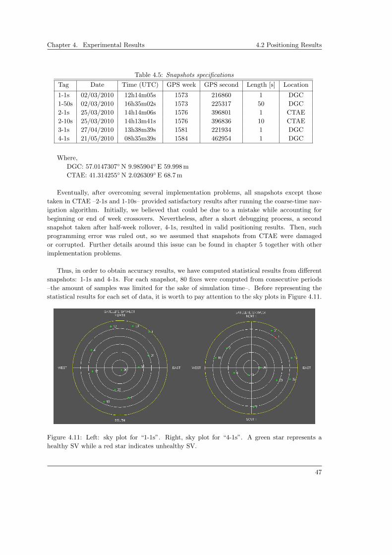
Table 4.5: Snapshots specifications

Tag Date Time (UTC) GPS week GPS second Length [s] Location

1-1s 02/03/2010 12h14m05s 1573 216860 1 DGC

1-50s 02/03/2010 16h35m02s 1573 225317 50 DGC

2-1s 25/03/2010 14h14m06s 1576 396801 1 CTAE

2-10s 25/03/2010 14h13m41s 1576 396836 10 CTAE

3-1s 27/04/2010 13h38m39s 1581 221934 1 DGC

4-1s 21/05/2010 08h35m39s 1584 462954 1 DGC

Where,

DGC: 57.0147307∘ N 9.985904∘ E 59.998 m

CTAE: 41.314255∘ N 2.026309∘ E 68.7 m

Eventually, after overcoming several implementation problems, all snapshots except those

taken in CTAE –2-1s and 1-10s– provided satisfactory results after running the coarse-time nav-

igation algorithm. Initially, we believed that could be due to a mistake while accounting for

beginning or end of week crossovers. Nevertheless, after a short debugging process, a second

snapshot taken after half-week rollover, 4-1s, resulted in valid positioning results. Then, such

programming error was ruled out, so we assumed that snapshots from CTAE were damaged

or corrupted. Further details around this issue can be found in chapter 5 together with other

implementation problems.

Thus, in order to obtain accuracy results, we have computed statistical results from different

snapshots: 1-1s and 4-1s. For each snapshot, 80 fixes were computed from consecutive periods

–the amount of samples was limited for the sake of simulation time–. Before representing the

statistical results for each set of data, it is worth to pay attention to the sky plots in Figure 4.11.

Figure 4.11: Left: sky plot for “1-1s”. Right, sky plot for “4-1s”. A green star represents a

healthy SV while a red star indicates unhealthy SV.

47


The scenario on snapshot “1-1s”is formed by 11 SVs in a rather good distribution on the sky.

Furthermore, we know from previous tests, that in such scenario, our acquisition routine is able

to acquire 10 our of 11 of these satellites, which leads us to expect relatively good positioning

accuracy caused by a favorable GDOP. On the other hand, the scenario on snapshot “4-1s”is

also formed by 11 SVs but one of them was set as unhealthy, so it was not used during coarse-

navigation. Apart from that, the distribution of the satellites is not as uniform as in “1-1s”and

we observed that acquisition function was detecting an average of 8 SVs, PRN1 among them,

which leaves this scenario with a worst GDOP and 7 useful measurements. For these reasons,

one would expect to find better accuracy using snapshot “1-1s”than “4-1s”.

The figures below show the accuracy results computed from both snapshots.

Figure 4.12: Positioning results plotted on Google Earth. Green dot: Actual position of the

antenna. Red dots: fixes from snapshot “4-1s”. Blue dots: fixes from snapshot “1-1s”. All

samples are grabbed to the ground level.

48


Figure 4.13: Horizontal Positioning Error. Red dots: fixes from snapshot “4-1s”. Blue dots:

fixes from snapshot “1-1s”.

Figure 4.14: Vertical Positioning Error. Red dots: fixes from snapshot “4-1s”. Blue dots: fixes

from snapshot “1-1s”.

49


Figure 4.15: Histogram of Horizontal Positioning Error. Each bar represents the number of cases

within the same error margin. Red: “4-1s”. Blue: “1-1s”.

Figure 4.16: Histogram of Vertical Positioning Error. Each bar represents the number of cases

within the same error margin. Red: “4-1s”. Blue: “1-1s”.

As predicted, the horizontal accuracy is much better for snapshot “1-1s”than “4-1s”results.

However, the vertical accuracy of “1-1s”, although less dispersive, is worse than “4-1s”given to

a height bias clearly visible in Figure 4.14 and Figure 4.16. Table 4.6 serves as a numerically

summary of the accuracy results.

50


Table 4.6: Positioning statistics from snapshot “1-1s”. HPE stands for Horizontal Positioning

Error. VTE means Vertical Positioning Error

ID � HPE � HPE 2� (95 %) HPE � VPE � VPE 2� (95 %) VPE

1-1s 8.28 3.72 14.64 39.85 14.66 64.88

4-1s 29.47 11.38 47.48 11.81 15.93 38.14

Besides these minor differences among snapshots, the overall accuracy fit with the require-

ments of our application and results from other studies [5] and theory [14].

4.2.1 Convergence Strength Solving for Millisecond Integer Ambiguity

In the previous paragraphs, some accuracy results have been presented after assisting the coarse-

navigation algorithm with the proper ephemeris (from daily 30-second RINEX navigation file),

and the actual time and coordinates of the taken snapshot. Nonetheless, the greatest feature

of the coarse-navigation algorithm is its convergence strength facing biased assisted time and

coordinates. In other words, it is able to provide a fix with similar accuracy even if the assisted

parameters are corrupted by a certain amount of error.

Theoretically, the boundaries of the assisted data that will cause incorrect millisecond inte-

gers are around 100 km of bias on apriori coordinates guess and 1 minute of bias on the snapshot

time [14]. The present subsection analyzes the flexibility allowed on these assisted parameters

through experiments computed with real data.

Resistance Towards Wrong Apriori Coordinates

To test this aspect, the coarse-time navigation algorithm was feeded with what is believed to be

the actual time when the snapshot was taken, plus an apriori component biased by an increasing

distance. Owing to the fact that distance is just the modulus of a vector, we decided to run two

simulations:

∙ the first one inducing a distance bias along North-South axis

∙ the second one through East-West axis, which would also provide us the means to evaluate

whether the direction has any influence or not.

51


Figure 4.17: Distance between fix and real coordinates versus distance bias on apriori coordinates.

0 s in the horizontal axis represents the actual coordinates where the snapshot was taken.

Figure 4.17 shows the fixes computed by the coarse-time algorithm after introducing a biased

distance. It turns out that, for this specific snapshot, the algorithm is able to converge close to

the actual position coordinates within a bias range compressed from 86 km west until 55 km east,

and between 93 km south and 80 km north. Note that outside this ”convergence window“, the

distance values diverge in discrete steps due to wrong integer millisecond ambiguity resolution.

Figure 4.18: Google Earth plot of apriori coordinates used to test the algorithm. The green

sample represents the actual position of the antenna. Yellow: samples with induced distance

bias towards North. Red: samples with induced distance bias towards East. Distance biases

take values within ±150 km. Black and white area represents the apriori coordinates that would

cause algorithm divergence.

Figure 4.18 gives a better understanding of the area within an apriori position which will drive

the algorithm to a valid fix –we strongly believe anybody would be able to provide approximate

52


coordinates of a photo within this distance range!–.

Figure 4.19: Zoom In to samples within the “convergence window”in Figure 4.17.

Figure 4.19 zooms into Figure 4.17, and one is able to evaluate the accuracy of the positioning

fixes, which in any case are better than 300 m. Note that positions from a bias through north-

south axis present an inflexion point close to the actual position. Unfortunately, this cannot be

appreciated in Figure 4.20 since all samples are grabbed to the ground and such distance bias

had a main contribution in height.

Figure 4.20: Google Earth plot of samples in Figure 4.19. The green sample represents the actual

position of the antenna. Yellow: fixes from samples with induced distance bias towards North.

Red: fixes from samples with induced distance bias towards East. All samples are grabbed to

the ground.

53


It is worth to say that other experiments for different snapshots showed similar behaviors and

accuracies. So, we conclude that the algorithm responds to bias on apriori coordinates according

to theoretical hypothesis.

Resistance Towards Bias on Assisted Time

The tests which will follow are based on the same concept used in the previous results but, in

this case, the coarse-time algorithm was supplied with the actual coordinates of the antenna plus

a time component increasing its bias.

Figure 4.21: Distance between fix and real coordinates versus bias on assisted time. 0 s in the

horizontal axis represents the actual time when the snapshot was taken.

Analogous to Figure 4.17, Figure 4.21 shows the “convergence window”resulting from a time

bias. For this particular snapshot, the algorithm was able to cope with an approximate time

bias of ±100 s, which is quite a long time, more than 3 minutes. The Figure below plots all fixes

achieved from biased time guesses. In any case, its error exceeds 700 m, but other snapshots

returned slightly bigger errors, which demonstrates that providing a “precise”assisted time is

much more demanding than an accurate apriori position fix.

54


Figure 4.22: Zoom In to samples within the “convergence window”in Figure 4.21.

Perhaps this would be one of the most problematic issues in the real application, since it

means that the clock of the camera shall be coordinated with GPS time within this time span.

Assuming than the clock of the camera is stable enough to acquire GPS signals, which required

better than 10 ppm [11] time-keeping accuracy, in the worst case, after synchronization, the

clock would exceed the time boundaries –±90 seconds– after ≈ 100 days. Nevertheless, the in-

ternal clock could be re-synchronized each time the camera is connected to a laptop, computer

or, alternatively, coordinated with the GPS signal itself by decoding the TOW from time to time.

55

Chapter 5

Implementation Discussion

This chapter will present some of the issues and problems we encountered while working on this

project. Some of these were successfully solved while some of them require further work and

investigation.

Firstly we would like to talk about our time organization. Although we know that acquisition

is an important issue in our project, we feel that we invested too much time on it. Therefore

we believe that we should have been a little bit more organized or guided from this point of

view, and we should have spent more time on the core of the problem which is the coarse-time

navigation positioning algorithm [14].

While implementing the coarse-time algorithm certain problems came up. Further on we

would like to describe some of these issues and the way in which they were solved.

One of the first problems we encountered was due to the fact that we made a programming

error while computing satellite speed. In order to identify the problem we made a comparison

with the trusted Orbitron software, which, among other data, also provides information about

pseudo-range rate –what we actually aim to compute–. While programming this algorithm, GPS

toolkit was used as a main reference, which is an open C library. A detailed description of

this library can be found in [13]. After debugging the obtained results with the ones provided

by Orbitron and after consulting the GPS toolkit we realized that our problem consisted in a

trigonometric error on a rotation matrix.

After solving the satellite speed computation error we found that our algorithm was still

not providing satisfactory results. Eventually we realized that while computing the estimated

pseudo-ranges we committed a mistake applying the satellite clock corrections. The bug was

not made in the clock correction algorithm itself, but it was an indexing error affecting the cor-

rections which were applied to each satellite measurements. Summarizing, we were computing

proper clock corrections for all satellites, but we were applying only one of them to all satellites.

These were some of the problems we had which were worth mentioning. Fortunately we

succeeded to resolve them, resulting in a working algorithm. On the other hand we still have an

56

Chapter 5. Implementation Discussion

unresolved issue. For testing purposes we took a snapshot in Viladecans, Spain (41.314255 ∘N

2.026309 ∘E). While the algorithm was working with snapshots taken in Aalborg from the DGC

(57.014733 ∘N 9.9859139 ∘E) we obtained bad results with the one taken in Spain. At first we

thought that we are dealing with an error related to time, due to the beginning or end of week

crossover, because the snapshot was taken on a Thursday –after half week–. After applying the

necessary corrections, the algorithm was still not providing satisfactory results. To verify that

the corrections we made were correct we also took a snapshot on a Friday from the DGC. The

obtained results were satisfactory which lead us to think that the problem must have occurred

while getting the snapshot, most probably due to a hardware failure. Unfortunately we could

not take the snapshot from Spain again, therefore we can not have a precise answer about this

issue.

57

Chapter 6

Conclusions

The present project aimed to study and implement algorithms for GPS snapshot techniques. To

serve that purpose more specifically, we focused ourselves on a single application, digital photog-

raphy geo-tagging.

Summarizing, our problem scope 2.4.3 stated three specific aspects to be implemented or

studied along this project: positioning accuracy versus snapshot length, acquisition performance

versus processing load and degree of assistance. Judging by the achieved experimental results,

we believe that at least the two last aspects have been covered. On the other hand, positioning

accuracy versus snapshot length was covered, somehow indirectly, by the statistical acquisition

results. In other words, this was not achieved by refining code-phase and frequency values, but

by improving its satellite detection capability through power integration.

Concerning acquisition results, we may conclude that the power integration –at least the

non-coherent one– is the most effective technique in terms of statistical stability. Experiments

showed that the threshold value shall be 2 and the integration period shall be 7 ms –which fits

with real implementations like FastLocTM ; 8 ms in that case–, in order to get optimal results.

Furthermore, despite being slower than single period integration, it is much faster than Fre-

quency Parallel and Serial acquisition.

Positioning results, on the other side, have shown that the coarse-time navigation algorithm

provides accuracies within the expected range –20 − 50 m– and it is strong enough to converge

under biased assisted data –about 100 km error in apriori guess and ±90 s bias in snapshot record

time–. However, time bias has a bigger repercussion than apriori guess in the algorithm’s out-

come. So it was shown that GPS snapshot techniques can be used in order to obtain positioning

with acceptable accuracy in order to be used as photo-taggers on digital cameras.

From an academical point of view, working on this project lead us to study GPS related

processing concepts that were not covered in depth in the last semester, therefore aspects which

were new to us.

The reader should take into account that this is a student project, therefore not all techno-

58

Chapter 6. Conclusions

logical aspects have been studied or applied. Further work and analysis should be done in order

to get closer to the actual possibility of creating a new product, some of these being presented

in 7.

59

Chapter 7

Future work

In this chapter we would like to present what future work should be done in order to get closer

to the possibility of creating a new product, a product which would make geo-tagging on digital

cameras possible in a cheap way, with a minimum of required hardware .

One of the things we still consider that it has to be done is a visual interface. Because the

final product is addressed to a wide public this interface should be intuitive and easy to use,

allowing even a non-trained user to be able to work with it. It would be interesting if the user

is given the possibility by this interface to plot results directly on specialized software such as

Google Earth.

As stated before, the final product is not addressed only to GPS experts and engineers.

Therefore the users’ work should be minimized. This is why some software should be devel-

oped that is able to detect the snapshot meta-data and automatically download all the necessary

assisted data. This can be done in a transparent or visible way, according to the needs of the user.

Right now the smallest snapshot we are dealing with is 1 s long which needs 16 MB storage

capacity. This brings up the need of large storage spaces if we think of the number of photograph

which can be taken with a digital camera today. The length of the actual snapshots is controlled

by the driver of the front-end. As shown we just need 11 ms of data in order to achieve positioning

within our expected accuracy range (20−50 m). Therefore the driver should be modified in order

to be able to get just 11 ms long snapshots. This would greatly minimize the needed storage space.

These are just some of the possible improvements which we consider that are to be made in

order to obtain a product which makes geo-tagging on digital photographs possible.

60

Appendix A

Brief Signal Description

GPS provides two levels of service a Standard Positioning Service (SPS) for general public use

and a Precise Positioning Service (PPS) primarily intended for use by the Department of Defense.

This leads to the use of channel access methods for blocking unauthorized users. Specifically,

GPS signals are modulated using Code Division Multiple Access (CDMA) techniques. Thus, the

original spectrum contained 3 different signals allocated over two carriers:

∙ L1 at 1575.42 MHz

∙ L2 at 1227.60 MHz

The PPS service is formed by two encoded signals: P1 and P2 located over L1 and, respec-

tively, L2 –’P’ stands for Precise code–. Dual-frequency signals allow PPS users to correct for

the ionospheric delay, one of the main error sources of the system. Only authorized users know

the code words, allowing them to recover signals from encryption. On the other hand, civil SPS

consists on a unique signal modulated with public Coarse/Acquisition (C/A) codes over L1.

Figure A.1: CA spectra as seen from the receiver’s antenna.

61


Even though DoD foresees the introduction of new civil and military signals in the forthcom-

ing years –usually referred as GPS modernization–, our project focuses exclusively towards the

use of the C/A code signal over L1, owing to the fact that this is the only operative civil signal

and dual-frequency front-ends are currently not feasible for mass market applications.

Therefore, next subsections will provide further details of C/A signal structure along their

generation steps. Understanding its generation turns out to be a key point to understand its

demodulation in the receiver.

A.1 C/A Code Generation

CDMA techniques imply a set of pseudo-noise words or code words. Each word is formed by a

certain number or chips –a chip represents a bit in the context of a pseudo-noise word–. These

words serve the purposes of any spread-spectrum technique: spread the signal along the fre-

quency domain increasing its bandwidth, thus increasing resistance to natural interference and

jamming, and to limit power flux density (note that in figure A.1 the received signal power is

below the noise floor).

Gold codes are used due to their low cross-correlation among the 32 different sequences as-

signed to GPS satellites and their relatively simple implementation. The C/A code has a chip rate

of 1.023 Mcps and a code period of 1023 chips. The somewhat unusual code rates of 1.023 Mcps

are selected so that the period of the C/A code corresponds exactly to 1 ms for time-keeping

purposes [12].

The block diagrams below show C/A code generation step-by-step:

Figure A.2: GPS code generators for satellite i [12]

62

Appendix A. Brief Signal Description A.1 C/A Code Generation

Figure A.3: G1 shift register generator configuration [11]

Figure A.4: G1 shift register generator configuration [11]

Besides the C/A code, the real content of the signal is the navigation message. So it is impor-

tant to note that this is the only source of information, whereas the C/A code is just a manner

to spread the signal and provide the time-transfer feature between the satellites and the receivers.

This report does not include an explanation of the navigation message content because snap-

shot techniques do not require their demodulation. However a detailed description of its contents

can be found in [11].

63


A.2 C/A Signal Modulation

Any signal to be transmitted or radiated through air and space must be modulated into Radio

Frequency (RF). This creates the need of modulating a digital signal over a carrier wave. For

that purpose, GPS uses Binary Phase Shift Key (BPSK), which is a kind of angular modulation

that consists on phase variation of the carrier wave by two discrete values.

Figure A.5: C/A signal modulation

Figure A.6: C/A spreading

The figures above summarize the modulation process. The first one is a representation of the

mathematical/logical operations and the second one shows a graphic explanation of the signal

shape and transformation on each step, especially useful to comprehend the BPSK modulation.

A.2.1 C/A Code Correlation Proprieties

The most important characteristics of the C/A codes are their correlation proprieties [2]. By

correlation we can understand a parameter which describes the degree of independency between

signals in the receiver. If the value of this parameter is high (in our case maximum 1023) that

64

Appendix A. Brief Signal Description A.2 C/A Signal Modulation

means that the signals have a high degree of dependency to one another. If the value reaches

the maximum value it means that the signals are identical. It is obvious to state that if the

value of the parameter is low, the degree of independency is high. In GPS, when dealing with

correlation, high values represent a good alignment of an incoming signal with a locally generated

code. As presented in [2], when talking about correlation we are dealing in fact with two types

of coefficients:

∙ Cross-correlation

∙ Autocorrelation

Cross-correlation describes the measure of similarity between two different signals as a func-

tion of time-lag applied to one of them. In GPS the perfect scenario is that codes have a degree

of cross-correlation of 0 with other codes. That is why C/A codes are used. They are nearly

uncorrelated which each other [2]. Equation A.1 shows the cross-correlation function of two

C/A codes coming from two different satellites. The value m is actually the time-lag introduced

previously and it can have any value.

1022∑l=0

Ci(l)Ck(l +m) ≈ 0 (A.1)

Autocorrelation is in fact cross-correlation of a signal with itself. This will result in a peak

only at 0 lag. This is essential in acquisition because it makes identification of satellites possible,

indicating that the generated code is perfectly aligned with the incoming signal. Besides 0 lag

the C/A codes are nearly uncorrelated with themselves. This can be described mathematically

by equation A.2. This time we are deling with the same signal from the same satellite. As in

equation A.1, m represents the time-lag. As we can see the expression is true only for values of

the lag different from 0, which means that the codes are unaligned.

1022∑l=0

Ck(l)Ck(l +m) ≈ 0, ∣m∣ ≥ 1 (A.2)

65

Appendix B

Work process

B.1 Work Plan

We must state that this work plan will not be restrictive in any way. Certain problems or new

ideas may come up, and therefore modify our plan.

Figure B.1: GANTT diagram

The first step is to check the drivers of our hardware to ensure access to IF data and control

over snapshot length. In case controlling the length is not possible, this may be done in Matlab

by selecting just a small portion of a longer snapshot. An alternative is to modify the driver of

the front-end, but this might prove to be a time consuming task.

After having a snapshot to work with, the next important step is to implement acquisition

algorithms. The main goal of this step is to try to implement different algorithms and find which

one best suits the needs of our application. We are planning to perform several test in this stage

and present different results such as threshold values, accuracy on phase-code and frequency,

optimum frequency bin size and others. Due to the fact that we are not using tracking, the idea

of implementing fine acquisition arises. If time allows we will deal with this issue too, but it is

not the main goal of our project.

66

Appendix B. Work process B.2 Group Dynamics

The next major phase we are planning is to make pseudo-range computations and achieve

positioning. In order to achieve this we have to deal with the issue of millisecond ambiguity.

After achieving this we aim to provide different results in which we want to underline issues like

accuracy dependence on snapshot length, and positioning accuracy obtained while using different

acquisition algorithms.

B.2 Group Dynamics

For this semester project our group was made up just from two students: Oriol Badia Sole from

Barcelona and Tudor Iacobescu from Romania. Both of us have similar education background,

both having a bachelor degree telecommunication engineering.

Because of the fact that we knew each other and worked together in the previous semester as

well, it was easier to get along from a personal point of view. Both of us have more or less the

same mentality when work and study is concerned, so work cooperation was good this semester.

Since the beginning of the semester we decided that we should have daily meetings. With

some exceptions we respected this. Working together daily made communication between us

easier. Another reason why we decided to work together every day is that in this way we could

avoid redundant work. Being in the same room, it was very easy for each of us to communicate

his work plan of the day. Basically we tried every morning to explain to each other what each

of us wanted to do. After we agreed on the work plan of the day, we actually started work. Of

course objections came up, but we succeeded to discuss in a calm way and work all our problems

out. Besides these daily meetings we also tried to have a reflection and planning meeting each

week. The purpose of this was to see what was accomplished each week, explain certain aspects

to one another and plan for the next stage of the project work.

From a more technical point of view, we shared our work and data through Smart SVN ver-

sion control. This software also acts like a means of data backup. But still after each modification

in code or the report we still made verbal notifications to each other, in order to avoid conflict

errors which are very common while using version control.

As it is expected in every group of people, however small it may be, small conflicts and

quarrels also took place. But in the end we think these were solved in a calm and mature way,

leaving more time to concentrate on the study aspect of group work instead on the personal one.

67

Appendix C

Glossary

Table C.1: Abbreviations used in the report in alphabetical order

Abbreviation Definition

AGPS Assisted GPS

AGC Automatic Gain Control

ASIC Application-Specific Integrated Circuits

C/A Coarse/Acquisition

C/N0 Carrier to Noise Ratio

CDMA Code Division Multiple Access

CPU Central Processing Unit

DSP Digital Signal Processors

EGNOS European Geostationary Navigation Overlay Service

FPGA Field-programmable gate array

FT Fourier Transform

GDOP Geometrical Dilution Of Precision

GPP General Purpose Processors

GPRS General Packet Radio Service

GPS Global Positioning System

GPST GPS Time

GNSS Global Navigation Satellite

IC Integrated Circuit

IDC International Data Corporation

IFT Inverse Fourier Transform

LNA Low Noise Amplifier

PC Personal Computer

PPS Precise Positioning Service

PRN Pseudo-Random Noise

RF Radio Frequency

68

Appendix C. Glossary

RINEX Receiver INdependent EXchange Format

SA Selective Availability

SBAS Satellite Based Augmentation Systems

SDR Software Defined Radio

SoC Systems on a Chip

SPS Standard Positioning Service

SNR Signal to Noise Ratio

SV Space Vehicle

TLM Telemetry label word. Eight bit preamble used to synchronize the navigation message

TTFF Time To First Fix

USB Universal Serial Bus

WAAS Wide Area Augmentation System

WLAN Wireless Local Area Network

69

Bibliography

[1] SE4110L GPS Receiver IC. SiGe semiconductor, 2006. ”http://ccar.colorado.edu/

gnss/files/SE4110L_Datasheet_Rev3.pdf”.

[2] Kai Borre, Dennis M. Akos, Nicolaj Bertelsen, Peter Rinder, and Søren Holdt Jensen. A

Software-defined GPS and Galileo receiver: A single-frequency approach. Birkhauser, 2007.

ISBN-10 0-8176-4390-7.

[3] Wireless Innovation Forum. Introduction to SDR. ”unpublished manuscript”. ”http:

//www.wirelessinnovation.org”.

[4] B. Hofmann-Wellenhof, H. Lichtenegger, and J. Collins. Global Positioning System: The-

ory and Practice. Springer-Verlag Wien New York, 5th edition edition, 2001. ISBN-10:

3211835342.

[5] Roland Kaniuth, Bernd Eissfeller University FAF Munich Norbert Lemke, Gunter Heinrichs,

Jon O. Winkel IfEN GmbH Henning Ehm, Robert Weigel, Friedrich-Alexander University

Erlangen-Nuremberg Andreas Schmid, Andre Neubauer, Infineon Technologies AG Peter

Nagel, and Fraunhofer Institute for Integrated Circuits. A Snap-Shot Positioning Approach

for a High Integrated GPS/Galileo chipset. ION GNSS 18th International Technical Meeting

of the Satellite Division, 13-16 September 2005, Long Beach, CA, 2005.

[6] Elliott D. Kaplan and Christopher Hegarty. Understanding GPS: Principles and Applica-

tions. Artech House Publishers, 2th edition edition, 2005. ISBN-10 / ASIN: 1580538940.

[7] Gerard Lacapelle, Daniele Borio, and Cillian O’Driscoll. Coherent, Noncoherent and Dif-

ferentially Coherent Acquisition of New Composite GNSS Signals. IEEE, ”unpublished

manuscript”.

[8] Sang Jeong Lee, Deuk Jae Cho, and Chansik Park. An Assisted GPS Acquisition Method

using L2 Civil Signal in Weak Signal Environment. Journal of Global Positioning Systems

Vol. 3, No. 1-2: 25-31, 2004.

[9] Richard G. Lyons. Understanding Digital Signal Processing. Prentice Hall, 2nd edition

edition, 2004. ISBN-10: 0-13-108989-7.

[10] Andrei Marinescu and Dragos Catalin. Assisted GPS System Design. 2009.

70

http://ccar.colorado.edu/gnss/files/SE4110L_Datasheet_Rev3.pdf

http://ccar.colorado.edu/gnss/files/SE4110L_Datasheet_Rev3.pdf

http://www.wirelessinnovation.org

http://www.wirelessinnovation.org

Bibliography BIBLIOGRAPHY

[11] GPS Joint Program Office. IS-GPS-200 Revision D - Interface specification - Navstar GPS

Space Segment/Navigation User Interfaces. ARINC Engineering Services, 2004. ”http:

//www.navcen.uscg.gov/gps/geninfo/IS-GPS-200D.pdf”.

[12] Bradford W. Parkinson and James J. Spilker Jr. Global Positioning System: Theory and

Applications, volume I. American Institute of Aeronautics and Astronautics, Inc., 1996.

ISBN: 1-56347-106-X.

[13] Brian Tolman, R. Benjamin Harris, Tom Gaussiran, David Munton, Jon Little, Richard

Mach, Scot Nelsen, and Brent Renfro. The GPS Toolkit: Open Source GPS Software.

In Proceedings of the 16th International Technical Meeting of the Satellite Division of the

Institute of Navigation, Long Beach, California, September 2004.

[14] Frank van Diggelen. A-GPS: Assisted GPS, GNSS, and SBAS. Boston: Artech House

Publishers, 2009. ISBN 1596933747.

71

http://www.navcen.uscg.gov/gps/geninfo/IS-GPS-200D.pdf

http://www.navcen.uscg.gov/gps/geninfo/IS-GPS-200D.pdf

GPS Snapshot Techniques - Aalborg Universitetvbn.aau.dk/files/32126311/Report.pdf · GPS Snapshot...

Documents

Transcript of GPS Snapshot Techniques - Aalborg Universitetvbn.aau.dk/files/32126311/Report.pdf · GPS Snapshot...