GPS: A Graph Processing System - Stanford Universityinfolab.stanford.edu/gps/gps_tr.pdf · GPS: A...
31
GPS: A Graph Processing System ⇤ Semih Salihoglu and Jennifer Widom Stanford University {semih,widom}@cs.stanford.edu Abstract GPS (for Graph Processing System) is a complete open-source system we de- veloped for scalable, fault-tolerant, and easy-to-program execution of algorithms on extremely large graphs. This paper serves the dual role of describing the GPS sys- tem, and presenting techniques and experimental results for graph partitioning in distributed graph-processing systems like GPS. GPS is similar to Google’s propri- etary Pregel system, with three new features: (1) an extended API to make global computations more easily expressed and more efficient; (2) a dynamic repartitioning scheme that reassigns vertices to di↵erent workers during the computation, based on messaging patterns; and (3) an optimization that distributes adjacency lists of high-degree vertices across all compute nodes to improve performance. In addition to presenting the implementation of GPS and its novel features, we also present experimental results on the performance e↵ects of both static and dynamic graph partitioning schemes. 1 Introduction Building systems that process vast amounts of data has been made simpler by the intro- duction of the MapReduce framework [DG04], and its open-source implementation Hadoop [HAD]. These systems o↵er automatic scalability to extreme volumes of data, automatic fault-tolerance, and a simple programming interface based around implementing a set of ⇤ This work was supported by the National Science Foundation (IIS-0904497), a KAUST research grant, and a research grant from Amazon Web Services. 1
Transcript of GPS: A Graph Processing System - Stanford Universityinfolab.stanford.edu/gps/gps_tr.pdf · GPS: A...

GPS: A Graph Processing System
⇤
Semih Salihoglu and Jennifer Widom
Stanford University
{semih,widom}@cs.stanford.edu
Abstract
GPS (for Graph Processing System) is a complete open-source system we de-
veloped for scalable, fault-tolerant, and easy-to-program execution of algorithms on
extremely large graphs. This paper serves the dual role of describing the GPS sys-
tem, and presenting techniques and experimental results for graph partitioning in
distributed graph-processing systems like GPS. GPS is similar to Google’s propri-
etary Pregel system, with three new features: (1) an extended API to make global
computations more easily expressed and more e�cient; (2) a dynamic repartitioning
scheme that reassigns vertices to di↵erent workers during the computation, based
on messaging patterns; and (3) an optimization that distributes adjacency lists of
high-degree vertices across all compute nodes to improve performance. In addition
to presenting the implementation of GPS and its novel features, we also present
experimental results on the performance e↵ects of both static and dynamic graph
partitioning schemes.
1 Introduction
Building systems that process vast amounts of data has been made simpler by the intro-
duction of the MapReduce framework [DG04], and its open-source implementation Hadoop
[HAD]. These systems o↵er automatic scalability to extreme volumes of data, automatic
fault-tolerance, and a simple programming interface based around implementing a set of
⇤This work was supported by the National Science Foundation (IIS-0904497), a KAUSTresearch grant, and a research grant from Amazon Web Services.
1

functions. However, it has been recognized [MAB+11, LGK+10] that these systems are not
always suitable when processing data in the form of a large graph (details in Section 6). A
framework similar to MapReduce—scalable, fault-tolerant, easy to program—but geared
specifically towards graph data, would be of immense use. Google’s proprietary Pregel
system [MAB+11] was developed for this purpose. Pregel is a distributed message-passing
system, in which the vertices of the graph are distributed across compute nodes and send
each other messages to perform the computation. We have implemented a robust open-
source system called GPS, for Graph Processing System, which has drawn from Google’s
Pregel.
In addition to being open-source, GPS has three new features that do not exist in Pregel,
nor in an alternative open-source system Giraph [GIR] (discussed further in Section 5):
1. Only “vertex-centric” algorithms can be implemented easily and e�ciently with the
Pregel API. The GPS API has an extension that enables e�cient implementation
of algorithms composed of one or more vertex-centric computations, combined with
global computations.
2. Unlike Pregel, GPS can repartition the graph dynamically across compute nodes
during the computation, to reduce communication.
3. GPS has an optimization called large adjacency list partitioning (LALP), which parti-
tions the adjacency lists of high-degree vertices across compute nodes, again to reduce
communication.
Next we explain the computational framework used by Pregel and GPS. Then we mo-
tivate GPS’s new features. Finally we outline the second contribution of this paper: ex-
periments demonstrating how di↵erent ways of partitioning, and possibly repartitioning,
graphs across compute nodes a↵ects the performance of algorithms running on GPS.
1.1 Bulk Synchronous Graph Processing
The computational framework introduced by Pregel and used by GPS is based on the Bulk
Synchronous Parallel (BSP) computation model [Val90]. At the beginning of the com-
putation, the vertices of the graph are distributed across compute nodes. Computation
consists of iterations called supersteps. In each superstep, analogous to the map() and re-
duce() functions in the MapReduce framework, a user-specified vertex.compute() function
is applied to each vertex in parallel. Inside vertex.compute(), the vertices update their
2

state information (perhaps based on incoming messages), send other vertices messages to
be used in the next iteration, and set a flag indicating whether this vertex is ready to stop
computation. At the end of each superstep, all compute nodes synchronize before starting
the next superstep. The iterations stop when all vertices vote to stop computation. Com-
pared to Hadoop, this model is more suitable for graph computations since it is inherently
iterative and the graph can remain in memory throughout the computation. We compare
this model to Hadoop-based systems in more detail in Section 6.
1.2 Master.compute()
Implementing a graph computation inside vertex.compute() is ideal for certain algorithms,
such as computing PageRank [BP98], finding shortest paths, or finding connected compo-
nents, all of which can be performed in a fully “vertex-centric” and hence parallel fashion.
However, some algorithms are a combination of vertex-centric (parallel) and global (sequen-
tial) computations. As an example, consider the following k-means-like graph clustering
algorithm that consists of four parts: (a) pick k random vertices as “cluster centers”, a
computation global to the entire graph; (b) assign each vertex to a cluster center, a vertex-
centric computation; (c) assess the goodness of the clusters by counting the number of edges
crossing clusters, a vertex-centric computation; (d) decide whether to stop, if the clustering
is good enough, or go back to (a), a global computation. We can implement global com-
putations inside vertex.compute() by designating a “master” vertex to run them. However,
this approach has two problems: (1) The master vertex executes each global computation in
a superstep in which all other vertices are idle, wasting resources. (2) The vertex.compute()
code becomes harder to understand, since it contains some sections that are written for all
vertices and others that are written for the special vertex. To incorporate global compu-
tations easily and e�ciently, GPS extends the API of Pregel with an additional function,
master.compute(), explained in detail in Section 2.4.
1.3 GPS’s Partitioning Features
In GPS, as in Pregel, messages between vertices residing in di↵erent compute nodes are
sent over the network. The two new features of GPS in addition to master.compute()
are designed to reduce the network I/O resulting from such messages. First, GPS can
optionally repartition the vertices of the graph across compute nodes automatically during
the computation, based on their message-sending patterns. GPS attempts to colocate
3

vertices that send each other messages frequently. Second, in many graph algorithms,
such as PageRank and finding connected components, each vertex sends the same message
to all of its neighbors. If, for example, a high-degree vertex v on compute node i has
1000 neighbors on compute node j, then v sends the same message 1000 times between
compute nodes i and j. Instead, GPS’s LALP optimization (explained in Section 3.4)
stores partitioned adjacency lists for high-degree vertices across the compute nodes on
which the neighbors reside. In our example, the 1000 messages are reduced to one.
1.4 Partitioning Experiments
By default GPS and Pregel distribute the vertices of a graph to the compute nodes randomly
(typically round-robin). Using GPS we have explored the graph partitioning question:
Can some algorithms perform better if we “intelligently” assign vertices to compute nodes
before the computation begins? For example, how would the performance of the PageRank
algorithm change if we partition the web-pages according to their domains, i.e., if all web-
pages with the same domain names reside on the same compute node? What happens if
we use the popular METIS [MET] algorithm for partitioning, before computing PageRank,
shortest-path, or other algorithms? Do we improve performance further by using GPS’s
dynamic repartitioning scheme? We present extensive experiments demonstrating that the
answer to all of these questions is yes, in certain settings. We will also see that maintaining
workload balance across compute nodes, when using a sophisticated partitioning scheme,
is nontrivial to achieve but crucial to achieving good performance.
1.5 Contributions and Paper Outline
The specific contributions of this paper are as follows:
• In Section 2, we present GPS, our open-source Pregel-like distributed message passing
system for large-scale graph algorithms. We present the architecture and the program-
ming API.
• In Section 3, we study how di↵erent graph partitioning schemes a↵ect the network and
run-time performance of GPS on a variety of graphs and algorithms. We repeat some
of our experiments using Giraph [GIR], another open-source system based on Pregel,
and report the results. We also describe our large adjacency-list partitioning feature
(LALP) and report some experiments on it.
4
• In Section 4, we describe GPS’s dynamic repartitioning scheme. We repeat several of
our experiments from Section 3 using dynamic repartitioning.
• We finish in Section 5 by discussing several additional optimizations that reduce memory
use and increase the overall speed of GPS.
Section 6 discusses related work and Section 7 concludes and proposes future work.
2 GPS System
GPS uses the distributed message-passing model of Pregel [MAB+11], which is based on
bulk synchronous processing [Val90]. We give an overview of the model here and refer
the reader to [MAB+11] for details. Broadly, the input is a directed graph, and each
vertex of the graph maintains a user-defined value, and a flag indicating whether or not
the vertex is active. Optionally, edges may also have values. The computation proceeds in
iterations called supersteps, terminating when all vertices are inactive. Within a superstep
i, each active vertex u in parallel: (a) looks at the messages that were sent to u in superstep
i�1; (b) modifies its value; (c) sends messages to other vertices in the graph and optionally
becomes inactive. A message sent in superstep i from vertex u to vertex v becomes available
for v to use in superstep i + 1. The behavior of each vertex is encapsulated in a function
vertex.compute(), which is executed exactly once in each superstep.
2.1 Overall Architecture
The architecture of GPS is shown in Figure 1. As in Pregel, there are two types of processing
elements (PEs): one master and k workers, W0
...Wk�1
. The master maintains a mapping
of PE identifiers to physical compute nodes and workers use a copy of this mapping to com-
municate with each other and the master. PEs communicate using Apache MINA [”ZM],
a network application framework built on java.nio, Java’s asynchronous network I/O pack-
age. GPS is implemented in Java. The compute nodes run HDFS (Hadoop Distributed
File System) [HDF], which is used to store persistent data such as the input graph and
the checkpointing files. We next explain how the input graph is partitioned across workers.
The master and worker implementations are described in Section 2.3. Section 2.4 explains
the API and provides examples.
5

!"#$%&'()*!'
!!!"
+#,--"'./012/341&,'5/6&'7801&9' :+.57;'
!"#$%&'()*!'
<-2=&2'>'
!"#$%&'()*!'
<-2=&2'?'
!"#$%&'()*!'
<-2=&2'='
+#,--"'./012/341&,'5/6&'7801&9'':+.57;'/@"41'A2#"%'B6&'$%&$="-/@C@A'B6&0'
(#01&2'D#0='
Figure 1: GPS Architecture
2.2 Input Graph Partitioning Across Workers
The input graph G is specified in HDFS files in a simple format: each line starts with the ID
of a vertex u, followed by the IDs of u’s outgoing neighbors. The input file may optionally
specify values for the vertices and edges. GPS assigns the vertices of G to workers using the
same simple round-robin scheme used by Pregel: vertex u is assigned to worker W(u mod k).
When we experiment with more sophisticated partitioning schemes (Section 3), we run
a preprocessing step to assign node IDs so that the round-robin distribution reflects our
desired partitioning. GPS also supports optionally repartitioning the graph across workers
during the computation, described in Section 4.
2.3 Master and Worker Implementation
The master and worker PEs are again similar to Pregel [MAB+11]. The master coordinates
the computation by instructing workers to: (a) start parsing input files; (b) start a new
superstep; (c) terminate computation; and (d) checkpoint their states for fault-tolerance.
The master awaits notifications from all workers before instructing workers what to do next,
and so serves as the centralized location where workers synchronize between supersteps.
The master also calls a master.compute() function at the beginning of each superstep,
described in Section 2.4.
6

Workers store vertex values, active flags, and message queues for the current and next
supersteps. Each worker consists of three “thread groups”, as follows.
1. A computation thread loops through the vertices in the worker and executes ver-
tex.compute() on each active vertex. It maintains an outgoing message bu↵er for all
workers in the cluster, including itself. When a bu↵er is full it is either given toMINA
threads for sending over the network, or passed directly to the local message parser
thread.
2. MINA threads send and receive message bu↵ers, as well as simple coordination mes-
sages between the master and the worker. When a message bu↵er is received, it is
passed to the message parser thread.
3. A message parser thread parses incoming message bu↵ers into separate messages and
enqueues them into the receiving vertices’ message queues for the next superstep.
One advantage of this thread structure is that there are only two lightweight points of
synchronization: when the computation thread passes a message bu↵er directly to the
message parser thread, and when a MINA thread passes a message bu↵er to the message
parser thread. Since message bu↵ers are large (the default size is 100KB), these synchro-
nizations happen infrequently.
2.4 API
Similar to Pregel, the programmer of GPS subclasses the Vertex class to define the ver-
tex value, message, and optionally edge-value types. The programmer codes the vertex-
centric logic of the computation by implementing the vertex.compute() function. Inside
vertex.compute(), vertices can access their values, their incoming messages, and a map of
global objects—our implementation of the aggregators of Pregel. Global objects are used for
coordination, data sharing, and statistics aggregation. At the beginning of each superstep,
each worker has the same copy of the map of global objects. During a superstep, vertices
can update objects in their worker’s local map, which are merged at the master at the end
of the superstep, using a user-specified merge function. When ready, a vertex declares itself
inactive by calling the voteToHalt() function in the API.
Algorithms whose computation can be expressed in a fully vertex-centric fashion are
easily implemented using this API, as in our first example.
7

1 class HCCVertex extends Vertex<IntWritable, IntWritable> {2 @Override3 void compute(Iterable<IntWritable> messages,4 int superstepNo) {5 if (superstepNo == 1) {6 setValue(new IntWritable(getId()));7 sendMessages(getNeighborIds(), getValue());8 } else {9 int minValue = getValue().value();
10 for (IntWritable message : messages) {11 if (message.value() < minValue) {12 minValue = message.value(); }}13 if (minValue < getValue().value()) {14 setValue(new IntWritable(minValue));15 sendMessages(getNeighborIds(), getValue());16 } else {17 voteToHalt(); }}}}
Figure 2: Connected components in GPS.
1 Input: undirected G(V, E), k, ⌧2 int numEdgesCrossing = INF;3 while (numEdgesCrossing > ⌧)4 int [] clusterCenters = pickKRandomClusterCenters(G)5 assignEachVertexToClosestClusterCenter(G, clusterCenters)6 numEdgesCrossing = countNumEdgesCrossingClusters(G)
Figure 3: A simple k-means like graph clustering algorithm.
Example 2.1 HCC [KTF09] is an algorithm to find the weakly connected components of
an undirected graph: First, every vertex sets its value to its own ID. Then, in iterations,
vertices set their values to the minimum value among their neighbors and their current
value. When the vertex values converge, the value of every vertex v is the ID of the vertex
that has the smallest ID in the component that v belongs to; these values identify the
weakly connected components. HCC can be implemented easily using vertex.compute(), as
shown in Figure 2. ⇤
A problem with this API (as presented so far) is that it is di�cult to implement algo-
rithms that include global as well as vertex-centric computations, as shown in the following
example.
Example 2.2 Consider the simple k-means like graph clustering algorithm introduced in
Section 1 and outlined in Figure 3. This algorithm has two vertex-centric parts:
1. Assigning each vertex to the closest “cluster center” (line 5 in Figure 3). This process
8

1 public class ClusteringVertex extends Vertex<TwoIntWritable, TwoIntWritable> {2 @Override3 public void compute(Iterable<TwoIntWritable> messages, int superstepNo){4 if (superstepNo == 1) {5 Set<Integer> clusterCenters = getGlobalObjects(‘‘cluster�centers’’);6 setValue(clusterCenters. contains(getId()) ?7 new TwoIntWritable(0, getId()) :8 new TwoIntWritable(Integer.MAX VALUE, null));9 if (clusterCenters. contains(getId())) {
10 sendMessages(getNeighborIds(), getValue());}11 } else {12 int minDistance = getValue().value().fst;13 int minDistanceClusterId = getValue().value().snd;14 for (TwoIntWritable message : messages) {15 if (message.value(). fst < minValue) {16 minValue = message.value();17 minDistanceClusterId = message().value().snd;}}18 if (minDistance < getValue().value().fst) {19 setValue(new TwoIntWritable(minDistance, minDistanceClusterId));20 sendMessages(getNeighborIds(), getValue());21 } else {22 voteToHalt(); }}}}
Figure 4: Assigning each vertex to the closest cluster with vertex.compute().
is a simple extension of the algorithm from [MAB+11] to find shortest paths from a
single source and is shown in Figure 4.
2. Counting the number of edges crossing clusters (line 6 in Figure 3). This computation
requires two supersteps; it is shown in Figure 5.
Now consider lines 2 and 3 in Figure 3: checking the result of the latest clustering and
terminating if the threshold has been met, or picking new cluster centers. With the API
so far, we must put this logic inside vertex.compute() and designate a special “master”
vertex to do it. Therefore, an entire extra superstep is spent at each iteration of the while
loop (line 3 in Figure 3) to do this very short computation at one vertex, with others idle.
Global objects cannot help us with this computation, since they only store values. ⇤
In GPS, we have addressed the shortcoming illustrated in Example 2.2 by extending
the Pregel API to include an additional function, master.compute(). The programmer
subclasses the Master class, and implements the master.compute() function, which gets
called at the beginning of each superstep. The Master class has access to all of the merged
global objects, and it can store its own global data that is not visible to the vertices. It
can update the global objects map before it is broadcast to the workers.
9

1 public class EdgeCountingVertex extends Vertex<IntWritable, IntWritable> {2 @Override3 public void compute(Iterable<IntWritable> messages, int superstepNo){4 if (superstepNo == 1) {5 sendMessages(getNeighborIds(), getValue().value());6 } else if (superstepNo == 2) {7 for (IntWritable message : messages) {8 if (message.value() != getValue().value()) {9 minValue = message.value();
10 updateGlobalObject(‘‘num�edges�crossing�clusters’’,11 new IntWritable(1));}}12 voteToHalt(); }}}
Figure 5: Counting the number of edges crossing clusters with vertex.compute().
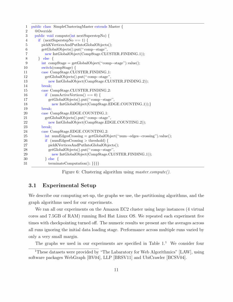
Figure 6 shows an example master.compute(), used together with the vertex-centric
computations already described (encapsulated in SimpleClusteringVertex, not shown) to
implement the overall clustering algorithm of Figure 3. Lines 2 and 3 in Figure 3 are
implemented in lines 24 and 25 of Figure 6. SimpleClusteringMaster maintains a global
object, comp-stage, that coordinates the di↵erent stages of the algorithm. Using this global
object, the master signals the vertices what stage of the algorithm they are currently in.
By looking at the value of this object, vertices know what computation to do and what
types of messages to send and receive. Thus, we are able to encapsulate vertex-centric
computations in vertex.compute(), and coordinate them globally with master.compute().
3 Static Graph Partitioning
We next present our experiments on di↵erent static partitionings of the graph. In Sec-
tion 3.2 we show that by partitioning large graphs “intelligently” before computation be-
gins, we can reduce total network I/O by up to 13.6x and run-time by up to 2.5x. The
e↵ects of partitioning depend on three factors: (1) the graph algorithm being executed; (2)
the graph itself; and (3) the configuration of the worker tasks across compute nodes. We
show experiments for a variety of settings demonstrating the importance of all three factors.
We also explore partitioning the adjacency lists of high-degree vertices across workers. We
report on those performance improvements in Section 3.4. Section 3.1 explains our experi-
mental set-up, and Section 3.3 repeats some of our experiments on the Giraph open-source
graph processing system.
10
1 public class SimpleClusteringMaster extends Master {2 @Override3 public void compute(int nextSuperstepNo) {4 if (nextSuperstepNo == 1) {5 pickKVerticesAndPutIntoGlobalObjects();6 getGlobalObjects().put(‘‘ comp�stage’’,7 new IntGlobalObject(CompStage.CLUSTER FINDING 1));8 } else {9 int compStage = getGlobalObject(‘‘comp�stage’’).value();
10 switch(compStage) {11 case CompStage.CLUSTER FINDING 1:12 getGlobalObjects().put(‘‘ comp�stage’’,13 new IntGlobalObject(CompStage.CLUSTER FINDING 2));14 break;15 case CompStage.CLUSTER FINDING 2:16 if (numActiveVertices() == 0) {17 getGlobalObjects().put(‘‘ comp�stage’’,18 new IntGlobalObject(CompStage.EDGE COUNTING 1));}19 break;20 case CompStage.EDGE COUNTING 1:21 getGlobalObjects().put(‘‘ comp�stage’’,22 new IntGlobalObject(CompStage.EDGE COUNTING 2));23 break;24 case CompStage.EDGE COUNTING 2:25 int numEdgesCrossing = getGlobalObject(‘‘num�edges�crossing’’).value();26 if (numEdgesCrossing > threshold) {27 pickKVerticesAndPutIntoGlobalObjects();28 getGlobalObjects().put(‘‘ comp�stage’’,29 new IntGlobalObject(CompStage.CLUSTER FINDING 1));30 } else {31 terminateComputation(); }}}}
Figure 6: Clustering algorithm using master.compute().
3.1 Experimental Setup
We describe our computing set-up, the graphs we use, the partitioning algorithms, and the
graph algorithms used for our experiments.
We ran all our experiments on the Amazon EC2 cluster using large instances (4 virtual
cores and 7.5GB of RAM) running Red Hat Linux OS. We repeated each experiment five
times with checkpointing turned o↵. The numeric results we present are the averages across
all runs ignoring the initial data loading stage. Performance across multiple runs varied by
only a very small margin.
The graphs we used in our experiments are specified in Table 1.1 We consider four
1These datasets were provided by “The Labaratory for Web Algorithmics” [LAW], usingsoftware packages WebGraph [BV04], LLP [BRSV11] and UbiCrawler [BCSV04].
11

Name Vertices Edges Descriptionuk-2007-d 106M 3.7B web graph of the .uk domain from 2007 (directed)uk-2007-u 106M 6.6B undirected version of uk-2007-dsk-2005-d 51M 1.9B web graph of the .sk domain from 2005 (directed)sk-2005-u 51M 3.2B undirected version of sk-2005-dtwitter-d 42M 1.5B Twitter “who is followed by who” network (directed)uk-2005-d 39M 750M web graph of the .uk domain from 2005 (directed)uk-2005-u 39M 1.5B undirected version of uk-2005-d
Table 1: Data sets.
di↵erent static partitionings of the graphs:
• Random: The default “mod” partitioning method described in Section 2, with vertex
IDs ensured to be random.
• METIS-default: METIS [MET] is publicly-available software that divides a graph into
a specified number of partitions, trying to minimize the number of edges crossing the
partitions. By default METIS balances the number of vertices in each partition. We
set the ufactor parameter to 5, resulting in at most 0.5% imbalance in the number of
vertices assigned to each partition [MET].
• METIS-balanced: Using METIS’ multi-constraint partitioning feature [MET], we gen-
erate partitions in which the number of vertices, outgoing edges, and incoming edges of
partitions are balanced. We again allow 0.5% imbalance in each of these constraints.
METIS-balanced takes more time to compute than METIS-default, although partition-
ing time itself is not a focus of our study.
• Domain-based: In this partitioning scheme for web graphs only, we locate all web pages
from the same domain in the same partition, and partition the domains randomly across
the workers.
Unless stated otherwise, we always generate the same number of partitions as we have
workers.
Note that we are assuming an environment in which partitioning occurs once, while
graph algorithms may be run many times, therefore we focus our experiments on the e↵ect
partitioning has on algorithms, not on the cost of partitioning itself.
We use four di↵erent graph algorithms in our experiments:
• PageRank (PR) [BP98]
• Finding shortest paths from a single source (SSSP), as implemented in [MAB+11]
12

• The HCC [KTF09] algorithm to find connected components
• RW-n, a pure random-walk simulation algorithm. Each vertex starts with an initial
number of n walkers. For each walker i on a vertex u, u randomly picks one of its
neighbors, say v, to simulate i’s next step. For each neighbor v of u, u sends a message
to v indicating the number of walkers that walked from u to v.
3.2 Performance E↵ects of Partitioning
Because of their bulk synchronous nature, the speed of systems like Pregel, GPS, and
Giraph is determined by the slowest worker to reach the synchronization points between
supersteps. We can break down the workload of a worker into three parts:
1. Computation: Looping through vertices and executing vertex.compute()
2. Networking: Sending and receiving messages between workers
3. Parsing and enqueuing messages: In our implementation, where messages are stored
as raw bytes, this involves byte array allocations and copying between byte arrays.
Although random partitioning generates well-balanced workloads across workers, almost
all messages are sent across the network. We show that we can both maintain a balanced
workload across workers and significantly reduce the network messages and overall run-time
by partitioning the graph using our more sophisticated schemes.
With sophisticated partitioning of the graph we can obviously reduce network I/O,
since we localize more edges within each worker compared to random partitioning. Our
first set of experiments, presented in Section 3.2.1, quantifies the network I/O reduction
for a variety of settings.
In Section 3.2.2, we present experiments measuring the run-time reduction due to so-
phisticated partitioning when running various algorithms in a variety of settings. We
observe that partitioning schemes that maintain workload balance among workers perform
better than schemes that do not, even if the latter have somewhat lower communication.
In Section 3.2.3, we discuss how to fix the workload imbalance among workers when a
partitioning scheme generates imbalanced partitions.
3.2.1 Network I/O
In our first set of experiments, we measured network I/O (network writes in GB across all
workers) when running di↵erent graph algorithms under di↵erent partitioning schemes in
13
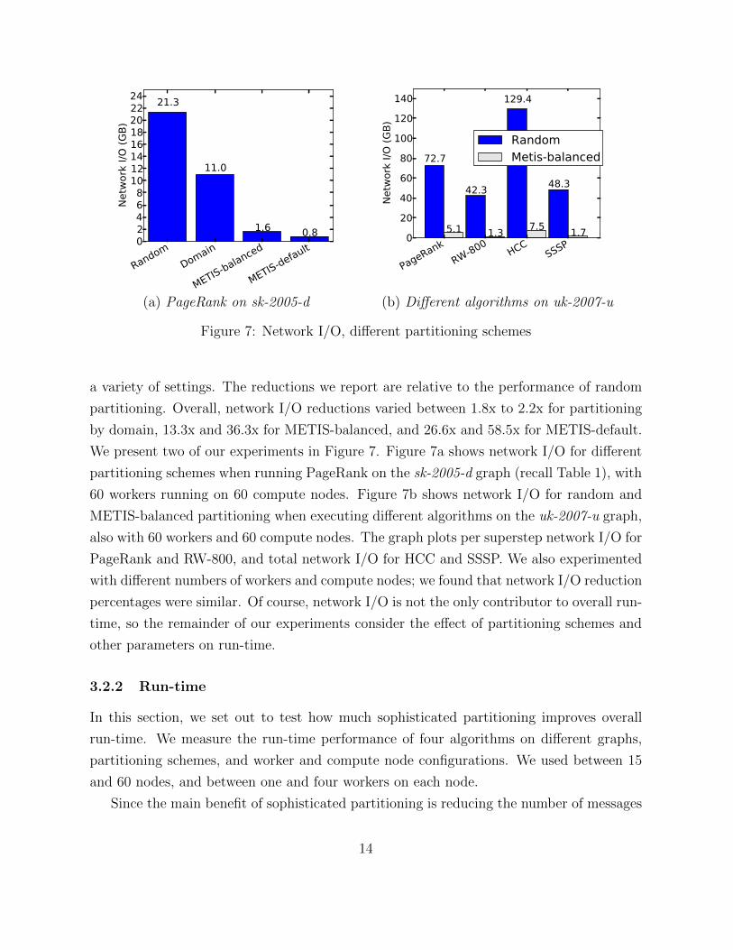
(a) PageRank on sk-2005-d (b) Di↵erent algorithms on uk-2007-u
Figure 7: Network I/O, di↵erent partitioning schemes
a variety of settings. The reductions we report are relative to the performance of random
partitioning. Overall, network I/O reductions varied between 1.8x to 2.2x for partitioning
by domain, 13.3x and 36.3x for METIS-balanced, and 26.6x and 58.5x for METIS-default.
We present two of our experiments in Figure 7. Figure 7a shows network I/O for di↵erent
partitioning schemes when running PageRank on the sk-2005-d graph (recall Table 1), with
60 workers running on 60 compute nodes. Figure 7b shows network I/O for random and
METIS-balanced partitioning when executing di↵erent algorithms on the uk-2007-u graph,
also with 60 workers and 60 compute nodes. The graph plots per superstep network I/O for
PageRank and RW-800, and total network I/O for HCC and SSSP. We also experimented
with di↵erent numbers of workers and compute nodes; we found that network I/O reduction
percentages were similar. Of course, network I/O is not the only contributor to overall run-
time, so the remainder of our experiments consider the e↵ect of partitioning schemes and
other parameters on run-time.
3.2.2 Run-time
In this section, we set out to test how much sophisticated partitioning improves overall
run-time. We measure the run-time performance of four algorithms on di↵erent graphs,
partitioning schemes, and worker and compute node configurations. We used between 15
and 60 nodes, and between one and four workers on each node.
Since the main benefit of sophisticated partitioning is reducing the number of messages
14

(a) PageRank (50 iter.) on sk-2005-d (b) Di↵erent algorithms on uk-2007-u
Figure 8: Run-time, di↵erent partitioning schemes
sent over the network, we expect partitioning to improve run-time most in algorithms that
generate a lot of messages and have low computational workloads. The computation and
communication workloads of the graph algorithms we use can be characterized as:
• PageRank: short per-vertex computation, high communication
• HCC: short per-vertex computation, medium communication
• RW-800: long per-vertex computation (due to random number generation), medium
communication
• SSSP: short per-vertex computation, low communication
A sample of our experimental results is shown in Figure 8. Figure 8a shows PageRank
on the sk-2005-d graph on 60 compute nodes with 60 workers. In this experiment, improve-
ments ranged between 1.1x for domain-based partitioning to 2.3x for METIS-balanced. In
other experiments for PageRank, METIS-balanced consistently performed best, reducing
run-time between 2.1x to 2.5x over random partitioning. Improvements for METIS-default
varied from 1.4x to 2.4x and for domain-based partitioning from 1.1x to 1.7x.
Run-time reductions when executing other graph algorithms are less than PageRank,
which is not surprising since PageRank has the highest communication to computation
ratio of the algorithms we consider. Figure 8b shows four algorithms on the uk-2007-u
graph using 30 workers running on 30 compute nodes. We compared the performance of
random partitioning and METIS-balanced. As shown, METIS-balanced reduces the run-
15

Figure 9: Slowest worker, number of messages.
time by 2.2x when executing PageRank, and by 1.47x, 1.08x, and 1.06x for HCC, SSSP,
and RW-800, respectively.
3.2.3 Workload Balance
In all of our experiments reported so far, METIS-default performed better than METIS-
balanced in network I/O but worse in run-time. The reason for this counterintuitive perfor-
mance is that METIS-default tends to create bottleneck workers that slow down the system.
For all of the graph algorithms we are considering, messages are sent along the edges. Re-
call that METIS-default balances only the number of vertices in each partition and not the
edges. As a result, some workers process a significantly higher number of messages than
average. Figure 9 shows the number of messages processed by the slowest workers in each
of the experiments of Figure 8a. The message counts for Random and METIS-balanced
indicate fairly homogeneous workloads (perfect distribution would be about 63M messages
per worker). But with METIS-default, one partition has more than twice the average load
of other partitions, thus slowing down the entire system.
We discuss how to improve workload imbalance, and in turn improve the run-time
benefits when using a sophisticated partitioning scheme that can generate imbalanced par-
titions. One approach is to generate more partitions than we have workers, then assign
multiple partitions to each worker, thus averaging the workloads from “heavy” and “light”
16
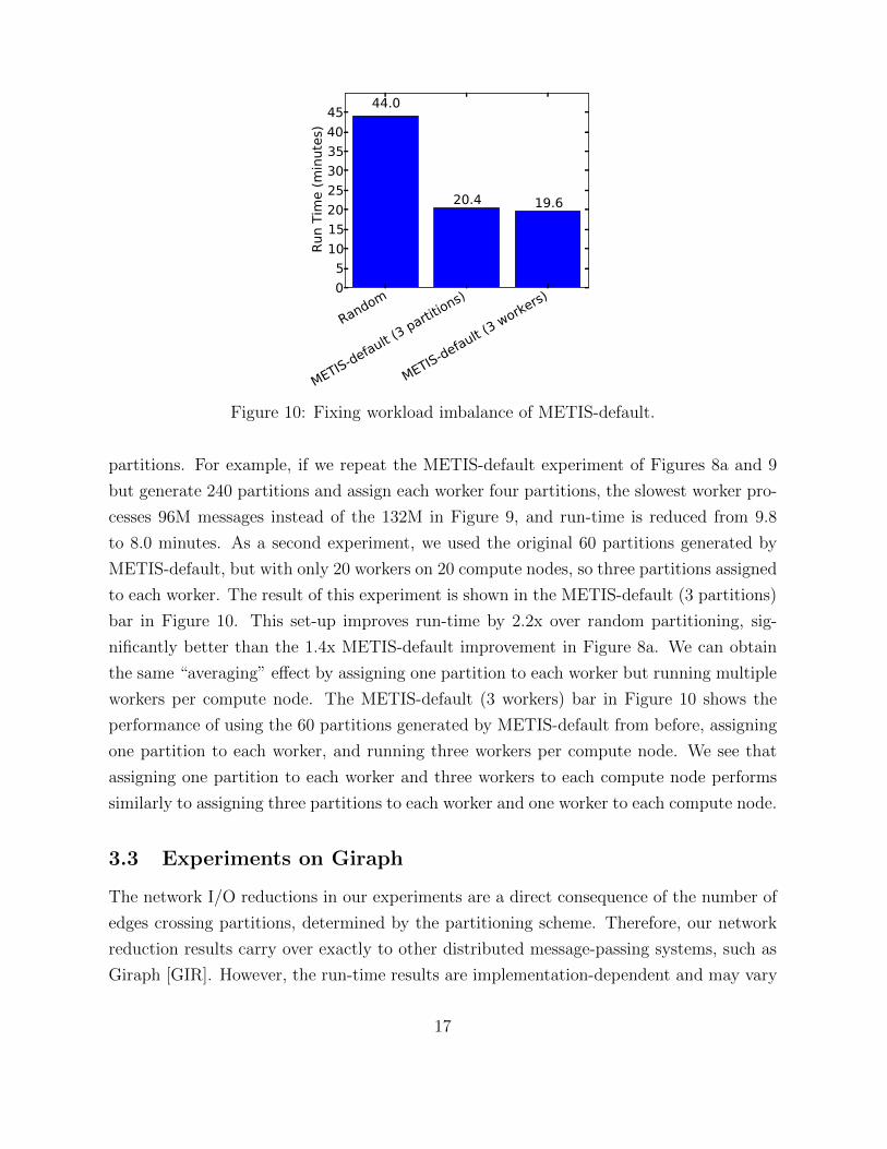
Figure 10: Fixing workload imbalance of METIS-default.
partitions. For example, if we repeat the METIS-default experiment of Figures 8a and 9
but generate 240 partitions and assign each worker four partitions, the slowest worker pro-
cesses 96M messages instead of the 132M in Figure 9, and run-time is reduced from 9.8
to 8.0 minutes. As a second experiment, we used the original 60 partitions generated by
METIS-default, but with only 20 workers on 20 compute nodes, so three partitions assigned
to each worker. The result of this experiment is shown in the METIS-default (3 partitions)
bar in Figure 10. This set-up improves run-time by 2.2x over random partitioning, sig-
nificantly better than the 1.4x METIS-default improvement in Figure 8a. We can obtain
the same “averaging” e↵ect by assigning one partition to each worker but running multiple
workers per compute node. The METIS-default (3 workers) bar in Figure 10 shows the
performance of using the 60 partitions generated by METIS-default from before, assigning
one partition to each worker, and running three workers per compute node. We see that
assigning one partition to each worker and three workers to each compute node performs
similarly to assigning three partitions to each worker and one worker to each compute node.
3.3 Experiments on Giraph
The network I/O reductions in our experiments are a direct consequence of the number of
edges crossing partitions, determined by the partitioning scheme. Therefore, our network
reduction results carry over exactly to other distributed message-passing systems, such as
Giraph [GIR]. However, the run-time results are implementation-dependent and may vary
17

Figure 11: Experiments on Giraph [GIR].
from system to system. To test whether sophisticated partitioning of graphs can improve
run-time in other systems, we repeated some of our experiments in Giraph. Figure 11
summarizes our results. METIS-balanced yields 1.6x run-time improvement over random
partitioning for PageRank. Similar to our results in GPS, the improvements are less for
SSSP and HCC. We also note that GPS runs ⇠12x faster than Giraph on the same ex-
periments. We explain the main implementation di↵erences between Giraph and GPS in
Section 5.
3.4 Large Adjacency-List Partitioning
GPS includes an optimization called LALP (large adjacency list partitioning), in which
adjacency lists of high-degree vertices are not stored in a single worker, but rather are
partitioned across workers. This optimization can improve performance, but only for algo-
rithms with two properties: (1) Vertices use their adjacency lists (outgoing neighbors) only
to send messages and not for computation; (2) If a vertex sends a message, it sends the
same message to all of its outgoing neighbors. For example, in PageRank each vertex sends
its latest PageRank value to all of its neighbors, and that is the only time vertices access
their adjacency lists. On the other hand, RW-n does not satisfy property 2: a message
from vertex u to its neighbor v contains the number of walkers that move from u to v and
is not necessarily the same as the message u sends to its other neighbors.
Suppose a vertex u is located in worker Wi and let Nj(u) be the outgoing neighbors of
u located in worker Wj. Suppose |Nj(u)| = 10000. During the execution of PageRank, Wi
sends 10000 copies of the same message to Wj in each superstep, one for each vertex in
Nj(u). Instead, if Wj stores Nj(u), Wi need send only a single message to Wj for node u,
18
(a) Network I/O (b) Total run-time
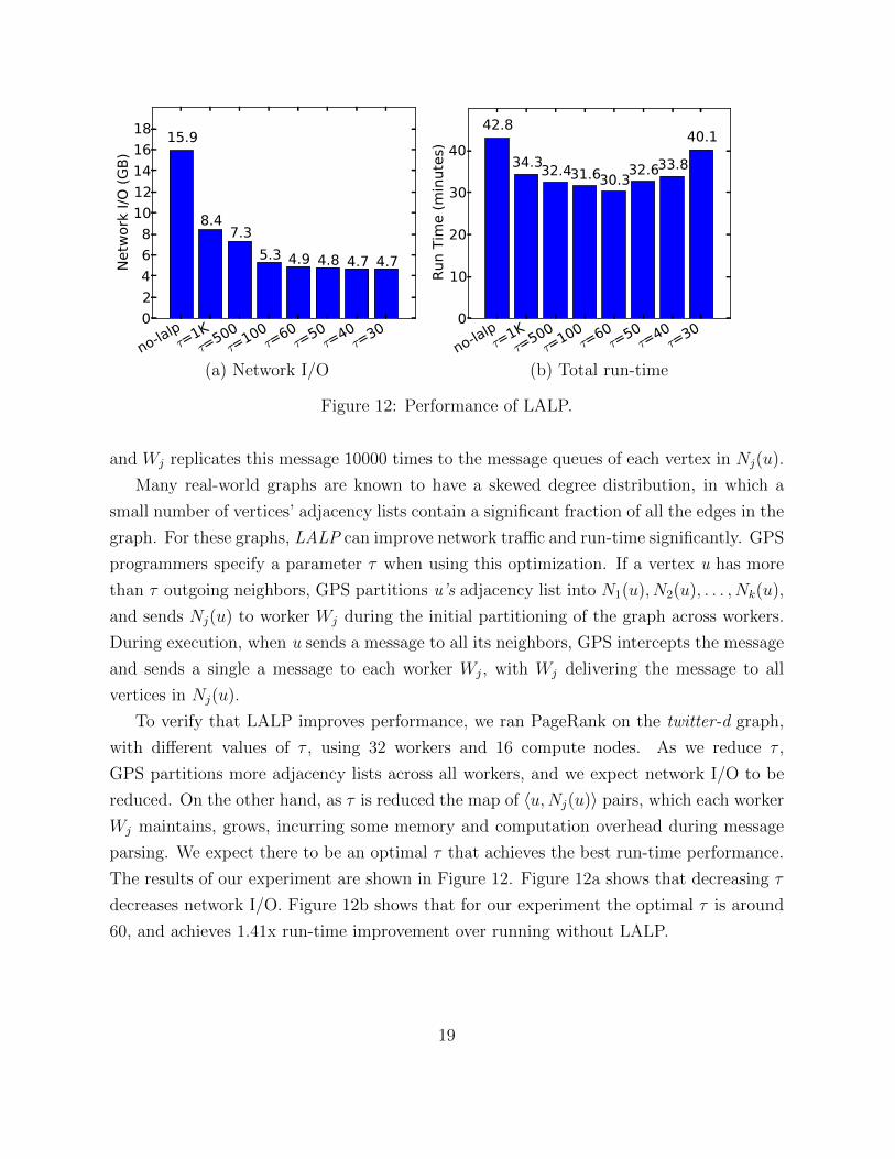
Figure 12: Performance of LALP.
and Wj replicates this message 10000 times to the message queues of each vertex in Nj(u).
Many real-world graphs are known to have a skewed degree distribution, in which a
small number of vertices’ adjacency lists contain a significant fraction of all the edges in the
graph. For these graphs, LALP can improve network tra�c and run-time significantly. GPS
programmers specify a parameter ⌧ when using this optimization. If a vertex u has more
than ⌧ outgoing neighbors, GPS partitions u’s adjacency list into N
1
(u), N2
(u), . . . , Nk(u),
and sends Nj(u) to worker Wj during the initial partitioning of the graph across workers.
During execution, when u sends a message to all its neighbors, GPS intercepts the message
and sends a single a message to each worker Wj, with Wj delivering the message to all
vertices in Nj(u).
To verify that LALP improves performance, we ran PageRank on the twitter-d graph,
with di↵erent values of ⌧ , using 32 workers and 16 compute nodes. As we reduce ⌧ ,
GPS partitions more adjacency lists across all workers, and we expect network I/O to be
reduced. On the other hand, as ⌧ is reduced the map of hu,Nj(u)i pairs, which each worker
Wj maintains, grows, incurring some memory and computation overhead during message
parsing. We expect there to be an optimal ⌧ that achieves the best run-time performance.
The results of our experiment are shown in Figure 12. Figure 12a shows that decreasing ⌧
decreases network I/O. Figure 12b shows that for our experiment the optimal ⌧ is around
60, and achieves 1.41x run-time improvement over running without LALP.
19

4 Dynamic Repartitioning
To reduce the number of messages sent over the network, it might be helpful to reassign
certain vertices to other workers dynamically during algorithm computation. There are
three questions any dynamic repartitioning scheme must answer: (1) which vertices to
reassign; (2) how and when to move the reassigned vertices to their new workers; (3)
how to locate the reassigned vertices. Below, we explain our answers to these questions
in GPS and discuss other possible options. We also present experiments measuring the
network I/O and run-time performance of GPS when the graph is initially partitioned by
one of our partitioning schemes from Section 3, then dynamically repartitioned during the
computation.
4.1 Picking Vertices to Reassign
One option is to reassign vertex u at worker Wi to a new worker Wj if u send/receives more
message to/from Wj than to/from any other worker, and that number of messages is over
some threshold. There are two issues with this approach. First, in order to observe incoming
messages, we need to include the source worker in each message, which can increase the
memory requirement significantly when the size of the actual messages are small. To avoid
this memory requirement, GPS bases reassignment on sent messages only.
Second, using this basic reassignment technique, we observed that over multiple itera-
tions, more and more vertices were reassigned to only a few workers, creating significant
imbalance. Despite the network benefits, the “dense” workers significantly slowed down
the system. To maintain balance, GPS exchanges vertices between workers. Each worker
Wi constructs a set Sij of vertices that potentially will be reassigned to Wj, for each Wj.
Similarly Wj constructs a set Sji. Then Wi and Wj communicate the sizes of their sets and
exchange exactly min(Sij, Sji) vertices, guaranteeing that the number of vertices in each
worker does not change through dynamic repartitioning.
4.2 Moving Reassigned Vertices to New Workers
Once a dynamic partitioning scheme decides to reassign a vertex u from Wi to Wj in
superstep x, three pieces of data associated with u must be sent to Wj: (a) u’s latest value;
(b) u’s adjacency list; and (c) u’s messages for superstep (x+ 1). One option is to insert a
“vertex moving” stage between the end of superstep x and beginning of superstep x + 1,
during which all vertex data is moved. GPS uses another option that combines vertex
20

moving within the supersteps themselves: At the end of superstep x, workers exchange
their set sizes as described in the previous subsection. Then, between the end of superstep
x and beginning of superstep (x + 1), the exact vertices to be exchanged are determined
and the adjacency lists are relabeled, as described in the next subsection. Relabeling of the
adjacency lists ensures that all messages that will be sent to u in superstep x+ 1 are sent
to Wj. However, u is not sent to Wj at this point. During the computation of superstep
(x + 1), Wi first calls u.compute() and then sends only u’s adjacency list and latest value
to Wj. Thus, u’s messages for superstep (x+ 1) are not sent to Wj, reducing the network
overhead of dynamic repartitioning.
4.3 Locating Reassigned Vertices
When a vertex u gets reassigned to a new worker, every worker in the cluster must obtain
and store this information in order to deliver future messages to u. An obvious option
is for each worker to store an in-memory map consisting of <vertex-id, new-worker-id>
pairs. Of course, over time, this map can potentially contain as many pairs as there are
vertices in the original graph, causing a significant memory and computation bottleneck.
In our experiments, up to 90% of vertices can eventually get reassigned. Thus, GPS instead
uses an approach based on relabeling the IDs of reassigned vertices. Suppose u has been
reassigned to Wj. We give u a new ID u
0, such that (u0 mod k) = j. Since every pair
Wi and Wj exchange the same number of vertices, vertex IDs can e↵ectively be exchanged
as well. In addition, each worker must go through all adjacency lists in its partition and
change each occurrence of u to u
0.
There are two considerations in this approach:
• If the application requires the original node IDs to be output at the end of the compu-
tation, this information must be retained with nodes whose IDs are modified, incurring
some additional storage.
• When a node u is relabeled with a new ID, we modify its ID in the adjacency lists of all
nodes with an edge to u. If the graph algorithm being executed involves messages not
following edges (that is, messages from a node u
1
to a node u
2
where there is no edge
from u
1
to u
2
), then our relabeling scheme cannot be used. In most graph algorithms
suitable for GPS, messages do follow edges.
21

(a) Network I/O
(b) Run-time
Figure 13: Performance of PageRank with and without dynamic repartitioning.
4.4 Dynamic Repartitioning Experiments
Dynamic repartitioning is intended to improve network I/O and run-time by reducing the
number of messages sent over the network. On the other hand, dynamic repartitioning
also incurs network I/O overhead by sending vertex data between workers, and run-time
overhead deciding which vertices to send and relabeling adjacency lists. It would not be
surprising if, in the initial supersteps of an algorithm using dynamic repartitioning, the
overhead exceeds the benefits. We expect that there is a crossover superstep s, such that
dynamic repartitioning performs better than static partitioning only if the graph algorithm
runs for more than s supersteps. Obviously, s could be di↵erent for network I/O versus
run-time performance, and depends on the graph, graph algorithm, and initial partitioning.
In our first experiment, we ran PageRank on the uk-2007-d graph for between 3 and 100
iterations, with random initial partitioning, and with and without dynamic repartitioning.
22

We used 30 workers running on 30 compute nodes. In GPS, the master task turns dy-
namic repartitioning o↵ when the number of vertices being exchanged is below a threshold,
which is by default 0.1% of the total number of vertices in the graph. In our PageRank
experiments, this typically occurred around superstep 15-20. Our results are shown in
Figure 13. The crossover superstep in this experiment was five iterations for network I/O
and around 55 iterations for run-time. When running PageRank for long enough, dynamic
repartitioning gives 2.0x performance improvement for network I/O and 1.13x for run-time.
We repeated our experiment, now initially partitioning the graph using METIS-balanced
and domain-based, rather than random. When the initial partitioning is METIS-balanced,
we do not see noticeable network I/O or run-time benefits from dynamic repartitioning. On
the other hand, when we start with domain-based partitioning, the crossover iteration is 4
for network I/O and 36 for run-time. When running PageRank for long enough, dynamic
repartitioning shows 2.2x and 1.2x performance improvement for network I/O and run-time,
respectively.
In our setting, the run-time benefits of dynamic repartitioning seem to be modest at
best. However, in settings where networking is slower, benefits from network I/O should
yield significant run-time improvements as well.
5 Other System Optimizations
We describe several optimizations in GPS that reduce memory usage and increase overall
performance.
• Combining messages at the receiver worker: Combiners were introduced in the
MapReduce framework to reduce the number of intermediate values sent from Mappers
to Reducers [DG04], when the Reducers use these values in commutative and associative
operations. Similarly, Pregel [MAB+11] uses combiners at the sender and receiver
workers to reduce both the number of messages sent between workers and the memory
required to store messages in each worker. At the sender sider, when multiple vertices
from worker Wi send messages to a vertex v located in Wj, Wi can combine some of
these messages at certain intervals and send fewer messages to Wj, reducing network
I/O. At the receiver side, when a message m is received in Wj for v, if the message
list for v is empty, Wj can add m to v’s message list. Otherwise, instead of appending
m to the list, Wj can immediately combine its value with the current message in the
list. Receiver-side combining reduces the total memory required to store messages for a
23
particular superstep from |E| to |V |—a significant reduction in most graphs where the
number of edges is significantly higher than the number of vertices.
GPS supports only receiver-side combining. In earlier versions of GPS, we implemented
sender-side combining. In order to combine messages at a sender worker Wi, Wi needs
to store an outgoing message list for each vertex v that receives a message from Wi,
which increases memory usage. Also, messages are bu↵ered twice, once in the outgoing
messages lists, and then in the message bu↵ers for each worker, which slows down
the rate at which bu↵ers fill and are flushed. Overall, we did not observe significant
performance improvements by combining messages at the sender.
• Single Vertex and Message objects: GPS reduces the memory cost of allocating
many Java objects by storing canonical objects. First, instead of storing the value
and the adjacency list of each vertex v inside a separate Vertex object, and calling
vertex.compute() on each object as in Giraph, GPS workers use a single canonical Vertex
object, with vertex values and adjacency lists stored in separate data structures. For
each vertex v in worker Wi, Wi is configured so the canonical Vertex object has access
to v’s value and adjacency list. Wi then calls vertex.compute() on the canonical object.
Similarly, GPS workers store a single canonical Message object. Incoming messages
are stored as raw bytes in the message queues, and a message is deserialized into the
canonical Message object only when the canonical Vertex object iterates over it.
• Controlling the speed of message generation: Recall from Section 2 that the
computation thread generates and bu↵ers outgoing messages by calling vertex.com-
pute() on active vertices. When an outgoing message bu↵er is full, the computation
thread gives it to networking threads to send over the network. We have observed
that we can significantly improve the overall speed of GPS by controlling the speed of
message generation and limiting the number of bu↵ers that are being sent concurrently
over the network. GPS controls these factors in two ways. First, at certain intervals,
the computation thread checks the number of bu↵ers it has given to the networking
layer. If the number is above a threshold (two, by default), the computation thread
waits. Second, the networking threads send only a fixed number of the outgoing bu↵ers
concurrently over the network (again two, by default). These controls save memory and
improve network speed, leading to improved overall performance.
As we showed in Section 3, GPS is ⇠12 times faster than Giraph on the graphs and
algorithms we tried. In addition to our optimizations above, we believe there are two more
implementation di↵erences between GPS and Giraph that explain this di↵erential:
24
1. Message Bu↵ers: Giraph organizes its message buffers per vertex rather than per
worker. Both Giraph and GPS wait until bu↵ers are full to send them, or until the
end of the superstep when bu↵ers are flushed. Per-vertex bu↵ers take much longer
to fill, delaying overall network speed.
2. Synchronization: As explained in Section 2, GPS threads synchronize only for each
sent and received message bu↵er. In Giraph, the RPC calls from di↵erent workers to
a particular worker Wi synchronize with each other, as they access the same message
queues in Wi. Therefore, there is possible synchronization between threads for each
message received by a worker, which is much more frequent than synchronizing per
message bu↵er.
The system optimizations described in this section have been key to the high perfor-
mance of GPS; we hope to integrate some of them into Giraph.
6 Related Work
There are several classes of systems designed to do large-scale graph computations:
• Bulk synchronous message-passing systems: Pregel [MAB+11] introduced the
first bulk synchronous distributed message-passing system, which GPS has drawn from.
Several other systems are based on Pregel, including Giraph [GIR], GoldenOrb [GOL],
Phoebus [PHO], Hama [HAM], JPregel [JPR] and Bagel [BAG] . Giraph is the most
popular and advanced of these systems. Giraph jobs run as Hadoop jobs without the
reduce phase. Giraph leverages the task scheduling component of Hadoop clusters
by running workers as special mappers, that communicate with each other to deliver
messages between vertices and synchronize in between supersteps.
• Hadoop-based systems: Many graph algorithms, e.g., computing PageRank or find-
ing connected components, are iterative computations that terminate when a vertex-
centric convergence criterion is met. Because MapReduce is a two-phased computational
model, these graph algorithms cannot be expressed in Hadoop easily. One approach
to solve this limitation has been to build systems on top of Hadoop, in which the
programmer can express a graph algorithm as a series of MapReduce jobs, each one
corresponding to one iteration of the algorithm. Pegasus [KTF09], Mahout [MAH],
HaLoop [BHBE10], iMapReduce [ZGGW11], Surfer [CWHY10] and Twister [ELZ+10]
are examples of these systems. These systems su↵er from two ine�ciencies that do not
25

exist in bulk synchronous message-passing systems: (1) The input graph, which does
not change from iteration to iteration, may not stay in RAM, and is sent from mappers
to reducers in each iteration. (2) Checking for the convergence criterion may require
additional MapReduce jobs.
• Asynchronous systems: GPS supports only bulk synchronous graph processing.
GraphLab [LGK+10] and Signal-Collect [SBC10] support asynchronous vertex-centric
graph processing. An advantage of asynchronous computation over bulk synchronous
computation is that fast workers do not have to wait for slow workers. However, pro-
gramming in the asynchronous model can be harder than synchronous models, as pro-
grammers have to reason about the non-deterministic order of vertex-centric function
calls. Signal-Collect also supports bulk synchronous processing, but is not a distributed
system; its parallelism is due to multithreading.
• Message Passing Interface (MPI): MPI is a standard interface for building a broad
range of message passing programs. There are several implementations of MPI [OPE,
MPI, PYM, OCA], which can be used to implement parallel message-passing graph
algorithms in various programming languages. MPI consists of very low-level communi-
cation primitives that do not provide any consistency or fault-tolerance. Programmers
must build another level of abstraction (e.g., bulk synchronous consistency) on their
own, which makes programming harder than bulk synchronous message-passing sys-
tems.
• Other systems: HipG [KKFB10] is a system in which each vertex is a Java object
and the computation is done sequentially starting from a particular vertex. The code
is expressed as if the graph is in a single machine, and the reads and writes to vertices
residing in other machines are translated as RPC calls. HipG incurs significant overhead
from RPC calls when executing algorithms, such as PageRank, that compute a value for
each vertex in the graph. Spark [ZCF+10] is a general cluster computing system, whose
API is designed to express generic iterative computations. As a result, programming
graph algorithms on Spark requires significant more coding e↵ort than on GPS.
In addition to presenting GPS, we studied the e↵ects of di↵erent graph partitioning
schemes on the performance of GPS when running di↵erent graph algorithms. We also stud-
ied the e↵ects of GPS’s dynamic repartitioning scheme on performance. There are previ-
ous studies on the performance e↵ects of di↵erent partitionings of graphs on other systems.
[HAR11] shows that by partitioning Resource Description Framework [RDF04] (RDF) data
with METIS and then “intelligently” replicating certain tuples, SPARQL [SPA06] query
26

run-times can be improved significantly over random partitioning. We study the e↵ects of
partitioning under batch algorithms, whereas SPARQL queries consist of short path-finding
workloads. [SK11] develops a heuristic to partition the graph across machines during the
initial loading phase. They study the reduction in the number of edges crossing machines
and run-time improvements on Spark when running PageRank. They do not study the
e↵ects of other static or dynamic partitioning schemes.
7 Conclusions and Future Work
We presented GPS, an open source distributed message-passing system for large-scale graph
computations. Like Pregel [MAB+11] and Giraph [GIR], GPS is designed to be scalable,
fault-tolerant, and easy to program through simple user-provided functions. Using GPS,
we studied the network and run-time e↵ects of di↵erent graph partitioning schemes in a
variety of settings. We also described GPS’s dynamic repartitioning feature, and presented
several other system optimizations that increase the performance of GPS.
As future work, we are interested in exploring which graph algorithms are suitable
for running on systems like GPS and Pregel. On the theoretical side, we want to un-
derstand exactly which graph algorithms can be implemented e�ciently using bulk syn-
chronous processing and message-passing between vertices. For example, although there
are bulk synchronous message-passing algorithms to find the weakly connected components
of undirected graphs, we do not know of any such algorithm for finding strongly connected
components.
On the practical side, we want to o↵er a higher-level programming interface as an alter-
native to implementing bulk synchronous message-passing algorithms directly. An analogy
would be the Pig [ORS+08] and Hive [TSJ+09] languages implemented on top of Hadoop.
As a first step in this direction, we are working on compiling Green-Marl [HCSO12], a
domain-specific language for graph algorithms, into GPS.
8 Acknowledgements
We are grateful to Sungpack Hong, Jure Leskovec, and Hyunjung Park for numerous useful
discussions.
27

References
[BAG] Bagel Programming Guide. https://github.com/mesos/spark/wiki/Bagel-
Programming-Guide/.
[BCSV04] Paolo Boldi, Bruno Codenotti, Massimo Santini, and Sebastiano Vigna. Ub-
iCrawler: A Scalable Fully Distributed Web Crawler. Software: Practice &
Experience, 34(8):711–726, 2004.
[BHBE10] Yingyi Bu, Bill Howe, Magdalena Balazinska, and Michael D. Ernst. HaLoop:
E�cient iterative data processing on large clusters. Proceedings of the Inter-
national Conference on Very Large Databases, pages 285–296, 2010.
[BP98] Sergey Brin and Lawrence Page. The Anatomy of Large-Scale Hypertextual
Web Search Engine. In Proceedings of the International Conference on The
World Wide Web, pages 107–117, 1998.
[BRSV11] Paolo Boldi, Marco Rosa, Massimo Santini, and Sebastiano Vigna. Layered
Label Propagation: A MultiResolution Coordinate-Free Ordering for Com-
pressing Social Networks. In Proceedings of the 20th international conference
on World Wide Web. ACM Press, 2011.
[BV04] Paolo Boldi and Sebastiano Vigna. The WebGraph framework I: Compression
techniques. In Proc. of the Thirteenth International World Wide Web Confer-
ence (WWW 2004), pages 595–601, Manhattan, USA, 2004. ACM Press.
[CWHY10] R. Chen, X. Weng, B. He, and M. Yang. Large graph processing in the cloud.
In Proceedings of the International Conference on Management of Data, pages
1123–1126, 2010.
[DG04] Je↵rey Dean and Sanjay Ghemawat. MapReduce: Simplified data processing
on large clusters. In Proceedings of the Symposium on Operating System Design
and Implementation, pages 137–150, 2004.
[ELZ+10] Jaliya Ekanayake, Hui Li, Bingjing Zhang, Thilina Gunarathne, Seung-Hee
Bae, Judy Qiu, and Geo↵rey Fox. Twister: a runtime for iterative mapreduce.
In Proceedings of the 19th ACM International Symposium on High Performance
Distributed Computing, HPDC ’10, pages 810–818, New York, NY, USA, 2010.
ACM.
28

[GIR] Apache Incubator Giraph. http://incubator.apache.org/giraph//.
[GOL] GoldenOrb. http://www.raveldata.com/goldenorb/.
[HAD] Apache Hadoop. http://hadoop.apache.org/.
[HAM] Apache Hama. http://incubator.apache.org/hama/.
[HAR11] Jiewen Huang, Daniel J. Abadi, and Kun Ren. Scalable SPARQL Querying of
Large RDF Graphs. PVLDB, 4(21), August 2011.
[HCSO12] Sungpack Hong, Hassan Chafi, Eric Sedlar, and Kunle Olukotun. Green-marl:
a dsl for easy and e�cient graph analysis. In Proceedings of the 17th Inter-
national Conference on Architectural Support for Programming Languages and
Operating Systems, pages 349–362. ACM, 2012.
[HDF] Hadoop Distributed File System. http://hadoop.apache.org/hdfs/.
[JPR] JPregel. http://kowshik.github.com/JPregel/.
[KKFB10] E. Krepska, T. Kielmann, W. Fokkink, and H. Bal. A high-level framework for
distributed processing of large-scale graphs. In Proceedings of the International
Conference on Distributed Computing and Networking, pages 1123–1126, 2010.
[KTF09] U. Kang, C. E. Tsourakakis, and C. Faloutsos. PEGASUS: A peta-scale graph
mining system – Implementation and observations. In In Proceedings of the
IEEE International Conference on Data Mining, pages 229–238, 2009.
[LAW] The Laboratory for Web Algorithmics. http://law.dsi.unimi.it/datasets.php.
[LGK+10] Yucheng Low, Joseph Gonzalez, Aapo Kyrola, Danny Bickson, Carlos
Guestrin, and Joseph M. Hellerstein. GraphLab: A New Framework for Par-
allel Machine Learning. CoRR, abs/1006.4990, 2010.
[MAB+11] Grzegorz Malewicz, Matthew H. Austern, Aart J. C. Bik, James C. Dehnert,
Ilan Horn, Naty Leiser, and Grzegorz Czajkowski. Pregel: A System for Large-
Scale Graph Processing. In Proceedings of the ACM SIGMOD International
Conference on Management of Data, pages 155–166, 2011.
[MAH] Apache Mahout. http://mahout.apache.org/.
29

[MET] METIS Graph Partition Library. http://exoplanet.eu/catalog.php.
[MPI] MPICH2. http://www.mcs.anl.gov/research/projects/mpich2/.
[OCA] OCaml MPI. http://forge.ocamlcore.org/projects/ocamlmpi/.
[OPE] Open MPI. http://www.open-mpi.org/.
[ORS+08] Christopher Olston, Benjamin Reed, Utkarsh Srivastava, Ravi Kumar, and
Andrew Tomkins. Pig latin: a not-so-foreign language for data processing.
In Proceedings of the 2008 ACM SIGMOD international conference on Man-
agement of data, SIGMOD ’08, pages 1099–1110, New York, NY, USA, 2008.
ACM.
[PHO] Phoebus. https://github.com/xslogic/phoebus.
[PYM] pyMPI. http://pympi.sourceforge.net/.
[RDF04] RDF Primer. W3C Recommendation. http://www.w3.org/TR/rdf-primer,
2004.
[SBC10] P Stutz, A Bernstein, and W W Cohen. Signal/Collect: graph algorithms for
the (Semantic) Web. In ISWC 2010, 2010.
[SK11] Isabelle Stanton and Gabriel Kliot. Streaming Graph Partitioning for Large
Distributed Graphs. Technical report, Microsoft Research Lab, November 2011.
[SPA06] SPARQL Query Language for RDF. W3C Working Draft 4.
http://www.w3.org/TR/rdf-sparql-query/, October 2006.
[TSJ+09] Ashish Thusoo, Joydeep Sen Sarma, Namit Jain, Zheng Shao, Prasad Chakka,
Suresh Anthony, Hao Liu, Pete Wycko↵, and Raghotham Murthy. Hive- A
Warehousing Solution Over a Map-Reduce Framework. In IN VLDB ’09: PRO-
CEEDINGS OF THE VLDB ENDOWMENT, pages 1626–1629, 2009.
[Val90] Leslie G. Valiant. A bridging model for parallel computation. Communications
of the ACM, 33(8):103–111, August 1990.
[ZCF+10] Matei Zaharia, Mosharaf Chowdhury, Michael J. Franklin, Scott Shenker, and
Ion Stoica. Spark: cluster computing with working sets. In Proceedings of the
30

2nd USENIX conference on Hot topics in cloud computing, HotCloud’10, pages
10–10, Berkeley, CA, USA, 2010. USENIX Association.
[ZGGW11] Y. Zhang, Q. Gao, L. Gao, and C. Wang. iMapreduce: A distributed computing
framework for iterative computation. DataCloud, 2011.
[”ZM] Apache MINA. http://mina.apache.org/.
31