GPR Data Acquisition and Interpretation

Mezgeen Rasol

PhD Candidate

Geophysics and Seismic Engineering

Polytechnic University of Catalonia

mezgeen.rasol@upc.edu

BIG-SKY-EARTH Cost Action TD1403 Workshop

Novi Sad, SerbiaFebruary 26th-27th, 2018

1

Copyrights © 2018 by Mezgeen Rasol

GPR Introduction

GPR Concept

GPR Applications

1st case study

2nd case study Outlines

2

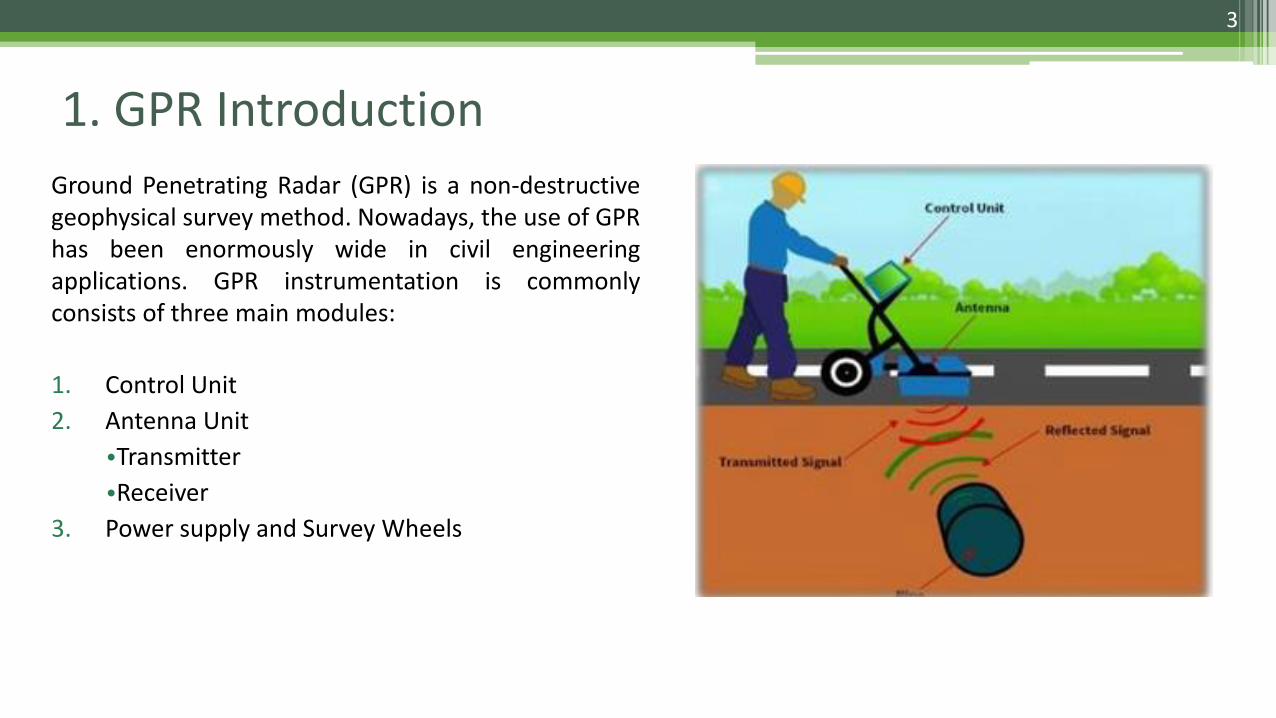
1. GPR Introduction

Ground Penetrating Radar (GPR) is a non-destructivegeophysical survey method. Nowadays, the use of GPRhas been enormously wide in civil engineeringapplications. GPR instrumentation is commonlyconsists of three main modules:

1. Control Unit

2. Antenna Unit

•Transmitter

•Receiver

3. Power supply and Survey Wheels

3

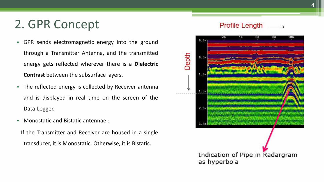
• GPR sends electromagnetic energy into the ground

through a Transmitter Antenna, and the transmitted

energy gets reflected wherever there is a Dielectric

Contrast between the subsurface layers.

• The reflected energy is collected by Receiver antenna

and is displayed in real time on the screen of the

Data-Logger.

• Monostatic and Bistatic antennae :

If the Transmitter and Receiver are housed in a single

transducer, it is Monostatic. Otherwise, it is Bistatic.

2. GPR Concept

Silty sandSand stone

Marine ss

Clay

Limestone

Shale

Limestone

Pipe

4

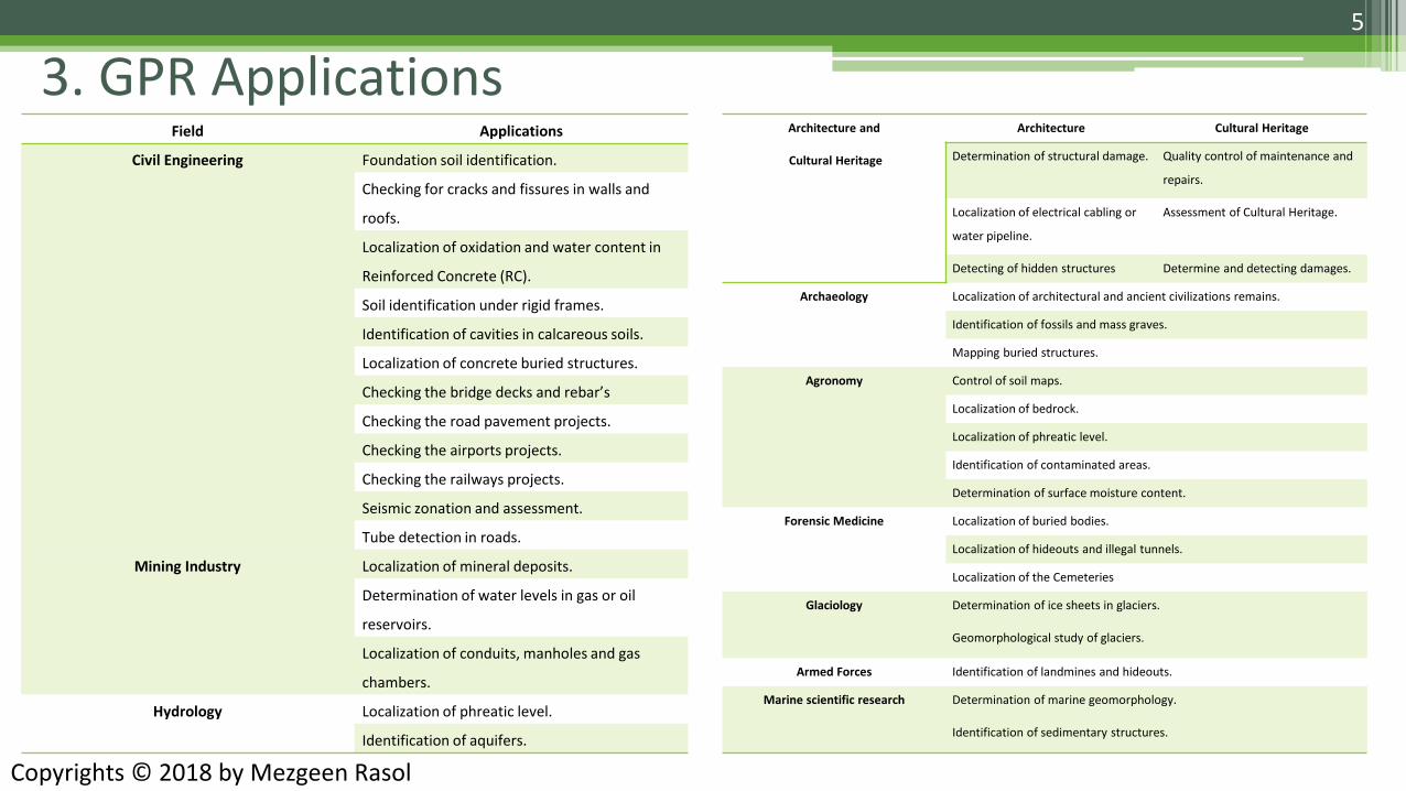
Field Applications

Civil Engineering Foundation soil identification.

Checking for cracks and fissures in walls and

roofs.

Localization of oxidation and water content in

Reinforced Concrete (RC).

Soil identification under rigid frames.

Identification of cavities in calcareous soils.

Localization of concrete buried structures.

Checking the bridge decks and rebar’s

Checking the road pavement projects.

Checking the airports projects.

Checking the railways projects.

Seismic zonation and assessment.

Tube detection in roads.

Mining Industry Localization of mineral deposits.

Determination of water levels in gas or oil

reservoirs.

Localization of conduits, manholes and gas

chambers.

Hydrology Localization of phreatic level.

Identification of aquifers.

Architecture and

Cultural Heritage

Architecture Cultural Heritage

Determination of structural damage. Quality control of maintenance and

repairs.

Localization of electrical cabling or

water pipeline.

Assessment of Cultural Heritage.

Detecting of hidden structures Determine and detecting damages.

Archaeology Localization of architectural and ancient civilizations remains.

Identification of fossils and mass graves.

Mapping buried structures.

Agronomy Control of soil maps.

Localization of bedrock.

Localization of phreatic level.

Identification of contaminated areas.

Determination of surface moisture content.

Forensic Medicine Localization of buried bodies.

Localization of hideouts and illegal tunnels.

Localization of the Cemeteries

Glaciology Determination of ice sheets in glaciers.

Geomorphological study of glaciers.

Armed Forces Identification of landmines and hideouts.

Marine scientific research Determination of marine geomorphology.

Identification of sedimentary structures.

3. GPR Applications 5

Copyrights © 2018 by Mezgeen Rasol

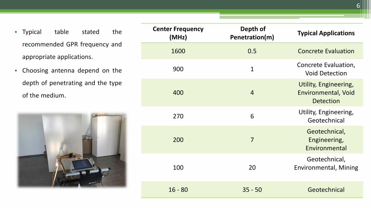
Center Frequency (MHz)

Depth of Penetration(m)

Typical Applications

1600 0.5 Concrete Evaluation

900 1Concrete Evaluation,

Void Detection

400 4Utility, Engineering, Environmental, Void

Detection

270 6Utility, Engineering,

Geotechnical

200 7Geotechnical, Engineering,

Environmental

100 20Geotechnical,

Environmental, Mining

16 - 80 35 - 50 Geotechnical

• Typical table stated the

recommended GPR frequency and

appropriate applications.

• Choosing antenna depend on the

depth of penetrating and the type

of the medium.

6

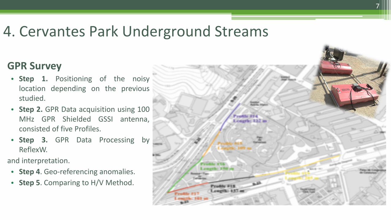
4. Cervantes Park Underground Streams

GPR Survey• Step 1. Positioning of the noisy

location depending on the previousstudied.

• Step 2. GPR Data acquisition using 100MHz GPR Shielded GSSI antenna,consisted of five Profiles.

• Step 3. GPR Data Processing byReflexW.

and interpretation.

• Step 4. Geo-referencing anomalies.

• Step 5. Comparing to H/V Method.

7

8

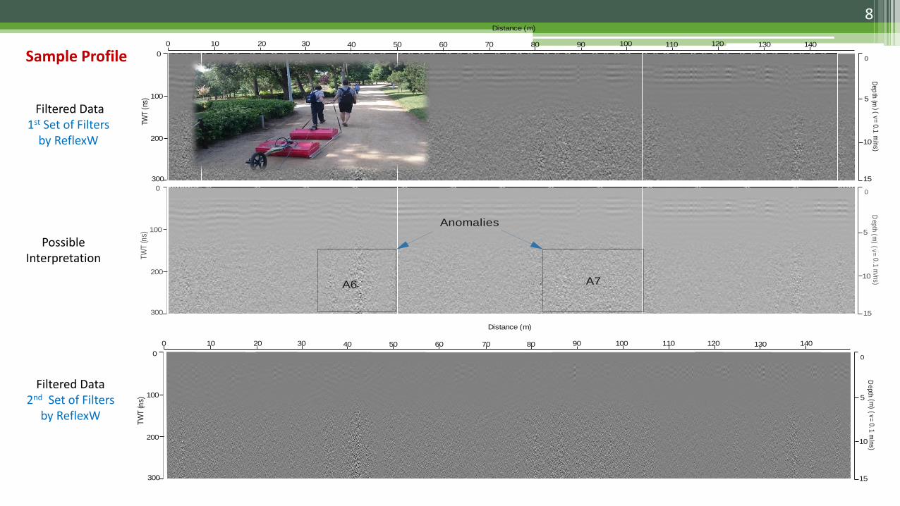
Sample Profile

10

15

5

De

pth

(m) ( v

= 0

.1 m

/ns

)Distance ( )m

300

200

100

TWT

(ns

)

0 0

130 140110 1201009080706050403020100

10

15

5

De

pth

(m) ( v

= 0

.1 m

/ns

)

300

200

100

TW

T (n

s)

0 0

A6 A7

Anomalies

10

15

5

De

pth

(m) ( v

= 0

.1 m

/ns

)

Distance ( )m

300

200

100

TW

T (n

s)

0 0

130 140110 1201009080706050403020100

Filtered Data1st Set of Filters

by ReflexW

Possible Interpretation

Filtered Data2nd Set of Filters

by ReflexW

9

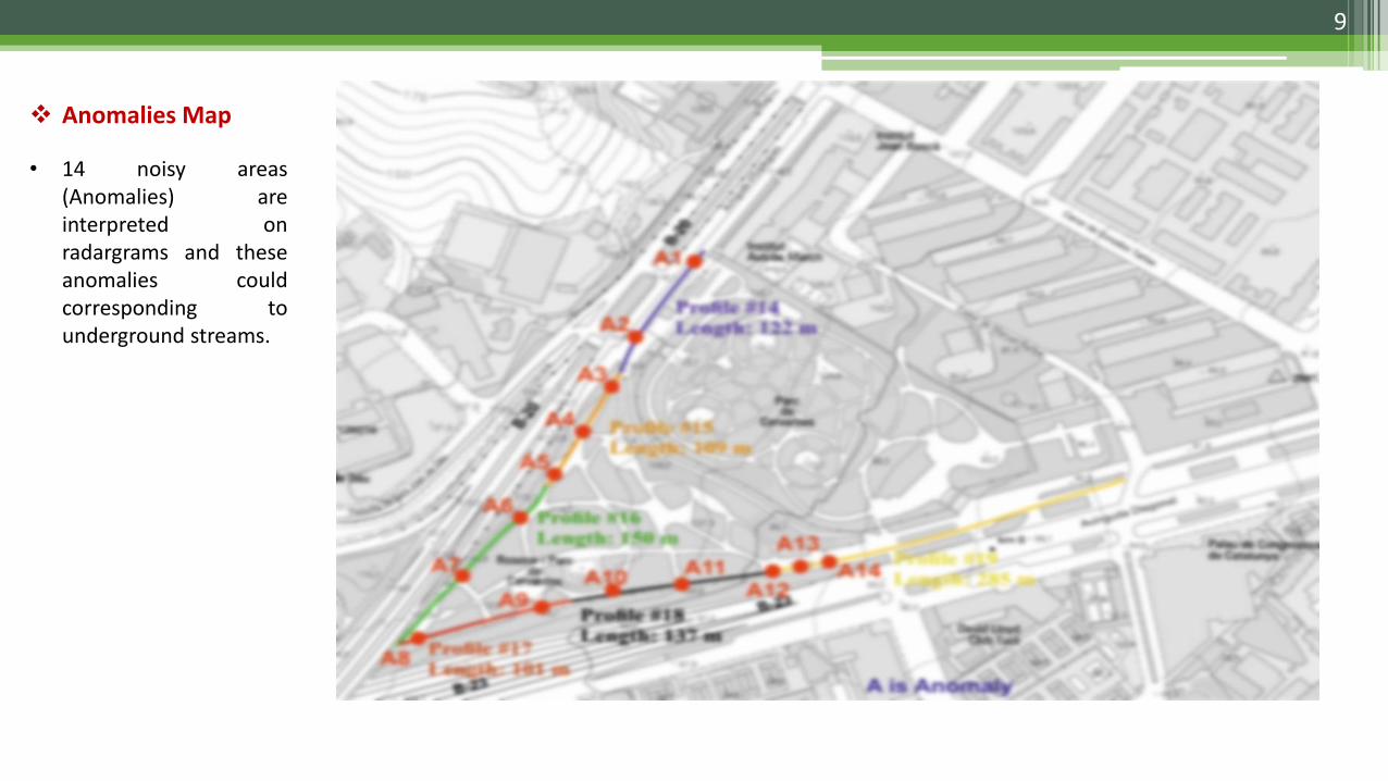
❖ Anomalies Map

• 14 noisy areas(Anomalies) areinterpreted onradargrams and theseanomalies couldcorresponding tounderground streams.

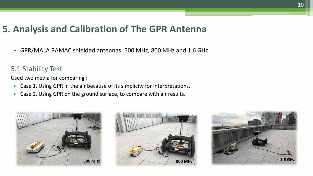
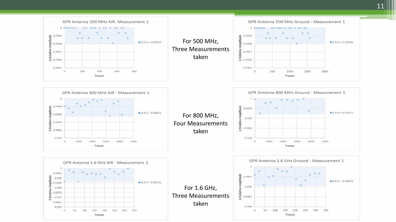
5. Analysis and Calibration of The GPR Antenna

• GPR/MALA RAMAC shielded antennas: 500 MHz, 800 MHz and 1.6 GHz.

5.1 Stability Test Used two media for comparing ;

• Case 1. Using GPR in the air because of its simplicity for interpretations.

• Case 2. Using GPR on the ground surface, to compare with air results.

10

500 MHz 800 MHz 1.6 GHz

11

For 500 MHz, Three Measurements

taken

For 800 MHz, Four Measurements

taken

For 1.6 GHz, Three Measurements

taken

12

GPR Antenna GPR

Measurements

1st Case 2nd Case

AIR GROUND

Δ A Δ A

500 MHz 1 0.00019 0.00006

2 0.00013 0.00016

3 0.00019 0.00009

AVERAGE 0.00017 0.00010

800 MHz 1 0.00041 0.00075

2 0.00081 0.00125

3 0.00109 0.00041

4 0.00050 0.00025

AVERAGE 0.00070 0.00066

1.6 GHz 1 0.00131 0.00092

2 0.00417 0.00188

3 0.00246 0.00665

AVERAGE 0.00265 0.00315

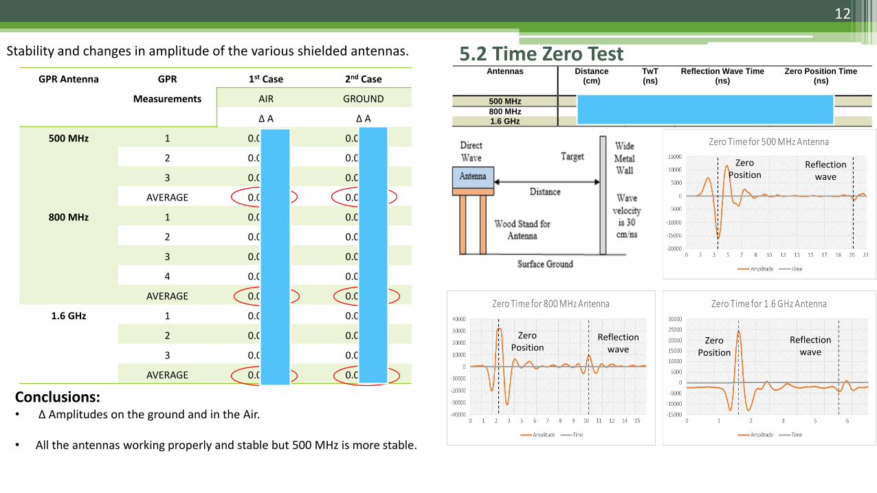
Stability and changes in amplitude of the various shielded antennas. 5.2 Time Zero Test Antennas Distance

(cm)

TwT (ns)

Reflection Wave Time (ns)

Zero Position Time (ns)

500 MHz 240 16 20 4

800 MHz 120 8 10 2 1.6 GHz 60 4 5.5 1.5

Zero Position

Reflectionwave

Zero Position

Zero Position

Reflectionwave

Reflectionwave

Conclusions:• Δ Amplitudes on the ground and in the Air.

• All the antennas working properly and stable but 500 MHz is more stable.

13

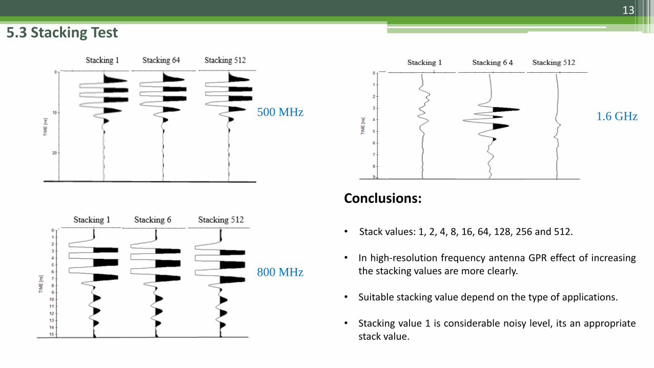
5.3 Stacking Test

500 MHz

800 MHz

1.6 GHz

Conclusions:

• Stack values: 1, 2, 4, 8, 16, 64, 128, 256 and 512.

• In high-resolution frequency antenna GPR effect of increasingthe stacking values are more clearly.

• Suitable stacking value depend on the type of applications.

• Stacking value 1 is considerable noisy level, its an appropriatestack value.

4

14

[1] Joachim Ender. 98 Years of the RADAR Principle: The Inventor Christian Hülsmeyer. EUSAR 2002

[2] Kozlovsky, E.A. (ed), 1989. Encyclopaedia of Mining (in Russian). Ed. Sovietic Encyclopaedia. 4, 285-286.

[3] Finkelshtein, M.I., Kutev, V.A., Zolotared, V.P., 1986. Applications of ground penetrating radar in geological engineering (inRussian). Ed. Nedra. Moscow.

[4] http://www.radarworld.org/huelsmeyer.html.

[5]http://www.ieeeghn.org/wiki/index.php/Radar_during_World_War_II#Radar_during_World_War_II (access: 2014/05/26).

[6] HULSENBECK et al.: German Pat. No. 489434, 1926

[7] STEENSON, B. 0.: 'Radar methods for the exploration of glaciers'. PhD Thesis, Calif. Inst. Tech., Pasadena, CA, USA, 1951

References

Many Thanks for your attention

15