GPGPU Performance and Power EstimationUsing Machine Learning

Gene Wu∗, Joseph L. Greathouse†, Alexander Lyashevsky†, Nuwan Jayasena†, Derek Chiou∗

∗Electrical and Computer EngineeringThe University of Texas at Austin{Gene.Wu, Derek}@utexas.edu

†AMD ResearchAdvanced Micro Devices, Inc.

{Joseph.Greathouse, Alexander.Lyashevsky, Nuwan.Jayasena}@amd.com

Abstract—Graphics Processing Units (GPUs) have numer-ous configuration and design options, including core frequency,number of parallel compute units (CUs), and available memorybandwidth. At many stages of the design process, it is importantto estimate how application performance and power are impactedby these options.

This paper describes a GPU performance and power esti-mation model that uses machine learning techniques on mea-surements from real GPU hardware. The model is trained ona collection of applications that are run at numerous differenthardware configurations. From the measured performance andpower data, the model learns how applications scale as the GPU’sconfiguration is changed. Hardware performance counter valuesare then gathered when running a new application on a singleGPU configuration. These dynamic counter values are fed intoa neural network that predicts which scaling curve from thetraining data best represents this kernel. This scaling curve isthen used to estimate the performance and power of the newapplication at different GPU configurations.

Over an 8× range of the number of CUs, a 3.3× range ofcore frequencies, and a 2.9× range of memory bandwidth, ourmodel’s performance and power estimates are accurate to within15% and 10% of real hardware, respectively. This is comparableto the accuracy of cycle-level simulators. However, after an initialtraining phase, our model runs as fast as, or faster than theprogram running natively on real hardware.

I. INTRODUCTION

Graphics processing units (GPUs) have become standarddevices in systems ranging from cellular phones to supercom-puters. Their designs span a wide range of configurations andcapabilities, from small, power-efficient designs in embeddedsystems on chip (SoCs) to large, fast devices meant to prioritizeperformance. Adding to the complexity, modern processorsreconfigure themselves at runtime in order to maximize per-formance under tight power constraints. These designs willrapidly change core frequency and voltage [1], [43], modifyavailable bandwidth [14], and quickly power gate unusedhardware to reduce static power usage [31], [37].

With this wide range of possible configurations, it is criticalto rapidly analyze application performance and power. Earlyin the design process, architects must verify that their plan willmeet performance and power goals on important applications.Software designers, similarly, would like to verify performancetargets on a wide range of devices. These estimates can evenresult in better dynamic reconfiguration decisions [46], [49].

Design-time estimates are traditionally performed usinglow-level simulators such as GPGPU-Sim [8], which can becarefully configured to yield accurate estimates, often within

10-20% of real hardware. The performance of such simulators,however, precludes their use for online analysis or large designspace explorations. GPGPU-Sim, for instance, runs millionsof times slower than native execution [35]. Such overheadsoften result in the use of reduced input sets, which can furtherdecrease accuracy, or sampling techniques which can still runmany times slower than real hardware if they model eachsample in a slow simulator [52].

To alleviate this problem, researchers have built a varietyof analytic performance and power models [6], [23], [28], [30],[32], [38], [40], [45], [54], [55]. These range from estimatesthat use static code analyses [6] to linear regressions basedon hardware performance counters [28]. These models areprimarily built for, and trained on, single GPU configurations.This can yield accurate estimates but limits their ability tomodel large design spaces or runtime hardware changes.

This paper focuses on rapidly estimating the performanceand power of GPUs across a range of hardware configurations.We begin by measuring a collection of OpenCLTM kernels ona real GPU at various core frequencies, memory bandwidths,and compute unit (CU) counts. This allows us to build a set ofscaling surfaces that describe how the power and performanceof these applications change across hardware configurations.We also gather performance counters, which give a fingerprintthat describes each kernel’s use of the underlying hardware.

Later, when analyzing previously unseen kernels, we gatherthe execution time, power, and performance counters at asingle hardware configuration. Using machine learning (ML)methods, we use these performance counter values to predictwhich training kernel is most like this new kernel. We thenestimate that the scaling surface for that training kernel alsorepresents the kernel under test. This allows us to quicklyestimate the power and performance of the new kernel atnumerous other hardware configurations.

For the variables we can explore during the training phase,we find our ML-based estimation model to be as accurate asvalues commonly reported for microarchitectural simulations.We are able to estimate the performance of our test kernelsacross a 3.3× change in core frequency, a 2.9× changein memory bandwidth, and an 8× change in CUs with anaverage error of 15%. We are able to estimate dynamic powerusage across the same range with an average error of 10%.In addition, this is faster than low-level simulators; after anoffline training phase, online predictions across the range ofsupported settings takes only a single run on the real hardware.Subsequent predictions only require running the ML predictor,which can be much faster than running the kernel itself.

This work makes the following contributions:

• We demonstrate on real hardware that the performanceand power of General-purpose GPU (GPGPU) kernelsscale in a limited number of ways as hardware con-figuration parameters are changed. Many kernels scalesimilarly to others, and the number of unique scalingpatterns is limited.

• We show that, by taking advantage of the first insight,we can perform clustering and use machine learn-ing techniques to match new kernels to previouslyobserved kernels whose performance and power willscale in similar ways.

• We then describe a power and performance estimationmodel that uses performance counters gathered duringone run of a kernel at a single configuration to predictperformance and power across other configurationswith an average error of only 15% and 10%, respec-tively, at near-native-execution speed.

The remainder of this paper is arranged as follows. SectionII motivates this work and demonstrates how GPGPU kernelsscale across hardware configurations. Section III details ourML model and how it is used to make predictions. SectionIV describes the experimental setup we used to validate ourmodel and Section V details the results of these experiments.Section VI lists related work, and we conclude in Section VII.

II. MOTIVATION

This section describes a series of examples that motivatethe use high-level performance and power models beforeintroducing our own model based on ML techniques.

A. Design Space Exploration

Contemporary GPUs occupy a wide range of design pointsin order to meet market demands. They may use similarunderlying components (such as the CUs), but the SoCs mayhave dissimilar configurations. As an example, Table I listsa selection of devices that use graphics hardware based onAMD’s Graphics Core Next microarchitecture. As the datashows, the configurations vary wildly. At the extremes, theAMD RadeonTM R9 290X GPU, which is optimized formaximum performance, has 22× more CUs running at 2.9×the frequency and with 29× more memory bandwidth than thetablet-optimized AMD E1-6010 processor.

Tremendous effort goes into finding the right configurationfor a chip before expending the cost to design it. The perfor-mance of a product must be carefully weighed against factorssuch as area, power, design cost, and target price. Applicationsof interest are studied on numerous designs to ensure that aproduct will meet business goals.

Low-level simulators, such as GPGPU-Sim [8] allow ac-curate estimates, but they are not ideal for early design spaceexplorations. These simulators run 4-6 orders of magnitudeslower than native execution, which limits the applications(and inputs) that can be studied. In addition, configuringsuch simulators to accurately represent real hardware is time-consuming and error-prone [21], which limits the number ofdesign points that can be easily explored.

TABLE I: Products built from similar underlying AMD logicblocks that contain GPUs with very different configurations.

Max. Max.Name CUs Freq. DRAM BW

(MHz) (GB/s)AMD E1-6010 APU [22] 2 350 11

AMD A10-7850K APU [2] 8 720 35Microsoft Xbox OneTM processor [5] 12 853 68

Sony PlayStationr 4 processor [5] 18 800 176AMD RadeonTM R9-280X GPU [3] 32 1000 288AMD RadeonTM R9-290X GPU [3] 44 1000 352

One common way of mitigating simulation overheads isto use reduced input sets [4]. The loss of accuracy caused bythis method led to the development of more rigorous samplingmethods such as SimPoints [44] and SMARTS [51]. Thesecan reduce simulation time by two orders of magnitude whileadding errors of only 10-20% [52]. Nonetheless, this still runshundreds to thousands of times slower than real hardware.

High-level models are a better method of pruning thedesign space during early explorations. These models maybe less accurate than low-level simulators, but they allowrapid analysis of many full-sized applications on numerousconfigurations. We do not advocate for eliminating low-levelsimulation, as it offers valuable insight that high-level modelscannot produce. However, high-level models allow designers toprune the search space and only spend time building low-levelmodels for potentially interesting configurations.

B. Software Analysis

GPGPU software is often carefully optimized for thehardware on which it will run. With dozens of models onthe market at any point in time (as partially demonstratedin Table I), it is difficult to test software in every hardwareconfiguration that consumers will use. This can complicate thetask of setting minimum requirements, validating performancegoals, and finding performance and power regressions.

Low-level simulators are inadequate for this task, as theyare slow and require great expertise to configure and use. Inaddition, GPU vendors are loath to reveal accurate low-levelsimulators, as they can reveal proprietary design information.

High-level models are better for this task. Many existinghigh-level models focus on finding hardware-related bottle-necks, but they are limited to studying a single device configu-ration [23], [28], [32], [38], [55]. There are others that estimatehow an application would perform as parameters such asfrequency change [39]. We will later detail why these relativelysimple models have difficulty accurately modeling complexmodern GPUs. Nonetheless, their general goal matches ourown: provide fast feedback about application scaling.

C. Online Reconfiguration

Modern processors must optimize performance under tightpower budgets. Towards this end, dynamic voltage and fre-quency scaling (DVFS) varies core and memory frequency inresponse to demand [14], [31]. Recent publications also advo-cate for disabling GPU CUs when parallelism is least helpful[41]. We refer to these methods as online reconfiguration.

91

149

206

264

012

3

4

5

6

7

8

4 8 12 16 20 24 28 32

Normalized

 Perform

ance

120

178

235

(a) A compute-bound kernel.

91

149

206

264

00.5

1

1.5

2

2.5

3

3.5

4

4 8 12 16 20 24 28 32

Normalized

 Perform

ance

120

178

235

(b) A bandwidth-bound kernel.

91

149

206

264

0

1

2

3

4

5

6

7

4 8 12 16 20 24 28 32

Normalized

 Perform

ance

120

178

235

(c) A balanced kernel.

91

149

206

264

0

1

2

3

4

5

4 8 12 16 20 24 28 32

Normalized

 Perform

ance

120

178

235

(d) An irregular kernel.

Fig. 1: Four different GPGPU performance scaling surfaces. Frequency is held at 1 GHz while CUs and bandwidth are varied.

Advanced reconfiguration systems try to predict the effectof their changes on the total performance of the system. Forinstance, boosting a CPU’s frequency may prevent a nearbyGPU from reaching its optimal operating point, requiring on-line thermal models to maximize chip-wide performance [42].Similarly, using power and performance estimates to proac-tively choose the best voltage and frequency state (rather thanreacting only to the results of previous decisions) can enablepower capping solutions, optimize energy usage, and yieldhigher performance in “dark silicon” situations [46], [49].

Estimating how applications scale across hardware config-urations is a crucial aspect of these systems. These estimatesmust be made rapidly, precluding low-level simulators, andmust react to dynamic program changes, which limits the useof analytic models based on static analyses. We therefore studymodels that quickly estimate power and performance usingeasy-to-obtain dynamic hardware event counters.

D. High-Level GPGPU Model

The recurring theme in these examples is a desire for afast, relatively accurate estimation of performance and powerat different hardware configurations. Previous studies havedescribed high-level models that can predict performance atdifferent frequencies, which can be used for online optimiza-tions [24], [39], [45]. Unfortunately, these systems are limitedby their models designed after abstractions of real hardware.

Fig. 1 shows the performance of four OpenCLTM kernels ona real GPU. The performance (Y-axis) changes as the numberof active CUs (X-axis) and the available memory bandwidth(Z-axis) are varied. Frequency is fixed at 1 GHz.

Existing models that compare compute and memory workcan easily predict the applications shown in Fig. 1(a) and 1(b)because they are compute and bandwidth-bound, respectively.Fig. 1(c) is more complex; its limiting factor depends on ratioof CUs to bandwidth. This requires a model that handleshardware component interactions [23], [54].

Fig. 1(d) shows a performance effect that can be difficultto predict with simple models. Adding more CUs helps per-formance until a point, whereupon performance drops as moreare added. This is difficult to model using linear regression orsimple compute-versus-bandwidth formulae.

As more CUs are added, more pressure is put on the sharedL2 cache. Eventually, the threads’ working sets overflow theL2 cache, degrading performance. This effect has been shown

in simulation, but simple analytic models do not take it intoaccount [29], [34]. Numerous other non-obvious scaling resultsexist, but we do not detail them due to space constraints.Suffice to say, simple models have difficulty with kernels thatare constrained by complex microarchitectural limitations.

Nevertheless, our goal is to create a high-level modelthat we can use to estimate performance and power acrossa wide range of hardware configurations. As such, we buildan ML model that can perform these predictions quickly andaccurately.

We begin by training on a large number of OpenCL kernels.We run each kernel at numerous hardware configurations whilemonitoring power, performance, and hardware performancecounters. This allows us to collect data such as that shownin Fig. 1. We find that the performance and power of manyGPU kernels scale similarly. We therefore cluster similarkernels together and use the performance counter informationto fingerprint that scaling surface.

To make predictions for new kernels, we measure theperformance counters obtained from running that kernel at onehardware configuration. We then use them to predict whichscaling surface best describes this kernel. With this, we canquickly estimate the performance or power of a kernel at manyconfigurations. The following section details this process.

III. METHODOLOGY

We describe our modeling methodology in two passes.First, Section III-A describes the methodology at a high level,providing a conceptual view of how each part fits together.Then Section III-B, Section III-C, and Section III-D go intothe implementation details of the different parts of the model.For simplicity, these sections describe a performance model,but this approach can be applied to generate power models aswell.

A. Overview

While our methodology is amenable to modeling anyparameter that can be varied, for the purposes of this study, wedefine a GPU’s hardware configuration as its number of CUs,engine frequency, and memory frequency. We take as an inputto our predictor measurements gathered on one specific GPUhardware configuration called the base hardware configura-tion. Once a kernel has been executed on the base hardwareconfiguration, the model can be used to predict the kernel’sperformance on a range of target hardware configurations.

Training Set

Model Construction

Flow

GPU Hardware

Kernel

Model

Execution Time/power

Performance Counters

Target Hardware

Configuration

Target Execution Time/Power

Fig. 2: The model construction and usage flow. Trainingis done on many configurations, while predictions requiremeasurements from only one.

Kernel name 4,300,375 … 32,1000,1375 Perf. Count 1. Perf. Count. 2 …

Kernel 1

…..

Kernel N

CU count,Engine freq., Mem. freq,

Execution Times/Power Performance Counter Values gathered on base hardware configuration

Fig. 3: The model’s training set, which contains the perfor-mance or power of each training kernel for a range of hardwareconfigurations.

The model construction and usage flow are depicted inFig. 2. The construction algorithm uses a training data setcontaining execution times and performance counter valuescollected from executing training kernels on real hardware. Thevalues in the training set are shown in Fig. 3. For each trainingkernel, execution times and performance counter values acrossa range of hardware configurations are stored in the trainingset. The performance counter values collected while executingeach training kernel on the base hardware configuration arealso stored.

Once the model is constructed, it can be used to predictthe performance of new kernels, from outside the training set,at any target hardware configuration within the range of thetraining data. To make a prediction, the kernel’s performancecounter values and base execution time must first be gatheredby executing it on the base hardware configuration. These arethen passed to the model, along with the desired target hard-ware configuration, which will output a predicted executiontime at that target configuration. The model is constructed onceoffline but used many times. It is not necessary to gather atraining set or rebuild the model for every prediction.

Model construction consists of two major phases. In thefirst phase, the training kernels are clustered to form groupsof kernels with similar performance scaling behaviors acrosshardware configurations. Each resulting cluster represents onescaling behavior found in the training set.

In the simple example shown in Fig. 4, there are six trainingkernels being mapped to three clusters. Training kernels 1and 5 are both bandwidth bound and are therefore mapped

Cluster 1 Cluster 3 Cluster 2

Kernel 1 Kernel 2 Kernel 3

Kernel 4 Kernel 5 Kernel 6

Fig. 4: Forming clusters of kernel scaling behaviors. Kernelsthat scale in similar ways are clustered together.

Cluster 3

Cluster 2

Classifier

Cluster 1

Performance Counter Values (from base configuration)

? ? ?

Fig. 5: Building a classifier to map from performance countervalues to clusters.

to the same cluster. Kernel 3 is the only one of the six thatis purely compute bound, and it is mapped to its own cluster.The remaining kernels scale with both compute and memorybandwidth, and they are all mapped to the remaining cluster.While this simple example demonstrates the general approach,the actual model identifies larger numbers of clusters withmore complex scaling behaviors in a 4D space.

In the second phase, a classifier is constructed to predictwhich cluster’s scaling behavior best describes a new kernelbased on its performance counter values. The classifier, shownFig. 5, would be used to select between the clusters inFig. 4. The classifier and clusters together allow the modelto predict the scaling behavior of a new kernel across a widerange of hardware configurations using information taken fromexecuting it on the base hardware configuration. When themodel is asked to predict the performance of a new kernel ata target hardware configuration, the classifier is accessed first.The classifier chooses one cluster, and that cluster’s scalingbehavior is used to scale the baseline execution time to thetarget configuration in order to make the desired prediction.

Fig. 6 gives a detailed view of the model architecture.Notice that the model contains multiple sets of clusters andclassifiers. Each cluster set and classifier pair is responsiblefor providing scaling behaviors for a subset of the CU,engine frequency, and memory frequency parameter space. Forexample, the top cluster set in Fig. 6 provides informationabout the scaling behavior when CU count is 8. This set pro-vides performance scaling behavior when engine and memoryfrequencies are varied and CU count is fixed at 8. The exact

Cluster 1

Cluster 2

Cluster N

…

Cluster 1

Cluster 2

Cluster N

…

Cluster 1

Cluster 2

Cluster N

…

… …… …

CUs = 8set

CUs = 32set

Variable CU set

…

Classifier

Classifier

Classifier

Performance Counter Values(from base configuration)

475

925

1375

0

1

2

3

4

30

0

40

0

50

0

60

0

70

0

80

0

90

0

10

00

Memory FrequencyN

orm

aliz

ed P

erfo

rman

ce

Engine Frequency

475

925

1375

0

1

2

3

4

30

0

40

0

50

0

60

0

70

0

80

0

90

0

10

00

Memory Frequency

No

rma

lized

Per

form

an

ce

Engine Frequency

0

1

2

3

4

5

6

4 8 12 16 20 24 28 32

No

rma

lize

d

Pe

rfo

rman

ce

CU count

Base Config. Exec. Time & Target Config.

Target Config. Exec. Time

Fig. 6: Detailed architecture of our performance and power predictor. Performance counters from one execution of the applicationare used to find which cluster best represents how this kernel will scale as the hardware configuration is changed. Each clustercontains a scaling surface that describes how this kernel will scale when some hardware parameters are varied.

number of sets and classifier pairs in a model depends on thehardware configurations that appear in the training set.

The scaling information from these cluster sets allows scal-ing from the base to any other target configuration. By dividingthe parameter space into multiple regions and clustering thekernels once for each region, the model is given additionalflexibility. Two kernels may have similar scaling behaviors inone region of the hardware configuration space, but differentscaling in another region. For example, two kernels may scaleidentically with respect to engine frequency, but one may notscale at all with CU count while the other scales linearly.For cases like this, the kernels may be clustered together inone cluster set but not necessarily in others. Breaking theparameter space into multiple regions and clustering eachregion independently allows kernels to be grouped into clusterswithout requiring that they scale similarly across the entireparameter space. In addition, by building a classifier for eachregion of the hardware configuration space, each classifier onlyneeds to learn performance counter trends relevant to its region,which reduces their complexity.

The remainder of this section provides descriptions ofthe steps required to construct this model. The calculationof scaling values, which are used to describe a kernel’sscaling behavior, is described in Section III-B. Section III-Cdescribes how these are used to form sets of clusters. Finally,Section III-D describes the construction of the neural networkclassifiers.

B. Scaling Surfaces

Our first step is to convert the training kernel executiontimes into performance scaling values, which capture howthe kernels’ performance changes as the number of CUs,engine frequency, and memory frequency are varied. Scalingvalues are calculated for each training kernel and then putinto the clustering algorithm. Because we want to form groupsof kernels with similar scaling behaviors, even if they havevastly different execution times, the kernels are clustered usingscaling values rather than raw execution times.

To calculate scaling values, the training set executiontimes are grouped by kernel. Then, for each training kernel,a 3D matrix of execution times is formed. Each dimensioncorresponds to one of the hardware configuration parameters.In other words, the position of each execution time in thematrix is defined by the number of CUs, engine frequency,and memory frequency combination it corresponds to.

The matrix is then split into sub-matrices, each of whichrepresents one region of the parameter space. Splitting thematrix in this way will form the multiple cluster sets seenin Fig. 6. An execution time sub-matrix is formed for eachpossible CU count found in the training data. For example, iftraining set data have been gathered for CU counts of 8, 16,24, and 32, four sub-matrices will be formed per kernel.

The process to convert an execution time sub-matrix intoperformance scaling values is illustrated using the example inFig. 7. An execution time sub-matrix with a fixed CU countis shown in Fig. 7(a). Because the specific CU count does notchange any of the calculations, it has not been specified. Inthis example, it is assumed that the training set engine andmemory frequency both range from 400 MHz to 1000 MHzwith a step size of 200 MHz. However, the equations givenapply to any range of frequency values, and the reshaping ofthe example matrices to match the new range of frequencyvalues is straightforward.

Two types of scaling values are calculated from the ex-ecution times shown in Fig. 7. Memory frequency scalingvalues, shown in Fig. 7(b), capture how execution timeschange as memory frequency increases and engine frequencyremains the same. Engine frequency scaling values, shownin Fig. 7(c), capture how execution times change as enginefrequency increases and memory frequency remains the same.In the memory scaling matrix, each entry’s column positioncorresponds to a change in memory frequency and its rowposition corresponds to a fixed engine frequency. In the enginescaling matrix, each entry’s column position corresponds to achange in engine frequency and its row position correspondsto a fixed memory frequency.

t3,0

t2,0

t1,0

t0,0

t3,1

t2,1

t1,1

t0,1

t3,2

t2,2

t1,2

t0,2

t3,3

t2,3

t1,3

t0,3

1000

800

600

400

Mem. Freq. (MHz)

Engi

ne

Freq

. (M

Hz)

(a) Execution times

m3,0

m2,0

m1,0

m0,0

m3,1

m2,1

m1,1

m0,1

m3,2

m2,2

m1,2

m0,2

1000

800

600

400

Mem. Freq. (MHz)

Engi

ne

Freq

. (M

Hz)

𝑚𝑖,𝑗 =𝑡𝑖,𝑗+1

𝑡𝑖,𝑗

(b) Memory frequency scaling values.

e2,0

e1,0

e0,0

e2,1

e1,1

e0,1

e2,2

e1,2

e0,2

e2,3

e1,3

e0,3

800 to 1000

600 to 800

400 to 600

Mem. Freq. (MHz)

Engi

ne

Freq

. (M

Hz)

𝑒𝑖,𝑗 =𝑡𝑖+1,𝑗

𝑡𝑖,𝑗

(c) Engine frequency scaling values.

Fig. 7: Calculation of frequency scaling values.

As long as the CU counts of the base and target configura-tions remain the same, one or more of the shown scaling valuescan be multiplied with a base configuration execution time topredict a target configuration execution time. We will showhow to calculate the scaling factors to account for variableCU counts shortly. The example in Equation 1 shows howthese scaling values are applied. The base configuration hasa 400 MHz engine clock and a 400 MHz memory clock.The base execution time is t0,0. We can predict the targetexecution time, t3,3, of a target configuration with a 1000MHz engine clock and a 1000 MHz memory clock usingEquation 1. Scaling values can also be used to scale fromhigher frequencies to lower frequencies by multiplying thebase execution time with the reciprocals of the scaling values.For example, because m0,0 can be used to scale from a 400MHz to 600 MHz memory frequency, 1

m0,0can be used to

scale from a 600 MHz to 400 MHz memory frequency. Scalingexecution times in this way may not seem useful when onlytraining data is considered, as the entire execution time matrixis known. However, after the model has been constructed, thesame approach can be used to predict execution times fornew kernels at configurations that have not been run on realhardware.

t3,3 = t0,0

2∏j=0

e0,j

2∏i=0

mi,2 (1)

In addition to the engine and memory frequency scalingvalues, a set of scaling values is calculated to account forvarying CU count. A sub-matrix, from which CU scalingvalues can be extracted, is constructed. All entries of thisnew sub-matrix correspond to the base configuration engineand memory frequency. However, each entry corresponds toone of the CU counts found in the training data. An exampleexecution time sub-matrix with variable CU count is shown inFig. 8(a). A set of CU scaling behavior values are calculatedusing the template shown in Fig. 8(b).

To predict a target configuration execution time, the CUscaling values are always applied before applying any engineor memory frequency scaling values. The difference betweenthe base and target configuration CU counts determines which,if any, CU scaling values are multiplied with the base executiontime. After applying CU scaling values to the base executiontime, the resulting scaled value is further scaled using the

t3 t2 t1 t0

32 24 16 8

Compute Units

(a) Execution times.

𝑐𝑖 =𝑡𝑖+1𝑡𝑖

c2 c1 c0

Compute Units

(b) Compute unit scaling values.

Fig. 8: Calculation of CU scaling values.

memory and engine frequency sets corresponding to the targetCU count. This yields a target execution time that correspondsto the CU count, engine frequency, and memory frequency ofthe target configuration.

C. Clustering

K-means clustering is used to create sets of scaling behav-iors representative of the training kernels. The training kernelsare clustered multiple times to form multiple sets of clusters.Each time, the kernels are clustered based on a different setof the scaling values discussed in Section III-B. Each set ofclusters is representative of the scaling behavior of one regionof the hardware configuration parameter space. The trainingkernels are clustered once for each CU count available inthe training set hardware configurations and once based ontheir scaling behavior as CU count is varied. For example, iftraining data is available for CU counts of 8, 16, 24, and 32,the training kernels will be clustered five times and producefive independent cluster sets. Four sets of clusters account forscaling behavior with varying engine and memory frequency,and one set accounts for varying CU count.

Before each clustering attempt, a feature vector is formedfor each training kernel. When forming clusters for a specificCU count, the appropriate engine and memory frequency scal-ing values (see Fig. 7) are chosen and concatenated togetherto form the feature vector. When forming the variable CUcount clusters, the training kernel CU scaling values (seeFig. 8) are chosen. After each training kernel has a featurevector, the training kernels are clustered based on the valuesin these feature vectors using K-means clustering. The K-means algorithm will cluster the kernels with similar scalingbehaviors together. For example, purely memory bound kernelswill be clustered together and purely compute bound kernels

TABLE II: Classifier feature list.

VALUInsts % instructions that are vector ALU instructionsSALUInsts % instructions that are scalar ALU instructionsVFetchInsts % instructions that are vector fetch instructionsSFetchInsts % instructions that are scalar fetch instructionsVWriteInsts % instructions that are vector write instructionsLDSInsts % instructions that are local data store insts.VALUUtilization % active vector ALU threads in the average waveVALUBusy % of time vector instructions are being processedSALUBusy % of time scalar instructions are being processedCacheHit % L2 cache access that hitMemUnitBusy % time the average CU’s memory unit is activeMemUnitStalled % time the memory unit is waiting for dataWriteUnitStalled % time the average write unit is stalledLDSBankConflict % time stalled on LDS bank conflictsOccupancy % of maximum number of wavefronts that

can be scheduled in any CU (Static per kernel)V IPC Vector instruction throughputMemTime Ratio of estimated time processing memory

requests to total timeFetchPerLoadByte Average number of load instructions per

byte loaded from memoryWritePerStoreByte Average number of store instructions per

byte stored from memoryNumWorkGroups Number of work groups (Saturates at 320)ReadBandwidth Average read bandwidth usedWriteBandwidth Average write bandwidth used

will be clustered together. It is possible for some kernels to begrouped into the same cluster in one set of clusters, but notin another set of clusters. This can happen for many reasons.For example, kernels may scale similar with engine frequency,but differently with CU count. Kernels scaling similarly withengine or memory frequency at low CU counts, but differentlyat high CU counts can also cause this behavior. Clusteringmultiple times with different sets of scaling values, rather thanusing one set of clusters using all scaling values at once, allowsthese kinds of behaviors to be taken into account.

Each cluster’s centroid (i.e., the vector of mean scalingvalues calculated from kernels belonging to the cluster) is usedas its representative set of scaling values. Centroids take thesame form as the scaling value matrices shown in either Fig. 7or Fig. 8, depending on which type of scaling values they wereformed from. When a cluster is chosen by a classifier in thefinal model, its centroid scaling values are applied to scale abase configuration execution time as described in Section III-B.

The number of clusters is a parameter of the K-meansclustering algorithm. Using too few clusters runs the risk ofunnecessarily forcing kernels with different scaling behaviorsinto the same cluster. The resulting centroid will not berepresentative of any particular kernel. On the other hand,using too many clusters runs the risk of overfitting the trainingset. In addition, the complexity of the classifier increases as thenumber of clusters increases. Training the classifier becomesmore difficult when too many clusters are used.

D. Classifier

After forming representative clusters, the next step is tobuild classifiers, which are implemented using neural networks,that can map kernels to clusters using performance countervalues. One neural network is built and trained per cluster set.The features used as inputs to the neural networks are listedin Table II. We use AMD CodeXL to gather a collection of

performance counters for each kernel, and all of our featuresare either taken directly from these or derived from them. Be-fore training the neural networks, the minimum and maximumvalues of each feature in Table II are extracted from the trainingset. Using its corresponding minimum and maximum values,each training set feature value is normalized to fall between 0and 1. The normalized feature values are then used to train theneural network. This avoids the complications of training theneural network using features with vastly different orders ofmagnitude. All training set minimum and maximum featuresare stored away so that the same normalization process can beapplied each time the model is used.

The neural network topology is shown in Fig. 9. The neuralnetwork outputs one value, between 0 and 1, per cluster inits cluster set. The cluster with the highest output value isselected as the chosen cluster for the kernel. We build a threelayer, fully connected neural network. The input layer is linearand the hidden and output layers use sigmoid functions. Thetopology of the network can be seen in Fig. 9. The numberof input nodes is determined by the number of performancecounters and the number of output nodes is determined by thenumber of clusters. We set the number of hidden layer nodesto be equal to the number of output nodes.

After construction, the neural network is used to selectwhich clusters best describe the scaling behavior of the kernelthat the user wishes to study. The neural networks use thekernel’s normalized feature values, measured on the base hard-ware configuration, to choose one cluster from each cluster set.The centroids of the selected clusters are used as the kernel’sscaling values. The predicted target configuration executiontime is then calculated by multiplying the base hardwareconfiguration execution time by the appropriate scaling values,as described in Section III-B.

…

…

…

Perf. Counter 0

Perf. Counter 1

Perf. Counter N

Cluster 0

Cluster 1

Cluster M

Fig. 9: Neural network topology.

IV. EXPERIMENTAL SETUP

In order to validate the accuracy of our performanceand power prediction models, we execute a collection ofOpenCLTM applications on a real GPU while varying its hard-ware configuration. This allows us to measure the power andperformance changes between these different configurations.

We used an AMD RadeonTM HD 7970 GPU as our testplatform. By default, this GPU has 32 compute units (2048 ex-ecution units), which can run at up to 1 GHz, and 12 channelsof GDDR5 memory running at 1375 MHz (yielding 264 GB/sof DRAM bandwidth). All of our experiments were performedon a CentOS 6.5 machine running the AMD CatalystTM graph-ics drivers version 14.2 beta 1.3. We used the AMD APP SDK

v2.9 as our OpenCL implementation and AMD CodeXL v1.3to gather the GPU performance counters for each kernel.

As this work is about predicting performance and powerat various hardware configurations, we modified the firmwareon our GPU to support changes to the number of activeCUs and both the core and memory frequencies. All of ourbenchmarks are run at 448 different hardware configurations:a range of eight CU settings (4, 8, . . . , 32), eight corefrequencies (300, 400, . . . , 1000 MHz), and seven memoryfrequencies (475, 625, . . . , 1375 MHz). For each kernel inevery benchmark at all of these configurations, we gather theOpenCL kernel execution time, performance counters fromAMD CodeXL, and the average estimated power of that kernelover its execution.

The AMD Radeon HD 7970 GPU estimates the chip-wide dynamic power usage by monitoring switching eventsthroughout the core. It accumulates these events and updatesthe power estimates every millisecond [19]. We read thesevalues using the system’s CPU. We use these dynamic powervalues as the basis for our power model because static powerdoes not directly depend on the kernel’s execution.

We run GPGPU benchmarks from a number of suites: 13from Rodinia v2.41 [9], eight from SHOC2 [13], three fromOpenDwarfs3 [18], seven from Parboil4 [47], four from thePhoronix Test Suite5, eight from the AMD APP SDK samples6,and six custom applications modeled after HPC workloads7.Because the power readings from our GPU’s firmware areonly updated every millisecond, we only gather data fromkernels that either last longer than 1 ms on our fastest GPUconfiguration or which are idempotent and can be repeatedlyrun back-to-back. This yields 108 kernels across these 49applications, which we do not list due to space constraints.

The data from a random 80% of the 108 kernels were usedto train and construct our ML model, while the data from theremaining 20% were used for validation.

V. EXPERIMENTAL RESULTS

First, we evaluate the accuracy of our model for perfor-mance prediction. Section V-A provides a detailed analysis ofperformance model accuracy across different base hardwareconfigurations. Section V-B explores the model’s sensitivity tothe number of representative clusters used. Then, Section V-Cevaluates our approach for modeling power consumption.

A. Performance Model Accuracy

The base hardware configuration used is a key parameter ofthe model and can influence its accuracy. To study the relation-ship between model accuracy and base hardware configuration,a model was constructed for every one of the 448 possible base

1Rodinia: backprop, b+tree, cfd, gaussian, heartwall, hotspot, kmeans,lavaMD, leukocyte, lud, particlefilter, srad, streamcluster

2SHOC: DeviceMemory, MaxFlops, BFS, FFT, GEMM, Sort, Spmv w/additional CSR-Adaptive algorithm [20], Triad

3OpenDwarfs: crc, swat, gem4Parboil: stencil, mri-gridding, lbm, sad, histo, mri-q, cutcp5Phoronix: juliaGPU, mandelbulbGPU, smallptGPU, MandelGPU6AMD APP SDK: NBody, BlackScholes, BinomialOption, DCT, Eigen-

Value, FastWalshTransform, MersenneTwister, MonteCarloAsian7Custom: CoMD, LULESH, miniFE, XSBench, BPT [11], graph500 [12]

4 8 12 16 20 24 28 32 Legend

475 20.4  18.2  20.5  20.7  23.5  25.9  26.5  31.6  10.0     

625 20.3  15.5  14.4  13.5  16.7  21.1  20.2  21.2  15.0     

775 24.7  15.6  11.9  13.1  13.3  17.0  17.3  19.4  20.0     

925 14.5  13.7  11.3  13.5  14.2  12.9  13.4  17.2  25.0     

1075 13.5  13.7  13.0  12.6  13.5  13.6  13.2  18.3  30.0     

1225 15.8  16.3  12.2  10.6  9.0     13.5  11.8  14.2 

1375 15.5  11.1  12.8  10.8  11.1  11.6  12.7  11.5 

CU Count

Memory Frequency (MHz)

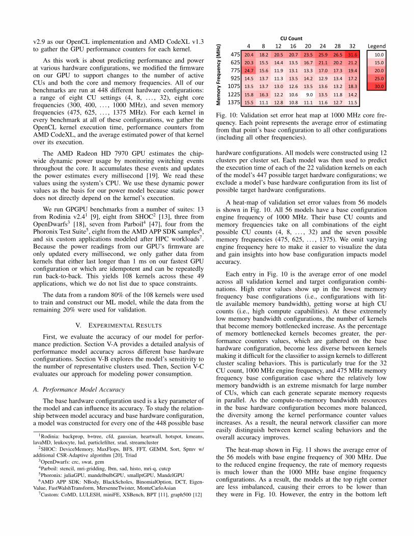
Fig. 10: Validation set error heat map at 1000 MHz core fre-quency. Each point represents the average error of estimatingfrom that point’s base configuration to all other configurations(including all other frequencies).

hardware configurations. All models were constructed using 12clusters per cluster set. Each model was then used to predictthe execution time of each of the 22 validation kernels on eachof the model’s 447 possible target hardware configurations; weexclude a model’s base hardware configuration from its list ofpossible target hardware configurations.

A heat-map of validation set error values from 56 modelsis shown in Fig. 10. All 56 models have a base configurationengine frequency of 1000 MHz. Their base CU counts andmemory frequencies take on all combinations of the eightpossible CU counts (4, 8, . . . , 32) and the seven possiblememory frequencies (475, 625, . . . , 1375). We omit varyingengine frequency here to make it easier to visualize the dataand gain insights into how base configuration impacts modelaccuracy.

Each entry in Fig. 10 is the average error of one modelacross all validation kernel and target configuration combi-nations. High error values show up in the lowest memoryfrequency base configurations (i.e., configurations with lit-tle available memory bandwidth), getting worse at high CUcounts (i.e., high compute capabilities). At these extremelylow memory bandwidth configurations, the number of kernelsthat become memory bottlenecked increase. As the percentageof memory bottlenecked kernels becomes greater, the per-formance counters values, which are gathered on the basehardware configuration, become less diverse between kernelsmaking it difficult for the classifier to assign kernels to differentcluster scaling behaviors. This is particularly true for the 32CU count, 1000 MHz engine frequency, and 475 MHz memoryfrequency base configuration case where the relatively lowmemory bandwidth is an extreme mismatch for large numberof CUs, which can each generate separate memory requestsin parallel. As the compute-to-memory bandwidth resourcesin the base hardware configuration becomes more balanced,the diversity among the kernel performance counter valuesincreases. As a result, the neural network classifier can moreeasily distinguish between kernel scaling behaviors and theoverall accuracy improves.

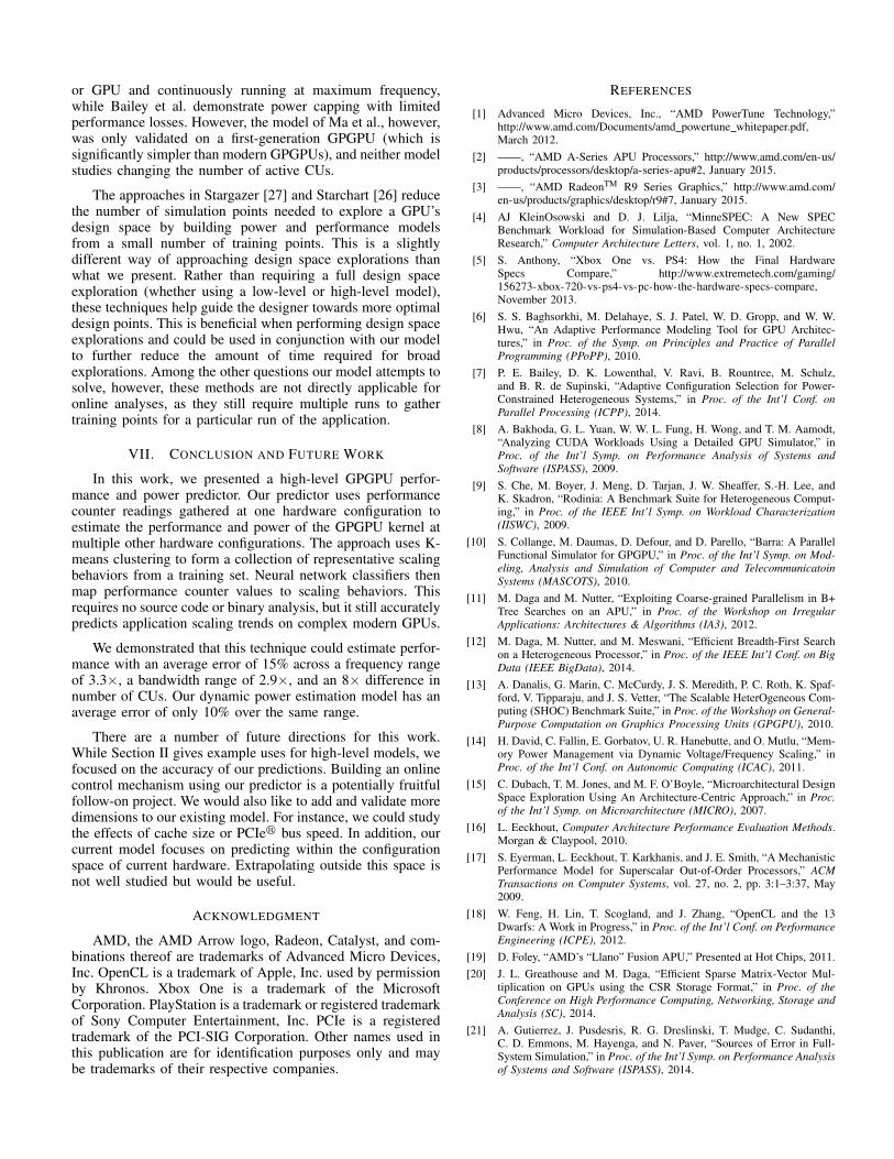
The heat-map shown in Fig. 11 shows the average error ofthe 56 models with base engine frequency of 300 MHz. Dueto the reduced engine frequency, the rate of memory requestsis much lower than the 1000 MHz base engine frequencyconfigurations. As a result, the models at the top right cornerare less imbalanced, causing their errors to be lower thanthey were in Fig. 10. However, the entry in the bottom left

4 8 12 16 20 24 28 32 Legend

475 21.7  16.3  10.6  11.4  12.1  11.4  13.7  15.1  10.0     

625 22.3  22.7  12.0  10.7  14.5  10.2  13.4  15.1  15.0     

775 15.9  20.9  15.8  13.5  12.0  15.8  16.7  14.3  20.0     

925 18.2  13.5  14.7  12.7  13.0  14.7  16.8  18.6  25.0     

1075 17.9  16.4  12.7  11.8  13.9  15.8  17.2  13.7  30.0     

1225 15.8  20.1  14.5  11.7  13.7  16.9  17.6  19.4 

1375 26.9  12.3  14.8  12.1  12.0  14.9  16.7  18.3 

CU CountMemory Frequency (MHz)

Fig. 11: Validation set error heat map at 300 MHz frequency.

corner of Fig. 11 is higher. This entry represents a model builtwith a base configuration of four CUs, a 300 MHz enginefrequency, and a 1375 MHz memory frequency, the highestmemory bandwidth to compute power configuration. In thisbase hardware configuration, only the most memory boundkernels will stress the memory system. This again results inless diversity in performance counter signatures similarly tothe previously discussed high error base configuration, butwith a large fraction of kernels limited entirely by computethroughput. This again means that the classifier will have aharder time distinguishing between kernel scaling behaviorsusing the base configuration’s performance counter values.

We generated heat-maps similar to Fig. 10 and Fig. 11using each of the remaining possible base hardware configu-ration engine frequencies. The results of these heat-maps aresummarized in Fig. 12. Each box and whisker set shows thedistribution of the average error of models with a common baseengine frequency. The lines through the middle of the boxesrepresent the distribution averages. The ends of the boxesrepresent the standard deviation of the distributions and theends of the whiskers represent the maximum and minimum ofthe errors. The best distribution is seen with a 500 MHz baseengine frequency, which supports the idea that configurationsin the middle of the design space make better base hardwareconfigurations. However, the distributions also show that evenfor more extreme base engine frequencies, it is still possibleto find a good base hardware configuration by choosing theappropriate base CU count and memory frequency to balanceout the configuration.

B. Sensitivity to the Number of Clusters

In this section, we discuss model accuracy as we vary thenumber of clusters per set. We built models using 2, 4, . . . , 20clusters per set and five different base hardware configurationsfor a total of 50 models. We then analyzed each model’serror for the 447 possible target hardware configurations (weexclude the base configuration from the targets). Section V-B1discusses model accuracy as cluster count is varied and Sec-tion V-B2 discusses how the major sources of modeling errorsshift with cluster count.

1) Overall Error: Fig. 13 shows the average error acrossthe validation kernel set as the number of clusters per clusterset varies for five base hardware configurations. The x-axisis labeled with the model base hardware configuration. Thelabels list the base CU count first, engine frequency second,and memory frequency third. The average error across the fivebase configurations is shown on the far right. Because the

0

5

10

15

20

25

30

35

300 400 500 600 700 800 900 1000

Erro

r %

Engine Frequency (MHz)

Fig. 12: Error vs. base hardware configuration.

010203040506070

Error %

Base Configuration

2 Clusters

4 Clusters

6 Clusters

8 Clusters

10 Clusters

12 Clusters

14 Clusters

16 Clusters

18 Clusters

20 Clusters

Fig. 13: Validation set error variation across cluster count.

cluster centroids and neural network weights are randomlyinitialized, the error values include some random variance.As shown earlier, the error is higher for models generatedfrom base hardware configurations with imbalanced computeto memory bandwidth ratios. In particular, using a 32 CU,1000 MHz engine frequency and 475 MHz memory frequencyconfiguration yields error values consistently higher acrossall cluster settings explored. However, the overall error trendacross the sampled base hardware configurations is similar.Model error trends downward until around 12 clusters. Forcluster counts greater than 12, error remains relatively constant.

Fig. 14 provides a more detailed breakdown of validationset error distribution as the number of clusters is varied. Thedistributions of two, six, and twelve cluster count models areshown as histograms. For each cluster count, we aggregatedthe error values across the five base configurations shownin Fig. 13. Because these models were evaluated using 22

0

5000

10000

15000

20000

25000

30000

Nu

mb

er

of

Dat

a p

oin

ts

Error

2 Clusters

6 Clusters

12 Clusters

Fig. 14: Validation set error distribution.

validation kernels and 447 target configurations, a total of49,170 (5×22×447) error values are represented for each ofthe three cluster counts. The first 10 bins of the histogramrepresent 10 percent error ranges (e.g., the first bin containsall data points with less than 10% error, the second bin containsall data points with greater than or equal to 10% error and lessthan 20% error, etc.). The final bin contains all data pointswith greater than or equal to 100% error. Going from low tohigh error bins, the number of model predictions falling ineach bin exhibits exponential decay (until the last bin, whichcorresponds to a greater range of values than the other bins).The number of data points in low error bins is higher and therate of decay is faster for models with more clusters.

2) Sources of Errors: There are two major sources of errorin the model. The first is poorly formed clusters. This can becaused by a poor training set, a typical concern encounteredwhen applying machine learning techniques that require atraining set. The number of clusters created by the clusteringalgorithm will also have a large impact on model accuracy.Using too few clusters will fail to capture the diverse rangeof scaling behaviors. Using too many clusters introduces thepossibility of over-fitting the model to the training set. Thesecond source of modeling error comes from the classificationstep. Even with a set of well-formed clusters, there will betimes the neural network classifier has difficulty classifying akernel to its appropriate cluster. Misclassifying a kernel willoften result in large performance prediction error.

To gain insight into how these two sources of error behave,we construct some models with an oracle classifier in placeof the neural network and compare them to our originalmodel described in Section III. The oracle models can onlybe applied to the training data set it was constructed with.For any kernel in the training data set, an oracle classifierchooses the exact cluster that the k-means cluster algorithmassigned it to, while the original, unmodified model uses theneural network classifier to pick an appropriate cluster basedoff performance counter values. When applying a model withan oracle classifier to its own training set, all error can beattributed to clustering. Comparing the oracle and unmodifiedmodels allows us to gain insight into the interaction betweenthe clustering and classification errors. Because the models areonly being applied to the training data set in this test, we canignore the possibilities of a non-representative training set andof over-fitting.

Both types are constructed using 2, 4, . . . , 20 clustersfor the five base hardware configurations shown in Fig. 13.We use the models to predict the execution times of eachkernel in the training data set for 447 different target hard-ware configurations and compare the oracle and unmodifiedmodel errors. The results are shown Fig. 15. We averagederror across base configurations, kernels, and target hardwareconfigurations to more clearly display accuracy vs. numberof clusters for unmodified, neural network models and oraclemodels. The oracle model error monotonically decreases asthe number of clusters increases and will decrease to zeroas the number of clusters approaches the number of trainingkernels. If each kernel has its own cluster, there will beno averaging of scaling surfaces within the clusters. Thismeans that any kernels scaling behavior in the training setcan be perfectly reproduced. The oracle classifier will never

0

5

10

15

20

25

30

2 4 6 8 10 12 14 16 18 20

Erro

r %

Clusters

Neural Network

Oracle

Fig. 15: Training set error variation with number of clusters.

0

2

4

6

8

10

12

14

Error %

Base Configuration

2 Clusters

4 Clusters

6 Clusters

8 Clusters

10 Clusters

12 Clusters

14 Clusters

16 Clusters

18 Clusters

20 Clusters

Fig. 16: Power model validation set error.

misclassify. However, the neural network classifier’s task be-comes more difficult as the number of clusters grows. Thisis demonstrated empirically in Fig. 15. Notice that the neuralnetwork classifier model error remains relatively unchanged ateight or more clusters despite the fact that the oracle modelerror continues to decrease. These results demonstrate thatwhile a greater number of clusters leads to more preciseclusters, it also complicates kernel classification. Eventuallythe potential accuracy gains offered by additional clusters isoffset by increased classification errors.

C. Power Model

In addition to performance modeling, we applied ourmethodology to create power models. We studied the powermodel accuracy versus the number of clusters using the sameexperimental set up used for the performance modeling exper-iments. We gathered the power values from hardware powermonitors in our GPU, which are deterministic estimates ofdynamic power based on switching activity in the cores. Assuch, we are training on and validating against a digital model,rather than analog measurements. This may make it easier topredict, as the values used will be less noisy.

Just like with the performance models, power models wereconstructed using 2, 4, . . . , 20 clusters for five base hardwareconfigurations. The power models’ errors on the validation setis presented in Fig. 16. As before, there is some randomnessin the results due to the randomized initial values of thecluster centroids and neural network weights. The errors ofthe models are fairly similar when more than two clusters areused. This suggests that the power behaviors are less diversethan the performance behaviors. The power model validationset errors, which are under 10% for most cluster configurations,

0

5000

10000

15000

20000

25000

30000

35000N

um

be

r o

f D

ata

po

ints

Error

2 Clusters

6 Clusters

12 Clusters

Fig. 17: Power model error distribution.

are also lower than the performance model validation errors.In addition, the variability of the error across base hardwareconfigurations is much smaller for power than it was forperformance modeling.

The power model validation error distribution is shown asa histogram in Fig. 17. Compared to the distribution of errorsin the performance model, the number of tests in the low errorbins is much higher. There is a large improvement from twoto six clusters and very little change from six to 12 clusters,which suggests that relatively few clusters are need to capturethe power scaling behaviors.

VI. RELATED WORK

Performance and power prediction are important topics,and Eeckhout gives an excellent overview of the literaturein this area [16]. The bulk of these works focus on CPUs,which were traditionally a system’s primary computation de-vice. Unfortunately, CPU-focused techniques are inadequatefor modeling GPUs. Mechanistic models are necessarily tiedto the CPU’s microarchitecture [17], [48], while more abstractmodels often rely on low-level data from the hardware orsimulator [15], [25], [33].

GPU performance and power estimation often uses low-level tools like GPGPU-Sim [8], Multi2Sim [50], andBarra [10] for performance and GPUWattch [36] for power.As described earlier, these tools run many orders of magnitudeslower than native hardware. This prevents their use for onlineprediction and often requires some kind of sampling mecha-nism in order to complete large benchmarks in a reasonableamount of time.

Low-level simulations offer excellent visibility into mi-croarchitectural details, but our work instead focuses on faster,higher-level analyses. Besides online estimation, higher-levelmodels can also help with design space exploration andpruning in order to reduce the number of low-level simulationsthat must be configured and executed. As an example, anearly version of the technique detailed in this paper was usedto explore processing-in-memory designs over multiple futuresilicon generations [53]. The usefulness of high-level modelshas led to many different developments which attempt toanswer slightly different questions.

One common use for such models is to pinpoint softwareinefficiencies for programmers. Our model can estimate whatthe application’s performance would be at other hardware

configurations, but it does not directly point out bottlenecks.As an example of this type of tool, Lai and Seznec describeTEG, which uses simulation traces to pinpoint bottlenecks inGPGPU kernels [32]. Karami et al. describe a linear regressionmodel with the same goal that uses performance counters as itsinput [28]. Neither is designed to predict performance acrossmachine configurations, and as such, our model is somewhatcomplementary with these.

Luo and Suda describe a GPU performance and energyestimation model based on static analyses [38]. While theyshow good accuracy on older GPUs, their technique would notdeal well with advances like multi-level caches. Baghsorkhiet al. describe a more advanced static predictor which usessymbolic analyses to estimate how regions of code wouldexercise the underlying hardware [6]. Both of these techniquesare useful for quickly analyzing how an application wouldperform on specific hardware configurations, but their relianceon static analyses limits their abilities to estimate the effectof different inputs. This would further make it difficult to usethese methods for online estimates.

Ma and Chamberlain describe an analytic model thatfocuses on memory-bound applications that are primarilydominated by hash-table accesses [40]. Their model showsgood results and can be used to predict performance acrossmicroarchitectural parameters. Unfortunately, their techniqueis not applicable for general programs.

Hong et al. built a mechanistic performance model thatviews the kernel execution as a mix of memory- and compute-parallel regions [23]. This was later integrated with parameter-ized power models [24]. Their original model required staticprogram analyses, limiting its ability to deal with dynamiceffects like branch divergence. Sim et al. extended thesemodels to account for such things, including cache effects [45].They use average memory access time to account for caches,which would be unable to model the changes in cache hitrate demonstrated in Fig. 1(d). In a similar manner, the modelpresented by Zhang et al. [54] predicts execution times usinga linear combination of time spent on different instructiontypes. We initially attempted to use models such as these, butwe repeatedly ran into kernels that could not be accuratelypredicted due to irregular scaling that could not easily be takeninto account with performance counters or static analyses.

In contrast, CuMAPz describes an analytic performancemodel that takes, as one of its inputs, a memory trace [30].This allows it to accurately simulate cache behavior and someof the other issues that cause irregular scaling patterns (suchas PCIer bus limitations due to poor memory placement).However, memory traces are difficult and time-consuming tocreate, negating some of the benefit of high-level modeling.Our model tries to avoid this overhead while still taking intoaccount non-obvious scaling patterns.

Ma et al. use linear regression models to estimate theperformance and power of GPU applications in order to decidewhere (and how) to run GPGPU programs [39]. Bailey etal. use clustering and multivariate linear regression towardsa similar goal [7]. These works are an excellent demonstrationof the benefits of online performance and power prediction.Ma et al. show that their tool allows them to save a significantamount of energy over blindly assigning work to the CPU

or GPU and continuously running at maximum frequency,while Bailey et al. demonstrate power capping with limitedperformance losses. However, the model of Ma et al., however,was only validated on a first-generation GPGPU (which issignificantly simpler than modern GPGPUs), and neither modelstudies changing the number of active CUs.

The approaches in Stargazer [27] and Starchart [26] reducethe number of simulation points needed to explore a GPU’sdesign space by building power and performance modelsfrom a small number of training points. This is a slightlydifferent way of approaching design space explorations thanwhat we present. Rather than requiring a full design spaceexploration (whether using a low-level or high-level model),these techniques help guide the designer towards more optimaldesign points. This is beneficial when performing design spaceexplorations and could be used in conjunction with our modelto further reduce the amount of time required for broadexplorations. Among the other questions our model attempts tosolve, however, these methods are not directly applicable foronline analyses, as they still require multiple runs to gathertraining points for a particular run of the application.

VII. CONCLUSION AND FUTURE WORK

In this work, we presented a high-level GPGPU perfor-mance and power predictor. Our predictor uses performancecounter readings gathered at one hardware configuration toestimate the performance and power of the GPGPU kernel atmultiple other hardware configurations. The approach uses K-means clustering to form a collection of representative scalingbehaviors from a training set. Neural network classifiers thenmap performance counter values to scaling behaviors. Thisrequires no source code or binary analysis, but it still accuratelypredicts application scaling trends on complex modern GPUs.

We demonstrated that this technique could estimate perfor-mance with an average error of 15% across a frequency rangeof 3.3×, a bandwidth range of 2.9×, and an 8× difference innumber of CUs. Our dynamic power estimation model has anaverage error of only 10% over the same range.

There are a number of future directions for this work.While Section II gives example uses for high-level models, wefocused on the accuracy of our predictions. Building an onlinecontrol mechanism using our predictor is a potentially fruitfulfollow-on project. We would also like to add and validate moredimensions to our existing model. For instance, we could studythe effects of cache size or PCIer bus speed. In addition, ourcurrent model focuses on predicting within the configurationspace of current hardware. Extrapolating outside this space isnot well studied but would be useful.

ACKNOWLEDGMENT

AMD, the AMD Arrow logo, Radeon, Catalyst, and com-binations thereof are trademarks of Advanced Micro Devices,Inc. OpenCL is a trademark of Apple, Inc. used by permissionby Khronos. Xbox One is a trademark of the MicrosoftCorporation. PlayStation is a trademark or registered trademarkof Sony Computer Entertainment, Inc. PCIe is a registeredtrademark of the PCI-SIG Corporation. Other names used inthis publication are for identification purposes only and maybe trademarks of their respective companies.

REFERENCES

[1] Advanced Micro Devices, Inc., “AMD PowerTune Technology,”http://www.amd.com/Documents/amd powertune whitepaper.pdf,March 2012.

[2] ——, “AMD A-Series APU Processors,” http://www.amd.com/en-us/products/processors/desktop/a-series-apu#2, January 2015.

[3] ——, “AMD RadeonTM R9 Series Graphics,” http://www.amd.com/en-us/products/graphics/desktop/r9#7, January 2015.

[4] AJ KleinOsowski and D. J. Lilja, “MinneSPEC: A New SPECBenchmark Workload for Simulation-Based Computer ArchitectureResearch,” Computer Architecture Letters, vol. 1, no. 1, 2002.

[5] S. Anthony, “Xbox One vs. PS4: How the Final HardwareSpecs Compare,” http://www.extremetech.com/gaming/156273-xbox-720-vs-ps4-vs-pc-how-the-hardware-specs-compare,November 2013.

[6] S. S. Baghsorkhi, M. Delahaye, S. J. Patel, W. D. Gropp, and W. W.Hwu, “An Adaptive Performance Modeling Tool for GPU Architec-tures,” in Proc. of the Symp. on Principles and Practice of ParallelProgramming (PPoPP), 2010.

[7] P. E. Bailey, D. K. Lowenthal, V. Ravi, B. Rountree, M. Schulz,and B. R. de Supinski, “Adaptive Configuration Selection for Power-Constrained Heterogeneous Systems,” in Proc. of the Int’l Conf. onParallel Processing (ICPP), 2014.

[8] A. Bakhoda, G. L. Yuan, W. W. L. Fung, H. Wong, and T. M. Aamodt,“Analyzing CUDA Workloads Using a Detailed GPU Simulator,” inProc. of the Int’l Symp. on Performance Analysis of Systems andSoftware (ISPASS), 2009.

[9] S. Che, M. Boyer, J. Meng, D. Tarjan, J. W. Sheaffer, S.-H. Lee, andK. Skadron, “Rodinia: A Benchmark Suite for Heterogeneous Comput-ing,” in Proc. of the IEEE Int’l Symp. on Workload Characterization(IISWC), 2009.

[10] S. Collange, M. Daumas, D. Defour, and D. Parello, “Barra: A ParallelFunctional Simulator for GPGPU,” in Proc. of the Int’l Symp. on Mod-eling, Analysis and Simulation of Computer and TelecommunicatoinSystems (MASCOTS), 2010.

[11] M. Daga and M. Nutter, “Exploiting Coarse-grained Parallelism in B+Tree Searches on an APU,” in Proc. of the Workshop on IrregularApplications: Architectures & Algorithms (IA3), 2012.

[12] M. Daga, M. Nutter, and M. Meswani, “Efficient Breadth-First Searchon a Heterogeneous Processor,” in Proc. of the IEEE Int’l Conf. on BigData (IEEE BigData), 2014.

[13] A. Danalis, G. Marin, C. McCurdy, J. S. Meredith, P. C. Roth, K. Spaf-ford, V. Tipparaju, and J. S. Vetter, “The Scalable HeterOgeneous Com-puting (SHOC) Benchmark Suite,” in Proc. of the Workshop on General-Purpose Computation on Graphics Processing Units (GPGPU), 2010.

[14] H. David, C. Fallin, E. Gorbatov, U. R. Hanebutte, and O. Mutlu, “Mem-ory Power Management via Dynamic Voltage/Frequency Scaling,” inProc. of the Int’l Conf. on Autonomic Computing (ICAC), 2011.

[15] C. Dubach, T. M. Jones, and M. F. O’Boyle, “Microarchitectural DesignSpace Exploration Using An Architecture-Centric Approach,” in Proc.of the Int’l Symp. on Microarchitecture (MICRO), 2007.

[16] L. Eeckhout, Computer Architecture Performance Evaluation Methods.Morgan & Claypool, 2010.

[17] S. Eyerman, L. Eeckhout, T. Karkhanis, and J. E. Smith, “A MechanisticPerformance Model for Superscalar Out-of-Order Processors,” ACMTransactions on Computer Systems, vol. 27, no. 2, pp. 3:1–3:37, May2009.

[18] W. Feng, H. Lin, T. Scogland, and J. Zhang, “OpenCL and the 13Dwarfs: A Work in Progress,” in Proc. of the Int’l Conf. on PerformanceEngineering (ICPE), 2012.

[19] D. Foley, “AMD’s “Llano” Fusion APU,” Presented at Hot Chips, 2011.[20] J. L. Greathouse and M. Daga, “Efficient Sparse Matrix-Vector Mul-

tiplication on GPUs using the CSR Storage Format,” in Proc. of theConference on High Performance Computing, Networking, Storage andAnalysis (SC), 2014.

[21] A. Gutierrez, J. Pusdesris, R. G. Dreslinski, T. Mudge, C. Sudanthi,C. D. Emmons, M. Hayenga, and N. Paver, “Sources of Error in Full-System Simulation,” in Proc. of the Int’l Symp. on Performance Analysisof Systems and Software (ISPASS), 2014.

[22] K. Hinum, “AMD E-Series E1-6010 Notebook Processor,” http://www.notebookcheck.net/AMD-E-Series-E1-6010-Notebook-Processor.115407.0.html, April 2014.

[23] S. Hong and H. Kim, “An Analytical Model for a GPU Architecturewith Memory-level and Thread-level Parallelism Awareness,” in Proc.of the Int’l Symp. on Computer Architecture (ISCA), 2009.

[24] ——, “An Integrated GPU Power and Performance Model,” in Proc. ofthe Int’l Symp. on Computer Architecture (ISCA), 2010.

[25] E. Ipek, S. A. McKee, R. Caruana, B. R. de Supinski, and M. Schulz,“Efficiently Exploring Architectural Design Spaces via Predictive Mod-eling,” in Proc. of the Int’l Conf. on Architectural Support for Program-ming Languages and Operating Systems (ASPLOS), 2006.

[26] W. Jia, K. Shaw, and M. Martonosi, “Starchart: Hardware and SoftwareOptimization Using Recursive Partitioning Regression Trees,” in Proc.of the Int’l Conf. on Parallel Architectures and Compilation Techniques(PACT), 2013.

[27] W. Jia, K. A. Shaw, and M. Martonosi, “Stargazer: AutomatedRegression-Based GPU Design Space Exploration,” in Proc. of theInt’l Symp. on Performance Analysis of Systems and Software (ISPASS),2013.

[28] A. Karami, S. A. Mirsoleimani, and F. Khunjush, “A Statistical Perfor-mance Prediction Model for OpenCL Kernels on NVIDIA GPUs,” inProc. of the Int’l Symp. on Computer Architecture and Digital Systems(CADS), 2013.

[29] O. Kayiran, A. Jog, M. T. Kandemir, and C. R. Das, “Neither MoreNor Less: Optimizing Thread-level Parallelism for GPGPUs,” in Proc.of the Int’l Conf. on Parallel Architectures and Compilation Techniques(PACT), 2013.

[30] Y. Kim and A. Shrivastava, “CuMAPz: A Tool to Analyze Memory Ac-cess Patterns in CUDA,” in Proc. of the Design Automation Conference(DAC), 2011.

[31] S. Kosonocky, “Practical Power Gating and Dynamic Voltage/FrequencyScaling,” Presented at Hot Chips, 2011.

[32] J. Lai and A. Seznec, “Break Down GPU Execution Time with anAnalytical Method,” in Proc. of the Workshop on Rapid Simulation andPerformance Evaluation (RAPIDO), 2012.

[33] B. C. Lee and D. M. Brooks, “Accurate and Efficient RegressionModeling for Microarchitectural Performance and Power Prediction,”in Proc. of the Int’l Conf. on Architectural Support for ProgrammingLanguages and Operating Systems (ASPLOS), 2006.

[34] M. Lee, S. Song, J. Moon, J. Kim, W. Seo, Y. Cho, and S. Ryu,“Improving GPGPU Resource Utilization Through Alternative ThreadBlock Scheduling,” in Proc. of the Int’l Symp. on High PerformanceComputer Architecture (HPCA), 2014.

[35] S. Lee and W. W. Ro, “Parallel GPU Architecture Simulation Frame-work Exploiting Work Allocation Unit Parallelism,” in Proc. of theInt’l Symp. on Performance Analysis of Systems and Software (ISPASS),2013.

[36] J. Leng, T. Hetherington, A. ElTantawy, S. Gilani, N. S. Kim, T. M.Aamodt, and V. J. Reddi, “GPUWattch: Enabling Energy Optimizationsin GPGPUs,” in Proc. of the Int’l Symp. on Computer Architecture(ISCA), 2013.

[37] H. Li, S. Bhunia, Y. Chen, T. N. Vijaykumar, and K. Roy, “DeterministicClock Gating for Microprocessor Power Reduction,” in Proc. of the Int’lSymp. on High Performance Computer Architecture (HPCA), 2003.

[38] C. Luo and R. Suda, “A Performance and Energy Consumption An-alytical Model for GPU,” in Proc. of the Int’l Conf. on Dependable,Autonomic and Secure Computing (DASC), 2011.

[39] K. Ma, X. Li, W. Chen, C. Zhang, and X. Wang, “GreenGPU: AHolistic Approach to Energy Efficiency in GPU-CPU HeterogeneousArchitectures,” in Proc. of the Int’l Conf. on Parallel Processing (ICPP),2012.

[40] L. Ma and R. D. Chamberlain, “A Performance Model for MemoryBandwidth Constrained Applications on Graphics Engines,” in Proc.of the Int’l Conf. on Application-Specific Systems, Architectures andProcessors (ASAP), 2012.

[41] A. McLaughlin, I. Paul, J. L. Greathouse, S. Manne, and S. Yala-manchili, “A Power Characterization and Management of GPU GraphTraversal,” in Workshop on Architectures and Systems for Big Data(ASBD), 2014.

[42] I. Paul, S. Manne, M. Arora, W. L. Bircher, and S. Yalamanchili,“Cooperative Boosting: Needy Versus Greedy Power Management,” inProc. of the Int’l Symp. on Computer Architecture (ISCA), 2013.

[43] M. Peres, “Reverse Engineering Power Management on NVIDIA GPUs- Anatomy of an Autonomic-Ready System,” in Workshop on OperatingSystems Platforms for Embedded Real-Time Applications (OSPERT),2013.

[44] T. Sherwood, E. Perelman, G. Hamerly, and B. Calder, “AutomaticallyCharacterizing Large Scale Program Behavior,” in Proc. of the Int’lConf. on Architectural Support for Programming Languages and Op-erating Systems (ASPLOS), 2002.

[45] J. Sim, A. Dasgupta, H. Kim, and R. Vuduc, “A Performance AnalysisFramework for Identifying Potential Benefits in GPGPU Applications,”in Proc. of the Symp. on Principles and Practice of Parallel Program-ming (PPoPP), 2012.

[46] V. Spiliopoulos, S. Kaxiras, and G. Keramidas, “Green Governors:A Framework for Continuously Adaptive DVFS,” in Proc. of theInternational Green Computing Conference and Workshops (IGCC),2011.

[47] J. A. Stratton, C. Rodrigues, I.-J. Sung, N. Obeid, L.-W. Chang,N. Anssari, G. D. Liu, and W. W. Hwu, “Parboil: A Revised BenchmarkSuite for Scientific and Commercial Throughput Computing,” Univer-sity of Illinois at Urbana-Champaign, Tech. Rep. IMPACT-12-01, March2012.

[48] B. Su, J. L. Greathouse, J. Gu, M. Boyer, L. Shen, and Z. Wang,“Implementing a Leading Loads Performance Predictor on CommodityProcesors,” in Proc. of the USENIX Annual Technical Conf. (USENIXATC), 2014.

[49] B. Su, J. Gu, L. Shen, W. Huang, J. L. Greathouse, and Z. Wang,“PPEP: Online Performance, Power, and Energy Prediction Frameworkand DVFS Space Exploration,” in Proc. of the Int’l Symp. on Microar-chitecture (MICRO), 2014.

[50] R. Ubal, B. Jang, P. Mistry, D. Schaa, and D. Kaeli, “Multi2Sim: ASimulation Framework for CPU-GPU Computing,” in Proc. of the Int’lConf. on Parallel Architectures and Compilation Techniques (PACT),2012.

[51] R. E. Wunderlich, T. F. Wenisch, B. Falsafi, and J. C. Hoe, “SMARTS:Accelerating Microarchitecture Simulation via Rigorous StatisticalSampling,” in Proc. of the Int’l Symp. on Computer Architecture (ISCA),2003.

[52] J. J. Yi, S. V. Kodakara, R. Sendag, D. J. Lilja, and D. M. Hawkins,“Characterizing and Comparing Prevailing Simulation Techniques,” inProc. of the Int’l Symp. on High Performance Computer Architecture(HPCA), 2005.

[53] D. P. Zhang, N. Jayasena, A. Lyashevsky, J. L. Greathouse, L. Xu,and M. Ignatowski, “TOP-PIM: Throughput-Oriented ProgrammableProcessing in Memory,” in Proc. of the Int’l Symp. on High PerformanceParallel and Distributed Computing (HPDC), 2014.

[54] Y. Zhang and J. D. Owens, “A Quantitative Performance AnalysisModel for GPU Architectures,” in Proc. of the Int’l Symp. on HighPerformance Computer Architecture (HPCA), 2011.

[55] Y. Zhang, Y. Hu, B. Li, and L. Peng, “Performance and Power Analysisof ATI GPU: A Statistical Approach,” in Proc. of the Int’l Conf. onNetworking, Architecture and Storage (NAS), 2011.