Governor IMPROVING ENVIRONMENTAL FLOW … · edmund g. brown, jr. governor. improving environmental...

Edmund G. Brown, Jr.

Governor

IMPROVING ENVIRONMENTAL FLOW METHODS USED IN CALIFORNIA

FEDERAL ENERGY REGULATORY COMMISSION RELICENSING

PIER

FINA

L PRO

JECT

REP

ORT

Prepared For: California Energy Commission Public Interest Energy Research Program

Prepared By: Center for Watershed Sciences University of California, Davis

September 2011 CEC-500-2011-037

Prepared By: University of California, Davis Center for Watershed Sciences Davis, California 95616 Peter B. Moyle, Principal Investigator (UC Davis) Joseph D. Kiernan (UC Davis) John G. Williams Commission Contract No. 500-02-004

Prepared For:Public Interest Energy Research (PIER) California Energy Commission

Joseph O’Hagan Contract Manager Guido Franco Program Area Lead Insert: Program Area Name Linda Spiegel Office Manager Insert: Office Name

Laurie ten Hope Deputy Director ENERGY RESEARCH and DEVELOPMENT DIVISION

Robert P. Oglesby Executive Director

DISCLAIMER

This report was prepared as the result of work sponsored by the California Energy Commission. It does not necessarily represent the views of the Energy Commission, its employees or the State of California. The Energy Commission, the State of California, its employees, contractors and subcontractors make no warrant, express or implied, and assume no legal liability for the information in this report; nor does any party represent that the uses of this information will not infringe upon privately owned rights. This report has not been approved or disapproved by the California Energy Commission nor has the California Energy Commission passed upon the accuracy or adequacy of the information in this report.

Acknowledgments

We thank Jeffrey Mount (University of California, Davis) and Matt Kondolf (University of California, Berkeley) for their contributions to this project. Additionally, we thank the many people who provided thoughtful discussion on issues related to environmental flows. We are especially grateful to the dozens of colleagues, volunteers, and students that helped sample Martis and Putah Creeks over the years. Two anonymous reviewers provided helpful comments on an earlier draft of this report. This research was supported and funded by the Public Interest Energy Research Program of the California Energy Commission through the Instream Flow Assessment Program of the Center of Aquatic Biology and Aquaculture of the University of California, Davis. Please cite this report as follows: Moyle, P.B., J.G. Williams, and J.D. Kiernan. 2011. Improving environmental flow methods used in

California Federal Energy Regulatory Commission Rellicensing. California Energy Commission, PIER. CEC‐500‐2011‐037.

i

Preface

The Public Interest Energy Research (PIER) Program supports public interest energy research and development that will help improve the quality of life in California by bringing environmentally safe, affordable, and reliable energy services and products to the marketplace.

The PIER Program, managed by the California Energy Commission (Energy Commission), annually awards up to $62 million to conduct the most promising public interest energy research by partnering with Research, Development, and Demonstration (RD&D) organizations, including individuals, businesses, utilities, and public or private research institutions.

PIER funding efforts are focused on the following RD&D program areas:

• Buildings End‐Use Energy Efficiency

• Energy‐Related Environmental Research

• Energy Systems Integration Environmentally Preferred Advanced Generation

• Industrial/Agricultural/Water End‐Use Energy Efficiency

• Renewable Energy Technologies

Improving environmental flow methods used in California FERC licensing is a report for contract number 500‐02‐004, conducted by the Center for Aquatic Biology at the University of California, Davis. The information from this project contributes to PIER’s Energy‐Related Environmental Research program.

For more information on the PIER Program, please visit the Energy Commission’s website www.energy.ca.gov/research/ or contact the Energy Commission at 916‐327‐1551.

iii

http://www.energy.ca.gov/research

Aa

iv

Table of Contents

Acknowledgments ............................................................................................................................. i Preface ................................................................................................................................................ iii Abstract ............................................................................................................................................... xvii Executive Summary ........................................................................................................................... 1 1.0 Environmental Flow Assessments: A Critical Review and Commentary ................... 5

1.1. Introduction .................................................................................................................... 5 1.2. Background Considerations ......................................................................................... 7

1.2.1. Why is this so hard? .................................................................................................. 7 1.2.2. The many challenges ................................................................................................ 8 1.2.3. A comment on the literature(s) ............................................................................... 14

1.3. Flow in Streams .............................................................................................................. 15 1.3.1. Introduction ............................................................................................................... 15 1.3.2. Spatial variation in flow ........................................................................................... 15 1.3.3. Temporal variation in flow ...................................................................................... 17 1.3.4. Flow and fish ............................................................................................................. 19

1.4. Tools for Environmental Flow Assessment ................................................................ 24 1.4.1. Introduction ............................................................................................................... 24 1.4.2. Descriptive tools ........................................................................................................ 25 1.4.3. Stream classifications ................................................................................................ 27 1.4.4. Habitat classifications ............................................................................................... 28 1.4.5. Thought experiments ............................................................................................... 28 1.4.6. Professional opinion ................................................................................................. 29 1.4.7. Statistics and modeling ............................................................................................ 30

1.5. Review of Environmental Flow Methods ................................................................... 42 1.5.1. Introduction ............................................................................................................... 42 1.5.2. Top‐down and bottom‐up approaches .................................................................. 42 1.5.3. Flow (hydrology) based methods ........................................................................... 43 1.5.4. Habitat‐based methods ............................................................................................ 45 1.5.5. Expert‐based methods .............................................................................................. 49 1.5.6. Sample‐based methods ............................................................................................ 50 1.5.7. Some comments on EFMs ........................................................................................ 52 1.5.8. Frameworks for EFA ................................................................................................ 55

v

1.5.9. Review of reviews ..................................................................................................... 63 1.6. Bayesian Networks in the Integrated Licensing Process .......................................... 72

1.6.1. Introduction ............................................................................................................... 72 1.6.2. Example Bayesian Networks ................................................................................... 74

1.7. Summary conclusions and recommendations ........................................................... 79 1.7.1. Summary Conclusions ............................................................................................. 79 1.7.2. Recommendations ..................................................................................................... 80 1.7.3. Concluding remark ................................................................................................... 81

2.0 Retrospective Analysis of Environmental Flows and Fish Monitoring in FERC Licensing ................................................................................................................................................ 82

2.1. Introduction and Approach .......................................................................................... 82 2.1.1. Regulatory mandates and hydropower licensing ................................................ 82 2.1.2. Adequate protection, mitigation, and enhancement ........................................... 82 2.1.3. Fish and FERC licensing in California ................................................................... 83

2.2. Case Studies .................................................................................................................... 84 2.2.1. Oroville Facilities (FERC Project Number 2100) ................................................... 84 2.2.2. Pit 3, 4, 5 Hydropower Project (FERC Project Number 233‐081) ....................... 87 2.2.3. El Dorado Hydroelectric Project (FERC Project Number 184) ........................... 92 2.2.4. Borel (FERC Project Number 382) .......................................................................... 96 2.2.5. Tulloch (FERC Project Number 2067) .................................................................... 98 2.2.6. Beardsley/Donnells (FERC Project Number 2005) ............................................... 100 2.2.7. Lower Tule River (FERC Project Number 372) ..................................................... 102 2.2.8. Big Creek No. 4 Hydroelectric Project (FERC Project Number 2017‐011) ........ 104 2.2.9. Crane Valley Project (FERC Project Number 1354‐005) ...................................... 106 2.2.10. Angels Project (FERC Project Number 2699‐001) ................................................. 109 2.2.11. Upper Utica (FERC Project Number 11563) .......................................................... 110 2.2.12. Utica (FERC Project Number 2019‐017) ................................................................. 111 2.2.13. Mill Creek 2/3 Hydroelectric Project (FERC Project Number 1934‐010) ........... 113

2.3. Summary and Discussion ............................................................................................. 115 2.3.1. Frequency of fish monitoring .................................................................................. 115 2.3.2. Management Objectives and Performance Criteria ............................................. 116

3.0 Factors Affecting the Fish Assemblage in a Sierra Nevada, California, Stream ......... 120 3.1. Introduction .................................................................................................................... 120 3.2. Methods ........................................................................................................................... 121

vi

3.2.1. Study Site ................................................................................................................... 121 3.2.2. Fish sampling ............................................................................................................. 122 3.2.3. Habitat variables ....................................................................................................... 123 3.2.4. Stream water temperature and hydrologic attributes ......................................... 123 3.2.5. Data analyses ............................................................................................................. 124

3.3. Results .............................................................................................................................. 126 3.3.1. Hydrologic attributes ............................................................................................... 126 3.3.2. Community composition ......................................................................................... 127 3.3.3. Temporal changes in assemblage structure .......................................................... 129 3.3.4. Population trends ...................................................................................................... 130 3.3.5. Rate of assemblage change ...................................................................................... 131 3.3.6. Environmental variables and fish densities .......................................................... 135

3.4. Discussion ....................................................................................................................... 137 3.4.1. Fish assemblage persistence and resilience ........................................................... 137 3.4.2. Native vs. alien fishes ............................................................................................... 138 3.4.3. Does the flow regime have primacy? ..................................................................... 139 3.4.4. Climate change and the future of Martis Creek ................................................... 140 3.4.5. Implications for stream fish assemblage studies and management of streams 141

4.0 Restoring Native Fish Assemblages to a Regulated California Stream Using the Natural Flow Regime Concept. ........................................................................................................ 143

4.1. Introduction .................................................................................................................... 143 4.1.1. Putah Creek Flow Accord ........................................................................................ 144

4.2. Methods ........................................................................................................................... 144 4.2.1. Study area .................................................................................................................. 144 4.2.2. Fish sampling: ............................................................................................................ 145 4.2.3. Data analysis: ............................................................................................................. 146

4.3. Results .............................................................................................................................. 148 4.3.1. Hydrology: ................................................................................................................. 148 4.3.2. Fish Species: ............................................................................................................... 148 4.3.3. Fish Assemblages: ..................................................................................................... 154 4.3.4. Flow Regime .............................................................................................................. 155

4.4. Discussion ....................................................................................................................... 158 5.0 References ............................................................................................................................. 161 Appendix A. A critique of PHABSIM………………………………………..………….……….188

vii

Appendix B. Resource Selection Functions……………………………………………….…....207

Appendix C. Summary of Martis Creek fish assemblage metrics……………………….…...214

Appendix D. Phase II Proposal: Bayesian Networks for Improving Environmental Flow Assessments in FERC Licensing Processes in California..………...…….…….215

viii

List of Figures

Figure 1.1 Solfatera Creek looking downstream over the reach studied by Whiting and Dietrich (1991). Note the moderate gradient and apparently tranquil flow. .......................................... 15

Figure 1.2. Interpolated downstream (us) and cross‐stream (un) velocities measured on transects spaced about 2 m apart on Solfatera Creek in Wyoming, showing the complexity of flow fields in natural streams. Isovels are at 10 cm∙s‐1 intervals; shaded areas in the un panel show flow toward the left bank. There is a region of upstream flow at section 11. Copied from Whiting and Dietrich (1991). ................................................................................................. 16

Figure 1.3. A velocity profile on the Little Tallahatchie River, Mississippi, copied from Shields et al. (2003). The velocity scale is linear from 0.0 to 1.00 m∙s‐1. ...................................................... 17

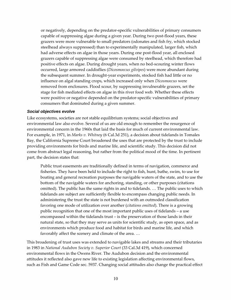
Figure 1.4. Variation in streamwise water velocity over 30 seconds, 10 cm from the bed in a pool in a stream in England. The heavy line shows a running average. Copied from Harvey and Clifford (2008). .................................................................................................................................. 18

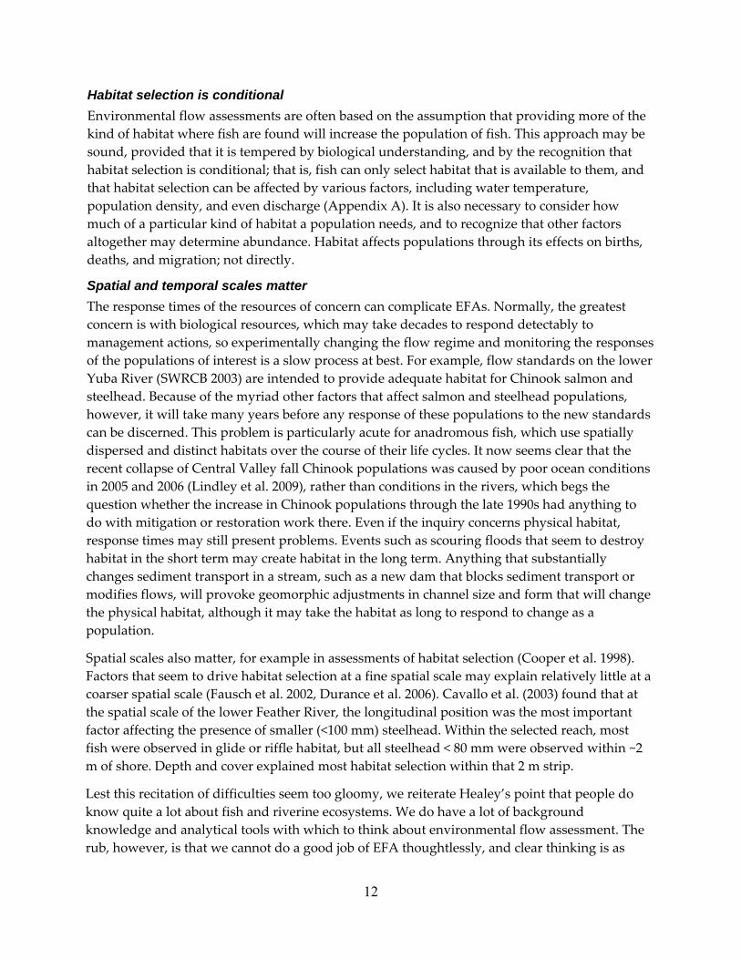
Figure 1.5. Velocity fluctuations measured 2 mm above a stone, using hot film anemometry. The velocity scale is cm per second. Copied from Figure 3 in Hart et al. (1996). ........................... 18

Figure 1.6. Rapid change in flow in the Big Sur River during and after a spring spate on April 4, 2010. The discharge before the spate was 170 cfs, and the peak discharge was 679 cf. Daily averaged flow, the statistic usually reported, conceals considerable variation. Data from USGS gage 11143000. ....................................................................................................................... 19

Figure 1.7. Annual variation in daily flow in Butte Creek, California, for water years 2000 to 2009 (dotted lines), plus mean (solid line). Even averaged over ten years, the annual hydrograph is not smoothed. ......................................................................................................... 19

Figure 1.8. Drawing of fish holding position in slow water adjacent to faster moving water. Copied from Stalnaker et al. (1996). .............................................................................................. 20

Figure 1.9. Schematic of trout swimming in four positions relative to an obstacle in the flow, seen from above. The top panel shows outlines of the fish, the obstacle, and flow lines; the bottom panel shows positions occupied by the dorsal centerline of the fish over time. In the Kármán gait (d) fish exploit the vortex sheets downstream of obstacles. Copied from Liao (2007). ................................................................................................................................................. 20

Figure 1.10. Brown trout holding in the lee of a submerged stone in Spruce Creek, Pennsylvania. Copied from Figure 10 in Bachman (1984). .................................................................................. 21

Figure 1.11. Conceptual model for the energetic benefit from drift feeding, as a function of water velocity. Copied from Hill and Grossman (1993). Capture efficiency declines as velocity increases about some threshold, reducing the benefit. ............................................................... 22

ix

Figure 1.12. The benefit or cost of drift feeding by small (53‐70 mm SL) rainbow trout as a function of velocity, in units of cm∙s‐1, modeled by Hill and Grossman (1993). Parameters for the estimate of benefit were developed from feeding experiments. ................................... 22

Figure 1.13. Computed tomography image of the pattern of activity in a human brain during a bilateral activity, such as typing the word ‘fish.’ Image from K. Sigvart, UC Davis. ............. 24

Figure 1.14. Area‐elevation curves for Butte, Mill and Deer creeks, for elevations above 200 m. These streams support the remaining independent populations of spring Chinook in the Central Valley. Note the steepness of the lower portion of Deer Creek, and the relatively low gradient, high elevation reach. Although it is the smallest of the three watersheds, Mill Creek extends to higher elevations on Mount Lassen than the other two. .............................. 25

Figure 1.15. A variety of images and figures derived from remote sensing data by the ALPS software, copied from Kinzel (2009); Clockwise from upper left: RGB imagery, color‐infrared imagery, laser raster, waveforms, flight line map, and first‐surface elevation map. ............................................................................................................................................................ 26

Figure 1.16. Local density of (a) baetid and (b) heptageniid mayflies across the stream bed in relation to near‐bed velocity. Data were analyzed statistically as limiting relationship using quantile regression; model lines indicate the 90th and 10th quantiles (upper and lower lines, respectively. Figure and legend copied from Lancaster and Downes (2010). ......................... 33

Figure 1.17. The horizontal component of the flow field near a boulder at base flow: a, as estimated by a 2‐D model; b, as estimated by a 4‐D model 11 cm from the bed; and c, as estimated by a 4‐D model 15 cm from the bed. The arrows show the magnitude and direction of the computed flow. The top of the boulder is above the surface of the water at this discharge. Copied from Shen and Diplas (2008). ................................................................. 37

Figure 1.18. (a) water velocity profile computed with a 4‐D model for a point about 0.1 m downstream from the boulder shown in Figure 1.17, at peak flow. The point of maximum velocity is circled. The vertical lines show the mean velocities estimated by the 4‐D model (0.89 m∙s‐1) and by the 2‐D model (1.08 m∙s‐1). (b) As in (a), but for a point about 2 m downstream from the boulder; stars show velocity measured with ADCP equipment. Copied from Shen and Diplas (2008). ........................................................................................... 38

Figure 1.19. Variation in width along the Nueces River, Texas, at low flow, determined from digital aerial photography by Fonstad and Marcus (2010), together with width estimated from downstream hydraulic geometry (DHG width). Copied from Figure 2 in Fonstad and Marcus (2010). ................................................................................................................................... 45

Figure 1.20. The relation between the number of [non‐salmonid] fish and the habitat index calculated by MesoHABSIM at 220 locations, using parameters estimated from samples the year before. Copied from Parasiewizc and Walker (2007). ........................................................ 49

Figure 1.21. Means and bootstrap 95% confidence intervals for juvenile WUA at 4.25 m3∙s‐1, for 50 samples of the Cache la Poudre River WUA curves, stratified by habitat type, with

x

sample sizes of 9, 28, and 55, and no errors. These show the variation that might be expected in the results of repeated applications of PHABSIM that were perfectly accurate except for transect sampling error. The dotted lines show the overall mean for the 107 curves from which the samples were drawn. Copied from Williams (2010a). ....................... 52

Figure 1.22. Cartoon of the conceptual model linking flow to fish that underlies most EFAs, copied from Hatfield et al. (2003). “Other impacts” and “Other ecological stuff” are acknowledged, but not really incorporated into the assessments. ........................................... 53

Figure 1.23. Average mass of under‐yearling brown trout, as a function of fish density, in four sections of Convict Creek, Mono County, under (a) observational conditions, and (b) experimental depletions and augmentations. Copied from Jenkins et al. (1999). .................. 54

Figure 1.24. Components and model linkages of IFIM, copied from Bovee et al. (1998). .............. 57

Figure 1.25. Sources of error in modeling, copied from Bovee et al. (1998). .................................... 57

Figure 1.26. Linkage of hydrological data to river cross‐sections: (a) discharge ranges for all flow components and corresponding water depths; (b) expanded detail of one bank …, with zones of riparian vegetation and other features which can be linked to different water levels. Figure and legend copied from King et al. (2003). .......................................................... 60

Figure 1.27. Conceptual model of the adaptive management cycle, copied from Healey et al. (2008). Note that ‘policy’ as used here may include taking some action. ................................ 61

Figure 1.28. Influence diagram showing the relationship between streamflow factors and expected fish abundance ................................................................................................................. 74

Figure 1.29. A simple Bayesian Network for an assessment using PHABSIM in the context of the IFIM. The network has not been parameterized, the probabilities of all states are shown as equal. (We use PHABSIM in this example because people are familiar with it, not because we recommend it.) ........................................................................................................................... 75

Figure 1.30. A simple Bayesian network showing factors that determine brown trout and rainbow trout density (mostly young‐of‐the‐year) in Martis Creek, California. Conditional probability tables associated with each node (i.e., variable) in the network were derived from data collected from 1979‐2008. .............................................................................................. 76

Figure 1.31. A simple Bayesian Network for primary and secondary productivity in a Sierran stream. ............................................................................................................................................... 77

Figure 1.32. A simple Bayesian Network for trout productivity in a Sierran stream. .................... 78

Figure 2.1. Big Creek No. 4 Hydroelectric Project decision pathways for flow modifications (Source: figure 4‐1 in SCE 2008). .................................................................................................. 119

Figure 3.1. Mean daily discharge (solid line) and maximum daily water temperature (dotted line) of Martis Creek, California for water years 1979‐2008. Gray shaded area represents the

xi

minimum and maximum recorded discharge for each day during the 30 years of study. Data are from USGS gage 10339400. ........................................................................................... 122

Figure 3.2. Annual mean (bars) and peak instantaneous (diamonds) discharge during each water year of study (1979‐2008). The horizontal dash line represents median discharge for the complete period of record (1974‐2008; USGS gage 10339400). Gray, hatched, and black vertical bars indicate wet (≥ 75th percentile), normal, and dry (≤ 25th percentile) water year types, respectively. Note log scale for instantaneous discharge. ............................................ 127

Figure 3.3. Relative abundances of key fish species during annual surveys of four permanent sample sites in Martis Creek, California, 1979‐2008. Alien fish are represented in plots A‐C while native fish are represented in plots D‐I. Sample sites 1 and 4 represent the downstream‐most and upstream‐most locations, respectively (see methods). .................... 130

Figure 3.4.Time series of density and biomass estimates for the Martis Creek fish assemblage, 1979‐2008. Bars (A, C) and circles (B, D) represent the annual mean (± 1 SE) of four sample stations. Black bars are mean values for the complete fish assemblage and gray bars are for native fishes only. No data were collected in 1986. Note log scale for plots A and C. ........ 133

Figure 3.5. Time‐lag and Bray‐Curtis distance of change in fish density (A) and detrended correspondence analysis (DCA) by year (B) for each sample site. Points represent differences in years for all year‐to‐year combinations plotted against Bray‐Curtis distance. Each node in the DCA biplot represents the fish assemblage in a given year. Years are connected by a line to illustrate change over time. ................................................................... 134

Figure 3.6. Results of the principal component analysis (PCA) performed on the correlation matrix of hydrologic variables presented in Table 3.2. Two ecologically interpretable axes accounting for 75.3% of the original variation were retained and included in multiple linear regression analyses. ....................................................................................................................... 135

Figure 3.7. Proportion of alien fish as a function of mean (A) and maximum (B) annual discharge, and frequency of flood events during winter (1 December ‐ 31 March) and spring (1 April ‐ 30 June) of each water year (C). P‐values are based on Spearman’s rank correlation (rs) for A and B and a quasi‐Poisson regression model for C. ............................. 137

Figure 4.1. Map of lower Putah Creek, Yolo and Solano counties, California, and fish sample sites. Key to sample site abbreviations: D = Putah Diversion Dam, I = Interstate 505, S = Stevenson Bridge Road, P =Pedrick Road, O = Old Davis Road, and M = Mace Boulevard. Figure modified from Marchetti and Moyle (2001). .................................................................. 145

Figure 4.2. Flow regime for Lower Putah Creek, California, USA. (A) Mean daily discharge from the Putah Diversion Dam during the period of study, 1991‐2008. Water year types (WYT) are defined as wet (W), above normal (AN), below normal (BN), dry (D) and critical (C). (B) Summary of discharge for each day of the water year based on the complete period of record (N = 31 years): solid line = mean discharge, gray shaded region = range of discharge values. .............................................................................................................................................. 146

xii

Figure 4.3. Two‐way cluster analysis of species abundances and sample events (sites and years) prior to implementation of the flow Accord, 1991‐1999. Species abbreviations used along the top of matrix are defined in Table 4.2. Native species are denoted with asterisks. Sample site codes (left side of matrix) are: D = Putah Diversion Dam, I = I‐505, S = Stevenson Bridge, P = Pedrick Rd., O = Old Davis Rd., M = Mace Blvd., followed by a two‐digit abbreviation for the sample year (e.g., 91 = 1991). ............................................................................................ 151

Figure 4.4. Two‐way cluster analysis of species abundances and sample events (sites and years) after implementation of the flow Accord, 2000‐2008. Species abbreviations used along the top of the matrix are defined in Table 4.2. Native species are denoted with an asterisk. Sample site codes (left) are followed by a two‐digit abbreviation for the sample year (e.g., 00 = 2000). Site codes are defined in Fig. 4.3. .............................................................................. 152

Figure 4.5. Non‐metric multidimensional scaling ordinations of the lower Putah Creek fish assemblages at six sites before (A) and after (B) alteration of the flow regime. Species scores were derived from log10(x+1) transformed abundances. Shaded ellipses represent the 95% confidence interval surrounding the mean position of each sample site in ordination space. Taxon codes are provided in Table 4.2. ....................................................................................... 153

Figure 4.6. Time series of annual total fish abundance, proportion of native species and taxon richness at each sample site, 1991‐2008. Gray shaded region indicates samples collected prior to implementation of the flow Accord in 2000. ................................................................ 157

Figure 4.7. Relationship between mean spring (1 March through 30 May) discharge and the proportion of the total fish assemblage comprised of native species at each sample site. Proportion data were arcsine square‐root transformed prior to regression analysis. ......... 157

Figure 4.8. Relationship between mean annual 7‐day maximum discharge and the proportion of the total fish assemblage comprised of native species at each sample site. Proportion data were arcsine square‐root transformed prior to regression analysis. ...................................... 158

xiii

List of Tables

Table 2.1. Hydropower licensing proceedings used to assess contemporary trends in environmental flow assessment and post‐license fisheries monitoring requirements. ......... 84

Table 2.2. Lower Feather River minimum flow requirements (cfs) downstream of the Thermalito Afterbay. Table modified from DWR (2007). ............................................................................... 85

Table 2.3. Documented fish species (current and historical) in each of the major areas affected by the Oroville Facilities, FERC Project No. 2100. ............................................................................ 86

Table 2.4. Fish species identified in waterways associated with the Pit 3, 4, 5 Hydroelectric Project. ............................................................................................................................................... 89

Table 2.5. Summary of minimum stream flows required in the bypassed stream reaches associated with Pit 3, 4, 5 (Source: FERC 2007a). ......................................................................... 91

Table 2.6. Existing minimum flow requirements (m3/s) to the bypassed reach from the El Dorado diversion dam (Source: FERC 2003a). ............................................................................. 93

Table 2.7. Fish species and their distribution in waters associated with the El Dorado Hydroelectric Project. ...................................................................................................................... 94

Table 2.8. Required minimum stream flows in the bypassed reach below Lake Isabella. ............ 98

Table 2.9. Instantaneous minimum stream flows required below the diversion in South Fork Willow Creek, Madera County, California. ............................................................................... 108

Table 2.10. Summary of instream flow assessment methods and new license conditions associated with each FERC project. ............................................................................................. 116

Table 2.11. Summary of frequency of fisheries monitoring required in new FERC licenses. ..... 117

Table 3.1. Characteristics of the four permanent sample sites (S1‐S4) in Martis Creek, California, 1979‐2008. Variables in boldface type were included in multiple linear regression models. .......................................................................................................................................................... 124

Table 3.2. Hydrological variables used to predict annual fish densities in Martis Creek, California, 1979‐2008. Predicted effects on native and alien species are classified as positive (+), weakly positive (0+), neutral (0), weakly negative (0–), negative (–), or strongly negative (– –). .................................................................................................................................................. 125

Table 3.3. Results of the Indicators of Hydrologic Alteration analysis for Martis Creek, California, 1979‐2008. Values are derived from non‐parametric regressions of hydrologic variables against time. ................................................................................................................... 128

Table 3.4. Frequency of occurrence of fish species during annual surveys of four permanent sample sites (S) in Martis Creek, California, 1979‐2008. The ‘all’ sites category indicates the number of years a species was found at all sample sites. ........................................................ 129

xiv

Table 3.5. Trend analysis (nonparametric Spearman’s rank correlation) of species densities and biomasses for the period 1979‐2008 at four sample stations in Martis Creek, California. Significant (P < 0.05) values are indicated in bold. .................................................................... 131

Table 3.6. Statistically significant change points derived from indexed annual species abundances, 1979‐2008. Solid circles indicate significant downturns in the population trajectory and open circles indicate significant upturns. Water year type (WYT) designations are dry (D), normal (N), and wet (W); see methods section for definitions. .. 132

Table 3.7. Coefficients of variation (%) of species density and biomass at each sample site in Martis Creek, California, 1979‐2008. ............................................................................................ 132

Table 3.8. Results of stepwise multiple linear regression analysis using species density as the dependent variable. Data were transformed prior to analysis. PC1 and PC2 were derived from principle component analysis of flow attributes. Higher PC1 values can be interpreted as lower annual discharge (dry water years). PC2 relates to seasonality of peak flows with positive values indicating high flow events earlier in the water year (i.e., winter) and negative values indicating late season (spring) spates. A second set of regression models which included brown trout density as a proxy for brown trout predation did not change the results for any species. ............................................................................................................ 136

Table 4.1. Results of the Indicators of Hydrologic Alteration analysis for lower Putah Creek contrasting select attributes of the flow regime before and after alteration of the flow regime. ............................................................................................................................................. 149

Table 4.2. Fish species collected at six permanent sample sites in lower Putah Creek, California, USA. ................................................................................................................................................. 150

Table 4.3. Matrix of A‐values derived from multi‐response permutation procedure (MRPP) contrasting the fish assemblages at six sample before (upper‐half of matrix) and after (lower‐half of matrix) alteration of the flow regime. ................................................................ 155

Table 4.4. Indicator value (IV) scores and associated P‐values obtained by Monte Carlo permutations for fish taxa at the 6 permanent sample sites. Indicator species were determined separately for the pre‐ (1991‐1999) and post‐Accord (2000‐2008) periods. ...... 156

xv

xvii

Abstract

California faces a wave of licensing of dams for power production, with approximately half of the dams scheduled to be licensed over the next 15 years. The number of projects, the cost of the licensing process, and the increased appreciation of the complexity of stream ecosystems, highlight the need for better methods for determining how much water should to be left in the streams, using Environmental Flow Methodologies. The authors examined the range of methods available assessing environmental flows in relation to Federal Energy Regulatory Commission (FERC) licensing processes in California. We specifically sought to integrate insights from allied fields not usually applied to environmental flow methodologies. A particular goal was to see if environmental flow methodologies in use in California are consistent with generally accepted practice in the scientific community, especially in their statistical approaches to problems. The researcher’s basic findings include: (1) environmental flow methodologies used most frequently in California are seriously flawed, including their underlying statistical foundations; (2) alternatives are available (e.g., using Bayesian Networks) that are both more effective and likely less costly; (3) The fish assemblages of California streams have a complex relationship to flows but it is possible to manage regulated streams to favor desired fish assemblages (e.g., endemic fishes); (4) Required monitoring programs for Federal Energy Regulatory Commission projects are generally inadequate and, as a result, have a high probability of leading to erroneous conclusions about the effects of projects on fish populations. The overall results of this research indicate that the efficiency and effectiveness of environmental flow evaluations can be increased, while reducing their costs and providing benefits to both fish and water users. Specific suggestions for improving environmental flow methodologies are provided.

Keywords: environmental flow methodologies, Bayesian Networks, Instream Flow Incremental Methodology, Physical Habitat Simulation System, environmental flow assessments, flow regime, Federal Energy Regulatory Commission.

Executive Summary

Introduction

California faces a wave of (re)licensing of dams for power production, with approximately half of the dams scheduled to be licensed over the next 15 years. The present wave of licensing provides an opportunity to develop a better balance between power generation and stream ecosystem function. The sheer number of projects, the cost of the licensing process, and the increased appreciation of the complexity of stream ecosystems, highlight the need for better methods for determining how much water should to be left in the streams. This project, therefore, deals with evaluating existing Environmental Flow Methodologies used in California, especially from the perspectives of scientific validity, effectiveness in application to the state’s distinctive hydrology, and effectiveness in accomplishing stated goals.

Project Objectives

The authors examined the range of methods available assessing environmental flows in relation to Federal Energy Regulatory Commission (FERC) licensing processes in California and specifically sought to integrate insights from allied fields not usually applied to environmental flow assessments. A particular goal was to see if environmental flow methodologies in use in California are consistent with generally accepted practice in the scientific community, especially in their statistical approaches to problems and investigated ways to improve evaluating environmental flows. More specific objectives that were accomplished include:

• Conducting an expanded literature review, beyond what has already been done, focusing on non‐traditional methods that could be applied to environmental flow methodologies;

• As a result of the literature review, providing a guidance document for participants in Federal Energy Regulatory Commission processes;

• Examining the long‐term variability in flows in two regulated streams (Martis Creek, Putah Creek) with annual data, to gain an understanding of results that would be likely if monitoring of the effectiveness of environmental flow methodologies was performed at greater intervals than one year;

• Conducting a retrospective analysis of the monitoring programs required under recent Federal Energy Regulatory Commission licensing agreements for their likely effectiveness.

The overall results of this research indicate that the efficiency and effectiveness of environmental flow evaluations can be increased, while reducing their costs and providing benefits to both fish and water users.

Project Outcomes

Chapter 1: Environmental Flow Assessments: A Critical Review and Commentary

Environmental flow assessment remains an extraordinarily difficult problem, for which no existing methods provide a defensible technical solution; this makes an adaptive approach with careful attention to uncertainty appropriate. The difficulties with

1

environmental flow assessments spring from the complexity and variability of stream ecosystems, so improved understanding of stream ecosystems and aquatic organisms will be a critical component of a long‐term resolution of the problem. Nevertheless, substantial improvements in the state of practice are possible in the short‐term in several ways: (1) technological improvements in collecting, displaying and analyzing physical data on stream ecosystems allow for more accurate representations of the systems in environmental flow assessments; (2) proper attention to sampling can improve the accuracy of estimates developed from field studies, and allow for reporting interval estimates rather than point estimates; (3) Bayesian hierarchical modeling can allow for modeling more complex problems than was possible with other statistical methods; (4) Bayesian Networks have emerged as a promising framework for dealing with complex problems such as environmental flow assessments.

Chapter 2: Retrospective Analysis of Environmental Flows and Fish Monitoring in Federal Energy Regulatory Commission Licensing

In this chapter the authors reviewed thirteen recent FERC hydropower licensing proceedings in California. The purpose was to assess if fish monitoring requirements were routinely mandated in new Federal Energy Regulatory Commission licenses and how useful the information collected was likely to be in determining effects of the dams. It was found that nearly all new licenses included conditions requiring minimum instream flow releases. While changes to release flows were commonplace, only 8 (62%) of the projects examined contained language in the new license mandating fish monitoring over the term of the license. Of those 8 projects, sampling requirements ranged from a single post‐license survey up to 12 surveys over a 40‐year term. Management objectives for fishes in hydropower‐affected waterways, when stated, were commonly the maintenance of some level of abundance similar to levels determined from previous surveys. However, given the natural variability inherent in stream populations, the authors believe performance criteria based on fish density or size have the potential to lead to spurious conclusions, even when rigorous statistical methods are applied.

Chapter 3: Factors Affecting the Fish Assemblage in a Sierra Nevada, California, Stream

The fishes of Martis Creek, in the Sierra Nevada of California, were sampled at 4 sites annually for 30 yrs, 1979‐2008. This long‐term data set was used to examine the hypotheses that (1) the fish assemblage is persistent and resilient through time, (2) native and alien (non‐native) fishes respond differently to the flow regime, and (3) the principal determinant of fish assemblage composition is flow regime. Annual changes in fish density and biomass were related to 14 attributes of the flow regime, as well as to 13 habitat variables. Despite high inter‐annual variability in mean and peak discharge values, the basic character of flow regime did not change over the period of study. Fish assemblages were persistent at all sample sites but had marked inter‐annual variability in density and biomass. Most native fishes declined while most alien species showed no

2

trends. Abundances of native species were tied mostly to habitat variables, while alien species responded to flow magnitude and timing/duration, especially brown trout. Frequency of high‐flow events had a negative relationship on proportion of alien species. The results indicate the need for continuous annual monitoring of streams with altered flow regimes, as well as to have monitoring of relatively unaltered streams for comparison. Apparent successes or failures in flow management may appear in a different light under long‐term study

Chapter 4: Restoring Native Fish Assemblages to a Regulated California Stream Using the Natural Flow Regime Concept

In this chapter, an empirical example is provided of how changes to the flow regime successfully re‐established native fishes and reduced abundances of alien fishes in a regulated California river (lower Putah Creek; Yolo and Solano counties). A series of wet water years, followed by implementation of a flow regime specifically designed to benefit native species, produced dramatic shifts in the distribution and abundance of fishes. The native cold‐water fish assemblage that was previously restricted to habitat immediately below Putah Diversion Dam expanded downstream more than 6 km. Additionally, native Sacramento pikeminnow, Sacramento sucker, tule perch, and hitch that collectively represented a minor proportion of the total fish assemblage in middle reaches of lower Putah Creek before the new flow regime, have since become the numerically dominant taxa. These results demonstrate that natural flow regimes can be used to effectively manage and enhance fish assemblages in regulated rivers. Further, this study underscores the importance of long‐term quantitative fish monitoring programs to assess the outcomes of management actions.

Conclusions and Recommendations

The author’s basic findings include: (1) environmental flow methodologies used most frequently in California are seriously flawed, including their underlying statistical foundations; (2) alternatives are available (e.g., using Bayesian Networks) that are both more effective and likely less costly; (3) The fish assemblages of California streams have a complex relationship to flows but it is possible to manage regulated streams to favor desired fish assemblages (e.g., endemic fishes); (4) Required monitoring programs for Federal Energy Regulatory Commission projects are generally inadequate and, as a result, have a high probability of leading to erroneous conclusions about the effects of projects on fish populations. The authors therefore recommend that environmental flow assessments associated with Federal Energy Regulatory Commission proceedings should be held to strict standards of scientific accountability, including statistical reliability. This means that different methods are likely necessary other than those currently in use (such as the Instream Flow Incremental Methodology [IFIM] and /or the Physical Habitat Simulation System [PHABSIM]). Such methods are either already available or possible to develop using existing analytical techniques (for example, Bayesian Networks). Part of the improved assessments needed is better, typically more frequent, monitoring. For most projects, annual monitoring should be conducted (pre and post project) until project effects can

3

be determined through both wet and dry periods. Once sufficient data is available, a realistic adaptive monitoring program can be developed that would occur through the life of the project.

Benefits to California

The overall results of this research indicate that the efficiency and effectiveness of environmental flow evaluations can be increased, while reducing their costs and providing benefits to both fish and water users. The benefits to California include better predictions of project environmental effects, which can improve fish populations at minimal costs to project operations, perhaps even resulting in cost savings.

4

1.0 Environmental Flow Assessments: A Critical Review and Commentary John G. Williams, Center for Watershed Sciences, University of California, One Shields Avenue, Davis, CA 95616, [email protected]

1.1. Introduction California faces a wave of relicensing of dams for power production, with approximately half of the dams scheduled to be relicensed over the next 15 years. Because most of the original licenses were granted 30 to 50 years ago, when there was less concern for and knowledge of the impacts of the projects on stream ecosystems, the present wave of relicensing provides an opportunity to develop a better balance between power generation and stream ecosystem function. The sheer number of projects, the cost of the relicensing process, and the increased appreciation of the complexity of stream ecosystems, highlight the need for better methods for determining how much water should to be left in the streams. In response to this need, the California Energy Commission (CEC) has funded several projects that aim to improve such methods, through the Instream Flow Assessment Program of the Center for Aquatic Biology and Aquaculture of the University of California, Davis. This review is part of one these projects.

This review of methods for instream or environmental flow1 assessment (EFA) is intended to assist people who work on the problem of how much water should be left in streams to maintain aquatic ecosystems, or species of particular concern or legal status. We refer to these methods as environmental flow methods (EFMs), to distinguish the methods from the overall process in which they are applied. If this seems confusing, consider that a single EFA could use multiple EFMs. There is a very large literature on EFMs, and competent reviews of much of it have been published by others (e.g., EPRI 2000, Tharme 2003, Hatfield et al. 2003, Annear et al. 2004). There is little point to duplicating this work, so instead we will use it as a point of departure for a critical review and evaluation of current approaches that will emphasize concepts and methods from other areas of science, such as ecology, statistics, and wildlife management that could be, but generally are not, integrated into environmental flow assessment. We assume that people reading this report will be reasonably familiar with existing EFMs and the regulatory and political contexts in which they are normally applied. Those who are not should first read one of the reviews listed above; we recommend EPRI (2000) or Hatfield et al. (2003), which are available on the web,2 followed by Tharme (2003), which provides an international perspective.

There is normally a trade‐off in reviews between being comprehensive and complete and being tedious and boring. We have tried to make the main text readable by putting some of the more 1 We prefer “environmental flows” to “instream flows,” because the former more accurately reflects the rationale for setting flow targets in regulated rivers and avoids confusion with the Instream Flow Incremental Methodology (IFIM). 2 Search for Hatfield et al. (2003) by its title; for EPRI (2000), search by the document number, TR‐1000554, in the ‘search’ box on the EPRI website.

5

detailed material in appendices. We are also mindful of the practical constraints within which EFAs normally must be carried out, and have tried to make our suggestions realistic, but we do not accept that the best that can be done within the constraints must therefore be good enough. We do not expect EFMs to be flawless, but they should meet ordinary norms for scientific or regulatory practice, and, critically, shortcomings should be disclosed. Because our focus here is on methods useful for the FERC licensing process, we assume that some resources will be available for considering each affected stream individually. Therefore, we mention but do not emphasize methods or approaches such as ELOHA (Poff et al. 2010) that are designed for regional applications, especially in resource‐scarce situations. Similarly, to keep the task manageable we have focused on EFMs related directly to organisms in streams, and have mostly ignored other important factors such as the role of high flows for habitat creation or maintenance, and the role of riparian and terrestrial habitats as sources for nutrients or large wood. That is, we assume that some ‘holistic’ approach will be taken, and focus on the part dealing directly with aquatic animals.

To make the review relevant, we have tried to address at least the spirit of the concerns raised by people involved with FERC processes that are described in Cox (2007). As summarized in the executive summary of that document (Cox 2007 vii):

Stakeholders saw a need for studies that would: a) encourage increased consistency of hydropower licensing study protocols, and b) compare and contrast standard environmental flow assessment methods with a number of less‐well‐known, but promising, new approaches. Stakeholders also cited a need for ecological research to fill gaps in scientific understanding of instream flows, including research aimed at refining habitat and temperature management for a range of species.

The structure of this review is as follows. Section 1.2 covers some background considerations for EFA, intended mainly to explain why the problem of assessing the effects of water management is so difficult. Section 1.3 discusses the complexity of flow in streams, how it is measured, and how drift‐feeding fish and flow interact. Section 1.4 describes methods or concepts that can be used in EFMs – the pieces of which EFMs are made. Section 1.5 reviews EFMs and frameworks for EFAs, and gives summary reviews of other reviews of EFMs. Section 1.6 elaborates on the use of Bayesian Networks, an approach that is being applied in Australia that we think could improve assessments here, and help provide the consistency that stakeholders would like. Section 1.7 gives summary conclusions and recommendations.

On a technical point, many of the recent articles we consider were published online in one calendar year and in print the next. We have opted to cite the date of the printed version, but warn that the same articles may be cited differently elsewhere.

6

1.2. Background Considerations 1.2.1. Why is this so hard? Fourteen years ago, several of us participated in a small workshop on environmental flow assessment at the University of California at Davis, in which we concluded that “…currently no scientifically defensible method exists for defining the instream flows needed to protect particular species of fish or aquatic ecosystems” (Castleberry et al. 1996). Despite considerable effort by many and significant progress over the last 15 years, we still believe that this is the case; the best that can be done is still best regarded as a first cut that should be implemented within the context of adaptive management. Why is this problem so hard? Scientists have a truly wonderful understanding of the nature of energy and matter, the evolution of the universe, the atomic structure and properties of molecules, the structure and activities of cells, the origin of species and the evolutionary relationships among organisms, and much more. Why, then, is it so hard to assess the consequences of taking some of the water out of a stream, or changing the timing with which water flows down the stream? One answer to this question has been given by Mike Healey, formerly the lead scientist for the CALFED Bay‐Delta Authority, in the final chapter in a book on river ecology and management (Healey 1998:666‐667):

What can and cannot be known about watershed ecosystems?

Our daily confrontation with the ecological naiveté of traditional river and watershed management seems to belie the scholarly contents of this and other recent publications on ecology and river management (Gore and Petts 1989, Calow and Petts 1992, Naiman 1992). The preceding chapters clearly demonstrate the accumulating wealth of technical information about rivers and their catchments. Such knowledge is not simply an encyclopedia of unconnected facts. A growing list of integrating concepts ‐ the river continuum concept (Vannote et al. 1980), the flood pulse concept (Junk et al. 1989), the serial discontinuity concept (Ward and Stanford 1983), the riverine productivity concept (Thorp and Delong 1994) ‐ provide structure to the facts and a rich intellectual framework for speculating about the response of catchments to human activity. Yet, this wealth of knowledge about rivers has not paved the way to ecosystem management. The key to ecosystem management may lie in further research and study. This argument is particularly appealing to those who see ecosystem and environmental management primarily as a technical problem. Paradoxically, however, the problem posed by ecosystems and by watersheds as particular examples of ecosystems is at once both a technical problem and a problem that is not resolvable by technological means.

This apparent paradox arises from two important and possibly interrelated features of ecosystems. The first of these is that ecosystems are “medium number” systems (O’Neill et al. 1986). That is to say, ecosystems are made up of a moderate number (a few hundred to a few thousand) of interacting subsystems. It is virtually impossible to predict the future states of such a system when it is disturbed. The number of interactions is too large for straightforward analytical solution (as with the behavior of planets in a solar system) and too small to be smoothed out through some emergent law

7

of averages (as the behavior of molecules in a vessel of gas is averaged in the gas laws). Attempting to resolve the behavior of ecosystems through the study of their interacting subsystems is rather like trying to discover the gas laws by studying the behavior of individual molecules.

The second feature is that ecosystems display patterns suggestive of chaotic behavior (Schaffer 1985). Whether ecosystem behavior is truly chaotic remains to be resolved. Nevertheless, ecosystems are characterized by “surprise” events on a wide range of time and space scales (Holling 1987, 1992, Healey 1990, Costanza et al. 1993). Rivers are the embodiment of dynamic hydrological forces operating within a heterogeneous and complex physical matrix (their “catchment”). They are particularly likely to deliver dramatic surprises, including floods, abrupt channel shifts, and debris torrents, all of which have associated ecological consequences.

This “unknowable” character of rivers and river basins is part of their fascination as ecosystems. But their “unknowableness” also means it is not possible to predict their behavior the way that the behavior of structural materials in a bridge or the airfoil of a jet plane can be predicted. Fortunately, this does not mean that the goal of ecosystem management must be abandoned. What is does mean is that approaches to the management of ecosystems must differ from approaches to the management of traffic on highways or to the exploitation of individual fish populations. In the latter two instances, management is based on simple analytic models that predict quantities (e.g., vehicles, fish) that can be accommodated or harvested in a specified period of time. Such quantitative statements about ecosystem behavior may never be possible. Questions about the quantitative behavior of ecosystems are typically of the sort that Weinberg (1972) termed “transscientific.” These are questions that can be framed in the language of science but cannot be answered by the traditional means of science. A familiar example of such a transscientific question about a river ecosystem is: “How much can a river’s hydrology be altered without endangering its ecological integrity?” This question is at the heart of the ongoing debate about in‐stream flows for fish and other aquatic life. Notwithstanding increasingly elaborate attempts to provide a technical solution (Walder 1996), the question is not soluble by traditional reductionist science. It is not soluble because the solution demands orderliness and a consistency of behavior of riverine ecosystems that does not exist. Such questions can only be answered in terms of relative risk to ecological integrity with different models or approaches often giving different results.

1.2.2. The many challenges Whether one accepts that EFA is transscientific or not, there are formidable challenges to analyzing the effects of changes in hydrological regimes on stream ecosystems.

Ecosystems are not stable equilibrium systems This point, touched on by Healey (1998), was elaborated in the consensus report of a major conference on the management of wild living resources (Mangel et al. 1996):

8

In the early 1970s most resource managers behaved as if it were possible to manage the use of living resources in a relatively sustainable and predictable way: the only questions was how to achieve that sustainable yield. The philosophy was that each resource had a maximum or optimum sustainable yield level and that the measurement and calculation of the appropriate levels were feasible if enough natural history and demography were known. Thus, resource conservation was regarded primarily as a biological problem, and the key to maximum sustained use was information about the species or stocks and their ecosystems, as well as analysis of biological data to develop appropriate regimes. … The perspective today is far different. (p. 339). …

Formerly, the dominant paradigm was that of an ecosystem that was stable, closed, and internally regulated and that behaved in a deterministic manner. The new paradigm is of a much more open system, one that is in a constant state of flux, usually without long‐term stability, and affected by a series of human and other, often stochastic, factors, many originating outside the of the ecosystem itself. As a result, the ecosystem is recognized as probabilistic and multi‐causal rather than deterministic and homeostatic; it is characterized by uncertainty rather than the opposite. Two types of uncertainty are involved in living‐resource conservation. The first could be considered “ecological uncertainty,” which refers to the probabilistic nature of biological systems discussed in the previous paragraph. The second type is uncertainty in the estimation of parameters such as abundance, birth and death rates, etc.; this is “measurement uncertainty.” Both of these types of uncertainty are central concerns to any model or management regime, but there is often confusion between them when uncertainty is discussed. (p. 356)

Ecological uncertainty is well demonstrated by a long‐term study on the South Fork Eel River in Northern California (Power et al. 2008:263); although the highly predictable seasonality of flow is a major factor structuring the food web there, year to year variation in the timing and magnitude of high flow events results in substantial variation in the structure of the food web and its response to mobilization of the bed by high flows.

Eighteen years of field observations and five summer field experiments in a coastal California river suggest that hydrologic regimes influence algal blooms and the impacts of fish on algae, cyanobacteria, invertebrates, and small vertebrates. In this Mediterranean climate, rainy winters precede the biologically active summer low‐flow season. Cladophora glomerata, the filamentous green alga that dominates primary producer biomass during summer, reaches peak biomass during late spring or early summer. Cladophora blooms are larger if floods during the preceding winter attained or exceeded ‘‘bankfull discharge’’ (sufficient to mobilize much of the river bed, estimated at 120 m3/s). In 9 out of 12 summers preceded by large bed‐scouring floods, the average peak height of attached Cladophora turfs equaled or exceeded 50 cm. In five out of six years when flows remained below bankfull, Cladophora biomass peaked at lower levels. Flood effects on algae were partially mediated through impacts on consumers in food webs. In three experiments that followed scouring winter floods, juvenile steelhead (Oncorhynchus mykiss) and roach (Lavinia (Hesperoleucas) symmetricus) suppressed certain insects and young‐of‐the‐year fish fry, affecting persistence or accrual of algae positively

9

or negatively, depending on the predator‐specific vulnerabilities of primary consumers capable of suppressing algae during a given year. During two post‐flood years, these grazers were more vulnerable to small predators (odonates and fish fry, which stocked steelhead always suppressed) than to experimentally manipulated, larger fish, which had adverse effects on algae in those years. During one post‐flood year, all enclosed grazers capable of suppressing algae were consumed by steelhead, which therefore had positive effects on algae. During drought years, when no bed‐scouring winter flows occurred, large armored caddisflies (Dicosmoecus gilvipes) were more abundant during the subsequent summer. In drought‐year experiments, stocked fish had little or no influence on algal standing crops, which increased only when Dicosmoecus were removed from enclosures. Flood scour, by suppressing invulnerable grazers, set the stage for fish mediated effects on algae in this river food web. Whether these effects were positive or negative depended on the predator‐specific vulnerabilities of primary consumers that dominated during a given summer.

Social objectives evolve Like ecosystems, societies are not stable equilibrium systems; social objectives and environmental law also evolve. Several of us are old enough to remember the resurgence of environmental concern in the 1960s that laid the basis for much of current environmental law. For example, in 1971, in Marks v. Whitney (6 Cal.3d 251), a decision about tidelands in Tomales Bay, the California Supreme Court broadened the uses that are protected by the trust to include providing environments for birds and marine life, and scientific study. This decision did not come from abstract legal reasoning, but rather from the political mood of the time. In pertinent part, the decision states that:

Public trust easements are traditionally defined in terms of navigation, commerce and fisheries. They have been held to include the right to fish, hunt, bathe, swim, to use for boating and general recreation purposes the navigable waters of the state, and to use the bottom of the navigable waters for anchoring, standing, or other purposes (citations omitted). The public has the same rights in and to tidelands. … The public uses to which tidelands are subject are sufficiently flexible to encompass changing public needs. In administering the trust the state is not burdened with an outmoded classification favoring one mode of utilization over another (citations omitted). There is a growing public recognition that one of the most important public uses of tidelands – a use encompassed within the tidelands trust – is the preservation of those lands in their natural state, so that they may serve as units for scientific study, as open space, and as environments which produce food and habitat for birds and marine life, and which favorably affect the scenery and climate of the area. …

This broadening of trust uses was extended to navigable lakes and streams and their tributaries in 1983 in National Audubon Society v. Superior Court (33 Cal.3d 419), which concerned environmental flows in the Owens River. The Audubon decision and the environmental attitudes it reflected also gave new life to existing legislation affecting environmental flows, such as Fish and Game Code sec. 5937. Changing social attitudes also change the practical effect

10

of environmental laws. Monticello Dam on Putah Creek releases water for re‐diversion 10 km downstream; these releases support a trout fishery, which, together with recreational uses of the reservoir, was long thought to meet any environmental obligations arising from the project, including Fish and Game Code sec. 5937. Over time, however, native fishes that were formerly regarded as “trash fish” came to be valued, and litigation resulted in revised environmental flow releases to protect them (Moyle et al. 1998).

Fish evolve We are used to thinking of evolution as a slow process, but this is not always the case. According to Sterns and Hendry (2004), “A major shift in evolutionary biology in the last quarter century is due to the insight that evolution can be very rapid when populations containing ample genetic variation encounter strong selection (citations omitted).” It is now clear that significant evolution can occur within the period of a FERC license, and fish populations may respond to changes in the environment in unexpected ways. For example, in several Central Valley Rivers, releases of hypolimnetic water from reservoirs have created have good habitat for large trout. The steelhead populations in these rivers apparently have evolved toward a resident life‐history (Williams 2006). Where hatcheries “mitigate” for habitat lost above dams, fish evolve greater fitness for reproduction in hatcheries, and lower fitness for reproducing in rivers (Myers et al. 2004, Araki et al. 2007, 2008).

Streams adjust Alluvial or partially alluvial streams create their own channels. Anything that substantially changes flow or sediment transport in a stream, such as a new dam, will provoke geomorphic adjustments in channel size and form that will change the physical habitat, and the change may continue beyond the duration of a FERC license. For example, the Carmel River is still adjusting to changes in the sediment regime caused by dams built in 1921 and 1948 (Kondolf and Curry 1986, Larry Hampson, MPWMD, pers. comm. 2009).

Climate changes Long‐term climate records and paleoclimatic data from tree rings and other sources show that climates have always varied over decades and centuries, and now greenhouse gas emissions will drive change rapidly. One predictable change, already evident in flow data, will be more winter runoff and less snowmelt runoff in Sierran streams. Precipitation may also become more variable. Thus, the amount and temporal distribution of water available to be allocated between instream and consumptive uses will change, as will the temperature of the water. Predicting climate change at any particular location is even more difficult than predicting global change, so uncertainty about climate will add substantially to the uncertainties already faced in EFAs.

Fish populations vary Fish populations can be highly variable (e.g., Dauwalter et al. 2009), even in stable stream environments (Elliott 1994). This makes it difficult to determine population trends or whether changes in environmental flows have done any good or harm (Korman and Higgins 1997, Williams 1999). This is particularly true for anadromous fish, for which populations may be strongly affected by ocean conditions that vary from year to year (e.g., Lindley et al. 2009).

11

Habitat selection is conditional Environmental flow assessments are often based on the assumption that providing more of the kind of habitat where fish are found will increase the population of fish. This approach may be sound, provided that it is tempered by biological understanding, and by the recognition that habitat selection is conditional; that is, fish can only select habitat that is available to them, and that habitat selection can be affected by various factors, including water temperature, population density, and even discharge (Appendix A). It is also necessary to consider how much of a particular kind of habitat a population needs, and to recognize that other factors altogether may determine abundance. Habitat affects populations through its effects on births, deaths, and migration; not directly.

Spatial and temporal scales matter The response times of the resources of concern can complicate EFAs. Normally, the greatest concern is with biological resources, which may take decades to respond detectably to management actions, so experimentally changing the flow regime and monitoring the responses of the populations of interest is a slow process at best. For example, flow standards on the lower Yuba River (SWRCB 2003) are intended to provide adequate habitat for Chinook salmon and steelhead. Because of the myriad other factors that affect salmon and steelhead populations, however, it will take many years before any response of these populations to the new standards can be discerned. This problem is particularly acute for anadromous fish, which use spatially dispersed and distinct habitats over the course of their life cycles. It now seems clear that the recent collapse of Central Valley fall Chinook populations was caused by poor ocean conditions in 2005 and 2006 (Lindley et al. 2009), rather than conditions in the rivers, which begs the question whether the increase in Chinook populations through the late 1990s had anything to do with mitigation or restoration work there. Even if the inquiry concerns physical habitat, response times may still present problems. Events such as scouring floods that seem to destroy habitat in the short term may create habitat in the long term. Anything that substantially changes sediment transport in a stream, such as a new dam that blocks sediment transport or modifies flows, will provoke geomorphic adjustments in channel size and form that will change the physical habitat, although it may take the habitat as long to respond to change as a population.

Spatial scales also matter, for example in assessments of habitat selection (Cooper et al. 1998). Factors that seem to drive habitat selection at a fine spatial scale may explain relatively little at a coarser spatial scale (Fausch et al. 2002, Durance et al. 2006). Cavallo et al. (2003) found that at the spatial scale of the lower Feather River, the longitudinal position was the most important factor affecting the presence of smaller (<100 mm) steelhead. Within the selected reach, most fish were observed in glide or riffle habitat, but all steelhead < 80 mm were observed within ~2 m of shore. Depth and cover explained most habitat selection within that 2 m strip.

Lest this recitation of difficulties seem too gloomy, we reiterate Healey’s point that people do know quite a lot about fish and riverine ecosystems. We do have a lot of background knowledge and analytical tools with which to think about environmental flow assessment. The rub, however, is that we cannot do a good job of EFA thoughtlessly, and clear thinking is as

12

hard to do as it is essential. Therefore, we should do the best we can, be clear about what we did and did not do and why, and try to work in an adaptive framework that will allow changes in management as new information becomes available.

Other background considerations Science and dispute resolution: Environmental flow assessments almost always occur within the context of disputes over water, and the resolution of these disputes will involve trade‐offs and balancing, and often negotiation. For this reason, the main USGS publication on the use of the Instream Flow Incremental Methodology (Bovee et al. 1998) deals extensively with negotiation and dispute resolution. We do not deal with these aspects of the flow‐setting process in this review, since we are not experts at them, although we recognize that effective negotiation and dispute resolution are critical aspects of protecting environmental flows, and have taken this into account in our recommendations. However, it is also important to keep in mind that science and dispute resolution are separate endeavors that have different rules for settling questions. Distinctions among human activities often break down in the details, but generally, science settles questions by testing hypotheses or models with data. Procedures for doing this may be generally agreed upon, but they are always subject to criticism and alternatives can always be put forward, and conclusions are always subject to change in light of new evidence. In legal or political disputes, on the other hand, questions can also be settled by the parties agreeing to an answer, and in legal disputes this answer may be final, at least for the parties involved, regardless of new evidence that may emerge. For example, the parties in a dispute over water may agree that the results of a study of part of the stream in question will be applied to the whole. This will not wash in science. Science and dispute resolution both have major roles in EFA, but it is important to keep them separate.

In the regulatory world, disputes must be resolved, which requires that decisions be made in reasonable time, and this produces a tension between science and dispute resolution. Adaptive management, discussed in section 1.5, can be viewed as a way to reduce this tension, but it is unrealistic to think it will do away with it.

Models and environmental flow assessment: Models are important tools for environmental flow assessment, but they are often misused. The proper use of models is to help people think, not to think for them, or to provide them with “answers.” Inevitably, models embody simplifications of the world, based on the aspects of the world that we (or someone) believe are important for the problem at hand. That is, we model the way that we think the world works, but we should remember that the world has no obligation to work that way. The invaluable thing that models do is to show us the logical consequences of our thinking, or, for estimation models, to show us whether data support our thinking.

Objective and subjective methods: A few decades ago, it was common for scientists to promote “objective” methods for analyzing problems, generally by application of some numerical model. This conceit has largely been given up, in the face of persuasive arguments that modeling always involves subjective choices. For example, seemingly objective tests of statistical significance depend upon a subjectively chosen criterion for significance, such as α = 0.05. In modeling for EFAs, there are always subjective choices about what to include in the model and

13

how to do so (Kondolf et al. 2000). Subjectivity will enter into EFAs, whether we want it to or not; the question is whether the subjectivity will be recognized and taken into account.

Science and environmental flow assessment: For at least two reasons, described above, environmental flow assessment is not just science: the main question it asks is transscientific, and usually the question is asked in the context of dispute resolution. Science can and should inform environmental flow assessment, and EFMs should be consistent with scientific practice. However, the limits to what science can contribute should be recognized. Ecosystems are enormously complicated, and it is not realistic to expect that standard methods can be devised by which EFA can be successfully accomplished without good data, careful thought and informed judgment.

Just as science should inform EFAs, EFAs should inform science. That is, there should be feedback regarding questions and uncertainties that loom large in assessments, which may amenable to traditional scientific inquiry. Thus, the reasoning and assumptions underlying EFMs should be stated explicitly, as should the reasoning underlying environmental flow decisions. In particular, it should be possible to tell what kinds of evidence or new understanding would cause a change in the assessment or the decision.

1.2.3. A comment on the literature(s) There are several literatures on environmental or instream flow assessments or on matters highly relevant to them. It is common to distinguish peer‐reviewed journals and agency or consulting reports, but there are also important distinctions among peer‐reviewed journals. Roughly, there is a more academically oriented literature, largely in ecological journals, and a fisheries literature, with much of the surprisingly small overlap in the Canadian Journal of Fisheries and Aquatic Sciences and the Transactions of the American Fisheries Society. There are also many relevant papers in geomorphology, engineering, and statistics, and a large literature on habitat selection in wildlife journals. These distinctions matter, because the quality of the reviewing tends to vary. Generally, the reviewing for the academically more prestigious journals is more rigorous, but the reviewers for these journals may not be as familiar with the details of a particular topic as reviewers for the relevant specialty journals. Peer review is an important part of scientific quality control, but it is far from perfect, and many deeply flawed articles are published. The distinction that really matters is whether journal articles or agency reports are based on good logic and evidence.

14

1.3. Flow in Streams 1.3.1. Introduction Environmental flow assessment is about flow in streams or rivers, so we begin with a discussion of flow and how it varies over space and time, and. Flow in natural channels is usually turbulent, so the velocity fields3 in natural channels are highly complex. Even if the discharge is constant, the velocity at a given point in a stream can be highly variable over a range of time‐scales, and the velocity at any given instant can vary strongly over short distances. This makes just measuring the flow field as actually experienced by a fish a challenge, and modeling this complexity is an even greater challenge. Some examples from the literature demonstrating this point are discussed below; Kondolf et al. (2000) give a good discussion of measuring and modeling flow in streams for those not already somewhat familiar with these topics.

1.3.2. Spatial variation in flow For his dissertation project, Peter Whiting measured the velocity field in a short section of Solfatera Creek, Wyoming, a relatively tranquil alluvial stream with mostly fine gravel on the bed (Figure 1.1; Whiting and Dietrich 1991). Whiting measured the flow with mechanical flow meters, and interpolated velocity contours (isovels) from point measurements made at eleven transects spaced ~2 m apart (Figure 1.2). Each transect took Whiting about a day to measure, so his results are about as detailed as was practicable with mechanical flow meters.

Figure 1.1 Solfatera Creek looking downstream over the reach studied by Whiting and Dietrich (1991). Note the moderate gradient and apparently tranquil flow.

Even casual inspection of Figure 1.2 shows that transverse flows can be significant. One dimensional (1‐D) models of the flow field, such as those traditionally used with PHABSIM, cannot represent the transverse flows. Figure 1.2 also shows that vertical velocity gradients vary considerably among different locations in the stream. Since 2‐D flow models can calculate only

3 The water anywhere in a stream has a velocity (a flow speed and direction), so the velocity can be called a ‘field;’ the field can be depicted by lots of little arrows, as in Figure 1.17.

15

vertically averaged velocities, this variation raises the question whether 2‐D models can adequately represent features of the velocity field that are important to fish. Whether this is so will depend on both the questions being asked and the bed morphology of the stream in question.

Figure 1.2. Interpolated downstream (us) and cross-stream (un) velocities measured on transects spaced about 2 m apart on Solfatera Creek in Wyoming, showing the complexity of flow fields in natural streams. Isovels are at 10 cm·s-1 intervals; shaded areas in the un panel show flow toward the left bank. There is a region of upstream flow at section 11. Copied from Whiting and Dietrich (1991).

16

Velocity profile data for EFMs can now be collected rapidly with acoustic Doppler profile (ADCP) equipment (Gard 2003, Shields et al. 2003, Shields and Rigby 2005). However, as suggested by Figure 1.3, for technical reasons the flow velocity cannot be measured close to the surface or to the streambed, and this limits the utility of ADCP in shallow streams.

Figure 1.3. A velocity profile on the Little Tallahatchie River, Mississippi, copied from Shields et al. (2003). The velocity scale is linear from 0.0 to 1.00 m·s-1.

1.3.3. Temporal variation in flow The recent development of acoustic Doppler velocimeters suitable for field use (Lane et al. 1998, see cautions in Chanson 2008) has allowed for study of velocity fluctuations and turbulence, rather than just mean velocity in one or two dimensions. Unlike ADCP equipment, these instruments analyze motion through a small volume of water, less than a cubic centimeter, which gives much more detailed data than were available previously (e.g., Figure 1.4). Flow recorded at points in the stream show obvious velocity fluctuations at several time‐scales, from about one second upwards. The time‐averaged velocity shown in Figure 1.4 is about 0.26 m∙s‐1, which would pass the length of a 26 cm trout in a second, so the fine scale fluctuations depicted are biologically meaningful (Liao 2007). Closer to the bed, the fluctuations can be even greater, as shown by older data laboriously collected 2 mm above stones by Hart et al. (1996) using hot‐film anemometry, which works very well in the atmosphere but is very difficult to use in water. Laser‐driven particle image velocimetry (PIV) equipment (Tritico et al. 2007) promises to allow fine‐scale measurement of the velocity field over small areas, even close to boundaries, but is still experimental. The ability to measure turbulence has generated a substantial number of recent, relevant papers, and more can be expected in the near future.

17

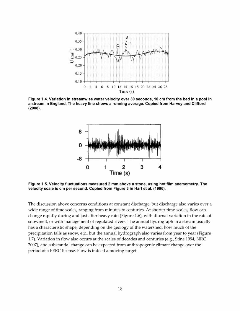
Figure 1.4. Variation in streamwise water velocity over 30 seconds, 10 cm from the bed in a pool in a stream in England. The heavy line shows a running average. Copied from Harvey and Clifford (2008).

Figure 1.5. Velocity fluctuations measured 2 mm above a stone, using hot film anemometry. The velocity scale is cm per second. Copied from Figure 3 in Hart et al. (1996).

The discussion above concerns conditions at constant discharge, but discharge also varies over a wide range of time scales, ranging from minutes to centuries. At shorter time‐scales, flow can change rapidly during and just after heavy rain (Figure 1.6), with diurnal variation in the rate of snowmelt, or with management of regulated rivers. The annual hydrograph in a stream usually has a characteristic shape, depending on the geology of the watershed, how much of the precipitation falls as snow, etc., but the annual hydrograph also varies from year to year (Figure 1.7). Variation in flow also occurs at the scales of decades and centuries (e.g., Stine 1994, NRC 2007), and substantial change can be expected from anthropogenic climate change over the period of a FERC license. Flow is indeed a moving target.

18

Days in April, 2010

3 4 5 6 7 8 9

Cha

nge

in D

isch

arge

cfs

per

min

ute

-2

-1

0

1

2

3

4

Figure 1.6. Rapid change in flow in the Big Sur River during and after a spring spate on April 4, 2010. The discharge before the spate was 170 cfs, and the peak discharge was 679 cf. Daily averaged flow, the statistic usually reported, conceals considerable variation. Data from USGS gage 11143000.

Day of the Water Year (10/1 to 9/30)

0 50 100 150 200 250 300 350

100

1000

10000

Figure 1.7. Annual variation in daily flow in Butte Creek, California, for water years 2000 to 2009 (dotted lines), plus mean (solid line). Even averaged over ten years, the annual hydrograph is not smoothed.

1.3.4. Flow and fish Fish are not randomly distributed in streams; rather, they tend to select particular positions in the stream, often in response to patterns in the flow field or cover. Drift‐feeding fish tend to hold in slow water adjacent to more rapidly moving water, as depicted in Figure 1.8. Whiting and Dietrich’s data (Figure 1.2) show that such situations can exist even when there are no boulders or large wood in the channel. The ways that fish respond to and exploit velocity gradients and turbulence in flow is described in detail in an excellent recent review (Liao 2007) that focuses on laboratory studies (e.g., Figure 1.9), but places them in a context established by field studies.

19

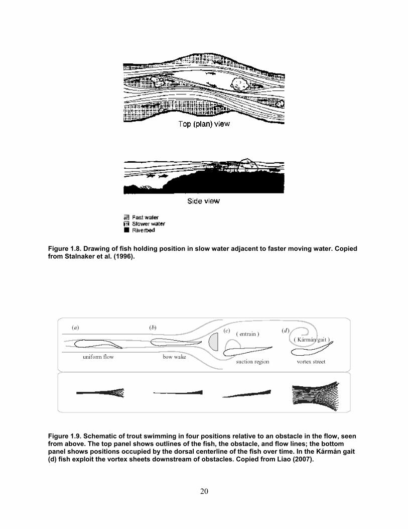
Figure 1.8. Drawing of fish holding position in slow water adjacent to faster moving water. Copied from Stalnaker et al. (1996).

Figure 1.9. Schematic of trout swimming in four positions relative to an obstacle in the flow, seen from above. The top panel shows outlines of the fish, the obstacle, and flow lines; the bottom panel shows positions occupied by the dorsal centerline of the fish over time. In the Kármán gait (d) fish exploit the vortex sheets downstream of obstacles. Copied from Liao (2007).

20

Bachman (1984:9) described another situation in which fish exploit the fine scale features of the velocity fields:

Typically, foraging sites were in front of submerged rocks or on top of but on the downward‐sloping rear surface of a rock. From there the fish had an unobstructed view of oncoming drift. While a wild brown trout Salmo trutta was in such a site, its tail beat frequency was minimal, indicating that little effort was required to maintain a stationary position even though the current only millimeters overhead was as high as 60–70 cm/s. Most brown trout could be found in one of several such sites day after day, and it was not uncommon to find a fish using many of the same sites for three consecutive years.

By holding in such positions, the fish can minimize the amount of energy that it expends per unit of energy gained by feed. Juvenile Atlantic salmon achieve much the same benefit by using their large pectoral fins to brace themselves against the stream substrate (Armstrong 2010).

Figure 1.10. Brown trout holding in the lee of a submerged stone in Spruce Creek, Pennsylvania. Copied from Figure 10 in Bachman (1984).

For fish that are holding position up in the water column in more homogenous flow, the net energy gained at a given water velocity can be modeled as benefit less cost (e.g., Figure 1.11), with both measured in units of energy per time. This is the usual biological rationale for EFMs such as PHABSIM. However, although bioenergetic modeling does show a clear peak in a plot of energy gained, the change in the energetic cost of swimming with increases in velocity appears to be small (Figure 1.12). The calculated benefit depends strongly on the ability of fish to capture drift prey, which declines when velocity increases above some threshold, and Hill and Grossman (1993) got better predictions of focal point velocity from a model based on capture efficiency than on one based on bioenergetic modeling.

21

Figure 1.11. Conceptual model for the energetic benefit from drift feeding, as a function of water velocity. Copied from Hill and Grossman (1993). Capture efficiency declines as velocity increases about some threshold, reducing the benefit.

Figure 1.12. The benefit or cost of drift feeding by small (53-70 mm SL) rainbow trout as a function of velocity, in units of cm·s-1, modeled by Hill and Grossman (1993). Parameters for the estimate of benefit were developed from feeding experiments. In summary, flow velocity is an important factor affecting the positions in streams selected by fish, as has long been recognized. However, velocity is far from the only factor, as noted by Liao (2007:1998‐1999):

22

There is a robust correlation between fish size and the scale of turbulence with which they prefer to associate (Shirvell and Dungey 1983, Webb 1998, Liao et al. 2003b). However, it has also been shown that fish inhabit turbulent flows for reasons other than hydrodynamic benefits. Size‐dependant sorting of fishes may also be determined by intraspecific competition, a factor which has been documented to play an important role in group behavior for salmonids (Heggenes 2002). Complex physical structures, such as submerged tree branches, provide three‐dimensional cover, shade and visual isolation from other fish, which reduce territorial needs (Fausch and White 1981, Doloff 1986, McMahon and Gordon 1989, Fausch 1993, Imre et al. 2002, Smith 2003). These factors may be more important than hydrodynamic‐related energy savings, since it allows individuals to avoid antagonistic intra and interspecific interactions. Increasing the structural complexity in natural streams leads to an increase in population density (Moore and Gregory 1988), with dominant fish establishing territories that presumably contain the most favorable combination of these variables (Puckett and Dill 1984).

Visual isolation from other fish is just one of the several potential factors influencing why fish choose to position themselves in habitats where turbulent flows are common. Physiological state, such as hunger, may motivate the choice to hold station in turbulent flows. Fish are attracted to microhabitats where steep flow velocity gradients exist. This is because fish can swim in the slower flow to minimize energy expenditure while maximizing food intake by foraging on disoriented prey in the faster current nearby (Jenkins 1969, Everest and Chapman 1972, Fausch and White 1981, Fausch 1984, Puckett and Dill 1984, Hayes and Jowett 1994, McLaughlin and Noakes 1998, Heggenes 2002). High turbulence levels can increase the number of predator– prey encounters and thus increase foraging efficiency (MacKenzie and Kiorboe 1995, Lewis and Pedley 2001). This may explain why starved fish prefer more turbulent currents and fish increasingly seek out turbulent flows as they become hungry (Pavlov et al. 2000). At higher levels of turbulence, a trade‐off may develop whereby more frequent prey encounters are offset by greater difficulty in capturing prey. The upper limit of turbulence, then, could be set by the destabilization ‘threshold’ of a foraging fish. This limit can be affected by other physical aspects of the environment, such as illumination levels discussed earlier. Wild fishes preferentially forage in turbulence zones under high illumination (Pavlov et al. 2000). Laboratory results confirm these observations: in the light fish hold position in a vortex street and will leave temporarily to feed, while in the dark fish choose to hold station in less complex flows and make no feeding attempts (Liao et al. 2003b, Liao 2006).

23

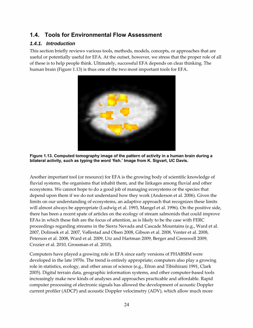
1.4. Tools for Environmental Flow Assessment 1.4.1. Introduction This section briefly reviews various tools, methods, models, concepts, or approaches that are useful or potentially useful for EFA. At the outset, however, we stress that the proper role of all of these is to help people think. Ultimately, successful EFA depends on clear thinking. The human brain (Figure 1.13) is thus one of the two most important tools for EFA.

Figure 1.13. Computed tomography image of the pattern of activity in a human brain during a bilateral activity, such as typing the word ‘fish.’ Image from K. Sigvart, UC Davis.

Another important tool (or resource) for EFA is the growing body of scientific knowledge of fluvial systems, the organisms that inhabit them, and the linkages among fluvial and other ecosystems. We cannot hope to do a good job of managing ecosystems or the species that depend upon them if we do not understand how they work (Anderson et al. 2006). Given the limits on our understanding of ecosystems, an adaptive approach that recognizes these limits will almost always be appropriate (Ludwig et al. 1993, Mangel et al. 1996). On the positive side, there has been a recent spate of articles on the ecology of stream salmonids that could improve EFAs in which these fish are the focus of attention, as is likely to be the case with FERC proceedings regarding streams in the Sierra Nevada and Cascade Mountains (e.g., Ward et al. 2007, Dolinsek et al. 2007, Vøllestad and Olsen 2008, Gibson et al. 2008, Venter et al. 2008, Peterson et al. 2008, Ward et al. 2009, Utz and Hartman 2009, Berger and Gresswell 2009, Crozier et al. 2010, Grossman et al. 2010).

Computers have played a growing role in EFA since early versions of PHABSIM were developed in the late 1970s. The trend is entirely appropriate; computers also play a growing role in statistics, ecology, and other areas of science (e.g., Efron and Tibishirani 1991, Clark 2005). Digital terrain data, geographic information systems, and other computer‐based tools increasingly make new kinds of analyses and approaches practicable and affordable. Rapid computer processing of electronic signals has allowed the development of acoustic Doppler current profiler (ADCP) and acoustic Doppler velocimetry (ADV), which allow much more

24

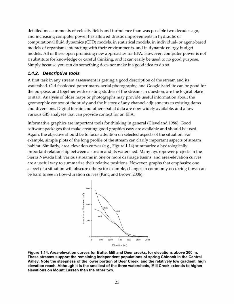
detailed measurements of velocity fields and turbulence than was possible two decades ago, and increasing computer power has allowed drastic improvements in hydraulic or computational fluid dynamics (CFD) models, in statistical models, in individual‐ or agent‐based models of organisms interacting with their environments, and in dynamic energy budget models. All of these open promising new approaches for EFA. However, computer power is not a substitute for knowledge or careful thinking, and it can easily be used to no good purpose. Simply because you can do something does not make it a good idea to do so.

1.4.2. Descriptive tools A first task in any stream assessment is getting a good description of the stream and its watershed. Old fashioned paper maps, aerial photography, and Google Satellite can be good for the purpose, and together with existing studies of the streams in question, are the logical place to start. Analysis of older maps or photographs may provide useful information about the geomorphic context of the study and the history of any channel adjustments to existing dams and diversions. Digital terrain and other spatial data are now widely available, and allow various GIS analyses that can provide context for an EFA.

Informative graphics are important tools for thinking in general (Cleveland 1986). Good software packages that make creating good graphics easy are available and should be used. Again, the objective should be to focus attention on selected aspects of the situation. For example, simple plots of the long profile of the stream can clarify important aspects of stream habitat. Similarly, area‐elevation curves (e.g., Figure 1.14) summarize a hydrologically important relationship between a stream and its watershed. Many hydropower projects in the Sierra Nevada link various streams in one or more drainage basins, and area‐elevation curves are a useful way to summarize their relative positions. However, graphs that emphasize one aspect of a situation will obscure others; for example, changes in commonly occurring flows can be hard to see in flow‐duration curves (King and Brown 2006).

Elevation (m)

0 500 1000 1500 2000 2500 3000

Are

a A

bove

Ele

vatio

n (k

m2 )

0

200

400

600

Mill

Butte Deer

Figure 1.14. Area-elevation curves for Butte, Mill and Deer creeks, for elevations above 200 m. These streams support the remaining independent populations of spring Chinook in the Central Valley. Note the steepness of the lower portion of Deer Creek, and the relatively low gradient, high elevation reach. Although it is the smallest of the three watersheds, Mill Creek extends to higher elevations on Mount Lassen than the other two.

25

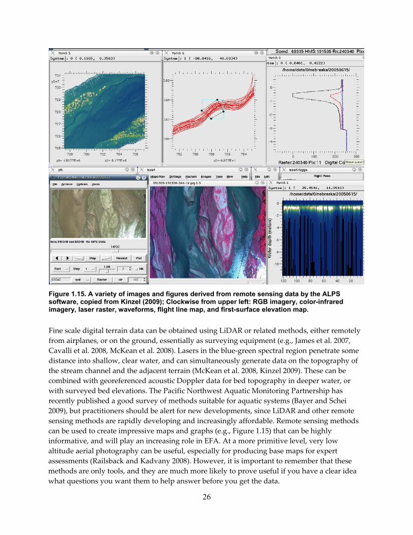
Figure 1.15. A variety of images and figures derived from remote sensing data by the ALPS software, copied from Kinzel (2009); Clockwise from upper left: RGB imagery, color-infrared imagery, laser raster, waveforms, flight line map, and first-surface elevation map. Fine scale digital terrain data can be obtained using LiDAR or related methods, either remotely from airplanes, or on the ground, essentially as surveying equipment (e.g., James et al. 2007, Cavalli et al. 2008, McKean et al. 2008). Lasers in the blue‐green spectral region penetrate some distance into shallow, clear water, and can simultaneously generate data on the topography of the stream channel and the adjacent terrain (McKean et al. 2008, Kinzel 2009). These can be combined with georeferenced acoustic Doppler data for bed topography in deeper water, or with surveyed bed elevations. The Pacific Northwest Aquatic Monitoring Partnership has recently published a good survey of methods suitable for aquatic systems (Bayer and Schei 2009), but practitioners should be alert for new developments, since LiDAR and other remote sensing methods are rapidly developing and increasingly affordable. Remote sensing methods can be used to create impressive maps and graphs (e.g., Figure 1.15) that can be highly informative, and will play an increasing role in EFA. At a more primitive level, very low altitude aerial photography can be useful, especially for producing base maps for expert assessments (Railsback and Kadvany 2008). However, it is important to remember that these methods are only tools, and they are much more likely to prove useful if you have a clear idea what questions you want them to help answer before you get the data.

26

1.4.3. Stream classifications Streams differ, and people use various categories or classification systems for thinking about them. We could not think or communicate very well without such categories. Classifications of streams can be developed in various ways, based on anything from what lives there (e.g., trout streams) to the underlying substrate (e.g., bedrock and alluvial streams) to complicated numerical analyses using principal components analysis and clustering algorithms on stream gage data (e.g., Olden and Poff 2003). It is not obvious which approach is best; the real test is how well the classification works for its intended purpose. Naiman (1998) and Montgomery and Buffington (1998) review various approaches to classification.

Classification is especially attractive for efforts to define environmental flows, or guideless for setting environmental flows, for regional groups of streams. For example, the ELOHA [ecological limits of hydrologic alteration] approach is built on identifying types of streams for which guidance can be developed (Poff et al. 2010). Similarly, R2 Resource Consultants (2004) classified sub‐basins in the Snake River drainage to develop recommendations for environmental flows for a basin‐wide stream adjudication process in Idaho. This approach seems appropriate. For thinking about environmental flows in a number of streams, it is natural to weigh experience in similar streams more heavily than experience in dissimilar streams.

However, it is important to keep in mind that the categories in stream classifications are human inventions, and not manifestations of some underlying natural order. For example, streams draining the Sierra Nevada and Cascade Mountains are can be classified as spring‐fed, rainfall‐runoff, and snowmelt runoff, but the hydrographs from these streams show a gradient across these idealized types (Appendix A of Williams 2006). Nothing about streams will generate categories as distinct as biological species, or hierarchical systems as “real” as phylogenetic trees. It is easy to forget this. For example, according to Poff et al. (2010:150): “By classifying rivers according to ecologically meaningful streamflow characteristics (citations omitted), groups of similar rivers can be identified, such that within a grouping or type of river there is a range of hydrologic and ecological variation that can be considered the natural variability for that type.” This language seems to treat types as real things, with a natural variability, rather than a conceptual convenience.

This is a practical concern. Experience with the use (or misuse) of stream classification in stream restoration work shows that real problems can result from careless use of classification systems, especially the Rosgen (1994) system (Smith and Prestegaard 2005, Kondolf 2006, Simon et al. 2007, Elliott and Capesius 2009, Miller and Kochel 2010). There seems to be a human tendency to treat the types as normative, as if the attributes of streams in a given category ought to be typical for the category, or there were something somehow wrong with a stream that does not fit neatly into the classification system.

Alternatively, stream classifications may be useful for directly assessing the effects of changes in flow on fish. Peterson et al. (2009) found that statistical models based on channel characteristics and discharge fit data on fish presence or abundance as well as models based on habitat characteristics. That is, they found they could by‐pass the usual process of predicting changes in habitat characteristics from changes in discharge. However, the utility of this approach may

27

depend on strong contrasts in the geology of the study area. See Downes (2010) for cautions about this approach.

1.4.4. Habitat classifications The discussion above of stream classifications also applies to classification of habitat types (riffles, pools, etc.); these constructs are probably essential and certainly useful for talking about streams, but they are to some degree arbitrary. Calling the types “physical biotopes” (Padmore 1998, Harvey and Clifford 2009) does not make them any more “real” (Clifford et al. 2006). The boundary between habitat types often shifts with discharge, and the contrast between pools and riffles in flow metrics such as velocity or Froude Number tends to decrease as discharge increases.

The habitat classification system described by Hawkins et al. (1993) has been popular, especially in the West, but many others have been used as well. As with stream classifications, systems of habitat types should be assessed in terms of their utility for the task at hand, and the system of types that is optimal for any given task may vary regionally, with regional variations in geology, vegetation, flow regimes or fish fauna (Williams et al. 2004). There is often an argument for applying the classification systems widely, so that data from different areas may be more easily compared, but this risks applying the systems where they do not work well. There may be no good resolution to this dilemma. Like channel types, habitat types have also been used to predict the presence and abundance of fish (Rosenfield 2003); MesoHABSIM, reviewed in section 1.5, is a method based on abundance‐environment relations developed at the spatial scale of habitat types, sometimes called mesohabitats.

1.4.5. Thought experiments IFD and IDD: Thought experiments, which can also be called qualitative or conceptual models, sometimes can shed light on complicated problems. The notions of the Ideal Free Distribution (IFD) and the Ideal Despotic Distribution (IDD), developed by Fretwell (1972), are a good example. Fretwell defined the basic suitability of a patch of habitat as the expected fitness of an organism inhabiting the patch at very low population density, and assumed that the actual suitability of the patch would decline as the local population density increased. He then considered how organisms would distribute themselves if they could accurately judge the actual suitability of habitat patches and occupy the most suitable habitat available to them. In the case of the IFD, organisms are free to occupy any patch. In this case, the population density will vary with the basic suitability of the habitat patches, but the fitness of all organisms will be approximately equal. In the IDD, on the other hand, dominant organisms exclude others from the most suitable patches, so population density does not reflect the intrinsic basic of habitat patches, and the fitness of members of the population will vary over patches.

Real organisms are unable to judge the suitability of available habitats with perfect accuracy, and will be more or less able to exclude others, so the ideal free and ideal despotic distributions are idealized end‐members of a continuum, and real distributions of organisms will fall somewhere between them. Moreover, habitats change over time, so the distributions of habitat quality will also change. Nevertheless, this simple thought experiment has been highly influential in ecology (Guillermo and Healy 1999, Gibson et al. 2008, and Imre et al. 2010 are

28

examples regarding fish), and has important implications for EFMs that try to estimate habitat quality in terms of observed population density.

Optimal habitat ratios: Generally, the productivity of stream habitats for prey species will vary spatially, as will that for predatory species, and the distributions of productivity for the two will differ, especially if prey drift in the flowing water, and so are transported from one habitat patch to others. This raises the question whether there is an optimal ratio for the two kinds of habitat. A thought experiment described in Rosenfeld and Raeburn (2009) helps clarify this question. The article also describes and discusses an actual experiment involving juvenile coho salmon in an artificial stream.

Juvenile coho are normally found in pools, and eat aquatic invertebrates that mostly rear in riffles, but often drift downstream (juvenile coho also eat terrestrial insects, but if the supply of these is roughly constant along the stream they can be ignored in the thought experiment). Starting from the upstream end of a riffle, the density of aquatic invertebrates in the drift will tend to increase downstream, but at declining rate, for a distance equal to the average drifting length for the invertebrates in question. In the pool, the density of invertebrates will decrease downstream, as they are filtered from the drift by the fish. Given that fish abundance is limited by food, there should be some spacing of riffles and pools that is optimal for the juvenile coho.

For more complex and realistic situations, for example when there are smaller fish in riffles and larger fish in pools, or there is one species in the riffles and another in the pools, the situation gets too complex to think about without a simulation model. However, the insight remains that the ratio of habitat for invertebrates and for fish matters, and the ratio can be expected to change with flow. Better tools for dealing with this issue in EFA would be helpful, as would better data.

Percent habitat saturation (PHS): For drift‐feeding fish that defend feeding territories, a thought experiment suggests that there is some population density below which fish can find suitable territories without too much conflict, and above which they cannot. Since the size of the territories will increase with the size of the fish, that population density will depend on the size distribution of the population. Grant and Kramer (1990) proposed that percent habitat saturation (PHS) is a useful statistic for assessing whether populations of juvenile salmonids are limited by the area of rearing habitat, with a critical value of about 27%, based on data from the literature. As calculated, PHS is really a length‐weighted measure of density. It may need adjustment for food supply and habitat complexity, which affect territory size, and does not apply where fish are not territorial, but PHS seems like a reasonable rule of thumb for estimating if physical habitat or some other factor is likely to limit abundance in many situations.

1.4.6. Professional opinion Professional opinion inevitably plays a large role in EFA, whether it is expressed in the selection and implementation of models or the analytical methods that are used, or more directly in subjective assessments of the likely response of stream ecosystems to management actions, for example in the Demonstration Flow Assessment approach reviewed in section 1.5. In either

29

case, it is important that the reasoning behind the judgments be documented, so that the judgments can be reviewed in light of new information. There is a growing literature on the use of professional opinion in assessments generally, as well as in Bayesian approaches, briefly reviewed in Appendix A in Hart and Polino (2009). The journal Reliability Engineering and System Safety had a special issue on expert judgment in 2008, summarized by Cooke (2008:656), who observed that “The state of the art is that expert judgment methods have crossed the threshold of scientific acceptance, but have not yet reached standardization.”

1.4.7. Statistics and modeling Statistics and modeling are potentially important tools for EFA, just as they are for other areas in applied ecology, but except for temperature models and habitat association models (HAMs) such as PHABSIM, they are not much used, particularly in FERC proceedings in California (see Section 2.0). The probable reason for the general under‐use of models in EFA is the natural tendency of managers and stakeholders to want to use established methods to get answers. Unfortunately, although models such as PHABSIM are well established, in the sense of being commonly used and accepted by agencies, there are good reasons to think that they should not be, as discussed below and in section 1.5.

Statistics can be considered the science of getting information out of data. Efron and Tibshirani (1993) remarked that “Statistics is a subject of amazingly many uses and surprisingly few effective practitioners.” This is still true, especially for environmental flow assessment, which has lagged behind other fields of applied ecology in this respect (Ahmadi‐Nedushan et al. 2006, Williams 2010a, Downes 2010).

Sampling

Sampling theory is a well developed part of statistics (e.g., Thompson 2002). Although sampling is common in EFMs, random or probability sampling is seldom applied (Williams 2010b). Curiously, decision‐makers who would give scant attention to opinion polls that were not based on probability sampling seem unperturbed by such sampling for EFMs. Purposive selection of “representative samples” is a curious departure from normal scientific practice that is not uncommon in studies of streams (Downes 2010, Williams 2010b), but should be. Information about the stream should be used for developing the sampling plan, not for selecting the sample. Probability sampling does not just avoid deliberate bias. Estimates from probability samples generally are more accurate than estimates from deliberate samples, and valid estimates of sampling error can only be calculated from probability samples. Even if all parties in a dispute over the allocation of water agree that a set of deliberately selected samples is representative of the stream in question, that does not make it so. Regarding the “representative reach” approach, Stevens et al. (2007:12) noted that:

One problematic issue is that a site representative of one variable is not necessarily representative of any other variable; another is that if the sites truly are representative of central tendency, then the extremes are suppressed. A major weakness of this technique is that humans fare poorly when integrating new data due to the existence of prior conceptions; this theory is supported by many experiments in cognitive psychology.”

30

Stevens et al. (2007) also describe a method for selecting spatially balanced probability samples, called GRTS, which seems well suited for EFMs. Software for using GRTS is available on the web (Google “GRTS sampling”). Williams (2010b) provides guidance for using probability sampling in EFMs, and describes the evidence that persuaded statisticians eighty years ago that probability sampling works better than deliberately selecting representative samples.

Resampling algorithms and statistical modeling

Computers now allow the use of statistical approaches that use resampling algorithms such as bootstrapping (Davison and Hinkley 1997, Shalizi 2010), Monte Carlo analyses (Manly 1997), or hierarchical statistical modeling (Clark 2005, Cressie et al. 2009, Ebersole et al. 2009). The bootstrap can be used to estimate confidence intervals for complex statistics such as the parameters of AERs (abundance‐environment relationship; Williams 2010a), and can also be used in various kinds of simulations. Wilcock et al. (2009) describe a Monte Carlo method for estimating the uncertainty in the critical discharge for sediment transport or the cumulative transport of sediment, given assumptions about the uncertainty in parameters such as Manning’s n or the critical Shields Number for the site. Estimating uncertainty in key parameters and calculating confidence intervals for statistics should be standard practice in EFMs.

Public domain software packages such as R and winBUGS now make the computational part of statistical analyses easy, but few people working on environmental flow assessment know how to make full use of them. For an exception, Webb et al. (2010) used Bayesian hierarchical modeling to assess the effects of modified flow regimes on salinity in two rivers in Australia, and on a species of smelt on another. They noted in their summary that

Inferring the effects of environmental flows is difficult with standard statistical approaches because flow‐delivery programs are characterized by weak experimental design, and monitoring programs often have insufficient replication to detect ecologically significant effects. Bayesian hierarchical approaches may be more suited to the task, as they are more flexible, and allow data from multiple non‐replicate sampling units (e.g., rivers) to be combined, increasing inferential strength.

Bayesian hierarchical modeling is a powerful analytical approach that is well suited for ecological problems (Clark 2005, Cressie et al. 2009). Computational requirements limited the use of Bayesian methods until recently (Ellison 1996), but computers continue to improve and appropriate software is now readily available. McCarthy (2007) provides an accessible introduction Bayesian modeling in ecology that introduces winBUGS and provides code for example problems. Grantham (2010) used hierarchical modeling with winBUGS to show that the survival of juvenile steelhead in a tributary to the Russian River varied directly with summer flow. However, like other powerful tools, winBUGS should be approached with due caution, and with guidance from someone with a firm grounding in statistics. The power of the method comes largely from a resampling algorithm, called BUGS (Bayesian using Gibbs sampling). Clarke (2007:456) observed that “Experience tells me that turning non‐statisticians loose on BUGS is like giving guns to children.” Of course, convenient statistical packages for

31

conventional frequentist statistics have been widely misused as well, so the problem of misuse is not confined to Bayesian methods. The field of EFA badly needs some good statisticians.

Modeling is too big a topic to cover in a brief review. The term describes a range of activities that can be categorized in various ways. For example, Hilborn and Mangel (1997), with an emphasis on ecological modeling, distinguished deterministic and stochastic models, statistical and scientific models, static and dynamic models, quantitative and qualitative models, and models used for understanding, prediction, and decision. Here we discuss only a few points that seem particularly relevant for EFA.

Abundance-environment relations (AERs)

Environment‐abundance relations are models that show the relationship between environmental variables such as depth or velocity and the local abundance of organisms, for example the habitat suitability criteria used in PHABSIM. Most are fit to data although some are based on expert opinion. Some are more attractive from a statistical point of view than others, as discussed below and in Appendix B. However, the inferences that can be drawn from AERs are limited. In particular, it cannot be assumed that the quality of habitats can be inferred from which habitats patches are occupied by the organism of interest. This seems a common‐sense assumption, but reasons that it may not hold have long been known (e.g., Fretwell 1972, Van Horne 1983, Power et al. 1998). Implicitly, the approach assumes that the distribution of the animals follows the Ideal Free Distribution, discussed above, but many fish are territorial, so subordinate fish may not occupy the habitat that they would select if they could. Fish may avoid otherwise favorable habitat because of predators or competitors. Fish may be selecting habitat based on environmental features at a different spatial scale from those measured, or at several spatial scales simultaneously. In any case, the habitats that are occupied and unoccupied will depend on the abundance of fish. Moreover, habitat selection can be highly variable (Vilizzi et al. 2004), and besides predators and abundance can depend on such factors as water temperature (Hill and Grossman 1993), abundance of food (Rosenfeld et al. 2005), population density (Bult et al. 1998); habitat type (Modde and Hardy 1992); time of day (Bradford and Higgins 2001), and whether the fish is resting or feeding. For use in habitat assessment models such as PHABSIM, it is generally assumed that habitat selection will be independent of discharge, but observations, simulations and experiments contradict this (e.g., Vondracek and Longanecker 1993, Shirvell 1994, Campbell 1998, Holm et al. 2001, Heggenes 2002, Railsback et al. 2003). Finally, it is usually assumed that managing flows to provide more habitats with features associated with greater local abundance will lead to increased populations, but the evidence for this is surprisingly slim, at least for habitat estimated by PHABSIM (Appendix A). Populations are determined by the rates of births, deaths, and net migration, which may well be determined by other factors. Lancaster and Downes (2010a, 2010b) give a thorough analysis of the shortcomings of inferences often drawn from AERs and a blistering response to a comment defending them (Lamouroux et al. 2010).

Resource selection functions are AERs with the property that the value taken by the function is proportional to the probability that the habitat in question will be occupied, given various assumptions described by Manly et al. (2002) and the cautions in Johnson et al. (2006).

32

Appendix B describes resource selection functions at more length. There is an enormous literature on resource selection functions or indices of habitat, mainly regarding wildlife, and for reasons that are unclear the level of statistical sophistication is generally much higher in the wildlife literature than in the freshwater fisheries literature. The same is true about testing habitat models.

Most AERs concern the central tendency in the relationships between environmental variables and species or life stage of interest. An alternative called quantile regression (Cade and Noon 2003, Konrad et al. 2008) may be more useful (Figure 1.16). As noted by Lancaster and Downs (2010: 389): “Given that organisms typically have wide tolerances and may not behave optimally with respect to the gradient at hand, it follows logically that AERs should be modeled as limiting responses.” This approach deserves more attention in EFA.

Figure 1.16. Local density of (a) baetid and (b) heptageniid mayflies across the stream bed in relation to near-bed velocity. Data were analyzed statistically as limiting relationship using quantile regression; model lines indicate the 90th and 10th quantiles (upper and lower lines, respectively. Figure and legend copied from Lancaster and Downes (2010).

Habitat association models (HAMs): Habitat association models relate the observed presence or abundance of fish or other organisms to habitat variables at the spatial scale of patches, estimate the distribution of these patch‐scale habitat features over larger areas, and use these to estimate the expected abundance of the organisms over the larger areas (Lancaster and Downes 2010). For example, PHABSIM combines hydraulic models that estimate the amount of area with given values of microhabitat variables such as depth, velocity, etc., with AERs reflecting the observed association of the fish or invertebrate in question with the microhabitat variables. Such models are reviewed in section 1.5, as are models that estimate the fitness of fish occupying a particular patch of habitat.

33

Capability models: Models that directly estimate the abundance or biomass of fish or invertebrates as a function of habitat are sometimes called capability models (e.g., Korman et al. 1994), in contrast to suitability models such as PHABSIM. Interest in the use of such models for stream management rose with availability of computers but then declined when it became clear that models fit to data on one or a few streams gave poor predictions on others, and especially on streams in different regions (Fausch et al. 1988, Korman et al. 1994). However, overfitting (using models with too many parameters) probably accounted for much of this problem, and hierarchical modeling can account for some of the variation among streams, so this judgment may be outdated. Early expectations of directly useful predictions were also unrealistic, but if models are taken as tools for developing understanding, capability models clearly can be useful (e.g., Kiffney and Roni 2007, Ebersole et al. 2009).

Other uses of models in EFA

Models have other uses in EFA. One is to explore the logical consequences of some set of ideas about the way something works. In a good example, Railsback et al. (2003) explored the consequences of common ideas about fish behavior for habitat selection, and found that the modeled habitat preference varied with discharge. Another is to embody some such set of ideas in a model, fit the model to data, and assess the ideas in terms of the fit. This works best if the fit of several such sets of ideas are compared (Hilborn and Mangel 1997, Burnham and Anderson 2002). For example, Hill and Grossman (1993) found that a model based on capture rate fit their experimental data on velocity selection by trout better than a model based on bioenergetic considerations. Models can provide clear summaries of the empirical relations among variables, as exemplified by the various models in Elliott (1994). Models can also provide standards against which to assess data. For example, field data on the growth rate of brown trout has been compared to output from models of the growth of well fed brown trout to assess habitat conditions in streams (Nicola and Almódvar 2004, but see Jenkins et al. 1999).

More generally, the proper purpose of models is to help people think, not to provide answers. As stated by Walters (1986:45): “The value of modeling in fields like biology has not been to make precise predictions, but rather to provide clear caricatures of nature against which to test and expand experiences.” To help people think, models have to focus on selected aspects of the problem at hand, which means that other aspects will be neglected. Ignoring this can be disastrous, as exemplified by the recent economic crisis. The world of credit default swaps was built on highly sophisticated models that persuaded many intelligent people that the associated risk was negligible, but they failed to recognize that a market based on houses that people cannot pay for from their earnings is unsustainable.

Bayesian Networks (BNs)

Bayesian networks are quantitative models with graphical interfaces that resemble familiar “boxes and arrows” conceptual models. However, as implemented with available software, they also have flexible data management capabilities and algorithms to estimate the probability that some variable will be in a particular state, depending on the state of other variables linked to it through the network. Mathematically, they are directed acyclic graphs. BNs were developed in the field of artificial intelligence, particularly for diagnostic tasks (e.g., what are

34

the probabilities that a patient has one or another disease, conditional on the patient’s symptoms and history), but have found application in fields ranging from environmental assessment to criminology to medicine (Marcot et al. 2001, Steventon 2008, Pourret et al. 2008). Applications of BNs to environmental assessments have mostly concerned wildlife, but have been applied to environmental flow assessments especially in Australia (Reiman et al. 2001, Hart and Polino 2009, Shenton et al. 2010, Stewart‐Koster et al. 2010). Appendix A of Hart and Pollino (2009) provides an excellent description of BNs, including their limitations. Because the models have simple graphical representations, they have proved useful and effective in group processes, including those involving stakeholders with conflicting interests (Marcot et al. 2006, Steventon 2008). We discuss BNs at more length in section 1.6.

Bioenergetic models

Bioenergetic models can be used to assess habitat quality in terms of the costs and benefits associated with living there, expressed in terms of units of energy. They are especially well suited for drift‐feeding salmonids, which typically occupy and defend feeding stations. The models can range from simple conceptual models (e.g., Armstrong 2010) to complex individual‐based models (IBMs) in which populations of simulated fish act and grow in simulated streams according to behavioral rules specified by the modeler (Railsback and Harvey 2002, Hayes et al. 2007). Bioenergetic models have been used successfully to predict habitat selection (e.g., Gowan and Fausch 2002, Hughes et al. 2003, Hayes et al. 2007), and growth (e.g., Whitledge et al. 2010). However, it should be remembered that the energy cost of swimming is not large for fish in typical drift‐feeding situations (Fig. 1.2), so the successful use of these models to predict habitat selection may have more to do with prey interception than actual bioenergetics. Individual‐based models with bioenergetic components have been used to explore cumulative watershed effects on populations (Harvey and Railsback 2007) or the logical consequences of the behavioral rules built into the models (Railsback et al. 2003, 2005). An IBM intended for flow assessment is reviewed in section 1.5.

State-dependent life-history models and dynamic energy budget models

State‐dependent life‐history models and dynamic energy budget models are highly generalized models based in basic biology that provide frameworks for considering the effects of environmental change on the life‐history patterns and fitness of animals. State‐dependent life‐history models have been applied to various salmonids (e.g., Mangel and Satterthwaite 2008, Satterthwaite et al. 2009); development of a dynamic energy budget model linked to a population model for Chinook salmon is underway with funding by PIERS. These models are applicable to EFA because the opportunity for growth provided by the environment is an important variable. Because the models estimate fitness; they can be used to explore the likely evolutionary changes in life‐history patterns resulting from changes in a stream such as those caused by dams, as well as shorter term effects. For example, state‐dependent life‐history models have been used to consider the effects of conditions in the American and Mokelumne rivers on the relative fitness of resident and anadromous life‐histories for female steelhead (Satterthwaite et al. 2010). Although the basic models are highly generalized, and therefore “unrealistic,” their base in fundamental biology is an important strength that has been lacking

35

in EFA, and the models can be elaborated for particular streams for which appropriate data are available (e.g., Satterthwaite et al. 2010).

Flow models

Changes in the computer models used to estimate flow for EFA have been as dramatic as changes in measurements of flow. Beginning in the 1970s, 1‐D flow models, originally developed for estimating the surface elevation or stage of a river, were applied to EFA, notably in PHABSIM. These were relatively crude affairs that modeled the river as a set of cross‐sections, and distributed vertically averaged velocity across the sections by some approximation (Kondolf et al. 2000). Two‐dimensional models began to be applied in the 1990s (e.g., Leclerc et al. 1995, Ghanem et al. 1996). These estimate the cross‐stream components of the velocity as well as the downstream component, but again estimate only the vertically averaged flow. A log profile can be tacked onto the vertically averaged flow, but this is a gross simplification, as shown below, and in Figure 1.2. Three dimensional models were applied to parts of natural channels by the end of the decade (e.g., Lane et al. 1999). One‐dimensional flow models are still used in many flow assessment studies, but the trend is clearly toward 2‐D modeling, and 3‐D models can now be applied to meaningful lengths of natural channels (e.g., Shen and Diplas 2008). Lane (1998) gives a description of the physics underlying hydraulic models that should be intelligible to anyone not too put off by equations involving partial derivatives. Recent papers tend to describe the hydraulic models used as “computational fluid dynamics” (CFD) models, but this seems mainly a matter of fashion.

Shen and Diplas (2008) applied 2‐D and 3‐D models to a short reach of the Smith River, Virginia, which is used for spawning by brown trout, and compared the results. 4 As would be expected, the 2‐D model was unable to resolve eddies behind boulders (e.g., Figure 1.18) which seem to affect redd‐site selection by brown trout in this stream. In other cases, such as a salmon spawning riffle in a large river, the velocity field may be homogenous enough horizontally that a 2‐D representation is adequate. Whether this is so should be determined on a case by case basis, and will depend on the particular questions that the modeling is expected to help answer.

At the base flow shown in Figure 1.17, the boulder is not submerged, but it is at the high flow shown in Figure 1.18. In this situation, there is upstream flow in the eddy behind the boulder, and a very steep velocity gradient just above the boulder. The general shape of the velocity gradient in Figure 1.18a should apply to any isolated submerged rock of similar form. This clarifies the situation described in the quotation from Bachman (1984) at p.15‐16.

If detailed modeling is or will be made available, a relevant question is what to do with the information. The answer is not clear, but there are options. One is to use the model in a HAM; that is, to combine the flow information with an AER, such as a resource selection function, to calculate some index of habitat, which could be mapped or plotted as functions of flow. 4 MacWilliams et al. (2006) describe another good comparison of 2 and 4‐D models, at a coarser spatial scale.

36

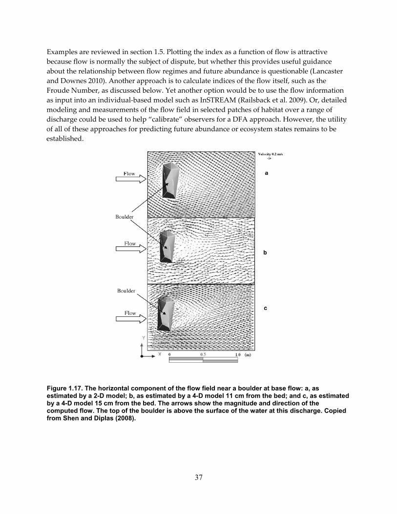
Examples are reviewed in section 1.5. Plotting the index as a function of flow is attractive because flow is normally the subject of dispute, but whether this provides useful guidance about the relationship between flow regimes and future abundance is questionable (Lancaster and Downes 2010). Another approach is to calculate indices of the flow itself, such as the Froude Number, as discussed below. Yet another option would be to use the flow information as input into an individual‐based model such as InSTREAM (Railsback et al. 2009). Or, detailed modeling and measurements of the flow field in selected patches of habitat over a range of discharge could be used to help “calibrate” observers for a DFA approach. However, the utility of all of these approaches for predicting future abundance or ecosystem states remains to be established.

Figure 1.17. The horizontal component of the flow field near a boulder at base flow: a, as estimated by a 2-D model; b, as estimated by a 4-D model 11 cm from the bed; and c, as estimated by a 4-D model 15 cm from the bed. The arrows show the magnitude and direction of the computed flow. The top of the boulder is above the surface of the water at this discharge. Copied from Shen and Diplas (2008).

37

Figure 1.18. (a) water velocity profile computed with a 4-D model for a point about 0.1 m downstream from the boulder shown in Figure 1.17, at peak flow. The point of maximum velocity is circled. The vertical lines show the mean velocities estimated by the 4-D model (0.89 m·s-1) and by the 2-D model (1.08 m·s-1). (b) As in (a), but for a point about 2 m downstream from the boulder; stars show velocity measured with ADCP equipment. Copied from Shen and Diplas (2008). Indices of hydraulic habitat

Resource selection functions or habitat suitability criteria are developed from measurements of physical characteristics of the stream at points occupied and not occupied by fish: typically depth, velocity, substrate size, and sometimes cover. As an alternative, indices can be estimated directly from measurements or model estimates of characteristics of the flow. For example, the Froude Number is a dimensionless number that has been used as an index of habitat by various authors (e.g., Lamouroux and Souchon 2002, Doyle et al. 2005, Moir et al. 2006). The Froude Number can be calculated as velocity divided by the square root of the acceleration of gravity multiplied by depth,

but this is vague unless the depth and velocity to be used are specified. Typically the number is calculated from the vertically averaged velocity and the depth at a point in a stream or across a transect (e.g., Jowett 1993), and in this case a Froude Number of one marks an important transition in the physical behavior of the flow. Alternatively, Enders et al. (2009) defined a “bed Froude Number,” using the velocity the velocity measured 10 cm above the bed, and Lamouroux and Capra (2002) calculated a Froude Number using reach‐averaged depth and velocity. The physical meaning of the number defined in these ways is unclear. Other dimensionless hydraulic variables, such as the Reynolds Number, have also been used (e.g., Lamouroux and Souchon 2002).

38

The shear stress on the streambed, or the “shear velocity,” are other potential indices of the flow field, particularly for benthic organisms. The shear stress is defined as the dynamic viscosity of the fluid times the velocity gradient, and the shear velocity is which is the square root of the shear stress divided by the density of the fluid. However, at the length scale of benthic organisms, the hydraulic environment on the bed is extremely patchy (Robertson et al. 1997), so these indices should be interpreted with caution.

Crowder and Diplas (2002) suggested using as indices the vorticity of the flow at a point, and especially the integral of the vorticity over a small area, called the circulation, which can be calculated from the output of 2‐ or 3‐D hydrodynamic models and mapped, together with flow vectors. This facilitates visualization of the structure of eddies in the flow. Although the equations defining circulation may seem daunting to most people involved in EFAs, the basic idea is not that difficult and modern methods for visualization of computed fields should help people understand how the flow field changes with discharge.

If flows are measured with velocimeters, other indices such as the “turbulent kinetic energy” (Smith et al. 2006) can be calculated from turbulent fluctuations in the flow. Because flow in natural streams is normally turbulent, the flow at a point in a stream at a given discharge has a velocity that includes downstream, cross‐stream, and vertical components, U, V, and W that can be decomposed into means and deviations from the mean:

where bars denote means and primes denote instantaneous deviations from the means, or turbulent fluctuations. Enders et al. (2009) used the standard deviation of stream‐wise velocity, turbulent kinetic energy, and shear stress (estimated as , where ρ is the density of water), as well as the bed Froude Number. Harvey and Clifford (2009) used the standard deviation and skewness of the turbulent residuals as well as turbulent intensity. Roy et al. (2010) calculated 14 indices, used a complex statistical analysis to define a smaller set of uncorrelated variables and then partition the fluctuations among six spatial scales.

It seems too soon to tell whether any of these indices will prove useful for predicting the future abundance of fish. Froude Numbers or other indices can be used to develop HSC or as independent variables in resource selection functions, but these would suffer the same problems as others. For example, Enders et al. (2009) found that juvenile Atlantic salmon tended to favor areas with low bed Froude Numbers, but variability among individuals was considerable, and may have resulted from other factors such as food supply that could override any preference for hydraulic habitat. Enders et al. (2009:1825) opined that, “Whereas Atlantic salmon parr seem to react and respond to turbulence on a smaller microhabitat scale, the application of dynamic variables on a reach scale seem to not provide a useful tool for fisheries and habitat managers.” Roy et al. (2010) concluded their abstract by noting that “Further research should attempt to link the spatial scales of turbulent flow variability to benthic organism patchiness and fish habitat use.” Even at a microhabitat scale, the relation between habitat use and any of the indices should be treated as a hypothesis. This is particularly true of relations that are detected by calculating many variables and then looking for those that best

39

match observations of fish. Statisticians call this kind of practice “data dredging,” and it is notorious for producing spurious correlations (Freedman 1993, Burnham and Anderson 1998), as discussed in Appendix A.

Hydrological indices

Since EFA is about flow, flow statistics are obvious tools to use, and the relevant question becomes, which ones? Olden and Poff (2003:111) noted that “In recent years the development and application of indices describing hydrological conditions of streams and rivers has exploded in the literature, resulting in dramatic shift from a paucity of indices in the past to the plethora of indices now available,” so the choice is not obvious. The Indicators of Hydrologic Alteration (IHA) method (Richter et al. 1996) uses 33, selected with an eye toward the effects of hydropower operations on flow, and convenient software for doing the analysis is available from the Nature Conservancy. Olden and Poff (2003) found 171 indices reported in 13 papers, generally describing the magnitude, frequency, duration, and rate of change of flow. The indices tend to be highly correlated, and Olden and Poff (2003) found that they could account for most of the variation in the indices using just a few synthetic variables defined by principal components analysis, using data from 420 gages on relatively unmodified streams. These synthetic variables are uncorrelated, which is a virtue for statistical analysis, but they do not seem to be useful aides to thinking, since they cannot be visualized. Using the IHA indices or selecting indices based on the particular questions at hand may be more useful.

Temperature models The physics of the processes that govern stream temperature are well understood, and a variety of models are available for assessing the effect of changes in discharge on temperature. Deas and Deas and Lowney (2000) provide a good review. Which models are most appropriate for any given flow assessment will depend on the resources that are available, including the time, funding, data, and modelers, and on the questions to be addressed. There is not much point to using a detailed model if appropriate input data are not available. Temperature models generally incorporate a flow model, so the possible level of detail in the temperature predictions will be limited by the flow model. Accordingly, conventional water temperature models will not be able to deal with questions about temperature variation within channels, such as thermal stratification in pools. An empirical approach probably will be more practicable in many cases.

Sediment transport models Having an estimate of the discharge needed to mobilize the bed of the stream is important for EFA for several reasons, including food chain effects (Wootton et al. 1996, Power et al. 2008), flushing fine sediment from spawning gravel (Kondolf and Wilcock 1996), and channel evolution. Sediment transport is also an inherently stochastic process that cannot be predicted in detail. Various models and equations are available for estimating sediment transport, but, as a practical matter, predicting the magnitude of coarse sediment transport is difficult and not highly accurate, largely because transport is a very steep function of the shear stress in excess of that need to initiate transport (Wilcock et al. 2009). Probably the best option for EFA is using the BAGS Excel‐based software developed for the U.S. Forest Service (Pitlick et al. 2009). This software allows sediment transport at particular sites to be modeled using several equations

40

from the professional literature. In a companion document, Wilcock et al. (2009) provide guidance for selecting appropriate equations and interpreting the output, as well as a first‐rate introduction to the topic.

41

1.5. Review of Environmental Flow Methods 1.5.1. Introduction The review of existing EFMs here is brief, because many reviews already exist (e.g., EPRI 2000, Tharme 2003, Hatfield et al. 2003, Annear et al. 2004, Acreman and Dunbar 2004). We focus on the methods that seem likely to be proposed for use in FERC proceedings, especially in the Sierra Nevada of California, such as such as the Physical Habitat Simulation System (PHABSIM). Those interested in methods used before the development of PHABSIM, or when PHABSIM seems to call for too much effort, can consult Stalnaker and Arnette (1976) or Wesche and Rechard (1980), or the recent reviews just mentioned. This review deals with EMFs as applied to fish or aquatic invertebrates, although geomorphic and riparian aspects of ecosystems should also be taken into account in flow evaluation processes.

Like most things, EMFs can be classified in various ways. A common distinction is between ‘incremental’ and ‘standard‐setting’ methods. This distinction is dubious, because flow requirements are often called flow standards, so that any EFM that is used to set flow requirements is in that sense standard‐setting. However, the intended distinction is between (a) methods that yield flow standards directly as some function of the flow regime at the site, such as X% of the median annual flow, and (b) methods that estimate habitat value or some measure of fish abundance as a continuous function of the flow, so that the benefit or cost of incremental changes in the flow regime can be assessed. Perhaps a more useful distinction is between hydrologically based methods and habitat‐based methods that average assessments of conditions in patches of habitat as a function of flow.

This section briefly reviews environmental flow methods (EFMs) distinguishing between top‐down and bottom‐up methods (discussed next), and between flow or hydrology‐based and habitat‐based methods. Habitat‐based methods generally involve sampling, which is discussed next, along with some general comments, followed by discussion of three analytical frameworks, IFIM, DRIFT, and adaptive management, within which EMFs may be implemented. The section ends with a review of other reviews of EFA or EMFs, and some conclusions.

1.5.2. Top-down and bottom-up approaches There are two ways to think about the consequences of modifying the flow regime in a stream: in terms of how much the flow regime can be modified without causing too big an effect (top‐down), or in terms of what flows are needed for various ecological purposes (bottom‐up). The “Natural Flow Paradigm” (Poff et al. 1997) provides a basis for the top‐down approach. Essentially, it calls for attention to five attributes of the flow regime: magnitude, frequency, duration, timing, and rate of change (other authors also add seasonality), and to changes in these resulting from regulation. Ecological responses to changes in these attributes from flow regulation are pervasive, but not enough data are yet available to define widely applicable quantitative relationships (Poff and Zimmerman 2010), so judgment and river or region‐specific information must be used.

42

The bottom‐up approach involves defining what needs to remain in the river, as in the common California practice of having different flow standards for salmonid spawning, rearing, migrations, etc., although holistic approaches such as the South African Building Block methodology (King et al. 2008) take a broader view. Bottom‐up methods logically require understanding what matters about the flow regime for the stream in question. In many instances, and particularly when trying to improve an already severely modified flow regime, there is no alternative to acting as if one did have such understanding (e.g., Moyle et al. 1998), although ecological uncertainty can still be taken into account through monitoring and adaptive management. Some scientists seem more confident of their understanding, for example Jowett and Biggs (2009:1127):

If the natural ecosystem is to remain unchanged in terms of both community composition and abundance, the only management option is to maintain the natural flow regime. However, in most situations it should be possible to develop a set of management goals and a flow regime that maintains the ecosystem in a state that is indistinguishable from the natural one or even improves upon some valued aspects, recognizing that in some instances this may be at the expense of less valued aspects (Beecher, 1990).

As should be clear from section 1.2, we do not think this confidence in our ability to manage streams to exactly fit our needs is warranted, unless the objective is simply to turn an unruly river into a nice trout stream.

1.5.3. Flow (hydrology) based methods Indicators of hydraulic alteration (IHA) The IHA or Range of Variation method is based on the sensible idea that flow regimes should be based not just on measures of the central tendency, but also on measures of variation (Poff et al. 1997). The method was developed by Brian Richter and colleagues with the Nature Conservancy (Richter et al. 1996, 1997, 1998), and software for the analysis is available on‐line from the Nature Conservancy. The method calculates 32 statistics on the magnitude, duration, timing, and rate of change of flow from daily time series, for both a base period, usually unimpaired or existing conditions, and the proposed conditions. The differences between the two sets of statistics provide a measure of the hydrological effects of the project, but the ecological effects remain to be assessed. Some rule of thumb about the maximum allowable change could be used, but the real strength of the approach is to direct attention to the various aspects of the flow regime that need to be considered. The available software makes calculating and graphing the statistics easy, so the main task required is to develop the input data. Even for systems with long gage records, this may be non‐trivial, since conditions in many watersheds will have changed gradually over the period of record, and reconstructing a record of unimpaired flow flows can be difficult enough on a monthly basis, if the flow is significantly affected by diversions. Reconstructing daily flows will generally require considerable estimation. Nevertheless, use of the IHA should be routine in FERC assessments, but it should be used to provide food for thought, not as a source of answers.

43

ELOHA The recently developed Ecological Limits of Hydrologic Alteration (ELOHA) approach to developing environmental flow standards has received considerable attention from scientists working in EFA (e.g., Poff et al. 2010), and is clearly related to the IHA. As described by Kendy et al. (2009), the main steps in the ELOHA approach are: “(1) build a hydrologic foundation, (2) characterize river types according to their flow regimes and geomorphic features, (3) compute present‐day degrees of flow alteration, (4) define flow alteration‐ecological response relationships, and (5) use flow alteration‐ecological response relationships to manage environmental flows through an informed social process.” Unfortunately, although the available literature does confirm that ecological responses to flow regulation are pervasive, it does not provide the data needed to define flow alteration‐response relationships (Poff and Zimmerman 2010). Although some of the concepts involved are useful for FERC processes, the method was designed for developing standards at a regional scale, especially in data sparse situations. As such, it does not seem directly applicable to FERC proceedings that deal with one or a few streams.

Generally, in FERC license proceedings, especially relicensing proceedings, the current hydrology is well known, although climate change will introduce long‐term uncertainty into future hydrology, and developing relationships between current or future hydrology and ecological responses in a stream will be more relevant than developing general relationships between flow alteration and ecological responses. Information useful for one purpose will be useful for the other, but FERC processes probably have greater potential to provide useful information for ELOHA than the other way around.

Hydraulic geometry Despite the obvious variability among and along rivers, various authors have reported that the regularities that seem to exist in hydraulic geometry can be used to advantage in EFA (e.g., Jowett 1998, Lamouroux and Jowett 2005, Rosenfeld et al. 2007, Booker 2010). Generally, these papers refer back to a classic paper (Leopold and Maddock 1953) that noted that the variation with discharge in stream width, depth, and velocity at a station could be described by simple power functions, and that the same variation at stations along a stream could be described by other simple power functions:

w = aQb, d = cQf, v = kQm

where w, d, and v are width, depth, and velocity, and Q is discharge. By continuity, since Q = width times depth times velocity, the sum b, f, and m, and the product of a, c, and k, equal 1. Jowett (1998:451) reported that “Hydraulic geometry can be used to indicate whether hydraulic conditions approach a ‘threshold’ such as a minimum acceptable depth or velocity, thus predicating the need for more extensive habitat survey and analysis.” Rosenfeld et al. (2007:765‐6) found with some qualifications that “… hydraulic geometry relationships performed reasonably well for predicting optimal flows, …” although they actually meant optimal flows as defined by PHABSIM.

44

The reported success of hydraulic geometry methods may seem strange, given the variation in most stream channels that is apparent to anyone who has walked along them, and various authors have found considerable variation in the hydraulic geometry exponents, as discussed in Hatfield et al. (2003). Recently, Fonstad and Marcus (2010) described the along‐stream variation in stream width and depth using data from aerial photography or from transects measured every 100 m over many kilometers of stream. The along‐stream variation in width is considerably greater than the along‐stream change predicted by downstream hydraulic geometry (Figure 1.21), and similar results were reported for depth. That is, the widths and depths predicted by hydraulic geometry are so highly smoothed that their practical utility for EFA is dubious.

Biased sampling may explain why predictions from hydraulic geometry seem to be useful. The data for the hydraulic geometry studies have been from transects used for rating stream gages, or from PHABSIM studies. The rating transects are deliberately selected for as regular as possible a flow field. PHABSIM transects are also almost always deliberately selected, in part to avoid complex flow fields, and it seems likely that investigators either deliberately or unconsciously select transects that seemed to them to represent the central tendency of the stream or habitat type being sampled. In addition, Jowett (1998) averaged transects over multiple study sites, further suppressing variation. In short, using simplified hydraulic geometry to determine fish‐habitat relationships is likely to lead to results that have little relationship to the real stream in which the organisms live.

Figure 1.19. Variation in width along the Nueces River, Texas, at low flow, determined from digital aerial photography by Fonstad and Marcus (2010), together with width estimated from downstream hydraulic geometry (DHG width). Copied from Figure 2 in Fonstad and Marcus (2010).

1.5.4. Habitat-based methods Habitat-abundance and numerical habitat models (HAMs and NHMs) Habitat‐abundance models estimate the distribution of patch‐scale habitat features over larger areas of the stream channel at different flows, and use these to estimate the total habitat value of the larger areas. Generally, these models combine hydraulic or CDF models with abundance‐

45

environment relations (AERs), and the term “numerical habitat model” (NHM) has also been used for them (e.g., Guay et al. 2000). As these authors define the term, NHMs are models that combine hydraulic or CDF models and biological indices to predict the suitability or habitat value of patches of stream, which they called “tiles.” Findings are developed by ʺintegrat(ing) the predilection of fish for the substrate diameter, the water depth, and the current speed in that tile (Bovee 1978, Mathur et al. 1985, Leclerc et al. 1994). The end result of the NHM is a map describing the habitat quality index assigned to each tile at a given flow rateʺ (Guay et al. 2000:2065). This can be summarized as a plot showing the average habitat index as a function of flow or, if the model results are combined with a hydrograph, a plot showing the habitat index as a function of time. Other habitat attributes such as cover are sometimes used as well as depth, velocity, and substrate. This is supposed to estimate the expected future abundance of the organisms over the larger areas (USFWS 1979, Lancaster and Downes 2010), although this last step in the process is often left implicit.

The Physical Habitat Simulation System, PHABSIM, (Bovee 1982, Bovee et al. 1998), which estimates an index called weighted usable area (WUA), is by far the best known and most widely used of these models (Souchon et al. 2008). It was developed with 1‐D hydraulic models in the late 1970s by an interagency working group. Although two‐dimensional hydraulic models are now often used, the basic approach has remained remarkably stable. Bovee et al. (1998) and Waddle (2001) describe PHABSIM and its application in detail.

PHABSIM was regarded as a major advance over earlier EFMs, and rapidly gained acceptance despite cogent early criticisms (Mathur et al. 1985, Shirvell, 1986, Scott and Shirvell 1987) that have never really been answered, and a lack of good evidence for a strong relationship between WUA and the abundance or biomass of fish (Appendix A). Of course, it can be argued that PHABSIM or other NHMs model habitat, not fish abundance or biomass, and there are many reasons why abundance or biomass might not be related to habitat in particular cases (e.g., Gore and Nestler 1988). However, as noted by Conder and Annear (1987:339), “Use of PHABSIM relies on the assumption that a positive linear relationship exists between WUA and physical habitat, with the implied assumption that a relationship exists between physical habitat and standing crop.” Certainly this was the original idea (USFWS 1979). Evidence for such a relationship is scant, as discussed in Appendix A. Moreover, most uses of PHABSIM depend not just on the existence of such a relationship under the conditions at the time of the study, but on the assumption that changes in WUA will lead to corresponding changes in abundance or biomass. As explained by Orth (1987), and recently by Lancaster and Downs (2010a, 2010b), such predictions cannot reliably be made with PHABSIM or other models based on AERs, because populations are determined by births, deaths, and net migration, which are affected by many factors besides physical habitat. Because it is so widely used, we describe and critique PHABSIM and tests of it in some detail in Appendix A. Here, we simply note that PHABSIM was rooted in two ideas that were common when it was developed: that stream ecosystems are basically equilibrium systems, and that stream ecosystems are structured primarily by abiotic factors. The thought was that the abundance of cohorts was controlled by equilibrium ecological processes and by physical habitat through density‐dependent processes, so that if a stream were “fully seeded,” the number of fish would reflect environmental conditions, making modeling

46

instream flow relationships fairly simple. Such ideas have been abandoned by contemporary ecologists (Mangel et al. 1996, Power 1990, Wipfli and Baxter 2010). Improved understanding of how stream ecosystems function therefore requires improved EFA methodologies that can incorporate dynamic physical and biological processes, as well as uncertainty.

InSTREAM InSTREAM is a complex and sophisticated individual‐based model (IBM) for stream–dwelling salmonids. As described in the abstract of Railsback et al. (2009):

InSTREAM is a simulation model designed to understand how stream and river salmonid populations respond to habitat alteration, including altered flow, temperature, and turbidity regimes and changes in channel morphology. The model represents individual fish at a daily time step, with population responses emerging from how individuals are affected by their habitat and by each other (especially via competition for food). Key individual behaviors include habitat selection (movement to the best available foraging location), feeding and growth, mortality, and spawning. Fish growth depends on prey availability and hydraulic conditions. Mortality risks due to terrestrial predators, piscivorous fish, and extreme conditions are functions of habitat and fish variables. Field and analysis techniques for applying InSTREAM are based in part on extensive analysis of the model’s sensitivities and uncertainties. The model’s software provides graphical displays to observe fish behavior, detailed output files, and a tool to automate simulation experiments.

The model’s original purpose was to address one of the most difficult general problems of impact assessment for stream‐dwelling trout: understanding how alteration of habitat affects populations of animals that actively adapt to habitat change by moving. InSTREAM can predict how trout populations respond to changes in any of the inputs that drive the model, especially flow, temperature, turbidity, and channel morphology. InSTREAM can also predict how populations respond to changes in ecological conditions such as food availability or mortality risk. Because InSTREAM provides an observable virtual ecosystem, it is also a useful tool for addressing many basic ecological research questions.

Importantly, InSTREAM models the effects of flow on the fitness of the modeled fish, not just on which microhabitats the fish should select, and so predicts the response of populations to the flow regime. As an “observable virtual ecosystem,” InSTREAM has proven valuable; for example, Railsback et al. (2003) showed that, given reasonable rules about how salmonids respond to their environment, we should expect that habitat selection will vary with discharge, contradicting a fundamental assumption of PHABSIM. Whether InSTREAM can usefully predict the effects of management on the abundance of fish in real streams is much less clear. InSTREAM is a simulation model, and as such an application of InSTREAM is a thought experiment (Schnute 2003). As complex as it is, the virtual ecosystem described in InSTREAM is enormously less complex than real ecosystems. Railsback et al. (2009) are forthcoming about these simplifications, for example, at p. 10:

47

Trout have additional adaptive behaviors that we have chosen not to represent mechanistically in this version of InSTREAM, because doing so does not seem necessary to meet the model’s purposes. These behaviors include variation in diel activity patterns (feeding vs. hiding); allocation of energy intake to growth, energy storage, or gonad production; year‐to‐year spawning effort.

Similarly, the amounts of food available in the drift and on the bottom are treated as constant in time and space. Some of the behavioral rules coded into the program, such as the rule that fish do not feed at night, are unrealistic (Bradford and Higgins 2001, Armstrong 2010). Spawning habitat is described only in terms of area. In the current version, flow is represented by a 1‐D hydraulic model. This leaves the model open to the criticism of complex models generally by May (2004:793): “It makes no sense to convey a beguiling sense of ‘reality’ with irrelevant detail, when other equally important factors can only be guessed at.” The Recovery Science Review Panel, convened by NOAA Fisheries to provide guidance for salmon recovery efforts coast‐wide, was sharply critical of the Ecosystem Diagnosis and Treatment (EDT) model, which is now widely used in Washington and Oregon, largely on that basis: “The inclusion of so much detail may create an unjustified sense of accuracy, but actually introduces sources of inaccuracy, uncertainty, and error propagation” RSRP (2000:6). Applied to particular streams, InSTREAM is probably best used as a useful source of hypotheses, rather than as the basis of a function that relates flow regime to population abundance.

MesoHABSIM MesoHABSIM (Parasiewicz 2001, 2007) is a HAM based on AERs developed at the spatial scale of habitat types, or mesohabitats, which has been used mainly in the Northeast. Development of the method was motivated at least in part by the extensive field work required by PHABSIM. Briefly summarized, the steps in MesoHABSIM are:

• Map habitat types at four or five different flows spanning the range of management interest;

• Measure abundance and habitat attributes in all habitat types in “representative” sites;

• Develop AERs relating the presence or abundance of fish to habitat attributes in the habitat types;

• Estimate the distribution of the habitat attributes in the habitat types at the different levels of discharge, accounting for changes in the boundaries of the types;

• Calculate expected abundance at the four or five flows and interpolate between them to estimate future abundance as a function of flow.

The implementation of MesoHABSIM seems more thoughtful than most implementations of PHABSIM, but still suffers problems such as the statistically unsupportable deliberate selection of sample sites. Importantly, Parasiewicz and Walker (2007) published a comparison of fish abundance with the habitat index used by MesoHABSIM, with data collected a year after the data used to develop the model. There was a statistically significant relationship (Figure 1.22), but a great deal of scatter in the data, and a hint of a bimodal response, which raises the question whether simpler indices or professional judgment might perform as well. Moreover, the data showed high variability in the number of fish collected by electroshocking at 220

48

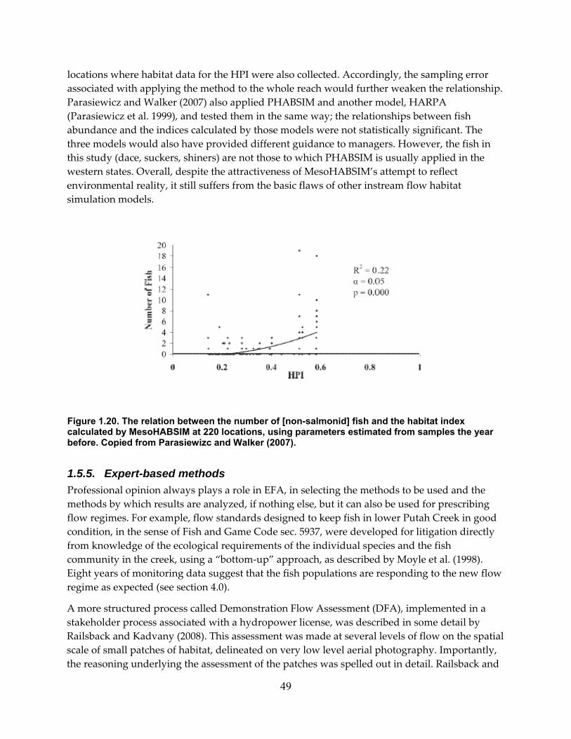
locations where habitat data for the HPI were also collected. Accordingly, the sampling error associated with applying the method to the whole reach would further weaken the relationship. Parasiewicz and Walker (2007) also applied PHABSIM and another model, HARPA (Parasiewicz et al. 1999), and tested them in the same way; the relationships between fish abundance and the indices calculated by those models were not statistically significant. The three models would also have provided different guidance to managers. However, the fish in this study (dace, suckers, shiners) are not those to which PHABSIM is usually applied in the western states. Overall, despite the attractiveness of MesoHABSIM’s attempt to reflect environmental reality, it still suffers from the basic flaws of other instream flow habitat simulation models.

Figure 1.20. The relation between the number of [non-salmonid] fish and the habitat index calculated by MesoHABSIM at 220 locations, using parameters estimated from samples the year before. Copied from Parasiewizc and Walker (2007).

1.5.5. Expert-based methods Professional opinion always plays a role in EFA, in selecting the methods to be used and the methods by which results are analyzed, if nothing else, but it can also be used for prescribing flow regimes. For example, flow standards designed to keep fish in lower Putah Creek in good condition, in the sense of Fish and Game Code sec. 5937, were developed for litigation directly from knowledge of the ecological requirements of the individual species and the fish community in the creek, using a “bottom‐up” approach, as described by Moyle et al. (1998). Eight years of monitoring data suggest that the fish populations are responding to the new flow regime as expected (see section 4.0).

A more structured process called Demonstration Flow Assessment (DFA), implemented in a stakeholder process associated with a hydropower license, was described in some detail by Railsback and Kadvany (2008). This assessment was made at several levels of flow on the spatial scale of small patches of habitat, delineated on very low level aerial photography. Importantly, the reasoning underlying the assessment of the patches was spelled out in detail. Railsback and

49

Kadvany (2008) also discuss issues related to group processes, such as ways to minimize the effects of biases or strong personalities on the assessment.

Gard (2009) described a test of DFA in the Trinity River, which found considerable variation in replicate assessments. However, in this test, the assessments were essentially just visual estimates of depth, velocity, substrate, and cover, in a large river (about 500 cfs at the time of the surveys). There may be less variation among replicate assessments of depth, velocity, and substrate in smaller streams and visual assessments are also likely to be less expensive relative to hydraulic modeling on such streams. However, to the extent that DFA is just a HAM implemented though visual assessments of standard microhabitat variables, it will share the shortcoming of other HAMS. Moreover, HAMs also suffer replication problems, as discussed below.

We find the DFA process attractive, despite the replication problems raised by Gard (2009), provided that the reasoning underlying the assessments is clearly articulated, the assessment involves more than fine‐scale microhabitat conditions, and the method is implemented in the context of adaptive management. That is, those doing the assessments should be required to articulate the assumptions and reasoning underlying their assessments, in a way that allows for developing hypotheses about the relationship between flows and habitats or populations that can be tested. Bayesian Networks should provide a useful framework for this process. Clearly, the utility of the DFA method will vary with the knowledge of the assessors, but the method makes it possible to take account of information beyond that summarized in habitat indices, such as effects over different temporal and spatial scales.

1.5.6. Sample-based methods Although hydrologically based approaches such as IHA deal with entire streams or sections of streams, most HAMs, fitness models, or DFAs deal with only samples of the length of stream to which the results will be applied. Generally, these methods assess spatially explicit patches in terms of local population density (or probability of use), or in terms of the expected fitness of fish occupying the patches (Armstrong 2010). This raises the question how well the sample of patches represents the whole length, or, stated differently, how different would the result be if the EFM had been applied to the whole length? This is a question common to many areas of human endeavor, from science to opinion polling to industrial quality control, and methods for addressing it are well worked out. These allow knowledge about the thing to be sampled to be incorporated into the sampling design, often through stratified sampling. Although it is not possible to tell how closely a given sample resembles the whole that it is supposed to represent, it is possible to quantify how close it is likely to be. That is, a probability distribution for the difference between the sample and the whole can be calculated, provided that the sample was selected randomly. Typically, the probability distribution is summarized by standard errors or confidence intervals. Sampling methods appropriate for EMFs are described in Williams (2010b), and are applicable to methods such as DFA and InSTREAM as well as PHABSIM. Not only does probability (random) sampling allow for assessing the accuracy of the results, it also gives more accurate results than deliberately selected samples, as statisticians have recognized since the seminal paper comparing the two methods by Neyman (1934).

50

Curiously, the samples for EFMs are almost always selected deliberately and results of EFMs are almost always reported without confidence intervals, despite calls that they are critical by Castleberry et al. (1996). It has also been demonstrated that with the typical number of transects used for 1‐D PHABSIM, confidence intervals are likely to be wide (Williams 1996, 2010a). Two published studies (Payne et al. 2004, Gard 2005) that challenged the results in Williams (1996) used methods that resampled a sample, like the bootstrap method used by Williams (1996, 2010a), but resampled without replacement. This treats the sample as the very population that the sample is supposed to represent, and thus underestimates sampling error when subsamples are compared. This is an elementary mistake. That these papers survived peer review illustrates the generally low level of statistical competence exhibited by practitioners of EFA (noted in section 1.4), as does the following remarkable comment on an earlier version of Williams (2010a), by a reviewer for the Transactions of the American Fisheries Society, who knows better than generations of statisticians:

It [deliberately selecting samples] comes about because the purpose of the habitat survey is to get the best estimate of the habitat index ‐ not to develop confidence intervals. It is for this reason that transect cross‐sections are rarely selected truly randomly in the inefficient fashion favored by statisticians. The main point is that random selection is the most inefficient method possible to select cross‐sections that represent hydraulic and habitat variability in the reach. This was pointed out by reviewers of his earlier paper.

Payne et al. (2004) compiled statistics on the number of transects in 616 1‐D PHABSIM studies; the mean was 10.66 (standard deviation = 9.71) and the median was 8.0. For the 572 studies that reported the length of the study reach, the mean and median number of transects per kilometer were 1.7 and 9.7, respectively. Thinking that such studies can produce reliable results verges on delusion (Figure 1.23).

51

WU

A a

t 4.2

5 m

3 s-1

20

40

60

80

100

20

40

60

80

100 n = 28n = 9

WU

A a

t 4.2

5 m

3 s-1

WU

A a

t 4.2

5 m

3 s-1

20

40

60

80

100 n = 55 Figure 1.21. Means and bootstrap 95% confidence intervals for juvenile WUA at 4.25 m3·s-1, for 50 samples of the Cache la Poudre River WUA curves, stratified by habitat type, with sample sizes of 9, 28, and 55, and no errors. These show the variation that might be expected in the results of repeated applications of PHABSIM that were perfectly accurate except for transect sampling error. The dotted lines show the overall mean for the 107 curves from which the samples were drawn. Copied from Williams (2010a).

1.5.7. Some comments on EFMs The importance of food

Most EFMs and EFAs in North America embody a rather limited and linear view of stream systems, with physical habitat as the dominant control of fish populations, as pointed out by Hatfield et al. (2003) and depicted in Figure 1.13. The importance of food and water quality gets a nod, but the analysis of physical habitat, as by PHABSIM, dominates the assessment. When invertebrates are considered, it is often through a separate PHABSIM analysis, rather than a bottom‐up ecologically oriented approach (e.g., Gore et al. 2001). However, recent studies indicate that the growth of stream salmonids, and so likely their probability of survival, responds to the available supply of food at surprisingly low population densities (Jenkins et al.

52

1999, Imre et al. 2010; Figure 1.19). Other studies have confirmed the negative power law relationship between density and growth, such that growth decreases at a declining rate as density increases (e.g., Gibson et al. 1998, Imre et al. 2010), with exploitative competition for drifting prey as a likely cause (Imre et al. 2010). Differences in site quality can also lead to such a relationship (Ward et al. 2007), especially when multiple age classes are present (Imre et al. 2010), but it seems clear that the food supply matters. Ward et al. (2009:141) concluded that “Our results suggest that an increase in prey biomass should lead to increased mean growth even if it is associated with a relatively large increase in fish population density. Clearly, salmon restoration and management efforts need to consider anthropogenic factors that influence prey abundance.” The point is elaborated by Wipfli and Baxter (2010), who argue for consideration of food from local, tributary, terrestrial, and, where anadromous fish occur, marine sources. Environmental flow assessments should pay more attention to sources of food and other aspects of food webs than has been common.

Figure 1.22. Cartoon of the conceptual model linking flow to fish that underlies most EFAs, copied from Hatfield et al. (2003). “Other impacts” and “Other ecological stuff” are acknowledged, but not really incorporated into the assessments.

53

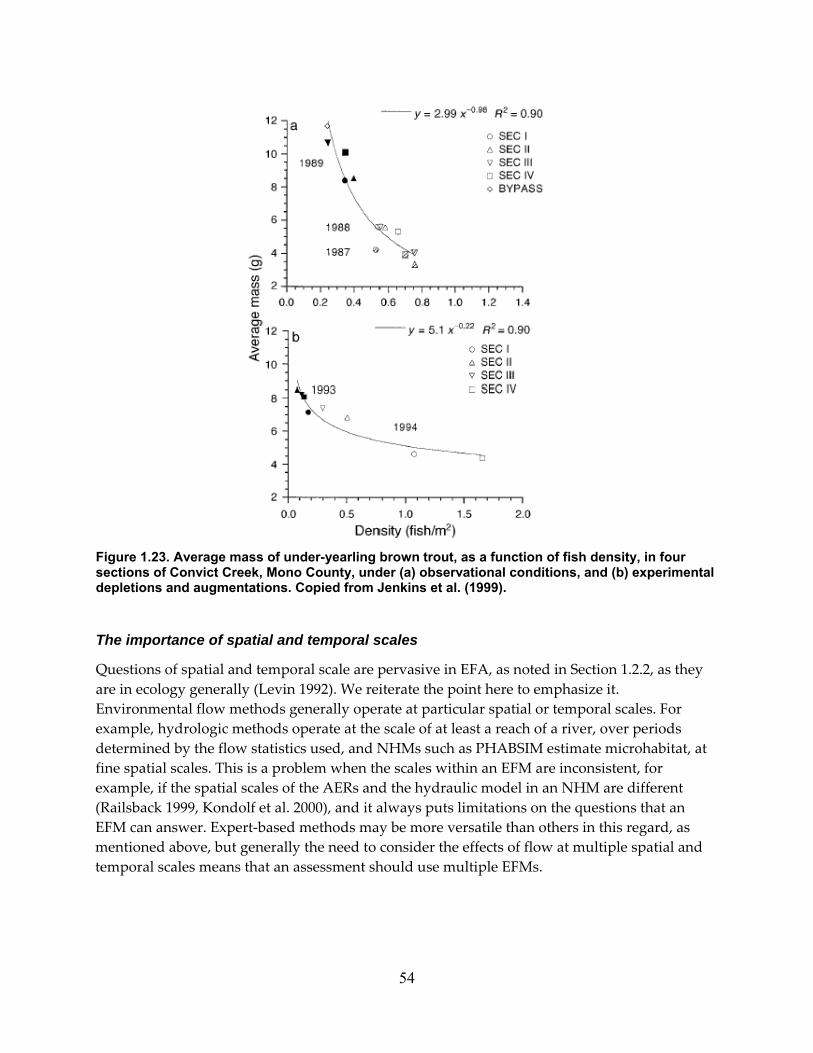
Figure 1.23. Average mass of under-yearling brown trout, as a function of fish density, in four sections of Convict Creek, Mono County, under (a) observational conditions, and (b) experimental depletions and augmentations. Copied from Jenkins et al. (1999).

The importance of spatial and temporal scales

Questions of spatial and temporal scale are pervasive in EFA, as noted in Section 1.2.2, as they are in ecology generally (Levin 1992). We reiterate the point here to emphasize it. Environmental flow methods generally operate at particular spatial or temporal scales. For example, hydrologic methods operate at the scale of at least a reach of a river, over periods determined by the flow statistics used, and NHMs such as PHABSIM estimate microhabitat, at fine spatial scales. This is a problem when the scales within an EFM are inconsistent, for example, if the spatial scales of the AERs and the hydraulic model in an NHM are different (Railsback 1999, Kondolf et al. 2000), and it always puts limitations on the questions that an EFM can answer. Expert‐based methods may be more versatile than others in this regard, as mentioned above, but generally the need to consider the effects of flow at multiple spatial and temporal scales means that an assessment should use multiple EFMs.

54

The importance of a clear purpose

Even a good EFM can address only a subset of the questions that should be considered in an assessment, as suggested above. Accordingly, assessments normally should include multiple EFMs, and those doing the assessment should be as clear as possible about which questions are important in the situation at hand before EFMs are selected. Ordinarily, however, new questions will arise during the course of the studies. This underscores the importance of an adaptive approach.

1.5.8. Frameworks for EFA Instream Flow Incremental Methodology (IFIM): The IFIM is the framework most commonly proposed for EFA in the US. The IFIM was developed by an interagency group in the late 1970s (Appendix A), largely in response to a surge in applications for small hydropower plants following the energy crisis of that decade. As described by Annear et al. (2004:187):

“The Instream Flow Incremental Methodology (IFIM) is a modular decision support system for assessing potential flow management schemes. This method quantifies the relative amounts of total available habitat available throughout a network of stream segments for selected flow regimes. It was designed to prescribe instream flow regimes that result in no net loss of total habitat, or to develop mitigation plans to compensate for habitat potentially lost as a result of proposed flow management.

…

The IFIM is composed of a library of linked analytical procedures that describe the spatial and temporal features of habitat resulting from a given river regulation alternative. The unique feature of IFIM is the simultaneous analysis of habitat variability over time and space. This methodology is composed of a suite of computer models, manuals, and data collection procedures that address hydrology, biology, sediment transport, and water quality (see Stalnaker et al. 1995 and Bovee et al. 1998). Several studies have demonstrated the relation between usable habitat and fish populations (Orth and Maughan 1982, Nehring and Miller 1987, Bovee 1988, Jowett 1993, Nehring and Anderson 1993). …

The IFIM and PHABSIM were developed simultaneously, and the terms IFIM and PHABSIM are frequently confused, in part because there is not a crisp definition of IFIM, and in part because the terminology has not been consistent over time. 5 However, Bovee et al. (1998) begin by stating:

5 This was particularly true in the 1980ʹs, when articles in the professional literature that were really about PHABSIM came out under titles such as ʺEvaluation of the instream methodology for recommending instream flows for fishʺ (Orth and Maughan 1982), or ʺA critique of the instream flow incremental methodologyʺ (Marthur et al. 1985).

55

The Instream Flow Incremental Methodology (IFIM) is a decision‐support system designed to help natural resource managers and their constituencies determine the benefits or consequences of different water management alternatives. Some people think of IFIM as a collection of computer models. This perception is understandable because IFIM is supported by an integrated habitat simulation and analysis system that was developed to assist users in applications of the methodology. However, IFIM should be considered primarily as a process for solving water resource allocation problems that include concerns for riverine habitat resources. (p. 1.)

Orth (1987, p. 171) similarly notes that ʺ(T)he IFIM process includes evaluation of effects of incremental changes in stream flow on channel structure, water quality, temperature, and availability of suitable microhabitat in order to recommend a flow regime that will maintain existing habitat conditions.ʺ However, he adds that ʺThe physical habitat component (PHABSIM; Milhous et al. 1984) is the most frequently used component, often to the exclusion of other components.ʺ Orth is not the only one to suggest that in practice IFIM usually boils down to PHABSIM: Shrivell (1986) said flatly that ʺIFIM is PHABSIM.ʺ EPRI (2001), in a review of instream flow assessments in Federal Energy Regulatory Agency processes, reports that although PHABSIM was the method most commonly used, the IFIM process was rarely implemented.

IFIM as initially proposed and as described by Bovee et al. (1998) is nevertheless worth considering, partly because it represented an attempt to take a more comprehensive approach to assessing instream flow needs, and partly because it illuminates the orientation of the developers of PHABSIM. Bovee et al. (1998) begin with a broad perspective, depicted in their first figure (Figure 1.24), showing concern for water quality and channel structure as well as microhabitat. Their third figure (Figure 1.25) draws attention to errors in observations and modeling that should be taken into account. However, it is easy to suspect that these figures were not designed for carefully consideration, since Figure 1.24 seems to depict an endless loop, the ‘observed values’ and ‘system conceptualization’ boxes on the right side of Figure 1.25 have nothing to do with the output of the real system, the ‘parameterization’ box is in the wrong place, and there should be a directed linkage from ‘system conceptualization’ box to the ‘system representation’ box.

More attention is given to negotiation. The fundamental concern permeating Bovee et al. (1998) is with successfully negotiating instream flow agreements. Much of the document (e.g., Chapter 2) concerns negotiations per se, and this emphasis caries over into the discussion of the technical aspects of the work. For example, in explaining the need to define a ʺcurrencyʺ for such a negotiation, it states:

... it takes vastly more data and modeling expertise to predict changes in fish populations than it does to predict changes in habitat availability. If a stakeholder insists the currency be fish populations (or worse, economic values of the fishery), you can expect a long and arduous study, with no guarantee of being able to measure the currency at the end of the study. (p. 35.)

56

Figure 1.24. Components and model linkages of IFIM, copied from Bovee et al. (1998).

Figure 1.25. Sources of error in modeling, copied from Bovee et al. (1998).

57

Regarding habitat suitability criteria, Bovee et al. (1998) note that judgment‐based criteria ʺ... are as valid in an application of IFIM as data‐based criteria, if they are supported by a consensus of opinion of the stakeholdersʺ (p. 80). The same concern with agreement appears in a discussion of the necessary number of transects, under the heading: Schedules and Budgets:

The geographic coverage of PHABSIM sites, the amount of replication, and the level of detail are the most controllable factors in regulating time and cost estimates. These factors collectively distill down to the number of transects that will be used to represent the segment. Although there is no fixed formula to determine the exact number of transects required for every mesohabitat type, the average number of transects used to describe single channel mesohabitat sites usually ranges from two to six (two for the most uniform mesohabitats and five or six for the most complex). This estimate is based on our reviews of many PHABSIM studies conducted over the past two decades, including our own. .. Issues related to geographic coverage, number of replicates, and transect density can often be addressed by staging a field trip for the stakeholders. The purpose of the field trip should be to obtain consensus regarding the approximate numbers of transects needed in each site for planning purposes. (p. 53).

Similarly, ʺIFIM is not designed to produce the ʺone best answer.ʺ The best answer is “whatever the consensus of stakeholders says it isʺ (p. 93). In any event, Bovee et al. (1998) say nothing about negotiating a monitoring program to assess the consequences of the consensus agreement. In short, the objective that the developers of IFIM and PHABSIM have in mind is negotiating an agreement about instream flow standards. Whether the standards actually achieve the intended biological result seems to be beside the point.

Downstream response to imposed flow transformation (DRIFT)

DRIFT is perhaps the most advanced of the holistic methods developed by scientists in South Africa and Australia. King et al. (2003) provide a good description of DRIFT6, and summarize it as follows in their abstract:

… DRIFT’s basic philosophy is that all major abiotic and biotic components constitute the ecosystem to be managed; and within that, the full spectrum of flows, and their temporal and spatial variability, constitute the flows to be managed. The methodology employs experienced scientists from the following biophysical disciplines: hydrology, hydraulics, fluvial geomorphology, sedimentology, chemistry, botany and zoology. …

DRIFT is a structured process for combining data and knowledge from all disciplines to produce flow‐related scenarios for water managers to consider. It consists of four modules. In the first, or biophysical module, the river ecosystem is described and preductive capacity developed on how it would change with flow changes. … In the third module, scenarios are built of potential future flows and the impacts of these on the river and riparian people. … [the second and fourth modules concern subsistence

6 For more on DRIFT, see King and Brown (2006), and Arthington et al. (2007).

58

users of river resources and economic issues such as mitigation and compensation costs.]

Drift should be run in parallel with two other exercises which are external to it: a macro‐economic assessment of the wider implications of each scenario, and a Public Participation Process whereby people other than subsistence users can indicate the level of acceptability of each scenario.

Drift is also based on the principles that water allocation decisions must be made quickly, even in the face of scant information, but the decisions should be precautionary and implemented adaptively. Although there is much attention in DRIFT to all aspects of the problem of making flow allocations, the discussion below is limited to the biophysical module.

Work for the biophysical module begins with selection of “representative sites.” These are selected deliberately, to have “the highest proportion of natural features, because these provide good clues to flow‐ecosystem relationships” (King et al. 2003:623), with the usual practical constrains of access, cost, etc. This means that there is no statistical basis for applying the results to the rest of the river. The second step is the development of a daily flow record, preferably for 30+ years, which is analyzed in a manner something like IHA, but with 10 statistics rather than 32 (Figure 1.26). Hydraulic modeling of the study sites then translates the discharge levels into stage, water velocity, etc., to allow assessments of their biological effects. It appears that both 1‐D and 2‐D approaches have been used. At this point a set of flows regimes are picked for analysis, and scientists from each discipline use methods of their choice to assess the effects of the flow regime on the relevant environmental factors, in terms of each of the 10 aspects of the flow regime. Assessments are made in terms of tendency (toward or away from natural conditions) and severity, using a categorical scale (none, negligible, …, critically severe), which is supposed to reflect ranges of percentage changes. What is strikingly different from unusual practice in the Northern Hemisphere, and what makes the approach truly holistic, is how these assessments are integrated:

This is best done in a workshop environment, so that all can understand the predicted changes. Typically, for each flow reduction, the geomorphologists first describe the anticipated changes to the physical environment, followed by aquatic chemists outlining chemical and thermal changes, and then the vegetation specialists describing shifts in aquatic and riparian plant communities. At this stage, the predicted changes to the environment of the fauna have been described, allowing the fish and invertebrates (and any other faunal 7) specialists to record their predictions. (King et al. 2003:629)

Excel‐based software has been developed for DRIFT (Arthington et al. 2007), but it still depends heavily on expert opinion. Bayesian Networks are currently being tried in Australia to make the process more transparent and formal, and to facilitate blending of expert opinion with the results of modeling studies (Hart and Polino 2009). Overall, DRIFT is a good model for an EFM

7 Assessments here can be complicated, but at least we don’t have to worry about hippos and crocodiles.

59

that incorporates expert opinion, the best available information on a stream and its biota, and improved statistical and analytical methods.

Figure 1.26. Linkage of hydrological data to river cross-sections: (a) discharge ranges for all flow components and corresponding water depths; (b) expanded detail of one bank …, with zones of riparian vegetation and other features which can be linked to different water levels. Figure and legend copied from King et al. (2003).

60

Adaptive Management Adaptive management has been a popular recommendation for implementing the outcomes of EFAs, but a difficult one to apply effectively. The obstacles to effective adaptive management are real, but not insuperable. Probably the greatest obstacle is mental; good adaptive management requires a more scientific (i.e., skeptical) mind‐set than is common among regulators, agency managers, and stakeholder advocates, who in our experience tend to focus more on reaching decisions than on learning.

A conceptual model from Healey et al. (2008) provides a good overview of adaptive management, which is presented as a cyclical process in which even the understanding of the problem and the goals of management can change in light of new information (Figure 1.27, note especially the lower left box). Performance criteria, to keep the assessments from becoming post‐hoc rationalizations, are a critical but uncommon element (Marshall et al. 2008). For FERC relicensing processes in California, Fish and Game Code sec. 5937 provides a logical performance criterion: that the fish below the project be in good condition, assessed at the levels of individuals, populations, and communities, as described by Moyle et al. (1998).

Figure 1.27. Conceptual model of the adaptive management cycle, copied from Healey et al. (2008). Note that ‘policy’ as used here may include taking some action.

Adaptive management will work best if alternative hypotheses regarding the effects of flow on fish are at play. For example, in a controversy over environmental flows in the lower American River, where Chinook salmon were the “charismatic megafauna” and water temperature in the spring varies inversely with flow, one side argued that lower flows in the spring would result in faster growth of juvenile Chinook, while the other argued that lower lows would result in

61

slower growth. Both sides offered physiological arguments, which ultimately depended on assumptions about the amount of food available, since this strongly affects the relation between temperature and growth. Because there is considerable variation in spring flow and temperature in the lower American River regardless of management, these hypotheses could be tested by an observational study. Although the study ended prematurely, the preliminary results strongly suggested that growth was faster at lower flows (Williams 1995).

It is common to distinguish active adaptive management, or actual management experiments, from passive adaptive management, which is essentially observational (Gregory et al. 2006). Probably the best example of active adaptive management applied to environmental flows was a flow experiment described by Failing et al. (2004) and Gregory et al. (2006). A dam on the Bridge River, British Columbia had existed with no flow releases for about forty years, although inflow from tributaries below the dam provided flow to most of the study reach. The experiment consisted of releases from the dam of 3, 1, and 6 m3/s (106, 35.3, and 212 cfs) over a number of years with an active monitoring plan, with pre‐experiment releases of 0 m3/s providing a fourth treatment.

The greatest difficulties with such experimental studies are that: (1) they are politically difficult to arrange; (2) because ecosystem responses take time, the experiments do as well; (3) other and uncontrolled factors also affect the system of interest, subjecting flow experiments to unexpected problems. Although learning takes longer with passive adaptive management, it is much easier to do, and effective learning is still possible provided there is enough variation in the key variables, for example flow in the American River example just discussed. In these cases, passive adaptive management seems the preferred approach. This does not preclude taking an essentially scientific approach; sciences such as geology are primarily observational. Rather, the challenge is to do it well.

In the context of FERC process, Bayesian networks seem a potentially useful tool around which to develop an adaptive management program. A settlement agreement developed in a licensing process on the Feather River called for adaptive management of mitigation measures in the reach below Oroville Dam. One of us (JGW) developed an adaptive approach for implementing mitigation for the effects of the dam on spawning gravel (DWR 2010), which will include the following elements:

1. Conceptual models for the gravel program and its components, quantified as much as possible in the form of Bayesian Networks (BNs), that will be updated and refined as new information becomes available through monitoring the implementation of the Gravel Program, or from other sources;

2. Testable hypotheses, developed from conceptual models, from observations of the river, or from the scientific literature, dealing with matters relevant to the Gravel Program;

3. Monitoring, which will provide the “experimental results” from the adaptive implementation of the Gravel Program;

62

4. Simulation modeling, to clarify thinking and to test whether it is reasonable to expect that components of the monitoring program can meet their objectives;

5. Focused research projects, such as graduate student thesis projects, to address key questions identified in formulating the hypotheses and in the conceptual modeling;

6. Statistical modeling, to address questions identified in the conceptual modeling, to clarify salient questions arising from the design and implementation of the gravel supplementation plan, and to assist the interpretation of results from the monitoring results and focused research projects;

7. Attention to the scientific literature and other expressions of the experience of others that may inform the design and evolution of the gravel plan, including consultations with or review by leading authorities in relevant fields;

8. Performance criteria by which the success of gravel projects will be judged.

This approach was designed after studies for the FERC process had been completed, but we think it can be adapted to be part of the study program in the integrated licensing process, and then carry over into the adaptive implementation of the resulting license and associated mitigation measures.

1.5.9. Review of reviews Quite a few reviews of EFMs have been written, and this section provides a summary evaluation of a number of them, listed alphabetically by first author. 8

Acreman and Dunbar (2004). Defining environmental river flow requirements – a review. Hydrology and Earth Systems Sciences 8:861‐876.

This review gives a brief global survey of methods used for EFA, with more attention to how well the methods can be applied in practical settings than to their scientific merit. For example, at p. 862 they note that: “Each method has advantages and disadvantages which makes it suitable of a particular set of circumstances.” What has happened after the methods have been applied was not considered. Like many reviews, it describes a typology of methods; theirs seems as good as any: look‐up tables, desk top analysis, functional analysis, and hydraulic habitat modeling. They also discuss frameworks for assessment, e.g., IFIM and DRIFT. Generally, they seem to favor habitat modeling. In a comment that suggests a certain me‐tooism, they note that (p. 868):

The functional analysis methods described above can be closely linked to the holistic concept (Arthington 1998, King et al. 2003). However, habitat modeling studies can also include assessment of multiple developmental stages and multiple species, and can

8 Scanning this section will show that that the first authors of reviews of EFMs are likely to have last names beginning in A, demonstrating yet again that not all observed patterns are meaningful. See Appendix A on ‘data dredging.’

63

consider required flows for sediment transport and channel maintenance. Thus, holistic is a characteristic increasingly found in all environmental flow methods.

Ahmadi-Nedushan et al. (2006). A review of statistical methods for the evaluation of aquatic habitat suitability for instream flow assessment. River Research and Applications 22:503‐523.

Ahmadi‐Nedushan et al. (2006) surveyed the literature in fisheries biology, and to some degree in plant ecology, on statistical analyses of species‐environment or abundance‐environment relationships, in terms of their utility for EFA. According to the abstract, “The use of statistical models to predict the likely occurrence or distribution of species based on relevant variables is becoming an increasingly important tool in conservation planning and wildlife management. This article aims to provide an overview of the current status of development and application of statistical methodologies for analysis the species‐environment association, with a clear emphasis on aquatic habitat.” The review discusses various ways to develop AERs: habitat suitability criteria, multiple linear regression, ridge regression, principal components regression, logistic regression, generalized linear models, generalized additive models, artificial neural networks, fuzzy‐rule based modeling, ordination, and gradient analysis. For an introduction to these methods as applied to EFA, this is a useful article.

The review has several shortcomings, however. First, the review neglects sampling. This probably arises from the authors’ backgrounds in statistical hydrology, where much of the data comes from stream gages, and sampling is generally neglected.9 Similarly, the review ignores recursive methods such as the bootstrap (Davison and Hinkly 1997, Shalizi 2010) that can be used to estimate confidence intervals around abundance‐environment relationships, provided they are developed from probability samples. Third, the review does not mention the recent literature on model selection (e.g., Burnham and Anderson 1997, 2002), although it does cite a source from 1974. Finally, the review misses the large and relevant literature on resource selection by terrestrial animals (e.g., Manly et al. 2002), which seems much farther advanced statistically than the literature on habitat selection by aquatic animals. Although useful, the review considers only one aspect of statistical methods.

Anderson et al. 2006. Instream flow needs in streams and rivers: the importance of understanding ecological dynamics. Frontiers in Ecology and the Environment 4:309‐318.

This short review outlines an ecological view of EFA, using the Bow River near Calgary, Alberta, as an example; it is summarized by the authors as follows:

9 For example, in a textbook on statistical methods in hydrology, Clarke (1994) barely mentioned sampling issues. In the introduction to a chapter in rainfall‐runoff modeling (p. 304), all he had to say about sampling was “Much has been written about the efficiency of rainfall catch by an individual rain gauge, and about the estimation of mean areal rainfall, (P), using a network of such instruments.”

64

• Ecologists and river managers need tools that will allow them to determine the flow needs of instream populations and communities.

• Tools that lack dynamic feedbacks among physical and biological components of the river environment are unlikely to provide sufficient descriptions of how population or community viability will respond to changes in the flow regime.

• Advances in modeling population and community dynamics in streams and rivers provide the necessary ingredients to predict a system’s viability after flow manipulations.

• Research is still required before modeling tools will be able to link bioenergetic processes affecting individuals to spatially explicit population dynamics and to predict system responses to combined spatial and temporal variability.

Two modeling approaches proposed involve linking dynamic energy budget models with population models, and characterizing ecological dynamics in terms of the “response length,” which distinguishes lengths of habitat in which populations are determined mainly by migration from those in which populations are determined mainly by births and deaths. Work on such models is currently underway with funding from PIERS. However, Anderson et al. (2006) also advocate other lines of inquiry: “To many, the research agenda that we are proposing will appear similar to that of much of ‘basic’ aquatic ecology. This is no accident; we contend that successfully providing for [instream flow needs] in streams and rivers requires understanding how these systems work.”

The authors also describe and critique PHABSIM, and show that WUA is poorly correlated with trout biomass on the Bow River.

Annear et al. (2004). Instream flows for riverine resource stewardship. Instream Flow Council, Cheyenne, Wyoming.

This book, published by the Instream Flow Council, effectively represents the typical government agency biologist’s perspective on EFA. To a considerable degree, it is an updated version of Bovee et al. (1998), with many of the same strengths and weaknesses. It gives a useful introduction to elementary ideas on the geomorphology and ecology of rivers and streams, to relevant law and public policy, and to issues regarding public involvement in EFA processes. In Chapter 6, “Instream flow assessment tools,” the authors use a consistent format to provide summary descriptions of the various EFMs that had significant use in North America. Overall, the book is a good introduction to the field of EFA, and a good reference for brief descriptions of the many methods that have been used.

For those seriously involved in EFA, Chapter 6 is less satisfactory. The format used includes a section on “critical opinion,” but the critiques are often faulty, and the academic literature is largely neglected. One glaring problem is the neglect of statistical matters, which is unfortunately characteristic of EFA (Downs 2010, Williams 2010a, 2010b). Another is the treatment of criticisms of PHABSIM or the IFIM. For example, the description of the IFIM concludes with the statement that “Other authors have questioned the utility of the method

65

(Williams 1996, EPRI 2000) but, unfortunately, equated IFIM with PHABSIM.” This is groundless. EPRI (2000) devotes 48 pages specifically to PHABSIM, with specific criticisms that were ignored by Annear et al. (2004); the analysis of sampling error in Williams (1996) was also clearly specific to PHABSIM, as indicated by its title. Neither of these papers is cited in the discussion of PHABSIM, nor are Kondolf et al. (2000) or Castleberry et al. (1996). Finally, Annear et al. (2004) make dubious claims that IFIM or PHABSIM have been properly tested. For example, at p. 187: “Several studies have demonstrated the relationship between usable habitat and fish populations (Orth and Maughan 1982, Nehring and Miller 1987, Bovee 1988, Jowett 1993, Nehring and Anderson 1993).” As shown in Appendix A, these studies have serious methodological problems, and studies that have not found such are relationship, such as Bourgeois et al. (1996) or Conder and Annear (1987) were not mentioned.

Armstrong (2010). Variation in habitat quality for drift‐feeding Atlantic salmon and brown trout. Chapter 1 in P. Kemp, Editor, Salmonid fisheries: freshwater habitat management.

This book chapter considers models that attempt to assess the habitat quality of streams on a patch‐by‐patch basis, in light of what is known of the biology of Atlantic salmon and brown trout. Armstrong distinguishes models that assess patches in terms of occupancy or local population density, and models that assess the expected fitness of fish occupying the patches (called HAMs and fitness models above).

Regarding HAMs, specifically PHABSIM, Armstrong identifies four major assumptions:

First, density of fish in a habitat type is a true reflection of the value of that habitat (preference). Second, preference for each particular habitat type is constant across discharges. Third, that fish freely move to the best available habitats when discharge changes. A fourth assumption that is implicit in the application of these models is that the output (weighted usable area) has some meaning in terms of fish population, for example the biomass, growth and densities that can be supported by the overall habitat. (p. 5.)

He then presents evidence that contradicts or casts doubt on these assumptions. For example, he presents data from experiments by Stradmeyer et al. (2008) showing changes in habitat preference and in behavior during an experimental reduction in flow.

Regarding fitness models, Armstrong uses a simple energy balance model to organize a discussion of the difficulties associated with using such models to assess habitat conditions under different flow regimes. He points out that:

Simplified models are very useful for identifying key characteristics of complex systems, such as those influencing stream‐dwelling salmonids. Furthermore, they enable testing of the basic model components in controlled environments to seek assurance that the structure is appropriate. However, in developing such conceptual models for management applications, it is important to reconsider the complexities inherent in natural systems. … (p 13.)

66

For example, the amount of food available is a key factor for bioenergetic modeling, so the ecosystem response to the flow regime must be considered. Although Armstrong regards this approach as promising in the long term, he concludes that “… it remains to be seen whether process‐based models can outperform prediction from simple extrapolation of empirical observations across a range of river manipulations.”

Arthington et al. 2007. Water Requirements of Floodplain Rivers and Fisheries: Existing Decision Support Tools and Pathways for Development. Comprehensive Assessment of Water Management in Agriculture, Research Report 17, International Water Management Institute

As indicated by the title, this review concerns EFA for large floodplain rivers, especially those with substantial human populations that depend directly on the river for subsistence. In the Summary, this report describes itself as:

… the first comprehensive review of the use of environmental flow methodologies for managing large rivers and floodplains for fisheries production. Previous reviews have focused exclusively on the fisheries models themselves and have not explored how these models can be combined with other approaches to understand and predict the impact of changes in river flow regimes on fisheries production. …

The review concludes that the methodology DRIFT (Downstream Response to Imposed Flow Transformation) combined with use of Bayesian networks and age‐structured fisheries models will provide the most promising direction for future research.

The report deals mainly with holistic approaches, and provides a good discussion, including summary tables, of the differences among the considerable number that have been developed and named. Unfortunately, much of the information in this review is concealed behind a thicket of acronyms, and the focus is more on the implementation than on the scientific substance of the methods reviewed. The report also considers Bayesian Networks at some length, but the authors do not seem very familiar with them. Hart and Polino (2009) provide a much better discussion, especially in the appendix.

EPRI (2000). Instream flow assessment methods: guidance for evaluating instream flow needs in hydropower licensing. TR‐1000554. Electric Power Research Institute, Palo Alto, CA.

This is the best review of PHABSIM and older EFMs that we have seen, and has received far less attention than it deserves; the shabby treatment of it by Annear et al. (2004) has been noted above. Written by Steve Railsback, one of the developers of InSTREAM, it includes a long section on PHABSIM that describes most of the method’s flaws. Not surprisingly, it gives a favorable account of the potential for individual‐based models such as InSTREAM for EFA. It also includes as an appendix a report by EA Engineering Science and Technology for PG&E entitled “Evaluation of factors causing variability in habitat suitability criteria for Sierra Nevada trout” that gives a good discussion of the factors that affect habitat selection by trout. The report is available on the EPRI website; search by the report number.

67

The chapter headings in EPRI (2000) are:

1. Introduction

2. Trends in Instream Flow Objectives

3. Trends in Instream Flow Methods

4. Trends in PHABSIM Practices

5. Evaluation of Instream Flow Methods

6. Individual‐Based Models for Instream Flow Assessment

7. Conclusions and Recommendations.

The topic sentences of the conclusions for instream management are:

• There has been little organized effort to review, test, and improve instream flow methods.

• Often there are few resources (funding, professional expertise) available for conducting and reviewing instream flow studies.

• Instream flow methods are typically developed and used by biologists having little formal training in ecological modeling, hydraulic modeling, or statistics.

• The success of instream flow assessments is rarely tested or evaluated.

• Participants in hydro licensing have learned how to use the weaknesses of popular instream flow methods to bias study results.

Hart and Polino (2009) Bayesian modeling for risk‐based environmental water allocation. Waterlines Report, National Water Commission, Australia.

This report, commissioned by the National Water Commission of Australia, reviews methods used for setting environmental flows in Australia, and argues that they could be substantially improved by embedding them in Bayesian Networks (BNs), which are rather gushingly described. This is perhaps a reaction to the less informed discussion of BNs in Arthington et al. (2007), to which Hart and Polino (2009) is in part a follow‐up. The report also briefly considers hierarchical Bayesian (HB) statistical modeling, and notes that BNs analyze issues in a way that is compatible with HB, with which critical aspects of the issue can be assessed more rigorously (see Clark 2005 for more on HB). The long appendix to the report, the product of a major workshop, gives an excellent and more technical description of BNs.

As described by Hart and Polino (2009), leading Australian methods for EFA [reviewed in Arthington et al. 2007] have combined hydraulic modeling with expert assessment of the likely ecological consequences of the modeled flow scenarios. The use of BNs would allow the same basic approach, but would also provide a more rigorous and transparent way of incorporating the results of statistical or other ecological modeling into the assessments, as well as tracking and quantifying the likely uncertainly in the assessments.

68

Hatfield et al. (2003) Development of instream flow thresholds as guidelines for reviewing proposed water uses. Consultants report for British Columbia Ministry of Sustainable Resource Management and British Columbia Ministry of Water, Land and Air Protection.

This is a good review of issues related to EFA that is similar to but more scientifically informed than Annear et al. (2004). It is focused on diversions for hydropower in British Columbia, and so is especially relevant for FERC processes in California. We recommend it.

Jowett et al. (2008). A guide to instream habitat survey methods and analysis. NIWA Science and Technology Series No. 54. NIWA Science Communications, Wellington, New Zealand.

Although this report briefly reviews EFMs generally, and discusses several other approaches at more length, it is essentially the New Zealand version of Bovee et al. (1998). The main author is Ian Jowett, who developed a version of PHASIM called RHYHABSIM (Jowett 1989). Unfortunately, the report shows many of the same shortcomings as Bovee et al. (1998), such as a poor understanding of sampling and statistical methods as. As an example, consider the following, from p. 53:

Selection of a reach and cross section locations poses the problem of how ‘representative’ they are of a longer section of a river, or even of the hydraulic conditions with the reach. However, experience has shown that although the amount of habitat may vary within reaches, the shape of the habitat/flow relationship is usually similar and neither reach selection nor survey type should affect flow assessments. Superficial differences in appearance of reaches in a river do not necessarily result in differences in the shape of habitat/flow relationships, although they may indicate differences in the amount of available habitat.

Jowett et al. (2008) also present the post‐hoc assessments of RHYHABISM‐prescribed flows as Jowett and Biggs (2006). As described in Appendix A, these mainly compare prior condition of essentially no releases with post conditions of some releases. Biological responses were favorable, but this is weak evidence in favor of the methods used to determine the releases.

Korman et al. 1994. A guide for the selection of standard methods for quantifying sportfish habitat capacity and suitability in streams and lakes of British Columbia

This long review is a report to B.C. Environment, available on the web, which gives another good review of the various methods that have been used for EFAs, including older ones. Korman et al. (1994) were highly critical of the IFIM, and especially its main component, PHABSIM, and explains its popularity as follows (sec. 4.2.2):

Despite these major criticisms, IFIM continues to be applied to virtually all flow manipulation projects in the US and many in Canada. Although this fact appears to

69

contradict common sense, another fact is that the Instream Flow Group of USFWS continues to make modifications and attempts to improve on the original IFIM. The USFWS also offer extensive training programs and courses on IFIM and in‐stream methodology in general which are advertised and attended widely. To date this exposure has relegated other techniques for estimating suitability to a less prominent position and produced a “popularism” for use of IFIM or parts thereof. Hence, any development of alternative approaches is less well known. That fact that there is considerable pressure in the northwestern US and British Columbia to implement small hydro projects to feed a demanding power grid has also helped to fuel the use of IFIM. When asked why IFIM continues to be so popular, given its problems, every response is “I know it has problems, but show me something better”. This is a reasonable comment that highlights the problem. There is a need for alternative methods but, to date, the infrastructure supporting IFIM appears to preclude any new initiative. There is a “momentum” for use of IFIM that defies logic, is increasing, and excluding development of reasonable alternatives. (citations omitted)

This is strong language, but it is consistent with our own impressions and experience.

Rosenfeld (2003). Assessing the habitat requirements of stream fishes: an overview and evaluation of different approaches. Transactions of the American Fisheries Society 132:953‐968.

This assessment mostly provides what the title suggests, although Rosenfeld balks at being controversial. In a section on microhabitat models, he claims that “A review of IFIM is beyond the scope of this paper…” Nevertheless, he points out various problems with HAMs, and with habitat suitability criteria, so the reader has only to connect the dots, and he points the reader to the literature on resource selection functions and on other statistical models that could be used instead. He seems to favor bioenergetic approaches, but notes the practical complications that are entailed in trying to apply them to particular streams for management purposes. The review seems intended for readers who are mostly familiar with the fisheries literature, and will give them some introduction to the broader literature.

Stillwater Sciences et al. (2006). Scientific approaches for evaluating hydroelectric project effects. Prepared for Hydropower Reform Coalition by Stillwater Sciences, Arcata, CA.

This report, prepared for the Hydropower Reform Coalition, merits the cautious attention of anyone involved in licensing processes. One clear virtue is the breath of coverage, which includes water quality, hydrology and geology, plants, wildlife, recreation, aesthetics, and cultural resources, as well as aquatic animals, and the report starts with an extensive checklist of possible impacts from hydropower projects. The review of EFMs is similar to but an improvement on that in Annear et al. (2004). Methods are described briefly, with lists of advantages, disadvantages, and suggestions for additional reading. However, the criticisms are too vague to be really useful, as exemplified by the comment at p. 50: “All of the methods listed and discussed are only useful if they are applied to specific and appropriate questions.” This is

70

true enough, but reasonable guidance about when they can be usefully applied is lacking. For a more specific example, consider the following language about 1‐D PHABSIM;

There are sampling issues associated with using data collected at transects to represent river reaches. There is no ability to account for conditions upstream or downstream of transects, and therefore transect location heavily influences results. Unless the transects are representative of the remainder of the river, small biases (e.g., particularly low or high amount of habitat at one location) in the results at one transect are multiplied during the extrapolation. The more complexity in a river system, the greater the risk of bias. This is typically addressed by increasing the number of transects in complex (e.g., high gradient) systems.

This is again true enough, but the review does not explain that deliberately selected transect locations cannot be expected to representative of the remainder of the river, nor does it discuss probability sampling. The introduction notes that “The Hydropower Reform Coalition (HRC) has commissioned this report to identify typical effects of hydroelectric projects on the environment, and evaluate the scientific approaches available to determine the effects.” Generally, the report does better at the first purpose than the second.

Tharme (2003). A global perspective on environmental flow assessment: emerging trends in the development and application of environmental flow methodologies for rivers. River Research and Applications 19:397‐441.

This extensive review provides just what the title promises. However, it is mostly descriptive, with little critical analysis. This is intentional: “The intention here is not provide a definitive examination of the character, strengths, deficiencies or case applications of specific methodologies, as such information is readily available.…” However, she favors holistic methods, especially for developing countries, and she concludes by noting that monitoring and evaluating the consequences of implemented flow regimes has “received negligible attention worldwide.”

71

1.6. Bayesian Networks in the Integrated Licensing Process 1.6.1. Introduction In this section we discuss how Bayesian Networks could be used in the Integrated Licensing Process (ILP), preferably in the context of adaptive management. FERC developed the ILP to allow the applicants and interested parties to work together to resolve issues associated with the license for a hydroelectric project outside the restrictions of formal agency proceeding (FERC 2006f). As an early step in the ILP, the applicant is expected to prepare a Pre‐Application Document (PAD) that must include the following elements, among others:

• Project description;

• River basin description;

• Description of the existing environment and resource impacts to the extent that they are known;

• List of issues and information or studies proposed to fill identified information gaps.

The interested parties then have the opportunity to raise additional issues and to suggest additional studies. When they suggest additional studies, they should:

• Describe the goals and objectives of the study.

• Explain relevant resource management goals.

• Explain any relevant public interest considerations.

• Describe existing information concerning the subject of the study proposal.

• Explain the nexus between project operations and effects on the resources to be studied.

• Explain how any proposed study methodology is consistent with generally accepted practice.

• Describe considerations of level of effort and cost.

According to FERC (2006f:18): “Early agreement on studies needed to fill information gaps is a critical element of the ILP and important to ensure timely decisions once the application is filed. Yet, getting to an approved study plan can be one of the most challenging and time consuming efforts stakeholders face in the ILP.” In context, this language seems to be about dispute resolution, but development of a good study plan is also critical for the scientific value of the resulting work.

The original objective of this review was to provide guidance regarding study methodologies. As stated in our proposal, “We plan to address this issue to see if EFMs that are widely accepted in the narrow world of instream flow practitioners would meet the standards, especially in their statistical approaches to problems, of the broader scientific community.” As we have shown, HAMs generally have not met these standards. In the course of the work, however, we became persuaded that Bayesian Networks are a promising tool that can play a broader role in the ILP or similar processes, not as an EFM, but rather as a framework for the assessment, and for the adaptive implementation of environmental conditions attached to the license.

72

As described in section 1.4, BNs have visual interfaces that resemble familiar “boxes and arrows” conceptual models, and show the main structure of the network (i.e., model) in a way that is easy for non‐technical people to understand. Similarly, information from diverse sources can be combined and summarized in an easily interpreted way in the conditional probability tables, which are given context by the visual interface. This makes BNs well suited for stakeholder processes (Marcot et al. 2001, 2006, Steventon 2008, Hart and Polino 2009) such as the ILP. Thus, in a PAD, the ‘description of the existing environment and resource impacts to the extent that they are known’ could be embodied in a set of BNs. These could include BNs at several spatial scales (stream reach to basin) for trout and other fishes, yellow‐legged frogs, and riparian vegetation. BNs could also be developed for white‐water recreation. The networks can be linked, so that the output of one becomes input for another. They can also be nested; for example, Marcot et al. (2001) developed BNs for the effects of forest management on Townsend’s big‐eared bats at the scales of sites, sub‐watersheds, and basins, with outputs from the finer spatial scales feeding into the BNs at the next scale. Attempting to parameterize the conditional probability tables of the BNs would facilitate developing the ‘list of issues and information or studies proposed to fill identified information gaps.’ The BNs or modifications of them would then provide a framework within which the interested parties could develop their lists of proposed additional studies, and demonstrate their relevance. This would be consistent with, but an extension of, the recommendations of Richter et al. (2006:304) for an adaptive process for developing environment al flow recommendations.

The inter‐relationships between flow components and biotic responses or ecological processes should be portrayed in conceptual ecological models (Figure cited). Conceptual models are an excellent way to portray ecological knowledge and show hypothesized linkages between flow and various aspects of the ecosystem health, or a species” dependence on certain flow conditions to complete a particular life history stage. The process of conceptual modeling usually results in identification of key uncertainties and information gaps in eco‐hydrological relationships. When possible, statistical correlations between flow conditions and various ecosystems or species variables should be explored to provide a cursory test of the strength of these relationships, but we recognize that appropriate data for such analyses are seldom available at the onset of a flow restoration project or other water management activity.

Bayesian Networks are made quantitative though conditional probability tables (CPTs) that specify the probability that the associated variable is in a particular state, conditional on the state of other variables. Because the CPTs (not shown) specify a rough probability distribution for the state of a variable, they allow for an explicit representation of uncertainty. For illustration, consider a very simple influence diagram of managing a river below a dam to meet a flow standard a flow standard set using weighted usable area (WUA), the index calculated by PHABSIM (Figure 1.28). The management is based on the expectation that fish abundance will change in response to managing a river to maintain a certain discharge, mediated through WUA.

73

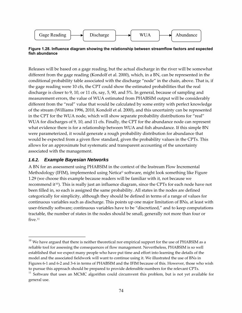
Abundance WUA Discharge Gage Reading

Figure 1.28. Influence diagram showing the relationship between streamflow factors and expected fish abundance

Releases will be based on a gage reading, but the actual discharge in the river will be somewhat different from the gage reading (Kondolf et al. 2000), which, in a BN, can be represented in the conditional probability table associated with the discharge “node” in the chain, above. That is, if the gage reading were 10 cfs, the CPT could show the estimated probabilities that the real discharge is closer to 9, 10, or 11 cfs, say, 5, 90, and 5%. In general, because of sampling and measurement errors, the value of WUA estimated from PHABSIM output will be considerably different from the “real” value that would be calculated by some entity with perfect knowledge of the stream (Williams 1996, 2010, Kondolf et al. 2000), and this uncertainty can be represented in the CPT for the WUA node, which will show separate probability distributions for “real” WUA for discharges of 9, 10, and 11 cfs. Finally, the CPT for the abundance node can represent what evidence there is for a relationship between WUA and fish abundance. If this simple BN were parameterized, it would generate a rough probability distribution for abundance that would be expected from a given flow standard, given the probability values in the CPTs. This allows for an approximate but systematic and transparent accounting of the uncertainty associated with the management.

1.6.2. Example Bayesian Networks A BN for an assessment using PHABSIM in the context of the Instream Flow Incremental Methodology (IFIM), implemented using Netica© software, might look something like Figure 1.29 (we choose this example because readers will be familiar with it, not because we recommend it10). This is really just an influence diagram, since the CPTs for each node have not been filled in, so each is assigned the same probability. All states in the nodes are defined categorically for simplicity, although they should be defined in terms of a range of values for continuous variables such as discharge. This points up one major limitation of BNs, at least with user‐friendly software; continuous variables have to be “discretized,” and to keep computations tractable, the number of states in the nodes should be small, generally not more than four or five.11

10 We have argued that there is neither theoretical nor empirical support for the use of PHABSIM as a reliable tool for assessing the consequences of flow management. Nevertheless, PHABSIM is so well established that we expect many people who have put time and effort into learning the details of the model and the associated fieldwork will want to continue using it. We illustrated the use of BNs in Figures 6‐1 and 6‐2 and 3‐6 in terms of PHABSIM and the IFIM because of this. However, those who wish to pursue this approach should be prepared to provide defensible numbers for the relevant CPTs. 11 Software that uses an MCMC algorithm could circumvent this problem, but is not yet available for general use.

74

DischargeLowMediumHigh

33.333.333.3

Fish_WUALowMediumHigh

33.333.333.3

DepthLowMediumHigh

33.333.333.3

SubstrateFineMediumCoarse

33.333.333.3

VelocityLowMediumHigh

33.333.333.3

Fish_AbundanceLowMediumHigh

33.333.333.3

TemperatureLowMediumHigh

33.333.333.3

Invert_AbundanceLowMediumHigh

33.333.333.3

NutrientsLowMediumHigh

33.333.333.3

Invert_WUALowMediumHigh

33.333.333.3

Figure 1.29. A simple Bayesian Network for an assessment using PHABSIM in the context of the IFIM. The network has not been parameterized, the probabilities of all states are shown as equal. (We use PHABSIM in this example because people are familiar with it, not because we recommend it.)

The probability values in the CPTs can be estimated from data, from output of other models, or from professional opinion, which makes BNs useful for integrating different kinds of information from various sources; for example, the CPT for one node could be estimated from data, while that for another could be estimated from expert opinion. To illustrate ‘parameterizing’ CPTs from data, we have developed a BN for the abundance of brown and rainbow trout in Martis Creek in Nevada and Placer Counties,12 using Netica© software and data from thirty years of monitoring by PBM and his students (Figure 1.30). We defined the influence diagram (the boxes and arrows), and the CPTs were derived by the software from the data.

As it appears in Figure 1.30, the BN simply summarizes the information in the data, for example that the highest flow came in spring in 27% of years. The probabilities shown for the “child” nodes (those with arrows running to them) are conditional on both the data and the model. To use the model, the user could introduce a “finding,” say that the mean annual flow was low. This would change the probability of that state to 100%, and the model would adjust the

12 More traditional analyses of these data are reported in Kiernan and Moyle (see section 3.0).

75

probabilities of the states for trout density accordingly (but not much, in this case, e.g., the probability of ‘high’ brown trout density decreases to 32.3%). Note also that the arrows do not necessarily imply causation, only association.

Rainbow trout densityHighModerateLow

33.331.535.2

24.8 ± 29

Mean annual flowLowNormalHigh

27.648.324.1

1.75 ± 2.5

Mean stream depth (m)ShallowIntermediateDeep

24.639.436.0

0.704 ± 0.85

Brown trout densityHighModerateLow

34.429.336.3

182 ± 290

Timing of max flow (season)WinterSpring

73.126.9

Dominant habitat typeRiffleRunPoolNone

7.3970.921.7 0 +

Dominant substrate typefinegravelcobbleboulderNone

3.5510.978.5 0 +7.09

Figure 1.30. A simple Bayesian network showing factors that determine brown trout and rainbow trout density (mostly young-of-the-year) in Martis Creek, California. Conditional probability tables associated with each node (i.e., variable) in the network were derived from data collected from 1979-2008. The networks can also include nodes representing decisions and utilities (costs or benefits), in which case they may be called Bayesian decision networks (BDNs). In the current context, the potential states of a decision node might be flow regimes, and the utility nodes might represent power generation, the value of the fishery, fish populations, some measure of biodiversity, etc. Importantly, the BN would not generate point estimates of these utilities, but rather, approximations of the probability distributions of the utilities.

Where multiple projects will be coming up for licensing or re‐licensing within a region, as with the Sierra Nevada and Cascade Mountains, FERC or another agency such as the California Energy Commission (CEC) could support the development of a set of template BNs that could be used as a starting point in each process. Figures 1.31 and 1.32 represent first stabs at the influence diagrams for such BNs. These should be developed and reviewed by knowledgeable scientists in a somewhat formal process with peer review, as described by Marcot et al. (2008), which would allow increased confidence that the BNs actually reflect current understanding of

76

the relevant ecology or other sciences. The BNs could be refined based on monitoring data, and used in adaptive management approaches as described in section 1.5. The BNs would also provide a means by which information from various streams can be combined, so that monitoring data collected on one stream can be used to improve assessments in others. In an earlier PIER study for the CEC, Cox (2007) identified a need for increased consistency in study protocols; template BNs would help meet this need.

Primary_Productivitystate0 100

Secondary_Productivitystate0 100

Temperature_Regimestate0 100

Light_on_Streamstate0 100

Nutrientsstate0 100

Channel_TypeAlluvialSemi ConfinedConfined

33.333.333.3

Riparian_Vegstate0 100

Gradientstate0 100

Flow_Regimestate0 100

Aspectstate0 100

Geologystate0 100

Figure 1.31. A simple Bayesian Network for primary and secondary productivity in a Sierran stream. Finally, as the name suggests, BNs are compatible with Bayesian statistical modeling, particularly hierarchical Bayesian (HB) modeling. Where reducing continuous variables to a set of discrete ranges seems too unsatisfactory, and adequate data are available, HB modeling can be used to explore particular parts of a BN.

77

Channel_Morphologystate0 100

Foodstate0 100

Flow_Regimestate0 100

Aspectstate0 100

Temperature_Regimestate0 100

Trout_Productivitystate0 100

Gradientstate0 100

Substratestate0 100

Riparian_Vegstate0 100

Water_Qualitystate0 100

Land_Usestate0 100

Disturbance_Regimestate0 100

Figure 1.32. A simple Bayesian Network for trout productivity in a Sierran stream.

78

1.7. Summary conclusions and recommendations 1.7.1. Summary Conclusions 1. Environmental Flow Assessment (EFA) remains a difficult problem for which there is no

convenient solution; a high quality assessment requires a better understanding of how streams ecosystems work than we have, despite the great amount of knowledge that is available. Given the complexity of ecosystems, this should not be a surprise. The challenge is how to make responsible decisions about the allocation of water between instream and other uses in the face of incomplete understanding. Doing this requires that uncertainty be acknowledged and addressed.

2. There is abundant evidence that stream ecosystems and their fish populations are highly variable and are not equilibrium systems (Mangel et al. 1996, Power et al. 2008), and that biological as well as physical factors structure ecosystems (Power et al. 2008). Food often limits populations, especially for stream salmonids (Wipfli and Baxter 2010). Fish are affected by factors operating at multiple spatial and temporal scales (Cooper et al. 1998, Anderson et al. 2006, Armstrong 2010), so there is no single “right” spatial or temporal scale at which to conduct an assessment.

3. Abundance‐environment relations (AERs) that relate physical habitat variables to fish or invertebrate abundance have a limited role to play in EFA (Lancaster and Downs 2010a, 2010b; section 1.4). AERs developed from observational studies do not show causation or even real preference. Moreover, habitat selection is affected by myriad factors including discharge (section 1.3). The AERs used in PHABSIM have been the subject of considerable criticism, and better methods for developing AERs, such as logistic regression, are more defensible from a statistical point of view. However, these methods do not overcome the basic limitations of AERs for assessing habitat quality.

4. Habitat association models such as PHABSIM that infer habitat quality from AERs are based on outdated concepts and unsupported assumptions, do not deal with the processes that actually control populations, and have dubious utility for estimating the future abundance of biomass of the target organisms (Anderson et al. 2006, Armstrong 2010, Lancaster and Downes 2010a, 2010b), especially in response to changes in flow. Published tests claiming to show strong relationships between populations or biomass and the habitat index estimated by PHABSIM are mostly flawed, and better tests show weak or no relationships (Appendix A).

5. Long‐term data sets with which critical hypotheses can be assessed are necessary to develop the improved scientific understanding upon which effective EFAs must be based. Monitoring below hydroelectric facilities can provide such data, provided it is properly designed and adequately funded.

6. Bayesian Networks appear to be a useful method for integrating various kinds of information regarding environmental flows (Hart and Polino 2009), and for guiding the development of study plans and monitoring programs.

79

7. Except for habitat‐association models, statistical and ecological modeling is seldom used effectively in EFA in the USA. This suggests that holistic approaches that include the use of expert opinion are likely to be most effective in designing environmental flow regimes.

1.7.2. Recommendations Manage adaptively Like others, we recommend an adaptive approach to management of environmental flows. To make adaptive management effective, decision‐makers should be explicit about the reasoning underlying their decision, so that it is clear what kind of new information would justify a change in the decision. In the current context, the decision should articulate what the specified environmental flows are intended to achieve, stated both in terms of policy objectives and also measurable performance criteria. (This applies as well to the parties in the alternative licensing process, if they recommend environmental flows and related mitigation conditions for adaption by FERC). The decision should provide for monitoring that is good enough to tell whether the performance criteria are satisfied, and to test the rationale upon which the flow decision was based.

Manage for the ecosystem Environmental flow assessment should take a holistic approach, like that embedded in the DRIFT framework. That is, management should consider the effects of the project on all aspects of the ecosystem, including nutrient sources and food webs, not just selected species.

Try Bayesian Networks To further an adaptive and holistic approach, try Bayesian Networks. To further consistency in ILP study programs, support development of a set of template Bayesian Networks that can be used and adapted by participants in the FERC integrated licensing process. The template BNs should be developed and reviewed by area experts (Marcot et al. 2006), and be revised and updated as new information and understanding develops, or to fit conditions in particular streams or basins. Bayesian networks will not provide easy answers, but they do promise to

• Make adaptive management more rigorous and speed adaptive learning;

• Allow for integrating various types of information;

• Provide an efficient means to incorporate new knowledge into assessments;

• Display the uncertainty in assessments.

Make better use of modeling and statistics Insist on interval estimates (e.g., estimates with confidence intervals), rather than point estimates. Interval estimates have been basic to science for many decades.

Beware of models that promise too much Experience shows that things that seem too good to be true usually are, and this applies to models as much as anything else. Given the complexity of ecosystems, models or methodologies that claim to provide managers with just what they need to make judgments about environmental flows should be regarded with considerable skepticism.

80

Distinguish science and dispute resolution Environmental flow assessment normally occurs in the context of disputes over the allocation of water, so inevitably EFMs will be judged in the context of dispute resolution as well as on their scientific merit, but it is important to keep these considerations separate. Scientific questions cannot be answered by agreement of the parties involved.

1.7.3. Concluding remark Given the complexity of flow in streams described in section 1.3, and the crude representation of them by 1‐D CDF models, together with what was known about habitat selection by the 1970s, it may seem strange that methods such as PHABSIM became so well established. However, this is not really such an anomaly. In the preface to their book on ecological modeling, Hilborn and Mangel (1997) described complaints from colleagues that a beta‐test version of the book presented models that were too simple and unrealistic for anyone to take them seriously. Hilborn and Mangel responded that, “This charge is unfair. These apparently ridiculous models were in fact proposed and used by pretty smart people. Why? Because they had no alternative model. … If there is only one model, it will be used; …” We think this has been the situation with EFA and PHABSIM.

81

2.0 Retrospective Analysis of Environmental Flows and Fish Monitoring in FERC Licensing Joseph D. Kiernan, Center for Watershed Sciences, University of California, One Shields Avenue, Davis, CA 95616. [email protected]

2.1. Introduction and Approach 2.1.1. Regulatory mandates and hydropower licensing Under the Federal Power Act of 1935 (FPA), the Federal Energy Regulatory Commission (hereafter Commission or FERC) is charged with determining “whether, and under what conditions, to issue licenses for the construction, maintenance, and operation, or continued operation, of non‐federal hydropower facilities.” As such, the Commission has a statutory mandate requiring that all hydropower licenses contain conditions that will be:

[B]est adapted to a comprehensive plan for improving or developing a waterway or waterways for the use or benefit of foreign commerce, for the improvement and utilization of water‐power development, for the adequate protection, mitigation, and enhancement of fish and wildlife (included related spawning grounds and habitat), and for other beneficial public uses, including irrigation, flood control, water supply, and recreational and other purposes (FPA 2006: 16 U.S.C. §803(a)(1)).

A 1986 amendment to the FPA13 elevated the role of ecological considerations in the licensing process. Specifically, the amendment requires FERC to solicit recommendations of state and federal resource agencies for the protection of fish, wildlife, and other natural resources. Such recommendations fall under Section 10 of the FPA and are included as conditions in all new licenses, unless FERC deems them inconsistent with the FPA or other applicable law, and there are alternative conditions or measures that will adequately address fish and wildlife issues. Additionally, section 4(e) of the FPA requires that FERC licenses for projects located within federal reservations must include all terms and conditions that the Secretary of the department under whose supervision the reservation falls shall deem necessary for the adequate protection and utilization of such reservation. .

2.1.2. Adequate protection, mitigation, and enhancement Since new licenses issued by FERC range between 30 and 50 years in term, inadequate measures to protect, mitigate, or enhance fish and wildlife populations have the potential to be in place for many years (Pollak 2009). License conditions that mandate changes in flow regime, in particular, are routinely based on models (e.g., IFIM, PHABSIM and similar models; see section 1.4) that predict local responses by aquatic biota to the amount of available water. However, such predictions are increasingly being recognized as hindered by unsupported assumptions (Kondolf et al. 1987), frequently biased (Williams 1996) and, above all, fraught with uncertainty (Williams 2010). Not surprisingly, post‐license monitoring of aquatic resources, often under the label of adaptive management, is commonly included as a condition of a new license to assess

13 The Electric Consumer Protection Act.

82

ecological response to a new flow regime. For fish populations in hydropower affected streams, typical variables to be monitored might include population size, distribution, and condition, and such information would be used to guide and potentially alter instream flow releases and other operational conditions set forth in a new license. Yet true adaptive management, as defined by Williams et al. (2009: 1) is “a systematic approach for improving resource management by learning from outcomes.” Learning, in this context, requires continuous monitoring and evaluation of fish population status and trends, and a significant investment of both time and money on the part of the licensee. Perhaps more importantly, it requires implementation of a scientifically rigorous monitoring program with explicitly defined objectives and performance criteria (Marshall et al. 2008).

2.1.3. Fish and FERC licensing in California The decline of California’s native fish fauna has been well documented (Moyle and Williams. 1989, Moyle et al. 1995). In a recent assessment, Moyle et al. (forthcoming) reported that 54% of California’s extant native inland fishes are seriously imperiled, with another 25% of the species presently in decline or otherwise of special concern. Among myriad factors contributing to this decline are dams that alter natural flow regimes, impede the movement of organisms and material, and alter ecological processes. An increased awareness of the potentially negative ecological consequences associated with hydropower projects has led to the inclusion of mitigation measures in FERC issued licenses. In California and elsewhere, releases of water from dams to downstream environments are frequently mandated in new licenses granted to operators of hydropower facilities. Often, the primary objective of flow releases is to maintain or enhance native fish communities, or important recreational fish species, by increasing the occurrence of successful spawning and recruitment (Tharme 2003, Huckstorf et al. 2008). The success or failure of this objective can only be assessed through rigorous monitoring of spatial and temporal trends in species abundance and assemblage composition.

Here we provide a brief review of thirteen recent FERC hydropower licensing proceedings in California (Table 2.1). Our primary purpose is to determine whether fish monitoring is routinely mandated in new FERC licenses for operation, and how useful the information collected is likely to be in determining effects of the dams. Each case study includes a brief description of the physical setting and infrastructure associated with the project, as well as information regarding fish monitoring conducted both before and after environmental (instream) flows were implemented, when applicable. Documents, filings and other resources used to compile each case study were obtained from the FERC Online electronic library (formerly called FERRIS; http://www.ferc.gov) using the advance search option.

83

http://www.ferc.gov/

Table 2.1. Hydropower licensing proceedings used to assess contemporary trends in environmental flow assessment and post-license fisheries monitoring requirements.

FERC FERC Issuance Expiration AuthorizedProject Project Name Waterway Licensee date date (KW)02100 Oroville Facilities Feather River California Dept. Water Resources Pending 1/31/2007 76285000233 Pit 3, 4, & 5 Pit River Pacific Gas and Electric Co. 7/2/2007 6/30/2043 31233000184 El Dorado South Fork American R. El Dorado County Irr District 10/18/2006 9/30/2046 2100000382 Borel Kern River Southern California Edison Co. 5/17/2006 4/30/2046 1200002067 Tulloch Stanislaus River Oakdale & San Joaquin Irr Dist 2/16/2006 12/31/2046 2410002005 Beardsley/Donnells Middle Fork Stanislaus R. Oakdale & San Joaquin Irr Dist 1/30/2006 12/31/2046 8250000372 Lower Tule River Middle Fork Tule R. Southern California Edison Co. 9/3/2004 8/31/2034 252002017 Big Creek No 4 San Joaquin River Southern California Edison Co. 12/4/2003 11/30/2039 9882201354 Crane Valley Willow Creek Pacific Gas and Electric Co. 9/16/2003 8/31/2043 2870002699 Angels Angels Creek Utica Power Authority 9/3/2003 8/31/2033 140011563 Upper Utica Silver Creek Northern California Power Agency 9/3/2003 8/31/2033 002019 Utica Silver Creek Utica Power Authority 9/3/2003 8/31/2033 450001934 Mill Creek 2/3 Mountain Home Creek Southern California Edison Co. 7/22/2003 6/30/2033 3000

2.2. Case Studies 2.2.1. Oroville Facilities (FERC Project Number 2100) Introduction: The Oroville Hydropower Facilities encompass ca.166 km2 within the Feather River watershed in Butte County, California. The facilities include Oroville Dam (2,317 m long × 235 m high) and Reservoir (3.5 maf storage), three power plants, Thermalito Diversion Dam (396.2 m long × 43.6 m high), the Feather River Fish Hatchery and Fish Barrier Dam, Thermalito Power Canal (3,048 m long), Oroville Wildlife Area, Thermalito Forebay (max. operating storage = 11,770 acre‐feet), and Thermalito Afterbay (max. operating storage = 57,040 acre‐feet).

The Oroville Facilities are operated by the California Department of Water Resources (DWR) for water storage and delivery, power generation, flood control, water quality improvement in the Sacramento‐San Joaquin Delta, recreation, and enhancement of fish and wildlife (DWR 2004). During operation, the majority of the Feather River below Oroville Dam is diverted at the Thermalito Diversion Dam into Thermalito Afterbay and Thermalito Forebay and eventually released back into the Feather River at the Thermalito Afterbay Outlet, approximately 14.5 km downstream (DWR 2010). The project‐affected section of the Feather River between the Fish Barrier Dam and the Thermalito Afterbay Outlet is designated as the low flow channel (LFC). The Fish Barrier Dam, ca. 0.6 km downstream of the Thermalito Diversion Dam, blocks the upstream migration of fish. DWR operates and maintains the Oroville Facilities under the terms and conditions of an existing FERC license (issued 11 February 1957; effective 1 February 1957), which expired on 31 January 2007. The Oroville facilities have since been operating under annual licenses issued by FERC.

Flow regime: The Oroville Facilities are operated to meet minimum instream flow requirements in the Lower Feather river, as established by an agreement between DWR and the California Department of

84

Fish and Game (CDFG). The 1983 agreement specifies that the Facilities release a minimum flow of 17 m3/s (600 cfs) into the LFC for fisheries purposes. The Thermalito Afterbay Outlet is also operated to meet minimum instream flow requirements for the river downstream from the outlet, (known as the high flow channel; HFC) (Table 2.2), in addition to water demands for State Water Project delivery and Delta environmental protection.

Table 2.2. Lower Feather River minimum flow requirements (cfs) downstream of the Thermalito Afterbay. Table modified from DWR (2007).

Normal Runoff 1 Oct. – Feb. Mar. Apr. – Sep. > 55% 1,700 1,700 1,000 < 55% 1,200 1,000 1,000

1Defined as the mean April through July unimpaired runoff near Oroville for the period 1911‐1960. Fish assemblages: Normal operation of the Oroville Project potentially affects environmental conditions within the Lower Feather River, as well as Lake Oroville and its upstream tributaries, the Diversion Pool, Thermalito Forebay, Thermalito Aflerbay, the Feather River fish hatchery, the Fish Barrier Pool, and the Oroville Wildlife Area ponds (DWR 2005). Information regarding fish assemblages in these habitats was compiled from snorkel surveys, beach seining, trapping, field observations and historical accounts. The warm and coldwater fish species in each of the major project‐affected areas are presented in Table 2.3. Of special significance are the three ESA‐listed species (spring‐run Chinook, steelhead trout, and green sturgeon) and three CDFG fish species of concern (river lamprey, hardhead, and Sacramento splittail). The Feather River fish hatchery, constructed in 1967, produces and releases both endangered salmonid species as well as fall‐run Chinook, and is the only hatchery in the Central Valley producing spring‐run Chinook salmon (DWR 2007).

Instream flow assessment: The Physical Habitat Simulation (PHABSIM) model was used to assess the relationship between instream flows and habitat suitability for various life stages (i.e., spawning, juvenile rearing and juvenile emigration) of Chinook salmon and steelhead trout (DWR 2007). Habitat suitability was determined in two segments of the Lower Feather River: 1) the LFC and 2) the HFC down to the confluence with Honcut Creek (DWR 2007).

85

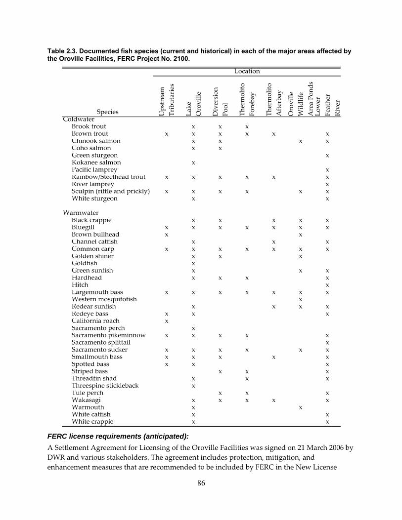
Table 2.3. Documented fish species (current and historical) in each of the major areas affected by the Oroville Facilities, FERC Project No. 2100.

Upstream

Tributaries

Lake

Oroville

Diversion

Pool

Thermolito

Forebay

Thermolito

Afte

rbay

Oroville

Wild

life

Area Po

nds

Lower

Feather

River

ColdwaterBrook trout x x xBrown trout x x x x x xChinook salmon x x x xCoho salmon x xGreen sturgeon xKokanee salmon xPacific lamprey xRainbow/Steelhead trout x x x x x xRiver lamprey xSculpin (riffle and prickly) x x x x x xWhite sturgeon x x

WarmwaterBlack crappie x x x x xBluegill x x x x x x xBrown bullhead x xChannel catfish x x xCommon carp x x x x x x xGolden shiner x x xGoldfish xGreen sunfish x x xHardhead x x x xHitch xLargemouth bass x x x x x x xWestern mosquitofish xRedear sunfish x x x xRedeye bass x x xCalifornia roach xSacramento perch xSacramento pikeminnow x x x x xSacramento splittail xSacramento sucker x x x x x xSmallmouth bass x x x x xSpotted bass x x xStriped bass x x xThreadfin shad x x xThreespine stickleback xTule perch x x xWakasagi x x x x xWarmouth x xWhite catfish x xWhite crappie x

Species

Location

x FERC license requirements (anticipated): A Settlement Agreement for Licensing of the Oroville Facilities was signed on 21 March 2006 by DWR and various stakeholders. The agreement includes protection, mitigation, and enhancement measures that are recommended to be included by FERC in the New License

86

when issued. With respect to the flow regime, Article A108.1 proposes a minimum flow increase to address habitat and temperature needs of anadromous salmonids. Minimum flows in the low flow channel will increase from 17.0 to 19.8 m3/s (600 to 700 cfs) from 1 April to 8 September, and to 22.6 m3/s (800 cfs) from 9 September to 31 March to facilitate spawning by anadromous fish. Flows in the high flow channel (Article A108.2) remain unchanged, as established in the 1983 DWR and CDFG agreement (DWR 2006).

Post-licensing fisheries monitoring (anticipated): The Lower Feather River Habitat Improvement Plan includes nine component programs intended to ameliorate ecological conditions in the Lower Feather River for anadromous salmonids and other aquatic biota. The nine programs are:

1. Gravel Supplementation and Improvement Program

2. Channel Improvement Program

3. Structural Habitat Supplementation and Improvement Program

4. Fish Weir Program

5. Riparian and Floodplain Improvement Program

6. Feather River Fish Hatchery Improvement Program

7. Instream Flow and Water Temperature Requirements for Anadromous Fish

8. Comprehensive Water Quality Monitoring Program

9. Oroville Wildlife Area Management Plan

For each component program, DWR will prepare and submit an annual report of monitoring results and activities for the first five years after the new FERC license is issued. After the fifth year, DWR will consolidate the component reports into a single, comprehensive monitoring and adaptive management summary report to be prepared every five years for the remainder of the License term (DWR 2007).

2.2.2. Pit 3, 4, 5 Hydropower Project (FERC Project Number 233-081) Introduction: The Pit 3, 4, 5 Hydropower Project is operated by Pacific Gas and Electric Company (PG&E) on the Pit River in Shasta County, California. The Project comprises three hydraulically connected developments and includes, in part, four dams and reservoirs, three powerhouses, and associated tunnels, surge chambers, and penstocks. The Pit 3 development is located furthest upstream and consists of the 523.3 ha Lake Britton, (gross storage capacity = 5.2 ×107 m3 [41,877 acre‐feet]), the Pit 3 Dam (150.6 m crest length × 39.6 m high), a concrete tunnel (in two sections; total length ca. 6.4 km), a surge tank, three penstocks (ca. 3.1 m diameter × 182.9 m in length), a powerhouse, a fish barrier dam located on Hat Creek, and other facilities.

87

The Pit 4 development consists of the Pit 4 Dam14 and reservoir (42.5 ha; storage capacity = 2.4 ×106 m3, [1970 acre‐feet]), a pressure tunnel (5.8 m diameter; total length = 6.6 km), a surge chamber, two penstocks (3.7 m diameter; ca. 243.8 m in length), a reinforced concrete powerhouse and other appurtenant facilities. The Pit 5 development is the downstream‐most development and consists of the Pit 5 Dam (103.6 m long × 20.4 m max. height) and Reservoir (13.0 ha; storage capacity = 3.9 ×105 m3, [202 acre‐feet]), Tunnel No.1 (5.8 m dia. × 1.6 km in length), the Pit 5 Tunnel Reservoir (19.4 ha; storage capacity = 1.3 ×106 m3, [645 acre feet) and Dam, (ca. 944.9 m long × 20.1 m high), the Pit 5 Tunnel No. 2 (5.8 m dia. × 7.0 km in length), a surge chamber, four steel penstocks (ca. 2.4 m diameter × 426.7 m long), a powerhouse and associated infrastructure.

Flow regime: During normal operation, PG&E maintained a year‐round minimum release flow of 4.2 m3/s (150 cfs) to the Pit 3 bypassed reach. When combined with tributary inputs and spring accretion, this release yielded flows in the lower third of the reach that ranged from ca. 5.8 m3/s (205 cfs) during September and October to > 8.5 m3/s (300 cfs) during February and April, excluding spill events. Releases to the Pit 4 bypassed reach were also maintained at 4.2 m3/s (150 cfs) year‐round, which, when combined with tributary inputs and accretion, provided flows in the lower portion of the reach that range from ca. 5.9 m3/s (210 cfs) during September and October to > 7.8 m3/s (275 cfs) during February and April, excluding spill events. Finally, minimum flow releases to the Pit 5 reach were maintained at 2.8 m3/s (100 cfs) year round, which resulted in flows in the lower portion of the reach that ranged from 4.5 m3/s (158 cfs) during September and October to > 18.4 m3/s (650 cfs) during February and April, excluding spill events.

Fish assemblages: Fish populations in the bypassed reaches were initially characterized from historical accounts and snorkel surveys conducted in 1983‐84 and 1987‐92 that targeted rainbow trout, Sacramento sucker, Sacramento pikeminnow, and hardhead (PG&E 2001b). FERC subsequently requested that additional sampling be conducted due to a significant change to the flow regime in 1987 and the known presence of rare fish species in the Pit River. In 2002, upper and lower sections of each bypassed reach were sampled via electrofishing and snorkel surveys to provide information on fish community composition, density, relative abundance and size distribution (Stillwater Environmental Services 2002). A list of species occurring in project‐affected waterways is provided in Table 2.4.

14 The Pit 4 dam consists of a gravity type overflow section 61.9 m in length with a maximum height of 32.9 m and a slab‐and buttress type section 64.6 m in length with a maximum height of 23.8 m.

88

Table 2.4. Fish species identified in waterways associated with the Pit 3, 4, 5 Hydroelectric Project.

Species Lake

Brit

ton

Pit

4 re

serv

oir

Pit

5 re

serv

oir

Tunn

el re

serv

oir

Pit

3 by

pass

ed re

ach

Pit

4 by

pass

ed re

ach

Pit

5 by

pass

ed re

ach

Native

Bigeye marbled sculpin x x x x x x Hardhead x x x x x x x Pit/Klamath brook lamprey x x x x Northern roach x x x x x x x Pit sculpin x x x x x x x Rainbow trout x x x x x x x Rough sculpin x x x x Sacramento pikeminnow x x x x x x x Sacramento sucker x x x x x x x Speckled dace x x x x x x x Tui chub x Tule perch x x x x x x x Non‐native Black bullhead x Black crappie x x x x Bluegill x x x x Brown bullhead x Brown trout x x x Common carp x x Channel catfish x Golden shiner x x x Green sunfish x x Largemouth bass x x x Smallmouth bass x x x White crappie x x x

Instream flow assessment: As summarized in the license application (i.e., PG&E 2001), PG&E employed standard Instream Flow Incremental Methodology (IFIM; referred to as 1D) procedures to examine the effects of alternative release flows on the amount of physical habitat available to rainbow trout,

89

Sacramento sucker, Sacramento pikeminnow, and hardhead in each bypassed reach. In 1984, multiple transects were established in riffle and run habitats in upper and lower segments of each bypassed reach, and a single transect was placed in a pool in each reach. Depths and velocities were then measured at target flows of ca. 1.4, 2.8, 4.2, and 8.5 m3/s (50, 100, 150, and 300 cfs, respectively) and used to assess hydraulic conditions up to a maximum flow of 17.0 m3/s (600 cfs). In 2002, PG&E subsequently re‐analyzed and submitted updated microhabitat suitability curves for hardhead and rainbow trout that accounted for the current flow regime in project‐affected reaches.

FERC license requirements: A new 40‐year license was issued to PG&E for continued operation of Pit 3, 4, 5 on 2 July 2007. The license established new minimum stream flows for the Pit 3, Pit 4, and Pit 5 bypassed reaches. Specific conditions of the required minimum stream flows are provided in Table 2.5. As a technical note, spill events for each bypassed reach were formally defined as a three‐day mean flow of > 8.5 m3/s (300 cfs) above the new required minimum streamflow that lasts for three consecutive days (FERC 2007a).

Among the mitigation and enhancement measures included in the new License, article 401 and the State’s Water Quality Certification (Appendix A, Condition 14, Measure 3), required PG&E to develop and implement a fish and invertebrate monitoring plan. Specifically, Measure 3 (FERC 2007: 95) stated, in part, that:

PG&E shall develop and implement a fish and invertebrate monitoring plan that is based on the methods used in surveys conducted during the licensing effort and the current Biological Compliance Monitoring Plan (BCMP), including angler surveys, reservoir fish surveys, river reach surveys, macroinvertebrate surveys, and aquatic mollusk surveys. This plan shall be developed within six months of license issuance, and for surveys in years 1 through 4 and in years 8, 12, 16, 20, and 24….

Additionally, Article 405 and Condition 23(b) of the Forest Service’s (2003) mandatory terms and conditions required that PG&E work with a Technical Review Group (TRG15) to prepare a River Fish Monitoring Plan to monitor the status of the fish populations and the trout fishery in the three project bypassed reaches under the new minimum instream flows required by the License. Condition 23(b) further required that a technical report be prepared following each sampling effort that describes and discusses: 1) survey results and how they compare with those of previous surveys, 2) trends in fish abundances, 3) trends for entrained Forest Service special status fish species, 4) changes to bald eagle prey species, and 5) any evidence that non‐native bass are expanding into project reaches (USFS 2003). 15 Appendix B Condition 23 (a) of the new License required the establishment of a Technical Review Group (TRG) to consult with PG&E regarding the design of management and monitoring plans, data review and evaluation, and adaptive management plans. The TRG was required to include representatives from the FS, CDFG, CWRCB, FWS, National Park Service, Tribal governments, and non‐governmental organizations.

90

Table 2.5. Summary of minimum stream flows required in the bypassed stream reaches associated with Pit 3, 4, 5 (Source: FERC 2007a).

Location Season Start date: End date: m3/s (cfs)Pit 3 reach Summer 21 Apr 31 Aug 8.5 (300)

Fall 1 Sep Between 1 Nov and 30 Nov

7.9 (280)

Winter (after spill occurs) Between 1 Nov and 20 Apr

20 Apr 9.9 (350)

Winter (prior to spill) 1 Dec 20 Apr 8.5 (300)

Winter spill cessation Between 16 Mar and 15 Jun

15 Jun Following cessation 14 days at 12.7 (450)14 days at 11.3 (400)10 days at 9.9 (350)

then: 8.5 (300)

Pit 4 reach Summer 16 Jun 31 Aug 10.6 (375)

Fall 1 Sept Between 1 Nov and 30 Nov

9.9 (350)

Winter (after spill occurs) Between 1 Nov and 15 Jun

15 Jun 12.7 (450)

Winter (prior to spill) 1 Dec 15 Jun 10.6 (375)

Winter spill 16 Mar 30 Apr 17.0 (600)

Cessation 1 May 31 May 15.6 (550)1 Jun 15 Jun 14.2 (500)

Pit 5 reach Summer 21 Apr 31 Aug 11.3 (400)

Fall 1 Sep Between 1 Nov and 30 Nov

9.9 (350)

Winter (after spill occurs) Between 1 Nov and 20 Apr

20 Apr 12.7 (450)

Winter (prior to spill) 1 Dec 20 Apr 11.3 (400)

Winter spill cessation Between 16 Mar and 15 Jun

15 Jun Following cessation 14 days at 15.6 (550)10 days at 14.2 (500)10 days at 12.7 (450)

then: 11.3 (400)

Required minimum flow

PG&E subsequently filed four resource‐specific monitoring plans: a Reservoir Fish Monitoring Plan; a River Fish Monitoring Plan; an Aquatic Mollusk Monitoring Plan; and a River Macroinvertebrate Monitoring Plan. With respect to riverine fishes, PG&E proposed to document and monitor the status of fish populations under the new minimum instream flows in the Pit River below Lake Britton, below Pit 4 forebay, and below Pit 5 forebay (FERC 2009).

91

Sampling efforts will specifically target rainbow trout, Sacramento sucker, hardhead, Sacramento pikeminnow, and tule perch (FERC 2009).

Post-licensing fisheries monitoring: No post‐license fisheries monitoring has been conducted. Surveys are required to begin in 2011 (the first year of full minimum flow releases) and continue for 5 consecutive years, with sampling occurring every fourth year thereafter (FERC 2009).

2.2.3. El Dorado Hydroelectric Project (FERC Project Number 184) Introduction: The El Dorado Hydroelectric Project is located on the South Fork of the American River (SFAR) and its tributaries in Alpine, Amador, and El Dorado counties, California. The project is operated by El Dorado Irrigation District and includes four storage reservoirs and 16 dams (height range = 0.5 m to 21.2 m) that divert water to the SFAR. The four storage reservoirs capture water from the Truckee and American River watersheds and release this water directly into the SFAR, its tributaries, or a conduit (detailed below). Flows are then diverted by the El Dorado Diversion Dam on the SFAR into the 35.9 km long El Dorado Canal. The El Dorado Canal has a maximum hydraulic capacity of 4.7 m3/s and flows in the canal are augmented by 7 tributaries of the SFAR16. The actual volume of water diverted at the diversion dam is dependent upon the volume of flow contributed by the tributaries. At the terminus of the El Dorado Canal a dam creates El Dorado Forebay which serves as a reservoir for the El Dorado Powerhouse. The powerhouse discharges back into the SFAR at Slab Creek Reservoir which is licensed as part of the Sacramento Municipal Utility District American River Project (FERC project number 2100). The four project storage reservoirs are:

1. Lake Aloha (274.7 ha; usable storage = 6.4 × 106 m3 [5,179 acre‐feet]) formed by a main dam and 11 auxiliary dams which capture water in the low lying areas around the lake. Water is released from Aloha Lake to Pyramid Creek which flows approximately 7.4 km before joining the SFAR.

2. Echo Lake (149.6 ha; usable storage = 2.4 × 106 m3 [1,943 acre‐feet]) is formed by a 97.5 × 4.3 m dam. Echo Lake is unique in that it is the only project‐related reservoir located in the Truckee River Watershed. Water is released through the dam into the 1866.9 m long Echo Lake conduit and ultimately delivered to the SFAR.

3. Caples Lake (298.8 ha; useable storage = 2.5 × 107 m3 [20,338 acre‐feet]) is formed by a 365.8 m long × 25.8 m high main dam and 50 m long auxiliary dam. During periods when inflow to Caples Lake exceeds capacity of the outlet (May through July of some water years), flow is released from a spillway at the auxiliary dam into Caples Creek. Operation of Caples Lake generally reduces instream flows in the spring and increases flows in the summer. At the

16 Alder Creek, Bull Creek, Carpenter Creek, Esmeralda Creek, Mill Creek, Ogilby Creek, and No Name Creek.

92

time of licensing, there was a minimum instream flow requirement of the lesser of 0.14 m3/s (5 cfs) or natural streamflow.

4. Silver Lake (279.9 ha; useable storage = 1.1 × 107 m3 [8,640 acre‐feet]) is formed by a 85.3 m long × 9.1 m high rock and earth dam on the Silver Fork American River.

Flow regime: Under the previous license, the El Dorado Project released from Lake Aloha the lesser of 0.06 m3/s (2 cfs) or inflows during July and August, whereas, water was released from Echo Lake in September through November, with no minimum instream flow requirement. Caples Lake provided a minimum of 0.14 m3/s (5 cfs; or inflow) from August through March, while Silver Lake provided a minimum instream flow of 0.06 m3/s. Continuous minimum instream flows downstream of the El Dorado Diversion dam were previously established for normal and dry years (Table 2.6).

Table 2.6. Existing minimum flow requirements (m3/s) to the bypassed reach from the El Dorado diversion dam (Source: FERC 2003a).

Month of water year Water year type17 Oct Nov Dec Jan Feb Mar Apr May Jun Jul Aug Sep Normal 1.2 1.4 1.4 1.4 1.4 1.4 1.4 1.4 1.4 1.4 1.4 1.1 Dry 0.4 0.5 0.5 0.5 0.5 0.5 0.5 0.5 0.5 0.5 0.5 0.3

No minimum instream flow requirements existed for the seven tributaries that provided water to the El Dorado Canal. Consequently, all streamflow up to 0.43 m3/s could be diverted from Alder Creek and up to 0.28 m3/s could be diverted from each of the other tributaries (i.e., Bull Creek, Carpenter Creek, Esmeralda Creek, Mill Creek, No Name Creek, and Ogilby Creek).

Fish assemblage: Information on fish assemblages in the project‐affected waters was derived from field surveys conducted in 1998‐2000 and historical accounts. Seven native and 7 non‐native species were reported (Table 2.7). Rainbow trout, brown trout, and brook trout are considered indicator species for the Eldorado National Forest and hardhead (reported to occur in the SFAR downstream of the Silver Creek confluence) is designated as a Forest Service sensitive fish species. No state‐listed fish species are known to be present in project waters.

17 Normal year = when SFAR annual runoff at the inflow to Folsom Reservoir was forecasted > 50% of the 50 year average. All other years were classified as “dry.”

93

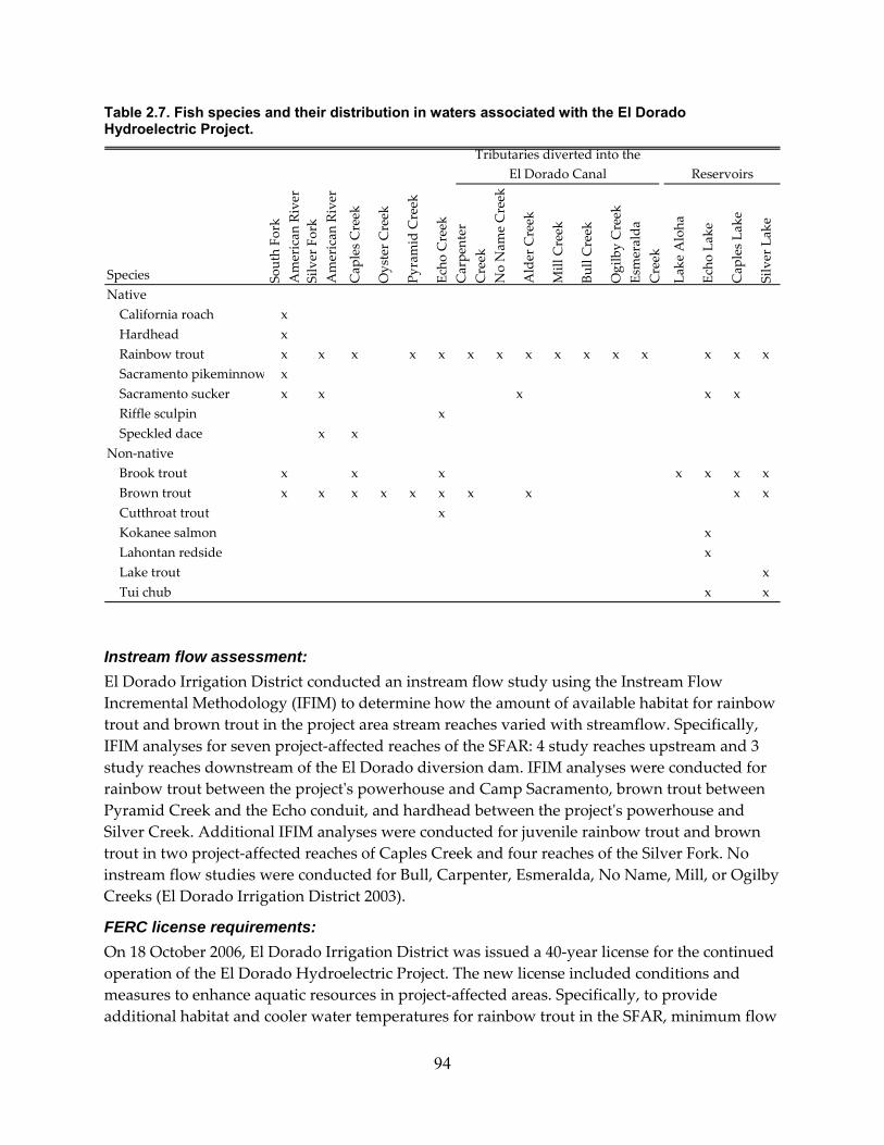
Table 2.7. Fish species and their distribution in waters associated with the El Dorado Hydroelectric Project.

Species South Fo

rk

American River

Silver Fork

American River

Cap

les C

reek

Oyster C

reek

Pyramid Creek

Echo Creek

Carpe

nter

Creek

No Nam

e Creek

Alder Creek

Mill Creek

Bull Creek

Ogilby Creek

Esmeralda

Creek

Lake Aloha

Echo Lake

Cap

les L

ake

Silver Lake

NativeCalifornia roach xHardhead xRainbow trout x x x x x x x x x x x x x x xSacramento pikeminnow xSacramento sucker x x x x xRiffle sculpin xSpeckled dace x x

Non‐nativeBrook trout x x x x x x xBrown trout x x x x x x x x x xCutthroat trout xKokanee salmon xLahontan redside xLake trout xTui chub x x

Tributaries diverted into the El Dorado Canal Reservoirs

Instream flow assessment: El Dorado Irrigation District conducted an instream flow study using the Instream Flow Incremental Methodology (IFIM) to determine how the amount of available habitat for rainbow trout and brown trout in the project area stream reaches varied with streamflow. Specifically, IFIM analyses for seven project‐affected reaches of the SFAR: 4 study reaches upstream and 3 study reaches downstream of the El Dorado diversion dam. IFIM analyses were conducted for rainbow trout between the projectʹs powerhouse and Camp Sacramento, brown trout between Pyramid Creek and the Echo conduit, and hardhead between the projectʹs powerhouse and Silver Creek. Additional IFIM analyses were conducted for juvenile rainbow trout and brown trout in two project‐affected reaches of Caples Creek and four reaches of the Silver Fork. No instream flow studies were conducted for Bull, Carpenter, Esmeralda, No Name, Mill, or Ogilby Creeks (El Dorado Irrigation District 2003).

FERC license requirements: On 18 October 2006, El Dorado Irrigation District was issued a 40‐year license for the continued operation of the El Dorado Hydroelectric Project. The new license included conditions and measures to enhance aquatic resources in project‐affected areas. Specifically, to provide additional habitat and cooler water temperatures for rainbow trout in the SFAR, minimum flow

94

releases downstream of the El Dorado diversion dam were increased to 0.43 to 6.79 m3/s (15 to 240 cfs), depending on month and water year type (FERC 2006e). Similarly, the new license required an increase in minimum flow releases from Lake Aloha to Pyramid Creek ranging from 0.03 to 0.57 m3/s (1 to 20 cfs), and from Echo Lake to Echo Creek ranging from 0.17 to 1.27 m3/s (6 to 45 cfs). The existing 0.14 m3/s (5 cfs) minimum flow release from Caples Lake to Caples Creek was changed to range between 0.14 and 1.56 m3/s (5 and 55 cfs), and the 0.06 m3/s (2 cfs) minimum flow release from Silver Lake to the Silver Fork American River was increased to range between 0.23 and 2.83 m3/s (8 to 100 cfs). Finally, to enhance habitat conditions for rainbow and brown trout below diversion structures in Carpenter, No Name, Mill, Bull, Ogilby, Esmeralda and Alder Creeks, the new license established minimum stream flows for each of these waterways (EID 2003).

Condition No. 37 of the new license required El Dorado Irrigation District to design and implement a monitoring program18. Specific language in the new license stated that (FERC 2006: 76):

Within the scope of the specified monitoring program, the FS [Forest Service], ERC [Ecological Resource Committee19], and SWRCB [State Water Resources Control Board] may select an equal number of alternative years to ensure that surveys occur during a range of water year types. Final study plans shall be approved by the FS, ERC, and SWRCB. The FS, ERC, and SWRCB have the flexibility to alter the monitoring program methodologies and frequencies of data collection if it is determined that: (a) there is a more appropriate or preferable methodology to use than that described in the monitoring plan or (b) monitoring may be reduced or terminated because the relevant ecological resource objective has been met or no change in resource response is expected.

With respect to fishery resources, monitoring of rainbow trout was required during late summer/fall at six locations: 1) SFAR below Carpenter Creek; 2) Lower Alder Creek; 3) Lower Pyramid Creek; 4) Lower Echo Creek; 5) Silver Fork American River at Forgotten Flat; and 6) Caples Creek below Kirkwood Creek. Monitoring was required to be conducted during the first 18 Section 7 (Monitoring Program) of Appendix A to the Settlement, the 401 Certification, and USFS 4(e) conditions required individual study plans for monitoring of the following subjects: Fish Populations; Macroinvertebrates; Amphibians; Riparian Vegetation Species Composition and Recruitment; Geomorphology (Sensitive Site Investigation and Mitigation Plan Development); Geomorphology (Continuing Evaluation of Representative Channel Areas); Water Temperature; Water Quality; Trout Monitoring at Lake Aloha; South Fork American River Flow Fluctuations; EI Dorado Canal Monitoring for Wildlife; Heritage Resource Monitoring; Recreation Survey; Review of Recreation Developments; and Target Lake Levels Evaluation. 19 The ERC is composed of representatives from Forest Service, Park Service, California Dept. of Fish and Game, County of Alpine, County of Amador, El Dorado County Water Agency, E1 Dorado Citizens for Water, Friends of the River, Trout Unlimited, Sierra Club, American Whitewater, Citizens for Water, AKT Development, League to Save Sierra Lakes, Kirkwood Meadows Public Utility District, and the East Silver Lake Improvement Association.

95

2 years of each 5‐year period (i.e., years 5 [to begin in 2011], 6, 10, 11, 15, 16, 20, 21, 25, 26, 30, 31). Since data on hardhead abundance and distribution were insufficient to derive biomass indices (for subsequent determination of habitat quality), FERC required at least 3 years of monitoring be conducted to assess hardhead population sizes and habitat conditions. Subsequent, hardhead monitoring would continue at 5‐year intervals if the FS, ERC, and SWRCB determine it is necessary.

Post-license fisheries monitoring: Hardhead populations were assessed at 8 sites on SF American River just upstream from Slab Creek Reservoir. This area was targeted for study because it was reported to support hardhead (Thomas R. Payne Associates 1998; cited in Exhibit E of the EID [2003] settlement agreement). Hardhead surveys were conducted in 2004, 2005, and 2007 using a combination of electrofishing and snorkeling techniques. Seven species of fish were reported during the surveys: hardhead, Sacramento pikeminnow, Sacramento sucker, rainbow trout, brown trout, speckled dace, and riffle sculpin. With respect to hardhead, population and biomass estimates were generally higher at all sites in 2007 relative to data collected in 2004 and 2005 (GANDA 2008). To date, no additional fish surveys have been conducted.

2.2.4. Borel (FERC Project Number 382) Introduction: The Borel Project is operated by Southern California Edison Company (SCE) on the Kern River in Kern County, California. The project consists of a 48.2 m long × 1.2 m high concrete diversion dam with fishway, a 18.6 m long intake structure at the dam, an 18 km long canal (hereafter Borel canal) with an intake structure ca. 6.5 km below the diversion dam; four steel penstocks, a powerhouse and other appurtenant facilities. The project has no storage capability and relies on water releases from Lake Isabella made by the US Army Corps of Engineers (Corps).

As originally built, the Borel Project used a diversion dam on the North Fork of the Kern River just upstream from where it joins the South Fork to form the mainstem Kern River, to divert flows into the Borel canal. The canal led to the powerhouse located below the confluence of the two forks, bypassing ca. 22.5 km of the North Fork and mainstem Kern River. However, in 1950 the Corps constructed Isabella Dam20 on the Kern River, between the project’s headworks and powerhouse. Isabella dam created Lake Isabella (4532.5 ha; gross capacity = 7.03 × 108 m3

[570,000 acre‐feet]) which inundated the original diversion headworks and ca. 6.8 km of the upper portion of the Borel canal, shortening the bypassed reach to ca. 11.3 km.

Under current project operation, the Corps releases water from Lake Isabella into SCE’s intake structure at the Corps’ Auxiliary dam when the lake impounds > 1.37 × 108 m3 [110,000 acre‐feet] of water. Released water is then conveyed through the lower 11.3 km of Borel canal to the Borel

20 Isabella Dam is a two‐part structure consisting of a Main dam and Auxiliary dam).

96

powerhouse. In dry years21, both the diversion structure and upper section of the Borel canal are exposed, and SCE uses them to divert water from the river through the entire 18.0 km of canal.

Flow regime: Under the current license, SCE is required to maintain minimum flows in the bypassed reach of 0.4 m3/s (15 cfs) from October through May, and 1.4 m3/s (50 cfs) from June through SeptembeA 1999 agreement between SCE and the Corps, SCE makes water for these required releases available to the Corps, which releases the water from the main dam into the bypassed reach,

r.

ither directly or through the Isabella Project (Isabella Partners Hydroelectric Project No. 8377).

and by

93, but continue to be stocked in the

owerhouse (FERC 2005a).

h to

ied

tive

nd 30 cfs), and the WUA curves for trout and 3 m3/s (5 to 10 cfs).

ct.

e

Fish assemblage: Information regarding the fish assemblages associated with the Borel Project was derived fromhistorical accounts, field studies conducted by SCE during 1985 and 1999, and fish population (electrofishing and direct observation) and creel surveys conducted in support of re‐licensing during 2005 and 2006. Native species included Sacramento sucker, Sacramento pikeminnow, riffle sculpin, and hardhead which is classified by CDFG as a Species of Special Concernthe Forest Service as a sensitive species. Non‐native species included smallmouth bass, largemouth bass, bluegill, channel catfish, carp, and stocked rainbow trout. Rainbow trout werepurportedly last stocked in the Borel bypassed reach in 19river just downstream of the p

Instream flow assessment: In 1985 SCE conducted a physical habitat simulation (PHABSIM) study in the bypassed reacassess physical habitat conditions for rainbow trout, smallmouth bass, Sacramento suckers,Sacramento pikeminnow, and hardhead at flows up to 5.7 m3/s (200 cfs). The results of the study show that the weighted useable area (WUA) curves for adults of all five species studpeaked at higher flows than those for younger life stages. The WUA curve for adult trout peaked at about 1.4 to 2.3 m3/s (50 to 80 cfs) and the curve for adult smallmouth bass peaked atabout 0.6 to 0.9 m3/s (20 to 30 cfs). The WUA curves for adults of the three warm‐water naspecies were similar, reaching a maximum between 4.0 and 5.7 m3/s (140 and 200 cfs) for Sacramento suckers, between 3.4 and 5.1 m3/s (120 and 180 cfs) for Sacramento pikeminnow, and between 2.8 and 4.6 m3/s (100 and 160 cfs) for hardhead. The WUA curves for juveniles of all five species peaked between 0.6 to 0.9 m3/s (20 abass fry both peaked at 0.1 to 0.

FERC license requirements: On 17 May 2006, a 40‐year license was issued to SCE to operate and maintain the Borel ProjeArticle 401 of the new license required minimum stream flows in the bypassed reach below Lake Isabella to “protect and enhance the native fishery while continuing to be protective of

21 Dry years are those in which Lake Isabella levels are lower than 1.37 × 108 m3 (110,000 acre‐feet).

97

smallmouth bass, a locally important game fish” (FERC 2006b). The required flows were 7‐dayaverage minimums of 0.7 m3/s (25 cfs) from November through April (not to drop below a 0.6 m3/s [20‐cfs] instantaneous flow), 0.9 m3/s (30 cfs) in May and October (not to drop below a 0m3/s [25‐cfs] instantaneous flow), and 1.7 m3/s (60 cfs) from June

.7 through September (not to

below a 1.4 m3/s [50‐cfs] instantaneous flow) (Table 2.8).

T ired mini m s e s re b L Is a

s

drop

able 2.8. Requ mum strea flow in th bypa sed ach elow ake abell .

Minimum flow Jan Feb Mar Apr May Jun Jul Aug Sep Oct Nov Dec 7-day average (m3/s) 0.7 0.7 0.7 0.7 0.8 1.7 1.7 1.7 1.7 0.8 0.7 0.7 (cfs) 25 25 2 2 3 6 6 60 6 3 25 25

stantaneous (cfs) 20 20 20 20 25 50 50 50 50 25 20 20

5 5 0 0 0 0 0 In (m3/s) 0.6 0.6 0.6 0.6 0.7 1.4 1.4 1.4 1.4 0.7 0.6 0.6

re a

tream

n and 2) provide information on fish populations over the period of the

nce in final report of initial findings due to FERC on 1

ust of that same year (FERC 2007b).

(FERC Project Number 2067)

the

m3/s);

directly into Goodwin Reservoir which is operated for irrigation purposes.

Article 405 of the new license (as per USFS Section 4(e) Condition 18) requires SCE to prepafish monitoring plan within one year of license issuance. The plan is to include methods to quantify fish populations every five years within the Borel project bypassed reach, downsof Lake Isabella. The objectives of the monitoring program are to 1) supplement existing fisheries informatiolicense (SCE 2007).

Post-licensing fisheries monitoring: A Fish Monitoring Plan was filed by SCE on 17 May 2007 (supplemented on 15 June 2007) and approved by FERC on 25 September 2007. Post‐license monitoring is scheduled to comme2011, and every 5 years thereafter, with a Aug

2.2.5. TullochIntroduction: The Tulloch Hydroelectric Project is operated by Oakdale and San Joaquin Irrigation Districts on the mainstem of the Stanislaus River in Tuolumne and Calaveras Counties, California. Attime of licensing, the Tulloch Project included Tulloch Reservoir (6.4 × 107 m3 usable storage capacity at an elevation of 155.5 m), Tulloch dam (487.7 m × long 61 m high concrete gravity dam with a 99 m long spillway), two steel penstocks (total max. hydraulic capacity of 50.4Tulloch powerhouse, and other appurtenant facilities (FERC 2006d). Tulloch Reservoir is located immediately downstream of United States Bureau of Reclamation’s New Melonesstorage reservoir and essentially provides afterbay storage for the New Melones Project. Releases from Tulloch Reservoir flowexclusively

98

Flow regime: Operation of the Tulloch Project is largely dictated by a 30 August 1988 agreement between USBR and Tri‐Dam22. While no formal flow release schedule has ever been established, the agreement defines outflows to meet USBRs downstream water requirements23 and water surface elevations for Tulloch Reservoir (max. reservoir level of 155.3 m feet between 20 March and 1 November and 152.9 m between 2 November and 19 March), among other items.

Fish assemblage: The final environmental impact statement (2005b) describes results of gill net sampling conducted in Tulloch Reservoir by CDFG between 1969 and 1998 (N=7 samples). Only 5 of the 15 species captured were native: rainbow trout (stocked annually), hitch, hardhead, Sacramento pikeminnow, and Sacramento sucker. In all years, white catfish and one or two non‐native species (e.g., bluegill, smallmouth bass, and black crappie) dominated the catch. With respect to fisheries resources downstream of Tulloch Dam, The final environmental impact statement (Source 2005: 132) states:

We assume that the fish assemblages in Goodwin reservoir (located downstream of Tulloch dam) are similar to those described for Tulloch reservoir. Tri‐Dam notes that a variety of anadromous and resident fish species are known to occur in the Stanislaus River downstream of Goodwin dam. Fall Chinook and striped bass are the most common anadromous game fish. Fall Chinook salmon spawn and juveniles rear from the town of Riverbank located about 24 miles downstream of Goodwin dam upstream to the base of Goodwin dam. Adult striped bass support a popular seasonal sport fishery throughout the lower river up to Knights Ferry, located about 4 miles below the dam. Resident rainbow trout support a popular sport fishery in the first 10 miles downstream from Goodwin dam. Largemouth and smallmouth bass also support popular sport fisheries throughout the lower river, particularly in backwater areas. In addition to these game fish species, hardhead, Sacramento pikeminnow, Sacramento sucker, and prickly sculpin are present in the lower Stanislaus River.

No additional fish surveys were conducted in support of licensing.

22 Tri‐Dam Project (Tri‐Dam) is a project jointly operated by the Oakdale Irrigation District and the South San Joaquin Irrigation District. Tri‐Dam operates Goodwin, Tulloch, Beardsley, and Donnells Dams and Reservoirs on the Stanislaus River, as well as all associated hydroelectric and diversion facilities.

23 Downstream water requirements stem from a 1987 agreement between USBR and CDFG titled “Interim instream flows and fishery studies in the Stanislaus River below New Melones Reservoir.” This agreement established flow releases from New Melones Dam to benefit fishery resources and habitat in the Stanislaus River, with an emphasis on freshwater life stages of Chinook salmon.

99

Instream flow assessment: Since the Tulloch Project is operated as a run‐of‐the‐river facility and discharges into the upper end of the Goodwin Reservoir, instream flow was not considered a significant issue during the licensing process and no assessment was conducted.

FERC license requirements: A new license was issued to Tri‐Dam (licensee) on 16 February 2006, for a period of 39 years, 11 months. Neither the USFWS nor CDFG filed section 10(j) recommendations for the Tulloch Project. Consequently, fisheries monitoring was not included as a condition of the new license.

Post-licensing fisheries monitoring: None.

2.2.6. Beardsley/Donnells (FERC Project Number 2005) Introduction: The Beardsley/Donnells Hydroelectric Project is jointly operated by Oakdale and South San Joaquin Irrigation Districts which collectively operate as the Tri‐Dam Project. The project is located on the main stem Middle Fork Stanislaus River in Tuolumne County, California. The project includes both the Donnells (upstream) and Beardsley (downstream) developments which are separated by approximately 13 river km. The Donnells development includes Donnells Dam (293 m long × 147 m high concrete arch dam) and Reservoir (172.0 ha; useable storage capacity = 7.32 × 107 m3 [59,325 acre‐feet]), a tunnel and penstock, and a powerhouse. The Beardsley development includes Beardsley Dam (305 m long × 85 m high rockfill dam) and Reservoir (291.4 ha; useable storage capacity = 8.96 × 107 m3 [72,644 acre‐feet]), a tunnel and penstock, powerhouse, and the Beardsley afterbay (13.6 ha; useable storage capacity = 1.49 × 105 m3 [121 Acre‐feet]) and Dam (34 m long ×10 m high timber crib and rockfill dam). Beardsley and Donnells reservoirs are generally operated to capture spring runoff flow and minimize spilling (Tri‐Dam Project 2002).

Flow regime: Under normal operating conditions Tri‐Dam maintained a minimum flow of 0.28 m3/s (10 cfs) below Donnells Dam from May through October and 0.14 m3/s (5 cfs) from November through April except in dry water years when the year‐round flow was required to be a minimum of 0.14 m3/s (5 cfs). Minimum instream flows below Beardsley afterbay were established in 1986 as part of the Sand Bar Project License (FERC Project No. P‐2975) at 3.8 m3/s (135 cfs) year round in normal water years and 1.4 m3/s (50 cfs) year round in dry water years (FERC 2005b).

Fish assemblage: Fish populations were initially assessed in October 2001 at two locations in the Beardsley/Donnells affected stream segment (Tri‐Dam Project 2002). The fish assemblage at the upstream reach (below Donnells Reservoir) consisted exclusively of rainbow trout (72%, 3663 fish/km) and brown trout (28%, 1387 fish/km), whereas, the downstream reach (Hell’s Half‐

100

Acre) contained rainbow trout (44%, 677 fish/km), brown trout (41%, 550 fish/km), and Sacramento sucker (15%) (Tri‐Dam Project 2002). Trout abundance estimates were determined to be high (upstream reach) and low (downstream reach) relative to CDFG data on densities in the Wild Trout section of the Middle Fork Stanislaus River.

Instream flow assessment: Tri‐Dam conducted an insteam flow study in 2001 at two one‐mile long study reaches using IFIM techniques. Fourteen transects were mapped in each reach and weighted for subsequent modeling. Depth, velocity, substrate and cover measurements were collected at high, middle and low calibration flows and used to develop relationships between discharge and habitat suitability. Riverine Habitat Simulation (RHABSIM24) analysis was used to produce WUA estimates for trout, sculpin (Cottus sp.), present in Beardsley Reservoir, and benthic macroinvertebrates.

FERC license requirements: Conditions of the new 40‐year term license required a number of environmental enhancement measures including: minimum instream flows, spring supplemental instream flows, and regulated ramping rates. Minimum daily instream flow requirements differed according to water year type, but were increased to 1.1 m3/s (40 cfs) during “normal” years (1.3 m3/s [45 cfs] in June and August) and 0.7 m3/s (25 cfs) year‐round during “dry” and “critically dry” years. Moreover, to mimic spring flow events, 13‐week‐long additive supplemental flows (ranging from 0.1 m3/s [5 cfs] on week 1 to 9.2 m3/s [325 cfs] on week 8) were required between 1 March and 1 May, annually.

Tri‐Dam was also required to conduct a single study of trout density within six years after license issuance (30 January 2006). The purpose of the study was primarily to investigate trout density in the Donnells Reach in response to the 2001 surveys that identified relatively low trout densities in the Hell’s Half‐Acre area (FERC 2006).

Post-license fisheries monitoring: In October 2007, fish populations were re‐surveyed in the same two reaches assessed in 2001. Results indicated that trout abundance at both sites was lower in 2007 compared to 2001 estimates (Stillwater Environmental Services 2008). Moreover, Sacramento sucker had replaced rainbow trout as the numerically dominant species at the Hell’s Half‐Acre site (63% of the total fish assemblage). Nevertheless, Stillwater Sciences (2008) concluded that the Tri‐Dam project was supporting the State Water Resources Control Board’s “beneficial use designation of Cold Freshwater Habitat in the Donnells Reach…” (p.11) and recommended that no additional resource management measures (e.g., changes to instream flow releases) or fish population monitoring were necessary.

24 RHABSIM is a version of PHABSIM developed by Thomas R. Payne and Associates, Incorporated.

101

2.2.7. Lower Tule River (FERC Project Number 372) Introduction: The Lower Tule River Hydroelectric Project is operated by Southern California Edison Company (SCE) on the Middle Fork Tule River in Tulare County, California. The project has two dams that divert flows from the North (Doyle Fork diversion) and South (Nelson Fork diversion) forks of the Middle Fork Tule River. Diverted water is conveyed via 9.7 km of flumes and siphons to the powerhouse forebay. Water then enters the project penstock to the powerhouse and is ultimately discharged from the powerhouse into a 717 m long tailrace which returns the water to the Middle Fork Tule River approximately 9.0 km downstream of the diversion points (SCE 2008).

Flow regime: Prior to relicensing, minimum flows in the bypassed reach were set at 4.7 cfs from October through May and 9.7 cfs from June through September, or inflows to the project, whichever were less (FERC and USFS 2002). Compliance was monitored at USGS gage No.11202710 located immediately below the confluence of the North Fork Middle Fork (NFMF) and South Fork Middle Fork (SFMF).

Fish assemblage: The 9.0 km bypassed reach has historically been managed by the CDFG as three distinct stream segments. The upper segment was managed to provide conditions capable of supporting native trout as a coldwater fishery. The fish assemblage in the upper segment is dominated by wild rainbow trout with brown trout, stocked rainbow trout, and California roach also present.

The middle section of the bypassed reach (ca. 0.4 km mile above to 0.8 km mile below Lower Coffee Camp) is a temperature transition zone and managed as a recreational put‐and‐take rainbow trout fishery. Historically, CDFG routinely stocked catchable rainbow trout from late April through early July. However, water temperatures typically become too warm for hatchery fish by mid‐summer (FERC and USFS 2002). In addition to rainbow trout, the transition zone fish assemblage is comprised of California roach, brown trout, Sacramento sucker, and Sacramento pikeminnow. Small numbers of largemouth bass, smallmouth bass and green sunfish have also been reported.

Stream gradient decreases downstream of the temperature transition zone and the lower segment of the bypassed reach is managed to support a native warm water fish assemblage. This segment is dominated by California roach, Sacramento sucker, and Sacramento pikeminnow, but rainbow trout, brown trout, largemouth bass, smallmouth bass and green sunfish have also been documented.

In October 1996 and September and October 1997, SCE conducted snorkeling and electrofishing surveys in the bypassed reach. Results were compared to historical data collected by CDFG and indicated that 1) rainbow trout had declined in the upper reach, 2) California roach had declined in the lower reach, and 3) populations of Sacramento sucker and Sacramento pikeminnow had maintained or increased in the lower reach. Subsequent snorkeling surveys

102

conducted in 2000 suggested that trout populations were similar to those elsewhere in the Tule River Basin (SCE 2000b).

Instream flow assessment: SCEʹs initial instream flow assessment for the bypassed reach utilized data and relationships derived from an earlier study of the NFMF Tule River conducted by Pacific Gas and Electric Company (SCE 1998). FERC raised concerns about the transferability of these data and subsequently requested than a study specific to the bypassed reach be undertaken. In consultation with resource agencies, SCE commissioned a PHABSIM study in the summer of 1999. Habitat mapping was conducted from the confluence of the NFMF and SFMF to Lower Coffee Camp, about 4 km of the bypassed reach to determine WUA, with an emphasis on the life history requirements of rainbow trout. Results suggested that existing minimum instream flows between 1 June and 30 Sept (0.28 m3/s; 9.7 cfs) provided ca. 95%, 82%, 77%, and 15% of the maximum WUA for rainbow trout fry, juvenile, adults, and spawning respectively. Moreover, current instream flows between 1 October and 31 May (0.13 m3/s; 4.7 cfs;) provided ca. 7%, 100%, 64%, and 55% of the maximum WUA for fry, juvenile, adults, and spawning respectively (SCE 2000b).

FERC license requirements: On 3 September 2004, SCE was issued a new, 30‐year license for the continued operation and maintenance of the Lower Tule River Hydroelectric Project. The new license significantly altered instream flows and required SCE to maintain continuous minimum or natural stream flows (whichever were less) from either diversion dam of not less than 0.17 m3/s (6 cfs) from 1 October through 30 November, 0.14 m3/s (5 cfs) from 1 December through the 31 May, and 0.28 m3/s (10 cfs) during the period from 1 June through 30 September as measured at USGS gauging station 11202710 near the junction of the North and South Forks of the Middle Fork of the Tule River (FERC 2004).

The license25 also required SCE to develop and file a native aquatic species management plan (NASMP)26. The purpose of the plan was to identify and describe the status of native aquatic species in the project area with special attention to California roach, hardhead minnow, Western pond turtle and foothill yellow‐legged frog. Furthermore, SCE was required to conduct native aquatic species monitoring every five years to establish population trends over the term of the license (FERC 2004). The goal of the NASMP is to determine if the new instream flow schedule and other project operations, are maintaining native aquatic species of management concern in ʺgood conditionʺ (SCE 2006). The following evaluation criteria were modified from Moyle et al. (1998) and proposed to assess the condition of the fish community:

• Are individual native fish in good condition (relative Fulton’s condition factor > 1.0) and free of disease and deformity?

25 Article 401; New‐license Appendix A, Condition 5, and New‐License Appendix B, Condition 10. 26 In consultation with the California Department of Fish and Game, U.S. Fish and Wildlife Service, and approved by the Forest Service.

103

• Are there multiple age classes present within the population and are they distributed throughout the management area?

• Is there ample habitat for all age classes distributed throughout the management area?

• Is the fish community comprised of co‐evolved species and does it exhibit a relatively normal trophic structureʹ?

• Does the fish community remain relatively stable through time?

Post-licensing fisheries monitoring: SCE conducted electrofishing surveys at three locations in the bypassed reach in August, 2007. California roach, rainbow trout, Sacramento sucker, Sacramento pikeminnow, brown trout and smallmouth bass were collected. The following changes in distribution were reported: 1) a downstream expansion of the trout assemblages to the Upper Coffee Camp Day Use Area, 2) a reduction in California roach to the area between the trout assemblage and Barrier 12B (a natural bedrock slide and waterfall with a vertical drop >2.4 m), and 3) Barrier 12B is the upper limit of the Sacramento sucker and Sacramento pikeminnow assemblages. All individuals, populations, and communities were determined to be in good condition according to the criteria outlined in the NASMP (SCE 2008). Subsequent fisheries monitoring is scheduled to occur in 2012 and every five years thereafter (FERC 2006a).

2.2.8. Big Creek No. 4 Hydroelectric Project (FERC Project Number 2017-011) Introduction: The Big Creek No. 4 Hydroelectric Project is operated by Southern California Edison Company located on the San Joaquin River, in Fresno, Madera, and Tulare counties, California. The project consists of a 75.7 m high × 290.8 m long dam (known as Dam No. 7) which impounds Redinger Reservoir, a 373 kW turbine in Dam No. 7, a 3.5 km long combination penstock/pressure tunnel, and a powerhouse containing two additional turbines. Water is diverted at Dam No. 7 through a 10.1 km conduit to the Big Creek No.4 powerhouse before being returned to the San Joaquin River immediately below the powerhouse. This diversion bypasses approximately 11.1 km of the river: a 10 km reach known as Horseshoe Bend and a 1.1 km segment known as Redinger Gorge. Big Creek No. 4 is the lower‐most project of SCE’s Big Creek System, which consists of nine powerhouses with six reservoirs operating under the authority of seven separate FERC licenses27.

Flow regime:

27 Southern California Edisonʹs other FERC licensed projects in the Big Creek System are Vermillion Valley Project (FERC No. 2086); Portal Project (FERC No. 2174); Mammoth Pool Project (FERC No. 2085); Big Creek No. 3 Project (FERC No. 120); Big Creek Nos. 1 and 2 Project (FERC No. 2175); and Big Creek Nos. 2A, 8, and Eastwood Project (FERC No. 67).

104

Minimum flow requirements established prior to licensing were 0.09 m3/s (3 cfs) between Dam No. 7 and the confluence of Willow Creek with the San Joaquin River and 0.57 m3/s (20 cfs) downstream of that point.

Fish assemblages: Fish assemblages in the Horseshoe Bend reach were assessed in the fall of 1985 by BioSystems Analysis, Inc. (Sausalito, CA). Hardhead was the numerically dominant species comprising 64 % of the total assemblage. Other species included Sacramento pikeminnow (13%), sculpin (prickly and riffle; 13%), Sacramento sucker (5%), rainbow trout (5%), threespine stickleback (<1%), and green sunfish (<1%) (SCE 2004). The reach was subsequently re‐sampled in 1995 by ENTRIX (Walnut Creek, CA) and results indicated the same species were present except that a single brown trout was observed and green sunfish was absent. While hardhead were again the numerically dominant species (60%), the relative abundance of Sacramento sucker had increased to 21%, whereas, Sacramento pikeminnow decreased to 5% (SCE 2004).

Instream flow assessment: No instream flow study was conducted in support of licensing. However, habitat suitability for hardhead, rainbow trout and Sacramento pikeminnow in the Horseshoe Bend reach had been previously modeled using Physical Habitat Simulation Models (PHABSIM) from data collected in 1985 and 1986 (SCE 2000a). PHABSIM outputs assessed change in habitat (WUA) with changes in streamflow ranging from 0.3 to 1.7 m3/s (10 to 60 cfs) and indicated that minimum flows of 0.6 m3/s (20 cfs) below Willow Creek met the biological needs of the target fish species (SCE 2000a).

The U.S. Forest Service (USFS) examined actual flows in the bypassed reach between 1980 and 2000 and determined that flows exceeded 0.4 m3/s (15 cfs) approximately 77% of the time during this 20 year period (USFS 2002). Consequently, the USFS concluded that the native fish assemblage (with an emphasis on hardhead) was in fact being maintained by an instream flow greater than the 3 cfs minimum value and recommended the minimum flow standard be increased.

FERC license requirements: On 4 December 2003, FERC issued a license to SCE to operate and maintain the Big Creek No. 4 Hydroelectric Project for a period of 36 years. As a condition of the license (Condition No. 5), the minimum instream flow requirements were changed to required SCE to maintain the San Joaquin River at a continuous minimum flow of 20 cfs as measured at gage station 1124000 below Dam No. 7. During dry or critically dry water years (as forecast by the California Department of Water Resources [DWR]), the minimum flow requirement from 1 October to 1 April is relaxed to 0.4 m3/s (15 cfs) at gage 11242000; provided the combined flow of the San Joaquin River and Willow Creek (gage 11246500) is maintained at 0.6 m3/s (20 cfs) (FERC 2003b).

Additionally, the new license contained conditions requiring SCE to develop and implement an adaptive management plan (AMP) for river flows and a native aquatic species management plan (NASMP) within one year of the new license. The purpose of the AMP for river flows is to examine the impacts of mandated scheduled releases for recreational opportunities (i.e.,

105

whitewater boating) and the success of the new minimum flows standards in enhancing the condition of the native fishery. Determination of the condition of the native aquatic species is to be based upon the definition of species in ‘good condition’ as defined by Moyle et al. (1998). The purpose of the NASMP is to:

determine if project operations are having a beneficial or detrimental effect. If declines in habitat conditions or aquatic communities are detected in the project monitoring, and the decline is determined to be minimum instream flow related, the minimum instream flow requirements specified in Condition No. 5 shall be modified. The minimum instream flow requirements specified in Condition No. 5 shall also be modified if it is determined that habitat conditions or aquatic communities would be enhanced from reasonable changes in project operation. In addition, efforts to protect and/or enhance habitats within the project area will be assessed and new projects prioritized every five years (FERC 2003b p. 50).

In 2004 SCE established an Adaptive Management Technical Review Group (TRG)28 and the two entities jointly developed draft AMP and NASMP. Both plans were subsequently filed with the State Water Resources Control Board and the Forest Service in December 2004. The State Water Board and the Forest Service provided written approval of the plans in January and June of 2008, respectively. FERC final approval of the plans was received on 30 September 2009.

Post-license fisheries monitoring: SCE plans to conduct biological monitoring over a five‐year initial implementation period to determining baseline conditions and assess the effects of managed flows on the native aquatic community. Specifically, fish, amphibian, reptile, and mollusk assemblages will be assessed and monitored during the baseline period. Studies will focus on parameters including: species abundance, population age structure, growth and physical condition, population recruitment, and effects of minimum flow or scheduled releases on habitat. Early data collection activities were conducted in 2007, 2008, and 2009 prior to final approval of the AMP and NASMP, but results have yet to be submitted to FERC and published.

2.2.9. Crane Valley Project (FERC Project Number 1354-005) Introduction: The Crane Valley Hydroelectric Project is operated by Pacific Gas and Electric Company in the San Joaquin River Watershed in Madera County, California. Specifically, the project is located on five waterways within the San Joaquin River Basin: 1) Willow Creek, 2) North Fork Willow Creek, 3) South Fork Willow Creek, 4) Chilkoot Creek, and 5) Chiquito Creek. The Crane Valley Project is an integrated system composed of two storage reservoirs, Crane Valley reservoir (Bass 28 Required as part of Appendix B, Condition No. 10, and Appendix A, Condition No. 4 of the new license. The Adaptive Management Technical Review Group consists of representatives from the Sierra National Forest, California Department of Fish and Game, State Water Resources Control Board, US Fish and Wildlife Service, National Park Service, Pacific Gas and Electric, U.S. Bureau of Reclamation, Tribal Governments, and other stakeholders and non‐government organizations.

106

Lake; gross storage capacity = 5.6×107 m3) and Chilkoot Reservoir (Chilkoot Lake; gross storage capacity = 3.8×105 m3), three diversion dams, four smaller impoundments (three forebays and one afterbay), and ca. 22.5 km of conduit flumes, tunnels, and canals. Detailed descriptions of project facilities and infrastructure can be found in FERC (2003d).The Crane Valley project is one of seven federally licensed hydropower projects within the Upper San Joaquin River basin.29

Flow regime: No mandatory instream flow requirements existed for the Crane Valley Project prior to licensing. However, PG&E made voluntary instream flow releases into South Fork below Browns Creek Diversion Dam and into the North Fork below Crane Valley Dam when natural and leakage flows dropped below specific levels (FERC 2002c). Since 1985, release flows from Chilkoot Lake have been maintained below 0.4 m3/s (15 cfs) to protect downstream resources ( PG&E 2001a).

Fish assemblages: Fisheries resources in the project‐affected area were assessed in 1984 by Woodward‐Clyde Consultants and between 1985 and 1992 by Studley et al. (1995). Collectively, these surveys documented the presence of rainbow trout, brown trout, brook trout, hardhead, hitch, golden shiner, Sacramento sucker, Sacramento pikeminnow, western mosquitofish, and prickly sculpin in lotic habitats within the Willow Creek drainage (FERC 2002c). In, October 2000, PG&E commissioned fish surveys to determine the status of hardhead, a USFS sensitive species and a state of California species of special concern, at two upstream and two downstream sites in the Willow Creek drainage30. Results indicated that upstream study sites contained rainbow trout, brown trout, and green sunfish, whereas, downstream sites supported Sacramento pikeminnow and Sacramento sucker. No hardhead were found at either site in 2000.

Instream flow assessment: The amended application for new license submitted by PG&E (2001) described results of instream flow studies conducted throughout the Crane Valley in 1985 using IFIM or the wetted perimeter methods. Adult, juvenile, and fry, life stages of rainbow trout and brown trout were used as evaluation species due to their occurrence in the Willow Creek drainage and importance as a recreational fishery. Sacramento suckers were used as an evaluation species for fish passage in Willow Creek above Whisky Creek. Depths and velocities were simulated using the IFG‐4 hydraulic simulation model over a range of flows from 0 to 1.4 m3/s (0 to 50 cfs) and the HABTAT model was used to evaluate habitat availability. In areas of low mitigation potential, the wetted perimeter method was used to evaluate habitat potential using wetted perimeter and mean depth derived from Manning’s equation (FERC 2002c).

29 Balsam Meadow (FERC Project No. 67), Kerckhoff (FERC Project No. 96), Mammoth Pool (FERC Project No. 2085), Crane Valley (FERC Project No. 1354), Big Creek 1 and 2 (FERC Project No. 2175), Big Creek 3 (FERC Project No. 120), and Big Creek 4 (FERC Project No. 2017). 30 Upstream sample sites included Willow Creek above Whiskey Creek and Whiskey Creek, whereas downstream sites were both near the confluence with the San Joaquin River.

107

In a letter to FERC dated 29 April 2009, the State Water Resources Control Board expressed concerns over the 1985 study citing 1) a lack of scientific rigor associated with older IFIMs when compared with contemporary methods, 2) a lack of habitat suitability curves for hardhead, pikeminnow, or Sacramento suckers, and 3) insufficient spatial coverage to extrapolate throughout the project‐affected area.

FERC license requirements: A new 40‐year license for the continued operation of the Crane Valley Project was issued to PG&E on 16 September 2003. The new license contained four conditions related to water resources including minimum streamflow requirements, stream temperature monitoring, lower Willow Creek aquatic species monitoring, and instream flow study plans for the Rex Ranch reach. The instantaneous minimum stream flows were established for an interim period of two years, and required the development of a monitoring plan to determine whether goals for water quality, water temperature, recreation, fish and wildlife habitat, and lake levels are being met. Specific instantaneous minimum stream flows were set at 0.06 m3/s (2 cfs) in N.F. Willow Creek below the Crane Valley and Manzanita Lake Dams, and 0.01 m3/s (0.5 cfs) in Willow Creek (vicinity of Rex Ranch). Minimum flows below the diversion in S.F. Willow Creek varied by month according to Table 2.9. In dry and critically dry water years, flows for the S.F. Willow Creek will be reduced to a minimum flow of 0.09 m3/s (3 cfs), year‐round or the natural streamflow, whichever is less. Further, the license states that, “after two years, the minimum flows would be adjusted as needed, based on the results of the monitoring plan. The flow could again be modified after 6 years of license issuance” (FERC 2003).

Table 2.9. Instantaneous minimum stream flows required below the diversion in South Fork Willow Creek, Madera County, California.

Jan Feb Mar Apr May Jun Jul Aug Sep Oct Nov Dec JanMninimum flows (cfs) 4.5 8.0 10.0 10.0 8.0 4.5 4.5 4.5 4.5 4.5 4.5 4.5 4.5

Condition 6 of the new license required fish monitoring to be conducted every 5 years in mid‐May and October over the period of the license. The objective of monitoring is to determine the importance of the project‐affected stream segments as spawning refugia by the native fish assemblage. Monitoring is required to address species composition, abundance, and size distribution at those sites sampled as part of the October 2000 hardhead study.

Post-license fisheries monitoring: Fish surveys were conducted at five sites in lower Willow Creek in May, July, and October 2007 using a backpack electrofisher. Results indicated that the fish assemblage comprised eight species, with Sacramento pikeminnow (ca. 73%), Sacramento sucker (ca. 15%), smallmouth bass (ca. 7%) and hardhead (ca. 4%) the numerically dominant taxa. The remaining four species: rainbow trout, prickly sculpin, green sunfish, and brown bullhead, each contributed ≤ 1% to the total assemblage (Jones and Stokes 2008). A second survey of the fish assemblage is scheduled to occur in 2012.

108

2.2.10. Angels Project (FERC Project Number 2699-001) Introduction: The Angels Project is operated by the Utica Power Authority on Angels Creek in Calaveras County, California. The project is comprised of a diversion dam on Angels Creek, the upper and lower Angels canals, and two regulating reservoirs, Ross Reservoir and Angels forebay (also known as Pipe Reservoir). Water from Angels Creek is diverted by the Angels Diversion Dam into the 2.5‐mile‐long Upper Angels Canal (max. capacity of 1.3 m3/s [45 cfs]). After passing through Ross Reservoir, water flows through the 3.3‐mile‐long Lower Angels Canal, then through the Angels forebay and the 8,624‐foot‐long Angels penstock into the Angels powerhouse for power generation. Water is then returned to Angels Creek approximately 2.5 miles upstream of U.S. Bureau of Reclamationʹs New Melones Reservoir. Water stored in the 2.4 million acre‐foot New Melones reservoir inundates the confluence of Angels Creek and the Stanislaus River. Since Angels Creek is an ephemeral (seasonal) stream, stream flows are not natural, but depend on the amount of water transferred from the North Fork Stanislaus River

Flow regime: The previous license provided for a voluntary 0.01 m3/s (0.5 cfs) minimum flow in Angels Creek below the diversion dam. In 1998, UPA increased its voluntary release to 0.06 m3/s (2 cfs).

Fish assemblage: Fish assemblages in Angels Creek were assessed by PG&E in 1991 and 1992. Results of electrofishing surveys conducted downstream of the Angels diversion dam indicated that brown trout, rainbow trout and California roach were present in the creek. Species recorded in Angels Creek downstream of the Angels powerhouse included California roach, brown trout, rainbow trout, and Sacramento sucker. Sacramento pikeminnow was also collected below the high water line for the New Melones Reservoir (PG&E 1993).

Instream flow assessment: An instream flow study was conducted on Angels Creek by Thomas R. Payne and Associates in 1993. Weighted usable area within the bypassed reach was estimated for brown trout and rainbow trout at flows of 0.06 and 0.14 m3/s (2 and 5 cfs). Results indicated that a minimum flow of 0.14 m3/s (5 cfs) would provide significantly more habitat for all life stages than the voluntary 0.06 m3/s (2 cfs) release.

FERC license requirements: On 3 September 2003, FERC issued a new 30‐year license to UPA for the continued operation of the Angels Project. For the protection of water quality and beneficial uses, the new license required UPA to provide minimum flows of 0.14 m3/s (5 cfs) below the Angels Project diversion on Angels Creek (0.03 m3/s [1 cfs] minimum flow during maintenance outages). Additionally, UPA was required to submit a drought contingency plan for the release of minimum flows to Angels Creek during dry water years.

109

Post-license fisheries monitoring: The new license included provisions for the monitoring of vernal pool tadpole shrimp, vernal pool fairly shrimp, California red‐legged frogs, San Joaquin kit fox, giant garter snake, and valley elderberry beetles. However, fish monitoring was not included in the new license order.

2.2.11. Upper Utica (FERC Project Number 11563) Introduction: The Upper Utica Project is operated by the Northern California Power Agency (NCPA) on the headwaters of the North Fork of the Stanislaus River (NFSR) in Alpine County, California. The project is wholly located on lands of the Stanislaus National Forest. The Upper Utica Project is principally comprised of three storage reservoirs and their associated dams: 1) Lake Alpine (surface area = 69.6 ha; gross storage capacity = 4115 acre‐feet) is impounded by Alpine main dam (122.1 m long × 14.9 m high) and three smaller dams31, 2) Union reservoir (surface area = 88.2 ha; gross storage capacity = 3130 acre‐feet) is impounded by the Union main dam (348.1 m long × 10.1 m high) and seven auxiliary dams, and 3) Utica reservoir (surface area = 94.7 ha; gross storage capacity = 2350 acre‐feet) is impounded by the Utica main dam (113.7 m long × 13.4 m high,) and four auxiliary dams (FERC 2002a). Lake Alpine is located on Silver Creek, a tributary of the NFSR, whereas Utica and Union reservoirs are located on the NFSR. The dams and reservoirs associated with the Upper Utica Project do not generate hydroelectric power but regulate water flows for downstream power generation32. Most of the water released by the three main dams is not delivered to the rivers but rather diverted into the New Spicer Meadow Reservoir by means of the North Fork Diversion Dam and Tunnel for generation at the New Spicer Meadow Powerhouse (FERC Project No. 2409). The original license for operation was issued to Pacific Gas and Electric Company (PG&E) in 1951 (effective November 1946) for a period of 50 years. In 1995 the project license was transferred to Northern California Power Agency (NCPA).

Flow regime: There were no required minimum flow releases from the project into Silver Creek or the NFSR prior to licensing. However, in 1995, NCPA began releasing voluntary minimum flows of 0.14 m3/s (5 cfs; 0.09 m3/s [3 cfs] in dry years) from Lake Alpine into Silver Creek, and 0.09 m3/s (3 cfs) from the Utica Reservoir into the NFSR (FERC 2002a).

Fish assemblage: Qualitative stream surveys conducted during the summer and fall of 1992 documented California roach, rainbow trout and brook trout in Silver Creek downstream of Lake Alpine, and brown bullhead, California roach, rainbow trout and brook trout in the NFSR downstream

31 The three smaller dams are designated Alpine dam No. 2 (3.4 m high × 10.1 m long), Alpine dam No. 3 (3.4 m high × 50.6 m long), and Alpine dam No. 4 (3.4 m high × 29.7 m long). 32 The operation of the Upper Utica Project is associated with the operation of two additional FERC projects: Utica (FERC No. P‐2019) and Angels (FERC No. P‐2699).

110

of Utica Reservoir. A natural barrier exists on the NFSR between Utica Reservoir and the North Fork diversion dam and limits upstream fish migration. Brown bullhead was the only species recorded in the stream reach above the falls in 1992 (FERC 2002a).

Instream flow assessment: In 1993, PG&E conducted an Instream Flow Incremental Method (IFIM; 1D) study for Silver Creek downstream of Lake Alpine. Results indicated that a minimum flow of 0.14 m3/s (5 cfs) would provide ≥ 64% of the maximum WUA for fry and juvenile life stages of rainbow trout and brook trout, ≥ 98% of WUA for adult and spawning brook trout, and about 70% and 55% WUA for adult and spawning rainbow trout, respectively. Minimum flows of 0.09 m3/s (3 cfs; i.e., dry water years) would provide ≥ 68% of the maximum habitat for all life stages, except adult and spawning rainbow trout (FERC 2002a). However, since rainbow trout spawn in spring when the natural flows would generally be higher, it was hypothesized that a minimum flow of 0.09 m3/s (3 cfs) would likely provide adequate habitat for rainbow trout during dry years. A minimum flow of 0.28 m3/s (10 cfs) was estimated to provide nearly maximum habitat for most life stages of rainbow trout and brook trout, except that juvenile brook trout and fry of both species would have slightly less habitat than at a minimum flow of 0.14 m3/s (5 cfs) (FERC 2002a).

FERC license requirements: On 3 September 2003, a new 30‐year license was issued to NCPA for the continued operation of the Upper Utica Project. The license required year‐round minimum instream flows of 0.14 m3/s (5 cfs) into the NFSR below Union and Utica reservoirs. Minimum flows below Alpine Lake were set at 0.14 m3/s (5 cfs) during normal and wet years and 0.09 m3/s (3 cfs) during dry years (FERC 2003c).

Post-licensing fisheries monitoring: Article 407 and Condition 5 in Appendix B of the FERC (2003c) order issuing new license required NCPA to file a monitoring plan to determine potential habitat and abundance of three amphibian species: foothill yellow‐legged frog (Rana boylii), mountain yellow‐legged frog (Rana muscosa), and Yosemite toad (Bufo canorus). However, fish population monitoring was not included as a condition of the new license.

2.2.12. Utica (FERC Project Number 2019-017) Introduction: The Utica Project is operated by Utica Power Authority33 (UPA) on Mill Creek and Angels Creek, in Calaveras County, California. The Utica Project operates primarily with water withdrawn from the Collierville Tunnel34 through the Mill Creek Tap, which conducts water

33 Utica Power Authority is a joint powers authority formed by, and consisting of, Calaveras District, the City of Angels, Calif., and Union Public Utility District. 34 A facility of the North Fork Stanislaus River Project having the principal function of delivering water from the North Fork Stanislaus River and Beaver Creek to that projectʹs powerhouse.

111

from the tunnel into the 1.1 km long, open Upper Utica Canal. Hunterʹs Dam (118.6 m long × 17.8 m high) located at the lower end of Upper Utica Canal impounds the waters of Mill Creek creating Hunterʹs Reservoir. At Hunterʹs Dam, water from Mill Creek and the Upper Utica Canal are channeled into the 21.6 km long Lower Utica Canal which delivers the water to Murphys forebay (impounded by the 12.5 m long × 8.2 m high South Dam). Water then flows from the forebay into Murphy’s powerhouse, through Murphy’s afterbay and ultimately into Angels Creek (FERC 2003f).

Flow regime: There were no required minimum flow releases into the Mill Creek bypassed reach prior to licensing. UPA estimated that leakage flows provided 0.04 m3/s (1.5 cfs) from May through October and 0.01 m3/s (0.5 cfs) from November through April (FERC 2002a).

Fish assemblage: The Final Environmental Assessment (FERC 2002a) described results of fish surveys that had been previously conducted by PG&E in project‐affected waters. Mill Creek above Hunters Reservoir contained multiple age classes of brown and rainbow trout, California roach, and green sunfish. In Mill Creek downstream of Hunters Reservoir, California roach was the most abundant species, while small numbers of brown trout, and at least two year‐classes of rainbow trout were also present. According to UPA, the Utica Project canal system has habitat characteristics similar to those found in natural streams and supports substantial fish populations. Electrofishing and hook and line sampling conducted in Hunters Reservoir in July 1992 documented the presence of largemouth bass, brown bullhead, green sunfish, brown trout and golden shiner. Surveys of Murphys forebay yielded golden shiner, bluegill, brown trout, green sunfish, largemouth bass, rainbow trout, brown bullhead, and California roach. The same assemblage found in Murphys forebay, with the exception of brown trout, was also present in Murphys afterbay.

Instream Flow Assessment: An IFIM study was conducted in Mill Creek by PG&E in 1992, with an emphasis on the habitat requirements of brown trout and rainbow trout. Study results indicated that a minimum flow of 0.04 m3/s (1.5 cfs; representing no change to the current flow regime during May through October) provided considerably more habitat for fry and juveniles of both trout species than for adults or spawning fish. FERC (2002a) concluded that a flow of 0.01 m3/s (0.5 cfs) in November through April would provide negligible spawning area for brown trout which typically spawn in November and December, and reducing streamflow on 1 November, as proposed by UPA, might provide mixed cues to spawning fish. Further, flows of 0.06 m3/s (2 cfs) were estimated to provide significantly more habitat for juvenile rainbow and brown trout, and flows of 0.17 m3/s (6 cfs) would provide significantly more habitat for juvenile, adult, and spawning life stages of rainbow and brown trout. IFIM results suggested that flows of 0.33 m3/s (12 cfs) would provide ≥ 80% of the potential maximum habitat for all life stages of both trout species (FERC 2002a).

FERC license requirements: On 3 September 2003, a new 30‐year license was issued to UPA for the continued operation of the Upper Utica Project. The license required minimum flow releases for Mill Creek below

112

Hunters Dam of 0.04 m3/s (1.5 cfs) from 1 May through 31 October and 0.01 m3/s (0.5 cfs) from 1 November 1 through 30 April (FERC 2003f).

Post-license fisheries monitoring: While the new license ordered monitoring of several wildlife species (i.e., vernal pool tadpole shrimp, vernal pool fairly shrimp, California red‐legged frogs, bald eagles, and valley elderberry beetles), fish monitoring was not required.

2.2.13. Mill Creek 2/3 Hydroelectric Project (FERC Project Number 1934-010) Introduction: The Mill Creek 2/3 Hydroelectric Project, operated by Southern California Edison Company (SCE), consists of two independent water conveyance and generation systems on Mill Creek in San Bernardino County, California. At the time of licensing, the Mill 3 development included a rubble concrete diversion dam (24.4 long × 2.1 m high), an intake structure with a steel debris grid and fish wheel, a 5.4 km long flowline (7.6 km of flume and 1.1 km of siphon), a concrete sandbox, a 2.5 km steel penstock, and other ancillary structures. Diverted water was conveyed via the Mill 3 flowline (max. capacity = 0.69 m3/s) to a forebay and eventually through penstocks to the Mill 3 turbine units in the Mill Creek 2/3 powerhouse.

The Mill 2 development included the Mountain Home Creek diversion dam (0.9 m high × 12.8 m long rubble concrete weir; now demolished), the Mill 2 River pick‐up (0.6 m high × 10.4 m long rubble concrete structure; breached), a concrete intake structure with trash‐racks and drum‐type fish screen, a 4.7 km long flowline system consisting of 4.5 km of concrete pipe and concrete flume and 0.2 km of steel flume (max. capacity of 0.25 m3/s [8.8 cfs]; damaged), a concrete‐lined sandbox, a 600 cfs concrete‐lined forebay, a steel penstock (0.5 m diameter × 430 m long), and other appurtenant structures.

Prior to July 1992, the Mill 2 development operated by diverting flows from Mountain Home Creek that were augmented with releases from a water storage tank. This flow was transported through a pipe to the Mill 2 River pick‐up intake which collected flows from the bypassed reach below the Mill 3 diversion dam and passed them into the Mill 2 flowline. In July 1992, the Mill 2 flowline sustained severe damage during an earthquake and was rendered inoperable. Floods in 1997 and 1999 further damaged the flowline and also significantly damaged the Mountain Home Creek diversion dam, which SCE subsequently removed. As a result of damages, flows that previously entered the Mill 2 flowline began flowing directly into the creek and were ultimately collected at SCE’s Mill Creek 1 Project located ca. 3.2 km downstream (not part of the Mill Creek 2/3 Project). As part of the licensing, SCE proposed to remove both the Mill 2 diversion and flowline and Mountain Home diversion and restore the site.

Flow regime: No minimum flow requirements existed for the bypassed reach downstream of the Mill 3 diversion dam prior to licensing. Undiverted water and flows in excess of 0.69 m3/s (24.4 cfs) passed into the Mill 3 bypassed reach where they combine with surface flows from the area surrounding the bypassed reach. Leakage at the Mill 3 diversion dam (i.e., from the main gate

113

of the dam, under the concrete dam, through the diversion dam, and from the sandbox) provided an estimated 0.1 to 0.6 m3/s (0.5 to 2 cfs).

Fish assemblage: Electrofishing surveys were conducted upstream and downstream of the diversion dam and in the Mountain Home Creek tributary by SCE and others in 1992 and 2000. Rainbow trout were the only species collected during both of these surveys. Mountain Home Creek was reported to support a small and self‐sustaining population of rainbow trout, whereas, Mill Creek was deemed largely unsuitable for rainbow trout (FERC 2003). No trout fishery exists within the Mill Creek bypassed reach because surface flows are intermittent and often cease somewhere within the bypassed reach during low‐water years.

Instream flow assessment: IFIM studies were conducted by SCE in both the Mill 2 and Mill 3 bypassed reaches. Results suggested that as flows in both reaches approach ca. 3 cfs, habitat for fry and adult rainbow trout was maximized. Physical habitat for juvenile rainbow trout became optimal at 5 cfs. The Mill 3 segment of the bypassed reach was found to contain considerably less suitable habitat for rainbow trout fry and juvenile compared to the Mill 2 portion. Results indicated that flows of 2 cfs in the Mill 3 reach benefited the greatest number of native fish species and life stages.

In the Final Environmental Assessment (FERC 2002b), the USFWS recommended a year‐round instream flow in the bypassed reach of 0.20 m3/s (7 cfs; or natural streamflow, whichever was less) to enhance habitat conditions for rainbow trout. Similarly, CDFG recommended a continuous minimum instream flow of 0.17 m3/s (6 cfs) from the Mill Creek 3 diversion. However, FERC staff determined that that the minimum flow recommendations were inconsistent with the comprehensive planning standard of Section 10(a) of the FPA, and instead recommended the continuation of existing leakage flows (FERC and USFS 2002).

FERC license requirements: On 22 July 2003, a new 30‐year license was issued to SCE for the continued operation of the Mill 2/3 Hydroelectric Project. As mentioned in the previous section, the new license did not explicitly set minimum flow releases. Article 407 of the new license provides requirements concerning instream flow releases and reads (FERC 2003e: 27):

The licensee shall not take affirmative steps to prevent or reduce existing leakage flows into the bypassed reach from the Mill 3 diversion dam and sandbox. Should maintenance activities to those structures become necessary, the licensee should ensure that leakage flows are not diminished or, if that is not possible, then the licensee shall provide an alternate method for the release of flows to the bypass reach of the approximate magnitude of existing leakage, as determined by Article 40835.

35 Article 408 is the Streamflow Monitoring Plan

114

Post-license fisheries monitoring: CDFG recommended to FERC that fish in the bypassed reach be surveyed at least three times in the first five years, and then every 5 years thereafter for the duration of the license. However, the Commission concluded that, since they did not adopt any of the minimum flow recommendations made by agencies, fish surveys would have no ecological value and were unnecessary (FERC 2003e). Hence, fish monitoring was not included as a condition of the new license.

2.3. Summary and Discussion The 13 FERC licensing case studies examined herein represented 12 different California basins. The largest project in terms of power generation (authorized kilowatts; KW) was the Oroville Facilities on the Feather River (FERC No. P‐2100; 762850 KW), while the smallest project was Upper Utica on Silver Creek, a tributary to North Fork of the Stanislaus River (FERC No. 11563; no power generation). All projects except Tulloch (FERC No. P‐2067) presented or conducted instream flow studies in support of their licensing efforts (Table 2.10). Instream Flow Incremental Methods (IFIM, N=7) were utilized more frequently than Physical Habitat Simulation Models (PHABSIM and variants; N =5). Nearly all new licenses issued by FERC included conditions requiring minimum instream flow releases. The lone exception was the Tulloch Project which discharges directly into Goodwin Reservoir (see section 2.2.5). While changes to release flows were commonplace, only 8 (62%) of the projects examined contained language in the new license mandating fish monitoring over the term of the license. Of those 8 projects, sampling requirements ranged from a single post‐license survey (Beardsley/Donnells Project; FERC No. 2005) to 12 surveys over a 40‐year term (El Dorado Project; FERC No. 184) (Table 2.11).

2.3.1. Frequency of fish monitoring Our primary aim was to assess contemporary trends in fish monitoring included in FERC orders issuing new licenses. A common sampling prescription encountered during our review was to front‐load fish surveys in the years immediately following the new license (i.e., the first 3‐5 yrs), then conduct additional surveys at five year intervals for the duration of the license. Presumably, this schedule is intended to monitor and assess the response of fish populations to the new flow regime that accompanied each license. While annual fish sampling following implementation of new release flows is both ecologically rational and warranted, sampling conducted at 5‐year interval may be insufficient to effectively manage fishery resources (see Sections 3.0 and 4.0).

Robust species distribution and abundance data and an understanding of population trends are both fundamental to effective fisheries restoration and conservation (Lindley et al. 2006). However, changes in abundance over short temporal and spatial scales can lead to erroneous conclusions because such changes may be due to natural variation rather than representation of any true trend (Quist et al. 2010). Further, samples spaced in time may fail to capture the full environmental variability experienced by fishes. Unfortunately, the primary literature provides

115

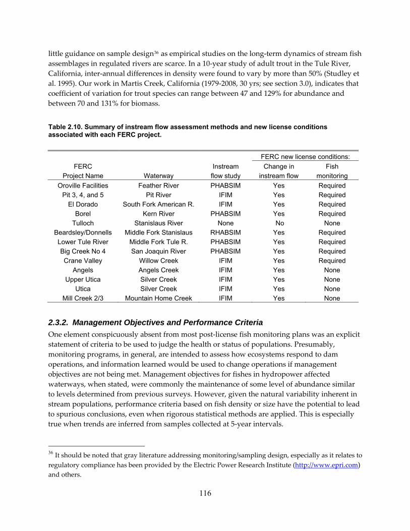
little guidance on sample design36 as empirical studies on the long‐term dynamics of stream fish assemblages in regulated rivers are scarce. In a 10‐year study of adult trout in the Tule River, California, inter‐annual differences in density were found to vary by more than 50% (Studley et al. 1995). Our work in Martis Creek, California (1979‐2008, 30 yrs; see section 3.0), indicates that coefficient of variation for trout species can range between 47 and 129% for abundance and between 70 and 131% for biomass.

Table 2.10. Summary of instream flow assessment methods and new license conditions associated with each FERC project.

FERC new license conditions: FERC Instream Change in Fish

Project Name Waterway flow study instream flow monitoring Oroville Facilities Feather River PHABSIM Yes Required

Pit 3, 4, and 5 Pit River IFIM Yes Required El Dorado South Fork American R. IFIM Yes Required

Borel Kern River PHABSIM Yes Required Tulloch Stanislaus River None No None

Beardsley/Donnells Middle Fork Stanislaus RHABSIM Yes Required Lower Tule River Middle Fork Tule R. PHABSIM Yes Required Big Creek No 4 San Joaquin River PHABSIM Yes Required Crane Valley Willow Creek IFIM Yes Required

Angels Angels Creek IFIM Yes None Upper Utica Silver Creek IFIM Yes None

Utica Silver Creek IFIM Yes None Mill Creek 2/3 Mountain Home Creek IFIM Yes None

2.3.2. Management Objectives and Performance Criteria One element conspicuously absent from most post‐license fish monitoring plans was an explicit statement of criteria to be used to judge the health or status of populations. Presumably, monitoring programs, in general, are intended to assess how ecosystems respond to dam operations, and information learned would be used to change operations if management objectives are not being met. Management objectives for fishes in hydropower affected waterways, when stated, were commonly the maintenance of some level of abundance similar to levels determined from previous surveys. However, given the natural variability inherent in stream populations, performance criteria based on fish density or size have the potential to lead to spurious conclusions, even when rigorous statistical methods are applied. This is especially true when trends are inferred from samples collected at 5‐year intervals.

36 It should be noted that gray literature addressing monitoring/sampling design, especially as it relates to regulatory compliance has been provided by the Electric Power Research Institute (http://www.epri.com) and others.

116

http://www.epri.com/

Table 2.11. Summary of frequency of fisheries monitoring required in new FERC licenses.

FERC License Required fisheries Total No. of Project Name term (yrs) sampling schedule (years) sampling yrs Oroville Facilities TDB Annually (anticipated)

TBD

Pit 3, 4, and 5 40 2011, 2012, 2013, 2014, 2015, 2020, 2025, 2030, 2035, 2041

10

El Dorado 40 2011, 2012, 2016, 2017, 2021, 2022, 2026, 2027, 2031, 2032, 2036, 2037

12

Borel 40 2011, 2016, 2021, 2026, 2031, 2035, 2041, 2046

8

Beardsley/Donnells 40 2007

1

Lower Tule River 30 2007, 2012, 2017, 2022, 2027, 2032

6

Big Creek No. 4 36 2007, 2008, 2009, 2010, 2011, …TBD

5+

Crane Valley 40 2007, 2012, 2017, 2022, 2027, 2032, 2037, 2042

8

Maintaining fish in good condition

A scientifically robust and unambiguous measure of fish health and performance is the concept of maintaining fish in good condition. The term is derived from California Fish and Game Code Section 5937 and states, in part, that:

The owner of any dam shall allow sufficient water at all times to pass through a fishway, or in the absence of a fishway, allow sufficient water to pass over, around or through the dam, to keep in good condition any fish that may be planted or exist below the dam.

Good condition was subsequently defined by Moyle et al. (1998) to encompass characteristics at three levels of biological organization:

1. Individual level: robust body; free of disease, parasite and lesions; reasonable growth rates; and exhibit appropriate behavioral patterns.

2. Population level: multiple age classes (indicating that periodic successful reproduction is occurring); viable population size (adequate numbers to maintain a self‐sustaining population and the long‐term persistence of the population); and healthy individuals.

117

3. Community level: dominated (in terms of abundance or biomass) by co‐evolved native species; predictable structure (limited niche overlap and trophic levels); is resilient in response to stochastic events; is replicated geographically.

This definition was utilized as the foundation for two of the monitoring programs examined: Lower Tule River Project (FERC No. 372; see section 2.2.7) and Big Creek No. 4 Hydroelectric Project, (FERC No. 2017; see section 2.2.8). In the case of the latter project, good condition was used as a performance standard nested in an adaptive management framework to assess the effects of managed spills and scheduled releases on native aquatic species. The final Adaptive Management Plan (SCE 2008) presented a series of decision flow charts which illustrated the incorporation of good condition criteria to assess the effects of hydropower operations (see Figure 2.1)

We believe this approach utilizes a scientifically defensible framework for the protection, mitigation, and enhancement of fish populations and assemblages that deserves wider application in FERC licensing. While annual sampling of fish and other aquatic resources provides the most accurate assessment of trends (see sections 3.0 and 4.0), we acknowledge that such a monitoring program may be overly intensive and impracticable for most hydroelectric projects. Maintaining fish in good condition is an unambiguous performance criterion that protects against misinterpreting trends due to natural variability in populations and provides ecologically meaningful feedback on the effects of hydropower operation.

118

Figure 2.1. Big Creek No. 4 Hydroelectric Project decision pathways for flow modifications (Source: figure 4-1 in SCE 2008).

119

3.0 Factors Affecting the Fish Assemblage in a Sierra Nevada, California, Stream Joseph D. Kiernan1 and Peter B. Moyle2, Center for Watershed Sciences, University of California, One Shields Avenue, Davis, CA 95616. 1 [email protected] 2 [email protected]

Abstract The fishes of Martis Creek, in the Sierra Nevada of California, were sampled at 4 sites annually for 30 yrs, 1979‐2008. This long‐term data set was used to examine the hypotheses that (1) the fish assemblage is persistent and resilient through time, (2) native and alien fishes respond differently to the flow regime, and (3) the principal determinant of fish assemblage composition is flow regime. Annual changes in fish density and biomass were related to 14 attributes of the flow regime, as well as to 13 habitat variables. Despite high inter‐annual variability in mean and peak discharge values, the basic character of flow regime did not change over the period of study. Fish assemblages were persistent at all sample sites but had marked inter‐annual variability in density and biomass. Most native fishes declined while most alien species showed no trends. Only alien rainbow trout increased in both density and biomass at all sites over time. Abundances of native species were tied mostly to habitat variables, while alien species responded to flow magnitude and timing/duration, especially brown trout. Frequency of high‐flow events had a negative relationship with proportion of alien species. While the basic fish assemblage has persisted (despite frequent invasions), assemblage structure appears to be largely the result of density independent processes. Our results indicate the need for continuous annual monitoring of streams with altered flow regimes, as well as to have monitoring of relatively unaltered streams for comparison. Apparent successes or failures in stream management may appear in a different light under long‐term study.

3.1. Introduction Ecologists have long sought to understand processes that affect persistence of populations and communities over time. There is an especially rich history of debate over mechanisms that determine the structure and dynamics of stream fish assemblages (Matthews 1998). Most disagreement has centered on the relative importance of density‐dependent versus density‐independent processes in structuring fish communities. Density‐dependent mechanisms, mainly competition, predation, parasitism and disease, regulate populations via reductions in growth, reproductive output, or survivorship. Density‐dependent regulation has been widely documented in streams (e.g., Elliott 1994, Jenkins et al. 1999, Lobon‐Cervia 2007) and hypothesized to be the only force capable of producing populations with long‐term stability (May 1976, Grossman et al. 1990, Murdoch 1994). Conversely, density‐independent mechanisms such as floods (Erman et al. 1988, Matthews 1998) and drought (Matthews and Marsh‐Matthews 2003, Bêche et al. 2009) affect fish populations via direct mortality or enhanced survivorship during periods of favorable conditions.

Streamflow has been deemed a ‘master variable’ (Poff and Ward 1989, Power et al. 1995) because it influences many physical factors (e.g., water depth, current velocity, and substrate) and ecological interactions (e.g., competition and predation) that limit distribution and

120

mailto:[email protected]


abundance of stream biota. Moreover, a natural flow regime (Poff et al. 1997) is hypothesized to maintain native fish assemblages where life histories are synchronized with the dynamics of a local flow regime (e.g., timing and magnitude). Conversely, the lack of persistence of alien (non‐native) fishes may be caused by their inability to cope with hydrologic conditions that differ from those to which they are adapted (Moyle and Light 1996, Fausch et al. 2001). However, our ability to test these hypotheses and make robust assessments of stability and persistence in populations with generation times exceeding one year is limited by a paucity of long‐term data. Long‐term discharge data are available for many North American streams, quantitative records of fish assemblage composition, especially those collected with comparable sampling effort, are extremely rare (but see studies in Matthews 1998) while short‐term studies often fail to capture the full range of hydrologic variability potentially experienced by fishes and may provide a spurious or incomplete picture of the importance of hydrologic disturbance to assemblage structure. For example, in a five year study (1979‐1984) of Martis Creek, California, Moyle and Vondracek (1985) concluded that, despite inter‐annual variability in streamflow, fish assemblages were persistent largely due to density‐dependent mechanisms (e.g., segregation of species by habitat, microhabitat and diet). However, Strange et al. (1992) analyzed 10 years of data from the same stream and concluded that a pair of very large flood events precipitated a significant shift in the fish assemblage from dominance by native species to dominance by alien species.

Here we expand upon previous studies of Martis Creek and examine variability of the fish assemblage over 30 years (1979‐2008). The extended temporal perspective and range of hydrologic conditions encompassed by our study, including intense floods (1983, 1995, and 2006) and drought (1987‐1992), allowed us to assess the effect of hydrologic variability on population trends and assemblage structure across many generations of the constituent species. Our aim is to re‐test hypotheses posed in Moyle and Vondracek (1985) and Strange et al. (1992). Specifically, (1) the fish assemblage is persistent and resilient through time, (2) native and alien fishes respond differently to the flow regime, especially to floods and drought, and (3) the principal determinant of fish assemblage composition is the flow regime. The latter question is particularly important because of the need to determine fish‐friendly flow regimes in streams with flows regulated by dams (Moyle and Mount 2007, Poff and Zimmerman 2010).

3.2. Methods 3.2.1. Study Site This study was conducted in Martis Creek, a tributary of the Truckee River in Nevada and Placer Counties, California, USA (39°19’ N, 120°07’ W). In 1979, four 40 m stream reaches were selected as representative of typical habitats in the creek and established as permanent sample sites. The sites were distributed along a 2.9 km segment bounded upstream by Martis Dam (elevation 1745 m) and downstream by a high gradient riffle cascade. The four sample sites (hereafter S1, S2, S3, and S4) were located 0.1, 0.3, 1.2, and 2.4 km above the confluence with the Truckee River, respectively. The climate is cool‐summer Mediterranean and precipitation generally falls as snow or mixed snow and rain between October and May. Peaks in the annual hydrograph are produced by rain on snow events and spring snowmelt. Peak flows generally

121

occur between January and early June and low (base) flows between August and November (Fig. 3.1). Martis Dam was constructed in 1972 for flood control and impounds 0.28 km2 Martis Creek Reservoir (storage capacity = 1,234 m3). The reservoir was originally designed to spill through a vertical standpipe; however, only temporary flood storage is currently permitted due to chronic seepage and active dam failure. Hence, reservoir outflows generally equal inflows and discharge in the study area mimics the natural flow regime except that extreme high flow events are damped (Moyle and Vondracek 1985, Strange et al. 1992). One‐day maximum discharge prior to dam construction was 50.9 m3/s (1 February 1963; period of record 1959‐1971) compared to 17.3 m3/s (3 January 2006) during the post‐dam era (US Geological Survey [USGS] gage 10339400; http://waterdata.usgs.gov).

Dai

ly d

isch

arge

(m3 /s

)

0

5

10

15

20

O N D J F M A M J SAJ

WINTER

Mea

n m

ax. d

aily

wat

er te

mpe

ratu

re (°

C)

0

5

10

15

20

25

30

Figure 3.1. Mean daily discharge (solid line) and maximum daily water temperature (dotted line) of Martis Creek, California for water years 1979-2008. Gray shaded area represents the minimum and maximum recorded discharge for each day during the 30 years of study. Data are from USGS gage 10339400.

3.2.2. Fish sampling From 1979‐2008 (except 1986) fish populations were surveyed once annually in August or September during low flow conditions. On each occasion, sample sites were isolated with block nets and fish were collected using a backpack electrofisher. Three‐pass removal sampling was conducted during most visits (92%); however, single or two‐pass sampling was occasionally employed due to equipment failures. Captured fish were identified to species and measured for standard length (± 1.0 mm). Biomass was determined by water displacement or by weighing

122

with a Pesola spring scale (± 1.0 g; Pesola AG, Baar, Switzerland). In some cases masses were estimated from taxon‐specific length weight regression equations (P.B. Moyle, unpublished data). Population estimates for each species were derived by maximum‐likelihood estimation using MicroFish version 3.0 (Van Deventer and Platts 1989). Abundance and biomass totals were divided by the area sampled to generate annual estimates of species density (individuals/100 m2) and biomass (kg/100 m2) at each site. In most years, the majority of fish were young‐of‐year, so high abundance would reflect successful spawning in the fall or spring prior to sampling.

3.2.3. Habitat variables Thirteen habitat variables were measured or estimated at each site each year. Variables included: reach length, mean wetted width, mean depth, maximum depth, percentage riffle, run, and pool habitat, percentage canopy cover, and substrate composition. Wetted stream width and three depth measurements (± 1.0 cm, measured at 25%, 50%, and 75% wetted width) were quantified at 10 evenly spaced transects along the length of each sample site. Maximum depth was the deepest point in the entire sample reach. Substrate composition was visually estimated to the nearest 5% as sand/silt (<2 mm), gravel (2‐64 mm), cobble (>64‐256 mm), or boulder (>256 mm). Beginning in 1990, the proportion of stream habitat containing different forms of aquatic vegetation (i.e., emergent, submerged, floating mats, and filamentous algae) was also visually estimated (± 5%; Table 3.1).

3.2.4. Stream water temperature and hydrologic attributes Stream discharge and water temperature data were obtained from USGS gaging station 10339400 located 0.3 km downstream of Martis Creek Dam. We calculated mean weekly maximum stream temperature (i.e., 7‐day running averages; MWMT) for each day of the year and summed the number of days MWMT ≥ 20°C annually. A MWMT threshold of 20°C was chosen because it represents a sub‐lethal level above which Paiute sculpin, the most thermally intolerant species of the native fish assemblage, become increasingly rare (Moyle 2002). Mean daily discharge data representing the complete period of record (water years 1974‐2008) were used to determine median annual stream flow (0.55 m3/s). Each study year was then classified as one of three water‐year types based on mean annual flow: normal, wet (≥ 1.15 m3/s [75th percentile]) or dry (≤ 0.33 m3/s [25th percentile]). Discharge data were unavailable for the period 1991‐1993 and attempts to develop regression based estimates of daily flow using gaging stations in nearby basins were unsuccessful. However, we were able to derive estimates of mean annual flow (Qmaf, [m3/s]) using data for nearby Sagehen Creek (Nevada County, California; USGS gage 10343500). The relationship between Qmaf in the two basins was described by the equation:

Log10 Qmaf Martis = 0.32 + 0.95 × Log10 Qmaf Sagehen (r2 = 0.98, F1,32 = 1517.98, P <0.001).

123

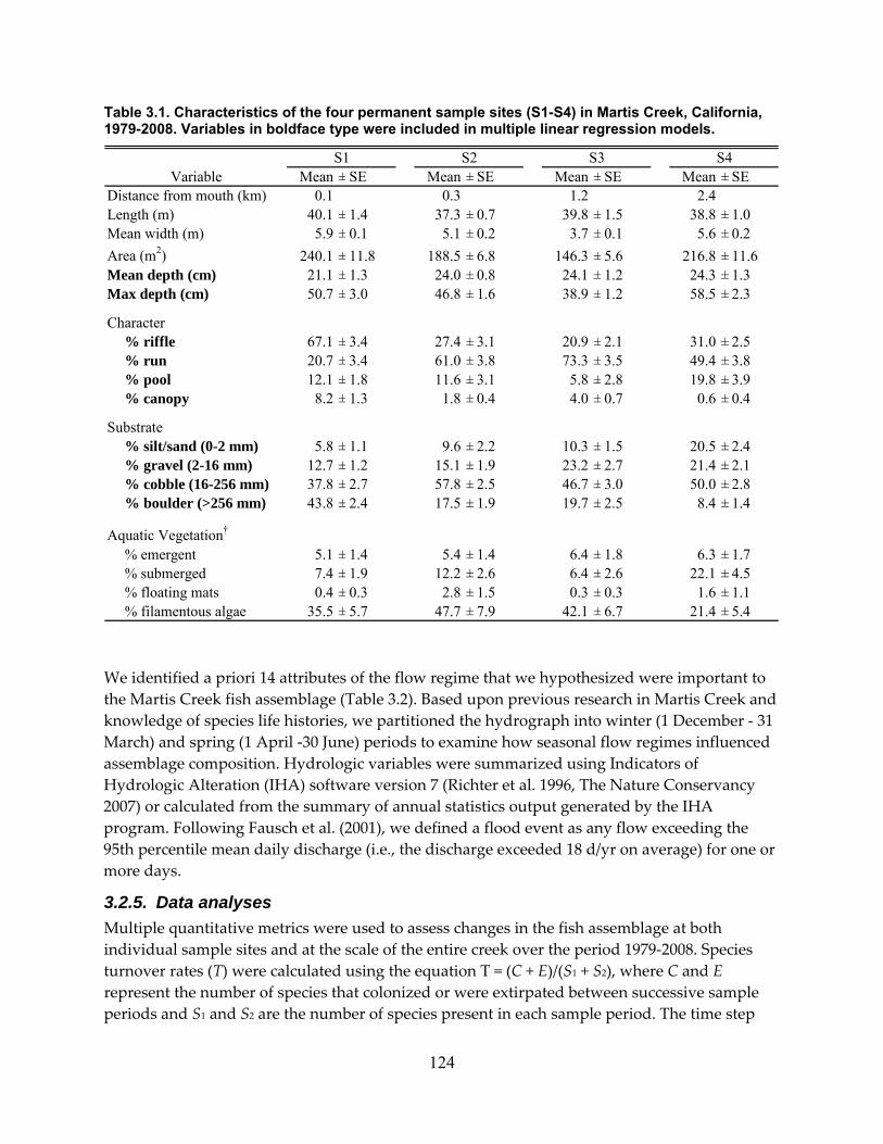
Table 3.1. Characteristics of the four permanent sample sites (S1-S4) in Martis Creek, California, 1979-2008. Variables in boldface type were included in multiple linear regression models.

Mean ± SE Mean ± SE Mean ± SE Mean ± SEDistance from mouth (km) 0.1 0.3 1.2 2.4Length (m) 40.1 ± 1.4 37.3 ± 0.7 39.8 ± 1.5 38.8 ± 1.0Mean width (m) 5.9 ± 0.1 5.1 ± 0.2 3.7 ± 0.1 5.6 ± 0.2Area (m2) 240.1 ± 11.8 188.5 ± 6.8 146.3 ± 5.6 216.8 ± 11.6Mean depth (cm) 21.1 ± 1.3 24.0 ± 0.8 24.1 ± 1.2 24.3 ± 1.3Max depth (cm) 50.7 ± 3.0 46.8 ± 1.6 38.9 ± 1.2 58.5 ± 2.3

Character% riffle 67.1 ± 3.4 27.4 ± 3.1 20.9 ± 2.1 31.0 ± 2.5% run 20.7 ± 3.4 61.0 ± 3.8 73.3 ± 3.5 49.4 ± 3.8% pool 12.1 ± 1.8 11.6 ± 3.1 5.8 ± 2.8 19.8 ± 3.9% canopy 8.2 ± 1.3 1.8 ± 0.4 4.0 ± 0.7 0.6 ± 0.4

Substrate% silt/sand (0-2 mm) 5.8 ± 1.1 9.6 ± 2.2 10.3 ± 1.5 20.5 ± 2.4% gravel (2-16 mm) 12.7 ± 1.2 15.1 ± 1.9 23.2 ± 2.7 21.4 ± 2.1% cobble (16-256 mm) 37.8 ± 2.7 57.8 ± 2.5 46.7 ± 3.0 50.0 ± 2.8% boulder (>256 mm) 43.8 ± 2.4 17.5 ± 1.9 19.7 ± 2.5 8.4 ± 1.4

Aquatic Vegetation†

% emergent 5.1 ± 1.4 5.4 ± 1.4 6.4 ± 1.8 6.3 ± 1.7% submerged 7.4 ± 1.9 12.2 ± 2.6 6.4 ± 2.6 22.1 ± 4.5% floating mats 0.4 ± 0.3 2.8 ± 1.5 0.3 ± 0.3 1.6 ± 1.1% filamentous algae 35.5 ± 5.7 47.7 ± 7.9 42.1 ± 6.7 21.4 ± 5.4

VariableS4S1 S2 S3

We identified a priori 14 attributes of the flow regime that we hypothesized were important to the Martis Creek fish assemblage (Table 3.2). Based upon previous research in Martis Creek and knowledge of species life histories, we partitioned the hydrograph into winter (1 December ‐ 31 March) and spring (1 April ‐30 June) periods to examine how seasonal flow regimes influenced assemblage composition. Hydrologic variables were summarized using Indicators of Hydrologic Alteration (IHA) software version 7 (Richter et al. 1996, The Nature Conservancy 2007) or calculated from the summary of annual statistics output generated by the IHA program. Following Fausch et al. (2001), we defined a flood event as any flow exceeding the 95th percentile mean daily discharge (i.e., the discharge exceeded 18 d/yr on average) for one or more days.

3.2.5. Data analyses Multiple quantitative metrics were used to assess changes in the fish assemblage at both individual sample sites and at the scale of the entire creek over the period 1979‐2008. Species turnover rates (T) were calculated using the equation T = (C + E)/(S1 + S2), where C and E represent the number of species that colonized or were extirpated between successive sample periods and S1 and S2 are the number of species present in each sample period. The time step

124

between most sample periods was one year, but turnover for 1987 was relative to 1985 population estimates. Turnover rates were averaged across all years and an index of overall persistence was calculated as 1 – mean T (Meffe and Minckley 1987). Persistence indicates whether the same species are present over time and index values range from zero (no persistence) to one (complete persistence).

Table 3.2. Hydrological variables used to predict annual fish densities in Martis Creek, California, 1979-2008. Predicted effects on native and alien species are classified as positive (+), weakly positive (0+), neutral (0), weakly negative (0–), negative (–), or strongly negative (– –).

Predicted effect of higher values on: Hydrologic variable Native Fish Alien Fish Magnitude 1) Mean annual discharge 0+ – – 2) Mean winter discharge + – – 3) Maximum winter discharge 0– – – 4) Mean spring discharge 0– – 5) Maximum spring discharge – – – Duration 6) Mean of the 7 consecutive days 0– – – of highest annual discharge 7) Mean of the 7 consecutive days – – 0– of lowest annual discharge 8) Mean duration of winter floods (days) 0+ – – 9) Mean duration of spring floods (days) – – – Frequency 10) Number of winter floods ≥ 1 day 0+ – – duration per year 11) Number of spring floods ≥ 1 day – – – – duration per year

Timing 12) Ordinal date of annual min. discharge 0– 0+ 13) Ordinal date of spring max. discharge 0– 0+ 14) Ordinal date of winter max. discharge 0– 0+

To quantify among year variability in abundance and biomass we calculated coefficients of variation (CV, expressed as a percentage) for each species. Following Freeman et al. (1988), populations were classified as: (1) highly stable (CV ≤ 25%), (2) moderately stable (25% < CV ≤ 50%), (3) moderately fluctuating (50% < CV ≤ 75%), and (4) highly‐fluctuating (CV > 76%). Site‐specific temporal trends in species abundance and biomass were assessed using nonparametric Spearman’s rank correlation coefficients (rs) with a Type I error rate (α) of 0.05. To determine overall population trends (i.e., data pooled across all sites), we created log‐linear Poisson regression models with adjustments for overdispersion and serial correlation using the program

125

TRIM (Trends and Indices for Monitoring Data; Pannekoek and van Strien 1996). Annual density estimates for each species were converted to indices of abundance using 1979 as the base year. The stepwise selection procedure within TRIM was then used to identify change points based on significant changes in slope (Wald tests with a significance‐level threshold value of 0.05).

We used time‐lag regression analysis (Collins et al. 2000) to determine whether fish assemblages at each site had undergone directional change. Separate species × year data matrices containing fourth‐root transformed densities were created for each sample site. Bray‐Curtis distances were calculated for each possible pair of sample dates (years) and regressed against the square root of the time lag between each observation for all possible lags (i.e., 1 – 29 yrs). This technique produces a measure of stability with three potential outcomes: (1) a regression line with a slope not significantly different from zero indicates either assemblage stability (constancy) or complete stochastic variability, (2) a significant, positive linear regression indicates an assemblage undergoing directional change, and (3) a significant, linear, and negative slope indicates an unstable assemblage converging on a structure characteristic of an earlier time period (Collins et al. 2000). Detrended correspondence analysis (DCA) was then used to assess temporal change in ordination space across time. Ordinations were performed in PC‐ORD 5 (MjM Software, Gleneden Beach, OR, USA).

We used stepwise multiple regressions to examine the relationship between environmental variables and the density of each species. Due to a high degree of collinearity among the 14 flow attributes (Table 3.2), principal component analysis (PCA) was applied to the correlation matrix of these variables. Two ecologically interpretable axes (eigenvalues >1.0) were retained and subsequently included with 10 habitat variables (Table 3.1) in initial regression models. To examine the potential effects of brown trout predation on each species, a second model was created which included brown trout density as an additional independent variable. Multiple regressions were performed using NCSS version 2004 (NCSS, Kaysville, UT, USA). Criteria for entering and removing variables from the multiple regression models was set at P = 0.05 and P = 0.10, respectively. Spearman’s rank correlation coefficients were used to examine the relationships between mean annual discharge, one day maximum discharge, and the proportion of the total fish assemble comprised of alien fishes. Lastly, the relationship between seasonal flood frequency and proportion of alien fishes was assessed using a generalized linear model with quasi‐Poisson error distribution to correct for overdispersion, using R version 2.11 (R Foundation for Statistical Computing, Vienna, Austria).

3.3. Results 3.3.1. Hydrologic attributes Despite high inter‐annual variability in mean and peak discharge values (Fig. 3.2), the long‐term character of the Martis Creek hydrograph did not change between 1979 and 2008. Of the 33 hydrologic variables calculated by the IHA program, only low pulse duration (i.e., periods within a year when daily flows were in the lower 25th percentile based on complete period of record) exhibited a statistically significant negative trend over time (slope = ‐2.49, F1,27 = 10.61, P < 0.01, r2 = 0.34; Table 3.3).

126

1980 1985 1990 1995 2000 2005

Mea

n an

nual

dis

char

ge (m

3 /s)

0.0

0.5

1.0

1.5

2.0

Water year

Pea

k in

stan

tane

ous

disc

harg

e (m

3 /s)

0.1

1

10

100

Wet yearNormal year Dry year

Figure 3.2. Annual mean (bars) and peak instantaneous (diamonds) discharge during each water year of study (1979-2008). The horizontal dash line represents median discharge for the complete period of record (1974-2008; USGS gage 10339400). Gray, hatched, and black vertical bars indicate wet (≥ 75th percentile), normal, and dry (≤ 25th percentile) water year types, respectively. Note log scale for instantaneous discharge.

3.3.2. Community composition Collectively the four sample sites supported 14 species of fish over the period of study (Table 3.4). Only three species occurred during all years: native Paiute sculpin and alien brown trout and rainbow trout. Native Tahoe sucker were captured during every year except 1999. No species was found at all four sample sites across every year of study. Mean (± SE) species richness was greatest at the upstream‐most site (S4, 5.6 ± 0.2 species; N = 29) and lowest at S3 (3.8 ± 0.3 species; N = 29). Annual species richness ranged from 1 to 8 species at individual sample sites (Appendix C) and from 5 to 10 at the scale of the entire creek (pooled across all sites). Five species were rare in terms of abundance or frequency of occurrence (< 25% of yrs) and are not classified as resident populations: Lahontan cutthroat trout (N = 6 yrs), Lahontan tui chub (N = 2 yrs), bluegill (N = 2 yrs), brook trout (N = 2 yrs), and largemouth bass (N = 2 yrs). Of these species, brook trout and tui chub presumably moved up from the Truckee River and cutthroat trout originated from artificially maintained populations upstream in Martis Creek Reservoir and downstream in the Truckee River. Largemouth bass and bluegill are recent invaders that first occurred at the downstream‐most site (S1) in 2003 and 2004, respectively.

127

Table 3.3. Results of the Indicators of Hydrologic Alteration analysis for Martis Creek, California, 1979-2008. Values are derived from non-parametric regressions of hydrologic variables against time.

IHA Group Slope r2 F P1. Magnitude of monthly conditions

October -0.002 0.02 0.60 0.500November -0.008 0.06 1.92 0.250December -0.006 0.03 0.73 0.500January 0.006 0.00 0.09 0.500February -0.021 0.08 2.59 0.250March -0.008 0.01 0.24 0.500April 0.005 0.00 0.06 0.500May -0.008 0.00 0.07 0.500June -0.031 0.07 2.00 0.250July -0.012 0.05 1.55 0.250August -0.002 0.03 0.81 0.500September -0.003 0.04 1.27 0.500

2. Magnitude and duration of monthly extremes1-day minimum -0.001 0.02 0.45 0.5003-day minimum -0.001 0.00 0.13 0.5007-day minimum 0.000 0.00 0.06 0.50030-day minimum -0.001 0.01 0.29 0.50090-day minimum -0.003 0.04 1.11 0.5001-day maximum -0.170 0.08 2.29 0.2503-day maximum -0.110 0.04 1.17 0.5007-day maximum -0.078 0.03 0.88 0.50030-day maximum -0.044 0.03 0.92 0.50090-day maximum -0.016 0.01 0.41 0.500Number of zero days 0.000 0.00 0.00 0.500Base flow index 0.001 0.00 0.11 0.500

3. Timing of annual extremesDate of minimum -0.061 0.00 0.00 0.500Date of maximum -1.431 0.02 0.58 0.500

4. Frequency and duration of high and low pulseLow pulse count 0.099 0.16 5.24 0.050Low pulse duration -2.493 0.34 10.61 0.005High pulse count -0.014 0.00 0.09 0.500High pulse duration 0.119 0.00 0.09 0.500

5. Rate and frequency of water changesRise rate -0.001 0.06 1.73 0.250Fall rate 0.001 0.13 4.31 0.050Number of reversals 0.402 0.03 0.96 0.500

128

Table 3.4. Frequency of occurrence of fish species during annual surveys of four permanent sample sites (S) in Martis Creek, California, 1979-2008. The ‘all’ sites category indicates the number of years a species was found at all sample sites.

NativeLahontan cutthroat trout (Oncorhynchus clarki henshaw 3 2 1 1 0Lahontan redside (Richardsonius egregius ) 2 1 4 13 0Speckled dace (Rhinichthys osculus ) 2 4 10 25 0Lahontan tui chub (Siphateles bicolor ) 0 1 0 1 1Mountain sucker (Catostomus platyrhynchus ) 3 7 6 16 0Mountain whitefish (Prosopium williamsoni ) 10 1 0 0 0Paiute sculpin (Cottus beldingi ) 28 27 19 18 14Tahoe sucker (Catostomus tahoensis ) 7 14 17 28 6

AlienBluegill (Lepomis macrochirus ) 2 0 0 0 0Brook trout (Salvelinus fontinalis ) 2 0 0 0 0Brown trout (Salmo trutta ) 29 28 27 26 25Green sunfish (Lepomis cyanellus ) 0 1 3 12 0Largemouth bass (Micropterus salmoides ) 3 2 1 1 0Rainbow trout (Oncorhynchus mykiss ) 29 28 23 22 19

SpeciesS2 S3 S4S1

(N =29) (N =28) (N =29) (N =29)All

(N =29)

3.3.3. Temporal changes in assemblage structure Fish assemblages were moderately persistent (1 T− ≥ 0.74) at all sample sites (Appendix C) but exhibited marked inter‐annual variability in density and biomass (Fig. 3.3). Overall, the highest mean annual estimates (pooled across sample sites) of total fish density (499 ± 242 individuals/100 m2) and biomass (2.4 ± 0.4 kg/100 m2) occurred in 1981 (Fig. 3.4). Conversely, the lowest mean estimates of total density and biomass were recorded in 1991 (27 ± 10 individuals/100m2) and 1983 (0.4 ± 0.1 kg/100 m2), respectively. During the initial years of study (i.e., 1979‐1982) fish assemblages were dominated by native species. Mean proportion of native fish peaked in 1980 (92 ± 6% of total density and 67 ± 20% of total biomass) then abruptly declined until 1988 (2 ± 2% of total density, 2 ± 1% of total biomass; Fig. 3.4). While the proportion of native fishes subsequently rebounded between 1989 and 1994, it never recovered to previous levels (e.g., 1981; Fig 3.4).

129

0

20

40

60

80

100

19801990

2000

1 2 3 4

Rel

ativ

e ab

unda

nce

(%) A) Brown trout

0

20

40

60

80

100

19801990

2000

1 2 3 4

B) Rainbow trout

0

20

40

60

80

100

19801990

2000

1 2 3 4

Rel

ativ

e ab

unda

nce

(%) D) Paiute sculpin

0

20

40

60

80

100

19801990

2000

1 2 3 4

E) Tahoe sucker

0

20

40

60

80

100

19801990

2000

1 2 3 4 Year

F) Mountain sucker

0

20

40

60

80

100

19801990

2000

1 2 3 4

Rel

ativ

e ab

unda

nce

(%)

Sample Site

G) Speckled dace

0

20

40

60

80

100

19801990

2000

1 2 3 4Sample Site

H) Lahontan redside

0

20

40

60

80

100

19801990

2000

1 2 3 4

Year

Sample Site

I) Mountain whitefish

0

20

40

60

80

100

19801990

2000

1 2 3 4 Year

C) Green sunfish

Figure 3.3. Relative abundances of key fish species during annual surveys of four permanent sample sites in Martis Creek, California, 1979-2008. Alien fish are represented in plots A-C while native fish are represented in plots D-I. Sample sites 1 and 4 represent the downstream-most and upstream-most locations, respectively (see methods).

3.3.4. Population trends Most native fish populations showed trends of declining abundance over the period of study (Fig. 3.3; Table 3.5). Only Paiute sculpin at sites S3 and S4 demonstrated statistically significant increases in density and/or biomass (Table 3.5). Temporal trends for alien species were inconsistent among sample sites. Rainbow trout were the only alien species to exhibit increases in both density and biomass at all sites over time (Table 3.5).

The identification of change points on individual species abundance indices highlighted a marked lack of synchrony in the timing of population changes among taxa (Table 3.6). The Tahoe sucker population exhibited the greatest number of significant changes among the native

130

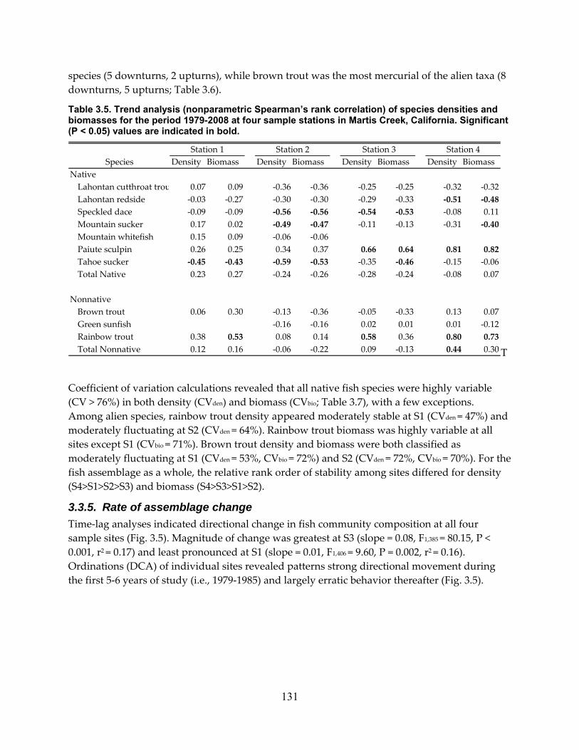
species (5 downturns, 2 upturns), while brown trout was the most mercurial of the alien taxa (8 downturns, 5 upturns; Table 3.6).

Table 3.5. Trend analysis (nonparametric Spearman’s rank correlation) of species densities and biomasses for the period 1979-2008 at four sample stations in Martis Creek, California. Significant (P < 0.05) values are indicated in bold.

Density Biomass Density Biomass Density Biomass Density Biomass NativeLahontan cutthroat trou 0.07 0.09 ‐0.36 ‐0.36 ‐0.25 ‐0.25 ‐0.32 ‐0.32Lahontan redside ‐0.03 ‐0.27 ‐0.30 ‐0.30 ‐0.29 ‐0.33 ‐0.51 ‐0.48Speckled dace ‐0.09 ‐0.09 ‐0.56 ‐0.56 ‐0.54 ‐0.53 ‐0.08 0.11Mountain sucker 0.17 0.02 ‐0.49 ‐0.47 ‐0.11 ‐0.13 ‐0.31 ‐0.40Mountain whitefish 0.15 0.09 ‐0.06 ‐0.06Paiute sculpin 0.26 0.25 0.34 0.37 0.66 0.64 0.81 0.82Tahoe sucker ‐0.45 ‐0.43 ‐0.59 ‐0.53 ‐0.35 ‐0.46 ‐0.15 ‐0.06Total Native 0.23 0.27 ‐0.24 ‐0.26 ‐0.28 ‐0.24 ‐0.08 0.07

NonnativeBrown trout 0.06 0.30 ‐0.13 ‐0.36 ‐0.05 ‐0.33 0.13 0.07Green sunfish ‐0.16 ‐0.16 0.02 0.01 0.01 ‐0.12Rainbow trout 0.38 0.53 0.08 0.14 0.58 0.36 0.80 0.73Total Nonnative 0.12 0.16 ‐0.06 ‐0.22 0.09 ‐0.13 0.44 0.30

SpeciesStation 1 Station 3 Station 4Station 2

T

Coefficient of variation calculations revealed that all native fish species were highly variable (CV > 76%) in both density (CVden) and biomass (CVbio; Table 3.7), with a few exceptions. Among alien species, rainbow trout density appeared moderately stable at S1 (CVden = 47%) and moderately fluctuating at S2 (CVden = 64%). Rainbow trout biomass was highly variable at all sites except S1 (CVbio = 71%). Brown trout density and biomass were both classified as moderately fluctuating at S1 (CVden = 53%, CVbio = 72%) and S2 (CVden = 72%, CVbio = 70%). For the fish assemblage as a whole, the relative rank order of stability among sites differed for density (S4>S1>S2>S3) and biomass (S4>S3>S1>S2).

3.3.5. Rate of assemblage change Time‐lag analyses indicated directional change in fish community composition at all four sample sites (Fig. 3.5). Magnitude of change was greatest at S3 (slope = 0.08, F1,385 = 80.15, P < 0.001, r2 = 0.17) and least pronounced at S1 (slope = 0.01, F1,406 = 9.60, P = 0.002, r2 = 0.16). Ordinations (DCA) of individual sites revealed patterns strong directional movement during the first 5‐6 years of study (i.e., 1979‐1985) and largely erratic behavior thereafter (Fig. 3.5).

131

Table 3.6. Statistically significant change points derived from indexed annual species abundances, 1979-2008. Solid circles indicate significant downturns in the population trajectory and open circles indicate significant upturns. Water year type (WYT) designations are dry (D), normal (N), and wet (W); see methods section for definitions.

1979

1980

1981

1982

1983

1984

1985

1986

1987

1988

1989

1990

1991

1992

1993

1994

1995

1996

1997

1998

1999

2000

2001

2002

2003

2004

2005

2006

2007

2008

Species WYT = N N D W W W N W N D N D D D N D W N W N W N D N N N N W D N

● ○ ● ○● ○ ● ○ ●

○ ● ○ ●● ● ○ ●

○ ● ○○ ● ● ○ ● ● ●

● ○ ● ○ ● ○ ● ● ○ ● ● ○ ●● ● ○○ ● ● ○ ●

NativeLahontan redsideMountain suckerMountain whitefishPaiute sculpinSpeckled dace

Rainbow troutGreen sunfish

Tahoe sucker

Alien (non‐native)Brown trout

Table 3.7. Coefficients of variation (%) of species density and biomass at each sample site in Martis Creek, California, 1979-2008.

Density Biomass Density Biomass Density Biomass Density Biomass NativeLahontan redside 452 539 529 529 496 419 334 269Speckled dace 403 375 347 467 223 308 81 153Mountain sucker 365 452 329 289 299 261 197 206Mountain whitefish 227 338 529 529Paiute sculpin 88 106 98 122 176 197 180 232Tahoe sucker 205 289 176 192 154 188 90 132

AlienBrown trout 53 72 72 70 80 84 126 88Green sunfish 529 529 383 456 173 175Rainbow trout 47 71 64 82 112 114 129 131

Station 4Species

Station 1 Station 2 Station 3

132

Year

1979

1980

1981

1982

1983

1984

1985

1986

1987

1988

1989

1990

1991

1992

1993

1994

1995

1996

1997

1998

1999

2000

2001

2002

2003

2004

2005

2006

2007

2008

Prop

ortio

n to

tal b

iom

ass

0 .0

0.2

0.4

0.6

0.8

1.0

Bio

mas

s (k

g/10

0 m

2 )

0 .1

1

10

Total Fish Assemblage

Native Fishes

Prop

ortio

n to

tal d

ensi

ty

0 .0

0.2

0.4

0.6

0.8 Native fishes

Den

sity

(in

divi

dual

s/10

0 m

2 )

1

10

100

1000Total Fish Assemblage

Native Fishes

Total Fish Assemblage

(A)

(B)

(C)

(D) Native fishes

Figure 3.4.Time series of density and biomass estimates for the Martis Creek fish assemblage, 1979-2008. Bars (A, C) and circles (B, D) represent the annual mean (± 1 SE) of four sample stations. Black bars are mean values for the complete fish assemblage and gray bars are for native fishes only. No data were collected in 1986. Note log scale for plots A and C.

133

0

20

40

60

80

100

120

Time lag (sqrt years)0 1 2 3 4 5

0.0

0.2

0.4

0.6

0.8

S4 r2 = 0.08, P <0.001

Bra

y-C

urtis

dis

tanc

e

0.0

0.2

0.4

0.6

0.8

0.0

0.2

0.4

0.6

0.8

S2 r2 = 0.10, P <0.0010.0

0.2

0.4

0.6

0.8

1.0

S3 r2 = 0.16, P <0.001

S1 r2= 0.02, P = 0.002 S1

0

20

40

60

80

100

120

01

88

04 00

9002

929193

8584

8783070889

97989903

06

79

80

81

8296

05

94

95

S1

0

20

40

60

80

100

120

93

79

80

8182

83

8485

87

88

89

91

92

94

95

96

9798 99000102

0304

0506

0708

S2

79

80

81

82

83

84

85

87

88

89

90 91

92

93 94

95

96

97989900

0102

03

0405

06

07

08

S3

DCA Axis 10 50 100 150 200 250

0

20

40

60

80

100

120

79

80

8182

83

84

85

87

88

89

9091

92

93

94

95

96

97

98

9900

0203

04

05 06

07

0801

S4

DC

A A

xis

2

Figure 3.5. Time-lag and Bray-Curtis distance of change in fish density (A) and detrended correspondence analysis (DCA) by year (B) for each sample site. Points represent differences in years for all year-to-year combinations plotted against Bray-Curtis distance. Each node in the DCA biplot represents the fish assemblage in a given year. Years are connected by a line to illustrate change over time.

134

3.3.6. Environmental variables and fish densities Principal component analysis of the 14 hydrologic attributes (Table 3.2) produced two interpretable axes (Fig. 3.6). The first PC axis accounted for 63% of the variance in the original data and was related to annual discharge with drier water years in the positive direction. The second PC axis accounted for 11% of the total variance and represented a gradient in timing and duration of high stream flow events. Positive values on the second axis are associated with high flow events earlier in the water year (i.e., winter), whereas negative values indicate late season (spring) spates. Values intermediate (near zero) on the second axis indicate a lack of seasonality stemming from either similar high flows during both seasons (e.g., 1983, 2006) or completely flood‐free water years (e.g., 1981, 2007) (Figs. 3.2 and 3.6).

Principle component 1 (63.4%)-6 -4 -2 0 2 4 6

Prin

cipl

e co

mpo

nent

2 (

11.9

%)

-4

-2

0

2

4

1985

High annual Discharge

Early in year(winter)

1997

1984 1988

1983

1982

1995

20012008

1986

20042006

1980

1999

1996 1998

1979

2005

2000

2003

2007

19811987

19942002

1989

Low annual Discharge

Late in year(spring)

"tim

ing

of p

eak

flow

"

"magnitude" Figure 3.6. Results of the principal component analysis (PCA) performed on the correlation matrix of hydrologic variables presented in Table 3.2. Two ecologically interpretable axes accounting for 75.3% of the original variation were retained and included in multiple linear regression analyses.

Stepwise multiple regression models indicated that abundances of native species were more frequently described by habitat variables than hydrology or temperature (Table 3.8). Only the two native sucker species were significantly influenced by flow with both responding positively to the timing and/or duration of elevated spring flow events (Table 3.8). In contrast, flow variables were significant in modeling the abundance of two of the three alien species in the

135

system (brown trout and green sunfish). Brown trout density was especially influenced by hydrology as both flow magnitude (PC1) and timing/duration (PC2) were significant in the final regression model (Table 3.8).

Table 3.8. Results of stepwise multiple linear regression analysis using species density as the dependent variable. Data were transformed prior to analysis. PC1 and PC2 were derived from principle component analysis of flow attributes. Higher PC1 values can be interpreted as lower annual discharge (dry water years). PC2 relates to seasonality of peak flows with positive values indicating high flow events earlier in the water year (i.e., winter) and negative values indicating late season (spring) spates. A second set of regression models which included brown trout density as a proxy for brown trout predation did not change the results for any species.

Species Independent variable

Standardized coefficient R2 df F P

Native Lahontan redside % boulder -0.32 0.15 2, 112 9.68 <0.001 % pool 0.30 Mountain whitefish % boulder 0.32 0.10 2, 111 6.32 0.003 mean depth -0.24 Mountain sucker % boulder -0.36 0.21 3, 100 8.21 <0.001 % gravel -0.24 PC 2 -0.24 Paiute sculpin % silt/sand -0.30 0.10 1, 112 12.61 0.001 Speckled dace % boulder -0.59 0.30 3, 111 15.54 <0.001 max. depth 0.25 % gravel -0.19 Tahoe sucker % boulder -0.47 0.41 3, 100 22.09 <0.001 PC 2 -0.32 % pool 0.25 Alien Brown trout PC 1 -0.24 0.11 3, 100 4.10 0.009 % gravel -0.19 PC 2 -0.19 Rainbow trout % boulder 0.32 0.17 2, 111 10.89 <0.001 mean depth -0.28 Green sunfish % silt/sand 0.36 0.13 2, 100 7.42 0.001

136

In general, there was an inverse relationship between the proportion of the fish assemblage composed of alien species and mean annual discharge (Fig. 3.7a). One day maximum discharge values in both winter and spring were also negatively correlated with the proportion of alien species (Fig. 3.7b). Additionally, there was a negative relationship between frequency of floods events (i.e., number of flood events ≥ 1 day in duration) and proportion of alien species in both winter and spring, but only the latter season was statistically significant (Fig. 3.7c). Results for the second set of regression models which included brown trout density (a proxy for brown trout predation) in the set of potential independent variables were the same as the first models in all cases indicating brown trout density had no effect on the density of other fish species independently of habitat, water temperature and streamflow variables.

One day max discharge

Log10(m3/s + 1)

0.0 0.5 1.0Mean annual

discharge (m3/s)

0.0 0.5 1.0 1.5 2.0

Prop

ortio

n of

alie

n fis

h

0.0

0.2

0.4

0.6

0.8

1.0 (A) (B) (C)

Frequency of floods (No./season)

0 2 4 6 8 10

rs = -0.47, P = 0.01rs = -0.39, P = 0.03

Winter, P = 0.31Spring, P = 0.04

Winter

Springrs = -0.50, P = 0.01

Figure 3.7. Proportion of alien fish as a function of mean (A) and maximum (B) annual discharge, and frequency of flood events during winter (1 December - 31 March) and spring (1 April - 30 June) of each water year (C). P-values are based on Spearman’s rank correlation (rs) for A and B and a quasi-Poisson regression model for C.

3.4. Discussion 3.4.1. Fish assemblage persistence and resilience Despite a high degree of annual variability in species abundances, the Martis Creek fish assemblage showed considerable persistence and resilience over the 29 years of study, supporting our first hypothesis. Of the seven species originally reported by Moyle and Vondracek (1985) to constitute the fish assemblage (i.e., brown trout, rainbow trout, speckled dace, Lahontan redside, mountain sucker, Tahoe sucker, and Paiute sculpin) all were present during ≥ 1 of the last 5 survey years (2004‐2008). Two additional species, mountain whitefish and green sunfish, were occasionally encountered during the study period, but their densities were generally low and their distributions limited. Mountain whitefish were captured during 35% of annual surveys (N=10) but were mainly restricted to the sample station near the mouth of the creek where stream gradient is high and larger substrates predominate. Only young‐of‐the‐year whitefish were observed during sampling and individuals presumably originated from the Truckee River because adults have never been documented in Martis Creek. Conversely,

137

green sunfish were present in 49% of annual surveys (N=14), but rarely captured below the upstream‐most sample site near the Dam. Green sunfish are abundant in Martis Creek Reservoir and presumably washed into the creek during large rainfall events that cause the reservoir to spill. Although they are potentially predators on small fish (Moyle 2002), their numbers were usually low enough so that it is unlikely they had much affect on the fish assemblages.

3.4.2. Native vs. alien fishes During the initial years of study the fish assemblage was dominated by native species (i.e., Tahoe sucker, Lahontan redside, Paiute sculpin, and speckled dace) with stable relative abundances and trout were relatively uncommon (Moyle and Vondracek 1985). In 1983, low winter stream flows were followed by severe flooding during the spring. This sequence of hydrologic events resulted in relatively high recruitment of brown trout and poor recruitment of all spring spawning species (Strange 1995). For several years following 1983, flood events were generally infrequent or of short duration (except 1986; see Fig. 3.2) and the assemblage was consistently dominated, both in terms of numbers and biomass, by non‐native brown trout. Once abundant, brown trout may be able to limit populations of other fish species through predation (Moyle 2002).

Significant shifts in assemblage structure occurred as a result of a prolonged drought from 1987‐1992. During the second year of drought conditions (i.e., 1988), remnant native fish populations remained depressed while brown trout reached their highest mean density (103 ± 16 fish/100 m2) and relative abundance (92.1 ± 1.7%) observed during the study. Following this peak in abundance, brown trout populations declined for three consecutive years to a low mean density of 8 ± 3 fish/100 m2 before bouncing back slightly in 1992. Consequently, 1991 represented the year with the lowest total community density (mean = 38 ± 9 fish/100 m2) and marked the start of a temporary rebound by the native fish community driven by increases in Tahoe sucker and speckled dace. It is instructive to note that the extended drought conditions had markedly different effects on the population trajectories of native and alien species. The populations of all alien species exhibited at least one statistically significant downturn in their indexed populations during the drought, with brown trout exhibiting three such declines from 1987‐1992. Conversely, populations of native species were either largely unaffected or exhibited significant increases during this same time period (Table 3.6).

Our results thus largely supported our second hypothesis: that native and alien fishes respond differently to the flow regime. However, year‐to‐year community assembly was strongly context dependent making robust prediction difficult. For Martis Creek and other lotic ecosystems under a Mediterranean hydrologic regime, the sequence and duration of extreme events such as floods and droughts may be especially critical in regulating population dynamics and assemblage composition. With respect to high flows, we found evidence that the proportion of the total assemblage comprised of alien fish species was inversely correlated to mean annual discharge, one day maximum discharge, and frequency of spring (but not winter) flood events. However, overall effects of flow regime on the abundance of alien species observed in our study may be tempered by the fact that the two dominant non‐natives, rainbow trout and brown

138

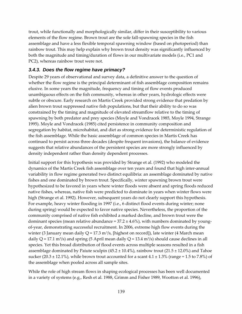
trout, while functionally and morphologically similar, differ in their susceptibility to various elements of the flow regime. Brown trout are the sole fall‐spawning species in the fish assemblage and have a less flexible temporal spawning window (based on photoperiod) than rainbow trout. This may help explain why brown trout density was significantly influenced by both the magnitude and timing/duration of flows in our multivariate models (i.e., PC1 and PC2), whereas rainbow trout were not.

3.4.3. Does the flow regime have primacy? Despite 29 years of observational and survey data, a definitive answer to the question of whether the flow regime is the principal determinant of fish assemblage composition remains elusive. In some years the magnitude, frequency and timing of flow events produced unambiguous effects on the fish community, whereas in other years, hydrologic effects were subtle or obscure. Early research on Martis Creek provided strong evidence that predation by alien brown trout suppressed native fish populations, but that their ability to do so was constrained by the timing and magnitude of elevated streamflow relative to the timing of spawning by both predator and prey species (Moyle and Vondracek 1985, Moyle 1994, Strange 1995). Moyle and Vondracek (1985) cited persistence in community composition and segregation by habitat, microhabitat, and diet as strong evidence for deterministic regulation of the fish assemblage. While the basic assemblage of common species in Martis Creek has continued to persist across three decades (despite frequent invasions), the balance of evidence suggests that relative abundances of the persistent species are more strongly influenced by density independent rather than density dependent processes.

Initial support for this hypothesis was provided by Strange et al. (1992) who modeled the dynamics of the Martis Creek fish assemblage over ten years and found that high inter‐annual variability in flow regime generated two distinct equilibria: an assemblage dominated by native fishes and one dominated by brown trout. Specifically, winter spawning brown trout were hypothesized to be favored in years where winter floods were absent and spring floods reduced native fishes, whereas, native fish were predicted to dominate in years when winter flows were high (Strange et al. 1992). However, subsequent years do not clearly support this hypothesis. For example, heavy winter flooding in 1997 (i.e., 6 distinct flood events during winter; none during spring) would be expected to favor native species. Nevertheless, the proportion of the community comprised of native fish exhibited a marked decline, and brown trout were the dominant species (mean relative abundance = 37.2 ± 4.6%), with numbers dominated by young‐of‐year, demonstrating successful recruitment. In 2006, extreme high flow events during the winter (3 January mean daily Q = 17.3 m3/s, [highest on record]), late winter (4 March mean daily Q = 17.1 m3/s) and spring (5 April mean daily Q = 13.4 m3/s) should cause declines in all species. Yet this broad distribution of flood events across multiple seasons resulted in a fish assemblage dominated by Paiute sculpin (45.2 ± 10.4%), rainbow trout (21.5 ± 12.0%) and Tahoe sucker (20.3 ± 12.1%), while brown trout accounted for a scant 4.1 ± 1.3% (range = 1.5 to 7.8%) of the assemblage when pooled across all sample sites.

While the role of high stream flows in shaping ecological processes has been well documented in a variety of systems (e.g., Resh et al. 1988, Grimm and Fisher 1989, Wootton et al. 1996),

139

droughts represent an important but understudied part of the flow regime which can dramatically alter community composition and ecosystem functioning (Bêche 2005, Bêche and Resh 2007, Power et al. 2008). Bêche et al. (2009) proposed that both the severity and duration of drought events are important in structuring invertebrate communities in Mediterranean‐type streams, and this appears to be equally true for the fish assemblage in Martis Creek. During dry water years, the amount of total available habitat is reduced, which presumably results in increased inter‐ and intraspecific competition. This is consistent with the finding of Propst et al. (2008) that native fish assemblages can persist through periods of drought, but their ability to do so is reduced when alien predators are present. In Martis Creek we would expect this to manifest as predation by brown trout, largely to the detriment of native species. However, while an isolated low water year may facilitate brown trout production, periods of prolonged drought appear to have a disproportionate negative effect on brown trout populations. This is most likely because brown trout live 5‐8 years in streams with only 1‐2 reproductive age classes, making them especially vulnerable to prolonged adverse conditions and the cumulative effects of reduced recruitment. While predation by alien brown trout has been reported to be a factor regulating fish abundance in many systems where they have been introduced, prolonged drought may explain why we found no evidence that brown trout density had a statistically significant effect on the density of other fish species over the complete period of study.

3.4.4. Climate change and the future of Martis Creek Climate change poses many uncertainties for the future of California’s native fish fauna. During the 21st century, average global surface temperature is projected to increase by 1.8‐4.0°C under different emission scenarios (IPCC 2007). Stream water temperature is often closely linked to air temperature and significant warming trends have already been documented in lotic ecosystems for which long‐term temperature data are available (Barnett et al. 2008, Kaushal et al. 2010). Mean weekly maximum water temperatures in Martis Creek generally range from 4°C to 21°C annually and temperatures during our late summer surveys averaged 18.0 ± 0.3°C (range = 12.0‐23.1°C, N = 80; P.B. Moyle unpublished data). While we found no significant effect of water temperature on the density of any species over the course of study, future warming is expected to principally stress sculpin and trout populations, while suckers and speckled dace will likely be unaffected (Moyle 2002). In addition to temperature effects, climate change is expected to produce appreciable changes to the local hydrology. Snowmelt discharge hydrographs like those that characterize Martis Creek and other alpine streams contain three major attributes that potentially affect the distribution and abundance of aquatic biota: peak flow, the spring pulse and base flow (Cayan et al. 2001). While climate change scenarios project little change to the total annual precipitation in California’s Sierra Nevada mountains, the region is expected to experience an advancement in the timing of precipitation events and an increase in the ratio of rain to snow (Knowles and Cayan 2002, Miller et al. 2003). This will result in more peak flows occurring during the winter, increased frequency of high flow events, diminished spring pulses, and protracted periods of low (base) flows.

We believe that a mixed native and non‐native assemblage will continue to persist into the future. However, rainbow trout may ultimately displace brown trout as the dominant predator in the system. Rainbow trout, like the endemic trout it replaced in the basin (Lahontan cutthroat

140

trout) is a spring spawning species and well adapted to the Mediterranean‐type flow regime. Results of our trend analyses indicated a positive increase in rainbow trout density and biomass at all sites over time, although trends were not always statistically significant (Table 3.5). The greatest disparity in density between the two trout species occurred in 1988 with average estimates of 103 ± 16 versus 6 ± 2 individuals/100m2 for brown trout and rainbow trout, respectively. Since that time, however, populations of the two species have exhibited markedly different trends with rainbow trout increasing in abundance and brown trout declining. Prior to the end of drought conditions in 1993, rainbow trout were only captured at all four sample sites during 5 (40%) of the annual collections. Since that time, however, rainbow trout have been documented at all sites during 90% of annual surveys and every year since 1996. During recent years the Martis Creek fish community appears to have exhibited a reversal in the abundance of rainbow trout and brown trout indicating the existence of a new alternate state in the system. This state may be closer to the original stream assemblage, given that the native cutthroat trout, like the related rainbow trout, spawns during the spring (Moyle 2002).

The effects of dams on the physical, hydrologic, and biologic characteristics of riverine ecosystems have been well documented (Ward and Stanford 1983, Ligon et al. 1995), and Martis Creek Dam and reservoir likely affect the downstream distribution and abundance of fishes. In addition to reducing extreme peak flows during the winter and spring, the Dam has altered the amount and temperature of water available during the summer low flow period. In 2005, the US Army Corps of Engineers designated Martis Creek Dam as one of the top six dams in the Nation in terms of risk due, in part, to an unacceptably high probability for seepage‐induced failure (USACE 2009). Seepage was first identified as a significant problem in 1995 and the water contributed to the creek is relatively cool because it originates from the bottom of the reservoir. Interestingly, the identification of dam seepage in 1995 roughly coincided with an increase in cool‐water species such as sculpin and rainbow trout, especially at the site immediately below the dam. Further, the augmented flow provided by seepage may help explain why no zero‐flow days occurred during our study and the IHA flow attribute ‘low pulse duration’ significantly declined over time.

3.4.5. Implications for stream fish assemblage studies and management of streams The contribution of long‐term data sets to our understanding of ecological pattern and process has long been recognized (e.g., Likens 1989, Magnuson 1990, Burt 1994). Often, judgments concerning community dynamics based on short time series of qualitative data or on irregular surveys spaced over time can be misleading. A principal tenet guiding studies of community persistence is that the length of the investigation should exceed at least one complete turnover of the constituent species (Connell and Sousa 1983) in order to avoid Frank’s (1968) tautology. However, our results clearly demonstrate that, for fish in lotic systems subjected to highly variable hydrologic regimes, annual samples collected over multiple decades may be necessary to successfully capture the full range of environmental conditions that influence assemblage dynamics. The data from Martis Creek led to different conclusions after 5, 10 and 30 years of study. Assemblage structure may be strongly influenced by the specific temporal sequence of stochastic hydrologic events (i.e., succession of wet and dry years) and multiple alternate states

141

may be possible, even in species‐depauperate systems. These results indicate the need for continuous annual monitoring of streams with altered flow regimes. Apparent successes or failures in stream management may appear in a different light under long‐term study.

142

4.0 Restoring Native Fish Assemblages to a Regulated California Stream Using the Natural Flow Regime Concept. Joseph D. Kiernan1 and Peter B. Moyle2, Center for Watershed Sciences, University of California, One Shields Avenue, Davis, CA 95616. 1 [email protected] 2 [email protected]

4.1. Introduction The flow regime of a stream is generally regarded as the ‘master variable’ that determines the composition of biotic assemblages (Poff and Ward 1989, Power et al. 1995, Matthews 1998). Nearly every other habitat factor that affects assemblage structure; from temperature, to water chemistry to physical habitat complexity, is determined by flow to a certain extent. The highly stochastic nature of natural flow regimes of most streams reduces predictability of assemblage structure (e.g., species composition), especially of fishes, but the predictability is at least partly a function of the scale (time, space) at which assemblage structure is examined (Matthews 1998). However, when streams are dammed and flow regimes are simplified by dam releases, stream fish assemblages also tend to become simplified and more predictable, usually dominated by selected species favored by fisheries (e.g., trout, Salmonidae) or by species that thrive in simplified habitats. Increasingly, this results in fish faunas in regulated streams becoming homogeneous and often depauperate, especially in North America and Europe (Moyle and Mount 2007, Poff et al. 2007). Recognition of this trend has led to the development of the concept of the Natural Flow Regime as a tool to restore native fish populations in regulated rivers, with diverse methods being developed to apply the concept to river management (Poff et al. 1997, Poff and Zimmerman 2010).

In California, most streams are dammed or diverted, causing drastic changes in flow regimes. One result has been the collapse of native fish populations; nearly 60% of California’s 129 native inland fish species are extinct or have population trends suggesting extinction is likely in the coming decades (Moyle et al. forthcoming37). In many highly altered regulated streams, native fishes have been replaced by alien species better adapted for changed conditions such as more constant flows, poorer water quality, and less habitat complexity (Moyle 2002, Moyle and Marchetti 2006). Therefore, one relatively good measure of the success of a ‘natural’ flow regime established in a regulated river is the return of native fishes as dominant species.

Here we examine the response of the fishes of lower Putah Creek (Yolo and Solano counties, California) to the establishment of a flow regime prescribed as the result of a legal action to restore flows in order to re‐establish native fishes to a once‐dry stream (Moyle et al. 1998). Marchetti and Moyle (2001) demonstrated the potential for recovery of native fishes in much of Putah Creek following a series of wet years that fortuitously followed the original 1996 court decision to restore flows to the creek. A negotiated settlement (hereafter Accord) was reached in 2000 that determined the actual flow regime, which was based on the natural flow regime concept. Annual monitoring of the fish populations was also part of the agreement, in order to determine if the native fishes would, in fact, respond to the new flow regime. The flow regime

37 Working paper available online: http://watershed.ucdavis.edu/library.html

143

http://watershed.ucdavis.edu/library.html

required only a small percentage of available water in most years, so the flows were ‘natural’ only in timing, and not in volume. In this paper, we ask: was the new flow regime successful at 1) re‐establishing native fishes to lower Putah Creek and 2) reducing abundances of alien fishes under typical operating conditions (e.g., no spills from upstream dams)? Because the flows diminish as a function of distance from dam releasing the water, we could also ask 3) under what conditions the alien fishes resume dominance of the fish assemblages?

4.1.1. Putah Creek Flow Accord The flow Accord, signed in May 2000, immediately created a new permanent schedule of minimum flow releases from Putah Diversion Dam into lower Putah Creek. Briefly, of the six elements of the Accord, three were specifically designed to benefit fish and other aquatic organisms:

1) Rearing and spawning flows for resident native fish ‐ This established a baseline flow necessary to maintain a year‐round living stream from Putah Diversion Dam (PDD) to the Yolo Bypass (ca. 37 km). Rearing flows were intended to provide, at a minimum, several km of cool‐water habitat for native fishes below PDD, even under drought conditions. Additionally, it was intended to provide sufficient water to support introduced game fishes (e.g., bluegill, catfishes, and largemouth bass) in the lower reaches. Spawning flows consist of a short 3 day pulse between February–March, to initiate spawning behavior, followed by a month‐long release of elevated (i.e., higher than baseline) flows. The rationale behind this schedule was to provide spawning opportunities for native fishes in the winter and spring of dry water years.

2) Supplemental flows to attract and support anadromous fishes ‐ Supplemental (pulse) flows

were included to promote the migration of fall‐run Chinook salmon, and other anadromous species. The Accord included a requirement for a minimum flow beginning in mid‐November and a 5‐day pulse flow in November or December (actual date based on escapement monitoring) to attract and enable adult Chinook salmon to migrate up Putah Creek from the Yolo Bypass. Additionally, the Accord also specified springtime minimum flows designed to benefit juvenile salmon rearing and facilitate outmigration.

3) Drought year flows ‐ A drought schedule was created to guarantee a continuous flow in

the segment from PDD to Interstate‐80 (ca. 24 km) at all times, even when water levels were low in the upstream reservoir. This was intended to protect native fish assemblages that were known to reside in reaches closer to the Diversion Dam (e.g., Moyle et al. 1998, Marchetti and Moyle 2000, Marchetti and Moyle 2001).

4.2. Methods 4.2.1. Study area This study was conducted in lower Putah Creek, a tributary of the Sacramento River in Yolo and Solano Counties, California, USA (Fig. 4.1). Putah Creek originates in the Coast Range of California and flows freely east for ca. 130 km before being impounded by Monticello Dam, forming Berryessa Reservoir (surface area = 8,400 ha; storage capacity = 1.98 km3). Water

144

releases from Monticello Dam flow ca. 13 km to a second dam, Putah Diversion Dam. The stream section below Putah Diversion Dam is deemed lower Putah Creek and flows ca. 37 km before eventually joining the Sacramento River (Marchetti and Moyle 2001).

Figure 4.1. Map of lower Putah Creek, Yolo and Solano counties, California, and fish sample sites. Key to sample site abbreviations: D = Putah Diversion Dam, I = Interstate 505, S = Stevenson Bridge Road, P =Pedrick Road, O = Old Davis Road, and M = Mace Boulevard. Figure modified from Marchetti and Moyle (2001). Streamflow in lower Putah Creek is regulated during most of the year except when large rainfall events cause Berryessa Reservoir to spill uncontrollably. Spill events can occur at any time of the year between December and June (Fig. 4.2) and, combined with flows from tributaries upstream and downstream of Putah Diversion Dam, cause substantial pulses of water to move through lower Putah Creek. The maximum recorded mean daily discharge from Monticello Dam during the period of study was 399.0 m3/s on 26 January 1997 (USGS gage No.11454000; http://waterdata.usgs.gov) which resulted in a mean daily discharge of 325.0 m3/s from Putah Diversion Dam into the lower creek during the following day.

4.2.2. Fish sampling: In 1991, six stream reaches were selected as representative of typical habitats in the lower creek and established as permanent sample sites. The six sites: Putah Diversion Dam (D), Interstate 505 (I), Stevenson Bridge Road (S), Pedrick Road (P), Old Davis Road (O), and Mace Boulevard (M), were located 0.1, 6.2, 14.5, 20.5, 25.0 and 30.3 km downstream of Putah Diversion Dam, respectively. All sites were sampled annually from 1991‐2008 (except 1992) in September or October during low (base) flow conditions. Fish were captured using either a backpack or boat electrofisher depending on habitat conditions. Captured fish were identified to species and measured for standard length (± 1.0 mm). Biomass was determined by water displacement or by weighing with a Pesola spring scale (± 1.0 g; Pesola AG, Baar, Switzerland). Fish species that were either 1) present in < 5 of the annual samples or 2) did not constitute at least 5% of the total assemblage at any site were deemed rare and excluded from all analyses. Unidentified sunfish

145

and hybrids among all species (i.e., green sunfish × bluegill, green sunfish × redear sunfish, and redear sunfish × bluegill), were grouped as Lepomis spp. in all analyses.

Dis

char

ge (m

3 /s)

0.1

1

10

100

1000

Oct Nov Dec Jan Feb Mar Apr May Jun Jul Aug Sep

1991

1992

1993

1994

1995

19

96

1997

19

98

1999

2000

2001

20

02

2003

2004

2005

2006

20

07

2008

Mea

n da

ily d

isch

arge

(m3 /s

)

0.1

1

10

100

A.

B.

WYT = C C C CAN AN ANANW W WW W D D WBN D

Figure 4.2. Flow regime for Lower Putah Creek, California, USA. (A) Mean daily discharge from the Putah Diversion Dam during the period of study, 1991-2008. Water year types (WYT) are defined as wet (W), above normal (AN), below normal (BN), dry (D) and critical (C). (B) Summary of discharge for each day of the water year based on the complete period of record (N = 31 years): solid line = mean discharge, gray shaded region = range of discharge values.

4.2.3. Data analysis: Hydrology To determine trends in streamflow in lower Putah Creek, records of mean daily flow releases from the Putah Diversion Dam (water years 1977‐2008) were obtained from Solano County Irrigation District (Elmira, Calif.). We used the Indicators of Hydrologic Alteration (IHA) model of Richter et al. (1996) to contrast the periods 1977‐1999 (pre‐Accord) and 2000‐2008 (post‐

146

Accord), and assess how select attributes of the flow regime were affected by implementation of the flow Accord. The IHA model uses daily discharges values to calculate 33 indices representing five broad categories: (1) flow magnitude; (2) magnitude and duration of annual extreme conditions; (3) timing of annual extreme conditions; (4) frequency and duration of high and low pulses; and (5) rate and frequency of changes in conditions (The Nature Conservancy 2007).

Fish Assemblages Two‐way cluster analysis was used to assess similarity in fish assemblages among sample sites and years. Clusters were based on Bray‐Curtis similarity and employed flexible linkage methods (β = ‐0.25). We generated separate cluster dendrograms and matrices for both the pre‐ (1991‐1999) and post‐Accord (2000‐2008) periods. Non‐metric multidimensional scaling (nMDS) ordinations were then used to examine patterns in assemblage composition among the six sample sites during each period. For this analysis, Bray‐Curtis similarities were calculated on log10(x + 1) transformed fish abundance data and nMDS was used to ordinate sites based on similarities in fish assemblages. We followed the recommendation of McCune and Grace (2002) and used multiple runs of our real data (N=100 runs) to avoid local stress minima, and used 1000 Monte Carlo simulation runs to assess the significance of our final two ordination axes. In ordination plots, sites are presented as ellipses which represent the 95% confidence interval surrounding the mean position of each sample site in ordination space. Distances between sites are proportional to the overall similarity of their fish assemblages. Cluster and nMDS analyses were performed with PC‐ORD version 5.1 (MjM Software Design, Gleneden Beach, Oregon, USA)

MRPP We used a nonparametric multi‐response permutation procedure (MRPP) to test the null hypothesis of no differences in species composition among the 6 sample sites. MRPP is recommended for ecological data because it does not require assumptions of normality and constant variance (McCune and Grace 2002, Biondini et al. 1988). Euclidean distances within and between sample sites were calculated on untransformed abundance data. We used the weighting factor recommended by Mielke (1984) and rare species were excluded from the analyses to reduce noise and improve the correlation structure. MRPP produces two statistics: an A‐statistic describing the effect size of the grouping and a P‐value which estimates the probability that observed differences are due to chance (McCune and Grace 2002). An overall significant test (P < 0.05) was followed by pair‐wise comparisons of all possible sites (N=15). Significant differences between sites were assessed using a Bonferroni adjusted type I error rate (α) of 0.003 (0.05/15). Separate MRPP analyses were conducted for the pre‐ and post‐Accord periods.

Indicator value analysis To determine the most representative fish species at each sample site, we used indicator value analysis (Dufrêne and Legendre 1997). Indicator species are defined as those that express the highest degree of specificity and fidelity to a site, independent of abundance (Dufrêne and Legendre 1997). The maximum possible indicator value (100) occurs when all individuals of a

147

given species are found at a single site and when the species is present during every survey year. The statistical significance (P < 0.05) of the species’ indicator values is evaluated based on the proportion of 9999 randomized trials that equaled or exceeded the maximum indicator value observed (Monte Carlo test).

4.3. Results 4.3.1. Hydrology: The flow regime in lower Putah Creek exhibited high inter‐annual variability during the period of study (Fig. 4.2), chiefly due to precipitation events that caused Monticello Dam to spill. Of the 18 water years encompassed by our study, 6 were classified by the California Department of Water Resources38 as wet, 4 as above normal, 1 as below normal, 3 as dry and 4 as critically dry (Fig. 4.2a). The implementation of the flow Accord had a marked effect on the magnitude, duration and timing of stream flows in lower Putah Creek (Table 4.1). Mean monthly streamflow during the post‐Accord period increased for eight months of the water year with the greatest percentage gain occurring in the spring (April = +47% and May = +63%; Table 4.1a). Additionally, the new flow regime changed the magnitude and duration of annual extremes with mean 1, 3, 7, 30, and 90‐day minimum flows all increasing. Mean maximum flows calculated for these same intervals decreased (Table 4.1b), but this reflects natural inter‐annual variability in precipitation rather than operation of the diversion dam. Finally, both the mean count and duration of low‐flow pulses decreased in the post‐Accord period (Table 4.1d).

4.3.2. Fish Species: In total, 35 distinct39 fish species (13 native; 37%) were captured in lower Putah Creek between 1991 and 2008. Of the 13 fish families collected, the Centrarchidae (N =10 species, 1 native), Cyprinidae (N = 8 species, 4 native), and Ictaluridae (N = 4 species, all alien) were most speciose (Table 4.2.). Our late summer sampling captured 90% of the taxa known to occur in the creek (P. B. Moyle, unpublished data). The seven fish species collected during our study but considered rare based on presence (≤ 5 of the annual samples) or abundance (< 5% of the total assemblage at any site) and excluded from subsequent analysis were: Sacramento perch, spotted bass, yellowfin goby, brown bullhead, striped bass, Chinook salmon, and brown trout (Table 4.2).

38 California Department of Water Resources water year classification index for the Sacramento Valley. Available online at: http://cdec.water.ca.gov/cgi‐progs/iodir/WSIHIST 39 Excludes hybrids

148

http://cdec.water.ca.gov/cgi-progs/iodir/WSIHIST

Table 4.1. Results of the Indicators of Hydrologic Alteration analysis for lower Putah Creek contrasting select attributes of the flow regime before and after alteration of the flow regime.

%Mean SD CV Mean SD CV

A. Monthly streamflow (m3/s)October 0.59 0.15 0.25 0.64 0.12 0.18 7.39November 0.78 0.17 0.21 0.89 0.15 0.17 14.31December 2.93 8.99 3.07 1.83 1.41 0.77 ‐37.63January 10.91 25.28 2.32 9.94 27.12 2.73 ‐8.88February 23.84 51.23 2.15 14.09 24.50 1.74 ‐40.91March 22.59 48.11 2.13 24.47 31.83 1.30 8.30April 12.21 30.49 2.50 18.01 33.54 1.86 47.43May 2.43 4.44 1.83 3.96 4.59 1.16 63.11June 1.45 1.48 1.03 1.27 0.15 0.11 ‐12.54July 1.15 0.16 0.14 1.22 0.00 0.00 6.07August 0.92 0.11 0.12 0.97 0.01 0.01 5.45September 0.63 0.15 0.24 0.66 0.14 0.20 5.00Mean change (%) 21.40

B. Magnitude and duration of annual extremes1‐day minimum 0.44 0.09 0.21 0.47 0.04 0.08 4.973‐day minimum 0.45 0.09 0.21 0.47 0.04 0.08 4.657‐day minimum 0.46 0.08 0.18 0.48 0.04 0.09 6.2530‐day minimum 0.52 0.08 0.15 0.56 0.05 0.09 7.2590‐day minimum 0.72 0.14 0.20 0.79 0.14 0.17 10.321‐day maximum 103.40 132.43 1.28 88.12 119.19 1.35 ‐14.743‐day maximum 89.56 121.81 1.36 73.25 98.24 1.34 ‐18.217‐day maximum 73.99 105.50 1.43 59.68 75.24 1.26 ‐19.3330‐day maximum 46.52 70.52 1.52 35.33 41.58 1.18 ‐24.0590‐day maximum 23.36 36.91 1.58 19.59 24.93 1.27 ‐16.13No. zero flow days 0.00 0.00Base flow index 0.29 0.21 0.73 0.21 0.18 0.86 ‐26.57Mean change (%) 13.90

C. Timing of annual extremesJulian date of minimum 134.50 119.70 0.33 59.67 285.23 0.22 40.91Julian ate of maximum 54.76 50.80 0.14 44.67 319.73 0.13 5.52Mean change (%) 23.20

D. Frequency and duration of high and low flowsLow pulse count 3.95 2.48 0.63 3.33 1.87 0.56 ‐15.66Low pulse duration 27.54 15.45 0.56 20.09 13.30 0.66 ‐27.05High pulse count 1.33 1.49 1.12 0.67 0.71 1.06 ‐50.00High pulse duration 11.25 9.71 0.86 17.90 16.68 0.93 59.11Low Pulse Threshold 0.71High Pulse Threshold 34.79Mean change (%) 38.00

E. Rate and frequency of changes in flowRise rate 7.33 9.51 1.30 5.66 1.18 ‐22.76Fall rate ‐3.60 3.22 ‐0.90 ‐2.45 ‐0.95 ‐31.94Number of reversals 26.90 13.88 0.52 27.56 0.47 2.42Mean change (%) 19.00

1979‐1999change

2000‐2008

149

Table 4.2. Fish species collected at six permanent sample sites in lower Putah Creek, California, USA.

Family Taxon FeedingScientific name Common name code Origin guild D I S P O M

AtherinopsidaeMenidia beryllina Inland silverside ISS I IS ○ ○ ◑ ◑ ◑

CatostomidaeCatastomus occidentalis Sacramento sucker SKR N O ◑ ◑ ◑ ◑ ◑ ◑

CentrarchidaeArchoplites interruptus Sacramento perch † N IL ● ◑Lepomis cyanellus Green sunfish GSF I IL ◑ ◑ ◑ ◑ ◑ ◑Lepomis gulosus Warmouth WRM I IL ◑ ◑Lepomis macrochirus Bluegill BGS I IS ◑ ◑ ◑ ◑ ◑ ◑Lepomis microlophus Redear sunfish RES I IS ● ● ◑ ◑ ○Lepomis spp. Various‡ LEP I IS ◑ ● ◑ ◑ ◑ ◑Micropterus dolomieu Smallmouth bass SMB I P ◑ ◑ ◑ ◑ ◑ ○Micropterus punctulatus Spotted bass † I P ○ ○Micropterus salmoides Largemouth bass LMB I P ◑ ◑ ◑ ◑ ◑ ◑Pomoxis nigromaculatus Black crappie BCR I IS ● ● ● ◑

CottidaeCottus asper Prickly sculpin PSC N IS ◑ ◑ ◑ ◑ ○ ◑Cottus gulosus Riffle sculpin RSC N IS ◑ ◑ ○ ○

CyprinidaeCarassius auratus Goldfish GLF I O ● ● ◑ ● ◑ ◑Cyprinella lutrensis Red shiner RSH I IS ◑ ◑ ◑ ◑Cyprinus carpio Common carp CRP I O ◑ ● ◑ ◑ ◑ ◑Lavinia exilicauda Hitch HTC N IS ◑ ◑ ◑ ◑ ● ◑Lavinia symmetricus California roach RCH N O ◑ ●Orthodon microlepidotus Sacramento blackfish SBF N AD ● ● ● ◑Pimephales promelas Fathead minnow FHM I O ● ◑Ptychocheilus grandis Sacramento pikeminnow PKM N P ◑ ◑ ◑ ◑ ◑ ◑

EmbiotocidaeHysterocarpus traski Tule perch TUP N IS ◑ ◑ ◑ ◑ ◑ ●

GasterosteidaeGasterosteus aculeatus Threespine stickleback SBK N IS ◑ ◑ ●

GobiidaeAcanthogobius flavimanus Yellowfin goby

●◑

† I IL ○Ictaluridae

Ameiurus catus White catfish WCF I IL ● ◑ ○ ○ ◑Ameiurus melas Black bullhead BBH I O ◑ ● ◑ ● ◑Ameiurus nebulosus Brown bullhead † I IS ● ● ●Ictalurus punctatus Channel catfish CCF I P ● ◑ ◑

MoronidaeMorone saxatilis Striped bass † I P ◑

PercidaePercina macrolepida Bigscale logperch BLP I IS ◑ ◑ ◑ ◑ ◑ ◑

PetromyzontidaeLampetra tridentata Pacific lamprey PLR N AD ◑ ◑ ◑ ◑ ○ ○

PoeciliidaeGambusia affinis Western mosquitofish MSQ I IS ◑ ◑ ◑ ◑ ◑ ◑

SalmonidaeOncorhynchus mykiss Rainbow trout RBT N IS ◑ ○ ●Oncorhynchus tshawytscha Chinook salmon † N IS ●Salmo trutta Brown trout † I IS ○

Sample site

Notes: Open circles (○) indicate a given taxon was present ≥ 1 of the pre‐Accord (1991‐1999) surveys exclusively, filled circles (●) indicate presence ≥ 1 of the post‐Accord (2000‐2008) surveys exclusively, and semi‐filled circles (◑) signify presence during both pre‐ and post‐Accord periods. Origin abbreviations: N = native and I = introduced. Feed guild abbreviations: AD = algivores and detritivores; IS = small prey (< 10 mm length) invertivores; IL = large prey (≥10 mm length) invertivores; O = omnivores; and P = piscivores. † Excluded from cluster analyses and ordinations due to rarity (see methods). ‡ The group Lepomis spp. includes Pumkinseed (Lepomis gibbosus) and centrarchid hybrids.

150

Information Remaining (%)0 25 50 75 100

100

7550

250

D-91D-96D-97D-93D-94D-95D-98D-99I-98I-99P-99S-98S-99P-98S-97I-96I-91I-97I-95I-93I-94O-97O-99S-91S-96S-93P-93P-97M-99S-94M-93M-95O-94P-91O-95O-91O-96P-94M-96O-93M-97O-98S-95M-98P-95P-96M-91M-94

SB

K*

PS

C*

RS

C*

RB

T*S

KR

*R

CH

*H

TC*

PK

M*

PLR

*C

CF

RS

HW

CF

WR

MTU

P*

SM

BR

ES

BLP

GS

FLM

BS

BF*

BB

HB

CR

BG

SG

LFIS

SC

RP

LEP

FHM

MS

Q

Matrix Coding

MaxMin

Figure 4.3. Two-way cluster analysis of species abundances and sample events (sites and years) prior to implementation of the flow Accord, 1991-1999. Species abbreviations used along the top of matrix are defined in Table 4.2. Native species are denoted with asterisks. Sample site codes (left side of matrix) are: D = Putah Diversion Dam, I = I-505, S = Stevenson Bridge, P = Pedrick Rd., O = Old Davis Rd., M = Mace Blvd., followed by a two-digit abbreviation for the sample year (e.g., 91 = 1991).

151

Information Remaining (%)0 25 50 75 100

100

7550

250

D-00D-05D-01D-04D-06D-03D-02D-07D-08I-08I-00I-04I-03I-05I-06I-07I-01I-02S-07S-02S-03S-04S-05S-00S-08P-05P-03S-01P-06S-06P-00P-08P-01P-07P-04O-00M-03O-05O-06O-03O-04O-01O-07O-02M-02P-02M-01O-08M-08M-00M-04M-05M-06M-07

SB

K*

RS

C*

RB

T*R

CH

*P

LR*

HTC

*P

SC

*S

KR

*P

KM

*TU

P*

SM

BS

BF*

CR

PB

CR

FHM

MS

QR

SH

CC

FB

GS

GS

FLE

PB

LPR

ES

ISS

LMB

WC

FB

BH

GLF

WR

M

Matrix Coding

MaxMin

Figure 4.4. Two-way cluster analysis of species abundances and sample events (sites and years) after implementation of the flow Accord, 2000-2008. Species abbreviations used along the top of the matrix are defined in Table 4.2. Native species are denoted with an asterisk. Sample site codes (left) are followed by a two-digit abbreviation for the sample year (e.g., 00 = 2000). Site codes are defined in Fig. 4.3.

152

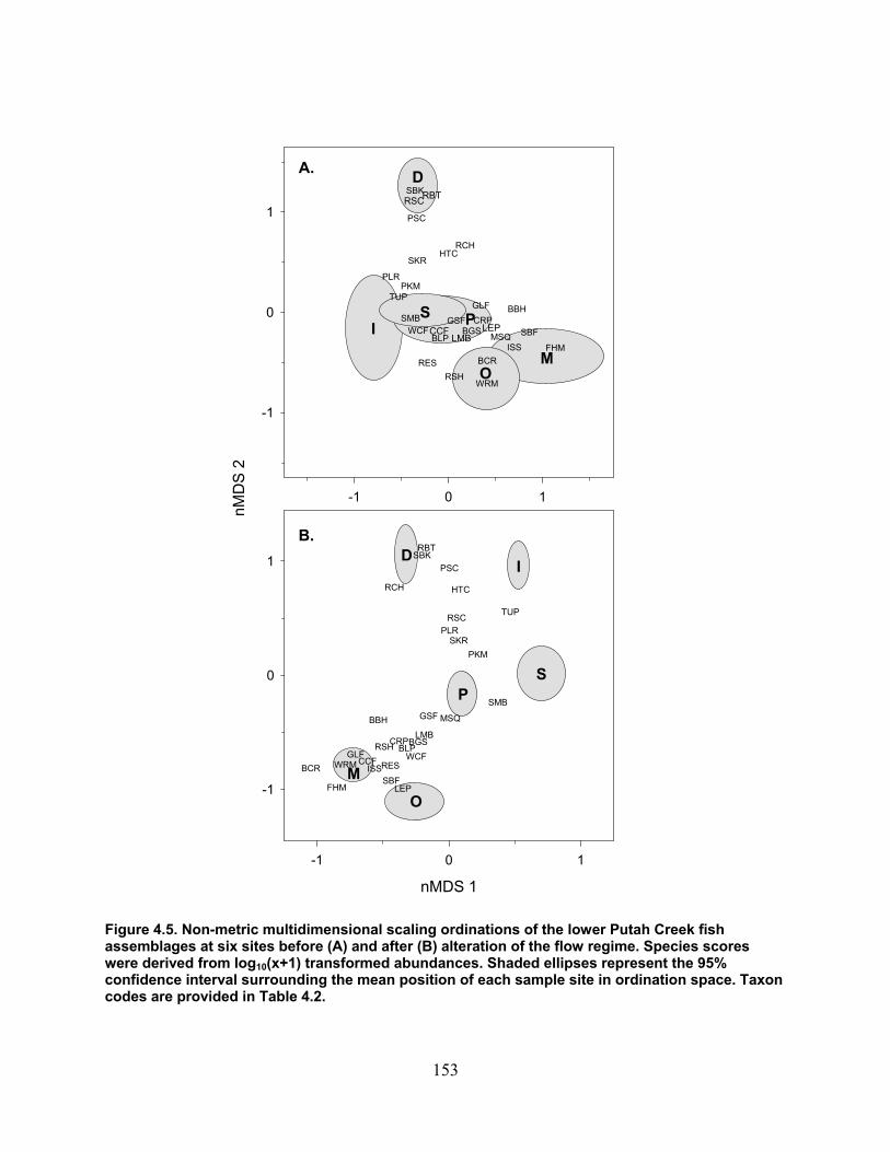
-1 0 1

-1

0

1

LEPCRP SP

BBH

BCR

BGSBLP

CRP

FHM

GLF

GSF

HTC

ISSMSQ

PKMPLR

PSC

RCH

RESRSH

SBF

SBK

SKR

SMB

TUP

WCF

WRM

DRBTRSC

LEPCCFLMB

IS P

OM

nMDS 1

-1 0 1

nMD

S 2

-1

0

1

BBH

BCR

BLPCRP

GLF

GSF

HTC

LMB

MSQ

PKM

PLRRSC

RCH

RES

PSC

RSH

SBF

SBK

SKR

SMB

TUP

WCFWRM

LEPFHM

RBT

CCF

BGS

ISS

DI

SP

O

M

A.

B.

Figure 4.5. Non-metric multidimensional scaling ordinations of the lower Putah Creek fish assemblages at six sites before (A) and after (B) alteration of the flow regime. Species scores were derived from log10(x+1) transformed abundances. Shaded ellipses represent the 95% confidence interval surrounding the mean position of each sample site in ordination space. Taxon codes are provided in Table 4.2.

153

4.3.3. Fish Assemblages: Two‐way cluster analysis for the pre‐Accord period revealed a strong pattern of association between native fish species and the Putah Diversion Dam site, and a centrarchid dominated assemblage at the I‐505 site (Fig. 4.3). Additionally, The I‐505, Stevenson Bridge and Pedrick Rd. sites formed a distinct cluster during years 1998 and 1999. Beyond these relationships, however, there were few clear spatial or temporal patterns to the grouping of sample sites or fish species. This suggests homogenous physical and biological conditions throughout much of the creek supporting assemblages dominated by alien species (Fig. 4.3). Results of cluster analysis conducted on the post‐Accord abundance data illustrated a strong shift in the longitudinal distribution of fishes within the creek. Most notably, native taxa were increasingly abundant, especially at the 3 sample sites immediately below Putah Diversion Dam (i.e., I‐505, Stevenson Bridge and Pedrick Rd.; Fig. 4.4)

The NMDS analyses for each time period indicated that two‐dimensional ordinations were optimal, with both axes serving as significant predictors (P ≤ 0.001) of species composition. Collectively, the two axes explained 89% and 94% of the variation in species composition among sites for the pre‐Accord and post‐Accord periods, respectively. For the pre‐Accord period, sample sites clustered along a longitudinal gradient on Axis 1 of the ordination diagram with upstream sites loading negatively and downstream sites loading more positively (r2 for Axis 1 = 0.4040; Fig. 4.5a). Fish species most positively correlated (Pearson) with the first axis were fathead minnow (r = 0.70), western mosquitofish (r = 0.66), Sacramento blackfish (r = 0.62) bluegill (r = 0.60), and inland silverside (r = 0.53). The second axis separated the Putah Diversion Dam site from all downstream study locations (r2 for Axis 2 = 0.49). Fish species most positively correlated with Axis 2 were all native: Sacramento sucker (r = 0.84), threespine stickleback (r = 0.82) prickly sculpin (r = 0.80) riffle sculpin (r = 0.80), hitch (r = 0.69), and rainbow trout (r = 0.69).

Sample sites during the post‐Accord period exhibited considerably more separation in ordination space relative to the pre‐Accord period (Fig. 4.5). In general, species associations with each nMDS axis were weaker during the post‐Accord period suggesting increased heterogeneity with respect to physical and chemical conditions in the creek. Species most positively correlated with the first axis (r2 = 0.20) during the post‐Accord period were Tule perch (r = 0.71), Sacramento pikeminnow (r = 0.63), and smallmouth bass (r = 0.45). Taxa most positively correlated with the Axis 2 (r2 = 0.74) were largely coldwater natives: prickly sculpin (r = 0.76), riffle sculpin (r = 0.72) rainbow trout (r = 0.67), and threespine stickleback (r = 0.63) (Fig. 4.5b).

Pair‐wise MRPP comparisons of all sample sites during the pre‐Accord period revealed similarity in the fish assemblages at some sample sites. Specifically, the fish assemblage at I‐505 site was not statistically different from that at the Stevenson Road site (A= 0.06, P = 0.020), Mace Blvd. site was similar to the Old Davis Rd. site (A= 0.03, P = 0.093), and species composition at

40 Coefficient of determination for the correlations between ordination distances and distances in the original n‐dimensional space.

154

the Pedrick Rd. site did not differ from that at the Stevenson Rd. (A= 0.03, P = 0.133), Old Davis Rd. (A= 0.05, P = 0.039), or Mace Blvd. sample sites (A= 0.03, P = 0.052; Table 4.3). Only four of the sample sites during the pre‐Accord period contained taxa that received high indicator values (Putah Diversion Dam, I‐505, Stevenson Rd., and Mace Blvd.; Table 4.4). Of these, Putah Diversion Dam was the only site characterized by indicator species that were exclusively native. In contrast, pair‐wise MRPP comparisons conducted for the post‐Accord period indicated that fish assemblages at all sample sites were statistically different form each other after Bonferroni adjustment (all sites P < 0.003; Table 4.3). Moreover, all six sites contained one or more species with significant indicator scores (Table 4.4), and three of theses sites (Putah Diversion Dam, I‐505, Pedrick Rd.) were represented by native taxa exclusively (Table 4.4). Table 4.3. Matrix of A-values derived from multi-response permutation procedure (MRPP) contrasting the fish assemblages at six sample before (upper-half of matrix) and after (lower-half of matrix) alteration of the flow regime.

Sample site D I S P O M D — 0.19 0.17 0.21 0.31 0.21 I 0.22 — 0.06 0.09 0.19 0.13 S 0.29 0.18 — 0.03 0.15 0.09 P 0.27 0.23 0.12 — 0.05 0.03 O 0.35 0.37 0.33 0.31 — 0.03 M 0.34 0.36 0.33 0.29 0.08 —

Notes: MMPRs A‐statistic describes degree of within‐group homogeneity compared to that expected by chance (i.e., effect size). The value of A ranges from 0.0 when heterogeneity within sample sites equals that expected by chance, to 1.0 when assemblages at each sample site are identical. If heterogeneity within groups is more than expected by chance A > 0. Bold values indicate significant differences (Bonferroni adjusted α = 0.003) between the fish assemblages when contrasting sample site pairs. Site abbreviations are: D = Putah Diversion Dam, I = I‐505, S = Stevenson Bridge, P = Pedrick Rd., O = Old Davis Rd., M = Mace Blvd.

4.3.4. Flow Regime The flow regime of lower Putah Creek had a substantial influence on the temporal and spatial distribution of native fish populations during our study. While the Putah Diversion Dam sample station was largely dominated by native species across both the pre‐ and post‐Accord periods (Fig. 4.6), native species resumed dominance of the mid‐reaches of lower Putah Creek as a result of consecutive wet years that generated large natural stream flows (i.e., 1997‐1999) and subsequent implementation of the flow Accord (Fig. 4.6). The magnitude and timing of flows were especially important to the maintenance of native fish assemblages. We found a positive relationship between mean spring discharge (1 March through 30 May) and the proportion of the fish assemblage composed of native species at the 4 upstream‐most sites, though this relationship was only statistically significant at the Stevenson Rd. (r2 = 0.30, F[1,17] = 6.76, P = 0.02) and Pedrick Rd. sites (r2 = 0.36, F[1,17] = 9.14, P < 0.01; Fig. 4.7). Additionally, the proportional abundance of native fishes at the two middle sites was significantly and positively

155

related to annual 7‐day maximum discharge (Stevenson Rd.: r2 = 0.24, F[1,17] = 5.08, P = 0.04 and Pedrick Rd.: r2 = 0.23, F[1,17] = 4.81, P = 0.04; Fig. 4.8). Table 4.4. Indicator value (IV) scores and associated P-values obtained by Monte Carlo permutations for fish taxa at the 6 permanent sample sites. Indicator species were determined separately for the pre- (1991-1999) and post-Accord (2000-2008) periods.

Sample site Taxon IV P IV PPutah Diversion Dam Threespine stickleback† 99.0 <0.001 98.2 <0.001

Rainbow trout† 81.8 <0.001 96.4 <0.001Sacramento sucker† 63.9 <0.001 36.0 0.022Hitch† 61.5 0.002 34.8 0.026Riffle sculpin† 48.6 0.003 81.8 <0.001Prickly sculpin† 42.6 0.007 43.5 <0.001Pacific lamprey† 33.9 0.022 29.2 0.039

I-505 Tule perch† 51.6 <0.001 87.9 <0.001Smallmouth bass 46.6 0.002 . . . . . .Redear sunfish 36.5 0.014 . . . . . .

Stevenson Bridge Smallmouth bass . . . . . . 71.1 <0.001

Pedrick Rd. Sacramento pikeminnow† . . . . . . 61.1 <0.001

Old Davis Rd. Bluegill . . . . . . 53.5 <0.001Lepomis spp.‡ 26.5 0.004Green sunfish . . . . . . 29.4 0.049

Mace Blvd. Western mosquitofish 86.5 0.003 . . . . . .Fathead minnow 84.5 <0.001 54.5 0.001Inland silverside 56.6 0.003 63.3 <0.001Sacramento blackfish† 41.3 0.006 . . . . . .Red shiner . . . . . . 84.2 <0.001Goldfish . . . . . . 64.6 <0.001Redear sunfish . . . . . . 44.5 0.006Warmouth . . . . . . 41.8 0.007Channel catfish . . . . . . 39.5 0.007Largemouth bass . . . . . . 36.2 0.006Common carp . . . . . . 31.7 0.015White catfish . . . . . . 30.3 0.016

Pre-accord Post-accord

Note: Only the characteristic species for each location (i.e., P<0.05) are presented. P‐values represent the proportion of randomized trials (N = 9999) with an indicator value equal to or exceeding the observed indicator value. † Indicates native species.

156

Putah Diversion Dam

Tota

l fis

hab

unda

nce

0

500

1000

1500

2000

Interstate505 Bridge

Stevenson Road Bridge

Pedrick Road

Old Davis Road

Mace Boulevard

Prop

ortio

n na

tive

spec

ies

0.00.20.40.60.81.0

1991

1993

1995

1997

1999

2001

2003

2005

2007

Taxo

nric

hnes

s

0

5

10

15

20

1991

1993

1995

1997

1999

2001

2003

2005

2007

1991

1993

1995

1997

1999

2001

2003

2005

2007

1991

1993

1995

1997

1999

2001

2003

2005

2007

1991

1993

1995

1997

1999

2001

2003

2005

2007

1991

1993

1995

1997

1999

2001

2003

2005

2007

Water Year Figure 4.6. Time series of annual total fish abundance, proportion of native species and taxon richness at each sample site, 1991-2008. Gray shaded region indicates samples collected prior to implementation of the flow Accord in 2000.

Putah Diversion Dam

0.0

0.2

0.4

0.6

0.8

1.0I-505

0.0

0.2

0.4

0.6

0.8

1.0Stevenson Rd.

Prop

ortio

n na

tive

spec

ies

0.0

0.2

0.4

0.6

0.8

1.0

Pedrick Rd.

0.0 0.5 1.0 1.5 2.00.0

0.2

0.4

0.6

0.8

1.0

0.0 0.5 1.0 1.5 2.00.0

0.2

0.40.8

1.0Old Davis Rd.

Mean spring discharge (log10 m3/s + 1)0.0 0.5 1.0 1.5 2.0

0.0

0.2

0.40.8

1.0Mace Blvd.

r2= 0.00P = 0.98

r2= 0.17P = 0.09 r2= 0.30

P = 0.02

r2= 0.36P < 0.01

r2= 0.00P = 0.77

r2= 0.18P = 0.08

Figure 4.7. Relationship between mean spring (1 March through 30 May) discharge and the proportion of the total fish assemblage comprised of native species at each sample site. Proportion data were arcsine square-root transformed prior to regression analysis.

157

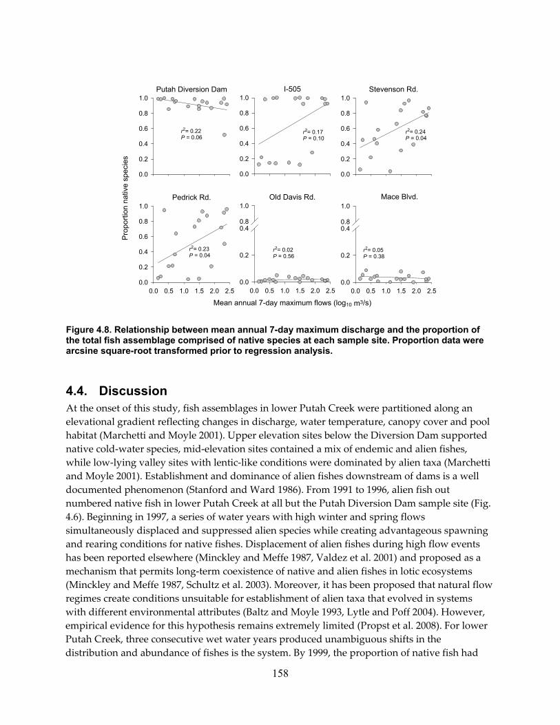
Putah Diversion Dam

0.0

0.2

0.4

0.6

0.8

1.0I-505

0.0

0.2

0.4

0.6

0.8

1.0Stevenson Rd.

Pro

porti

on n

ativ

e sp

ecie

s

0.0

0.2

0.4

0.6

0.8

1.0

Pedrick Rd.

0.0 0.5 1.0 1.5 2.0 2.50.0

0.2

0.4

0.6

0.8

1.0

0.0 0.5 1.0 1.5 2.0 2.50.0

0.2

0.40.8

1.0Old Davis Rd.

Mean annual 7-day maximum flows (log10 m3/s)0.0 0.5 1.0 1.5 2.0 2.5

0.0

0.2

0.40.8

1.0Mace Blvd.

r2= 0.22P = 0.06

r2= 0.17P = 0.10

r2= 0.24P = 0.04

r2= 0.23P = 0.04

r2= 0.02P = 0.56

r2= 0.05P = 0.38

Figure 4.8. Relationship between mean annual 7-day maximum discharge and the proportion of the total fish assemblage comprised of native species at each sample site. Proportion data were arcsine square-root transformed prior to regression analysis.

4.4. Discussion At the onset of this study, fish assemblages in lower Putah Creek were partitioned along an elevational gradient reflecting changes in discharge, water temperature, canopy cover and pool habitat (Marchetti and Moyle 2001). Upper elevation sites below the Diversion Dam supported native cold‐water species, mid‐elevation sites contained a mix of endemic and alien fishes, while low‐lying valley sites with lentic‐like conditions were dominated by alien taxa (Marchetti and Moyle 2001). Establishment and dominance of alien fishes downstream of dams is a well documented phenomenon (Stanford and Ward 1986). From 1991 to 1996, alien fish out numbered native fish in lower Putah Creek at all but the Putah Diversion Dam sample site (Fig. 4.6). Beginning in 1997, a series of water years with high winter and spring flows simultaneously displaced and suppressed alien species while creating advantageous spawning and rearing conditions for native fishes. Displacement of alien fishes during high flow events has been reported elsewhere (Minckley and Meffe 1987, Valdez et al. 2001) and proposed as a mechanism that permits long‐term coexistence of native and alien fishes in lotic ecosystems (Minckley and Meffe 1987, Schultz et al. 2003). Moreover, it has been proposed that natural flow regimes create conditions unsuitable for establishment of alien taxa that evolved in systems with different environmental attributes (Baltz and Moyle 1993, Lytle and Poff 2004). However, empirical evidence for this hypothesis remains extremely limited (Propst et al. 2008). For lower Putah Creek, three consecutive wet water years produced unambiguous shifts in the distribution and abundance of fishes is the system. By 1999, the proportion of native fish had

158

greatly increased at the 4 upstream sites (Fig. 4.6), driven by increases in the abundance of Sacramento sucker and Sacramento pikeminnow. Marchetti and Moyle (2001) cited these changes as evidence that the native fishes in lower Putah Creek could potentially be enhanced by the restoration of a more natural flow regime.

The minimum flow release schedule implemented in 2000 as a result of the Putah Creek Water Accord provided a direct test of the natural flow regime concept. The release schedule was explicitly designed to mimic the natural flow regime, principally in terms of the seasonal timing of increases and decreases in streamflow. The resident native fish assemblages in Putah Creek, and elsewhere in California, evolved under a Mediterranean‐type hydrologic regime with rain delivered in winter and spring followed by summer droughts with little or no precipitation. Consequently, most native species spawn in mid‐February through mid‐April and require hydrologic cues such increased stream velocity or floodplain inundation to initiate spawning behavior (Moyle 2002). The new flow regime guaranteed an initial pulse flow (3 days) in early spring, followed by 30 consecutive days of elevated flows. Further, it ensured sufficient water to provide lotic (flowing) conditions throughout most of the lower creek.

Of the eight full water years analyzed since implementation of the new flow regime (i.e., 2001‐2008), one was classified by the California Department of Water Resources as below normal, three were classified as dry and one was critically dry. Nonetheless, the new flow regime was successful at providing more water at biologically important times of the year. Mean flows during the spring spawning season increased by 1.9 m3/s, 5.8 m3/s and 1.5 m3/s in March, April and May, respectively, compared to historical averages (1979‐2000). Further, mean annual 90‐day minimum flow was 0.07 m3/s (10.3%) higher during the post‐Accord period indicating the new flow regime also provided additional water during the critical low (base) flow period.

Two‐way cluster analysis revealed a marked change in the longitudinal distribution of fishes following the new flow regime (Figs. 4.3, 4.4). The native cold‐water fish assemblage that was previously restricted to habitat immediately below the diversion dam expanded downstream > 6 km to also occupy the I‐505 sample site. At the two middle sample sites (Stevenson Bridge and Pedrick Road) native Sacramento pikeminnow, Sacramento sucker, tule perch, and hitch that collectively represented a minor proportion of the total fish assemblage before the flow Accord, have since become the numerically dominant taxa. We found that the mean percentage of the total assemblage comprised of native species increased by 39% and 48% at the Stevenson Bridge and Pedrick Rd. sites, respectively, during the post‐Accord period. Distributional patterns were corroborated by nMDS ordinations which also indicated increased physical and biological heterogeneity among the sample sites (Fig. 4.5). Pair‐wise comparisons (MMPR) of the fish assemblages at each sample sites prior to the flow Accord revealed a high degree of homogenization, especially from Pedrick Road to Mace Blvd., a distance of > 10.5 km. In contrast, equivalent comparisons conducted for the post‐Accord period revealed that fish assemblages at all sample sites were significantly different from each other (Table 4.3).

159

It is important to note that alien species still have a stronghold on the lowermost portion of Putah Creek downstream of Old Davis Rd. This portion of the creek is highly modified and characterized by large pools with sand and clay substrates, submerged aquatic vegetation, and reduced water velocities. Such conditions strongly favor benthic‐nesting alien species such as bluegill, largemouth bass, redear sunfish, and red shiner. Interestingly, at Mace Blvd., the lowermost site with the lowest flows and highest summer water temperatures, there has been a dramatic shift in the fish assemblage, from one dominated by annual tolerant alien species (e.g., western mosquitofish, inland silverside, and fathead minnow) to one dominated by a more complex community of longer‐lived tolerant alien species. One native species, Sacramento blackfish, has apparently been excluded from downstream sites by the new flow regime. The reasons for this exclusion are not clear since Sacramento blackfish is a slow‐water species with extraordinary tolerances for high temperatures and low dissolved oxygen levels and frequently co‐occurs with alien species (Moyle 2002). Despite the persistence and dominance of alien fishes in at downstream sites, implementation of a natural flow regime has allowed native species to regain dominance of more than 20 km of lower Putah Creek.

A growing body of literature indicates that native and alien species often respond differently to natural flow regimes (Minckley and Meffe 1987, Moyle and Light 1996, Poff et al. 1997, Bunn and Arthington 2002, Propst and Gido 2004). Consequently, the restoration of natural flow regimes has been proposed as a conservation tool to manage and enhance fish populations in regulated rivers (Poff et al. 1997, Poff and Zimmerman 2010). Yet there have been very few rigorous experimental tests of this hypothesis to date. Here we provide an example of how calculated changes to the flow regime successfully re‐established native fishes and reduced abundances of alien fishes in a regulated California river. This favorable outcome was achieved by manipulating stream flows at key times of the year and only required a small percentage of the available water during most water years. Our results demonstrate that natural flow regimes can be used to effectively manipulate and manage fish assemblages in regulated rivers. Further, our study highlights the importance of long‐term quantitative fish monitoring programs to assess the outcomes of management actions.

160

5.0 References Acreman, M. and M. J. Dunbar. 2004. Defining environmental river flow requirements ‐ a

review. Hydrology and Earth Systems Sciences 8:861‐876. Ahmadi‐Nedushan, B., A. St‐Hilaire, M. Bérubé, E. Robichaud, N. Thiémonge, and B. Bobée.

2006. A review of statistical methods for the evaluation of aquatic habitat suitability for instream flow assessment. River Research and Applications 22:503‐523.

Anderson, K. E., A. J. Paul, E. McCauley, L. J. Jackson, , J. R. Post, and R. M. Nisbet. 2006. Instream flow needs in streams and rivers: the importance of understanding ecological dynamics. Frontiers in Ecology and the Environment 4:309‐318.

Annear, T., I. Chisholm, H. Beecher, A. Locke, P. Aarrestad, C. Coomer, C. Estes, J. Hunt, R. Jacobson, G. Jobsis, J. Kauffman, J. Marshall, K. Mayes, G. Smith, R. Wentworth, and C. Stalnaker. 2004. Instream flows for riverine resource stewardship. Instream Flow Council. Cheyenne, WY.

Araki, H., B. A Berejikian, M. J. Ford and M. S. Blouin. 2008. Fitness of hatchery‐reared salmonids in the wild. Evolutionary Applications 1:342‐355.

Araki, H., B. Cooper, and M. S. Blouin. 2007. Genetic effects of captive breeding cause a rapid, cumulative fitness decline in the wild. Science 318:100‐103.

Armstrong, J. 2010. Variation in habitat quality for drift‐feeding Atlantic salmon and brown trout. Pages 1‐27 in Kemp, P., editor. Salmonid fisheries: freshwater habitat management. John Wiley and Sons. Hoboken, NJ.

Arthington, A. H., E. Batan, C. A. Brown, P. Dugan, A. S. Halls, J. M. King, and C. V. Minte‐Vera. 2007. Water requirements of floodplain rivers and fishes: existing decision support tools and pathways for development. International Water Management Institute. Comprehensive Assessment of Water Management in Agriculture Research Report 17. Colombo, Sri Lanka.

Bachman, R. A. 1984. Foraging behaviour of free ranging wild and hatchery brown trout in a stream. Transactions of the American Fisheries Society 113:1–32

Baltz, D. M. and P. B. Moyle. 1993. Invasion resistance to introduced species by a native assemblage of California stream fishes. Ecological Applications 3:246‐255.

Barnett, T. P., D. W. Pierce, H. G. Hidalgo, C. Bolfils, B. D. Santer, D. Tapash, G. Bala, A. W. Wood, T. Nozawa, A. A. Mirin, D. R. Cayan, and M. D. Dettinger. 2008. Human‐induced changes in the hydrology of the western United States. Science 319:1080‐1083.

Bayer, J. M. and J. L. Schei. 2009. Remote sensing applications for aquatic resource monitoring. Pacific Northwest Aquatic Monitoring Partnership Special Publication. Cook, WA.

Bêche, L. A. 2005. Long‐term variability, disturbance, and biological traits of aquatic invertebrates in Mediterranean‐climate streams. Ph.D. Dissertation. University of California, Berkeley, CA, USA.

Bêche, L. A., P. G. Connors, V. H. Resh, and A. M. Merenlender. 2009. Resilience of fishes and invertebrates to prolonged drought in two California streams. Ecography 32:778‐788.

161

Bêche, L. A. and V. H. Resh. 2007. Short‐term climatic trends affect the temporal variability of macroinvertebrates in California Mediterranean streams. Freshwater Biology 52:2317‐2339.

Berger, A. M. and R. E. Gresswell. 2009. Factors influencing coastal cutthroat (Oncorhynchus clarkii) seasonal survival rates: a spatially continuous approach within stream networks. Canadian Journal of Fisheries and Aquatic Sciences 66:613‐632.

Biondini, M. E., P. W. Mielke, and K. J. Berry. 1988. Data‐dependent permutation techniques for the analysis of ecological data. Vegetatio 75:161‐168.

Booker, D. J. 2010. Predicting wetted width in a river at any discharge. Earth Surface Processes and Landforms 35:828‐841.

Bourgeois, G., R. A. C. Cunjak, and N. El‐Jabi. 1996. A spatial and temporal evaluation of PHABSIM in relation to measured density of juvenile Atlantic salmon in a small stream. North American Journal of Fisheries Management 16:154‐166.

Bovee, K. D. 1978. Probability‐of‐use criteria for the Family Salmonidae. U. S. Fish and Wildlife Service, Cooperative Instream Flow Service Group. Fort Collins, CO.

Bovee, K. D. 1982. A guide to stream habitat analysis using the Instream Flow Incremental Methodology. Instream Flow Information Paper No.12. U.S. Fish and Wildlife Service. Washington, DC.

Bovee, K. D. 1988. Use of the instream flow incremental methodology to evaluate influences of microhabitat variability on trout populations in four Colorado streams. Proceedings of the Annual Conference, Western Association of Fish and Wildlife Agencies; p. 227‐257.

Bovee, K. D., B. L. Lamb, J. M. Bartholow, C. B. Stalnaker, J. Taylor and J. Henriksen. 1998. Stream habitat analysis using the instream flow incremental methodology. U.S. Geological Survey, Biological Resources Division Information and Technology Report USGS/BRD‐1998‐0004. 131 pp.

Bradford, M. J. and P.S. Higgins. 2001. Habitat‐, season‐, and size specific variation in diel activity patterns of juvenile chinook salmon (Oncorhynchus tshawytscha) and steelhead trout (Oncorhynchus mykiss). Canadian Journal of Fisheries and Aquatic Sciences 58:365‐374.

Bult, T. P., R. L. Haedrich, and D. C. Schneider. 1998. New technique describing spatial scaling and habitat selection in riverine habitats. Regulated Rivers: Research and Management 14:107‐118.

Bunn, S. E. and A. H. Arthington. 2002. Basic Principles and Ecological Consequences of Altered Flow Regimes for Aquatic Biodiversity. Environmental Management 30:492‐507.

Burnham, K. P. and D. R. Anderson. 1998. Model selection and inference: a practical information‐theoretic approach. Springer. New York, NY.

Burnham, K. P. and D. R. Anderson. 2002. Model selection and multi‐model inference: a practical information‐theoretic approach. Springer Science and Business Media, Inc. New York, NY.

Burt, T. P. 1994. Long‐term study of the natural environment ‐ perceptive science or mindless monitoring? Progress in Physical Geography 18:475‐496.

Cade, B. S. and J. W. Terrell. 1997. Comment: cautions on forcing regression equations through the origin. North American Journal of Fisheries Management 17:225‐227.

162

Cade, B. S. and B. R. Noon. 2003 A gentle introduction to quantile regression for ecologists. Frontiers in Ecology and the Environment 1:412‐420.

Calow, P. and G. E. Petts. 1992. The rivers handbook: Vol. 1: Hydrological and ecological principles. Blackwell Scientific. Oxford, UK.

Campbell, E. A. 1998. Influence of streamflow and predators on habitat choice by trout. Ph.D. Dissertation. University of California, Davis, CA.

Castleberry, D. T., J. J. Cech Jr., D. C. Erman, D. Hankin, M. Healey, G. M. Kondolf, M. Mangel, M. Mohr, P. B. Moyle, J. Nielsen, T. P. Speed, and J. G. Williams. 1996. Uncertainty and instream flow standards. Fisheries 21:20‐21.

Cavalli, M., P. Tarolli, L. Marchi, and G. D. Fontana. 2008. The effectiveness of airborne LiDAR data in the recognition of channel‐bed morphology. Catena 73:249‐260.

Cavallo, B., R. Kurth, J. Kindoff, A. Seesholtz, and M. Perrone. 2003. Distribution and habitat use of steelhead and and other fishes in the lower Feather River, 1999‐2001. California Department of Water Resources. Sacramento, CA.

Cayan, D. R., S. A. Kammerdiener, M. D. Dettinger, J. M. Caprio, and D. H. Peterson. 2001. Changes in the onset of spring in the western United States. Bulletin of the American Meteorological Society 82:399‐415.

Chanson, H. 2008. Acoustic Doppler velocimetry (ADV) in the field and in laboratory: practical experiences. Pages 49‐66 in Larratre, F., and H. Chanson, editors. Experiences and challenges in sewers: measurements and hydrodynamics. International Meeting on Measurements and Hydraulics of Sewers IMMHSʹ08, Summer School GEMCEA/LCPC, Bouguenais, France: The University of Queensland. Brisbane, Australia.

Clark, J. S. 2005. Why environmental scientists are becoming Bayesians. Ecology Letters 8:2‐14. Clarke, R. T. 1994. Statistical modeling in hydrology. Wiley and Sons. New York, NY. Clarke, W. C., R. E. Whithler, and J. E. Shelbourn. 1992. Genetic control of juvenile life history

pattern in chinook salmon (Oncorhynchus tshawytscha). Canadian Journal of Fisheries and Aquatic Sciences 49:2300‐2306.

Cleveland, W. S. 1986. The elements of graphing data. Wadsworth Books. Monterey, CA. Clifford, N. J., O. P. Harmar, G. Harvey, and G. E. Petts. 2006. Physical habitat, eco‐hydraulics

and river design: a review and re‐evaluation of some popular concepts and methods. Aquatic Conservation Marine and Freshwater Ecosystems 16:389‐408.

Collins, S. L., F. Micheli, and L. Hartt. 2000. A method to determine rates and patterns of variability in ecological communities. Oikos 91:285‐293.

Conder, A.L. and T. C. Annear. 1987. Test of weighted usable area estimates derived from a PHABSIM model for instream flow studies on trout streams. North American Journal of Fisheries Management 7:339‐350.

Connell, J. H. and W. P. Sousa. 1983. On the evidence needed to judge ecological stability or persistence. The American Naturalist 121:789.

Cooke, R. M. 2008. Special issue on expert judgment. Reliability Engineering and System Safety 93:655‐656.

Cooper, S. D., S. Diehl, K. Kratz, and O. Sarnelle. 1998. Implications of scale for patterns and processes in stream ecology. Australian Journal of Ecology 23:27‐40.

163

Costanza, R., L. Waigner, C. Folke, and K. G. Maler. 1993. Modeling complex ecological and economic systems. Bioscience 43:545‐555.

Cox, C. 2007. Research needs assessment for hydropower relicensing processes in California: developing tools for more efficient and effective resource management. PIER Consultant Report. California Energy Commission, PIER Energy‐Related Environmental Research.

Cressie, N., C. A. Calder, J. S. Clark, J. M. Ver Hoef, and C. K. Wikle. 2009. Accounting for uncertainty in ecological analysis: the strengths and limitations of hierarchical statistical modeling. Ecological Applications 19:553‐570.

Crowder, D. W. and P. Diplas. 2002. Vorticity and circulation: spatial metrics for evaluating flow complexity in stream habitats. Canadian Journal of Fisheries and Aquatic Sciences 59:633‐654.

Crozier, L. G., R. W. Zabel, E. E. Hockersmith, and S. Achord. 2010. Interacting effects of density and temperature on body size in multiple populations of Chinook salmon. Journal of Animal Ecology 79:342‐349.

Dauwalter, D. C., F. J. Rahel, and K. G. Gerow. 2009. Temporal variation in trout populations: implications for monitoring and trend detection. Transactions of the American Fisheries Society 138:38‐51.

Davison, A. C. and D. V. Hinkley. 1997. Bootstrap methods and their applications. Cambridge University Press. New York, NY.

Deas, M. L. and C. L. Lowney. 2000. Water temperature modeling review. Sacramento, California: Bay‐Delta Modeling Forum. [Available online]: URL: http://www.cwemf.org/Pubs/BDMFTempReview.pdf

Department of Water Resources (DWR). 2004. Draft Application for Federal Energy Regulatory Commission License. Volume 1: draft application and technical exhibits. Oroville Division, State Water Facilities ‐ FERC Project No. 2100. April 30, 2004.

Department of Water Resources (DWR). 2005. Preliminary Draft Environmental Assessment (PDEA) for the Oroville Facilities. FERC Project No. 2100. January.

Department of Water Resources (DWR). 2006. Oroville Facilities, FERC Project No. 2100‐052; Settlement agreement for licensing of the Oroville Facilities, March 24, 2006. [Available online]: URL: http://www.water.ca.gov/orovillerelicensing/settlement_agreement.cfm

Department of Water Resources (DWR). 2007. Biological assessment for Federally listed anadromous fishes. Oroville Facilities relicensing FERC Project No. 2100. Department of Water Resources, Division of Environmental Services, Sacramento, CA. June 2007.

Department of Water Resources (DWR). 2010. Draft Feather River gravel supplementation and channel improvement program plan settlement agreement Section A102. Oroville Facilities, FERC Project No. 2100.

Dolinsek, I. J., J. W. A. Grant, and P. M. Biron. 2007. The effect of habitat heterogeneity on the population density of juvenile Atlantic salmon Salmo salar L. Journal of Fish Biology 70:206‐214.

Downes, B. J. 2010. Back to the future: little‐used tools and principles of scientific inference can help disentangle effects of multiple stressors on freshwater ecosystems. Freshwater Biology 55(Suppl. 1):60‐79.

164

http://www.cwemf.org/Pubs/BDMFTempReview.pdf

http://www.water.ca.gov/orovillerelicensing/settlement_agreement.cfm

Doyle, M. W., E. H. Stanley, D. L. Strayer, and R. B. Jacobson. 2005. Effective discharge analysis of ecological processes in streams. Water Resources Research 41:W11411. doi:10.1029/2005WR004222

Dufrêne, M. and P. Legendre. 1997. Species assemblages and indicator species: the need for a flexible asymmetrical approach. Ecological Monographs 67:345‐366.

Dunlop, E. S., K. Enberg, C. Jorgensen, and M. Heino. 2009. Toward Darwinian fisheries management. Evolutionary Applications 2:246‐259.

Durance, I., C. Lepichon, and S. J. Ormerod. 2006. Recognizing the importance of scale in the ecology and management of riverine fish. River Research and Applications 23:1143‐1152.

Ebersole, J. L., M. E. Colvin, P. J. Wigington, S. G. Leibowitz, J. P. Baker, M. R. Church, J. E. Compton, and M. A. Cairns. 2009. Hierarchical modeling of late‐summer weight and summer abundance of juvenile coho salmon across a stream network. Transactions of the American Fisheries Society 138:1138‐1156.

Efron, B. and R. Tibshirani. 1991. Statistical data analysis in the computer age. Science 253:390‐395.El Dorado Irrigation District (EID). 2003. El Dorado Relicensing Settlement Agreement. El Dorado Project FERC Project No. 184.

Elliott, J. G. and J. P. Capesius. 2009. Geomorphic changes resulting from floods in reconfigured gravel‐bed river channels in Colorago, USA. Pages 173‐198 in James, L. A., S. I. Rathburn, and G. R. Whitecare, editors. Management and restoration of fluvial systems with broad historical changes and human impacts. Geological Society of American, Special Paper 451.

Elliott, J. M. 1994. Quantitative ecology and the brown trout. Oxford University Press, Oxford, UK.

Ellison, A. M. 1996. An introduction to Bayesian inference for ecological research and environmental decision‐making. Ecological Applications 6:1036‐1046.

Enders, E. C., M. L. Roy, M. Ovidio, E. J. Hallot, C. Boyer, F. Petit, and A. G. Roy. 2009. Habitat choice by Atlantic salmon parr in relation to turbulence at a reach scale. North American Journal of Fisheries Management 29:1819‐1830.

EPRI (Electric Power Research Institute). 2000. Instream flow assessment methods: guidance for evaluating instream flow needs in hydropower licensing. TR‐1000554. Palo Alto, CA.

Erman, B. C., E. D. Andrews, and M. Yoder‐Williams. 1988. Effects of winter floods on fishes in the Sierra Nevada. Canadian Journal of Fisheries and Aquatic Sciences 45:2195‐2200.

Everest, F. W. and D. W. Chapman. 1972. Habitat selection and spatial interaction by juvenile chinook salmon and steelhead trout in two Idaho streams. Journal of the Fisheries Research Board of Canada 29:91‐100.

Failing, L., G. Horn, and P. Higgins. 2004. Using expert judgment and stakeholder values to evaluate adaptive management options. Ecology and Society 9: 13. [Available online] URL: http://www.ecologyandsociety.org/vol9/iss1/art13/

Fausch, K. D. 1993. Experimental analysis of microhabitat selection by juvenile steelhead (Oncorhynchus mykiss) and coho salmon (O. kisutch) in a British Columbia stream. Canadian Journal Fisheries and Aquatic Sciences 50:1198‐1207.

165

http://www.ecologyandsociety.org/vol9/iss1/art13/

Fausch, K. D. and R. J. White. 1981. Competition among juveniles of Coho Salmon, Brook Trout, and Brown Trout in a laboratory stream, and implications for Great Lakes tributaries. Transactions of the American Fisheries Society 115:363‐381.

Fausch, K. D., C. L. Hawkes, and M. G. Parsons. 1988. Models that predict standing crop of stream fish from habitat variables: 1950‐85. PNW‐GTR‐213. USDA, Forest Service, Pacific Northwest Research Station. Portland, OR.

Fausch, K. D., Y. Taniguchi, S. Nakano, G. D. Grossman, and C. R. Townsend. 2001. Flood disturbance regimes influence rainbow trout invasion success among five holarctic regions. Ecological Applications 11:1438‐1455.

Fausch, K. D., C. E. Torgersen, C. V. Baxter, and H. W. Li. 2002. Landscapes to riverscapes: bridging the gap between research and conservation of stream fishes. BioScience 52:483‐496.

Federal Energy Regulatory Commission (FERC). 2002a. Final environmental assessment: Upper Utica Project No. 11563‐002, Utica Hydroelectric Project No. 2019‐017, and Angels Hydroelectric Project No. 2699‐001. Federal Energy Regulatory Commission, Washington, DC. October 2002.

Federal Energy Regulatory Commission (FERC). 2002b. Final Multiple Project Environmental Assessment For Hydropower Licenses: Santa Ana River Projects, Lytle Creek Hydroelectric Project FERC Project No. 1932‐004; Santa Ana River 1 and 3 Hydroelectric Project FERC Project No. 1933‐010; Mill Creek 2/3 Hydroelectric Project FERC Project No. 1934‐010, California. September 2002.

Federal Energy Regulatory Commission (FERC). 2002c. Supplemental environmental assessment for hydropower license, Crane Valley Project, FERC Project No. 1354‐005. Office of Hydropower Licensing, Federal Energy Regulatory Commission Washington, DC. September 2002.

Federal Energy Regulatory Commission (FERC). 2003a. Final Environmental Impact Statement for Hydropower License. El Dorado Hydroelectric Project (FERC No. 184‐065) California. Federal Energy Regulatory Commission, Office of Energy Projects. Washington, DC. August 2003.

Federal Energy Regulatory Commission (FERC). 2003b. Order issuing new license Re: Southern California Edison Companyʹs Big Creek No. 4 Hydroelectric Project (P‐2017‐011). Office of Hydropower Licensing, Federal Energy Regulatory Commission Washington, DC. December 4, 2003.

Federal Energy Regulatory Commission (FERC). 2003c. Order issuing new license to Northern California Power Agency, FERC Project No. 11563‐002. Office of Hydropower Licensing, Federal Energy Regulatory Commission Washington, DC. September 3, 2003.

Federal Energy Regulatory Commission (FERC). 2003d. Order issuing new license to Pacific Gas and Electric Company, FERC Project No. 1354‐005. Office of Hydropower Licensing, Federal Energy Regulatory Commission Washington, DC. September 16, 2003.

Federal Energy Regulatory Commission (FERC). 2003e. Order Issuing New License to Southern California Edison Company, Project No. 1934‐010. July 22, 2003.

Federal Energy Regulatory Commission (FERC). 2003f. Order Issuing New License to Utica Power Authority Project No. 2019‐017 and 2019‐023. September 3, 2003.

166

Federal Energy Regulatory Commission (FERC). 2004. Order issuing new license (major project) Re: Southern California Edison Companyʹs Lower Tule River Hydroelectric Project No. 372. Office of Hydropower Licensing, Federal Energy Regulatory Commission, Washington, DC. September 3, 2004.

Federal Energy Regulatory Commission (FERC). 2005a. Draft Multiple Project Environmental Assessment: Borel Hydroelectric Project FERC Project No. 382‐026 and Kern Canyon Hydroelectric Project FERC Project No. 178‐017. Federal Energy Regulatory Commission, Office of Energy Projects Washington, D.C. March 2005.

Federal Energy Regulatory Commission (FERC). 2005b. Environmental Impact Statement. Spring Gap‐Stanislaus Hydroelectric Project ‐ FERC Project No. 2130, Beardsley/Donnells Hydroelectric Project ‐ FERC Project No. 2005, Donnells‐Curtis Transmission Line Project ‐ FERC Project No. 2118, and Tulloch Hydroelectric Project ‐ FERC Project No. 2067. Federal Energy Regulatory Commission, Office of Energy Projects, Division of Hydropower Licensing, Washington, DC.

Federal Energy Regulatory Commission (FERC). 2006a. Order amending approved native aquatic species management plan. Southern California Edison Company FERC Project No. 372‐061. Office of Hydropower Licensing, Federal Energy Regulatory Commission, Washington, DC., November 3, 2006.

Federal Energy Regulatory Commission (FERC). 2006b. Order Issuing New License (Major Project) Southern California Edison Company Project No. 382‐026, May 17, 2006.

Federal Energy Regulatory Commission (FERC). 2006c. Order issuing new license Re: South San Joaquin Irrigation and Oakdale Irrigation Districtʹs Tri‐Dam Project under P‐2005. Office of Hydropower Licensing, Federal Energy Regulatory Commission, Washington, DC., January 30, 2006.

Federal Energy Regulatory Commission (FERC). 2006d. Order Issuing New License to South San Joaquin Irrigation and Oakdale Irrigation Districts, Project No. 2067‐020, February 16, 2006.

Federal Energy Regulatory Commission (FERC). 2006e. Order issuing new license, El Dorado Irrigation District, Project No. 184‐065. October 18, 2006.

Federal Energy Regulatory Commission (FERC). 2006f. Ideas for implementing and participating in the Integrated Licensing Process (ILP). Federal Energy Regulatory Commission, Office of Energy Projects. Washington, DC.

Federal Energy Regulatory Commission (FERC). 2007a. Order issuing new license to Pacific Gas and Electric Company, Project No. 233‐081, Shasta County, California. Office of Hydropower Licensing, Federal Energy Regulatory Commission Washington, DC. July 2, 2007.

Federal Energy Regulatory Commission (FERC). 2007b. Order Modifying and Approving Fish Monitoring Plan Under Article 401. Southern California Edison Company Project No. 382‐046. September 25, 2007.

Federal Energy Regulatory Commission (FERC). 2009. Order modifying and approving fish and invertebrate monitoring plan and fish population trend and condition monitoring plan under articles 401 and 405. Pit 3, 4, and 5 Hydroelectric Project (FERC No. 233‐081). May 20, 2009.

167

Federal Energy Regulatory Commission (FERC) and United States Forest Service (USFS). 2002. Final Multiple Project Environmental Assessment for Hydropower Licenses. Santa Ana River Projects: Lytle Creek Hydroelectric Project FERC Project No. 1932‐004, Santa Ana River 1 And 3 Hydroelectric Project FERC Project No. 1933‐010, Mill Creek 2/3 Hydroelectric Project FERC Project No. 1934‐010. September 2002.

Federal Energy Regulatory Commission (FERC) and USDA Forest Service (USFS). 2002. Final Environmental Assessment, Lower Tule Hydroelectric Project FERC Project No. 372‐008, California. Federal Energy Regulatory Commission, Office of Energy Projects, Washington, D.C. June 2002.

Fonstad, M.A. and W. A. Marcus. 2010. High‐resolution, basin‐extent observations of fluvial forms and implications for process understanding. Earth Surface Processes and Landforms 35:680‐698.

Frank, P. W. 1968. Life histories and community stability. Ecology 49:355‐357. Freedman, D. A. 1983. A note on screening regression equations. The American Statistician

37:152‐155. Freeman, E. A. and G. Moisen. 2008. PresenceAbsence: An R package for presence absence

analysis. Journal of Statistical Software 23:1‐31. Freeman, M. C., M. K. Crawford, J. C. Barrett, D. E. Facey, M. G. Flood, J. Hill, D. J. Stouder, and

G. D. Grossman. 1988. Fish assemblage stability in a southern Appalachian stream. Canadian Journal of Fisheries and Aquatic Sciences 45:1949‐1958.

Fretwell, S. D. 1972. Populations in a seasonal environment. Princeton University Press. Princeton, NJ.

Gallagher, S. P. and M. F. Gard. 1999. Relationship between Chinook salmon (Oncorhynchus tshawytscha) redd densities and PHABSIM‐predicted habitat in the Merced and Lower American rivers, California. Canadian Journal of Fisheries and Aquatic Sciences 56:570‐577.

Ganssle, D. 1962. Annual Report (1961‐1962). Delta Fish and Wildlife Protection Study, Resources Agency of California. Sacramento, CA.

Garcia and Associates (GANDA). 2008. 2007 Hardhead population surveys: South Fork American River. Report prepared for El Dorado Irrigation District. February, 2007.

Gard, M. F. 2005. Variability in flow‐habitat relationships as a function of transect number for PHABSIM modeling. River Research and Applications 21:1013‐1029.

Gard, M. F. 2009. Demonstration flow assessment and 2‐D modeling: perspectives based on instream flow studies and evaluation of restoration projects. Fisheries 34:320‐329.

Gard, M. F. 2010. Response to Williams (2009) on Gard (2009): comparison of spawning habitat predictions of PHABSIM and River2D models. International Journal of River Basin Management 8:121‐125.

Gard, M. F. and E. Ballard. 2003. Application of new technologies to instream flow studies in large rivers. North American Journal of Fisheries Management 23:1114‐1125.

Garshelis, D. L. 2000. Delusions in habitat evaluation: measuring use, selection, and importance. Pages 111‐164 in Boitani, L., and T. K. Fuller, editors. Research techniques in animal ecology. Columbia University Press. New York. NY.

168

Geist, D. R., C. S. Abernathy, K. D. Hand, V. I .Cullinan, J. A. Chandler, and P. A. Groves. 2006. Survival, development, and growth of fall Chinook salmon embryos, alevins, and fry exposed to variable thermal and dissolved oxygen regimes. Transactions of the American Fisheries Society 135:1462‐1477.

Ghanem, A., P. Steffler, F. Hicks, and C. Katopdis. 1996. Two‐dimensional hydraulic simulations of physical habitat conditions in flowing streams. Regulated Rivers: Research and Management 12:185‐200.

Gibson, A. J., H. D. Bowlby, and P. G. Amiro. 2008. Are wild‐populations ideally distributed? Variation in density‐dependent habitat use by age class in juvenile Atlantic salmon (Salmo salar). Canadian Journal of Fisheries and Aquatic Sciences 65:1667‐1680.

Gilbert, C. H. 1913. Age at maturity of the Pacific coast salmon of the genus Oncorhynchus. Bulletin of the Bureau of Fisheries.

Goodman, D. 2004. Salmon supplementation: demography, evolution, and risk assessment. Pages 217‐232 in Nickum, M. J., P. M. Mazik, J. G. Nickum, and D. D. MacKinley, editors. Propagated fish in resource management. American Fisheries Society, Symposium 44. Bethesda, MD.

Goodman, D. 2005. Selection equilibrium for hatchery and wild spawning fitness in integrated breeding programs. Canadian Journal of Fisheries and Aquatic Sciences 62:374‐389.

Gowan, C. and K. D. Fausch. 2002. Why do foraging stream salmonids move during summer? Environmental Biology of Fishes 64:139‐153.

Greene, C. M. and T. J. Beechie. 2004. Consequences of potential density‐dependent mechanisms on recovery of ocean‐type Chinook salmon (Oncorhynchus tshawytscha). Canadian Journal of Fisheries and Aquatic Sciences 61:590‐602.

Gore, J. A. and G. E. Petts. 1989. Alternatives in regulated river management. CRC Press. Boca Raton, FL.

Gore, J. A., D. J. Crawford, and D. S. Addison. 1998. An analysis of artificial riffles and enhancement of benthic community diversity by physical habitat simulation (PHABSIM) and direct observation. Regulated Rivers: Research and Management 14:69‐77.

Gore, J. A., J. B. Layzer, and J. Mead. 2001. Macroinvertebrate instream flow studies after 20 years: a role in stream management and restoration. Regulated Rivers: Research and Management 17:527‐542.

Gore, J. A. and J. M. Nestler. 1988. Instream flow studies in perspective. Regulated Rivers: Research and Management 2:93‐101.

Grant, J. W. A. and D. L. Kramer. 1990. Territory size as a predictor of the upper limit to population density of juvenile salmonids in streams. Canadian Journal of Fisheries and Aquatic Sciences 47:1724‐1737.

Grant, J. W. A., S. Ó. Streingrímsson, E. R. Keeley, and R. A. Cunjak. 1998. Implications of territory size for the measurement and prediction of salmonid abundance in streams. Canadian Journal of Fisheries and Aquatic Sciences 55 (Supplement 1):181‐190.

Gregory, R., L. Failing, and P. Higgins. 2006. Adaptive management and environmental decision making: a case study application to water use planning. Ecological Economics 58:434‐447.

169

Grimm, N. B. and S. G. Fisher. 1989. Stability of periphyton and macroinvertebrates to disturbance by flash floods in a desert stream. Journal of the North American Benthological Society 8:293‐307.

Grossman, G. D., J. F. Dowd, and M. Crawford. 1990. Assemblage stability in stream fishes: a review. Environmental Management 14:661‐671.

Grossman, G. D., R. E. Ratajczak, C. M. Wagner, and J. T. Petty. 2010. Dynamics and regulation of the southern brook trout (Salvelinus fontinalis) population in an Appalachian stream. Freshwater Biology 55:1494‐1508.

Grover, A. and B. Kormos. 2009. The 2006 Central Valley Chinook age‐specific run‐size estimates. Santa Rosa, CA: California Dept. of Fish and Game, Scale Aging Program.

Grover, A. and B. Kormos. 2009. The 2007 Central Valley Chinook age‐specific run‐size estimates. Santa Rosa, CA: California Dept. of Fish and Game, Scale Aging Program.

Guay, J. C., D. Boisclair, D. Rioux, M. Leclerc, M. Lapointe, and P. Legendre. 2000. Development and validation of numerical habitat models for juveniles of Atlantic salmon (Salmo salar). Canadian Journal of Fisheries and Aquatic Sciences 57:2065‐2075.

Guillermo, R. G. and M. C. Healey. 1999. Ideal free distribution theory as a tool to examine juvenile coho salmon (Oncorhynchus kisutch) habitat choice under different conditions of food abundance and cover. Canadian Journal of Fisheries and Aquatic Sciences 56:2362‐2373.

Hardin, T. S., R. T. Gross, M. B. Ward, and G. E. Smith. 2005. Habitat suitability criteria for anadromous salmonids in the Klamath River, Iron Gate Dam to Scott River, California. California Department of Fish and Game Evaluation Report 05‐1.

Hardy, T. B., R. C. Addley, and E. Saraeva. 2006. Evaluation of instream flow needs in the lower Klamath River, Phase II, Final Report. Institute for Natural Systems Engineering, Utah State University, Logan, UT.

Hart, B. T. and C. A. Pollino. 2009. Bayesian modeling for risk‐based assessment of environmental water allocation. National Water Commission, Canberra, Australia. [Available online] URL: http://www.nwc.gov.au/resources/documents/Waterlines_14_‐_ ian_COMPLETE.pdf

Hart, D. D., B. D. Clark, and A. Jasentuliyana. 1996. Fine‐scale measurements of benthic flow environments inhabited by stream invertebrates. Limnology and Oceanography 41:297‐308.

Harvey, B. C. and S. F. Railsback. 2007. Estimating multi‐factor cumulative watershed effects on fish populations with an individual‐based model. Fisheries 32:292‐298.

Harvey, G. L. and N. J. Clifford. 2009. Microscale hydrodynamics and coherent flow structures in rivers: implications for the characterization of physical habitat. River Research and Applications 25:160‐180.

Hatfield, T., A. Lewis, D. Ohlson, and M. Bradford. 2003. Development of instream flow thresholds as guidelines for reviewing proposed water uses. Consultants report for British Columbia Ministry of Sustainable Resource Management and British Columbia Ministry of Water, Land and Air Protection. Victoria, BC.

170

http://www.nwc.gov.au/resources/documents/Waterlines_14_-_Bayesian_COMPLETE.pdf

http://www.nwc.gov.au/resources/documents/Waterlines_14_-_Bayesian_COMPLETE.pdf

Hawkins, C. P., J. L. Kershner, P. A. Bisson, M. D. Bryant, L. M. Decker, S. V. Gregory, D. A. McCullough, C. K. Overton, G. H. Reeves, R. J. Steedman and M. K. Young. 1993. A hierarchical approach to classifying stream habitat features. Fisheries 18:3‐12.

Hayes, J. W. and I. G. Jowett. 1994. Microhabitat use by large brown trout in three New Zealand rivers. North American Journal of Fisheries Management 14:710–725.

Hayes, J. W., N. F. Hughes, and L. H. Kelly. 2007. Process‐based modeling of invertebrate drift transport, net energy intake and reach carrying capacity for drift‐feeding salmonids. Ecological Modeling 207:171‐188.

Hayes, S. A., M. H. Bond, C. V. Hanson, E. V. Freund, J. J. Smith, E. C. Anderson, A. J. Ammann, and R. B. MacFarlane. 2008. Steelhead growth in a small Central California watershed: upstream and estuarine rearing patterns. Transactions of the American Fisheries Society 137:114‐128.

Hayes, S. A., C.V. Hanson, R. B. MacFarlane, and M. H. Bond. 2008. Marine survival of steelhead (Oncorhynchus mykiss) enhanced by a seasonally closed estuary. Canadian Journal of Fisheries and Aquatic Sciences 65: 2242–2252

Healey, M. C. 1980. Utilization of the Nanaimo River estuary by juvenile chinook salmon, Oncorhynchus tshawytscha. Fishery Bulletin 77:653‐668.

Healey, M. C. 1990. The implications of climate change for fisheries management policy . Transactions of the American Fisheries Society 119:366‐373.

Healey, M. C. 1991. Life history of chinook salmon (Oncorhynchus tshawytscha). In: Groot, C, Margolis, L, editors. Pacific salmon life histories. p. 311‐394.

Healey, M. C. 1998. Paradigms, policies, and prognostication about the management of watershed ecosystems. Pages 662‐682 in Naiman, R. J., and R. E. Bilby, editors. River ecology and management: lessons from the Pacific coastal ecoregion. Springer. New York, NY.

Healey, M. C., M. D. Dettinger, and R. B. Norgaard. 2008. The state of Bay‐Delta science, 2008 CALFED Science Program. Sacramento, CA.

Hecht, S. A., D. H. Baldwin, C. A. Mebane, T. Hawkes, S. J. Gross, and N. L. Scholz. 2007. An overview of sensory effects on juvenile salmonids exposed to dissolved copper. D. S. Dept. Commerce, NOAA Tech. Memo. NMFS‐NWFSC‐83.

Heggenes, J. 2002. Flexible summer habitat selection by wild, allopatric brown trout in lotic environments. Transactions of the American Fisheries Society 131:287‐298.

Hilborn, R. and M. Mangel. 1997. The ecological detective: confronting models with data. Monographs in Population Biology. Princeton University Press. Princeton, NJ.

Hill, J. and G. D. Grossman. 1993. An energetic model of microhabitat use for rainbow trout and rosyside dace. Ecology 74:685‐698.

Holling, C. S. 1992. Cross‐scale morphology, geometry and dynamics of ecosystems. Ecological Monographs 62:447‐502.

Holling, C. S. 1987. Simplifying the complex: the paradigms of ecological function and structure. European Journal of Operations Research 30:139‐146.

Holm, C. F., J. D. Armstran, and D. J. Gilvear. 2001. Investigating a major assumption of predictive instream habitat models: is water velocity preference of juvenile Atlantic salmon independent of discharge. Journal of Fish Biology 59:1653‐1666.

171

Huckstorf, V., W. C. Lewin, and C. Wolter. 2008. Environmental flow methodologies to protect fisheries resources in human‐modified large lowland rivers. River Research and Applications 24:519‐527.

Hughes, N. F., J. W. Hayes, K. A. Shearer, and R. G.Young. 2003. Testing a model of drift‐feeding using three‐dimensional videography of wild brown trout, Salmo trutta, in a New Zealand river. Canadian Journal of Fisheries and Aquatic Sciences 60:1462‐1476.

IPCC (Intergovernmental Panel on Climate Change). 2007. Climate change 2007. Synthesis report. A contribution of working groups I, II, and III to the fourth assessment report of the intergovernmental panel on climate change. Cambridge, UK: Cambridge University Press.

Imre, I., J. W. A. Grant, and R. A. Cunjak. 2010. Density‐dependent growth of young‐of‐the‐year Atlantic salmon (Salmo salar) revisited. Ecology of Freshwater Fish 19:1‐6.

James, L. A., D. G. Watson, and W. F. Hansen. 2007. Using LiDAR data to map gullies and headwater streams under forest canopy: South Carolina, USA. Catena 71:132‐144.

Jenkins, T. M. Jr. 1969. Social structure, position choice and micro‐distribution of two trout species (Salmo trutta and Salmo gairdneri) resident in mountain streams. Animal Behaviour Monographs 2:57‐123.

Jenkins, T. M., S. Diehl, K. W. Kratz, and S. D. Cooper. 1999. Effects of population density on individual growth of brown trout in streams. Ecology 80:941‐956.

Johnson, C. J., S. E. Nielsen, and E. H. Merrill. 2006. Resource selections functions based on use‐availability data: theoretical motivation and evaluation methods. Journal of Wildlife Management 70:347‐357.

Jones and Stokes. 2008. Willow Creek native species monitoring. Final Report. July 2008. San Jose, CA. 44 pp.

Jowett, I. G. 1989. River hydraulic and habitat simulation, RHYHABSIM computer manual. Christchurch: Ministry of Agriculture and Fisheries. New Zealand Fisheries Miscellaneous Report 49.

Jowett, I. G. 1992. Models of the abundance of large brown trout in New Zealand rivers. North American Journal of Fisheries Management 12:417‐432.

Jowett, I. G. 1993. A method for objectively identifying pool, run, and riffle habitats from physical measurements. New Zealand Journal of Marine and Freshwater Research 27:241‐248.

Jowett, I. G. 1998. Hydraulic geometry of New Zealand rivers and its use as a preliminary method of habitat assessment. Regulated Rivers: Research and Management 14:451‐466.

Jowett, I. G. and B. J. F. Biggs. 2006. Flow regime requirements and the biological effectiveness of habitat‐based minimum flow assessments for six rivers. International Journal of River Basin Management 4:179‐189.

Jowett, I. G. and B. J. F. Biggs. 2009. Application of the ʹnatural flowʹ paradigm in a New Zealand context. River Research and Applications 25:1126‐1135.

Jowett, I. G., J. W. Hayes, and M. J. Duncan. 2008. A guide to instream habitat survey methods and analysis. NIWA Science and Technology Series No. 54.

172

Junk, W. J., P. B. Bayley, and R. E. Sparks. 1989. The flood pulse concept in river‐floodplain systems. Pages 110‐127 in D. P. Dodge, editor. Proceedings of the International Large River Symposium. Canadian Special Publication of Fisheries and Aquatic Sciences.

Kaushal, S. S., G. E. Likens, N. A. Jaworski, M. L. Pace, A. M. Sides, D. Seekell, K. T. Belt, D. H. Secor, and R. L. Wingate. 2010. Rising stream and river temperatures in the United States. Frontiers in Ecology and the Environment. doi:10.1890/090037.

Kendy, E., J. S. Sanderson, J. D. Olden, C. D. Apse, M. M. DePhilip, J. A. Haney, R. R. Knight, and J. K. H. Zimmerman. 2009. Applications of the Ecological Limits of Hydrologic Alteration (ELOHA) in the United States. International Conference on Implementing Environmental Water Allocations. Port Elizabeth, South Africa.

Kiffney, P. M. and P. Roni. 2007. Relationships between productivity, physical habitat, and aquatic invertebrate and vertebrate populations of forest streams: an information‐theoretic approach. Transactions of the American Fisheries Society 136:1088‐1103.

King, J. M., R. E. Tharme, and M. S. de Villiers. 2008. Manual for the Building Block Methodology (updated version). Freshwater Research Until, University of Cape Town. Water Research Commission Report No. TT 354/08. Cape Town, South Africa.

King, J. and C. Brown. 2006. Environmental flows: striking the balance between development and resource protection. Ecology and Society 11:26 [Available online] URL: http://www.ecologyandsociety.org/vol11/iss2/art26/

King, J., C. Brown, and H. Sabet. 2003. A scenario‐based holistic approach to environmental flow assessments for rivers. River Research and Applications 19:619‐639.

Kinzel, P. J. 2009. Advanced tools for river science: EAARL and MD_SWMS. Pages 17‐26 in Bayer, J. M., and J. L.Schei, editors. PNMAP Special Publication: remote sensing applications for aquatic resources monitoring. Pacific Northwest Aquatic Monitoring Partnership. Cook, WA.

Knapp, R. A. and H. K. Preisler. 1999. Is it possible to predict habitat use by spawning salmonids: a test using golden trout (Oncorhynchus mykiss aguabonita). Canadian Journal of Fisheries and Aquatic Sciences 56:1576‐1584.

Knowles, N. and D. R. Cayan. 2002. Potential effects of global warming on the Sacramento/San Joaquin watershed and the San Francisco estuary. Geophysical Research Letters 29:1891‐1895.

Kondolf, G. M. and R. R. Curry. 1986. Channel erosion along the Carmel River, Monterey County, California. Earth Surface Processes and Landforms 11:307‐319.

Kondolf, G. M. and R. R. Wilcock. 1996. The flushing flow problem: defining and evaluating objectives. Water Resources Research 32:2589‐2599.

Kondolf, G. M. 2006. River restoration and meanders. Ecology and Society 11: article 42 [Available online]. URL: http://www.ecologyandsociety.org/vol11/iss2/art42

Kondolf, G. M., L. M. Maloney, and J. G. Williams. 1987. Effects of bank storage and well pumping on base flow, Carmel River, Monterey County, California. Journal of Hydrology 91:351‐369.

Kondolf, G., L. E. W. Mathias, and J. G. Williams. 2000. Measuring and modeling the hydraulic environment for assessing instream flows. North American Journal of Fisheries Management 20:1016‐1028.

173

http://www.ecologyandsociety.org/vol11/iss2/art26/

http://www.ecologyandsociety.org/vol11/iss2/art42

Konrad, C. P., A. M. D. Brasher, and J. T. May. 2008. Assessing streamflow characteristics as limiting factors on benthic invertebrate assemblages in streams across the United States. Freshwater Biology 53:1983‐1999.

Korman, J. and P. S. Higgins. 1997. Utility of escapement time series data for monitoring the response of salmon populations to habitat alteration. Canadian Journal of Fisheries and Aquatic Sciences 54:2058‐2067.

Korman, J., C. J. Perrin, and T. Lekstrum. 1994. A guide for the selection of standard methods for quantifying sportfish habitat capability and suitability in streams and lakes of British Columbia. Limnotek Research and Development. Vancouver, BC.

Lamouroux, N. and H. Capra. 2002. Simple predictions of instream habitat model outputs for target fish populations. Freshwater Biology 47:1543–1556.

Lamouroux, N. and I. G. Jowett. 2005.Generalized instream habitat models. Canadian Journal of Fisheries and Aquatic Sciences 62: 7‐14

Lamouroux, N. and Y. Souchon. 2002. Simple predictions of instream habitat model outputs for fish habitat guilds in large rivers. Freshwater Biology 47:1531‐1542

Lamouroux, N., S. Mérigoux, H. Capra, S. Dolédec, I. G. Jowett, and B. Statzner. 2010. The generality of abundance‐environment relationships in microhabitats: a comment on Lancaster and Downes (2009). River Research and Applications 26: 915‐920.

Lancaster, J. and B. J. Downes. 2010a. Linking the hydraulic world of individual organisms to ecological processes: putting ecology into ecohydraulics. River Research and Applications 26:385‐403.

Lancaster, J. and B. J. Downes. 2010b. Ecohyrdaulics needs to embrace ecology and sound science, and to avoid mathematical artefacts. River Research and Applications 26: 921–929.

Lane, S. N. 1998. Hydraulic modeling in hydrology and geomorphology: a review of high resolution approaches. Hydrological Processes 12:1131‐1150.

Lane, S. N., K. F. Bradbrook, K. S. Richards, P. A. Biron, and A. G. Roy. 1999. The application of computational fluid dynamics to natural river channels: three‐dimensional versus two‐dimensional approaches. Geomorphology 29:1‐20.

Leclerc, M., A. Boudreault, T. A. Bechara, and G. Corfa. 1995. Two‐dimensional hydrodynamic modeling: a neglected tool in the instream flow incremental methodology. Transactions of the American Fisheries Society 124:645‐662.

Leopold, L. B. and T. Maddock. 1953. The hydraulic geometry of stream channels and some physiographic implications. United States Geological Survey pp. 1–57.

Levin, S. A. 1992. The problem of pattern and scale in Ecology. Ecology 73:1942‐1967. Lewis, D. M. and T. J. Pedley. 2001 The influence of turbulence on plankton predation

strategies. Journal of Theoretical Biology 210:347‐365. Liao, J. C. 2007. A review of fish swimming mechanics and behaviour in altered flows.

Philosophical Transactions of the Royal Society B 362:1973‐1993. Liao, J. C., D. N. Beal, G. V. Lauder, and M. S. Triantafyllou. 2003[b]. The Kármám gait: novel

kinematics of rainbow trout swimming in a vortex sheet. Journal of Experimental Biology 206:1059‐1073.

174

Ligon, F. K., W. E. Dietrich and W. J. Trush. 1995. Downstream ecological effects of dams: a geomorphic perspective. Bioscience 45:183‐192.

Likens, G. E. 1989. Long‐term studies in ecology: approaches and alternatives. Springer‐Verlag, New York, NY

Lindley, S. T., R. S. Schick, A. Agrawal, M. Goslin, T. E. Pearson, E. Mora, J. J. Anderson, B. May, S. Greene, C. Hanson, A. Low, D. McEwan, R. B. MacFarlane, C. Swanson, and J. G. Williams. 2006. Historical population structure of Central Valley steelhead and its alteration by dams. San Francisco Estuary and Watershed Science. [Available online] URL: http://repositories.cdlib.org/jmie/sfews/vol4/iss1/art3

Lindley, S. T., C. B. Grimes, M. S. Mohr, W. Peterson, J. Stein, J. R. Anderson, L. W. Botsford, D. L. Botton, C. A. Busack, T. K. Collier, J. Ferguson, J. C. Garza, A. M. Grover, D. G. Hankin, R. G. Kope, P. W. Lawson, A. Low, R. B. MacFarlane, K. Moore, M. Plamer‐Zwahlen, F. B. Schwing, J. Smith, C. Tracy, R. Webb, B. K. Wells, and T. H. Williams. 2009. What caused the Sacramento River fall Chinook stock collapse? National Marine Fisheries Service, Southwest Fisheries Science Center. NOAA_TM_SWFSC‐447.

Lobon‐Cervia, J. 2007. Density‐dependent growth in stream‐living Brown Trout (Salmo trutta). Functional Ecology 21:117‐124.

Ludwig, D., R. Hilborn, and C. Walters. 1993. Uncertainty, resource exploitation, and conservation: lessons from history. Science 260:17‐36.

Lytle, D. A. and N. L. Poff. 2004. Adaptation to natural flow regimes. Trends in Ecology and Evolution 19:94‐100.

MacKenzie, B.R. and Kiørboe, T. 1995. Encounter rates and swimming behaviour of pause travel and cruise larval fish predators in calm and turbulent environments. Limnology and Oceanography 40:1278–1289.

MacWilliams, M. L. Jr., J. M. Wheaton, G. B. Pasternack, R. L. Street, and P. K. Kitanidis. 2006. Flow convergence routing hypothesis for pool‐riffle maintenance in alluvial rivers, Water Resources Research, 42, W10427 doi:10.1029/2005WR004391.

Magnuson, J. J. 1990. Long‐term ecological research and the invisible present. Bioscience 40:495‐501.

Mangel, M. and W. H. Satterthwaite. 2008. Combining proximate and ultimate approaches to understand life history variation in salmonids with application to fisheries, conservation, and aquaculture. Bulletin of Marine Science 83:107‐103.

Mangel, M., L. M. Talbot, G. K. Meffe, M. T. Agardy, D. L. Alverson, J. Barlow, D. B. Botkin, G. Budowski, T. Clark, J. Cooke, R. H. Crozier, P. K. Dayton, D. L. Elder, C. W. Fowler, S. Funtowicz, J. Giske, R. J. Hofman, S. J. Holt, S. R. Kellert, L. A. Kimball, D. Ludwig, K. Magnusson, B. C. Malayang, C. Mann, E. A. Norse, S. P. Northride, W. F. Perrin, C. Perrings, R. M. Peterman, G. B. Rabb, H. A. Regier, J. E. Reynolds, K. Sherman, M. P. Sissenwine, T. D. Smith, A. Starfield, R. J. Taylor, M. F. Tillman, C. A. Toft, J. R. Twiss, Jr., J. Wilen, T. P. Young. 1996. Principles for the conservation of wild living resources. Ecological Applications 6:338‐362.

Manly, B. F. J. 1997. Randomization, bootstrap and Monte Carlo methods in biology, second edition. Chapman and Hall. New York, NY.

175

http://repositories.cdlib.org/jmie/sfews/vol4/iss1/art3

Manly, B. F. J., L. L. McDonald, D. L. Thomas, L. T. McDonald, and W. P. Erickson. 2002. Resource selection by animals. Kluwer Academic Publishers.

Marchetti, M. P. and P. B. Moyle. 2000. Spatial and temporal ecology of native and introduced larval fish in Lower Putah Creek (Yolo Co. CA). Environmental Biology of Fishes 58:75‐87.

Marchetti, M. P. and P. B. Moyle. 2001. Effects of flow regime on fish assemblages in a regulated California stream. Ecological Applications 11:530‐539.

Marcot, B. G., J. D. Steventon, G. D. Sutherland, and R. K. McCann. 2006. Guidelines for developing and updating Bayesian belief networks applied to ecological modeling and conservation. Canadian Journal of Forest Research 36:3063‐3074.

Marcot, B. G., R. S. Holthausen, M.G. Raphael, M. M. Rowland, and M. J. Wisdom. 2001. Using Bayesian belief networks to evaluate fish and wildlife population viability under land management alternatives from an environmental impact statement. Forest Ecology and Management 153:29‐42.

Marshall, J. A., P. DeVries, and N. Milner. 2008. Spawning habitat remediation as part of national and regional scale programs to recover declining salmonid populations. Pages 275‐300 in Sears, D., and P. DeVries, editors. Salmonid spawning habitat in rivers; physical controls, biological responses, and approaches to remediation. American Fisheries Society Symposium 65. Bethesda, MD.

Mathur, D., W. H. Bason, E. J. Purdy Jr., and C. A. Silver. 1985. A critique of the Instream Flow Incremental Methodology. Canadian Journal of Fisheries and Aquatic Sciences 42:825‐831.

Matthews, W. J. 1998. Patterns in freshwater fish ecology. Chapman and Hall, New York. Matthews, W. J. and E. Marsh‐Matthews. 2003. Effects of drought on fish across axes of space,

time and ecological complexity. Freshwater Biology 48:1232‐1253. May, R. M. 1976. Models for single populations. Pages 4‐25 in R. M. May, editor. Theoretical

ecology, principles and applications. W. B. Saunders, Philadelphia, Pennsylvania, USA. May, R. M. 2004. Uses and abuses of mathematics in biology. Science 303:790‐793. McCarthy, M. A. 2007. Bayesian methods for ecology. Cambridge University Press. Cambridge,

UK. McCune, B. and J. B. Grace. 2002. Analysis of ecological communities. MjM Software Design,

Gleneden Beach, Oregon, USA. McKean, J. A., D. J. Isaak, and C. W. Wright. 2008. Geomorphic controls on salmon nesting

patterns described by a new, narrow‐beam terrestrial‐aquatic lidar. Frontiers in Ecology and the Environment 6:125‐130.

McLaughlin, R. L. and D. L. G. Noakes. 1998. Going against the flow: an examination of the propulsive movements made by young brook charr in streams. Canadian Journal of Fisheries and Aquatic Sciences 55:853–860.

McMahon, T.E. and F. H. Gordon 1989. Influence of cover complexity and current velocity on winter habitat use by juvenile coho salmon (Oncorhynchus kisutch) Canadian Journal of Fisheries and Aquatic Sciences 46:1551‐1557

176

Meffe, G. K. and W. L. Minckley. 1987. Persistence and stability of fish and invertebrate assemblages in a repeatedly disturbed Sonoran Desert stream. American Midland Naturalist 117:177‐191.

Mielke, P. W. 1984. Meteorological applications of permutation techniques based on distance functions. Pages 813‐830 in P. R. Krishnaiah and P. K. Sen, editors. Handbook of statistics: Vol. 4. Elsevier Science, Amsterdam, The Netherlands.

Milhous, R. T., D. L.,Wegner, and T. Waddle. 1984. Userʹs guide to the Physical Habitat Simulation System (PHABSIM). Washington, DC: US Fish and Wildlife Service Instream Flow Information Paper 11.

Miller, N. L., K. E. Bashford, and E. Strem. 2003. Potential impacts of climate change on California hydrology. Journal of the American Water Resources Association 39:771‐784.

Miller, J. R. and R.C. Kochel. 1010. Assessment of channel dynamics, in‐stream structures and post‐project channel adjustments in North Carolina and its implications to effective stream restoration. Environmental Earth Sciences 59:1681‐1692.

Minckley, W. L. and G. K. Meffe. 1987. Differential selection by flooding in stream fish communities of the arid American Southwest. Pages 93‐104 in W. J. Matthews and D. C. Heins, editors. Community and evolutionary ecology of North American stream fishes. University of Oklahoma Press, Norman, Oklahoma, USA.

Modde, T. and T. B. Hardy. 1992. Influence of different microhabitat criteria on salmonid habitat simulation. Rivers 3: 37‐44.

Moir, H. J., C. N. Gibbins, C. Soulslby, and J. H. Webb. 2006. Discharge and hydraulic interactions in contrasting channel morphologies and their influence on site utilization by spawning Atlantic salmon (Salmo salar). Canadian Journal of Fisheries and Aquatic Sciences 63:2567‐2585.

Montgomery, D. R. and J. M. Buffington. 1998. Channel processes, classification, and response. Pages 13‐42 in Naiman, R. J. and R. E. Bilby, editors. River ecology and management: lessons from the Pacific coastal ecoregion. Springer. New York, NY.

Moore, K. M. S. and S. V. Gregory. 1988. Response of young‐of‐the‐year cutthroat trout to manipulation of habitat structure in a small stream. Transactions of the American Fisheries Society 117:162‐170.

Moyle, P. B. 1994. Biodiversity, biomonitoring, and the structure of stream fish communities Pages 171‐186 in S. Loeb and A. Spacie, editors. Biological Monitoring of Freshwater Ecosystems. Lewis Publishing, Inc., Boca Raton, Florida.

Moyle, P. B. 2002. Inland Fishes of California. University of California Press. Moyle, P. B. and T. Light. 1996. Biological invasions of fresh water: empirical rules and

assembly theory. Biological Conservation 78 149‐161. Moyle, P. B. and M. P. Marchetti. 2006. Predicting invasion success: freshwater fishes in

California as a model. Bioscience 56:515‐524. Moyle, P. B. and J. F. Mount. 2007. Homogenous rivers, homogenous faunas. Proceedings of the

National Academy of Sciences, USA 104:5711‐5712. Moyle, P. B. and B. Vondracek. 1985. Persistence and structure of the fish assemblage in a small

California stream. Ecology 66:1‐13.

177

Moyle, P. B. and J. E. Williams. 1989. Loss of biodiversity in the temperate zone: decline of the native fish fauna of California. Conservation Biology 4:275‐284.

Moyle, P. B., M. P. Marchetti, J. Baldrige, and T. L. Taylor. 1998. Fish health and diversity: justifying flows for a California stream. Fisheries 23:6‐15.

Moyle, P. B., R. M. Yoshiyama, J. E. Williams, and E. D. Wikramanayake. 1995. Fish species of special concern in California. California Department of Fish and Game, Inland Fisheries Division, Rancho Cordova, CA.

Murdoch, W. W. 1994. Population regulation in theory and practice. Ecology 75:271‐287. Myers, R. A., S. A. Levin, R. Lande, F. C. James, W. W. Murdock, and R. T. Paine. 2004.

Hatcheries and endangered salmon. Science 303:1980. Naiman, R. J. 1992. New perspectives for watershed management. Pages 3‐11 in Naiman, R. J.,

editor. Watershed management; balancing sustainability and environmental change. Springer‐Verlag. New York, NY.

Naiman, R. J. 1998. Biotic stream classification. Pages 97‐119 in Naiman, R. J., and R. E. Bilby editors. River ecology and management: lessons from the Pacific coastal ecoregion. Springer. New York, NY.

Naiman, R. J., and R. E. Bilby. 1998. River ecology and management: lessons from the Pacific coastal ecoregion. Springer. New York, NY.

National Research Council (NRC). 2007. Colorado River Basin water management: evaluating and adjusting to hydroclimatic variability. National Academies Press. Washington, DC.

Nehring, R. B. and R. M. Anderson. 1987. The influence of spring discharge levels on the rainbow trout and brown trout recruitment and survival in Black Canyon of the Gunnison River, Colorado, as determined by IFIM/PHABSIM models. Pages 388‐397 in Proceedings of the Annual Conference of the Western Association of Fish and Wildlife Agencies; Salt Lake City, Utah.

Nehring, R. B. and R. M. Anderson. 1993. Determination of population‐limiting critical salmonid habitats in Colorado streams using the physical habitat simulation system. Rivers 4:1‐19.

Nehring, R. B. and D. D. Miller. 1987. The influence of spring discharge levels on rainbow and brown trout recruitment and survival, Black Canyon of the Gunnison River, Colorado, as determined by IFIM/PHABSIM models: Proceedings of the Western Association of Fish and Wildlife Agencies and the Western Division of the American Fisheries Society 67:388–397.

Neyman, J. 1934. On the two different aspects of the representative method: the method of stratified sampling and the method of purposive selection. Journal of the Royal Statistical Society A 97:558‐625.

Nicola, G. G. and A. Almodóvar. 2004. Growth pattern of stream‐dwelling brown trout under contrasting thermal conditions. Transactions of the American Fisheries Society 133:66‐78.

Nuhfer, A. J. and E. A. Baker. 2004. A long‐term field test of habitat change predicted by PHABSIM in relation to brook trout population dynamics during controlled flow reduction experiments. Michigan Department of Natural Resources, Fisheries Research Report 2068.

178

OʹNeill, R. V., D. L. DeAngelis, J. B. Waide, and T. F. H. Allen. 1986. A hierarchical concept of ecosystems. Monographs in population biology. Princeton University Press. Princeton, NJ.

Olden, J. D. and N. L. Poff. 2003. Redundancy and the choice of hydrologic indices for characterizing streamflow regimes. River Research and Applications 19:101‐121.

Orsborn, J. F. and C. H. E. Alolman. 1976. Editors. Proceedings of the symposium and specialty conference on instream flow needs, May 3‐6, 1976; Boise, Idaho. American Fisheries Society. Bethesda, MD.

Orth, D. J. 1987. Ecological considerations in the development and application of instream flow‐habitat models. Regulated Rivers: Research and Management 1:171‐181.

Orth, D. J., and O. E Maughan. 1982. Evaluation of the Incremental Methodology for recommending instream flows for fishes. Transactions of the American Fisheries Society 111:413‐445.

Pacific Gas and Electric Company (PG&E). 1993. Application for subsequent license for a minor water power project. Angels Hydroelectric Project, FERC No. 2699. Pacific Gas and Electric Company, San Francisco, California. December 1993. 4 volumes.

Pacific Gas and Electric Company (PG&E). 2001a. Amended application for new license, Final Volume I, Crane Valley Project FERC No. 1354. PG&E Hydro Generation Department. June 2001.

Pacific Gas and Electric Company (PG&E). 2001b. Pit 3, 4, and 5 Project FERC. No. 233. Application for New License. Final Copy. V2. Exhibits: E3.1, E3.2, E3.3. Pacific Gas and Electric Company, San Ramon, California.

Pacific Gas and Electric Company (PG&E). 2008. Battle Creek Hydroelectric Project, FERC NO. 1121, License Amendment Application.

Padmore, C. L. 1998. The role of physical biotopes in determining the conservation status and flow requirements of British rivers. Aquatic Ecosystem Health and Management 1:25‐35.

Pannekoek, J. and A. van Strien. 1996. TRIM (TRends and Indices for Monitoring data). Research Paper 9634. Statistics Netherlands, Voorburg, The Netherlands.

Parasiewicz, P. 2001. MesoHABSIM: a concept for application of instream flow models in river restoration planning. Fisheries 26:6‐13.

Parasiewicz, P. 2007. The MesoHABSIM model revisited. River Research and Applications 23:893‐903.

Parasiewicz, P. and J. D. Walker. 2007. Comparison of MesoHABSIM with two microhabitat models: (PHABSIM and HARPHA). River Research and Applications 23:904‐923.

Pavlov, D. S., A. I. Lupandin, and M. A. Skorobogatov. 2000. The effects of flow turbulence on the behaviours and distribution of fish. Journal of Ichthyology 40:S232‐S261.

Payne, T. R., S. D. Eggers, and D. B. Parkinson. 2004. The number of transects required to compute a robust PHABSIM habitat index. Hydroécologie Appliquée 14:27‐53.

Peterson, J. T., C. R. Jackson, C. P. Shea, and G. Li. 2009. Development and evaluation of a stream channel classification for estimating fish responses to changing streamflow. Transactions of the American Fisheries Society 138:1123‐1137.

179

Pitlick, J., Y. Cui, and P. Wilcock. 2009. Manual for computing bed load transport in gravel‐bed streams. Gen. Tech. Rept. RMRS‐GTR‐223. U.S.D.A., Forest Service, Rocky Mountain Research Station. Fort Collins, CO.

Poff, N. L. and J. V. Ward. 1989. Implications of streamflow variability and predictability for lotic community structure: a regional analysis of streamflow patterns. Canadian Journal of Fisheries and Aquatic Sciences 46:1805‐1818.

Poff, N. L. and J. K. H. Zimmerman. 2010. Ecological responses to altered flow regimes: a literature review to inform environmental flows science and management. Freshwater Biology 55:194‐205.

Poff, N. L., J. D. Olden, D. M. Merritt, and D. M. Pepin. 2007. Homogenization of regional river dynamics by dams and global biodiversity implications. Proceedings of the National Academy of Sciences, U.S.A. 104:5732‐5737.

Poff, N. L., J. D. Allan, M. B. Bain, J. R. Karr, K. L. Prestegaard, B. D. Richter, R. E. Sparks, and J. C. Stromberg. 1997. The natural flow regime. Bioscience 47:769‐784.

Poff, N. L., B. D. Richter, A. H. Arthington, S. E. Bunn, R. J. Naiman, E. Kendy, M. Acreman, C. Apse, B. P. Bledsoe, M. C. Freeman, J. Henriksen, R. B. Jacobson, J. G. Kennen, D. M. Merritt, J. H. OʹKeeffe, J. D. Olden, K. Rogers, R. E. Tharme, and A. Warner. 2010. The ecological limits of hydrologic alteration (ELOHA): a new framework for developing regional environmental flow standards. Freshwater Biology 55:147‐170.

Pourret, O, P. Naim, and B. Marcot. 2008. Bayesian networks: a practical guide to applications. John Wiley and Sons. Hoboken, NJ.

Power, M. E. 1990. Effects of fish in river food webs. Science 250:811‐814. Power, M.E., W.E. Dietrich, and K.O. Sullivan. 1998. Experiment, observation, and inference in

river and watershed investigations. Pages 113‐132 in W.J. Resetarits and J. Bernardo, editors. Experimental Ecology: Issues and perspectives. Oxford University Press, Oxford, UK.

Power, M. E., M. S. Parker, and W. E. Dietrich. 2008. Seasonal reassembly of a river food web: floods, droughts, and impacts on fish. Ecological Monographs 78:263‐282.

Power, M. E., A. Sun, G. Parker, W. E. Dietrich, and J. T. Wootton. 1995. Hydraulic food‐chain models. Bioscience 45:159‐167.

Power, M. E., R. J. Stout, C. E. Cushing, P. P. Harper, F. R. Hauer, W. J. Matthews, P. B. Moyle, B. Statzner, and I. R. Wais de Badgen. 1988. Biotic and abiotic controls in river and stream communities. Journal of the North American Benthological Society 7:456‐479.

Propst, D. L. and K. B. Gido. 2004. Responses of native and nonnative fishes to natural flow regime mimicry in the San Juan River. Transactions of the American Fisheries Society 133:922‐931.

Propst, D. L., K. B. Gido, and J. A. Stefferud. 2008. Natural flow regimes, nonnative fishes, and native fish persistence in arid‐land river systems. Ecological Applications 18:1236‐1252.

Puckett, K. J. and L. M. Dill 1985. The energetics of feeding territoriality in juvenile coho salmon (Oncorhynchus kisutch). Behaviour 42:97‐111.

Railsback, S. F. 1999. Reducing uncertainties in instream flow studies. Fisheries 24:24‐26. Railsback, S. F. and B. C. Harvey. 2002. Analysis of habitat selection rules using an individual‐

based model 83:1817‐1830.

180

Railsback, S. F. and J. Kadvany. 2008. Demonstration flow assessment: judgment and visual observation in instream flow studies. Fisheries 33:217‐227.

Railsback, S. F., H. B. Stauffer, and B. C. Harvey. 2003. What can habitat preference models tell us? Tests using a virtual trout population. Ecological Applications 13:1580‐1594.

Railsback, S.F., B.C. Harvey, J.W. Hayse and K. E. LaGory. 2005 Tests of theory for diel variation in salmonid feeding activity and habitat use. Ecology 86:947–959.

Railsback, S. F., B. C. Harvey, S. K. Jackson, and R. H. Lamberson. 2009. InSTREAM: the individual‐based stream trout research and environmental assessment model. General Technical Report SPW‐GTR‐218. USDA Forest Service, Pacific Southwest Research Station.

Reiman, B., J. T. Peterson, J. H. P. Clayton, R. Thurow, W. Thompson, and D. Lee. 2001. Evaluation of potential effects of federal land management alternatives on trends of salmonids and their habitats in the interior Columbia River basin. Forest Ecology and Management 153:219‐283.

Resh, V. H., A. V. Brown, A. P. Covich, M. E. Gurtz, H. W. Li, G. W. Minshall, S. R. Reice, A. L. Sheldon, J. B. Wallace, and R. C. Wissmar. 1988. The role of disturbance in stream ecology. Journal of the North American Benthological Society 7:433‐455.

Richter, B. D., J. V. Baumgartner, J. Powell, and D. P. Braun. 1996. A method for assessing hydrologic alteration within ecosystems. Conservation Biology 10:1163‐1174

Richter, B. D., J. V. Baumgartner, R. Wigington, and D. P. Braun. 1997. How much water does a river need? Freshwater Biology 37: 231‐249.

Richter, B. D., J. V. Baumgartner, D. P. Braun, and J. Powell, J. 1998. A spatial assessment of hydrologic alteration within a river network. Regulated Rivers: Research and Management 14:329‐340.

Richter, B. D., A. T. Warner, J. L. Meyer, and K. Lutz. 2006. A collaborative and adaptive process for developing environmental flow recommendations. River Research and Applications 22:297‐318.

Robertson, A. L., J. Lancaster, L. R. Belyea, and A. G. Hildrew, AG. 1997. Hydraulic habitat and assemblage structure of stream benthic microcrustacea. Journal of the North American Benthological Society 16:562‐575.

Rosenfeld, J. 2003. Assessing the habitat requirements of stream fishes: an overview and evaluation of different approaches. Transactions of the American Fisheries Society 132:953‐968.

Rosenfeld, J. S., and E. Raeburn. 2009. Effects of habitat and internal prey subsidies on juvenile coho salmon growth: implications for stream productive capacity. Ecology of Freshwater Fish 18:572‐584.

Rosenfeld, J. S., T. Leiter, G. Lindner, and L. Rothman. 2005. Food abundance and fish density alters habitat selection, growth, and habitat suitability curves for juvenile coho salmon (Oncorhynchus kisutch). Canadian Journal of Fisheries and Aquatic Sciences 62:1691‐1701.

Rosenfeld, J. S., J. Post, G. Robbins, and T. Hatfield. 2007. Hydraulic geometry as a physical template for the River Continuum application to optimal flows and longitudinal trends in salmonid habitat. Canadian Journal of Fisheries and Aquatic Sciences 64:755‐767.

Rosgen, D. L. 1994. A classification of natural rivers. Catena 22:169‐199.

181

Roy, M. L., A. G. Roy, and P. Legendre. 2010. The relations between ʹstandardʹ fluvial habitat variables and turbulent flow at multiple scales in morphological units of a gravel‐bed river. River Research and Applications 26:439‐455.

Satterthwaite, W. H., M. P. Beakes, E. M. Collins, D. R. Swank, J. E. Merz, R. G. Titus, S. M. Sogard, and M. Mangel. 2009. Steelhead life history on Californiaʹs Central Coast: insights from a state‐dependent model. Transactions of the American Fisheries Society 138:532‐548.

Satterthwaite, W. H., M. P. Beakes, E. M. Collins, D. R. Swank, J. E. Merz, R. G. Titus, S. M. Sogard, and M. Mangel. 2010. State‐dependent life history models in a changing (and regulated) environment: steelhead in the California Central Valley. Evolutionary Applications 3:221‐243.

Schaffer, W. M. 1985. Order and chaos in ecological systems. Ecology 66:93‐106. Schnute, J. T. 2003. Designing fishery models: a personal adventure. Natural Resources

Modeling 16:393‐413. Schultz, A. A., O. E. Maughan, and S. A. Bonar. 2003. Effects of flooding on abundance of native

and nonnative fishes downstream from a small impoundment North American Journal of Fisheries Management 23:503‐511.

Scott, D. and C. S. Shirvell. 1987. A critique of the Instream Flow Incremental Methodology and observations on flow determinations in New Zealand. Pages 27‐43 in Craig, J. F., and J. B. Kemper, editors. Regulated streams: advances in ecology. Plenum Press. New York, NY.

Shalizi, C. 2010. The bootstrap. American Scientist 98:186‐190. Shen, Y. and P. Diplas. 2008. Application of two‐ and three‐dimensional computational fluid

dynamics models to complex ecological stream flows. Journal of Hydrology 348:195‐214. Shenton, W., B. T. Hart, and T. Chan. 2010. Bayesian network models for environmental flow

decision‐making: I. Latrobe River Australia. River Research and Applications DOI:10.1002/rra.1348

Shields Jr, F.D. and J. Rigby. 2005. River habitat quality from river velocities measured using acoustic doppler current profiler. Environmental Management. 36: 565‐575.

Shields Jr., F. D., S. S. Knight, S. I. Testa, and C. M. Cooper. 2004. Use of acoustic doppler current profilers to describe velocity distributions at the reach scale. Journal of the American Water Resources Association

Shirvell, C. S. 1986. Pitfalls of physical habitat simulation in the Instream Flow Incremental Methodology. Department of Fisheries and Oceans, Fisheries Research Branch. Canadian Technical Report of Fisheries and Aquatic Sciences No. 1460. Prince Rupert, BC.

Shirvell, C.S. 1994. Effect of changes in the streamflow on the microhabitat use and movements of sympatric juvenile coho salmon (Oncorhynchus kisutch) and chinook salmon (O. tshawytscha) in a natural stream. Canadian Journal Fisheries and Aquatic Sciences 51:1644‐1652.

Shirvell, C. S. and R. G. Dungey 1983. Microhabitats chosen by brown trout for feeding and spawning in rivers. Transactions of the American Fisheries Society 112: 355‐367.

182

Simon, A., M. Doyle, M. Kondolf, F. D. Shields Jr, B. Rhoads, and M. McPhillips. 2007. Critical evaluation of how the Rosgen classification and associated ʺnatural channel designʺ methods fail to integrate and quantify fluvial processes and channel response. Journal of the American Water Resources Association 43: 1117‐1131.

Smith, D. L. and E. L. Brannon. 2005. Response of juvenile rainbow trout to turbulence produced by prismatoidal shapes. Transactions of the American Fisheries Society 134:741‐753.

Smith, D. L., E. L. Brannon, B. Shafii, and M. Odeh. 2006. Use of the average and fluctuating velocity components for estimation of volitional rainbow trout density. Transactions of the American Fisheries Society 135:431‐441.

Smith, S. M. and K. L. Prestegaard. 2005. Hydraulic performance of a morphology‐based stream channel design. Water Resources Research 41:1–17.

Souchon, Y., C. Sabaton, R. Deibel, D. Reiser, J. Kershner, M. Gard, C. Katopodis, P. Leonard, N. L. Poff, W. J. Miller, and B. L. Lamb. 2008. Detecting biological responses to flow management: missed opportunities; future directions. River Research and Applications 24:506‐518.

Southern California Edison Company (SCE). 1998. Application for new license for major project ‐ existing dam. Lower Tule River Hydroelectric Project (FERC Project No. 372). Exhibit E. Southern California Edison Company, San Dimas, CA.

Southern California Edison Company (SCE). 2000a. Initial information package for the Big Creek Hydroelectric system alternative licensing process. Southern California Edison Company, San Dimas, CA. [Available online] URL: http://www.sce.com/NR/rdonlyres/9D5689F3‐8FC6‐44AA‐AC89‐2D13B2599B51/0/2000_IIP.pdf.

Southern California Edison Company (SCE). 2000b. Instream Flow Study for the Lower Tule River (FERC No. 372). Prepared by EA Engineering, Science and Technology for Southern California Edison Company, Hydro Generation Division. San Dimas, CA. March 2000.

Southern California Edison Company (SCE). 2004. Native aquatic species management plan. Big Creek No. 4 Hydroelectric Project, FERC Project No. 2017. Southern California Edison Company, Hydro Generation Division. San Dimas, CA. December, 2004.

Southern California Edison Company (SCE). 2006. Final native aquatic species management plan. Lower Tule River Hydroelectric Project (FERC No. 372). Southern California Edison Company, Hydro Generation Division, San Dimas, CA. March, 2006.

Southern California Edison Company (SCE). 2007. Fish Monitoring Plan. Borel Hydroelectric Project, Kern County, California (FERC No. 382). Southern California Edison Hydro Generation Division, San Dimas, CA. June 2007.

Southern California Edison Company (SCE). 2008. 2007 Monitoring report, Native aquatic species monitoring plan, Lower Tule River Hydroelectric Project (FERC No. 372), Final Report. Southern California Edison Company, San Dimas, CA., February 2008.

Spiegelhalter, D. J., N. G. Best, B. P. Carlin, and A. van der Linde. 2002. Bayesian measures of model complexity and fit. Journal of the Royal Statistical Society B 64:583‐639.

183

http://www.sce.com/NR/rdonlyres/9D5689F3-8FC6-44AA-AC89-2D13B2599B51/0/2000_IIP.pdf

http://www.sce.com/NR/rdonlyres/9D5689F3-8FC6-44AA-AC89-2D13B2599B51/0/2000_IIP.pdf

Stalnaker, C. B. and J. L. Arnette. 1976. Methodologies for determining instream flows for fish and other aquatic life. Pages 89‐137 in Stalnaker, C. B. and J. L. Arnette, editors. Methodologies for the determination of stream resource flow requirements: an assessment. Utah State University. Logan, UT.

Stalnaker C. B., K. D. Bovee, and T.J. Waddle. 1996. Importance of the temporal aspects of habitat hydraulics to fish population studies. Regul. Rivers: Res. Mgmt. 12:145‐153.

Stanford, J. A. and J. V. Ward. 1986. Reservoirs of the Colorado River system. Pages 375‐383 in B. R. Davies and K. F. Walker, editors. The ecology of river systems. Dr. W. Junk, Dordrecht, The Netherlands.

State Water Resources Control Board (SWRCB). 2003. Revised Water Right Decision 1644. Sacramento, CA.

Stearns, S. C. and A. P. Hendry. 2004. The salmonid contribution to key issues in evolution. Evolution illuminated: salmon and their relatives. Oxford University Press. New York, NY.

Stevens, D. L. Jr., D. P. Larsen, and A. R. Olsen. 2007. The role of sample surveys: why should practitioners consider using a statistical sampling design? in Johnson, D. H., Shrier, B. M., OʹNeil, J. S., Knutzen, J. A., Augerot, Z., OʹNiel, T. A., Parsons, T. N. Salmonid field protocols handbook. Bethesda, Maryland: American Fisheries Society.

Steventon, J. D. 2008. Conservation of marbled murrelets in British Columbia. Pages 127‐148 in Pourret, O., P. Naim, and B. Marcot, editors. Bayesian Networks: a practical guide to applications. John Wiley and Sons. Hoboken, NJ.

Stewart‐Koster, B., S. E. Bunn, S. J. Mackay, N. L. Poff, R. J. Naiman, and P. S. Lake. 2010. The use of Bayesian networks to guide investments in flow and catchment restoration for impaired river ecosystems. Freshwater Biology 55:243‐260.

Stillwater Environmental Services. 2002. Pit 3, 4, and 5 project fish survey. FERC No. 233. Prepared by Stillwater Sciences, Davis, California for pacific Gas and Electric Company, San Ramon, California.

Stillwater Environmental Services. 2008. Middle Fork Stanislaus River 2007 fish population assessment. Prepared by Stillwater Sciences, Davis, California for Tri‐Dam Project, Pinecrest, California.

Stine, S. 1994. Extreme and persistent drought in California and Patagonia during mediaeval time. Nature 369:546‐549.

Stradmeyer, L., J. Höjesjö, S. W. Griffiths, D. J. Gilver, and J. D. Armstrong. 2008. Competition between brown trout and Atlantic salmon parr over pool refuges during dewatering. Journal of Fish Biology 72:848‐860.

Strange, E. M. 1995. Pattern and process in stream fish community organization: field study and simulation modeling. Ph.D. dissertation. University of California, Davis, CA., USA.

Strange, E. M., P. B. Moyle, and T. C. Foin. 1992. Interactions between stochastic and deterministic processes in stream fish community assembly. Environmental Biology of Fishes 36:1‐15.

Studley, T., J. Baldrige, L. Wise, A. Spina, S. Railsback, E. McElravy, L. Travanti, T. Yuen, R. Lindahl, S. Chase, and R. Smith. 1995. Response of fish populations to altered flows

184

project, volumes I‐III, predicting trout populations from streamflow and habitat variables. Pacific Gas and Electric Company, Report 009.4‐94.3, San Ramon, California.

Tharme, R. E. 2003. A global perspective on environmental flow assessment: emerging trends in the development and application of environmental flow methodologies for rivers. River Research and Applications 19:397‐441.

The Nature Conservancy. 2007. Indicators of hydrologic alteration version 7 user’s manual, http://www.nature.org/initiatives/freshwater/files/ihav7.pdf, Retrieved on 3 September 2009.

Thomas R. Payne Associates. 1998. Results of the South Fork American River Hardhead Survey. A memorandum to Roy McDonald of Resource Insights dated October 1, 1998. As cited in Exhibit E of the Settlement Agreement.

Thompson, S. K. 2002. Sampling. John Wiley and Sons. New York, NY. Thorp, J. H., and M. D. Delong. 1994. The riverine productivity model: an heuristic view of

carbon sources and organic processing in large river ecosystems. Oikos 70:305‐308. Tri‐Dam Project. 2002. Application for New License for the Tri‐Dam Project,

Beardsley/Donnells, FERC Project No. 2005, Exhibit E, Volume II‐B. Submitted by Tri‐Dam Project before the Federal Energy Regulatory Commission, Washington, DC.

Tritico, H. M., A. J. Cotel, and J. N. Clarke. 2007. Development, testing and demonstration of a portable, submersible miniature particle imaging velocimetry device. Measurement Science and Technology 18:2555‐2562.

United States Fish and Wildlife Service (USFWS). 1977. Cooperative Instream Flow Service Group: the first year. FWS/OBS 77/36. Biological Services Program, U.S. Fish and Wildlife Service, Ft. Collins, CO.

United States Fish and Wildlife Service (USFWS). 1979. Cooperative Instream Flow Service Group. September 1977 through December 1978. FWS/OBS‐79/27. Biological Services Program, U.S. Fish and Wildlife Service, Ft. Collins, CO. Pamphlet.

United States Forest Service (USFS). 2002. Final Forest Service 4(e) conditions: Southern California Edison, Big Creek 4 Hydroelectric Project (FERC No. 2017). United States Department of Agriculture, Office of the General Counsel ‐ Pacific Region, San Francisco, CA. May 2002.

United States Forest Service (USFS). 2003. Biological evaluation: aquatic vertebrates and invertebrates. Pit 3, 4, and 5 Hydroelectric Project (FERC No. 233‐081) US Forest Service Shasta‐Trinity and Lassen National Forests, May 2003.

Utz, R. M. and K. J. Hartman. 2009. Density‐dependent individual growth and size dynamics of central Appalachian brook trout (Salvelinus fontinalis). Canadian Journal of Fisheries and Aquatic Sciences 66:1072‐1080.

Vadas, R. L. and D. J. Orth. 2001. Formulation of habitat suitability models for stream fish guilds: do the standard methods work? Transactions of the American Fisheries Society 130:217‐235.

Valdez, R. A., T. L. Hoffnagle, C. C. McIvor, T. McKinney, and W. C. Leibfried. 2001. Effects of a test flood on fishes of the Colorado River in Grand Canyon, Arizona. Ecological Applications 11:686‐700.

185

http://www.nature.org/initiatives/freshwater/files/ihav7.pdf

Van Deventer, J. S. and W. S. Platts. 1989. Microcomputer software system for generating population statistics from electrofishing data ‐ user’s guide for Microfish 3.0. General Technical Report INT‐254. USDA Forest Service, Ogden, UT, USA.

Van Horne, B. 1983. Density as a misleading indicator of habitat quality. Journal of Wildlife Vannote, R. L., G. W. Minshall, , K. W. Cummins, J. R. Sedell, and C. E. Cushing. 1980. The river

continuum concept. Canadian Journal of Fisheries and Aquatic Sciences 37:130‐137. Vaughan, I. P. and S. J. Ormerod. 2005. The continuing challenges of testing species distribution

models. Journal of Applied Ecology 42:720‐730. Venter, O., J. W. A. Grant, M. V. Noël, and J. Kim. 2008. Mechanisms underlying the increase in

young‐of‐the‐year Atlantic salmon (Salmo salar) density with habitat complexity. Canadian Journal of Fisheries and Aquatic Sciences 65:1956‐1964.

Vilizzi L, G. H. Copp, and J. M. Roussel. 2004. Assessing variation in suitability curves and electivity profiles in temporal studies of fish habitat use. River Research and Applications 20:605–18.

Vollestad, L. A. and E. M. Olsen. 2008. Non‐additive effects of density‐dependent and density‐independent factors on brown trout vital rates. Oikos 117:1752‐1760.

Vondracek, B. and D. R. Longanecker. 1993. Habitat selection by rainbow trout Oncorhynchus mykiss in a California stream: implications for the Instream Flow Incremental Methodology. Ecology of Freshwater Fish 2:137‐186.

Waddle, T. J. 2001. PHABSIM for Windows: userʹs manual and exercises. U.S. Geological Survey. Fort Collins, CO.

Walder, G. 1996. Proceedings of the northern river basins study instream flow needs workshop, Report Number 66. Northern River Basins Study; Edmonton, Alberta.

Walters, C. J. 1986. Adaptive management of renewable resources. Macmillian. New York, NY. Ward, D. M., K. H. Nislow, J. D. Armstrong, S. Einum, and C. L. Folt. 2007. Is the shape of the

density‐growth relationship for stream salmonids evidence for exploitative rather than interference competition? Journal of Animal Ecology 76:135‐138.

Ward, D. M., K. H. Nislow, and C. L. Folt. 2009. Increased population density and suppressed prey biomass: relative impacts on juvenile Atlantic salmon growth. Transactions of the American Fisheries Society 138:135‐143Ward, J. V. and J. A. Stanford. 1983. The serial discontinuity concept of lotic ecosystems. Pages 29‐42 in T. D. Fontaine and S. M. Bartell, editors. Dynamics of lotic ecosystems. Ann Arbor Science, Ann Arbor, Michigan, USA.

Webb, P. W. 1998. Entrainment by river chub Nocomis mcropagon and smallmouth bass Micropterus dolomieu on cylinders. Journal of Experimental Biology 201:2403‐2412.

Webb, J. A., M. J. Stewardson, and W. M. Koster. 2010. Detecting ecological responses to flow variation using Bayesian hierarchical models. Freshwater Biology 55:108‐126.

Weinberg, A. M. 1972. Science and trans‐science. Minerva 10:209‐222. Wesche, T. A., and P. A. Rechard. 1980. A summary of instream flow methods for fisheries and

related research needs. Eisenhower Consortium for Western Environmental Forestry Research, Eisenhower Consortium Bulletin 9. University of Wyoming.

Whiting, P. J., and W. E. Dietrich. 1991. Convective accelerations and boundary shear stress over a channel bar. Water Resources Research 27:783‐796.

186

Whitledge, G. W., P. G. Bajer, and R. S. Hayward. 2010. Laboratory evaluation of two bioenergetic models for brown trout. Transactions of the American Fisheries Society 139:929‐936.

Wilcock, P., J. Pitlick, and Y. Cui. 2009. Sediment transport primer: estimating bed‐material transport in gravel‐bed rivers. Gen. Tech. Rep. RMRS‐GSTR‐226. U.S. Dept. of Agriculture, Forest Service, Rocky Mountain Research Station. Fort Collins, CO.

Wiley, M. J., L. L. Osborne, R. W. Larimore, and T. J. Kwak. 1987. Augmenting concepts and techniques for examining critical flow requirements of Illinois stream fishes. Illinois State Natural History Survey, Aquatic Biology Section. Champaign, IL.

Williams, B. K., R. C. Szaro, and C. D. Shapiro. 2009. Adaptive Management: The US Department of the Interior Technical Guide. Adaptive Management Working Group, US Department of the Interior, Washington, DC. Available online at: http://www.doi.gov/initiatives/AdaptiveManagement/TechGuide/Chapter1.pdf (accessed October 5, 2010).

Williams, J. G. 1995. Report of the Special Master, Environmental Defense Fund et al. v. East Bay Municipal Utility District, Alameda County (California) Superior Court Action No. 425955.

Williams, J.G. 1996. Lost in space: minimum confidence intervals for idealized PHABSIM studies. Transactions of the American Fisheries Society 125:458‐465.

Williams, J. G. 1999. Stock dynamics and adaptive management of habitat: an evaluation based on simulations. North American Journal of Fisheries Management 19:329‐341.

Williams, J. G. 2001. Testing models used for instream flow assessment. Williams, J.G. 2006. Central Valley salmon: a perspective on Chinook and steelhead in the

Central Valley of California. San Francisco Estuary and Watershed Science 4: http://repositories.cdlib.org/jmie/sfews/vol4/iss3/art2

Williams, J. G. 2010a. Lost in space, the sequel: spatial sampling issues with 1‐D PHABSIM. River Research and Applications 26:341‐352.

Williams, J. G. 2010b. Sampling for environmental flow assessments. Fisheries 35:434‐443. Williams, J. G. 2010c. Comment on Gard (2009): comparison of spawning habitat predictions of

PHABSIM and River2D models. International Journal of River Basin Management 8:117‐119.

Williams, L. R., M. L. Warren Jr., S. B. Adams, J. L. Arvai, and M. Taylor. 2004. Basin visual estimation technique (CVET) and representative reach approaches to wadeable stream surveys: methodological limitations and future directions. Fisheries 29:12‐22.

Wipfli, M. S. and C. V. Baxter. 2010. Linking ecosystems, food webs, and fish production: subsidies in salmonid watersheds. Fisheries 35:373‐387.

Wootton, J. T., M. S. Parker, and M. E. Power. 1996. Effects of Disturbance on River Food Webs. Science 273:1558‐1561.

187

http://www.doi.gov/initiatives/AdaptiveManagement/TechGuide/Chapter1.pdf

http://repositories.cdlib.org/jmie/sfews/vol4/iss3/art2

Appendix A. A Critique of PHABSIM

PHABSIM is a collection of hydraulic and biological models used to assess the value of habitat in a stream as a function of discharge for a particular species, life stage of a species, or guild of ecologically similar species. PHABSIM operationally defines and estimates a suitability (S) for a species or life stage, and uses S (0 ≤ S ≤ 1) to weight the area of the stream, yielding a statistic called weighted usable area (WUA). Conceptually, S varies continuously over the surface of a stream, and is defined in terms of “microhabitat” variables; usually these are water depth, velocity, and substrate size or cover, but sometimes other variables such as distance to cover or velocity gradient. Substrate and cover are estimated by field surveys, usually as categorical variables, but water depth and velocity are estimated over a range of discharge with a hydraulic model. The biological models normally used to calculate S for depth and velocity are curves called habitat suitability criteria (HSC), which vary between 0 and 1 as a function of one of the microhabitat variable at points or small areas in the stream that are or are not occupied by the organism of interest. For categorical variables such as substrate, a suitability value is assigned to each category (e.g., Figure A‐1). In the 1970s and 1980s, there was a good deal of discussion about how best to develop HSC (e.g., Bovee and Zuboy 1988), but practice seems to have converged on the approach described by Bovee (1998) in which they are developed only from the relative frequency of values of the microhabitat variables at positions occupied by the species or life‐stage in question.

Depth-Averaged Velocity (m s-1)

0.0 0.2 0.4 0.6 0.8 1.0 1.20.0

0.2

0.4

0.6

0.8

1.0

Dominant Substrate

1 3 5 7 9 11 13 15

Suitability 0.0

0.2

0.4

0.6

0.8

1.0

Figure A‐1. Suitability criteria for water velocity and dominant substrate type for juvenile Chinook salmon in the Klamath River, re‐drawn from Hardin et al. (2005). Although suitability criteria are estimated from data, confidence intervals for the criteria were not calculated; presenting only point estimates is the normal practice. The hydraulic models used in PHABIM are usually one‐dimensional (1‐D), with which depth and velocity are estimated at points along transects perpendicular to the flow. Increasingly, however, two‐dimensional (2‐D) models are being used, with which areas of the stream are divided into many small cells or tiles, and depth and velocity are estimated for each. At a given

188

discharge, the values of the suitability curves for each point or cell are combined, often by simple multiplication, to calculate WUA.

Details are complicated by the large number of options available in PHABSIM, but in the general case, with the 1‐D models, the river reach of interest is represented by a set of transects, and each transect is assumed (e.g., through “weighting factors”) to represent some fraction of the total reach. One of several hydraulic models is used to estimate water depth and velocity at usually 20 or more points along each transect. The values at the points are assigned to “cells” with nominal areas calculated from the weighting factors and the distance between the points on the transect. WUA for the transect at a given discharge is estimated by:

where the summation is over the n cells on the transect, ai is the nominal area of the ith cell on the transect, and, for the default option:

and sv,i, sd,i, and ss,i are the values of the HSC for the species or life stage in question for velocity, depth, and substrate/cover for the ith cell, again at the given discharge; the “hats” indicate that the terms are estimated from samples. Repeating this process at each transect over a range of discharge and interpolating results in curves of WUA over discharge, and summing over these gives a composite curve of WUA over discharge for the reach (e.g., Figure A‐2). Usually, the sum is normalized by stream length, so the final results are reported as WUA per length, which has a dimension of length. The process is similar with 2‐D models, except in this case the ai are real areas that are determined by the grid of the hydraulic model.

Figure A‐2. WUA for juvenile Chinook salmon at the Seiad study site, Klamath River, California. Redrawn from Hardy et al. (2006). The study sites were not randomly selected, so confidence intervals for the curve cannot be estimated.

Discharge (m3s-1)

0 50 100 150 200 250 300 350

WU

A (m

)

0.6

0.8

1.0

1.2

1.4

1.6

1.8

189

The composite curves are the basic product of PHABSIM, although they can be used to assess flow regimes rather than specific levels of flow by combining the curves with a hydrograph to produce times series of WUA. As stated by Annear et al. (2004:149), “… the primary value of PHABSIM is its ability to identify trade‐offs between streamflow and hydraulic habitat …” In other words, the slope of the WUA curve is generally regarded as more significant than the absolute value.41

PHABSIM and the IFIM was developed in the late 1970ʹs in response to the energy crisis of the time and a surge of applications for permits for hydropower facilities on the one hand, and to new environmental laws that required environmental assessments as part of the permitting process on the other. This situation and reactions to it are well described in the proceedings of a major symposium on instream flow needs (Orsborn and Allman 1976). In the same year, an interagency Cooperative Instream Flow Service Group was established under the sponsorship of the United States Fish and Wildlife Service, although funding was provided primarily by the United States Environmental Protection Agency. The first annual report of this group describes a ʺmethodology for incremental analysis of alterations in stream flow and channel characteristicsʺ that is, essentially, PHABSIM (USFWS 1977:2):

Methodology for incremental analysis of alterations in stream flow

and channel characteristics. This new and promising methodology enables the investigator to identify limiting times of the year and critical life history stages of selected fish species. It also provides him the option of defining the type of fishery and the standing crop by quantifying the stream flow requirements to obtain the type of fishery so defined. The methodology uses a physical stream description in terms of combinations of depths and velocities, substrates ‐‐ and, in some cases ‐‐ cover ‐‐ as the physical parameters. For each month and stream flow to be investigated, a three‐way matrix is constructed and the stream reach is simulated by hydraulic modeling to determine the amount of surface area of the stream reach containing specified combinations of depth, velocity, and substrate. Weighted criteria for a specific life history stage of any species or recreational activity are input in the form of electivity curves. Curves are constructed for the physical parameters of depth, velocity, substrate, and temperature. Probabilities of use are then composited for specified combination of depth, velocity, and substrate parameters, and weighting factors assigned. If the weighting factor for depth were .5, the weighting factor for velocity were .5, and the weighting factor for substrate were .5, then for that combination of parameters, the weighting factor would be .125. For each cell in the three‐dimensional matrix there is a certain surface area that has a particular combination of depth, velocity, and substrate. A weighted usable area is computed by multiplying the surface area of each cell by the probability of use for that

41 The description of PHABSIM given here is largely copied from Williams 2010c.

190

particular combination of depth, velocity, and substrate. For example, assume that 1,000 square feet within a sample reach of stream has a combination of depth between 1 and 1.2 feet, velocity of .5 to 1 foot per second, and a gravel substrate. Assume further that this particular combination of depth, velocity, and substrate has a combined probability factor of .25. The weighed usable area for that cell of the matrix would be 250 square feet. In other words, 1000 square feet of stream with that particular combination of depth, velocity, and substrate is roughly equivalent to 250 square feet of stream having optimum conditions. The surface area and the weighted usable area … [line missing from UC Davis library copy] to determine the total surface area for the stream reach, as well as the total usable area at a given discharge and month. The weighted usable area can be plotted against discharge by species, by life history stage, and by month. From this plot, it is possible to determine potential changes in standing crop and species composition of fish for the stream reach for a given month at different levels of discharge.ʺ

This language makes it clear that PHABSIM was intended from the beginning to predict the future abundance or biomass (standing crop) of the fish at issue. It also underscores the utilitarian point of view of the developers. The name PHABSIM appears in a 1979 report by the same group.

Although some biologists were always aware of many of the problems with the method, PHABSIM was quickly adopted. According to an unpublished but widely circulated critique by R. J. Behnke of Colorado State University (Behnke 1986: 8):

The great advantage of [PHABSIM] over other methodologies is its ability to quantitatively display changes in WUA (assumed to represent the habitat quality of target species) with changes in flow, which can be plotted on an actual or proposed hydrograph. This allows negotiators to discuss trade‐offs and mitigation for proposed projects in a quantitative manner. As such, [PHABSIM] was quickly embraced by federal agencies as a long‐sought savior to their problem of quantification of gains or losses to the biological system from flow changes. For many, the hard question of what does WUA relate to, was ignored or not even considered. When the question was asked and tested, the results were a disillusionment to many and a confirmation to those who were aware of the limitations of prediction discussed above.

The habitat suitability criteria (HSC) are commonly regarded as a weak link in PHABSIM, even by proponents of the method, and various authors have proposed using logistic regression or some other habitat‐abundance relation instead (Guay et al. 2000, Jowett and Davey 2008). Habitat use by animals has been the subject of a great many basic and applied studies in biology, and much of it deals with habitat selection. Many applied studies of habitat selection are based on the common‐sense notion that providing enough of the kind of habitat that a particular species selects is an important part of managing the species or providing for its survival. In some cases, such as spawning or nesting sites, a link between habitat selection and abundance may seem clear, but it may not be straightforward. For example, in his review of Chinook salmon life history, Healey (1991:323) observed that:

191

The Chinook’s apparent need for strong subsurface flow may mean that suitable Chinook spawning habitat is more limited in most rivers than superficial observations might suggest, so that at high population density many Chinook spawn in areas of low suitability, and their eggs consequently suffer high mortality. If this is the case, the continued high production of Chinooks in spite of greatly reduced spawning populations (Healey 1982a) becomes more understandable, since the apparent reductions in spawning populations will not have been accompanied by a corresponding reduction in fry production.

The point is that a relationship between habitat selection and abundance or fitness needs to be demonstrated; it should not simply be assumed. Models such as PHABSIM have been called habitat‐association models (HAMs) by Lancaster and Downes (2010).

Habitat‐association models can be tested in various ways. Most obviously, one can test whether the model calculations really are what they are supposed to be; i.e., test for bugs in the code. This is often called verification by modelers, but it does not “verify” the model in any real sense (Oreskies 2001). Then, one can test the biological model used. A wide array of methods can be used to generate such models (Guisan and Zimmerman 2000; Manley et al. 2002; Ahmadi‐Nedushan et al. 2006), and it is more useful to test models against each other than in isolation (Hilborn and Mangel 1997; Burnham and Anderson 1998; Johnson and Omland 2004). Beyond that, one can test the logic and the assumptions of the conceptual model on which the numerical model is based. PHABSIM, and HAMs generally, embody the assumptions that the presence or density of fish is a good indicator of habitat value, and that habitat preference or selection does not vary with discharge. Both of these assumptions have been challenged in the literature (e.g., Van Horne 1982; Power et al. 1988; Huntingford et al. 1988; Vondracek and Longanecker 1993; Pert and Erman 1994; Holm et al. 2001; Heggenes 2002; Railsback et al. 2003; Kemp et al. 2003). These problems are discussed in more detail below. Another approach is to test whether there is a relationship between the habitat index estimated by the HAM and fish abundance or biomass. In the following section, I review tests for such a relationship and WUA, the index estimated by PHABSIM.

Does WUA predict fish abundance or biomass? The use of PHABIM is typically justified on the basis that a relationship has been demonstrated between physical habitat as evaluated by PHABSIM and fish abundance or biomass. The importance of studies demonstrating such a relationship has been emphasized (Reiser et al. 1989; Armour and Taylor 1991; Zorn and Seelbach 1995), but they are remarkably few, and a large percentage of them suffer from one or more methodological problems that undercut their conclusions. Nevertheless, these are often cited. For example, Booker and Acreman (2007:141), in the introduction to a paper describing a method for “defining habitat‐discharge relationships from simple field measurements,” implicitly justified their approach with the observation that “Jowett (1992) found that the amount of physical habitat was an important determinant of trout abundance, Gore et al. (1998) found relationships between physical habitat and actual benthic

192

community diversity, and Gallagher and Gard (1999) found a positive correlation between physical habitat and spawning density of salmon.”

These studies provide weak support for the use of PHABSIM. Gore et al. (1998:76) did show a relationship between a measure of benthic macroinvertebrate diversity and composite suitability (S) for 16 samples from two artificial riffles, but they noted explicitly that “The results of this project do not suggest that biomass or density can be predicted using PHABSIM techniques …” Jowett (1992) and Gallagher and Gard (1999) are reviewed below, along with other studies from the literature that claimed to demonstrate such a relationship.

The most common problems with tests that claim to show a relationship between WUA and biomass or abundance are “data dredging” and the ecological fallacy. Classical data dredging occurs in statistical modeling when many variables are screened, some are selected for the model, and then the same data are used to evaluate how well the model fits the data (Freedman 1983; Burnham and Anderson 1998). In a more general sense, data dredging refers to searching for patterns in data from a sample, or adjusting a model to get a better fit to data from a sample. The data analyzed are a sample, whereas the real interest is in the population that the sample is supposed to represent. Some of the patterns in the sample will reflect patterns in the population, but others will simply reflect chance. Data dredging leads to fitting models to both kinds of patterns.

Thinking that relationships observed for groups necessarily hold for individuals, or that relationships observed at a coarse scale necessarily hold at finer scales, is called the ecological fallacy (Freedman 1999), although the name was coined in the sociological literature and has nothing particular to do with ecology. The ecological fallacy is perhaps most easily explained in terms of its inverse, which is thinking that attributes of an observed individual necessarily apply to a group to which the individual belongs. For testing NHMs, a critical point is that the models estimate habitat at a fine spatial scale, and then aggregate over habitat cells or tiles to estimate habitat for reaches. Therefore, the models need to be tested at the cell or tile level. Thinking that an observed relationship at a coarse spatial scale between habitat estimated by a NHM and fish numbers or biomass “validates” the NHM, if the relationship does not also hold at the level of the cells or tiles, is an example of the ecological fallacy.

Other shortcomings with tests of PHABSIM are testing the model in isolation, based on some criterion such a statistical significance, rather than comparing the predictions of the model with the predictions of other models, or comparing the predictions of different models without taking the complexity of the models into account. Generally, a model with more variables will give a better fit to a set of data than model with fewer variables, but the simpler model may make better predictions about the population. Therefore, statistics such as R2 should only be used to compare models with the same number of parameters. With models of varying complexity, statistics such as the Akaike Information Criterion or the Swartz Information Criterion should be used instead (Johnson and Omland 2004).

193

Problematic tests of PHABSIM Jowett (1992), cited by Booker and Acreman (2007) and many others, exemplifies the problems just described. Jowett (1992) fit a set of multiple linear regression models for adult brown trout abundance to data from the ʺ100 rivers projectʺ in New Zealand, and got what he regarded as the best results (R2 = 0.88) with a model that included two variables based on WUA along with seven other variables. From this he concluded that ʺThis study demonstrates that WUA is an important determinant of adult brown trout abundance, refuting one of the major criticisms of IFIM.ʺ

Jowett (1992) used data from 89 sites on 82 rivers for which data on brown trout abundance had been estimated by diver surveys. He used only counts of fish 200 mm or more in length, which he considered more reliable than counts of smaller fish. One hundred possible explanatory variables were considered (see Table 1 in Jowett 1992), although many were available only for some sites; for example, estimates of WUA were available for 59 sites, and estimates of benthic invertebrate biomass were available for 42. The variables included nine versions of WUA each at three different flows, such as WUA for adult brown trout using suitability criteria from Raleigh et al. (1984) at mean annual low flow, at median flow, and at mean flow. A ʺtemperature preference factorʺ (TPRF) was also developed. According to Jowett (1992): ʺAn examination of the New Zealand water temperature data suggested that rivers with winter temperatures greater than 10˚C contained no, or very few, brown trout,ʺ and so he devised the TPRF, which takes a value of one for winter water temperature less than 10 °C, decreases linearly from one to zero between 10 and 11°C, and remains zero for temperatures greater than 11°C.

Although the process by which Jowett developed his models is not described completely, it is clear that he calculated a correlation matrix for the variables and examined the matrix for evidence of linear relations between the natural logarithms of trout abundance and the other variables. Twenty‐two of the variables were significantly (P<0.05) related to brown trout abundance (Table 3 in Jowett 1992); besides 10 of the 27 variations of WUA, these included two variables based on winter temperature, three substrate variables, three food variables, and four geological variables. Except for the TPRF, the strongest correlation was with the square root of the total benthic invertebrate biomass (hereafter ʺfood,ʺ 0.56), followed by percent sand in the substrate (‐0.49) and winter water temperature (‐0.46); weighted usable area for adult brown trout using criteria from J. Hayes at mean annual low flow had the strongest correlation among the WUA variables (hereafter ʺHayes WUA,ʺ 0.40).

In the next step, ʺVariables were divided into subsets of hydrological, biological, water quality, catchment, and physical data. Stepwise multiple‐regression procedures (citation) were used to assess models with minimal data requirements and the relative importance of the measured variables.ʺ Jowett (1992) settled on four models for testing: Model A, with three hydrogeological and catchment variables at 89 sites; Model B, with one biological variable (food) at 42 sites; Model C, with eight variables including Hayes WUA and WUA for food production at median flow at 59 sites; and Model D, with two variables (food and Hayes WUA) at 27 sites. The final

194

models were that the log‐transformed abundance of >200 mm brown trout equals the value predicted by the multiple linear regression models, multiplied by the TPRF:

loge (brown trout abundance + 1) = TPRF(a + bX1 + cX2 + ...)

where the X1, X2, ... are the independent variables in the particular model, and a, b, c, are parameters to be fit. Besides the parameters associated with each of the variables, each model included an intercept and, although Jowett did not identify it, an error term, so the models included 5, 3, 10, and 4 parameters, not counting the TPRF. The coefficients of variation (R2) for the models were 0.44, 0.48, 0.88, and 0.64, respectively. Apparently Jowett takes Model C as his best; in Jowett (2000:12) he asserted that ʺ... the model I developed explained 88% of the variation in trout abundance in 59 rivers.ʺ

Jowett (1992) is an example of classical data dredging, in that he screened a large number of variables for correlations with trout abundance before selecting some for inclusion in regression models. In the introduction to their book on model selection, Burnham and Anderson (1998) note that:

Examples of data dredging include the examination of crossplots of all the variables or the examination of a correlation matrix of the variables. These data‐dependent activities can suggest apparent linear or nonlinear relationships and interactions in the sample and therefore lead the investigator to consider additional models. These activities should be avoided, as they probably lead to over‐fitted models with spurious parameter estimates and non‐important variables as regards the population. The sample may be well fit, but the goal is to make a valid inference from the sample to the population. This type of data‐dependent, exploratory data analysis might have a place in the earliest stages of investigating a biological relationship and should probably remain unpublished. ...

Moreover, the model which gave Jowett (1992) the largest R2 also had the largest number of parameters. If the number of potential explanatory variables is large, multiple regression equations with moderate values of R2 can be developed even if there is no actual relationship between the independent variable and the explanatory variables: ʺ... in a world with a large number of unrelated variables and no clear a priori specifications, uncritical use of standard methods will lead to models that appear to have a lot of explanatory powerʺ (Freedman 1983). In testing and comparing models, the number of parameters must be taken into account, and it is not obvious that a proper comparison would find the model with 10 parameters better than the model with 3 (see Johnson and Omland 2004 for a review of modern methods for model selection).

Orth and Maughan (1982) described an early test of PHABSIM. For his dissertation project, Don Orth studied the fishes in Grover Creek, Oklahoma, and developed two years of habitat data on smallmouth bass, freckled madtom, orangebelly darter, and central stoneroller in riffles and pools. Only 6 of 20 tests showed significant (p < 0.05) relationships with WUA. The data were published in figures with symbols distinguished by year, giving the impression in some cases that there is a strong relationship between WUA and the biomass of some of the fishes, for example with freckled madtom. However, data from madtom habitat were compared with data

195

from madtom non‐habitat. Madtom “almost always were captured in shallow riffle habitat,” not pools, and when the riffle and pool data are distinguished in the plots the apparent relation between WUA and biomass disappears (Figure 1). The pool data give a set of points near the origin of the graph, which results in an apparent but meaningless relationship between WUA and biomass; for fish that live in riffles, what matters is the relation between WUA and biomass in riffles.

WUA as Percent of Total Area

0 5 10 15 20 25 30 35

Fr

eckl

ed M

adto

mSp

ring

Bio

mas

s (kg

/ha)

0.0

0.2

0.4

0.6

0.8

1.0

1.2

PoolsRiffles

Figure A‐3: Biomass in spring of freckled madtom plotted over WUA. In the original figure, the data points were distinguished by year, obscuring the role of habitat type in explaining the data. Redrawn from Orth and Maughan (1982).

This is an example of the ecological fallacy, and it misled Zorn and Seelbach (1995:780) who wrote that “We hypothesize the WUA and fish biomass are positively correlated for [riffle‐dwelling] species (Orth and Maughan 1982; Wiley et al. 1987) because they live in habitats where relatively swift currents constrain their behavior.” Similarly, in Jowett (1992), the use of the TPRF and inclusion of streams that were too warm to support brown trout in the data set resulted in a similar set of points near the origin of the graph, although the problem was not so severe because the proportion of such streams in the data set was small.

Nehring and Anderson (1993) is another example of data dredging, although probably not as serious as Jowett (1992). Nehring and Anderson (1993) related the abundance of brown and

196

rainbow trout for 5 to 11 years at 33 sites on 11 rivers in Colorado, USA, to mean monthly discharge and to WUA, for various life stages. Their most impressive results concerned the fry life‐stage, for which they found marginally stronger correlations for WUA than for mean monthly discharge. Their methods were not well enough described to allow calculation of the total number of comparisons from which the statistically significant ones were selected, although apparently it was large, and in some instances the analysis was adjusted to get significant results. Nehring and Anderson (1993) did recognize that 8 of the 48 significant comparisons they found were spurious, since they involved WUA for fry during months before fry emerged.

Loar (1985) described a substantial study intended to test whether fish abundance or biomass was positively related with WUA, but this study also involved data dredging. Fish abundance, biomass, production and WUA were estimated at eight sites on four streams in the southeastern USA that supported brown or rainbow trout. The analysis began with calculating correlations between fish numbers or biomass and WUA, or WUA as a percent of total area (PUA), at the discharge at which fish were observed. There were no significant relationships between WUA and biomass for rainbow trout at the 5% level, and only 5 of 40 correlations were significant for PUA. There were 10 significant correlations between biomass and WUA for brown trout, but 5 of these were negative. (Again, results were better for PUA, but it is not clear why one might wish to consider PUA rather than WUA in setting instream flow standards.) From that point, the analysis involved searching for relationships between biomass and WUA or PUA based measures, such as WUA at possible critical periods in the recent past. Some such relationships were found, and apparently the strongest were presented. Such relationships can legitimately suggest hypotheses for testing with additional data, but by themselves have little meaning.

Gallagher and Gard (1999) found significant correlations between WUA and the density of redds of Chinook salmon spawning in two California rivers, and claimed that these “increase confidence in the use of PHABSIM modeling results.” However, examination of their data (for the river for which the data were given) shows that the area of spawning habitat was almost as good as WUA as a predictor of the number of redds, and position along the river was a better predictor, which is not surprising since an upstream increase in spawning density is typical for Central Valley Chinook (Williams 2006). Statistical significance is not a good criterion for testing models. When position along the river is accounted for, the effect of WUA/area on redd density is small (Figure A‐4).

Gallagher and Gard (1999:574) also argued that “… our results showed that the relationship between number of redds and WUA increased in strength with increased scale (i.e., the relationship at the mesohabitat level was stronger than at the transect and cell levels). Thus, at larger scales, WUA may be a good predictor of available spawning habitat.” This is another example of the ecological fallacy. Gallagher and Gard (1999) presented arguments why WUA might not be such a good predictor of Chinook spawning at the PHABSIM cell scale, but this is the scale at which PHABSIM operates. Better results at a coarser spatial scale may just point to the influence of other factors, in this case probably position along the river (Figure A‐4b). If there really is a relationship at a coarser spatial scale, then the HAM should be applied at that scale (e.g., MesoHABSIM; Parasiewicz 2001). In another instance of this kind of problem, Guay

197

et al. (2000:2070) tested an NHM that used 2‐D hydraulic modeling with a habitat index developed by logistic regression, rather than PHABSIM‐style suitability criteria. They found that their predictions of the mean, variance and range of water velocity were much better than their poor predications of water velocity in the cells or tiles of their hydraulic model, and so argued that “… the precision of the hydrodynamic model was … sufficient for our purpose.” However, their test of their model related the habitat index to fish density at the cell level, and their model estimates the index cell by cell, so the adequacy of the hydraulic model must also be assessed at the cell level.

River Km

68 70 72 74 76 78 80 82 84 86

Red

ds /

Are

a

0.000

0.002

0.004

0.006

0.008

0.010

0.012

0.014

0.016

WUA/Area

0.02 0.04 0.06 0.08 0.10 0.12

Res

idua

ls fr

om P

redi

ctio

n

bas

ed o

n R

iver

Mile

-0.003

-0.002

-0.001

0.000

0.001

0.002

0.003A B

Figure A‐4. (A) Relationship between the density of redds and position along the river in the Merced River; (B) relationship between the residuals in A and WUA normalized to area. Data from tables 1 and 5 in Gallagher and Gard (1999).

Another problem is simple uninformed use of statistical software. For example, Bourgeois et al. (1996) assessed the relationship between WUA and the population density of juvenile Atlantic salmon. Although they found few positive significant relationships, they reported that forcing the regressions through the origin gave much higher values for r2. However, as pointed out by Cade and Terrell (1977), it makes no sense that a model with fewer parameters should give a better fit than a model with more parameters. The reason this seemed to be so is that most statistical packages use a different null model when the regression is forced through the origin. That is, when the regression is forced through the origin, most statistical packages estimate r2 from a null model that assumes that the mean of the dependent variable (WUA in this case) should be zero! Plots of the data will immediately reveal the problem (e.g., Figure 1 in Cade and Terrell 1997). Vadas and Orth (2001), in a study of habitat suitability models, also forced regressions through the intercept, with the same result: “a redefinition (enhancement) of statistical significance and the coefficients of determination …”.

The real and underlying problem with most tests of PHABSIM seems to be that advocates of PHABSIM are unwilling to accept a bad result. This is exemplified by the conclusion of Bourgeois et al. (1996):

198

In conclusion, our study in Catamaran Brook demonstrated a lack of correlation between the WUA predicted for different flow conditions by the PHABSIM model and juvenile Atlantic salmon densities at different temporal and spatial scales. … Reasons for the lack of correlation varied from the difficulty in establishing appropriate flows that determine habitat availability to invalid assumptions of the PHABSIM model. Despite these shortcomings, we feel that PHABSIM is a useful tool to guide resource managers in establishing a relation between physical habitat and discharge. As for the biological significance of WUA, physical habitat as represented by WUA is obviously not the sole factor influencing fish population dynamics. Although it is tempting to use the output of such a model to forecast population response to environmental changes, this should be done with caution. Prediction of biotic response is still largely dependent on a detailed understanding of local biological conditions. (Emphasis added)

Better tests of PHABSIM: Gard (2009) assessed the relationship between spawning site selection by Chinook salmon in two California rivers to WUA estimated using a 1‐D and a 2‐D hydraulic model. Using the Mann‐Whitney U test, he considered whether there was a statistically significant difference between the estimated suitability of cells that did or did not include a redd. In response to comments by Williams (2010c), Gard (2010) presented improved tests of his data. First, he presented box plots of the depth and velocity measured and estimated at redds and estimated at cells without redds. These show clearly that the distributions differ substantially, and that the suitability at the redds calculated from estimated depth and velocity are lower than the suitability calculated from measured data, with surprisingly high percentages of zero suitability.

Figure A‐5. Composite suitability indices for redd locations of American River fall Chinook salmon calculated from measured data and modeled data from River2D and 1‐D PHABSIM, compared with modeled data from unoccupied locations. Copied from Gard (2010). Second, Gard presented scatter plots of the depth and velocity measured at redds versus the depth and velocity estimated by the model and used to calculate suitability. The relationships are poor, even for depth (Figure A‐6), supporting the point that the hydraulic models in NHMs

199

should be tested independently of tests of the index (Williams 2001). Gard (2010) noted that more recent 2‐D modeling by his group is better, but did not give data showing this.

Figure A‐6. Scatterplots of depths at redds modeled with River2D (left panel) and 1‐D PHABSIM (right panel) versus measured depths.

Third, Gard presented graphs of percentage of cells that are occupied plotted over the suitability estimated by the two models (Figure A‐7). If suitability over discharge as estimated by PHABSIM is a kind of resource selection function, with a value proportional to the probability that the cell will be occupied (Manly et al. 2002), then the plot should approximate a straight line (Vaughan and Ormerod 2005). If, on the other hand, the index is suitability sensu Fretwell (1972), then the percentage of used cells should increase sharply at high values of suitability (Freeman and Moison 2008). Gard’s data do neither. The poor relationships between estimated and measured depths and velocities vitiates the utility of the test in this case, but the basic approach is sound.42

In a study on the lower Feather River in California using snorkel surveys and seining, Cavallo et al. (2003) conducted annual coarse‐scale surveys in May or June that covered the entire study area in 1999, 2000, and 2001, monthly (March to August) intermediate‐scale surveys of nine 200‐665 m sections of streams that included at least one riffle‐pool sequence, and monthly fine‐scale surveys of twenty‐four 4 x 25 m habitat patches in riffle‐glide habitats in 2001. They found small (<100 mm) steelhead mainly in the upper 1.5 km of the 13 km “low flow channel” of the Feather River in California below Oroville Dam, around which all but 17 m3/s of flow is normally diverted through an afterbay. Larger steelhead (>100 mm) were spread more widely over the reach. Smaller steelhead were typically in glides, although they shifted to riffles as they grew, so that more steelhead >80 mm were in riffles than in glides. At the spatial scale of the river, the

42 See Gard 2010 for a more hopeful interpretation of these results.

200

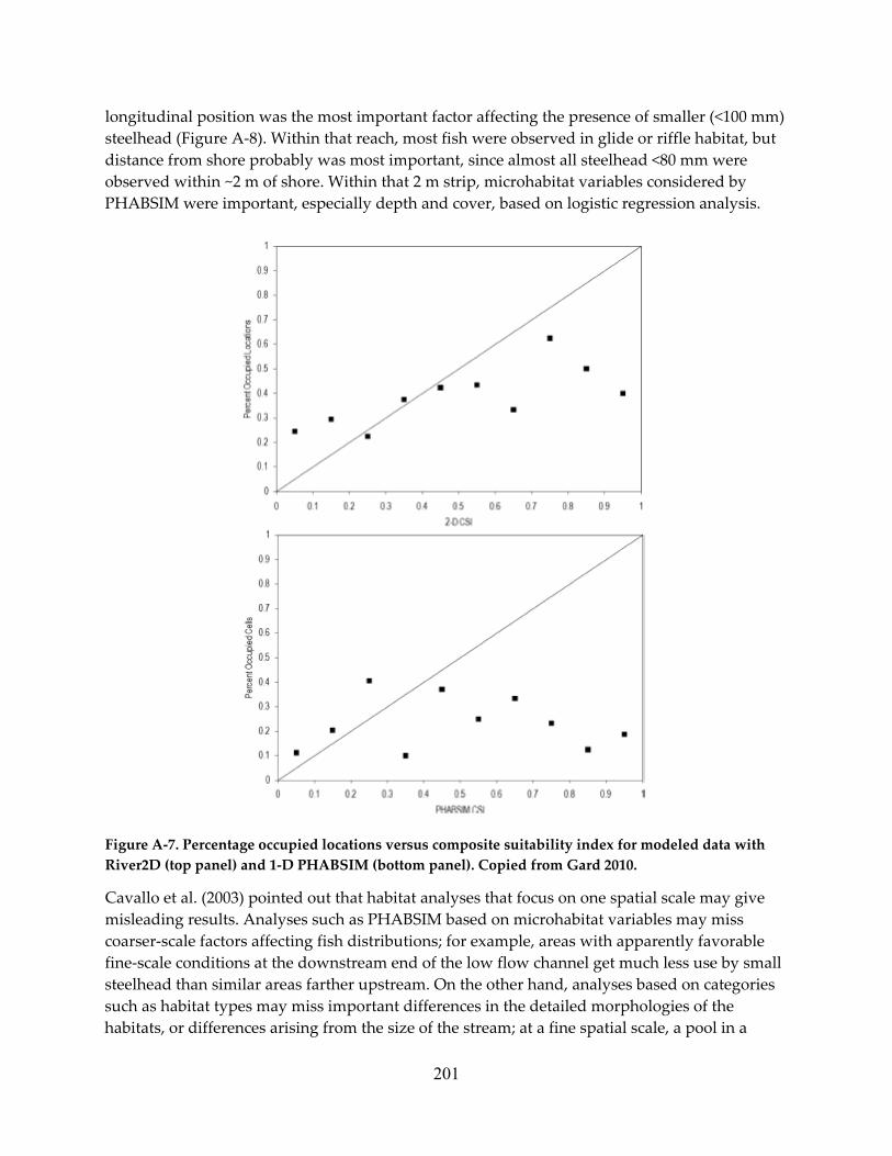
longitudinal position was the most important factor affecting the presence of smaller (<100 mm) steelhead (Figure A‐8). Within that reach, most fish were observed in glide or riffle habitat, but distance from shore probably was most important, since almost all steelhead <80 mm were observed within ~2 m of shore. Within that 2 m strip, microhabitat variables considered by PHABSIM were important, especially depth and cover, based on logistic regression analysis.

Figure A‐7. Percentage occupied locations versus composite suitability index for modeled data with River2D (top panel) and 1‐D PHABSIM (bottom panel). Copied from Gard 2010.

Cavallo et al. (2003) pointed out that habitat analyses that focus on one spatial scale may give misleading results. Analyses such as PHABSIM based on microhabitat variables may miss coarser‐scale factors affecting fish distributions; for example, areas with apparently favorable fine‐scale conditions at the downstream end of the low flow channel get much less use by small steelhead than similar areas farther upstream. On the other hand, analyses based on categories such as habitat types may miss important differences in the detailed morphologies of the habitats, or differences arising from the size of the stream; at a fine spatial scale, a pool in a

201

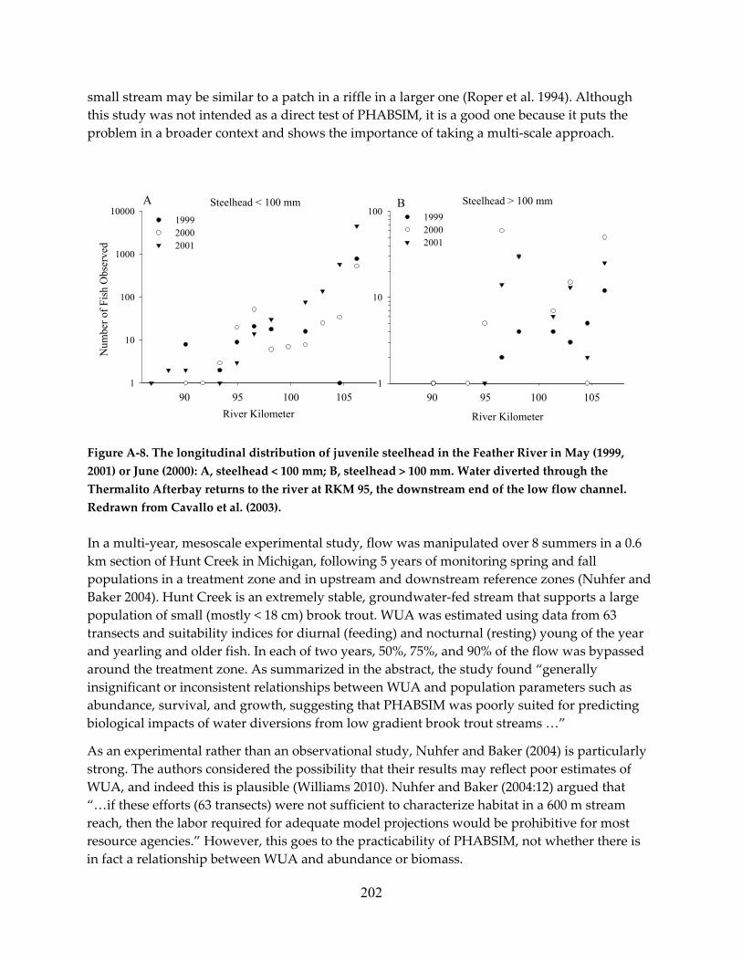
small stream may be similar to a patch in a riffle in a larger one (Roper et al. 1994). Although this study was not intended as a direct test of PHABSIM, it is a good one because it puts the problem in a broader context and shows the importance of taking a multi‐scale approach.

Steelhead < 100 mm

River Kilometer90 95 100 105

Num

ber o

f Fis

h O

bser

ved

1

10

100

1000

100001999 2000 2001

Steelhead > 100 mm

River Kilometer

1

10

100

90 95 100 105

A B1999 2000 2001

Figure A‐8. The longitudinal distribution of juvenile steelhead in the Feather River in May (1999, 2001) or June (2000): A, steelhead < 100 mm; B, steelhead > 100 mm. Water diverted through the Thermalito Afterbay returns to the river at RKM 95, the downstream end of the low flow channel. Redrawn from Cavallo et al. (2003).

In a multi‐year, mesoscale experimental study, flow was manipulated over 8 summers in a 0.6 km section of Hunt Creek in Michigan, following 5 years of monitoring spring and fall populations in a treatment zone and in upstream and downstream reference zones (Nuhfer and Baker 2004). Hunt Creek is an extremely stable, groundwater‐fed stream that supports a large population of small (mostly < 18 cm) brook trout. WUA was estimated using data from 63 transects and suitability indices for diurnal (feeding) and nocturnal (resting) young of the year and yearling and older fish. In each of two years, 50%, 75%, and 90% of the flow was bypassed around the treatment zone. As summarized in the abstract, the study found “generally insignificant or inconsistent relationships between WUA and population parameters such as abundance, survival, and growth, suggesting that PHABSIM was poorly suited for predicting biological impacts of water diversions from low gradient brook trout streams …”

As an experimental rather than an observational study, Nuhfer and Baker (2004) is particularly strong. The authors considered the possibility that their results may reflect poor estimates of WUA, and indeed this is plausible (Williams 2010). Nuhfer and Baker (2004:12) argued that “…if these efforts (63 transects) were not sufficient to characterize habitat in a 600 m stream reach, then the labor required for adequate model projections would be prohibitive for most resource agencies.” However, this goes to the practicability of PHABSIM, not whether there is in fact a relationship between WUA and abundance or biomass.

202

Of course, it can be argued that PHABSIM or other NHMs models habitat, not fish abundance or biomass, and there are many reasons why abundance or biomass might not be related to habitat in particular cases. However, as noted by Conder and Annear (1987:339), “Use of PHABSIM relies on the assumption that a positive linear relationship exists between WUA and physical habitat, with the implied assumption that a relationship exists between physical habitat and standing crop.” This assumption should be properly tested, with attention to good statistical practice; Burnham and Anderson (1998), Hilborn and Mangel (1997), Manley et al. (2002), and Johnson and Omland (2004) provide useful guidance. In any event, the results of PHABSIM studies should be reported with confidence intervals, as called for Castleberry et al. (1996). Model results of unknown reliability should not be relied upon.

References Ahmadi‐Nedushan, B., A. St‐Hilaire, M. Bérubé, E. Robichaud, N. Thiémonge, and B. Bobée.


Armour C. L. and J. G. Taylor. 1991. Evaluation of the instream flow incremental methodology by U.S. Fish and Wildlife Service field users. Fisheries 16:36‐43.

Annear, T., I. Chisholm, H. Beecher, A. Locke, P. Aarrestad, C. Coomer, C. Estes, J. Hunt, R. Jacobson, G. Jobsis, J. Kauffman, J. Marshall, K. Mayes, G. Smith, R. Wentworth, and C. Stalnaker. 2004. Instream flows for riverine resource stewardship. Instream Flow Council. Cheyenne, WY.

Behnke, R. J. 1986. Critique of instream flow methodologies. Unpublished manuscript. Booker D. J. and M. C. Acreman. 2007. Generalisation of physical habitat–discharge

relationships. Hydrology and Earth System Sciences 11:141–157. Bourgeois, G., R. A. C. Cunjak, and N. El‐Jabi. 1996. A spatial and temporal evaluation of

PHABSIM in relation to measured density of juvenile Atlantic salmon in a small stream. North American Journal of Fisheries Management 16:154‐166.

Bovee, K.D. and J .R. Zuboy. 1988. Proceedings of a Workshop on the Development and Evaluation of Habitat Suitability Criteria. U.S. Fish and Wildlife Service BioI. Rep. 88 (11): 407 pp.


Cade, B. S. and J. W. Terrell. 1997. Comment: cautions on forcing regression equations through the origin. North American Journal of Fisheries Management 17:225‐227.

Castleberry, D. T., J. J. Cech, D. C. Erman, D. Hankin, M. Healey, G. M. Kondolf, M. Mangel, M. Mohr, P. B. Moyle, J. Nielsen, T. P. Speed, and J. G. Williams. 1996. Uncertainty and instream flow standards. Fisheries 21:20‐21.

Cavallo, B., R. Kurth, J. Kindoff, A. Seesholtz, and M. Perrone. 2003. Distribution and habitat use of steelhead and other fishes in the lower Feather River, 1999‐2001. California Department of Water Resource, Sacramento, CA.

203

Conder, A. L. and T. C. Annear. 1987. Test of weighted usable area estimates derived from a PHABSIM model for instream flow studies on trout streams. North American Journal of Fisheries Management 7: 339‐350.

Freedman, D. A. 1983. A note on screening regression equations. The American Statistician 37:152‐155.

Freedman, D. A. 1999. Ecological inference and the ecological fallacy. Department of Statistics, University of California,. Technical Report No. 549. Berkeley, CA.

Fretwell, S. D. 1972. Populations in a seasonal environment. Princeton University Press. Princeton, NJ.

Gallagher, S. P. and M. F. Gard. 1999. Relationship between Chinook salmon (Oncorhynchus tshawytscha) redd densities and PHABSIM‐predicted habitat in the Merced and Lower American rivers, California. Canadian Journal of Fisheries and Aquatic Sciences 56:570‐577.

Gard, M. F. 2009. Demonstration flow assessment and 2‐D modeling: perspectives based on instream flow studies and evaluation of restoration projects. Fisheries 34:320‐329.

Gard, M. F. 2010. Response to Williams (2009) on Gard (2009): comparison of spawning habitat predictions of PHABSIM and River2D models. International Journal of River Basin Management 8:121‐125.

Gore, J. A., D. J. Crawford, and D. S. Addison. 1998. An analysis of artificial riffles and enhancement of benthic community diversity by physical habitat simulation (PHABSIM) and direct observation. Regulated Rivers: Research and Management 14:69‐77.


Guisan A. and N. E. Zimmermann. 2000. Predictive habitat distribution models in ecology. Ecological Modelling 135:147‐186.

Healey, M. C. 1991. Life history of chinook salmon (Oncorhynchus tshawytscha). In: Groot, C, Margolis, L, editors. Pacific salmon life histories. p. 311‐394.

Heggenes, J. 2002. Flexible summer habitat selection by wild, allopatric brown trout in lotic environments. Transactions of the American Fisheries Society 131:287‐298.

Hilborn R and M. Mangel. 1997. The ecological detective: confronting models with data. Monographs in Population Biology. Princeton University Press. Princeton, NJ.

Holm, C. F., J. D. Armstran, and D. J. Gilvear. 2001. Investigating a major assumption of predictive instream habitat models: is water velocity preference of juvenile Atlantic salmon independent of discharge. Journal of Fish Biology 59:1653‐1666.

Huntingford, F. A., N. B. Metcalf, and J. E. Thorpe. 1988. Choice of feeding station in Atlantic salmon, Salmo salar parr: effects of predation risk, season and life history strategy. Journal of Fish Biology 33:917‐924.

Johnson, J. B. and K. S. Omland. 2004. Model selection in ecology and evolution. Trends in Ecology and Evolution 19:101‐108.

Jowett I. G. 1992. Models of abundance of large brown trout in New Zealand Rivers. North American Journal of Fisheries Management 12:417‐432.

204

Jowett, I. G. 2000. Expert evidence presented on the resource consent application of Genesis Power Ltd. to operate the Tongariro Power Development. Hearing held in Taupo, New Zealand, December 2000. Genesis Power Ltd., Tokaanu, NZ.

Jowett I. G. and A. J. H Davey. 2007. A comparison of composite habitat suitability indices and generalized additive models of invertebrate abundance and fish presence‐habitat availability. Transactions of the American Fisheries Society 136:428–444.

Kemp, P. S., D. J. Gilvear, and J. D. Armstrong. 2003. Do juvenile Atlantic salmon parr track local changes in water velocity. Rivers: Research and Applications 19:569‐575.

Lancaster, J. and B. J. Downes. 2010a. Linking the hydraulic world of individual organisms to ecological processes: putting ecology into ecohydraulics. River Research and Applications 26:385‐403.

Lancaster, J. and B. J. Downes. 2010b. Ecohyrdaulics needs to embrace ecology and sound science, and to avoid mathematical artefacts. River Research and Applications 26: 921–929.

Loar, J. M. 1985. Application of habitat evaluation models in southern Appalachian trout streams. Oak Ridge National Laboratory, Environmental Sciences Division, Publication 2823.


Nehring R. B. and R. M. Anderson. 1993. Determination of population‐limiting critical salmonid habitats in Colorado streams using the Physical Habitat Simulation System. Rivers 4:1‐19.

Nuhfer, A. J. and E. A. Baker. 2004. A long‐term field test of habitat change predicted by PHABSIM in relation to brook trout population dynamics during controlled flow reduction experiments. Fisheries Research Report 2068. Fisheries Division, Michigan Department of Natural Resources.

Oreskes, N. and K. Belitz. 2001. Philosophical issues in model assessment. Pages 23‐42 in Anderson M. G., and P. D. Bates, editors. Model validation: perspectives in hydrological science. John Wiley and Sons.

Orsborn, J. F. and C. H. E. Alolman. 1976. Editors. Proceedings of the symposium and specialty conference on instream flow needs, May 3‐6, 1976; Boise, Idaho. American Fisheries Society. Bethesda, MD.

Orth, D. J. and O. E Maughan. 1982. Evaluation of the Incremental Methodology for recommending instream flows for fishes. Transactions of the American Fisheries Society 111:413‐445.

Parasiewicz, P. 2001. MesoHABSIM: a concept for application of instream flow models in river restoration planning. Fisheries 26:6‐13.

Pert, E.J. and D. C. Erman. 1994. Habitat use by adult rainbow trout under moderate artificial fluctuations in flow. Transactions of the American Fisheries Society 123:913‐923.

Power, M. E., R. J. Stout, C. E. Cushing, P. P. Harper, F. R. Hauer, W. J. Matthews, P. B. Moyle, B. Statzner, and I. R. Wais de Badgen. 1988. Biotic and abiotic controls in river and stream communities. Journal of the North American Benthological Society 7:456‐479.

205

Railsback, S. F., H. B. Stauffer, and B. C. Harvey. 2003. What can habitat preference models tell us? Tests using a virtual trout population. Ecological Applications 13:1580‐1594.

Reiser D. W., T. A. Wesche, and C. Estes. 1989. Status of instream flow legislation and practices in North America. Fisheries 14:22‐29.

Roper, B. B., D. L. Scarnecchia, and T. J. La Marr. 1994. Summer distribution of and habitat use by Chinook salmon and steelhead with a major basin of the South Umpqua River, Oregon. Transactions of the American Fisheries Society 123:298‐308.

Vadas, R. L. and D. J. Orth. 2001. Formulation of habitat suitability models for stream fish guilds: do the standard methods work? Transactions of the American Fisheries Society 130:217‐235.

Van Horne B. 1982. Density as a misleading indicator of habitat quality. Journal of Wildlife Management 47:893‐901.

Vondracek B and D. R. Longanecker. 1993. Habitat selection by rainbow trout Oncorhynchus mykiss in a California stream: implications for the Instream Flow Incremental Methodology. Ecology of Freshwater Fish 2:137‐186.

Williams, J. G. 2001. Testing models used for instream flow assessment. Fisheries 26:19‐20. Williams, J. G. 2006. Central valley salmon: a perspective on Chinook and steelhead in the

Central Valley of California. San Francisco Estuary and Watershed Science Volume 4, Issue 3, Article 2. [Available online] URL: http://escholarship.org/uc/item/21v9x1t7

Williams, J. G. 2010c. Comment on Gard (2009): comparison of spawning habitat predictions of PHABSIM and River2D models. International Journal of River Basin Management 8:117‐119.

Zorn T. G. and P. W. Seelbach. 1995. The relation between habitat availability and the short‐term carrying capacity of a stream reach for smallmouth bass. North American Journal of Fisheries Management 15:773‐783.

206

http://escholarship.org/uc/item/21v9x1t7

Appendix B. Resource Selection Functions

The statistical aspects of detecting habitat or resource selection (or avoidance) are considered at length by Manly et al. (2002). With appropriate data, such as a census of used and unused patches of habitat and measured attributes of the patches, it is possible to define a resource selection probability function that gives the probability that a patch of habitat with given attribute values will be used, given that conditions, such as the population size at the time the census, stay the same. More commonly, as when use and attribute data are available only for samples of the patches, it is still possible to define a resource selection function that return a value proportional to the probability that a patch of habitat will be used. There is now a large literature on resource selection functions (Google Scholar lists over a thousand citations to Manly et al. 2002); these are mostly analyses of habitat use by birds and mammals, but a few concern fish.

A limitation of resource selection functions is that the probability that a given patch of habitat will be used must depend on factors such as size of the population of animals; that is, the function depends on the particular set of circumstances in which it is developed. As Manly et al. (2002) note, even for a given set of habitat patches, the probability of use may vary with the season, the time of day, the activities being pursued by the animals, etc. It may be reasonable to expect that a habitat selection function determined in one set of circumstances will be broadly applicable, but this is something that must be justified biologically; it does not come out of the statistics.

The typical habitat suitability criteria (HSC) used in PHABSIM are something like habitat selection functions. In fact, in the early literature, HSC were sometimes called “probability of use” curves (e.g., Bovee 1978, Shepard and Johnson 1985). It seems useful to think of resource selection functions as statistically defensible composite suitability criteria. The basic assumptions of resource selection functions are (Manly et al. 2002:43):

a. the distributions of the measured X variables for the available resource units and the resource selection probability function do not change during the study period;

b. the population of resource units available to the organisms has been correctly identified;

c. the subpopulations of used and unused resource units have been correctly identified;

d. the X variables which actually influence the probability of selection have been correctly identified and measured;

e. organisms have free and equal access to all available resource units; and

f. when studies involve the sampling of resource units, these units are sampled randomly and independently.

207

In practice, these assumptions are hard to meet in environmental flow studies. For example, territorial behavior by the fish under study may deny subordinate fish free and equal access to all available resource units, or variables other than those measured may have significant influence on habitat selection. The assumption that resource units are sampled randomly could be met, but seldom is (Williams 2010, Downes 2010). Nevertheless, relating the value of the suitability index to the probability of use gives the index a clear meaning, which other statistics such as composite suitability criteria lack. However, resource selection functions are abundance‐environment relations (AERs), as defined by Lancaster and Downes (2010), and have the limitations that they discuss.

Logistic regression is an attractive approach for developing AERs for use in NHMs, although others can be used as well. Many standard statistical programs will perform logistic regression and calculate standard errors for the coefficients, but as with other statistical procedures, the ease with which the programs can be used makes it is easy to go wrong. Consulting books such as Manly et al. (2002) regarding the assumptions of the method and the particulars of the intended application will help minimize this risk.

Since resource selection functions return a value that is proportional to the probability that a given patch of habitat will be used (given the assumptions), the spatial scale of the patch matters, since the probability that a large patch of habitat will be used may be very close to one. For larger patches, such as a salmon spawning riffle, it may be more appropriate to model the number of animals that use the patch, in which case Poisson regression could be used. This assumes that the log of the mean number of animals using the patch is a linear combination of the habitat variables. However, the cells or tiles in 2D models are often of a size such that logistic regression will be appropriate, especially for larger fish. For larger patches, other statistical approaches such as generalized linear models or generalized additive models may also be useful (Ahmadi‐Nedushan et al. 2006).

For an example of a resource selection function applied to fish, For example, Knapp and Preisler (1999) used logistic regression in a study of spawning site selection by golden trout, and selected depth, depth squared, velocity, velocity squared, substrate size, substrate size squared, and the natural log of stream width as explanatory habitat variables from a larger set, based on the Akaike information criterion. Logistic regression has zero and one as limiting values for the dependent variable θ, and

= 1 / (1 + e‐λ)

λ = exp(β0 + β1X1 + β2X2 + ... + βnXn)

where λ is a function of the habitat variables Xi and the fitted coefficients βi.

For spawning site selection by Chinook in the Feather River, where the density of spawning increases upstream, DWR (2010) proposes to test a set of models using variables that include location variables, such as river mile or channel feature (e.g., riffle crest), the traditional microhabitat variables, hyporheic variables, and indicator variables such as whether a riffle has been treated, or example:

208

λ = βo + β1RM + β2Perm

λ = βo + β1RM + β2Perm + β3Vel + β4Vel2

λ = βo + β1Depth + β2Depth2 + β3Vel + β4Vel2 + β5D50 + β6D502)

λ = βo + β1RM + β2Depth + β3Depth2 + β4Vel + β5Vel2 + β6D50 + β7D502 + β8Treat)

where RM is river mile, Perm is some measure of permeability, Vel is velocity, D50 is the median gravel size, and Treat is an indicator variable (Treat = 1 if the riffle has been treated, else 0). Here, the third equation is similar to the standard PHABSIM approach.

In general, adding more variables and associated parameters to a model will give a better fit to the data, so this should be taken into account when assessing how well the model fits the data, and whether particular variables should be included. Statistical criteria such as the Akaike Information Criterion (AIC; Burnham and Anderson 1999), the Bayesian Information Criterion (BIC; Schwartz 1978), or the Deviance Information Criterion (DIC; Spiegelhalter et al. 2002) can be used for deciding which variables to include, but the selection of variables should also make biological sense.

The models described so far can be fit using either traditional or Bayesian methods. Bayesian methods use the data to update “prior” probability distributions for the parameters of the model; the updated or “posterior” probability distribution is proportional to the “likelihood,” of the model, times the prior probability distribution. Stated differently, the probability of the model given the data is proportional to the probability of the data given the model (the likelihood) times the prior probability of the model. With this approach, other sources of information besides the data at hand can be incorporated into the estimation of the parameters, which may be a major advantage. For example, data from spawning studies in other streams could be used to specify the prior probability distributions. In other cases, however, traditional methods give essentially the same result, so the need to specify prior distributions may simply be a complication.

As another example of a resource selection function applied to fish, although it was not identified as such, Guay et al. (2000) used logistic regression to developed a Habitat Probabilistic Index (HPI) for juvenile Atlantic salmon in the Sainte‐Marguerite River in Quebec, using depth, velocity, substrate and depth squared as variables. Traditional suitability criteria for depth, velocity and substrate have the virtue of being transparent. Typically the criteria are plotted, so that their biological plausibility can be assessed, and if the criteria are combined by simple multiplication is reasonably easy to assess the effect of each on combined score for the habitat cell. It is more complicated, but still worthwhile, to do the same for logistic regression, as we show by an exploration of the HPI. As a first step to understanding the model and assessing its biological plausibility, it is useful to plot the basic equation (Figure B‐1). HPI increases rapidly with λ from about ‐2 to +2, and more slowly outside that region. Increases in the absolute value of λ beyond about 3 make little difference.

209

Lambda

-4 -2 0 2 4

HP

I

0.0

0.2

0.4

0.6

0.8

1.0

Figure B‐1. Logistic regression model for the HPI (or

As candidate variables, Guay et al. (2000) considered:

λ = β0 + β1S + β2V + β3D + β4 S2 + β5V2 + β6D2 + ...

Depth (m)

0.0 0.2 0.4 0.6 0.8 1.0 1.2 1.4

pp

q

Dep

th c

ontri

butio

n to

lam

bda

0

1

2

3

where S, V and D are median substrate size (D50), water velocity, and water depth. The parameters β n were estimated from data, using stepwise backward regression, and the parameters and values that gave the simplest statistically significant model were selected, resulting in β0 = ‐3.067, β1 = 0.093, β2 = 2.86, β 3 = 8.461, and β6 = ‐6.203. According, λ increases linearly with sediment size and water velocity, (β 1 and β 2), but is quadratic in depth (β 3 and β 6).

Figure B‐2. Contribution of depth to λ in the model for the HPI

210

Thus, pool habitat with a sandy substrate would have a very low HPI, and HPI would be maximal in habitat with the highest water velocity, coarsest substrate, and a depth of 0.68 m. For the range of the data, with maximum water velocity of 1.2 m/s and D50 of 16 cm, λ will peak at 4.71, with contributions from depth of 2.86, substrate of 1.49, and velocity of 3.43. The contributions of depth, velocity, and substrate to λ are plotted in Figure B‐2 and B‐3.

Despite the linear relation in the model, the juvenile salmon observed by Guay et al. (2000) preferred cells with smaller sediment (their Figure 3a), with preference peaking for substrate with a D50 of 3 or 4 cm, which seems inconsistent with the parameterization of the model.

Water Velocity (ms-1)

0.0 0.2 0.4 0.6 0.8 1.0 1.2

Con

tribu

tion

to L

ambd

a

0

1

2

3

Con

tribu

tion

to L

ambd

a

Substrate D50 (cm)

0 3 6 9 12 15 180

1

2

3

Figure B‐3. Contribution of water velocity (top panel) and substrate D50 (bottom panel) to λ in the model for the HPI

With the substrate D50 of 4 cm (S = 4), curves of HPI over depth are humped, because HPI is quadratic in depth, and as velocity increases the hump becomes higher and broader (Figure B‐4). For higher values of S, the curves are higher and even broader, especially for low water

211

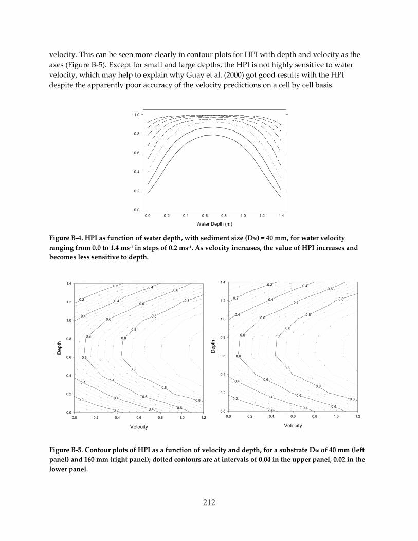
velocity. This can be seen more clearly in contour plots for HPI with depth and velocity as the axes (Figure B‐5). Except for small and large depths, the HPI is not highly sensitive to water velocity, which may help to explain why Guay et al. (2000) got good results with the HPI despite the apparently poor accuracy of the velocity predictions on a cell by cell basis.

Water Depth (m)

0.0 0.2 0.4 0.6 0.8 1.0 1.2 1.40.0

0.2

0.4

0.6

0.8

1.0

Figure B‐4. HPI as function of water depth, with sediment size (D50) = 40 mm, for water velocity ranging from 0.0 to 1.4 ms‐1 in steps of 0.2 ms‐1. As velocity increases, the value of HPI increases and becomes less sensitive to depth.

0.0

0.2

0.4

0.6

0.8

1.0

1.2

1.4

0.0

0.2

0.4

0.6

0.8

1.0

1.2

1.4

Velocity

0.0 0.2 0.4 0.6 0.8 1.0 1.2

Dep

th

0.8

0.8

0.8

0.8

0.8

0.8

0.6

0.6

0.6

0.6

0.6

0.6

0.6

0.4

0.4

0.4

0.4

0.4

0.4

0.8

0.2

0.2

0.2

0.2

0.6

0.8

0.8

0.8

0.8

0.8

0.8

0.6

0.6

0.6

0.6

0.6

0.6

0.6

0.4

0.4

0.4

0.4

0.4

0.4

0.8

0.2

0.2

0.2

0.2

0.6

Velocity

Dep

th

0.0 0.2 0.4 0.6 0.8 1.0 1.2

Figure B‐5. Contour plots of HPI as a function of velocity and depth, for a substrate D50 of 40 mm (left panel) and 160 mm (right panel); dotted contours are at intervals of 0.04 in the upper panel, 0.02 in the lower panel.

212

213

It could be informative to plot calibration data on similar axes, which might identify values of the physical variables where the index would be more or less reliable. For example, based on Figure 3 in Guay et al. (2000), it seems that there are few calibration data for large values of S, so that predictions of the HPI in that region of parameter space would be less reliable. It might be useful to plot deviations from model predictions in a similar way. The point is that simply fitting a resource selection function to data in not really enough; it should be examined carefully before it is used.

References Ahmadi‐Nedushan, B., A. St‐Hilaire, M. Bérubé, E. Robichaud, N. Thiémonge, and B. Bobée.


Bovee, K. D. 1978. Probability‐of‐use criteria for the Family Salmonidae. U. S. Fish and Wildlife Service, Cooperative Instream Flow Service Group. Fort Collins, CO.


Department of Water Resources (DWR). 2010. Draft Feather River gravel supplementation program: Settlement Agreement Section A102. Oroville Facilities, FERC Project No. 2100. California Department of Water Resources.

Downes, B. J. 2010. Back to the future: little‐used tools and principles of scientific inference can help disentangle effects of multiple stressors on freshwater ecosystems. Freshwater Biology 55(Suppl. 1):60‐79.


Knapp, R. A. and H. K. Preisler. 1999. Is it possible to predict habitat use by spawning salmonids: a test using golden trout (Oncorhynchus mykiss aguabonita). Canadian Journal of Fisheries and Aquatic Sciences 56:1576‐1584.

Lancaster, J. and B. J. Downes. 2010. Linking the hydraulic world of individual organisms to ecological processes: putting ecology into ecohydraulics. River Research and Applications 26:385‐403.


Spiegelhalter, D. J., N. G. Best, B. P. Carlin, and A. van der Linde. 2002. Bayesian measures of model complexity and fit. Journal of the Royal Statistical Society B 64:583‐639.

Williams, J. G. 2010. Lost in space, the sequel: spatial sampling issues with 1‐D PHABSIM. River Research and Applications 26:341‐352.

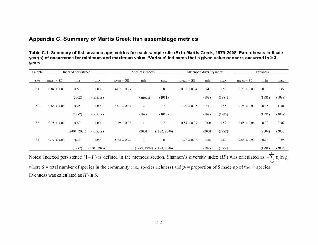
Appendix C. Summary of Martis Creek fish assemblage metrics

Table C.1. Summary of fish assemblage metrics for each sample site (S) in Martis Creek, 1979-2008. Parentheses indicate year(s) of occurrence for minimum and maximum value. ‘Various’ indicates that a given value or score occurred in ≥ 3 years.

Sample

site mean ± SE min max mean ± SE min max mean ± SE min max mean ± SE min max

S1 0.84 ± 0.03 0.50 1.00 4.07 ± 0.23 3 8 0.98 ± 0.04 0.41 1.50 0.73 ± 0.03 0.30 0.95

(2002) (various) (various) (1981) (1988) (1981) (1988) (1998)

S2 0.86 ± 0.03 0.25 1.00 4.07 ± 0.25 2 7 1.00 ± 0.05 0.31 1.58 0.75 ± 0.03 0.45 1.00

(1987) (various) (1988) (1980) (1988) (1993) (1988) (2008)

S3 0.75 ± 0.04 0.40 1.00 3.79 ± 0.27 1 7 0.84 ± 0.07 0.00 1.52 0.65 ± 0.04 0.00 0.96

(2004, 2005) (various) (2004) (1982, 2006) (2004) (1982) (2004) (2000)

S4 0.77 ± 0.03 0.33 1.00 5.62 ± 0.23 3 8 1.08 ± 0.06 0.28 1.60 0.64 ± 0.03 0.26 0.89

(1987) (2002, 2008) (1987, 1988) (1984, 2006) (1988) (2004) (1988) (2004)

Indexed persistence Species richness EvennessShannon's diversity index

Notes: Indexed persistence (1 T− ) is defined in the methods section. Shannon’s diversity index (H’) was calculated as 1

ln S

i iS

p p=

−∑

where S = total number of species in the community (i.e., species richness) and pi = proportion of S made up of the ith species.

Evenness was calculated as H’/ln S.

214

Appendix D. Bayesian Networks for Improving Environmental Flow Assessments in FERC Licensing Processes in California

Phase II Concept Proposal Submitted to the Instream Flow Program, California Energy Commission

PI: Dr. Peter Moyle, Center for Watershed Sciences, University of California, Davis, CA 95616 [email protected]

Co‐PIs: Dr. Jeffrey Mount (UC Davis), Dr. G. Mathias Kondolf (UC Berkeley)

Summary:

Bayesian Networks have emerged as a highly useful tool for synthesizing and evaluating information from diverse sources in environmental assessments, especially in the context of stakeholder processes (Marcot et al. 2001, 2006, Stevenson 2008, Hart and Polino 2009). In our currently funded work, we have been attracted to Bayesian Networks (BNs) as a useful tool for environmental flow assessment that seems well suited for FERC licensing processes. For Phase two of our project, we propose to develop a set of template Bayesian Networks, developed particularly for Sierra Nevada/Southern Cascade Mountain streams. These could be used in the development of FERC‐related study plans, in synthesizing information from site‐specific and literature studies, in assessing the probable consequences of particular flow regimes, and in designing post‐license monitoring programs. For this project, we propose to:

1. Develop template BNs that could be adapted for particular Sierran/Cascadian streams or watersheds, dealing with brown trout, rainbow trout, yellow‐legged frogs, sediment transport, and riparian vegetation, as well as other species depending streams selected.

2. Fully develop selected BNs to one larger and one smaller stream for which considerable data exist and to which conventional methods such as PHABSIM have been applied.

Introduction:

A final deliverable in our project “Improving Environmental Flow Methods used in California FERC Licensing” is to recommend two streams (“test beds”) that could be used for comparative applications of different Environmental Flows Assessments (EFAs) and to develop a proposal for making those comparisons. However, in our ongoing work, we have been attracted to Bayesian Networks (BNs) as a useful tool for synthesizing and evaluating information in environmental flow assessment. We think that developing BNs for EFAs will accomplish the same goal of improving EFAs as in our original proposal but potentially have a more far‐reaching impact on EFAs, making studies from different streams more comparable and making

215


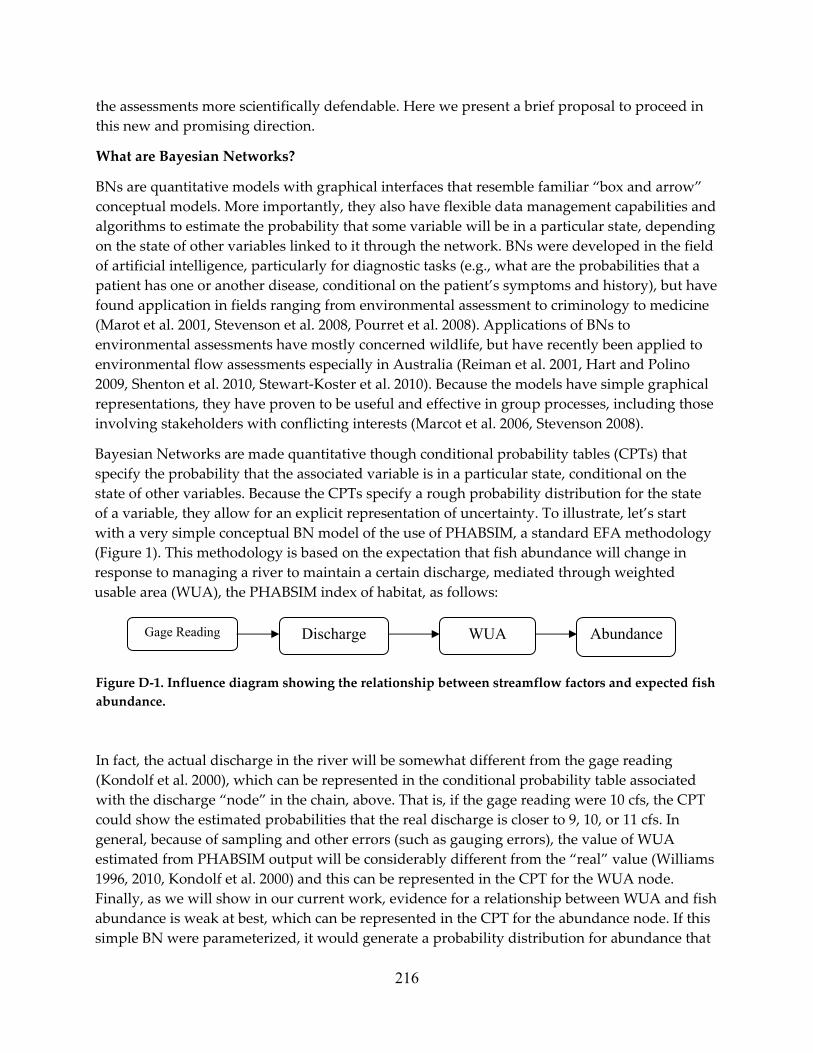
the assessments more scientifically defendable. Here we present a brief proposal to proceed in this new and promising direction.

What are Bayesian Networks?

BNs are quantitative models with graphical interfaces that resemble familiar “box and arrow” conceptual models. More importantly, they also have flexible data management capabilities and algorithms to estimate the probability that some variable will be in a particular state, depending on the state of other variables linked to it through the network. BNs were developed in the field of artificial intelligence, particularly for diagnostic tasks (e.g., what are the probabilities that a patient has one or another disease, conditional on the patient’s symptoms and history), but have found application in fields ranging from environmental assessment to criminology to medicine (Marot et al. 2001, Stevenson et al. 2008, Pourret et al. 2008). Applications of BNs to environmental assessments have mostly concerned wildlife, but have recently been applied to environmental flow assessments especially in Australia (Reiman et al. 2001, Hart and Polino 2009, Shenton et al. 2010, Stewart‐Koster et al. 2010). Because the models have simple graphical representations, they have proven to be useful and effective in group processes, including those involving stakeholders with conflicting interests (Marcot et al. 2006, Stevenson 2008).

Bayesian Networks are made quantitative though conditional probability tables (CPTs) that specify the probability that the associated variable is in a particular state, conditional on the state of other variables. Because the CPTs specify a rough probability distribution for the state of a variable, they allow for an explicit representation of uncertainty. To illustrate, let’s start with a very simple conceptual BN model of the use of PHABSIM, a standard EFA methodology (Figure 1). This methodology is based on the expectation that fish abundance will change in response to managing a river to maintain a certain discharge, mediated through weighted usable area (WUA), the PHABSIM index of habitat, as follows:

Discharge WUA Abundance Gage Reading

Figure D‐1. Influence diagram showing the relationship between streamflow factors and expected fish abundance.

In fact, the actual discharge in the river will be somewhat different from the gage reading (Kondolf et al. 2000), which can be represented in the conditional probability table associated with the discharge “node” in the chain, above. That is, if the gage reading were 10 cfs, the CPT could show the estimated probabilities that the real discharge is closer to 9, 10, or 11 cfs. In general, because of sampling and other errors (such as gauging errors), the value of WUA estimated from PHABSIM output will be considerably different from the “real” value (Williams 1996, 2010, Kondolf et al. 2000) and this can be represented in the CPT for the WUA node. Finally, as we will show in our current work, evidence for a relationship between WUA and fish abundance is weak at best, which can be represented in the CPT for the abundance node. If this simple BN were parameterized, it would generate a probability distribution for abundance that

216

would be expected from a given flow release, given the probability values in the CPTs. This would provide a more realistic picture of the likely outcome than the single values that tend to come from more standard analyses.

The probability values in the CPTs can be estimated directly from data, from output of other models, or from expert opinion, which makes BNs useful for integrating different kinds of information from various sources. For EFA, BNs could integrate the results of more traditional approaches with results from new approaches such as the dynamic energy budget models or response length models currently under development with IFP funding.

Applying BNs to EFAs in California

A major recommendation of our current project is that a set of “off the shelf” or template BNs be developed for Sierran streams, that could be used in FERC licensing processes. These could include BNs at several spatial scales (stream reach to basin) for trout and other fishes, yellow‐legged frogs, and riparian vegetation. BNs could even be developed for white‐water recreation. The networks can be nested; for example, Marcot et al. (2001) developed BNs for the effects of forest management on Townsend’s big‐eared bats at the scales of sites, sub‐watersheds, and basins, with outputs from the finer spatial scales feeding into the BNs at the next scale.

In our current work, we are developing BNs for fish abundance in Martis Creek, because the BNs can be parameterized from actual data, using Netica© software. An example is presented as Figure 2. In BNs designed for FERC processes, we expect that many CPTs would have to be filled out by expert opinion, or by stakeholder consensus, backed by studies such as our Martis Creek analysis. Filling in the CPTs is reported to be a useful process for eliciting and resolving differences of opinion among the stakeholders, but if the stakeholders cannot agree, then different versions of the BNs can be maintained so that the negotiations can continue (Hart and Polino 2009), and when the BNs are completed and exercised, the importance of the disagreements for the outcomes of actual interest can be quantified.

As we envision it, stakeholders would use the template BNs as a starting point for discussing and agreeing upon conceptual models for their particular streams and for making modifications in the BNs based on local knowledge. Similarly, they would use the CPTs for guidance regarding information needed from stream‐specific studies that would be conducted as part of the process. They would need help from consultants familiar with BNs, but given the growing popularity of the method, these should be available in the near future.

Budget:

Personnel necessary for the two‐year project include a full‐time post‐doc familiar with the technical details and mathematical underpinnings of BNs, and a part‐time senior scientist familiar with environmental flow assessment as well as the generalities of BNs, to provide guidance (Detailed budget omitted).

217

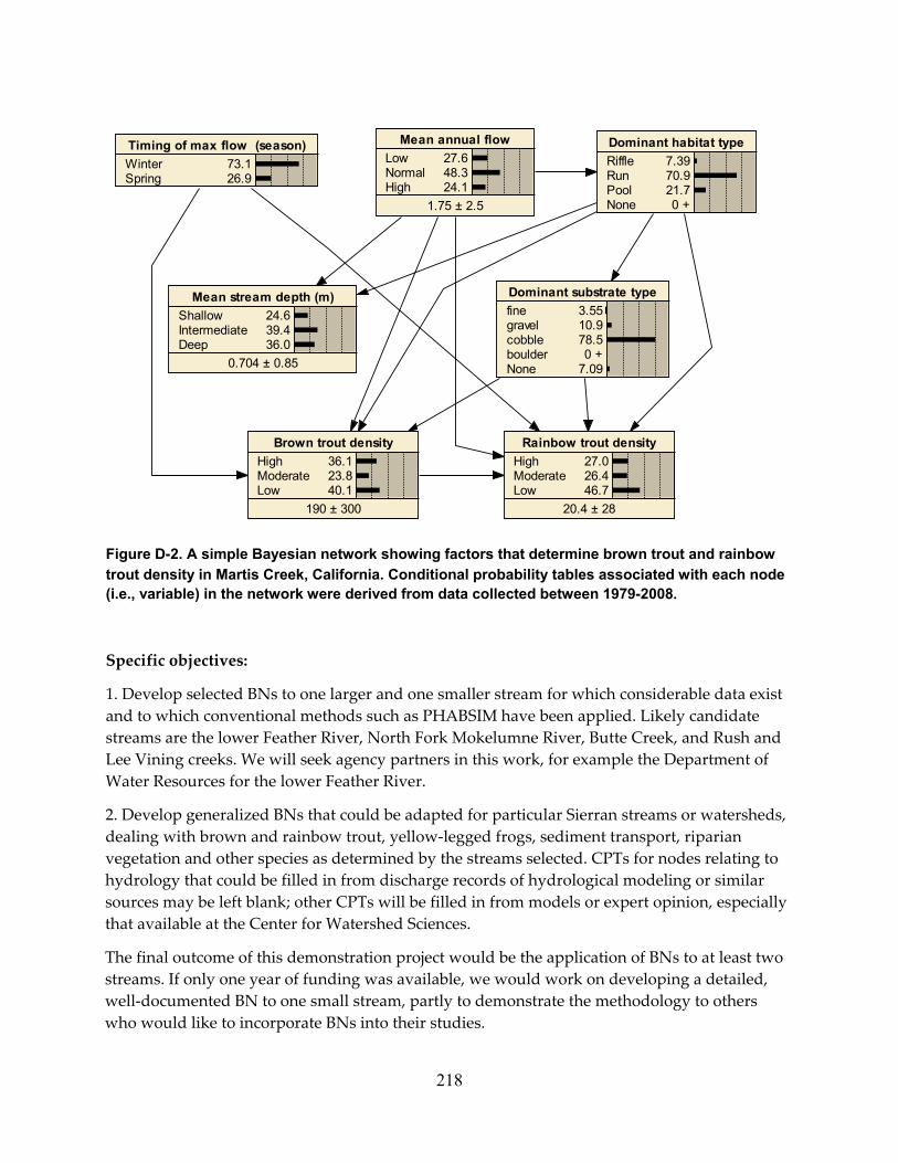
Rainbow trout densityHighModerateLow

27.026.446.7

20.4 ± 28

Mean annual flowLowNormalHigh

27.648.324.1

1.75 ± 2.5

Mean stream depth (m)ShallowIntermediateDeep

24.639.436.0

0.704 ± 0.85

Brown trout densityHighModerateLow

36.123.840.1

190 ± 300

Timing of max flow (season)WinterSpring

73.126.9

Dominant habitat typeRiffleRunPoolNone

7.3970.921.7 0 +

Dominant substrate typefinegravelcobbleboulderNone

3.5510.978.5 0 +7.09

Figure D-2. A simple Bayesian network showing factors that determine brown trout and rainbow trout density in Martis Creek, California. Conditional probability tables associated with each node (i.e., variable) in the network were derived from data collected between 1979-2008.

Specific objectives:

1. Develop selected BNs to one larger and one smaller stream for which considerable data exist and to which conventional methods such as PHABSIM have been applied. Likely candidate streams are the lower Feather River, North Fork Mokelumne River, Butte Creek, and Rush and Lee Vining creeks. We will seek agency partners in this work, for example the Department of Water Resources for the lower Feather River.

2. Develop generalized BNs that could be adapted for particular Sierran streams or watersheds, dealing with brown and rainbow trout, yellow‐legged frogs, sediment transport, riparian vegetation and other species as determined by the streams selected. CPTs for nodes relating to hydrology that could be filled in from discharge records of hydrological modeling or similar sources may be left blank; other CPTs will be filled in from models or expert opinion, especially that available at the Center for Watershed Sciences.

The final outcome of this demonstration project would be the application of BNs to at least two streams. If only one year of funding was available, we would work on developing a detailed, well‐documented BN to one small stream, partly to demonstrate the methodology to others who would like to incorporate BNs into their studies.

218

219

If we are successful (high probability) in this endeavor, we think FERC processes using EFAs could be greatly improved. At the very least, application of BNs could demonstrate that there is greater uncertainty in the outcomes of EFAs, especially for the standard methods such as PHABSIM, than is generally acknowledged. BNs can then provide a means to improve decision making in the face of uncertainty.

References:

Hart, B. T. and Polino, A. 2009. Bayesian modeling for risk‐based environmental water allocation. Waterlines Report. Canberra, Australia: National Water Commission.

Kondolf, G. M., Larsen E. W., and Williams, J. G. 2000. Measuring and modeling the hydraulic environment for assessing instream flows. North American Journal of Fisheries Management 20:1016‐1028.

Marcot, B. G., Holthausen, R. S., Raphael, M. G., Rowland, M. M., and Wisdom, M. J. 2001. Using Bayesian belief networks to evaluate fish and wildlife population viability under land management alternatives from an environmental impact statement. Forest Ecology and Management 153:29‐42.

Marcot, B. G., Stevenson, J. D., Sutherland, G. D., and McCann, R. K. 2006. Guidelines for developing and updating Bayesian belief networks applied to ecological modeling and conservation. Canadian Journal of Forest Research 36:3063‐3074.

Pourret, O., Naim, P., and Marcot, B. 2008. Bayesian networks: a practical guide to applications. John Wiley and Sons, Hoboken, NJ.

Reiman, B., Peterson J. T., Clayton, J., Howell, P., Thurow, R., Thompson, W., and Lee, D. 2001. Evaluation of potential effects of federal land management alternatives on trends of salmonids and their habitats in the interior Columbia basin. Forest Ecology and Management. 153:43‐62.

Shelton, W., Hart, B. T., and Chan, T. 2010. Bayesian network models for environmental flow decision‐making: I. Latrobe River Australia. River Research and Applications. (online, DOI:10.1002/rra.1348)

Stevenson, J. D. Conservation of marbled murrelets in British Columbia. 2008. Pourret, O., Naim, P., and Marcot, B., Editors. Bayesian Networks: a practical guide to applications. Hoboken, NJ: John Wiley and Sons, pp. 127‐148.

Stewart‐Koster, B., Bunn, S. E., MacKay, S. J., Poff, N. L., Naiman, R. J., and Lake, P. S. 2010. The use of Bayesian networks to guide investments in flow and catchment restoration for impaired river ecosystems. Freshwater Biology 55:243‐260.

Williams, J. G. 1996. Lost in space: minimum confidence intervals for idealized PHABSIM studies. 1996. Transactions of the American Fisheries Society 125:458‐465.

Williams, J. G. 2010. Lost in space, the sequel: spatial sampling issues with 1‐D PHABSIM. River Research and Applications 26:341‐352.

Governor IMPROVING ENVIRONMENTAL FLOW … · edmund g. brown, jr. governor. improving environmental...

Documents

Transcript of Governor IMPROVING ENVIRONMENTAL FLOW … · edmund g. brown, jr. governor. improving environmental...